


Languages
Pages
Legal

Eco-hydrological modeling in a mountain laboratory: the LTSER site Matsch/Mazia
Bertoldi G., Cordano E., Brenner J., Notarnicola. C., Niedrist G., Tappeiner U.
Workshop on coupled hydrological modeling, 23-‐24 September 2015, University of Padova, Italy.
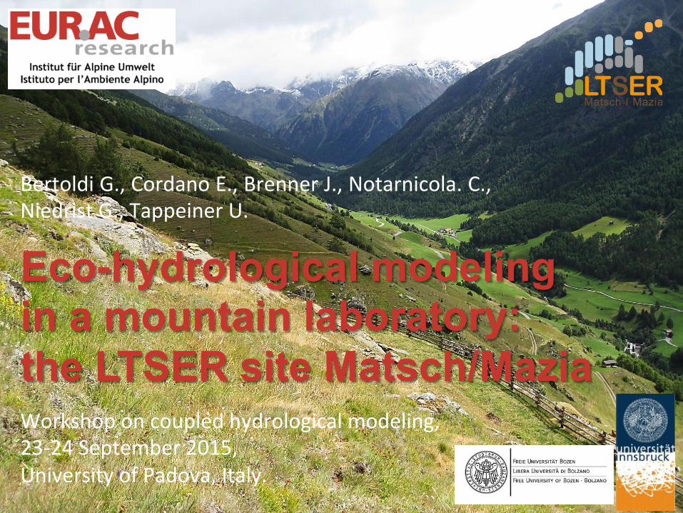
Outline Overview of the research area and of the collected data Modelling approach: the GEOtop 2 -‐ DV model.
Applica=ons : 1. Plot scale experiment Modelling snow, soil moisture, ET, biomass along an elevaOon gradient. 2. Catchment scale applica=on Modelling impacts of climate change on snow, evapotranspiraOon and soil moisture spaOal paPerns. 3. Comparison with remote sensing data EsOmaOon of soil moisture paPerns by means of SAR images.
Discussion: Limita=ons and uncertain=es of the results. Opportuni=es hydrological modelling in mountain areas.
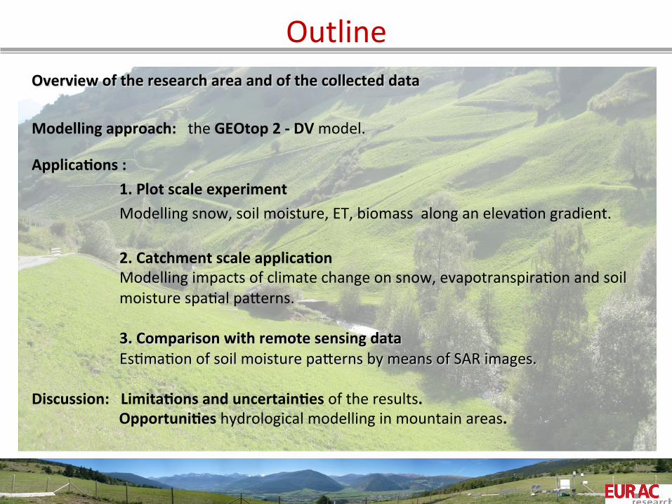
Matsch/Mazia, Vinschgau, South Tyrol, Italy
3
Area: ca. 100 km2. AlOtudinal range: 920– 3738 m a.s.l. Mean annual precipitaOon
(Mazia, 1580 m a.s.l.): 525 mm
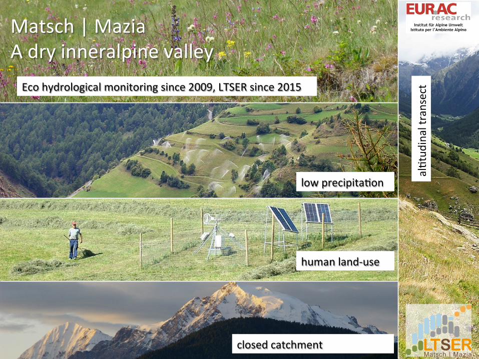
Matsch | Mazia A dry inneralpine valley
4
low precipitaOon
human land-‐use
closed catchment
alOtud
inal transect Eco hydrological monitoring since 2009, LTSER since 2015

Research topics
5
climate change & elevation
evapotranspiration soil moisture dynamics
water and runoff
agriculture productivity
land use change ecosystem services
biodiversity
snow and ice
grasslands and forest ecosystems
Alps
Ecosystem
Plot
Global
Future History Present
Region
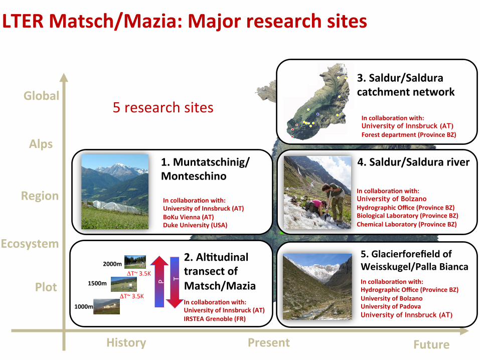
5 research sites
4. Saldur/Saldura river
3. Saldur/Saldura catchment network
5. Glacierforefield of Weisskugel/Palla Bianca
1. Muntatschinig/ Monteschino
In collabora=on with: University of Bolzano Hydrographic Office (Province BZ) Biological Laboratory (Province BZ) Chemical Laboratory (Province BZ)
In collabora=on with: Hydrographic Office (Province BZ) University of Bolzano University of Padova University of Innsbruck (AT)
In collabora=on with: University of Innsbruck (AT) BoKu Vienna (AT) Duke University (USA)
In collabora=on with: University of Innsbruck (AT) Forest department (Province BZ)
LTER Matsch/Mazia: Major research sites
2. Al=tudinal transect of Matsch/Mazia In collabora=on with: University of Innsbruck (AT) IRSTEA Grenoble (FR)
2000m
1500m
1000m
ΔT~ 3.5K
ΔT~ 3.5K
T P
Matsch | Mazia 7
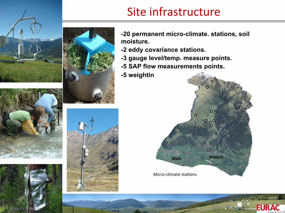
-20 permanent micro-climate. stations, soil moisture. -2 eddy covariance stations. -3 gauge level/temp. measure points. -5 SAP flow measurements points. -5 weighting lysimeters
Site infrastructure
Micro-‐climate staOons
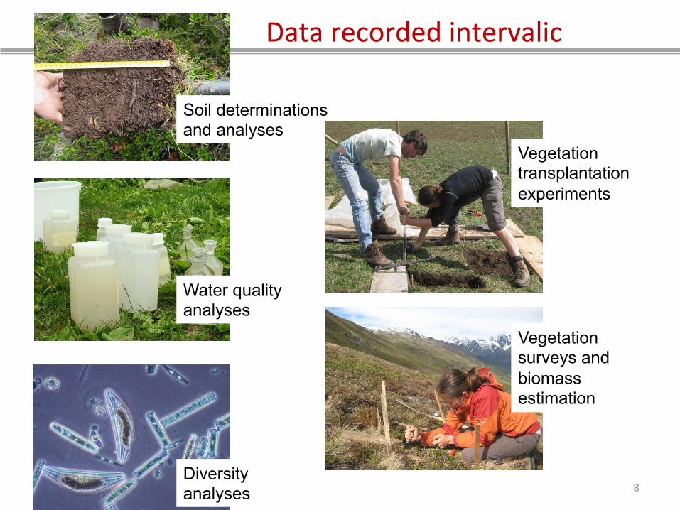
Data recorded intervalic
8
Soil determinations and analyses
Water quality analyses
Vegetation transplantation experiments
Vegetation surveys and biomass estimation
Diversity analyses
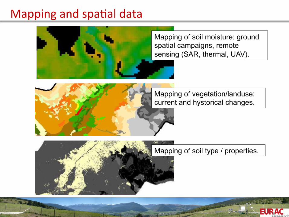
Mapping and spaOal data
Mapping of soil moisture: ground spatial campaigns, remote sensing (SAR, thermal, UAV).
Mapping of vegetation/landuse: current and hystorical changes.
Mapping of soil type / properties.
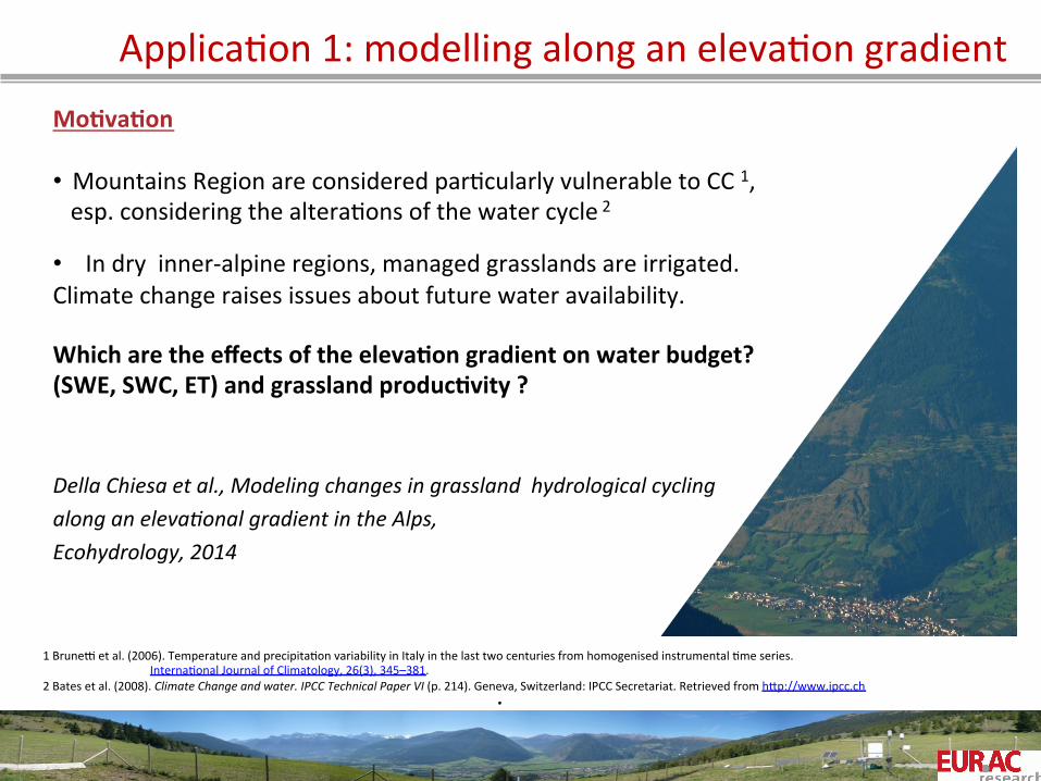
ApplicaOon 1: modelling along an elevaOon gradient Mo=va=on • Mountains Region are considered parOcularly vulnerable to CC 1, esp. considering the alteraOons of the water cycle 2
• In dry inner-‐alpine regions, managed grasslands are irrigated. Climate change raises issues about future water availability. Which are the effects of the eleva=on gradient on water budget? (SWE, SWC, ET) and grassland produc=vity ? Della Chiesa et al., Modeling changes in grassland hydrological cycling along an eleva6onal gradient in the Alps, Ecohydrology, 2014
.
1 Bruneb et al. (2006). Temperature and precipitaOon variability in Italy in the last two centuries from homogenised instrumental Ome series. InternaOonal Journal of Climatology, 26(3), 345–381.
2 Bates et al. (2008). Climate Change and water. IPCC Technical Paper VI (p. 214). Geneva, Switzerland: IPCC Secretariat. Retrieved from hPp://www.ipcc.ch
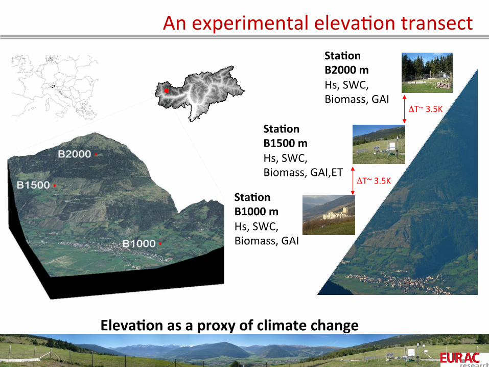
An experimental elevaOon transect
Eleva=on as a proxy of climate change
Sta=on B2000 m Hs, SWC, Biomass, GAI
Sta=on B1500 m Hs, SWC, Biomass, GAI,ET
Sta=on B1000 m Hs, SWC, Biomass, GAI
ΔT~ 3.5K
ΔT~ 3.5K

The GEOtop 2.0 – DV model
€
LW a tm↓ V
€
D0V
€
I
€
LW s ur r↓ 1−V( )
€
SWs ur r↓ 1−V( )
€
εsσTs4
Short waveradiat io n ( yell ow )Lo ngwave radiat io n( red )
€
SW r ef l
Complex topography
Bertoldi et al., J of Hydromet, 2006.
s Snow module
Endrizzi et al., GMDD, 2014 Zanob et al., Hydrol Proc, 2004
Water budget
Rigon et al., J of Hydromet, 2006.
Figures adapted from VIC model (Liang et al., 1994)
Energy budget
Bertoldi al., Ecohydrol, 2010.
Vegeta=on dynamics
Della Chiesa et al., Ecohydrol., 2014
From SHE model (Abbot et al., 1986)
TRIBS-‐VEGGIE FaOchi et al., 2012 Montaldo et al., 2005 Eagleson, 2002
Alpine3D, Lenhing et al., 2006 CROCUS, Brun et al., 1992 SNTHERM, Jordan, 1991
CLM, Dai et al., 2003 SEWAB, Megelkamp et al., 1999 Noah LSM, Chen et al., 1996, LSM, Bonan, 1996 BATS, Dickinson et al., 1986,
Corripio, 2010. Erbs et al., 1983. Iqbal, 1981.
tRIBS, Ivanov et al, 2004 Cailow, Zehe et al., 2001 InHM, VanderKwaak, and Loague, 2001 WaSim-‐ETH, Shulla 1997 Hydrogeosphere, Therrien and Sudicki, 1996 Parflow, Asby an Falgout, 1996 Cathy, Paniconi and Pub, 1994 DHSVM, Wigmosta et al., 1994 SHE, Abbot et al. 1986 Freeze and Harlan, 1969
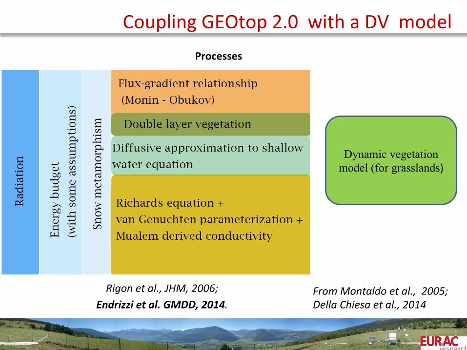
Coupling GEOtop 2.0 with a DV model
Rigon et al., JHM, 2006; Endrizzi et al. GMDD, 2014.
Processes
Dynamic vegetation model (for grasslands)
From Montaldo et al., 2005; Della Chiesa et al., 2014
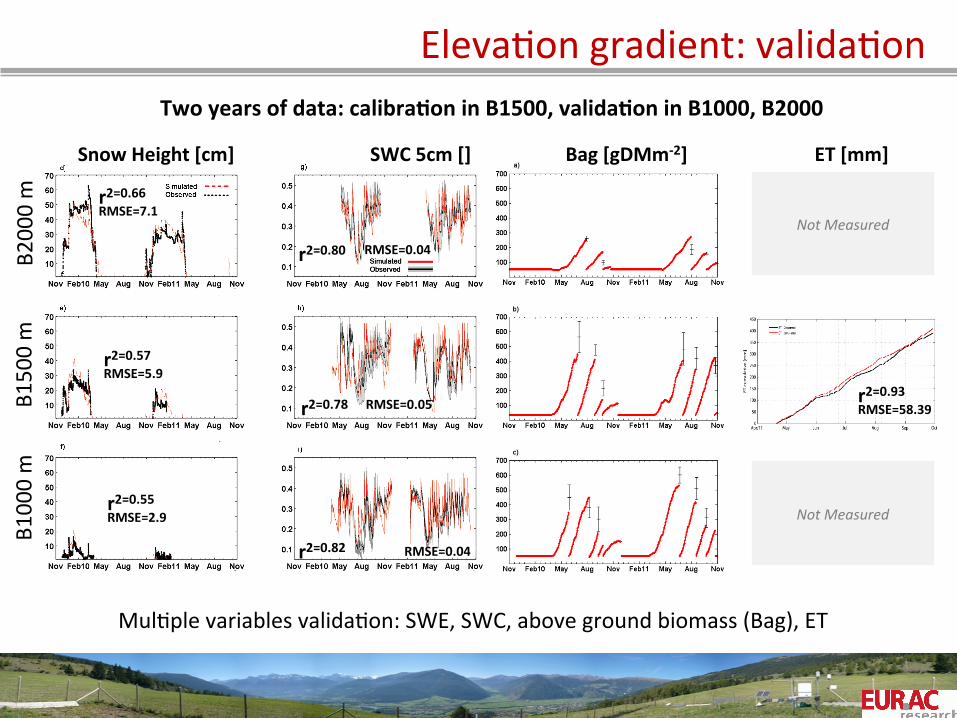
ElevaOon gradient: validaOon
MulOple variables validaOon: SWE, SWC, above ground biomass (Bag), ET
Two years of data: calibra=on in B1500, valida=on in B1000, B2000
B200
0 m
B150
0 m
B100
0 m
Snow Height [cm] SWC 5cm [] ET [mm]
Not Measured
Not Measured
r2=0.66 RMSE=7.1
r2=0.57 RMSE=5.9
r2=0.55 RMSE=2.9
r2=0.80
r2=0.78
r2=0.82
Bag [gDMm-‐2]
RMSE=0.04
RMSE=0.05
RMSE=0.04
r2=0.93 RMSE=58.39
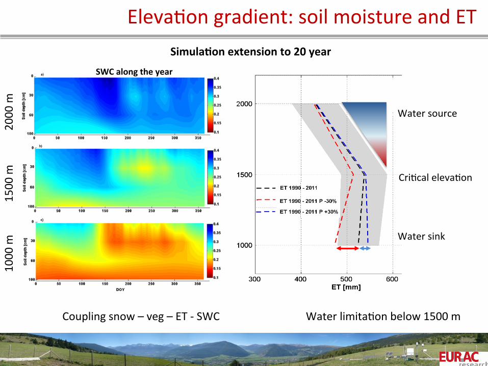
Simula=on extension to 20 year
Coupling snow – veg – ET -‐ SWC Water limitaOon below 1500 m
SWC along the year
SWC []
2000 m
1500 m
1000 m
SWC along the year
Water source
Water sink
CriOcal elevaOon
ElevaOon gradient: soil moisture and ET
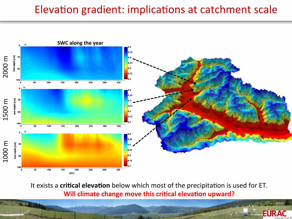
ElevaOon gradient: implicaOons at catchment scale
It exists a cri=cal eleva=on below which most of the precipitaOon is used for ET. Will climate change move this cri=cal eleva=on upward?
2000 m
1500 m
1000 m
SWC along the year
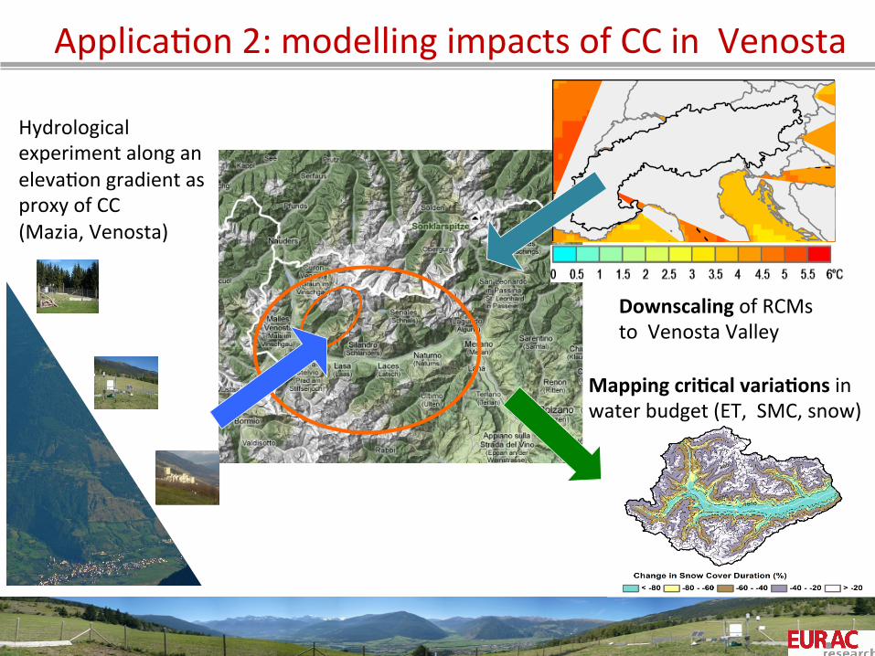
ApplicaOon 2: modelling impacts of CC in Venosta
Downscaling of RCMs to Venosta Valley
Mapping cri=cal varia=ons in water budget (ET, SMC, snow)
Hydrological experiment along an elevaOon gradient as proxy of CC (Mazia, Venosta)
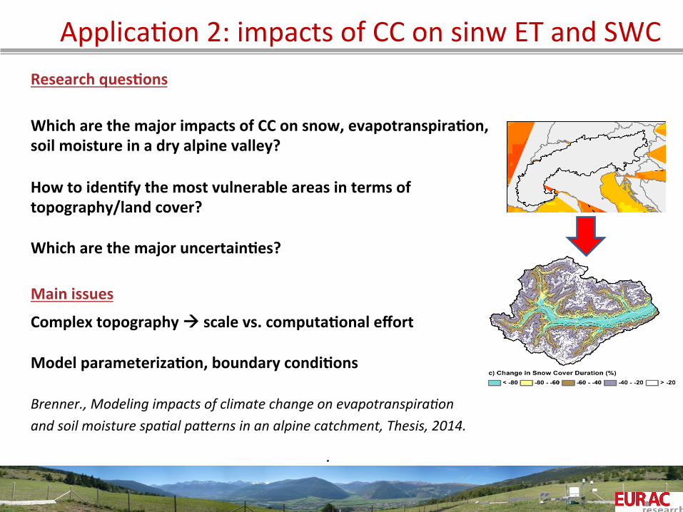
ApplicaOon 2: impacts of CC on sinw ET and SWC Research ques=ons
Which are the major impacts of CC on snow, evapotranspira=on, soil moisture in a dry alpine valley? How to iden=fy the most vulnerable areas in terms of topography/land cover? Which are the major uncertain=es? Main issues
Complex topography à scale vs. computa=onal effort Model parameteriza=on, boundary condi=ons Brenner., Modeling impacts of climate change on evapotranspira6on and soil moisture spa6al paTerns in an alpine catchment, Thesis, 2014.
.
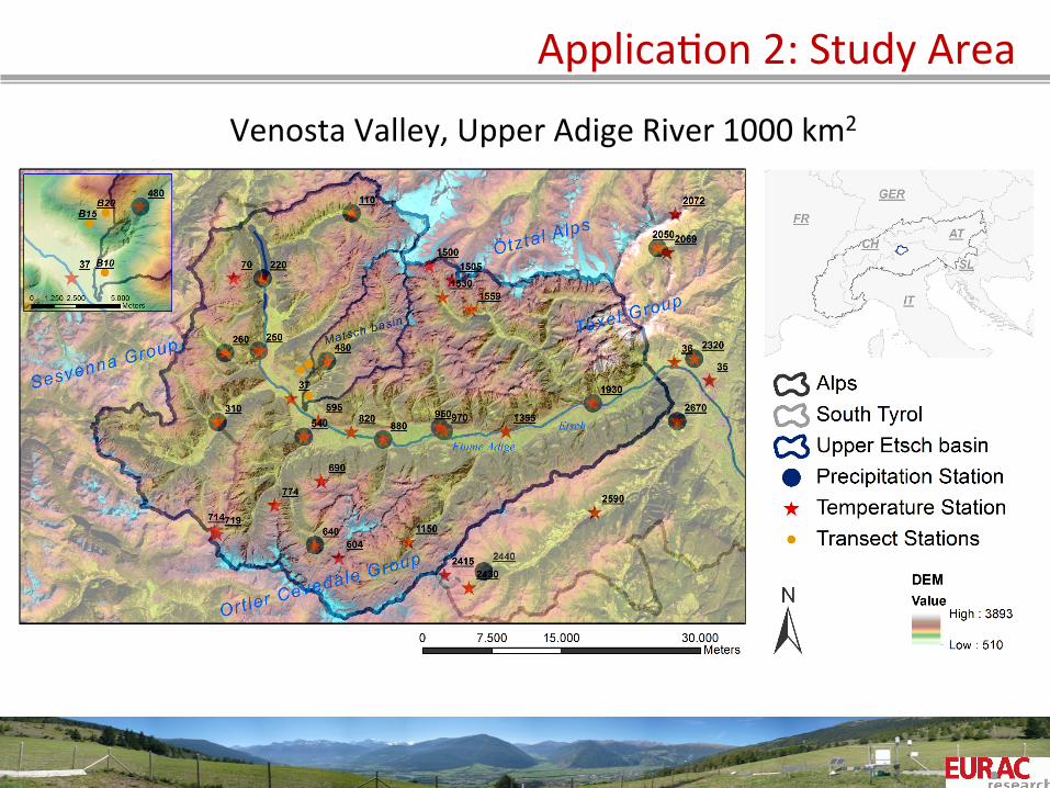
ApplicaOon 2: Study Area
Venosta Valley, Upper Adige River 1000 km2
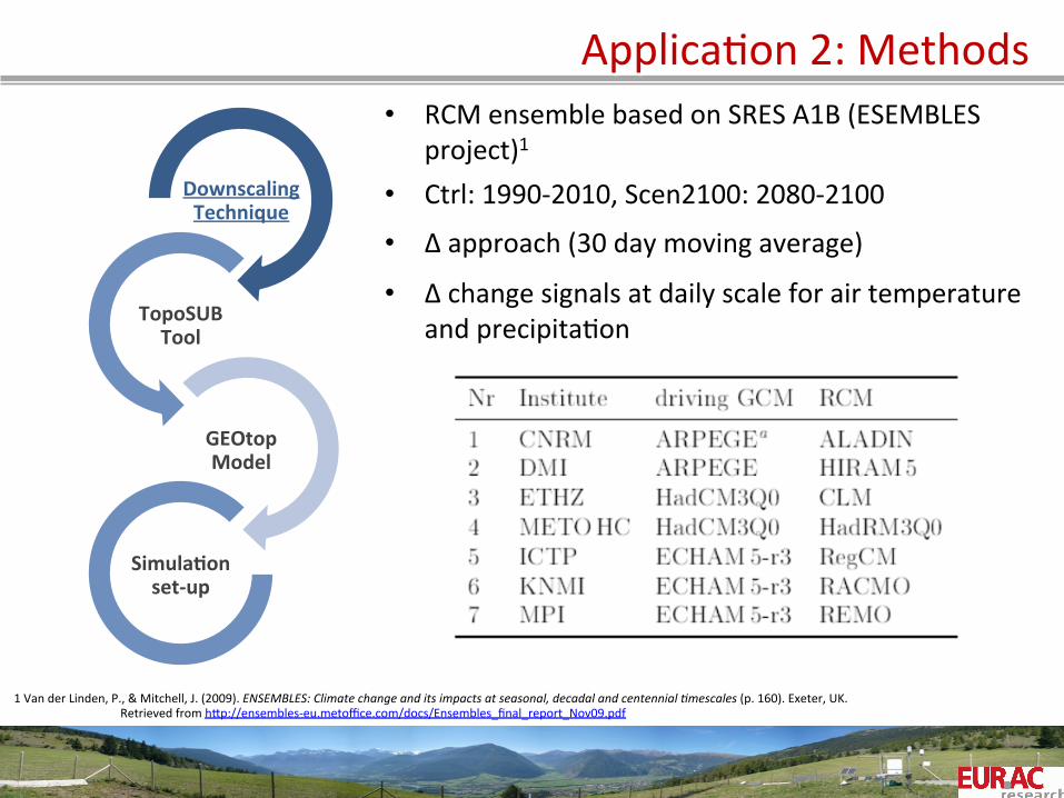
• RCM ensemble based on SRES A1B (ESEMBLES
project)1
• Ctrl: 1990-‐2010, Scen2100: 2080-‐2100
• ∆ approach (30 day moving average)
• ∆ change signals at daily scale for air temperature and precipitaOon
Downscaling Technique
TopoSUB Tool
GEOtop Model
Simula=on set-‐up
1 Van der Linden, P., & Mitchell, J. (2009). ENSEMBLES: Climate change and its impacts at seasonal, decadal and centennial 6mescales (p. 160). Exeter, UK. Retrieved from hPp://ensembles-‐eu.metoffice.com/docs/Ensembles_final_report_Nov09.pdf
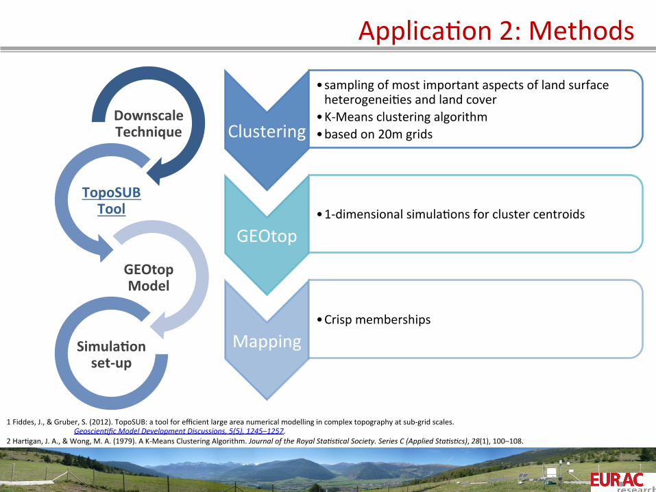
ApplicaOon 2: Methods
Downscale Technique
TopoSUB Tool
GEOtop Model
Simula=on set-‐up
1 Fiddes, J., & Gruber, S. (2012). TopoSUB: a tool for efficient large area numerical modelling in complex topography at sub-‐grid scales. Geoscien6fic Model Development Discussions, 5(5), 1245–1257.
2 HarOgan, J. A., & Wong, M. A. (1979). A K-‐Means Clustering Algorithm. Journal of the Royal Sta6s6cal Society. Series C (Applied Sta6s6cs), 28(1), 100–108.
Clustering
• sampling of most important aspects of land surface heterogeneiOes and land cover
• K-‐Means clustering algorithm 2 • based on 20m grids
GEOtop • 1-‐dimensional simulaOons for cluster centroids
Mapping • Crisp memberships
ApplicaOon 2: Methods
Downscale Technique
TopoSUB Tool
GEOtop Model
Simula=on set-‐up
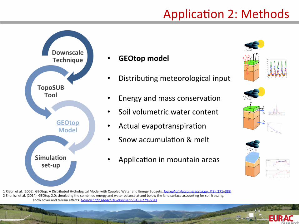
• GEOtop model
• DistribuOng meteorological input
• Energy and mass conservaOon
• Soil volumetric water content
• Actual evapotranspiraOon
• Snow accumulaOon & melt • ApplicaOon in mountain areas
1 Rigon et al. (2006). GEOtop: A Distributed Hydrological Model with Coupled Water and Energy Budgets. Journal of Hydrometeorology, 7(3), 371–388. 2 Endrizzi et al. (2014). GEOtop 2.0: simulaOng the combined energy and water balance at and below the land surface accounOng for soil freezing, snow cover and terrain effects. Geoscien6fic Model Development 6(4), 6279–6341.
ApplicaOon 2: Methods
Downscale Technique
TopoSUB Tool
GEOtop Model
Simula=on set-‐up
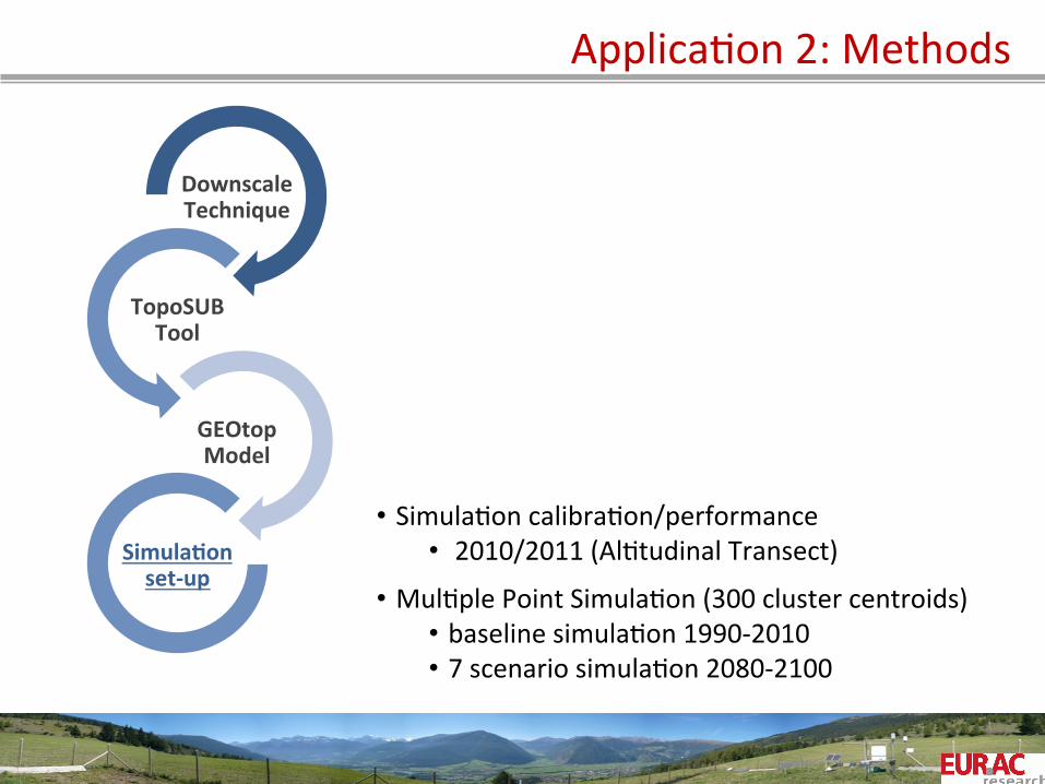
• SimulaOon calibraOon/performance • 2010/2011 (AlOtudinal Transect)
• MulOple Point SimulaOon (300 cluster centroids) • baseline simulaOon 1990-‐2010 • 7 scenario simulaOon 2080-‐2100
ApplicaOon 2: Methods
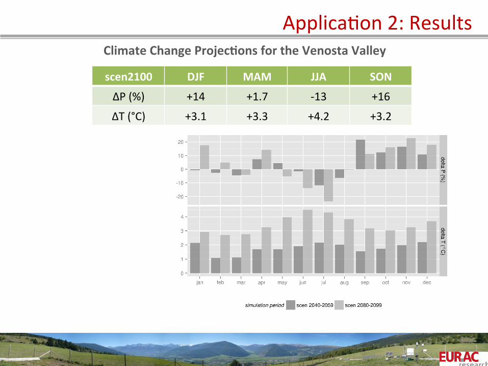
scen2100 DJF MAM JJA SON
∆P (%) +14 +1.7 -‐13 +16
∆T (°C) +3.1 +3.3 +4.2 +3.2
ApplicaOon 2: Results Climate Change Projec=ons for the Venosta Valley
Baseline SimulaOon ∆% (scen2100-‐ctrl)
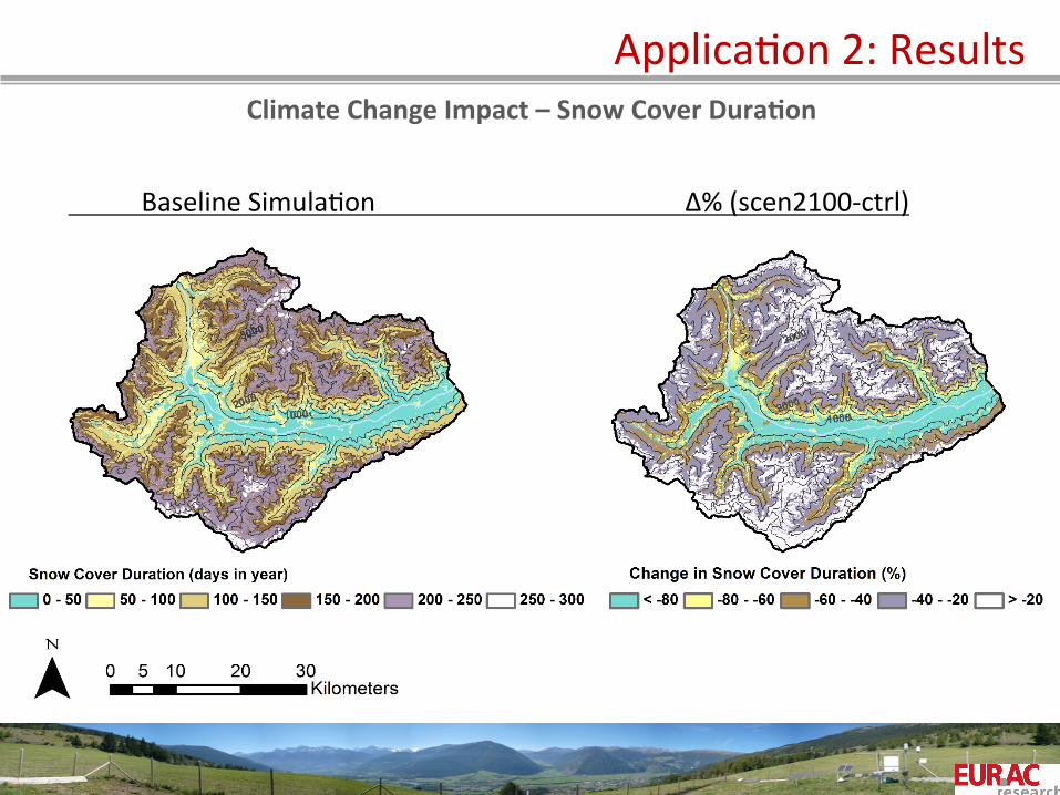
ApplicaOon 2: Results Climate Change Impact – Snow Cover Dura=on
Baseline SimulaOon ∆abs (scen2100-‐ctrl)
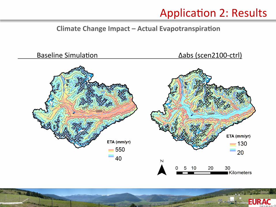
ApplicaOon 2: Results Climate Change Impact – Actual Evapotranspira=on

∆abs (scen2100-‐ctrl)
Change in M
ean An
nual ETA
(mm)
Aspect
Forest: South-‐east Major impact
Pasture: East
Bare Soil: South-‐east
Grassland & Agriculture: No effect of aspect
ApplicaOon 2: Results Climate Change Impact – Actual Evapotranspira=on
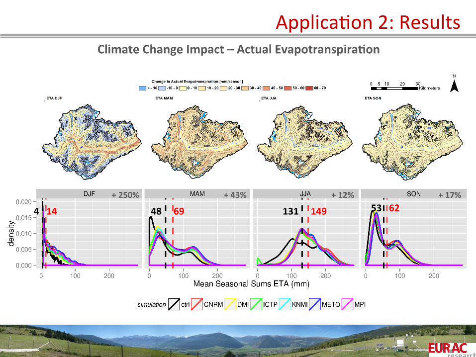
ApplicaOon 2: Results Climate Change Impact – Actual Evapotranspira=on
4 14 + 250%
48 69 + 43%
131 149 + 12%
53 62 + 17%
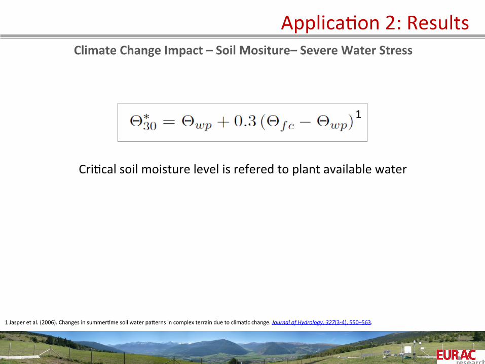
ApplicaOon 2: Results Climate Change Impact – Soil Mositure– Severe Water Stress
CriOcal soil moisture level is refered to plant available water
1
1 Jasper et al. (2006). Changes in summerOme soil water paPerns in complex terrain due to climaOc change. Journal of Hydrology, 327(3-‐4), 550–563.
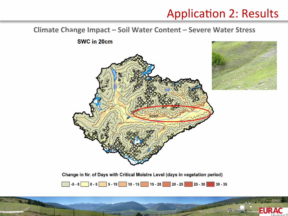
ApplicaOon 2: Results Climate Change Impact – Soil Water Content – Severe Water Stress
ApplicaOon 2: Conclusions
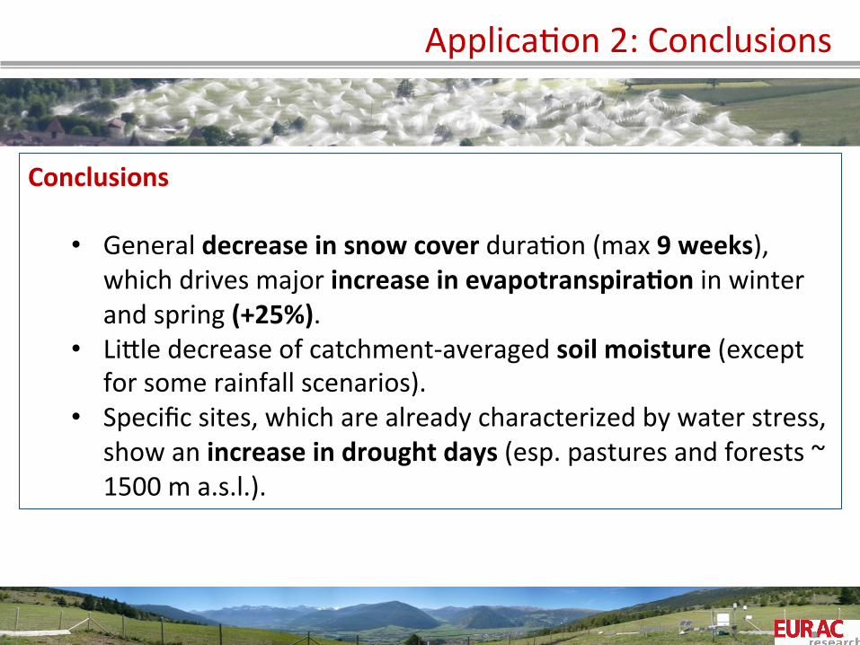
Conclusions
• General decrease in snow cover duraOon (max 9 weeks), which drives major increase in evapotranspira=on in winter and spring (+25%).
• LiPle decrease of catchment-‐averaged soil moisture (except for some rainfall scenarios).
• Specific sites, which are already characterized by water stress, show an increase in drought days (esp. pastures and forests ~ 1500 m a.s.l.).
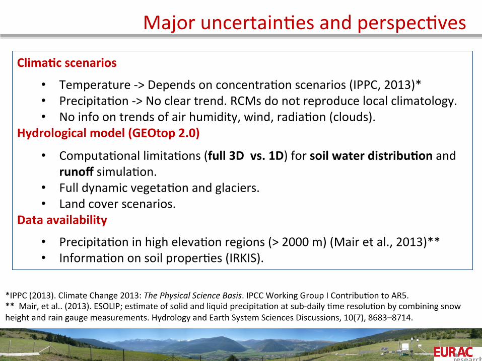
Major uncertainOes and perspecOves
Clima=c scenarios
• Temperature -‐> Depends on concentraOon scenarios (IPPC, 2013)* • PrecipitaOon -‐> No clear trend. RCMs do not reproduce local climatology. • No info on trends of air humidity, wind, radiaOon (clouds).
Hydrological model (GEOtop 2.0)
• ComputaOonal limitaOons (full 3D vs. 1D) for soil water distribu=on and runoff simulaOon.
• Full dynamic vegetaOon and glaciers. • Land cover scenarios.
Data availability
• PrecipitaOon in high elevaOon regions (> 2000 m) (Mair et al., 2013)** • InformaOon on soil properOes (IRKIS).
*IPPC (2013). Climate Change 2013: The Physical Science Basis. IPCC Working Group I ContribuOon to AR5. ** Mair, et al.. (2013). ESOLIP; esOmate of solid and liquid precipitaOon at sub-‐daily Ome resoluOon by combining snow height and rain gauge measurements. Hydrology and Earth System Sciences Discussions, 10(7), 8683–8714.
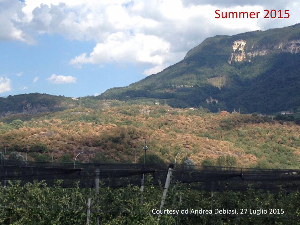
Summer 2015
Courtesy od Andrea Debiasi, 27 Luglio 2015
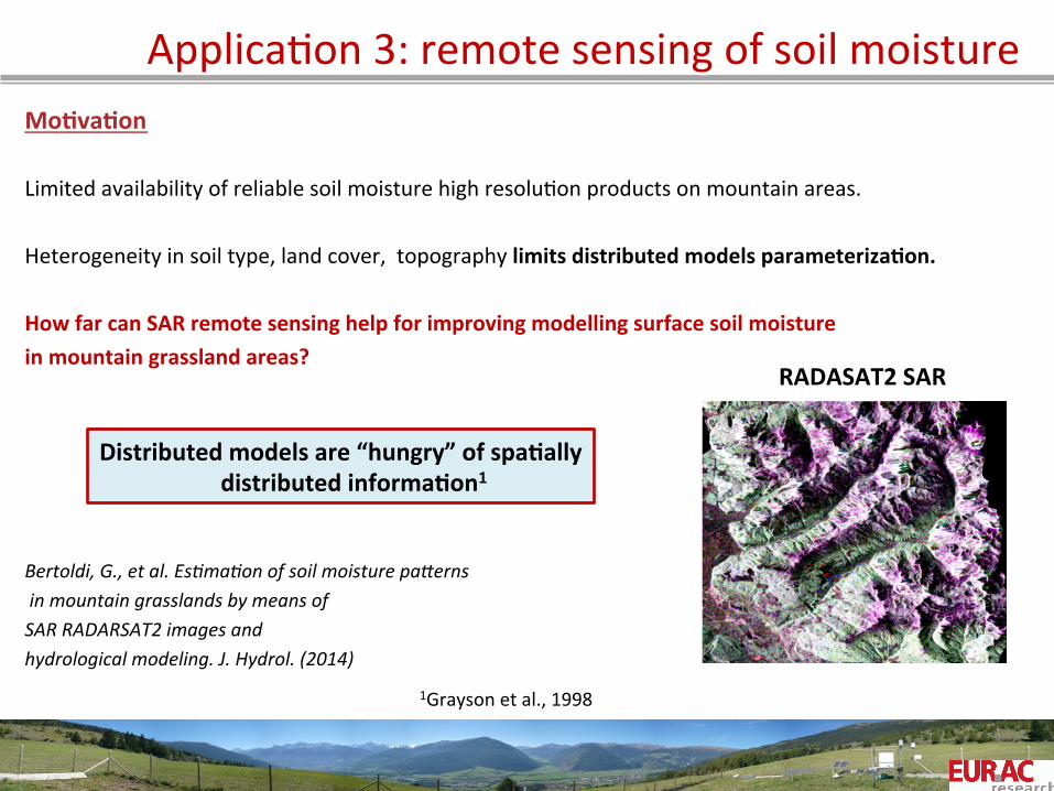
ApplicaOon 3: remote sensing of soil moisture Mo=va=on Limited availability of reliable soil moisture high resoluOon products on mountain areas. Heterogeneity in soil type, land cover, topography limits distributed models parameteriza=on. How far can SAR remote sensing help for improving modelling surface soil moisture in mountain grassland areas?
Bertoldi, G., et al. Es6ma6on of soil moisture paTerns in mountain grasslands by means of SAR RADARSAT2 images and hydrological modeling. J. Hydrol. (2014)
RADASAT2 SAR
Distributed models are “hungry” of spa=ally distributed informa=on1
1Grayson et al., 1998
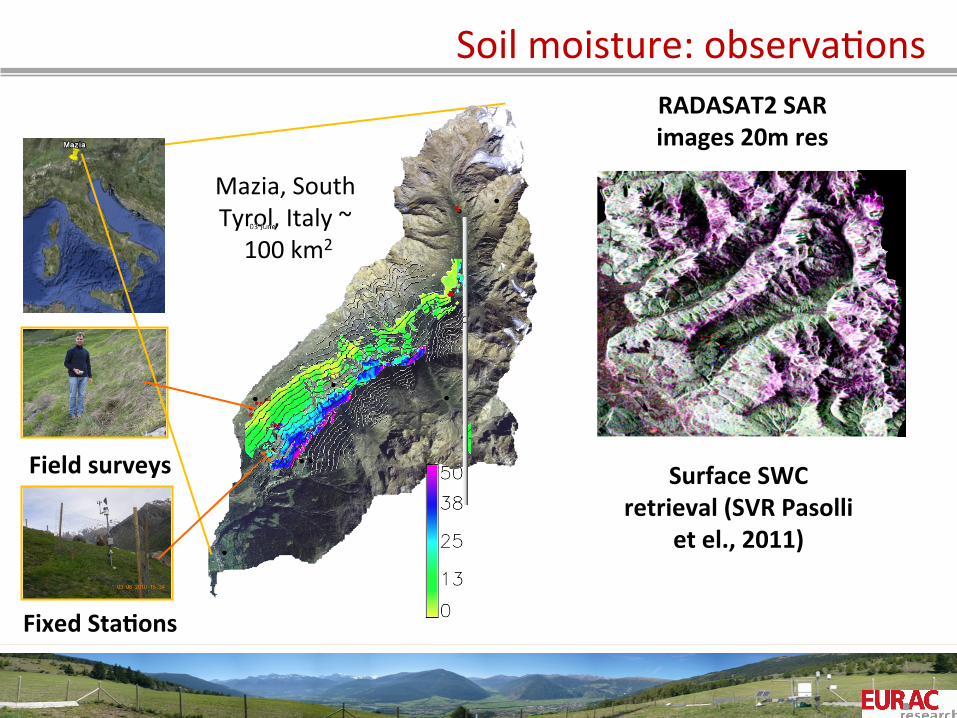
Soil moisture: observaOons
Fixed Sta=ons
Field surveys
Mazia, South Tyrol, Italy ~ 100 km2
RADASAT2 SAR images 20m res
Surface SWC retrieval (SVR Pasolli
et el., 2011)

Ground observaOons: mobile surveys
• Monitoring SMC spa=al paserns at hillslope scale; • Survey planned to map land cover/topographic features; • Good correspondence with staOon values.
• More than 10 surveys between 2010 and 2014; • More than 1000 points with mobile Delta-‐T wet sensor (TDR) 0 – 5 cm depth;
10 % 50 %
SWC
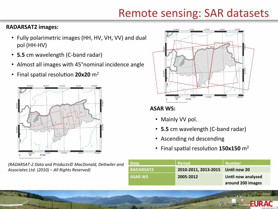
Remote sensing: SAR datasets RADARSAT2 images:
• Fully polarimetric images (HH, HV, VH, VV) and dual pol (HH-‐HV)
• 5.5 cm wavelength (C-‐band radar) • Almost all images with 45°nominal incidence angle
• Final spaOal resoluOon 20x20 m2
(RADARSAT-‐2 Data and Products© MacDonald, DeTwiler and Associates Ltd. (2010) – All Rights Reserved)
Data Period Number RADARSAT2 2010-‐2011, 2013-‐2015 Un=l now 20 ASAR WS 2005-‐2012 Un=l now analyzed
around 200 images
ASAR WS:
• Mainly VV pol. • 5.5 cm wavelength (C-‐band radar) • Ascending nd descending • Final spaOal resoluOon 150x150 m2
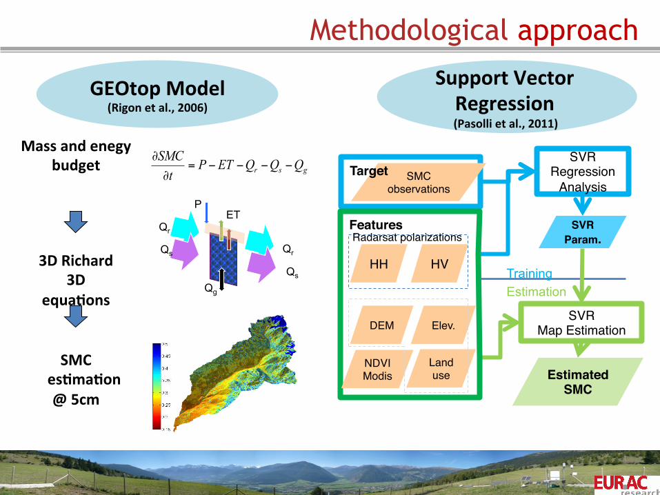
Methodological approach
GEOtop Model (Rigon et al., 2006)
Support Vector Regression (Pasolli et al., 2011)
gsr QQQETPt
SMC−−−−=
∂
∂
ET Qr
Qr Qs
Qs
Qg
P
Mass and enegy budget
3D Richard 3D
equa=ons
SMC es=ma=on @ 5cm
HH HV
NDVI Modis
Elev.DEM
Land use
Radarsat polarizationsFeatures
SMC observations
Target
SVRParam.
SVRRegression
Analysis
SVRMap Estimation
Estimated SMC
Estimation Training
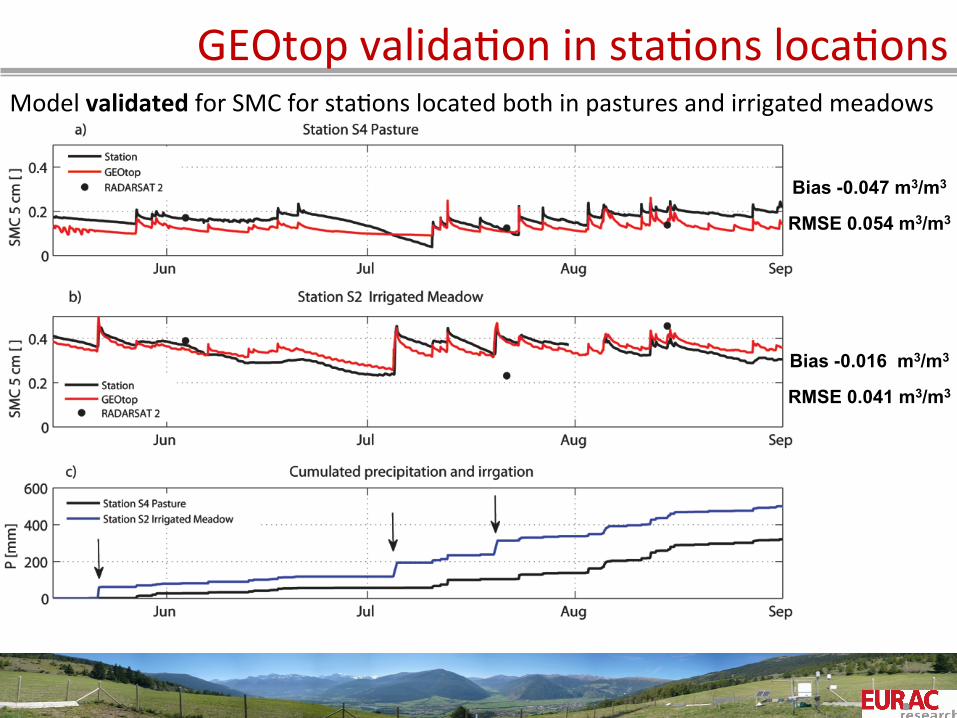
GEOtop validaOon in staOons locaOons Model validated for SMC for staOons located both in pastures and irrigated meadows
Bias -0.047 m3/m3
RMSE 0.054 m3/m3
Bias -0.016 m3/m3
RMSE 0.041 m3/m3
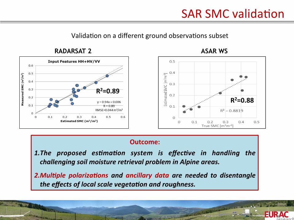
SAR SMC validaOon
Grassland Pasture Total
RMSE 4.05 1.68 2.68
R2 0.56 0.75 0.79
Slope 0.56 0.70 0.78
Intercept 7.15 2.3 2.26
Outcome: 1. The proposed es:ma:on system is effec:ve in handling the challenging soil moisture retrieval problem in Alpine areas.
2. Mul:ple polariza:ons and ancillary data are needed to disentangle the effects of local scale vegeta:on and roughness.
RADARSAT 2 ASAR WS
R2=0.89 R2=0.88
ValidaOon on a different ground observaOons subset
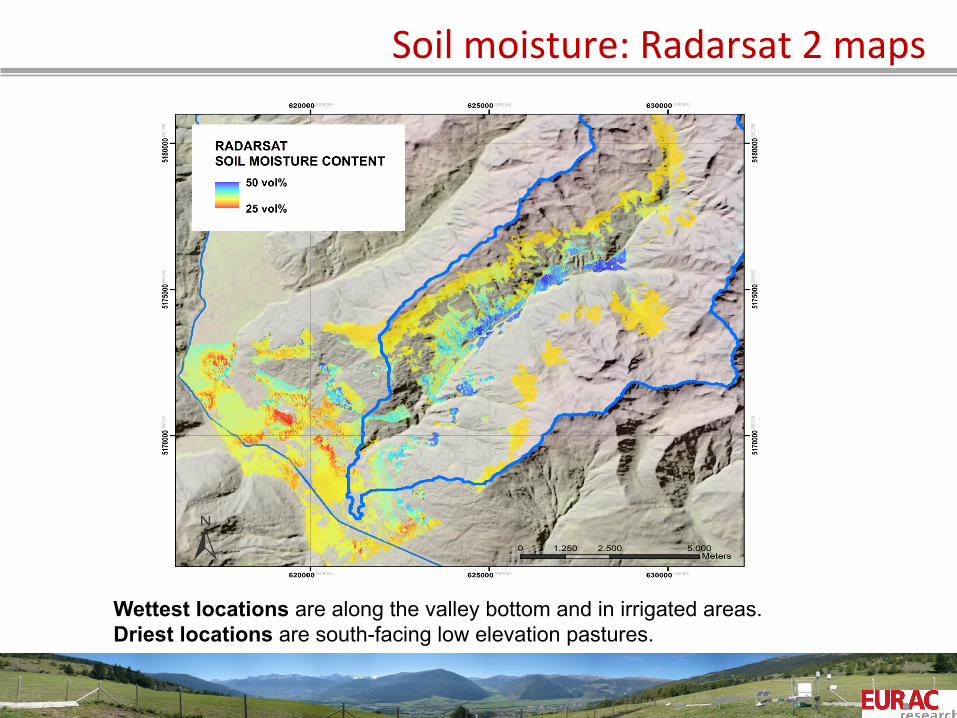
Soil moisture: Radarsat 2 maps
Wettest locations are along the valley bottom and in irrigated areas. Driest locations are south-facing low elevation pastures.
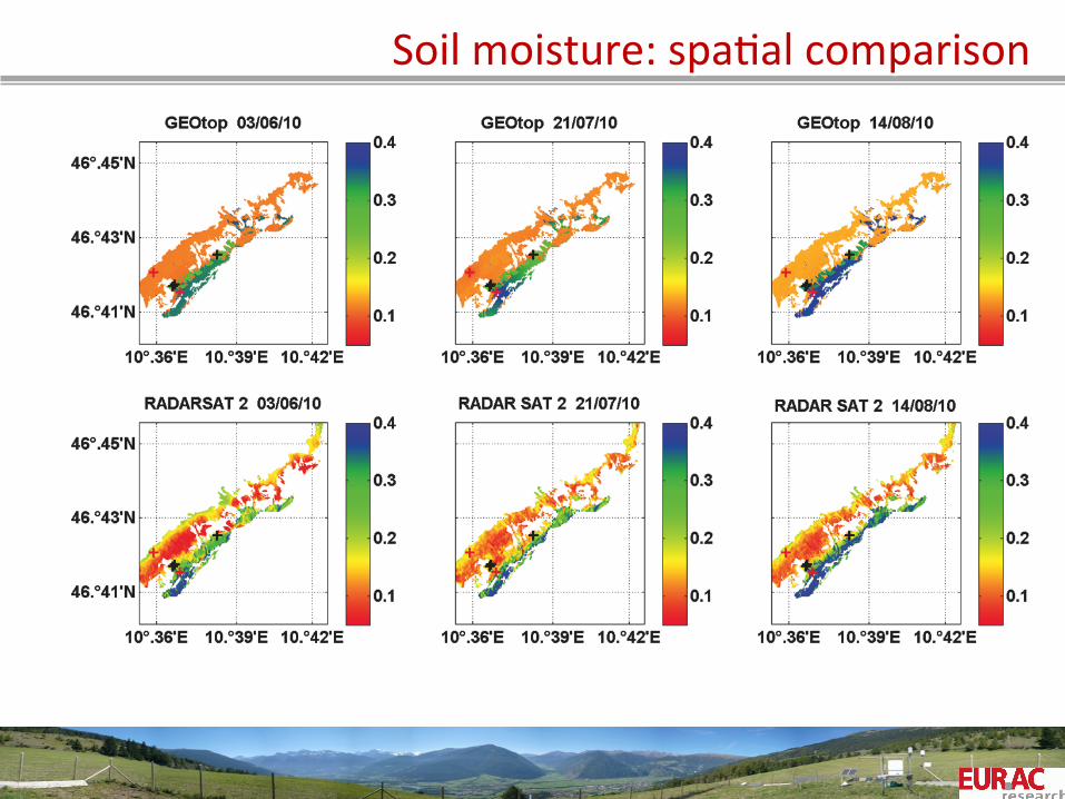
Soil moisture: spaOal comparison
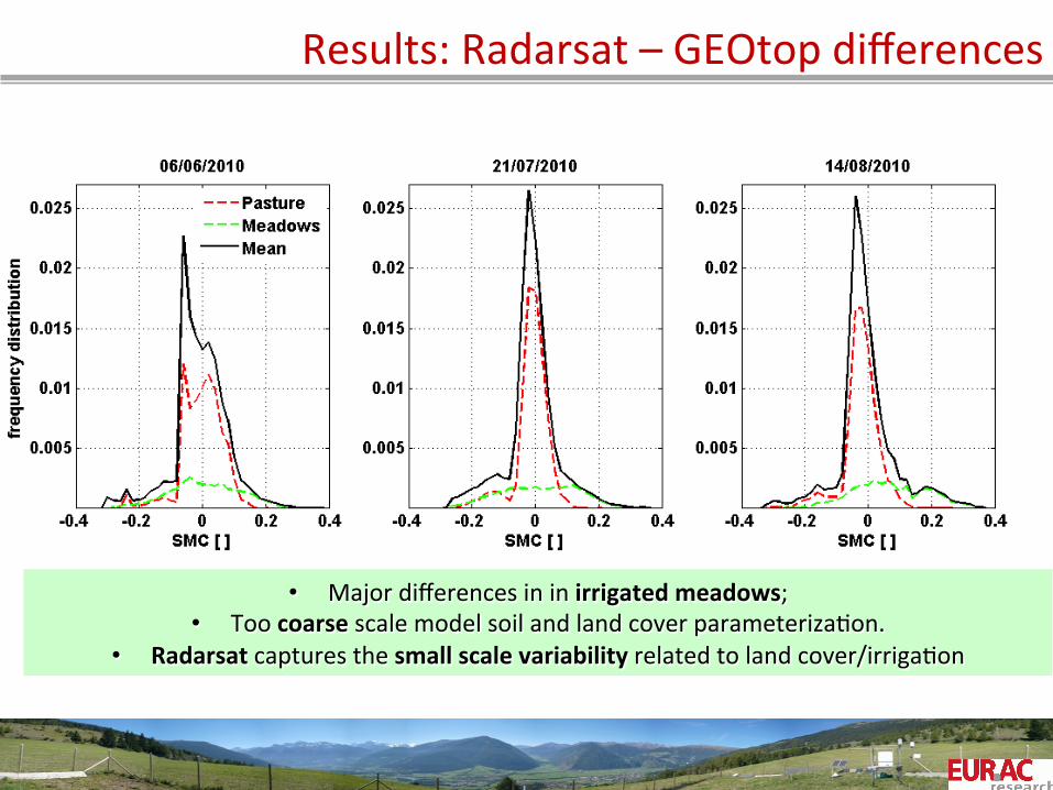
Results: Radarsat – GEOtop differences
• Major differences in in irrigated meadows; • Too coarse scale model soil and land cover parameterizaOon.
• Radarsat captures the small scale variability related to land cover/irrigaOon
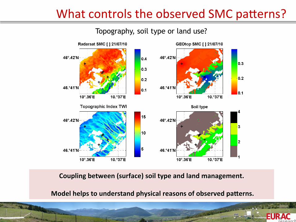
What controls the observed SMC paPerns?
Coupling between (surface) soil type and land management.
Model helps to understand physical reasons of observed paserns.
Topography, soil type or land use?
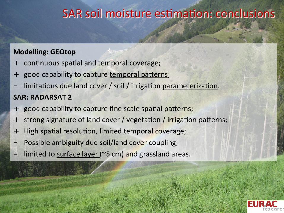
SAR soil moisture esOmaOon: conclusions
Modelling: GEOtop + conOnuous spaOal and temporal coverage; + good capability to capture temporal paPerns; - limitaOons due land cover / soil / irrigaOon parameterizaOon. SAR: RADARSAT 2 + good capability to capture fine scale spaOal paPerns; + strong signature of land cover / vegetaOon / irrigaOon paPerns; + High spaOal resoluOon, limited temporal coverage; - Possible ambiguity due soil/land cover coupling; - limited to surface layer (~5 cm) and grassland areas.
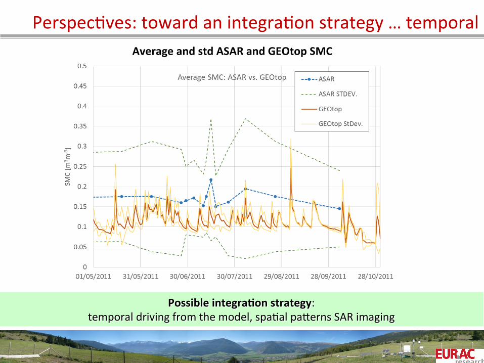
PerspecOves: toward an integraOon strategy … temporal
Possible integra=on strategy: temporal driving from the model, spaOal paPerns SAR imaging
Average and std ASAR and GEOtop SMC

Toward an integraOon strategy … spaOal
ASAR GEOtop
Use model-‐derived data as addiOonal input feature for a SVR approach in areas where limited ground truth is available.
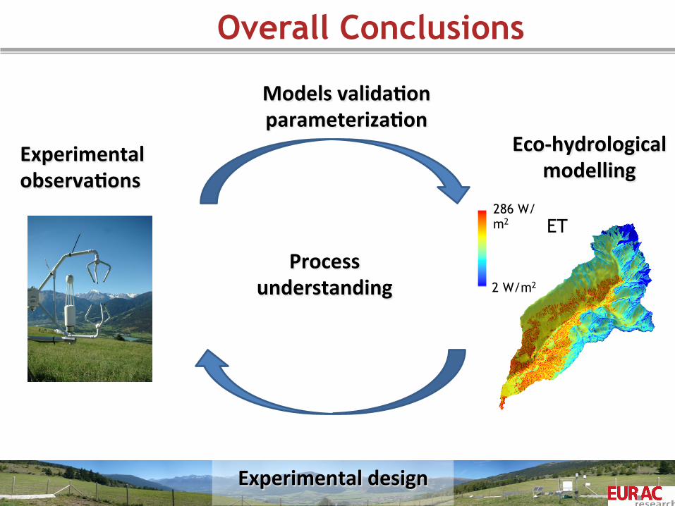
Overall Conclusions
Experimental observa=ons
Experimental design
Models valida=on parameteriza=on
Process understanding
Eco-‐hydrological modelling
ET
2 W/m2
286 W/m2
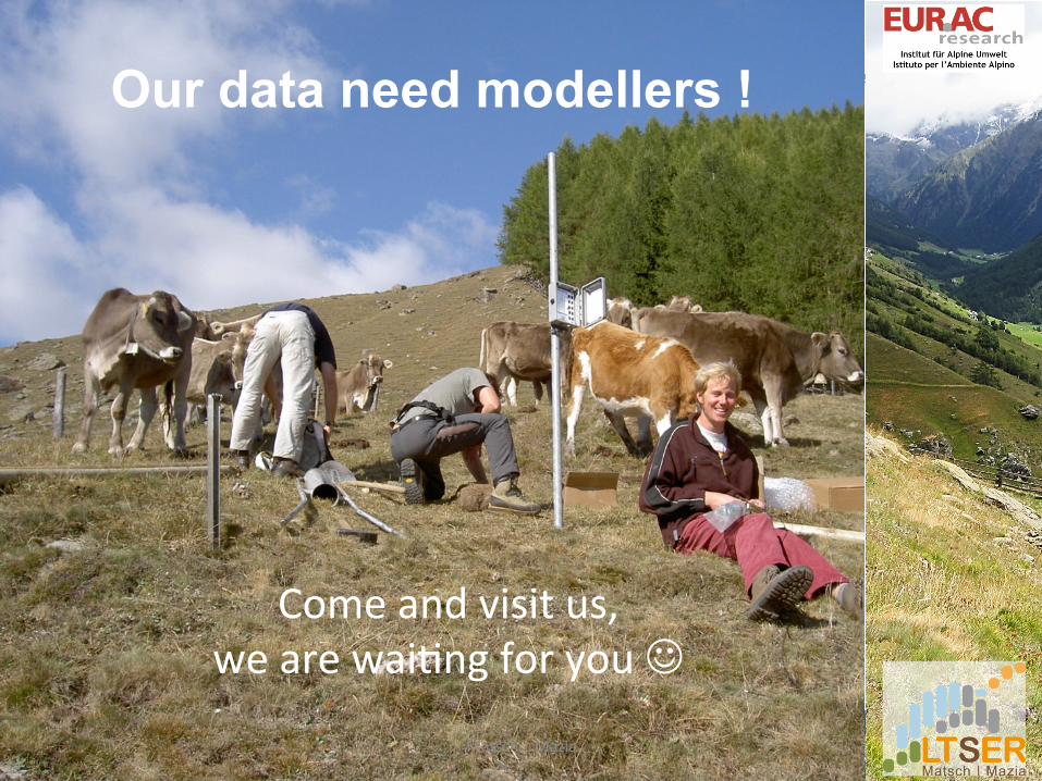
Come and visit us, we are waiOng for you J
Matsch | Mazia 49
Our data need modellers !
Acknowledgments
This study is supported by the projects “and “HydroAlp” and “HiResAlp” financed by Provincia Autonoma di Bolzano, Alto Adige, Ripar=zione Diriso allo sudio, Università e ricerca scien=fica.
We hereby would like to thank:
M. Dall´Amico, Mountaneering s.r.l. S. Endrizzi, University of Zurich. R. Rigon, University of Trento.
G. Wohlxart, University of Innsbruck
Thank you for your aGen:on!

Opportunites and challenges
Ø Using physically models in real contexts is someOmes more Ome-‐consuming than doing real experiments.
Ø A deep knowledge of the system is needed for set-‐up proper assumpOons in model parameterizaOon (a lot on unknown informaOon).
Ø Great tools for tesOng hypotheses and generalize results.
Opportunites and challenges
Ø The parOcularly dry area represents a unique chance to study climate change allowing predicOons of future climate on mountain ecosystems.
Ø The eleva=on transect allows for experimental and numerical invesOgaOon on effects of elevaOon on eco-‐hydrological processes.
Ø The site allows interdisciplinary observaOons of relevant eco-‐hydrological processes in a human-‐influenced mountain region.
Ø The climaOc condiOons of Val Mazia may allow interesOng comparisons among different mountain sites of the MRI / LTER network.
Ø Chance to be part of a well organized and good structured scien=fic network.
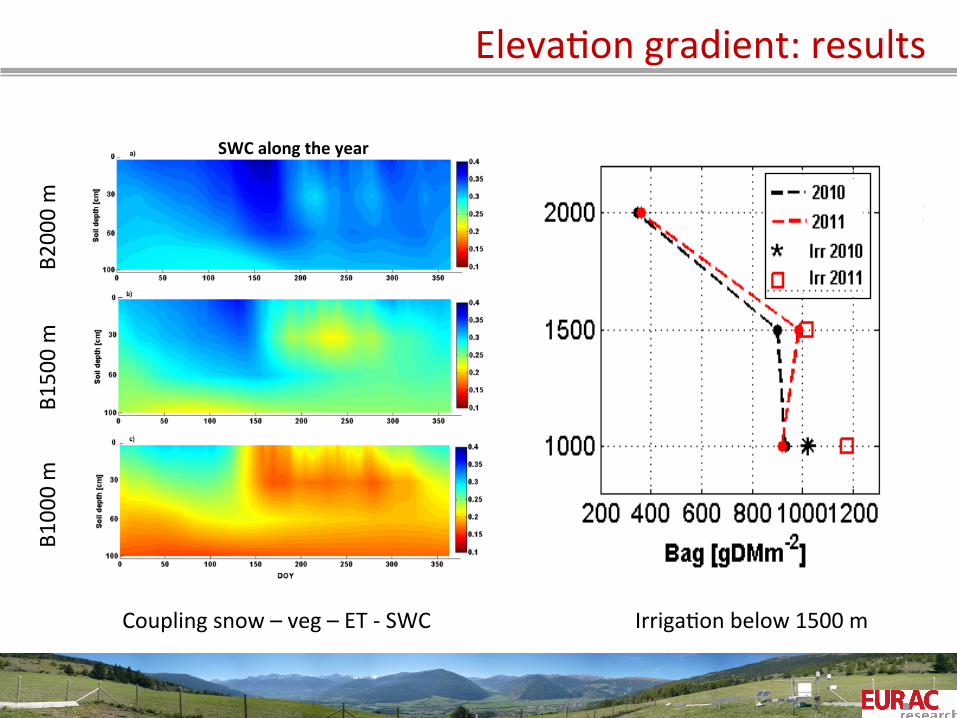
ElevaOon gradient: results B2
000 m
B150
0 m
B100
0 m
Coupling snow – veg – ET -‐ SWC
SWC along the year
IrrigaOon below 1500 m
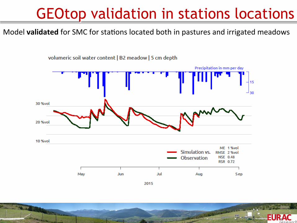
GEOtop validation in stations locations Model validated for SMC for staOons located both in pastures and irrigated meadows
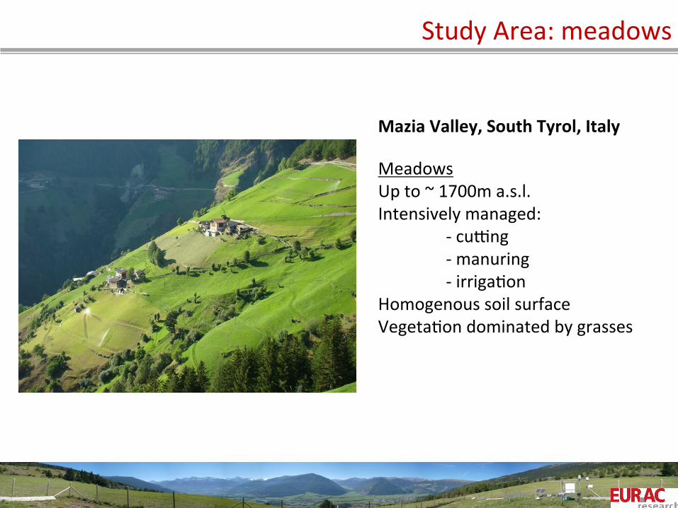
Study Area: meadows
57
Mazia Valley, South Tyrol, Italy Meadows Up to ~ 1700m a.s.l. Intensively managed:
-‐ cubng -‐ manuring -‐ irrigaOon
Homogenous soil surface VegetaOon dominated by grasses

Study Area: pastures
58
Mazia Valley, South Tyrol, Italy Pastures Located at 1700 to 2400m a.s.l. Steep terrain Heterogeneous soil surface:
-‐ bare soil -‐ stones -‐ large rocks
VegetaOon dominated by grasses

Study area: soil properOes
Kolmann and Tasser, 2012
• Two main soil types: 1. Haplic Leptosol (ranker) mainly in pastures; 2. Dystric Cambisol (braunerde) mainly in meadows (Kollman, M. Th., 2013).
• Observed soil parameters are in the typical range of loamy sand (Leptosoil) and sandy loam (Cambisoil).
Kollmann, K.. Klima-‐ und landnutzungsbedingte Bodenverteilung im Matschertal, SüdOrol. Ms. Thesis, Universität Innsbruck.(2012).
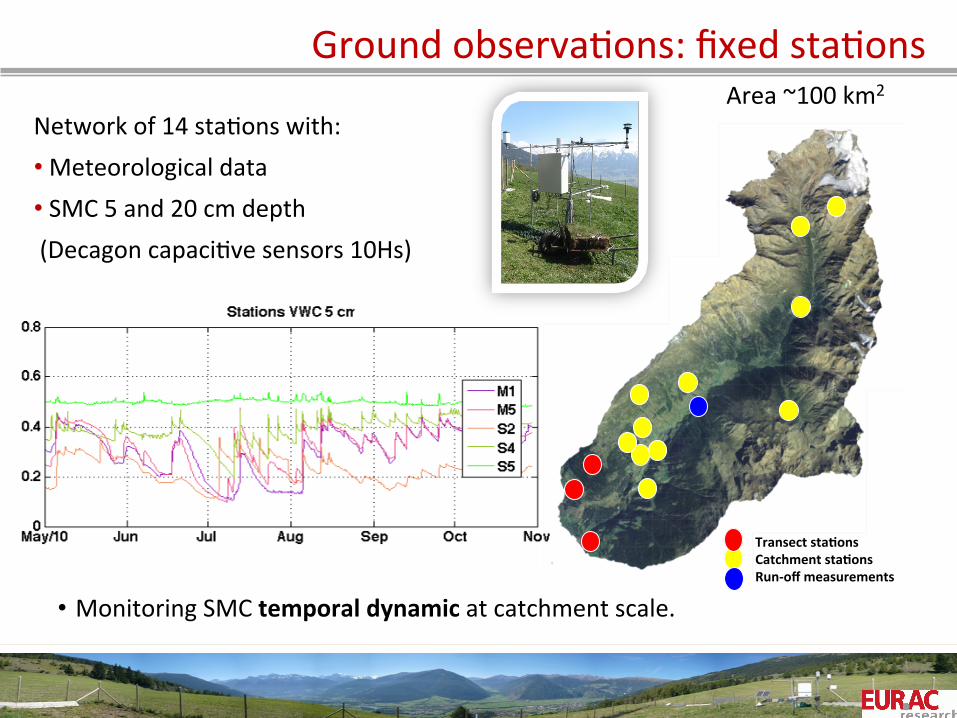
Ground observaOons: fixed staOons
Network of 14 staOons with: • Meteorological data • SMC 5 and 20 cm depth (Decagon capaciOve sensors 10Hs)
Transect sta=ons Catchment sta=ons Run-‐off measurements
Area ~100 km2
• Monitoring SMC temporal dynamic at catchment scale.

Ground observaOons: mobile surveys
• Monitoring SMC spa=al paserns at hillslope scale; • Survey planned to map land cover/topographic features; • Good correspondence with staOon values.
• More than 10 surveys between 2010 and 2014; • More than 1000 points with mobile Delta-‐T wet sensor (TDR) 0 – 5 cm depth;
10 % 50 %
SWC
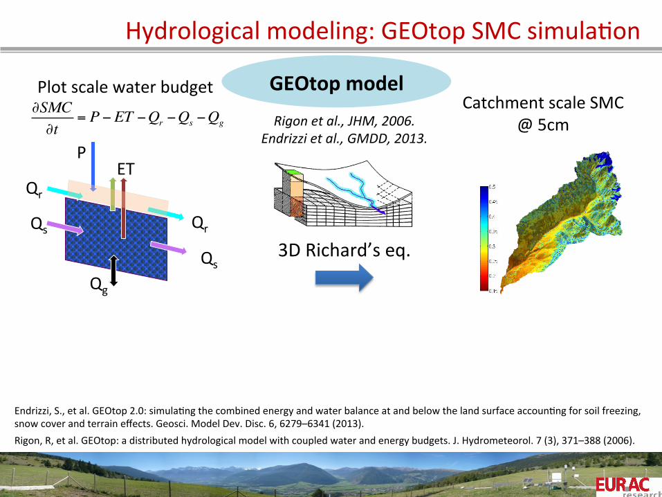
Hydrological modeling: GEOtop SMC simulaOon
GEOtop model
Rigon et al., JHM, 2006. Endrizzi et al., GMDD, 2013.
∂SMC∂t
= P −ET −Qr −Qs −Qg
ET Qr
Qr Qs
Qs
Qg
P
Plot scale water budget Catchment scale SMC
@ 5cm
3D Richard’s eq.
Endrizzi, S., et al. GEOtop 2.0: simulaOng the combined energy and water balance at and below the land surface accounOng for soil freezing, snow cover and terrain effects. Geosci. Model Dev. Disc. 6, 6279–6341 (2013). Rigon, R, et al. GEOtop: a distributed hydrological model with coupled water and energy budgets. J. Hydrometeorol. 7 (3), 371–388 (2006).
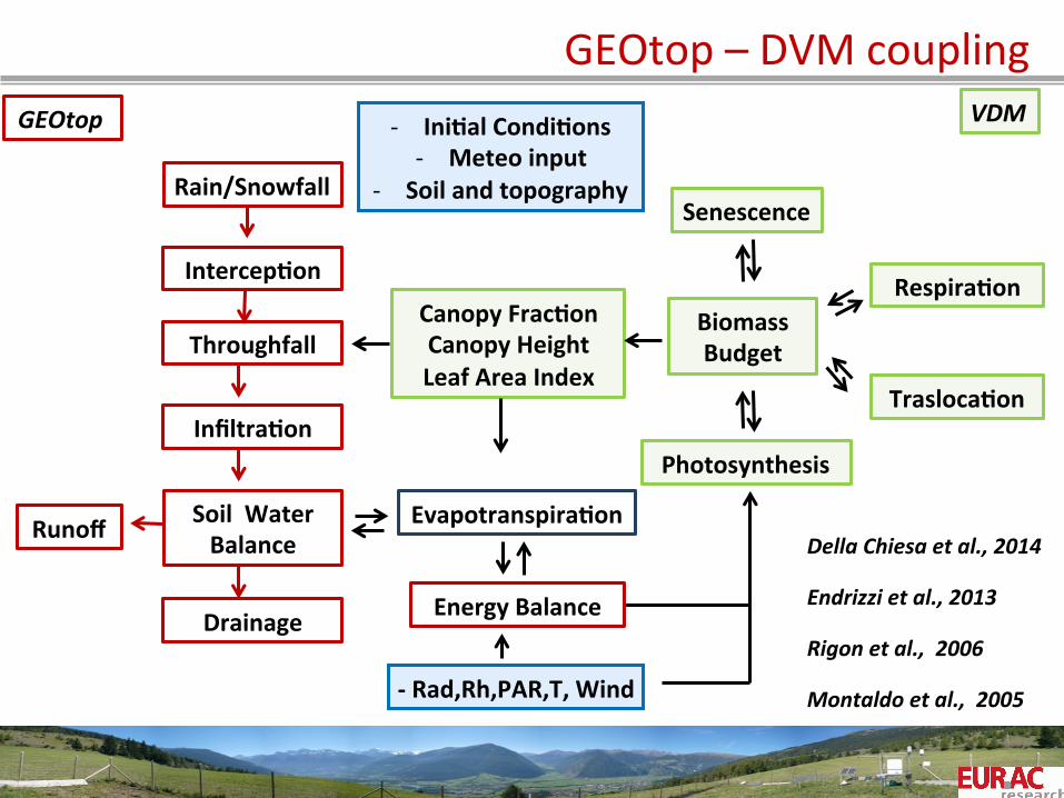
GEOtop – DVM coupling GEOtop VDM
-‐ Rad,Rh,PAR,T, Wind
-‐ Ini=al Condi=ons -‐ Meteo input
-‐ Soil and topography
Montaldo et al., 2005
Endrizzi et al., 2013
Canopy Frac=on Canopy Height Leaf Area Index
Senescence
Respira=on
Trasloca=on
Biomass Budget
Photosynthesis
Evapotranspira=on
Intercep=on
Energy Balance
Throughfall
Infiltra=on
Soil Water Balance Runoff
Drainage
Rain/Snowfall
Rigon et al., 2006
Della Chiesa et al., 2014
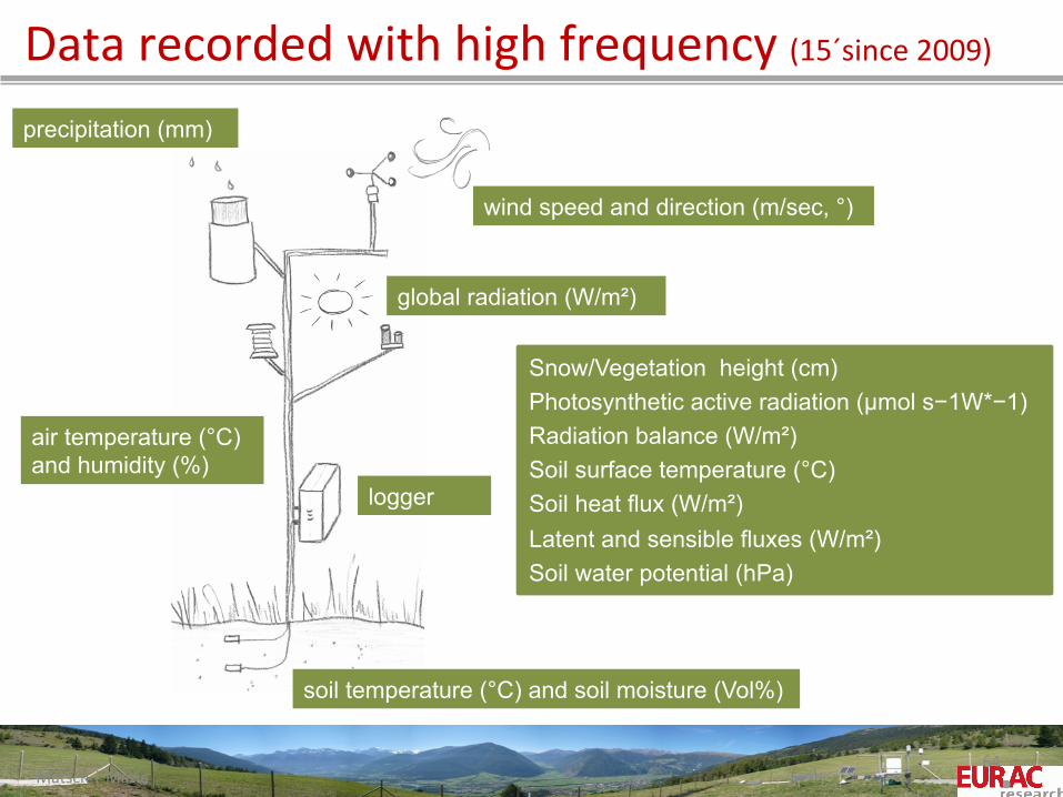
Data recorded with high frequency (15´since 2009)
Matsch | Mazia 64
precipitation (mm)
global radiation (W/m²)
soil temperature (°C) and soil moisture (Vol%)
logger
air temperature (°C) and humidity (%)
Snow/Vegetation height (cm) Photosynthetic active radiation (µmol s−1W*−1) Radiation balance (W/m²) Soil surface temperature (°C) Soil heat flux (W/m²) Latent and sensible fluxes (W/m²) Soil water potential (hPa)
wind speed and direction (m/sec, °)
Coupled ecohydrological modelling
How to use experimental observa=ons to validate a distributed ecohydrological models? How to use model results to improve our knowledge of the ecohydrological behavior of mountain catchments?
Top Related