


Languages
Pages
Legal


GEOPHYSICAL PROSPECTING
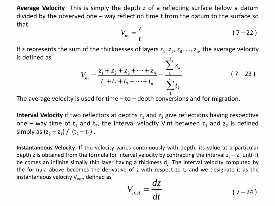
Average Velocity This is simply the depth z of a reflecting surface below a datumdivided by the observed one – way reflection time t from the datum to the surface sothat.
( 7 – 22 )
If z represents the sum of the thicknesses of layers z1, z2, z3, …, zn, the average velocityis defined as
( 7 – 23 )
The average velocity is used for time – to – depth conversions and for migration.
Interval Velocity if two reflectors at depths z1 and z2 give reflections having respectiveone – way time of t1 and t2, the interval velocity Vint between z1 and z2 is definedsimply as (z2 – z1) / (t2 – t1) .
Instantaneous Velocity. If the velocity varies continuously with depth, its value at a particulardepth z is obtained from the formula for interval velocity by contracting the interval z2 – z1 until itbe comes an infinite simally thin layer having a thickness dz. The interval velocity computed bythe formula above becomes the derivative of z with respect to t, and we designate it as theinstantaneous velocity Vinst, defined as
( 7 – 24 )
1 2 3 1
1 2 3
1
av
n
k
nav n
nk
zV
t
zz z z z
Vt t t t
t
inst
dzV
dt
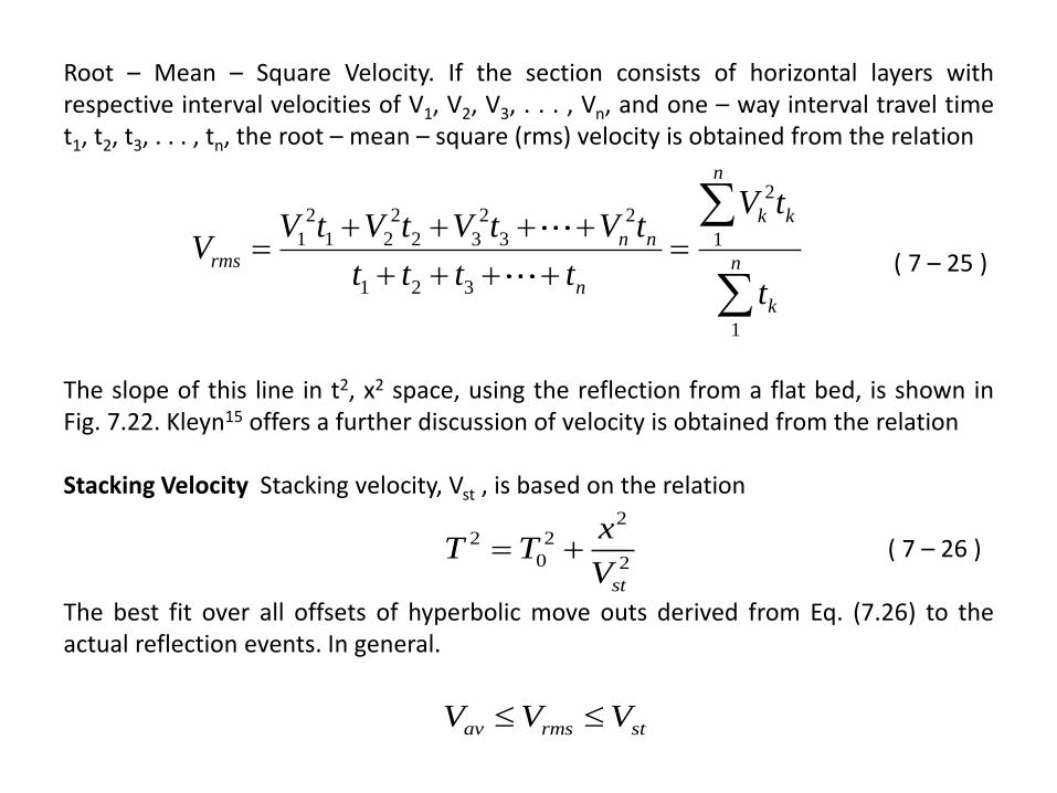
Root – Mean – Square Velocity. If the section consists of horizontal layers withrespective interval velocities of V1, V2, V3, . . . , Vn, and one – way interval travel timet1, t2, t3, . . . , tn, the root – mean – square (rms) velocity is obtained from the relation
( 7 – 25 )
The slope of this line in t2, x2 space, using the reflection from a flat bed, is shown inFig. 7.22. Kleyn15 offers a further discussion of velocity is obtained from the relation
Stacking Velocity Stacking velocity, Vst , is based on the relation
( 7 – 26 )
The best fit over all offsets of hyperbolic move outs derived from Eq. (7.26) to theactual reflection events. In general.
2
2 2 2 2
1 1 2 2 3 3 1
1 2 3
1
n
k k
n nrms n
nk
V tV t V t V t V t
Vt t t t
t
22 2
0 2
st
av rms st
xT T
V
V V V
Mirror or fold plane, so that
the times ( T, T0) are two
way time.
T
½T½T½T0
½T0 ½T
T0
X
Offset
Source Reseive
r
2
2 2
0
XT T
V
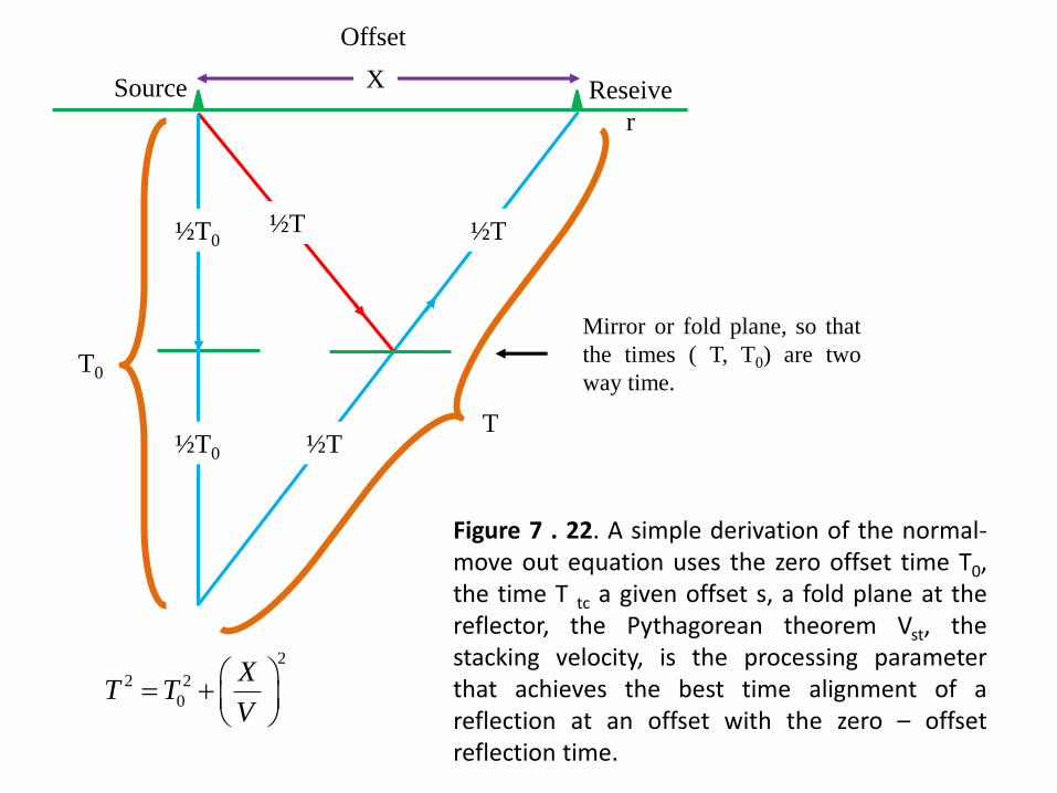
Figure 7 . 22. A simple derivation of the normal-move out equation uses the zero offset time T0,the time T tc a given offset s, a fold plane at thereflector, the Pythagorean theorem Vst, thestacking velocity, is the processing parameterthat achieves the best time alignment of areflection at an offset with the zero – offsetreflection time.
x
Sd
Shot ZQ
D
Well
Detector
1
cos SD
Z d
T
Recording Truck
16000
14000
12000
10000
8000
6000
4000
2000
20001000 3000 4000 5000 6000 7000
Depth ft
Vel
oci
ty f
t/se
c
Interval Velocity
Average overall velocity, V̅
Detector positions
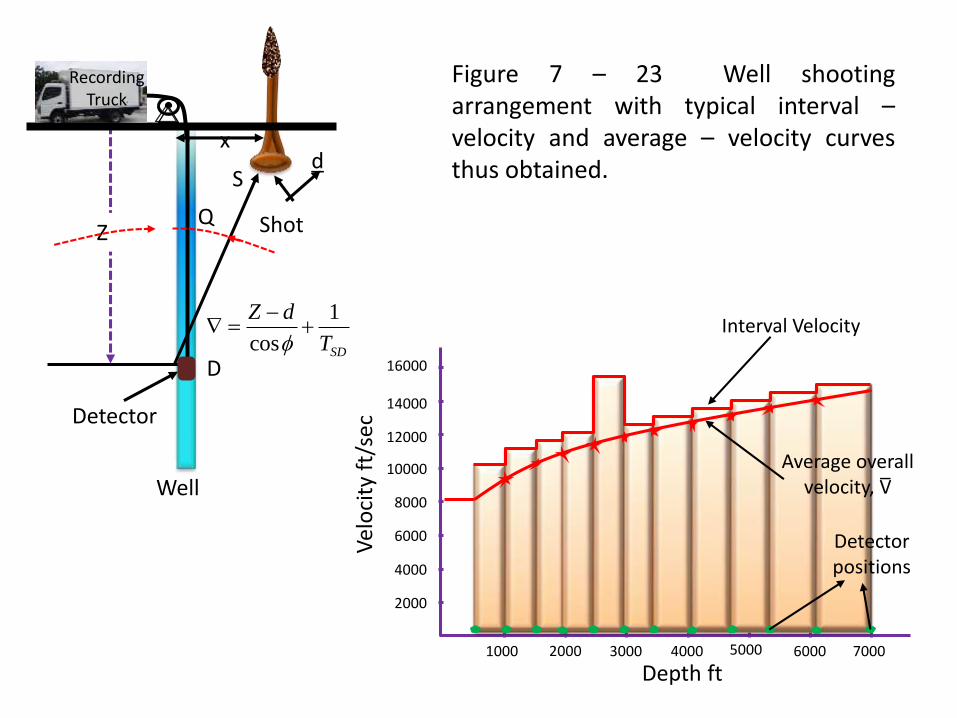
Figure 7 – 23 Well shootingarrangement with typical interval –velocity and average – velocity curvesthus obtained.
t
A B
Z True locations of reflecting
points
True locations of reflecting
points
Apparent reflecting points positions
when plotted vertically below
reflection spreads
(a) (b)
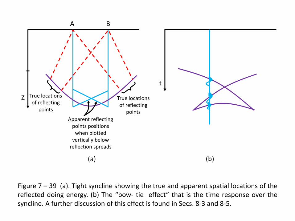
Figure 7 – 39 (a). Tight syncline showing the true and apparent spatial locations of thereflected doing energy. (b) The “bow- tie effect” that is the time response over thesyncline. A further discussion of this effect is found in Secs. 8-3 and 8-5.
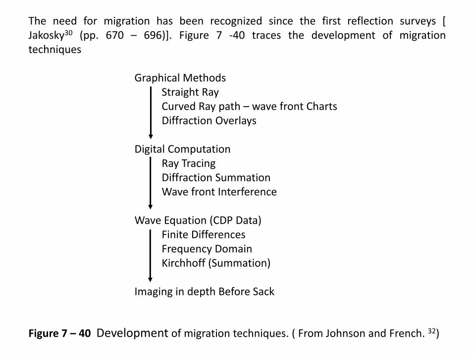
The need for migration has been recognized since the first reflection surveys [Jakosky30 (pp. 670 – 696)]. Figure 7 -40 traces the development of migrationtechniques
Graphical MethodsStraight Ray Curved Ray path – wave front ChartsDiffraction Overlays
Digital Computation Ray Tracing Diffraction Summation Wave front Interference
Wave Equation (CDP Data)Finite Differences Frequency Domain Kirchhoff (Summation)
Imaging in depth Before Sack
Figure 7 – 40 Development of migration techniques. ( From Johnson and French. 32)
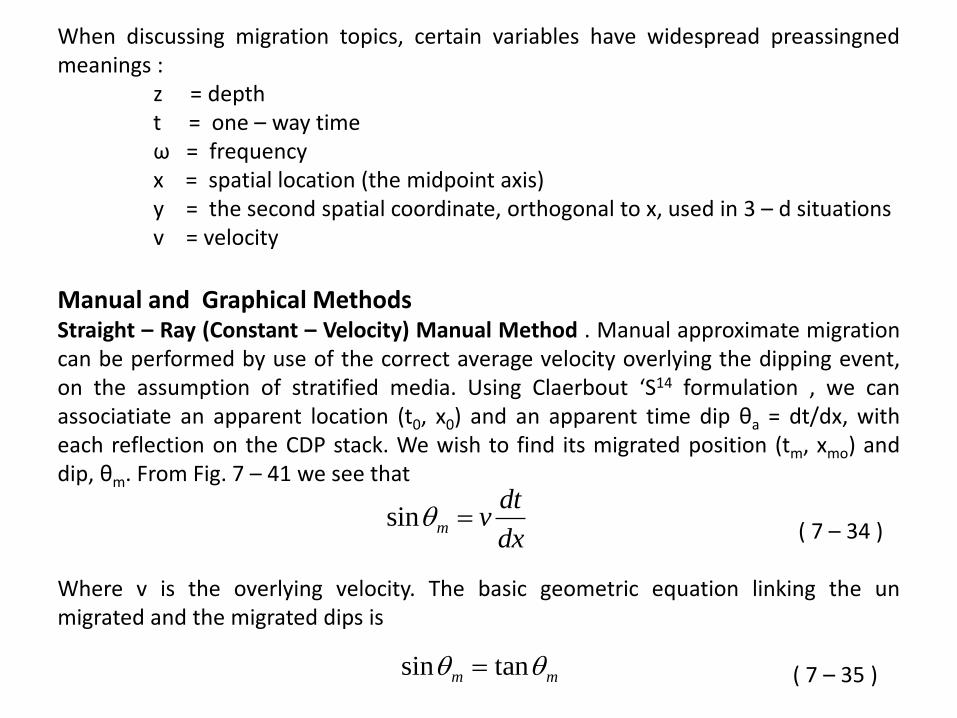
When discussing migration topics, certain variables have widespread preassingnedmeanings :
z = deptht = one – way timeω = frequencyx = spatial location (the midpoint axis)y = the second spatial coordinate, orthogonal to x, used in 3 – d situationsv = velocity
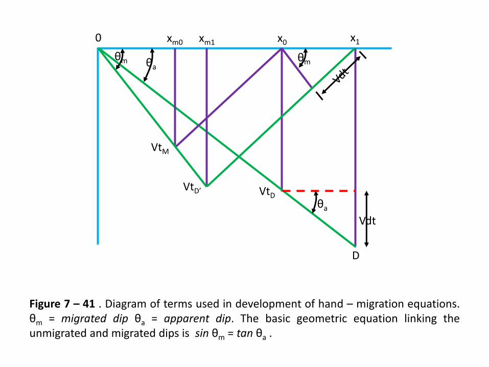
Manual and Graphical MethodsStraight – Ray (Constant – Velocity) Manual Method . Manual approximate migrationcan be performed by use of the correct average velocity overlying the dipping event,on the assumption of stratified media. Using Claerbout ‘S14 formulation , we canassociatiate an apparent location (t0, x0) and an apparent time dip θa = dt/dx, witheach reflection on the CDP stack. We wish to find its migrated position (tm, xmo) anddip, θm. From Fig. 7 – 41 we see that
( 7 – 34 )
Where v is the overlying velocity. The basic geometric equation linking the unmigrated and the migrated dips is
( 7 – 35 )
sin m
dtv
dx
sin tanm m
0 xm0 xm1 x0 x1
θmθaθm
θa
VtM
VtD’ VtD
D
Vdt
Figure 7 – 41 . Diagram of terms used in development of hand – migration equations.θm = migrated dip θa = apparent dip. The basic geometric equation linking theunmigrated and migrated dips is sin θm = tan θa .
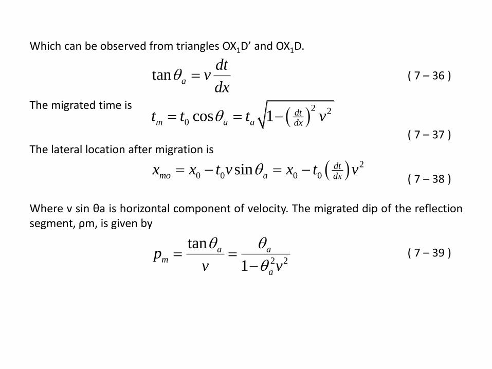
Which can be observed from triangles OX1D’ and OX1D.
( 7 – 36 )
The migrated time is
( 7 – 37 )The lateral location after migration is
( 7 – 38 )
Where v sin θa is horizontal component of velocity. The migrated dip of the reflectionsegment, ρm, is given by
( 7 – 39 )
2 2
0
2
0 0 0 0
2 2
tan
cos 1
sin
tan
1
a
dtm a a dx
dtmo a dx
a am
a
dtv
dx
t t t v
x x t v x t v
pv v
0
1
2
3
4-4 -2 2 4 km sec
( a )
-4 -2 2 4 km0
0
1
2
3
4sec
0
( b )
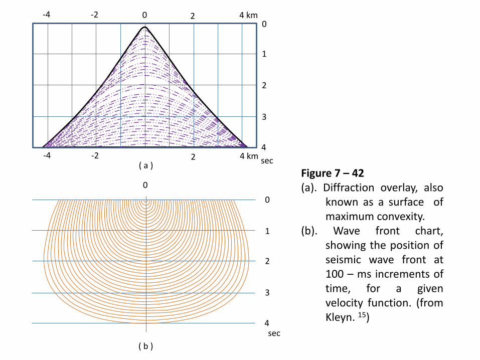
Figure 7 – 42(a). Diffraction overlay, also
known as a surface ofmaximum convexity.
(b). Wave front chart,showing the position ofseismic wave front at100 – ms increments oftime, for a givenvelocity function. (fromKleyn. 15)
S1 S2
R2
R1
R’2
R’1
D
X
T
MAC curve
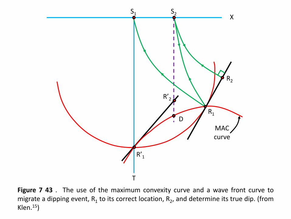
Figure 7 43 . The use of the maximum convexity curve and a wave front curve tomigrate a dipping event, R1 to its correct location, R2, and determine its true dip. (fromKlen.15)
Top Related