


Languages
Pages
Legal

General Mission Analysis Tool (GMAT)
User Guide
The GMAT Development Team
18 May 2012

General Mission Analysis Tool (GMAT): User Guide
General Mission Analysis Tool(GMAT)
iii
Table of ContentsPreface ............................................................................................................................ viI. Introduction .................................................................................................................. 1
Introduction to GMAT ............................................................................................. 2Licensing .......................................................................................................... 2Platform Support .............................................................................................. 2User Interfaces ................................................................................................. 3Development Status .......................................................................................... 3Contributors ..................................................................................................... 3
Getting Started ......................................................................................................... 4Installation ....................................................................................................... 4Starting and Quitting GMAT ............................................................................. 4Running the GMAT Demos .............................................................................. 4User Interfaces Overview .................................................................................. 5Data and Configuration ................................................................................... 10Other Resources ............................................................................................. 16
II. Creating Your First Mission ......................................................................................... 17Simulating an Orbit ................................................................................................. 18
Objective and Overview .................................................................................. 18Configure the Spacecraft .................................................................................. 18Configure the Propagator ................................................................................. 20Configure the Propagate Command .................................................................. 21Run and Analyze the Results ............................................................................ 22
III. Common Tasks ......................................................................................................... 24Configuring a Spacecraft .......................................................................................... 25
Setting the Initial Epoch .................................................................................. 25Configuring the Orbit ...................................................................................... 25Configuring Physical Properties ........................................................................ 26Configuring the Attitude (Fixed) ....................................................................... 27Configuring the Attitude (Spinner) .................................................................... 27
Propagating a Spacecraft .......................................................................................... 29Configuring the Force Model ........................................................................... 29Configuring the Force Model: Mars .................................................................. 29Propagating for a Duration .............................................................................. 30Propagating to an Orbit Condition ................................................................... 31
Reporting Data ....................................................................................................... 32Reporting Data During a Propagation Span ....................................................... 32Reporting Data at a Specific Mission Event ....................................................... 32Creating a CCSDS Ephemeris File .................................................................... 33Creating an SPK Ephemeris File ...................................................................... 33
Visualizing Data ...................................................................................................... 35Manipulating the 3D Orbit View ...................................................................... 35Configuring the Ground Track Plot .................................................................. 35Creating a 2D Plot .......................................................................................... 35
IV. Tutorials ................................................................................................................... 37Simple Orbit Transfer .............................................................................................. 38
Objective and Overview .................................................................................. 38
General Mission Analysis Tool(GMAT)
iv
Configure Maneuvers, Differential Corrector, and Graphics ................................. 38Configure the Mission Sequence ....................................................................... 39Run the Mission ............................................................................................. 46
V. Reference Guide ......................................................................................................... 48I. Resources ............................................................................................................ 50
Array ............................................................................................................. 51Barycenter ...................................................................................................... 52CelestialBodies ................................................................................................ 53CoordinateSystem ............................................................................................ 57DifferentialCorrector ....................................................................................... 58EphemerisFile ................................................................................................. 61EphemerisPropagator ...................................................................................... 62FiniteBurn ...................................................................................................... 63Formation ...................................................................................................... 65FuelTank ........................................................................................................ 66GMATFunction .............................................................................................. 69GroundStation ................................................................................................ 70GroundTrackPlot ............................................................................................ 71ImpulsiveBurn ................................................................................................ 74LibrationPoint ................................................................................................. 76MATLABFunction .......................................................................................... 78OrbitView ...................................................................................................... 79Propagator ...................................................................................................... 85ReportFile ...................................................................................................... 92SolarSystem .................................................................................................... 95Spacecraft ....................................................................................................... 97SQP ............................................................................................................. 106String ........................................................................................................... 109Thruster ....................................................................................................... 110Variable ........................................................................................................ 115VF13adOptimizer .......................................................................................... 116XYPlot ......................................................................................................... 117
II. Commands ....................................................................................................... 119Achieve ........................................................................................................ 120BeginFiniteBurn ............................................................................................ 121BeginMissionSequence ................................................................................... 122CallGmatFunction ......................................................................................... 123CallMatlabFunction ........................................................................................ 125ClearPlot ...................................................................................................... 126Else .............................................................................................................. 127EndFiniteBurn .............................................................................................. 128Equation ....................................................................................................... 129For ............................................................................................................... 130Global .......................................................................................................... 133If ................................................................................................................. 134Maneuver ...................................................................................................... 136MarkPoint ..................................................................................................... 137Minimize ...................................................................................................... 138NonlinearConstraint ....................................................................................... 139
General Mission Analysis Tool(GMAT)
v
Optimize ...................................................................................................... 141PenUp .......................................................................................................... 142PenDown ..................................................................................................... 143Propagate ..................................................................................................... 144Report .......................................................................................................... 147Save ............................................................................................................. 148SaveMission .................................................................................................. 149ScriptEvent ................................................................................................... 150Stop ............................................................................................................. 151Target ........................................................................................................... 152Toggle .......................................................................................................... 156Vary ............................................................................................................. 157While ........................................................................................................... 160
VI. Release Notes .......................................................................................................... 162GMAT R2011a Release Notes ................................................................................ 163
New Features ................................................................................................ 163Improvements ............................................................................................... 166Compatibility Changes ................................................................................... 168Fixed Issues .................................................................................................. 170Known Issues ............................................................................................... 170
GMAT R2012a Release Notes ................................................................................ 174New Features ................................................................................................ 174Improvements ............................................................................................... 176Compatibility Changes ................................................................................... 179Known & Fixed Issues .................................................................................. 180
Index ........................................................................................................................... 181
Preface
vi
PrefaceThe GMAT User’s Guide contains material for new and experienced users and is organized intothe following sections:
• Introduction• Creating Your First Mission• Common Tasks• Tutorials• Reference Guide
Introduction
The Introduction section contains two major parts: Introduction to GMAT and Getting Started.
The Introduction to GMAT section contains a brief project and software overview and discusses projectstatus, licensing, and contributors.
The Getting Started section describes how to install and start GMAT, presents an overview of the userinterfaces, and provides information on configuring your system.
Note
We consider the User Interfaces Overview essential reading. If you read nothing else,at least read this section as it will explain the basic philosophy and rules of GMAT’suser interfaces.
Creating Your First Mission
The Creating Your First Mission section walks you step-by-step through a sample mission, includ-ing creating a spacecraft, a propagator, and an OrbitView graphical display, and propagating thespacecraft to orbit perigee.
Common Tasks
The Common Tasks section contains many short articles that each describe a single area of func-tionality. The purpose of the how-to documentation is to show you how to use a specific featurein an analysis context, and these articles often start from the default mission that is loaded whenyou start GMAT. A common task section is designed to take about five minutes to teach you howto perform a specific task.
Tutorials
The Tutorials section describes how to use GMAT for end-to-end analysis. Tutorials are designedto teach you how to use GMAT in the context of performing real-world analysis and are intendedto take between 30 minutes and several hours to complete. Each tutorial has a difficulty level and anapproximate duration listed with any prerequisites in its introduction.
Preface
vii
Reference Guide
The Reference Guide contains individual topics that describe each of GMAT's resources and com-mands in detail, including its syntax, options, variable ranges and data types, defaults, and expectedbehavior.
Typographical Conventions
This document uses two typographical conventions throughout:
• Graphical user interface (GUI) elements are presented in bold.• Filenames, resource and command names, and script examples are presented in monospace.
Part I. Introduction
Table of ContentsIntroduction to GMAT ..................................................................................................................... 2
Licensing .................................................................................................................................. 2Platform Support ...................................................................................................................... 2User Interfaces ......................................................................................................................... 3Development Status .................................................................................................................. 3Contributors ............................................................................................................................. 3
Getting Started ................................................................................................................................. 4Installation ............................................................................................................................... 4Starting and Quitting GMAT ..................................................................................................... 4Running the GMAT Demos ...................................................................................................... 4User Interfaces Overview .......................................................................................................... 5Data and Configuration ........................................................................................................... 10Other Resources ..................................................................................................................... 16
Introduction Introduction to GMAT
2
Introduction to GMATGMAT is an open source trajectory design and optimization system developed by NASA and privateindustry. It is developed in an open source process to maximize technology transfer, to permit anyoneto develop and validate new algorithms, and to enable those new algorithms to quickly transitioninto the high fidelity core.
GMAT is designed to model and optimize spacecraft trajectories in flight regimes ranging from lowEarth orbit to lunar, interplanetary, and other deep space missions. The system supports constrainedand unconstrained trajectory optimization and built-in features make defining cost and constraintfunctions trivial. GMAT also contains initial value solvers (propagators) and boundary value solversand efficiently propagates spacecraft either singly or as coupled sets. GMAT’s propagators naturallysynchronize the epochs of multiple vehicles and avoid fixed step integration and interpolation whendoing so.
Users can interact with GMAT using either a graphical user interface (GUI) or a custom scriptinglanguage modeled after the syntax used in The MathWorks’ MATLAB® system. All of the systemelements can be expressed through either interface, and users can convert between the two in eitherdirection.
Analysts model space missions in GMAT by first creating and configuring resources such as space-craft, propagators, optimizers, and data files. These resources are then used in a mission sequenceto model the trajectory of the spacecraft and simulate mission events. The mission sequence sup-ports commands such as nonlinear constraints, minimization, propagatation, GMAT and MATLABfunctions, inline equations, and script events.
GMAT can display trajectories in a realistic three-dimensional view, plot parameters against one an-other, and save parameters to files for later processing. The graphics capabilities are fully interactive,plotting data as a mission is run and allowing users to zoom into regions of interest. Trajectories anddata can be viewed in any coordinate system defined in GMAT, and GMAT allows users to rotatethe view and set the focus to any object in the display. The trajectory view can be animated so userscan watch the evolution of the trajectory over time.
Licensing
GMAT is licensed under the NASA Open Source Agreement v1.3. The license text is contained inthe file License.txt in root directory of the GMAT distribution.
Platform Support
GMAT is cross-platform software and runs on Windows, Linux, and Macintosh platforms, on both32-bit and 64-bit architectures. It uses the wxWidgets cross-platform user interface toolkit and canbe built using either Microsoft Visual Studio or the GNU Compiler Collection (GCC). GMAT iswritten in ANSI standard C++ (approximately 380,000 non-comment source lines of code) usingan object-oriented methodology, with a rich class structure designed to make new features simpleto incorporate.
Introduction Introduction to GMAT
3
User Interfaces
GMAT has several user interfaces. The interactive graphical user interface is introduced in moredetail in later sections. The script interface is textual and also allows the user to configure and executeall aspects of GMAT. There is a secondary MATLAB interface that allows for running the systemvia calls from MATLAB to GMAT and allows GMAT to call MATLAB functions from within theGMAT command sequence. A low-level C API is also currently under development.
Development Status
While GMAT has undergone extensive testing and is mature software, at the present time we con-sider the software to be in beta form on Windows and alpha on Linux and Mac. GMAT is not yetsufficiently verified to be used as a primary operational analysis system. It has been used to optimizemaneuvers for flight projects such as NASA’s LCROSS and ARTEMIS missions, and the Lunar Re-connaissance Orbiter, and for optimization and analysis for the OSIRIS-REx and MMS missions.However, for flight planning, we independently verify solutions generated in GMAT in the primaryoperational system.
The GMAT team is currently working on several activities including maintenance, bug fixes, andtesting, along with selected new functionality.
Contributors
The Navigation and Mission Design Branch at NASA’s Goddard Space Flight Center performsproject management activities and is involved in most phases of the development process includingrequirements, algorithms, design, and testing. The Ground Software Systems Branch performs de-sign, implementation, and integration testing. The Flight Software Branch contributes to design andimplementation. GMAT contributors include volunteers and those paid for services they provide.We welcome new contributors to the project, either as users providing feedback about the features ofthe system, or as developers interested in contributing to the implementation of the system. Currentand past contributors include:
• Thinking Systems, Inc. (system architecture and all aspects of development)• Air Force Research Lab (all aspects of development)• a.i. solutions (testing)• Boeing (algorithms and testing)• The Schafer Corporation (all aspects of development)• Honeywell Technology Solutions (testing)• Computer Sciences Corporation (requirements)
The NASA Jet Propulsion Laboratory (JPL) has provided funding for integration of the SPICEtoolkit into GMAT. Additionally, the European Space Agency’s (ESA) Advanced Concepts teamhas developed optimizer plug-ins for the Non-Linear Programming (NLP) solvers SNOPT (SparseNonlinear OPTimizer) and IPOPT (Interior Point OPTimizer).
Introduction Getting Started
4
Getting StartedInstallation
Installers and files for Windows are located on the GMAT SourceForge page at https://sourceforge.net/projects/gmat. As of this writing the latest version is R2012a, releasedMay 23, 2012.
The GMAT Windows distribution contains an installer that will install and configure GMAT for youautomatically. By default GMAT will be installed into the application data folder in your user profile,and a shortcut will be placed in the Start menu.
GMAT is available as a source code bundle for other platforms. See the GMAT Wiki for compilinginstructions.
Starting and Quitting GMAT
Starting a GMAT Session
On Microsoft Windows platforms there are several ways to start a GMAT session. If you used theGMAT installer, you can click the GMAT R2012a item in the Start menu. If you installed GMATfrom a zip file or by compiling the system, locate the bin directory in the GMAT root directoryand double-click GMAT.exe.
On the Mac, use Finder to open the bin folder located in the GMAT root directory and open theGMAT application. Alternatively, open a Terminal window, change to your installation directory, thentype the command open GMAT.app. Once GMAT is open, you can set it to remain in the dockby clicking its dock icon, then Options, then Keep in Dock. This allows you to open GMAT inthe future simply by clicking its dock icon.
Quitting a GMAT Session
To end a GMAT session on Windows or Linux, in the menu bar, click File, then click Exit. On theMac, in the menu bar, click GMAT, then click Quit GMAT, or type Command+Q.
Running the GMAT Demos
The GMAT distribution includes more than 30 sample missions. These samples show how to applyGMAT to problems ranging from the Hohmann transfer to libration point station-keeping to tra-jectory optimization. To locate and run a sample mission:
1. Open GMAT.2. On the toolbar click Open.3. Navigate to the samples folder located in the GMAT root directory.4. Double-click a script file of your choice.5. Click Run.
To run optimization missions, you will need MATLAB and the MATLAB Optimization Toolboxand/or the VF13ad plugin based on software in the Harwell Subroutine Library. These are propri-etary libraries and are not distributed with GMAT. MATLAB connectivity is not yet fully supported
Introduction Getting Started
5
in the Mac and Linux GMAT releases, and therefore you cannot run optimization missions that useMATLAB’s fmincon optimizer on those platforms.
User Interfaces Overview
GMAT offers multiple ways to design and execute your mission. The two primary interfaces are thegraphical user interface (GUI) and the script interface. These interfaces are interchangeable and eachsupports most of the functionality available in GMAT. When you work in the script interface, youare working in GMAT’s custom script language. To avoid issues such as circular dependencies, thereare some basic rules you must follow. Below, we discuss these interfaces and then discuss the basicrules and best practices for working in each interface.
GUI Overview
When you start a session, the GMAT desktop is displayed with a default mission already loaded.The GMAT desktop has a native look and feel on each platform and most desktop components aresupported on all platforms.
Windows GUI
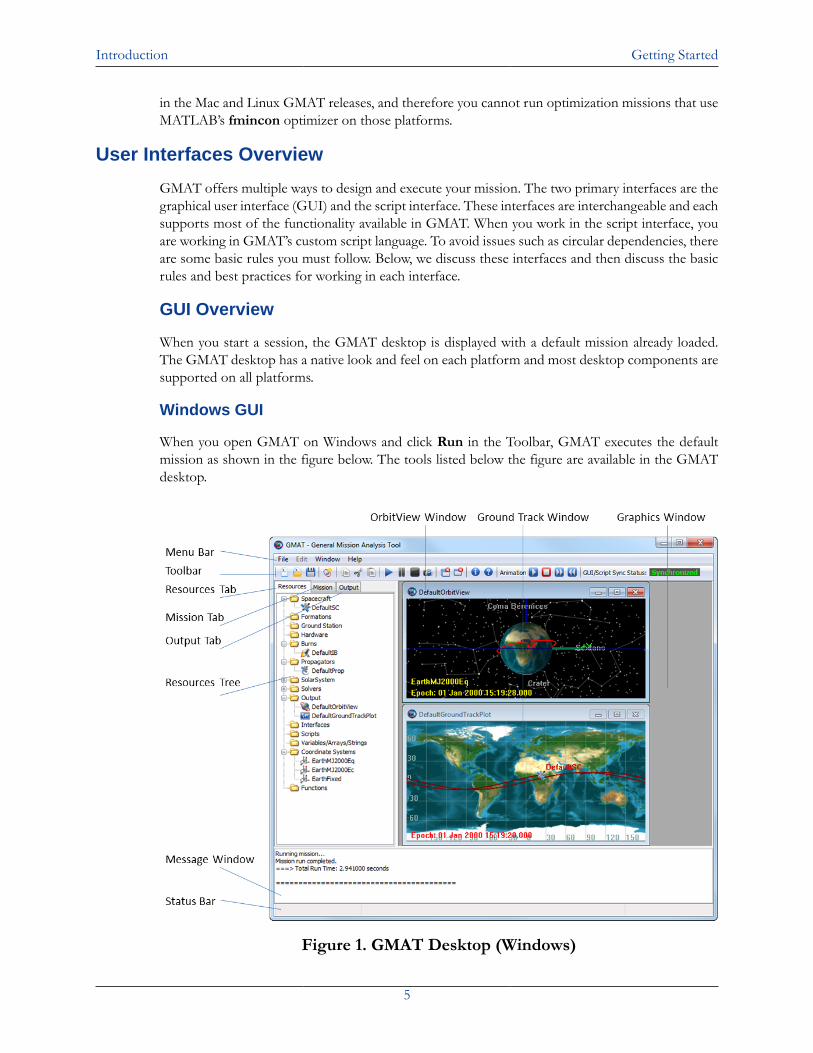
When you open GMAT on Windows and click Run in the Toolbar, GMAT executes the defaultmission as shown in the figure below. The tools listed below the figure are available in the GMATdesktop.
Figure 1. GMAT Desktop (Windows)
Introduction Getting Started
6
Menu Bar The menu bar contains File, Edit, Window and Help functionality.
On Windows, the File menu contains standard Open, Save, Save As, andExit functionality as well as Open Recent and New Mission. The Editmenu contains functionality for script editing when the script editor is active.The Window menu contains tools for organizing graphics windows andthe script editor within the GMAT desktop. Examples include the abilityto Tile windows, Cascade windows and Close windows. The Help menucontains links to Online Help, Tutorials, Forums, and the Report AnIssue option links to GMAT’s defect reporting system, the Welcome Page,and a Provide Feedback link.
On the Mac, menus are nearly the same, with a few differences: the Filemenu does not contain an Exit option - instead, the Quit GMAT menuoption is on the GMAT menu, as discussed before; tiling and cascading win-dows are not supported, so those options do not appear under the Windowmenu; currently, email is not supported, so Provide Feedback is nonfunc-tional under the Help menu.
Toolbar The toolbar provides easy access to frequently used controls such as filecontrols, Run, Pause, and Stop for mission execution, and controls forgraphics animation. On Windows and Linux, the toolbar is located at thetop of the GMAT window; on the Mac, it is located on the left of the GMATframe. Because the toolbar is vertical on the Mac, some toolbar options areabbreviated.
GMAT allows you to simultaneously edit the raw script file representationof your mission and the GUI representation of your mission. It is possibleto make inconsistent changes in these mission representations. The GUI/Script Sync Status indicator located in the toolbar shows you the stateof the two mission representations. See the the section called “GUI/ScriptInteractions and Synchronization” section for further discussion.
Resources Tab The Resources tab brings the Resources tree to the foreground of thedesktop.
Resources Tree The Resources tree displays all configured GMAT resources and organizesthem into logical groups. All objects created in a GMAT script using a Cre-ate command are found in the Resources tree in the GMAT desktop.
Mission Tab The Mission tab brings the Mission Tree to the foreground of the desktop.Mission Tree The Mission tree displays GMAT commands that control the time-ordered
sequence of events in a mission. The Mission tree contains all script linesthat occur after the BeginMissionSequence command in a GMAT script.You can undock the Mission tree as shown in the figure below by right-clicking on the Mission tab and dragging it into the graphics window. Youcan also follow these steps:1. Click on the Mission tab to bring the Mission Tree to the foreground.2. Right-click on the Mission Sequence folder in the Mission tree and
select Undock Mission Tree in the menu.
Introduction Getting Started
7
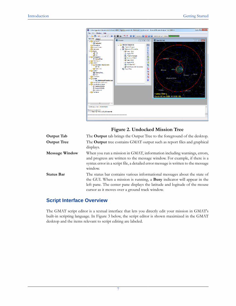
Figure 2. Undocked Mission TreeOutput Tab The Output tab brings the Output Tree to the foreground of the desktop.Output Tree The Output tree contains GMAT output such as report files and graphical
displays.Message Window When you run a mission in GMAT, information including warnings, errors,
and progress are written to the message window. For example, if there is asyntax error in a script file, a detailed error message is written to the messagewindow.
Status Bar The status bar contains various informational messages about the state ofthe GUI. When a mission is running, a Busy indicator will appear in theleft pane. The center pane displays the latitude and logitude of the mousecursor as it moves over a ground track window.
Script Interface Overview
The GMAT script editor is a textual interface that lets you directly edit your mission in GMAT'sbuilt-in scripting language. In Figure 3 below, the script editor is shown maximized in the GMATdesktop and the items relevant to script editing are labeled.
Introduction Getting Started
8
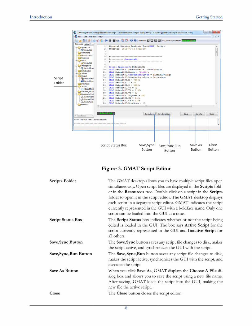
Figure 3. GMAT Script Editor
Scripts Folder The GMAT desktop allows you to have multiple script files opensimultaneously. Open script files are displayed in the Scripts fold-er in the Resources tree. Double click on a script in the Scriptsfolder to open it in the script editor. The GMAT desktop displayseach script in a separate script editor. GMAT indicates the scriptcurrently represented in the GUI with a boldface name. Only onescript can be loaded into the GUI at a time.
Script Status Box The Script Status box indicates whether or not the script beingedited is loaded in the GUI. The box says Active Script for thescript currently represented in the GUI and Inactive Script forall others.
Save,Sync Button The Save,Sync button saves any script file changes to disk, makesthe script active, and synchronizes the GUI with the script.
Save,Sync,Run Button The Save,Sync,Run button saves any script file changes to disk,makes the script active, synchronizes the GUI with the script, andexecutes the script.
Save As Button When you click Save As, GMAT displays the Choose A File di-alog box and allows you to save the script using a new file name.After saving, GMAT loads the script into the GUI, making thenew file the active script.
Close The Close button closes the script editor.
Introduction Getting Started
9
GUI/Script Interface Interactions and Rules
The GMAT desktop supports both a script interface and a GUI interface and these interfaces aredesigned to be consistent with each other. You can think of the script and GUI as different "views"of the same data: the resources and the mission command sequence. GMAT allows you to switchbetween views (script and GUI) and have the same view open in an editable state simultaneously.Below we describe the behavior, interactions, and rules of the script and GUI interfaces so you canavoid confusion and potential loss of data.
GUI/Script Interactions and Synchronization
GMAT allows you to simultaneously edit both the script file representation and the GUI representa-tion of your mission. It is possible to make inconsistent changes in these representations. The GUI/Script Sync Status window located in the toolbar indicates the state of the two representations. Onthe Mac, the status is indicated in abbreviated form in the left-hand toolbar. Synchronized (green)indicates that the script and GUI contain the same information. GUI Modified (yellow) indicatesthat there are changes in the GUI that have not been saved to the script. Script Modified (yellow)indicates that there are changes in the script that have not been loaded into the GUI. Unsynchro-nized (red) indicates that there are changes in both the script and the GUI.
Caution
GMAT will not attempt to merge or resolve simultaneous changes in the Script andGUI and you must choose which representation to save if you have made changes inboth interfaces.
The Save button in the toolbar saves the GUI representation over the script. The Save,Sync buttonon the script editor saves the script representation and loads it into the GUI.
How the GUI Maps to a Script
Clicking the Save button in the toolbar saves the GUI representation to the script file; this is the samefile you edit when working in the script editor. GUI items that appear in the Resources tree appearbefore the BeginMissionSequence command in a script file and are written in a predefined order.GUI items that appear in the Mission Tree appear after the BeginMissionSequence command ina script file in the same order as they appear in the GUI.
Caution
If you have a script file that has custom formatting such as spacing and data organiza-tion, you should work exclusively in the script. If you load your script into the GUI,then click Save in the toolbar, you will lose the formatting of your script. (You will not,however, lose the data.)
How the Script Maps to the GUI
Clicking the Save,Sync button on the script editor saves the script representation and loads it into theGUI. When you work in a GMAT script, you work in the raw file that GMAT reads and writes. Each
Introduction Getting Started
10
script file must contain a command called BeginMissionSequence. Script lines that appear beforethe BeginMissionSequence command create and configure models and this data will appear in theResources tree in the GUI. Script lines that appear after the BeginMissionSequence commanddefine your mission sequence and appear in the Mission tree in the GUI. Here is a brief scriptexample to illustrate:
Create Spacecraft SatSat.X = 3000BeginMissionSequenceSat.X = 1000
The line Sat.X = 3000 sets the x-component of the Cartesian state to 3000; this value will appearon the Orbit tab of the Spacecraft dialog box. However, because the line Sat.X = 1000 appearsafter the BeginMissionSequence command, the line Sat.X = 1000 will appear as an assignmentcommand in the Mission tree in the GUI.
Basic Script Syntax Rules
• Each script file must contain one and only one BeginMissionSequence command.• GMAT commands are not allowed before the BeginMissionSequence command.• You cannot use inline math statements (equations) before the BeginMissionSequence com-
mand in a script file. (GMAT considers in-line math statements to be an assignment command.You cannot use equations in the Resources tree, so you also cannot use equations before theBeginMissionSequence command.)
• In the GUI, you can only use in-line math statements in an assignment command. So, you cannottype 3000 + 4000 or Sat.Y - 8 in the text box for setting a spacecraft’s dry mass.
• GMAT’s script language is case-sensitive.
Data and Configuration
Below we discuss the files and data that are distributed with GMAT and are required for GMATexecution. GMAT uses many types of data files, including planetary ephemeris files, Earth orienta-tion data, leap second files, and gravity coefficient files. This section describes how these files areorganized and the controls provided to customize them.
File Structure
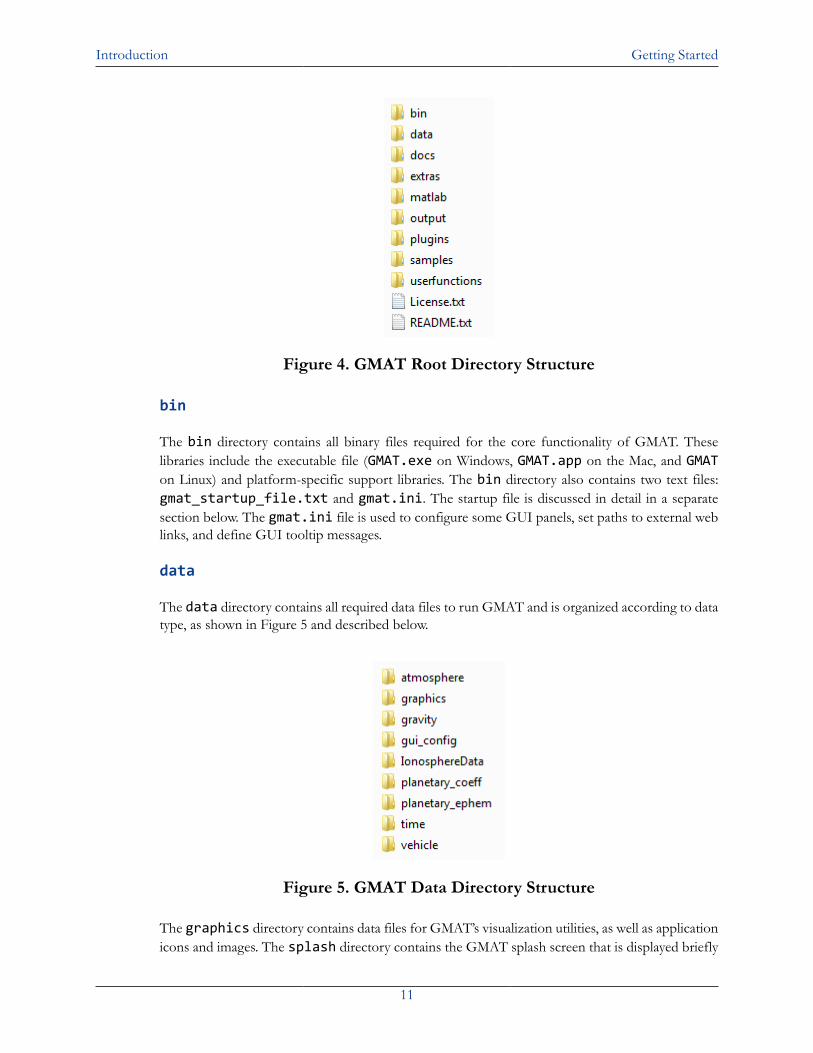
The default directory structure for GMAT is broken into eight main subdirectories, as shown inFigure 4. These directories organize the files and data used to run GMAT, including binary li-braries, data files, texture maps, and 3D models. The only two files in the GMAT root directory arelicense.txt, which contains the text of the NASA Open Source Agreement, and README.txt,which contains user information for the current GMAT release. A summary of the contents of eachsubdirectory is provided in the sections below.
Introduction Getting Started
11
Figure 4. GMAT Root Directory Structure
bin
The bin directory contains all binary files required for the core functionality of GMAT. Theselibraries include the executable file (GMAT.exe on Windows, GMAT.app on the Mac, and GMATon Linux) and platform-specific support libraries. The bin directory also contains two text files:gmat_startup_file.txt and gmat.ini. The startup file is discussed in detail in a separatesection below. The gmat.ini file is used to configure some GUI panels, set paths to external weblinks, and define GUI tooltip messages.
data
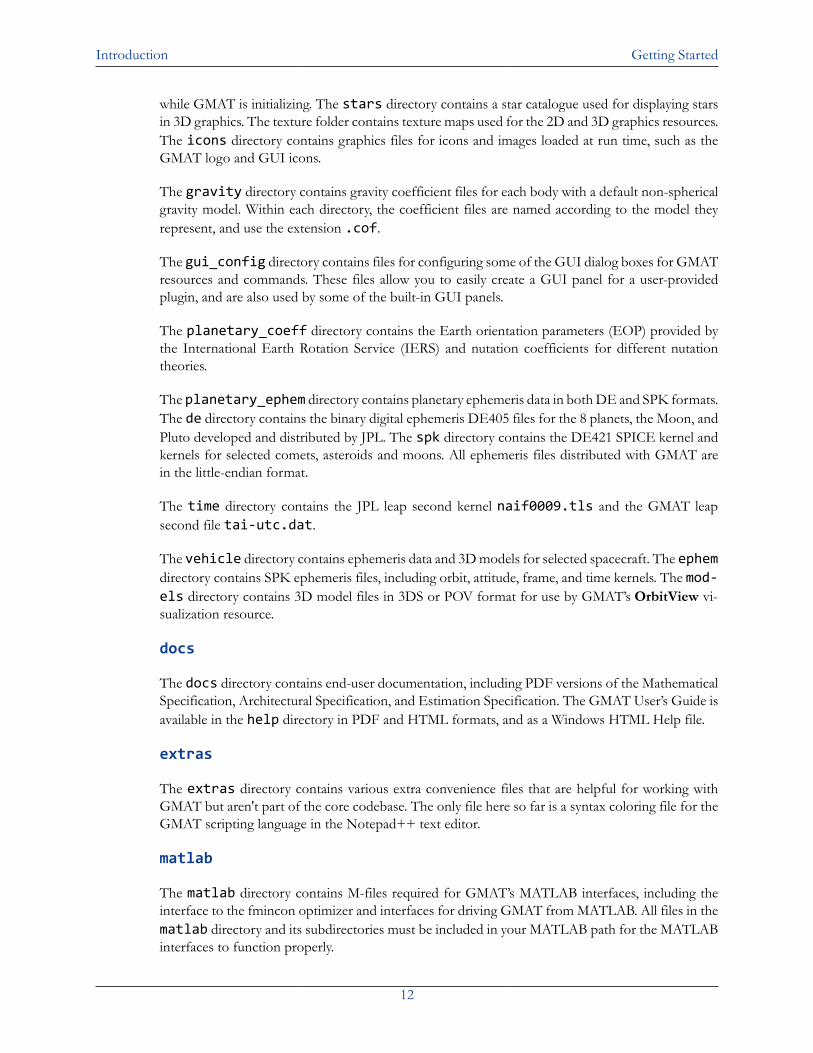
The data directory contains all required data files to run GMAT and is organized according to datatype, as shown in Figure 5 and described below.
Figure 5. GMAT Data Directory Structure
The graphics directory contains data files for GMAT’s visualization utilities, as well as applicationicons and images. The splash directory contains the GMAT splash screen that is displayed briefly
Introduction Getting Started
12
while GMAT is initializing. The stars directory contains a star catalogue used for displaying starsin 3D graphics. The texture folder contains texture maps used for the 2D and 3D graphics resources.The icons directory contains graphics files for icons and images loaded at run time, such as theGMAT logo and GUI icons.
The gravity directory contains gravity coefficient files for each body with a default non-sphericalgravity model. Within each directory, the coefficient files are named according to the model theyrepresent, and use the extension .cof.
The gui_config directory contains files for configuring some of the GUI dialog boxes for GMATresources and commands. These files allow you to easily create a GUI panel for a user-providedplugin, and are also used by some of the built-in GUI panels.
The planetary_coeff directory contains the Earth orientation parameters (EOP) provided bythe International Earth Rotation Service (IERS) and nutation coefficients for different nutationtheories.
The planetary_ephem directory contains planetary ephemeris data in both DE and SPK formats.The de directory contains the binary digital ephemeris DE405 files for the 8 planets, the Moon, andPluto developed and distributed by JPL. The spk directory contains the DE421 SPICE kernel andkernels for selected comets, asteroids and moons. All ephemeris files distributed with GMAT arein the little-endian format.
The time directory contains the JPL leap second kernel naif0009.tls and the GMAT leapsecond file tai-utc.dat.
The vehicle directory contains ephemeris data and 3D models for selected spacecraft. The ephemdirectory contains SPK ephemeris files, including orbit, attitude, frame, and time kernels. The mod-els directory contains 3D model files in 3DS or POV format for use by GMAT’s OrbitView vi-sualization resource.
docs
The docs directory contains end-user documentation, including PDF versions of the MathematicalSpecification, Architectural Specification, and Estimation Specification. The GMAT User’s Guide isavailable in the help directory in PDF and HTML formats, and as a Windows HTML Help file.
extras
The extras directory contains various extra convenience files that are helpful for working withGMAT but aren't part of the core codebase. The only file here so far is a syntax coloring file for theGMAT scripting language in the Notepad++ text editor.
matlab
The matlab directory contains M-files required for GMAT’s MATLAB interfaces, including theinterface to the fmincon optimizer and interfaces for driving GMAT from MATLAB. All files in thematlab directory and its subdirectories must be included in your MATLAB path for the MATLABinterfaces to function properly.
Introduction Getting Started
13
output
The output directory is the default location for file output such as ephemeris files and report files.If no path information is provided for reports or ephemeris files created during a GMAT session,then those files will be written to the output folder.
plugins
The plugins directory contains optional plugins that are not required for use of GMAT. Theproprietary directory is used for for third-party libraries that cannot be distributed freely and isan empty folder in the open source distribution.
samples
The samples directory contains over 30 sample missions, ranging from a Hohmann transfer tolibration point station-keeping to Mars B-plane targeting. These files are intended to demonstrateGMAT’s capabilities and to provide you with a potential starting point for building common mis-sion types for your application and flight regime. Samples with specific requirements are located insubdirectories such as NeedMatlab and NeedVF13ad.
userfunctions
The userfunctions directory contains GMAT and MATLAB functions that are included in theGMAT distribution. You can also store your own custom GMAT and MATLAB functions in thesefolders.
Configuring GMAT Data Files
You can configure the data files GMAT loads at run time by editing thegmat_startup_file.txt file located in the bin directory. The startup file contains path infor-mation for data files such as ephemeris, Earth orientation parameters and graphics files. By editingthe startup file, you can customize which files are loaded and used during a GMAT session. Belowwe describe the customization features available in the startup file. The order of lines in the startupfile does not matter.
Leap Second and EOP files
GMAT reads several files that are used for high fidelity modelling of time and coordinate systems:the leap second files and the Earth orientation parameters (EOP) provided by the IERS. The EOPfile is updated daily by the IERS. To update your local file with the latest data, simply replace thefile eopc04_08.62-now in the data/planetary_coeff directory. Updated versions of thisfile are available from the IERS.
There are two leap second files provided with GMAT in the data/time directory. Thenaif0009.tls file is used by the JPL SPICE libraries when computing ephemerides. When a newleap second is added, you can replace this file with the new file from NAIF. GMAT reads the tai-utc.dat file for all time computations requiring leap seconds that are not performed by the SPICEutilities. When a new leap second is added, you can replace this file with the new file from the USNaval Observatory. In addtion, you can modify the file if a new leap second is added by simply
Introduction Getting Started
14
duplicating the last row and updating it with the correct information for the new leap second. Forexample, if a new leapsecond were added on 01 Jul 2013, you would add the following line to thebottom of tai-utc.dat:
2013 JUL 1 =JD 2456474.5 TAI-UTC= 35.0 S + (MJD - 41317.) X 0.0
Loading Custom Plugins
Custom plugins are loaded by adding a line to the startup file (bin/gmat_startup_file.txt)specifying the name and location of the plugin file. In order for a plugin to work with GMAT, the plu-gin library must be placed in the folder referenced in the startup file. You specify the path to a pluginfile using the "PLUGIN" keyword and specify the file by providing its name without the file exten-sion (.dll on Windows). For example, to load a Windows plugin named libVF13Optimizer.dlllocated in the plugins/proprietary directory, you would add this line to your startup file:
PLUGIN = ../plugins/proprietary/libVF13Optimizer
User-defined Function Paths
If you create custom GMAT or MATLAB functions, you can provide the path to those files andGMAT will locate them at run time. The default startup file is configured so you can place GMATfunction files (with a .gmf extension) in the userfunctions/gmat directory and place MATLABfunctions (with a .m extension) in the userfunctions/matlab directory. GMAT automaticallysearches those locations at run time. You can change the location of the search path to your GMATor MATLAB functions by changing these lines in your startup file to reflect the location of yourfiles with respect to the GMAT bin folder:
GMAT_FUNCTION_PATH = ../userfunctions/gmatMATLAB_FUNCTION_PATH = ../userfunctions/matlab
If you wish to organize your custom functions in multiple folders, you can add multiple search pathsto the startup file. For example,
GMAT_FUNCTION_PATH = ../MyFunctions/utilsGMAT_FUNCTION_PATH = ../MyFunctions/StateConversion GMAT_FUNCTION_PATH = ../MyFunctions/TimeConversion
GMAT will search the paths in the order specified in the startup file and will use the first functionwith a matching name.
Configuring the MATLAB Interface
GMAT features a MATLAB interface that allows you to run MATLAB functions from withinGMAT.
This interface is packaged as an optional GMAT plugin. To use it, make sure the following line ispresent in your gmat_startup_file.txt and has no comment symbol (#) in front of it.
PLUGIN = ../plugins/libMatlabInterface
The MATLAB interface must be able to find your MATLAB installation. The procedure for settingthis information varies by platform.
Introduction Getting Started
15
Windows
On Windows, MATLAB must be properly configured in two places: the system Path variable andthe Windows registry. Both locations must be configured for the same MATLAB version.
1. The following directories must exist in your system’s Path variable, where <MATLAB> is the pathto the MATLAB root directory:
<MATLAB>/bin/win32<MATLAB>/bin
If you have multiple versions of MATLAB installed, GMAT will use the one that appears firstin the system path.
Caution
For some versions of MATLAB (e.g. R2010a), MATLAB and Windows are distrib-uted with libraries that have the same name, resulting in a conflict. As a workaround,you may need to place the folders above at the beginning of your system path.
2. When you install MATLAB, it automatically registers itself as a COM server in the Windowsregistry. If you have mulple versions of MATLAB installed, it may be necessary to re-register acertain version manually. This can be done by running the following command. This may requireadministrator privileges.
matlab.exe -regserver
3. Add GMAT’s MATLAB files to your MATLAB path. This can be done by placing the followingline in a file named startup.m in your user MATLAB directory, where <GMAT> is the path toyour GMAT root directory.
addpath(genpath('<GMAT>/matlab'));
Mac OS X
On Mac OS X, to use MATLAB with GMAT, you must set the MATLABFORGMAT environmentvariable in your environment.plist file, located in the .MacOSX directory in your home folder.This environment variable should point to the location of your MATLAB installation (applicationbundle). GMAT will not interface with MATLAB unless this environment variable is set.
The current Mac application includes the ability to make calls to MATLAB functions from withinGMAT, but does not support calls MATLAB to GMAT (including the fmincon optimizer).
Note that when GMAT opens MATLAB, it will open X11 first (as is required for MATLAB execu-tion). GMAT currently does not automatically close X11 after quitting MATLAB, so you will needto quit X11 manually.
To add the environment variable:
1. If the environment.plist file already exists in your .MacOSX directory, edit the fileusing the Property List Editor to add the MATLABFORGMAT variable and set it to point
Introduction Getting Started
16
to the location of your MATLAB application (e.g. /Applications/MATLAB_R2010a/MATLAB_R2010a.app).
2. If you do not have an environment.plist file in your .MacOSX directory, open a Terminalwindow and follow these steps:
1. Create the .MacOSX directory as a directory in your home folder (if it does not exist).2. Open the Property List Editor and create the MATLABFORGMAT variable as described
above.3. Save the property list as environment.plist in the .MacOSX directory.
You must logout and log back in for this to take effect.
Other Resources
If you have further questions, need help with using GMAT, or want to provide feedback, here aresome additional resources:
• Official Homepage: http://gmat.gsfc.nasa.gov• User Forum: http://gmat.ed-pages.com/forum• Wiki: http://gmat.ed-pages.com/wiki• Mailing Lists and Project Resources: http://sourceforge.net/projects/gmat• Blog: http://gmat.sourceforge.net/blog• Documentation: http://gmat.sourceforge.net/docs• Bug Tracker: http://pows003.gsfc.nasa.gov/bugzilla• Official Contact: <[email protected]>
Part II. Creating Your First Mission
Table of ContentsSimulating an Orbit ......................................................................................................................... 18
Objective and Overview .......................................................................................................... 18Configure the Spacecraft .......................................................................................................... 18Configure the Propagator ........................................................................................................ 20Configure the Propagate Command .......................................................................................... 21Run and Analyze the Results .................................................................................................... 22
Creating Your First Mission Simulating an Orbit
18
Simulating an OrbitAudience BeginnerLength 30 minutesPrerequisites NoneScript File Tut_SimulatingAnOrbit.script
Objective and Overview
Note
The most fundamental capability of GMAT is to propagate, or simulate the orbitalmotion of, spacecraft. The ability to propagate spacecraft is used in nearly every practicalaspect of space mission analysis, from simple orbital predictions (e.g. When will theInternational Space Station be over my house?) to complex analyses that determine thethruster firing sequence required to send a spacecraft to the Moon or Mars.
This tutorial will teach you how to use GMAT to propagate a spacecraft. You will learn how to con-figure Spacecraft and Propagator resources, and how to use the Propagate command to propa-gate the spacecraft to orbit periapsis, which is the point of minimum distance between the spacecraftand Earth. The basic steps in this tutorial are:
1. Configure a Spacecraft and define its epoch and orbital elements.2. Configure a Propagator.3. Modify the default OrbitView plot to visualize the spacecraft trajectory.4. Modify the Propagate command to propagate the spacecraft to periapsis.5. Run the mission and analyze the results.
Configure the Spacecraft
In this section, you will rename the default Spacecraft and set the Spacecraft’s initial epoch andclassical orbital elements. You’ll need GMAT open, with the default mission loaded. To load thedefault mission, click New Mission ( ) or start a new GMAT session.
Rename the Spacecraft
1. In the Resources tree, right-click DefaultSC and click Rename.2. Type Sat.3. Click OK.
Set the Spacecraft Epoch
1. In the Resources tree, double-click Sat. Click the Orbit tab if it is not already selected.2. In the Epoch Format list, select UTCGregorian. You’ll see the value in the Epoch field change
to the UTC Gregorian epoch format.3. In in the Epoch box, type 22 Jul 2014 11:29:10.811. This field is case-sensitive.4. Click Apply or press the ENTER key to save these changes.
Creating Your First Mission Simulating an Orbit
19
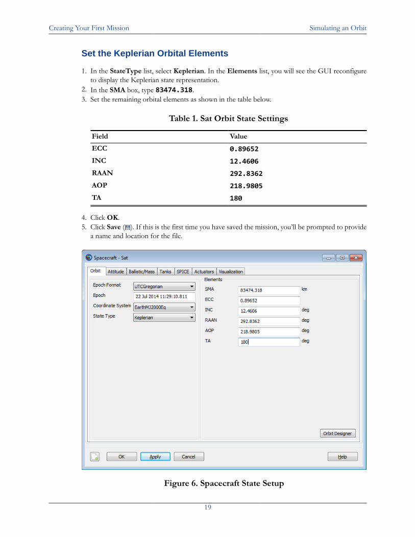
Set the Keplerian Orbital Elements
1. In the StateType list, select Keplerian. In the Elements list, you will see the GUI reconfigureto display the Keplerian state representation.
2. In the SMA box, type 83474.318.3. Set the remaining orbital elements as shown in the table below.
Table 1. Sat Orbit State Settings
Field Value
ECC 0.89652INC 12.4606RAAN 292.8362AOP 218.9805TA 180
4. Click OK.5. Click Save ( ). If this is the first time you have saved the mission, you’ll be prompted to provide
a name and location for the file.
Figure 6. Spacecraft State Setup
Creating Your First Mission Simulating an Orbit
20
Configure the Propagator
In this section you’ll rename the default Propagator and configure the force model.
Rename the Propagator
1. In the Resources tree, right-click DefaultProp and click Rename.2. Type LowEarthProp.3. Click OK.
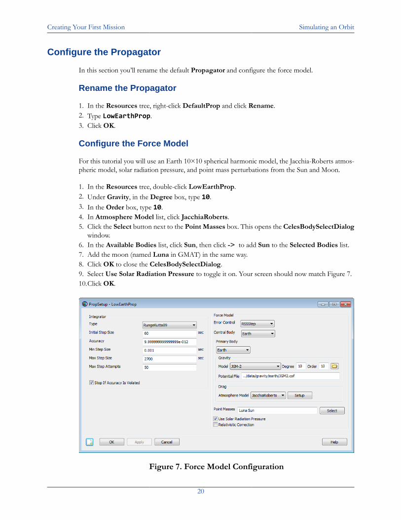
Configure the Force Model
For this tutorial you will use an Earth 10×10 spherical harmonic model, the Jacchia-Roberts atmos-pheric model, solar radiation pressure, and point mass perturbations from the Sun and Moon.
1. In the Resources tree, double-click LowEarthProp.2. Under Gravity, in the Degree box, type 10.3. In the Order box, type 10.4. In Atmosphere Model list, click JacchiaRoberts.5. Click the Select button next to the Point Masses box. This opens the CelesBodySelectDialog
window.6. In the Available Bodies list, click Sun, then click -> to add Sun to the Selected Bodies list.7. Add the moon (named Luna in GMAT) in the same way.8. Click OK to close the CelesBodySelectDialog.9. Select Use Solar Radiation Pressure to toggle it on. Your screen should now match Figure 7.10.Click OK.
Figure 7. Force Model Configuration
Creating Your First Mission Simulating an Orbit
21
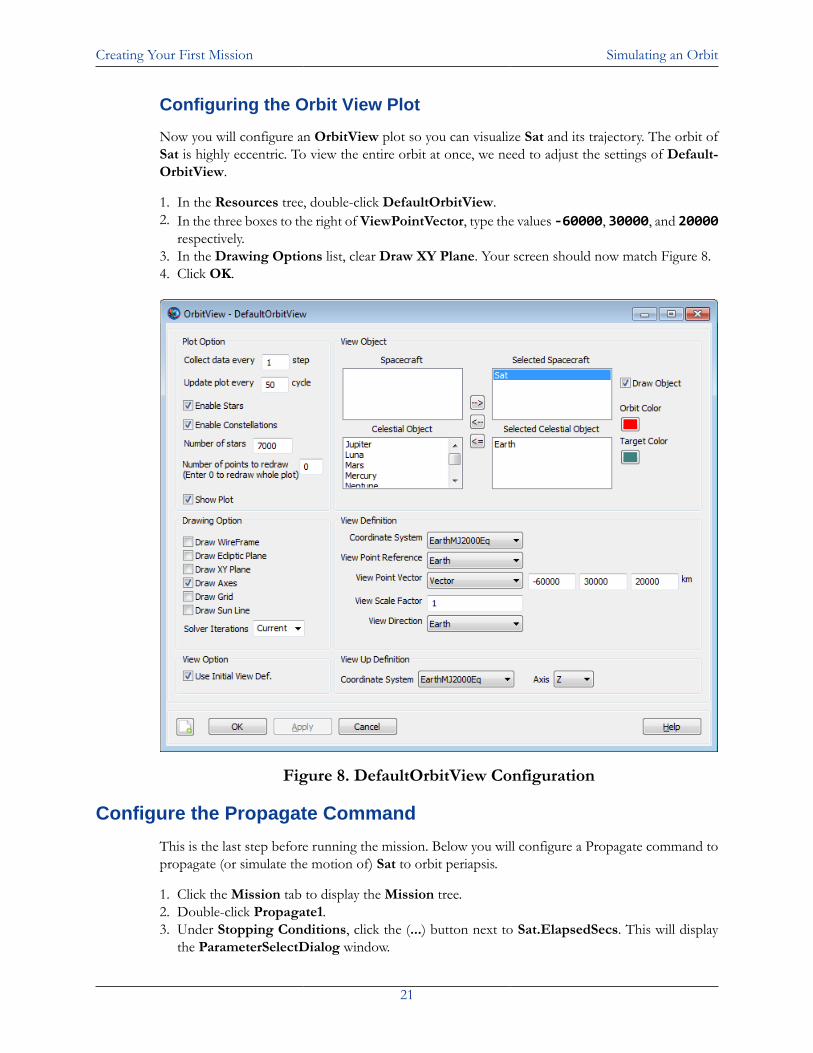
Configuring the Orbit View Plot
Now you will configure an OrbitView plot so you can visualize Sat and its trajectory. The orbit ofSat is highly eccentric. To view the entire orbit at once, we need to adjust the settings of Default-OrbitView.
1. In the Resources tree, double-click DefaultOrbitView.2. In the three boxes to the right of ViewPointVector, type the values -60000, 30000, and 20000
respectively.3. In the Drawing Options list, clear Draw XY Plane. Your screen should now match Figure 8.4. Click OK.
Figure 8. DefaultOrbitView Configuration
Configure the Propagate Command
This is the last step before running the mission. Below you will configure a Propagate command topropagate (or simulate the motion of) Sat to orbit periapsis.
1. Click the Mission tab to display the Mission tree.2. Double-click Propagate1.3. Under Stopping Conditions, click the (...) button next to Sat.ElapsedSecs. This will display
the ParameterSelectDialog window.
Creating Your First Mission Simulating an Orbit
22
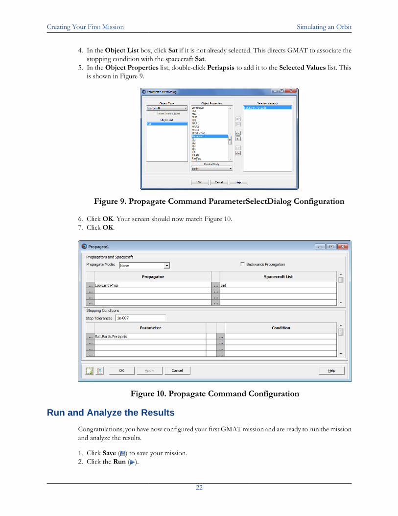
4. In the Object List box, click Sat if it is not already selected. This directs GMAT to associate thestopping condition with the spacecraft Sat.
5. In the Object Properties list, double-click Periapsis to add it to the Selected Values list. Thisis shown in Figure 9.
Figure 9. Propagate Command ParameterSelectDialog Configuration
6. Click OK. Your screen should now match Figure 10.7. Click OK.
Figure 10. Propagate Command Configuration
Run and Analyze the Results
Congratulations, you have now configured your first GMAT mission and are ready to run the missionand analyze the results.
1. Click Save ( ) to save your mission.2. Click the Run ( ).
Creating Your First Mission Simulating an Orbit
23
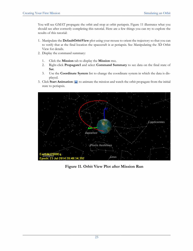
You will see GMAT propagate the orbit and stop at orbit periapsis. Figure 11 illustrates what youshould see after correctly completing this tutorial. Here are a few things you can try to explore theresults of this tutorial:
1. Manipulate the DefaultOrbitView plot using your mouse to orient the trajectory so that you canto verify that at the final location the spacecraft is at periapsis. See Manipulating the 3D OrbitView for details.
2. Display the command summary:
1. Click the Mission tab to display the Mission tree.2. Right-click Propagate1 and select Command Summary to see data on the final state of
Sat.3. Use the Coordinate System list to change the coordinate system in which the data is dis-
played.3. Click Start Animation ( ) to animate the mission and watch the orbit propagate from the initial
state to periapsis.
Figure 11. Orbit View Plot after Mission Run
Part III. Common Tasks
Table of ContentsConfiguring a Spacecraft .................................................................................................................. 25
Setting the Initial Epoch .......................................................................................................... 25Configuring the Orbit .............................................................................................................. 25Configuring Physical Properties ................................................................................................ 26Configuring the Attitude (Fixed) ............................................................................................... 27Configuring the Attitude (Spinner) ............................................................................................ 27
Propagating a Spacecraft .................................................................................................................. 29Configuring the Force Model ................................................................................................... 29Configuring the Force Model: Mars .......................................................................................... 29Propagating for a Duration ...................................................................................................... 30Propagating to an Orbit Condition ........................................................................................... 31
Reporting Data ............................................................................................................................... 32Reporting Data During a Propagation Span ............................................................................... 32Reporting Data at a Specific Mission Event ............................................................................... 32Creating a CCSDS Ephemeris File ............................................................................................ 33Creating an SPK Ephemeris File .............................................................................................. 33
Visualizing Data .............................................................................................................................. 35Manipulating the 3D Orbit View .............................................................................................. 35Configuring the Ground Track Plot .......................................................................................... 35Creating a 2D Plot .................................................................................................................. 35
Common Tasks Configuring a Spacecraft
25
Configuring a SpacecraftSetting the Initial Epoch
You can configure the initial epoch of a spacecraft in several time systems (TAI, TDB, UTC, etc)and formats (Gregorian, modified Julian). To set the epoch in UTC Gregorian, follow these stepsstarting from the default mission:
1. In the Resources tree, double-click DefaultSC to open its properties window.2. Click the Orbit tab if it isn't already selected.3. In the EpochFormat list, select UTCGregorian.4. In the Epoch box, type 04 Jul 2014 09:30:15.235. This field is case-sensitive, and
must be entered in the exact format shown.5. Click OK or Apply to save your changes.
The GMAT script for the epoch settings configured above is:
Create Spacecraft DefaultSCDefaultSC.DateFormat = UTCGregorianDefaultSC.Epoch = '04 Jul 2014 09:30:15.235'
Configuring the Orbit
You can set the orbit of a spacecraft in several representations, such as Keplerian and Cartesian,and in any of the default or user-created coordinate systems. Starting from the default mission, firstset the initial epoch:
1. In the Resources tree, right-click on DefaultSC and click Rename.2. In the Rename box type ISS and click OK.3. In the Resources tree, double-click ISS to open its properties window.4. Click the Orbit tab if it isn't already selected.5. In the Epoch Format list, click UTCGregorian.6. In the Epoch box, type 21 Oct 2011 14:01:29.130.
Now set the orbital state for ISS:
1. In the State Type list, click Keplerian.2. In the SMA box, type 6771.907.3. In the ECC box, type 0.00103.4. In the INC box, type 51.597.5. In the RAAN box, type 244.300.6. In the AOP box, type 353.735.7. In the TA box, type 199.683.8. Click OK.
The GMAT script for the spacecraft state configured above is:
Create Spacecraft ISSISS.DateFormat = UTCGregorian
Common Tasks Configuring a Spacecraft
26
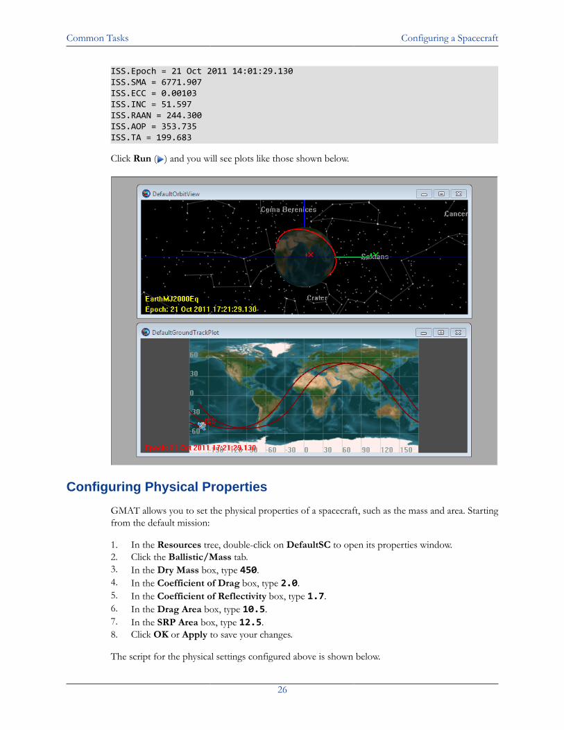
ISS.Epoch = 21 Oct 2011 14:01:29.130ISS.SMA = 6771.907ISS.ECC = 0.00103ISS.INC = 51.597ISS.RAAN = 244.300ISS.AOP = 353.735ISS.TA = 199.683
Click Run ( ) and you will see plots like those shown below.
Configuring Physical Properties
GMAT allows you to set the physical properties of a spacecraft, such as the mass and area. Startingfrom the default mission:
1. In the Resources tree, double-click on DefaultSC to open its properties window.2. Click the Ballistic/Mass tab.3. In the Dry Mass box, type 450.4. In the Coefficient of Drag box, type 2.0.5. In the Coefficient of Reflectivity box, type 1.7.6. In the Drag Area box, type 10.5.7. In the SRP Area box, type 12.5.8. Click OK or Apply to save your changes.
The script for the physical settings configured above is shown below.

Common Tasks Configuring a Spacecraft
27
Create Spacecraft DefaultSCDefaultSC.DryMass = 450DefaultSC.Cd = 2.0DefaultSC.Cr = 1.7DefaultSC.DragArea = 10.5DefaultSC.SRPArea = 12.5
Configuring the Attitude (Fixed)
GMAT can model a spacecraft with an attitude fixed in any defined coordinate system, includinguser-defined systems. This can be used to model nadir-pointing or inertially-pointed spacecraft.
For example, follow these instructions to set the attitude of the default spacecraft using Euler anglerotations from the built-in EarthMJ2000Eq inertial coordinate system. Starting from the defaultmission:
1. In the Resources tree, double-click DefaultSC to open its properties window.2. Click the Attitude tab.3. In the Attitude Model list, select CoordinateSystemFixed.4. In the Coordinate System list, select EarthMJ2000Eq.5. In the Attitude Initial Conditions area, in the Attitude State Type box, select Euler Angles.6. In the Euler Angle 1 box, type 123.7. In the Euler Angle 2 box, type 45.8. In the Euler Angle 3 box, type 157.9. Click Run ( ). The spacecraft should now be inertially pointed in the graphics window.
Configuring the Attitude (Spinner)
GMAT has a special attitude model that makes it easy to set up a spacecraft that spins about the axesof any defined coordinate system. The steps below define a spacecraft-centered coordinate systemwith axes rotating with the Sun-Earth line, then define a spacecraft as spinning about the X-axis ofthat system. Starting from the default mission:
First, define the Solar coordinate system:
1. In the Resources tree, right click Coordinate Systems and click Add Coordinate System.2. In the Coordinate System Name box, type Solar.3. In the Origin list, select DefaultSC.4. In the Type list, select ObjectReferenced.5. Set the Primary body to Sun, and the Secondary body to Earth.6. Set the X axis to -R and the Z axis to N. Leave the Y axis at its default blank value.
Now set the default spacecraft to spin about the X-axis of the Solar coordinate system:
1. In the Resources tree, double-click DefaultSC to open its properties window.2. Click the Attitude tab.3. In the Attitude Model list, select Spinner. This enables the Attitude Rate Initial Conditions
properties.4. In the Euler Angle Sequence box, select 123. This maps the first Euler angle rotation to the
X-axis of the coordinate system.

Common Tasks Configuring a Spacecraft
28
5. In the Attitude Rate State Type list, select EulerAngleRates.6. In the Euler Angle Rate 1 box, type 180.7. Click Run ( ). In the graphics window, you will see the spacecraft spinning about the Sun-
Earth line.
Common Tasks Propagating a Spacecraft
29
Propagating a SpacecraftConfiguring the Force Model
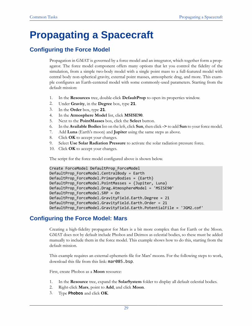
Propagation in GMAT is governed by a force model and an integrator, which together form a prop-agator. The force model component offers many options that let you control the fidelity of thesimulation, from a simple two-body model with a single point mass to a full-featured model withcentral body non-spherical gravity, external point masses, atmospheric drag, and more. This exam-ple configures an Earth-centered model with some commonly-used parameters. Starting from thedefault mission:
1. In the Resources tree, double-click DefaultProp to open its properties window.2. Under Gravity, in the Degree box, type 21.3. In the Order box, type 21.4. In the Atmosphere Model list, click MSISE90.5. Next to the PointMasses box, click the Select button.6. In the Available Bodies list on the left, click Sun, then click -> to add Sun to your force model.7. Add Luna (Earth's moon) and Jupiter using the same steps as above.8. Click OK to accept your changes.9. Select Use Solar Radiation Pressure to activate the solar radiation pressure force.10. Click OK to accept your changes.
The script for the force model configured above is shown below.
Create ForceModel DefaultProp_ForceModelDefaultProp_ForceModel.CentralBody = EarthDefaultProp_ForceModel.PrimaryBodies = {Earth}DefaultProp_ForceModel.PointMasses = {Jupiter, Luna}DefaultProp_ForceModel.Drag.AtmosphereModel = 'MSISE90'DefaultProp_ForceModel.SRP = OnDefaultProp_ForceModel.GravityField.Earth.Degree = 21DefaultProp_ForceModel.GravityField.Earth.Order = 21DefaultProp_ForceModel.GravityField.Earth.PotentialFile = 'JGM2.cof'
Configuring the Force Model: Mars
Creating a high-fidelity propagator for Mars is a bit more complex than for Earth or the Moon.GMAT does not by default include Phobos and Deimos as celestial bodies, so these must be addedmanually to include them in the force model. This example shows how to do this, starting from thedefault mission.
This example requires an external ephemeris file for Mars' moons. For the following steps to work,download this file from this link: mar085.bsp.
First, create Phobos as a Moon resource:
1. In the Resource tree, expand the SolarSystem folder to display all default celestial bodies.2. Right-click Mars, point to Add, and click Moon.3. Type Phobos and click OK.
Common Tasks Propagating a Spacecraft
30
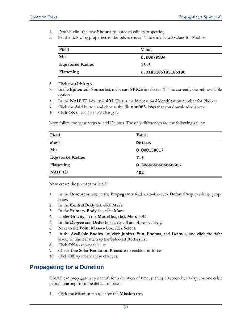
4. Double-click the new Phobos resource to edit its properties.5. Set the following properties to the values shown. These are actual values for Phobos:
Field Value
Mu 0.00070934Equatorial Radius 13.5Flattening 0.3185185185185186
6. Click the Orbit tab.7. In the Ephemeris Source list, make sure SPICE is selected. This is currently the only available
option.8. In the NAIF ID box, type 401. This is the international identification number for Phobos.9. Click the Add button and choose the file mar085.bsp that you downloaded above.10. Click OK to accept these changes.
Now follow the same steps to add Deimos. The only differences are the following values:
Field Value
Name DeimosMu 0.000158817Equatorial Radius 7.5Flattening 0.3066666666666666NAIF ID 402
Now create the propagator itself:
1. In the Resources tree, in the Propagators folder, double-click DefaultProp to edit its prop-erties.
2. In the Central Body list, click Mars.3. In the Primary Body list, click Mars.4. Under Gravity, in the Model list, click Mars-50C.5. In the Degree and Order boxes, type 4 and 4, respectively.6. Next to the Point Masses box, click Select.7. In the Available Bodies list, click Jupiter, Sun, Phobos, and Deimos, and click the right
arrow to transfer them to the Selected Bodies list.8. Click OK to accept this list.9. Check Use Solar Radiation Pressure to enable this force.10. Click OK to accept these changes.
Propagating for a Duration
GMAT can propagate a spacecraft for a duration of time, such as 60 seconds, 10 days, or one orbitperiod. Starting from the default mission:
1. Click the Mission tab to show the Mission tree.
Common Tasks Propagating a Spacecraft
31
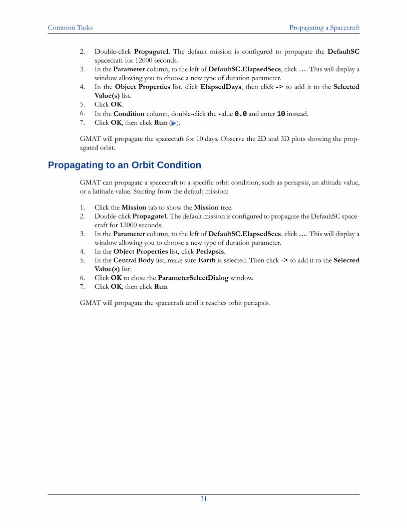
2. Double-click Propagate1. The default mission is configured to propagate the DefaultSCspacecraft for 12000 seconds.
3. In the Parameter column, to the left of DefaultSC.ElapsedSecs, click …. This will display awindow allowing you to choose a new type of duration parameter.
4. In the Object Properties list, click ElapsedDays, then click -> to add it to the SelectedValue(s) list.
5. Click OK.6. In the Condition column, double-click the value 0.0 and enter 10 instead.7. Click OK, then click Run ( ).
GMAT will propagate the spacecraft for 10 days. Observe the 2D and 3D plots showing the prop-agated orbit.
Propagating to an Orbit Condition
GMAT can propagate a spacecraft to a specific orbit condition, such as periapsis, an altitude value,or a latitude value. Starting from the default mission:
1. Click the Mission tab to show the Mission tree.2. Double-click Propagate1. The default mission is configured to propagate the DefaultSC space-
craft for 12000 seconds.3. In the Parameter column, to the left of DefaultSC.ElapsedSecs, click …. This will display a
window allowing you to choose a new type of duration parameter.4. In the Object Properties list, click Periapsis.5. In the Central Body list, make sure Earth is selected. Then click -> to add it to the Selected
Value(s) list.6. Click OK to close the ParameterSelectDialog window.7. Click OK, then click Run.
GMAT will propagate the spacecraft until it reaches orbit periapsis.
Common Tasks Reporting Data
32
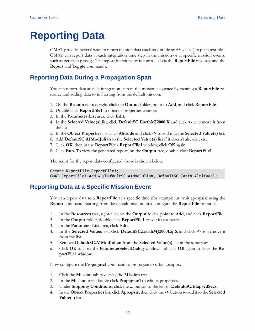
Reporting DataGMAT provides several ways to report mission data (such as altitude or ΔV values) to plain text files.GMAT can report data at each integration time step in the mission or at specific mission events,such as periapsis passage. The report functionality is controlled via the ReportFile resource and theReport and Toggle commands.
Reporting Data During a Propagation Span
You can report data at each integration step in the mission sequence by creating a ReportFile re-source and adding data to it. Starting from the default mission:
1. On the Resources tree, right-click the Output folder, point to Add, and click ReportFile.2. Double-click ReportFile1 to open its properties window.3. In the Parameter List area, click Edit.4. In the Selected Value(s) list, click DefaultSC.EarthMJ2000.X and click <- to remove it from
the list.5. In the Object Properties list, click Altitude and click -> to add it to the Selected Value(s) list.6. Add DefaultSC.A1ModJulian to the Selected Value(s) list if it doesn’t already exist.7. Click OK, then in the ReportFile - ReportFile1 window, click OK again.8. Click Run. To view the generated report, on the Output tree, double-click ReportFile1.
The script for the report data configured above is shown below.
Create ReportFile ReportFile1;GMAT ReportFile1.Add = {DefaultSC.A1ModJulian, DefaultSC.Earth.Altitude};
Reporting Data at a Specific Mission Event
You can report data to a ReportFile at a specific time (for example, at orbit apoapsis) using theReport command. Starting from the default mission, first configure the ReportFile resource:
1. In the Resources tree, right-click on the Output folder, point to Add, and click ReportFile.2. In the Output folder, double-click ReportFile1 to edit its properties.3. In the Parameter List area, click Edit.4. In the Selected Values list, click DefaultSC.EarthMJ2000Eq.X and click <- to remove it
from the list.5. Remove DefaultSC.A1ModJulian from the Selected Value(s) list in the same way.6. Click OK to close the ParameterSelectDialog window and click OK again to close the Re-
portFile1 window.
Now configure the Propagate1 command to propagate to orbit apoapsis:
1. Click the Mission tab to display the Mission tree.2. In the Mission tree, double-click Propagate1 to edit its properties.3. Under Stopping Conditions, click the ... button to the left of DefaultSC.ElapsedSecs.4. In the Object Properties list, click Apoapsis, then click the -> button to add it to the Selected
Value(s) list.
Common Tasks Reporting Data
33
5. Click OK to close the ParameterSelectDialog window, then click OK again to close the Prop-agate1 window.
Finally, add a Report command:
1. In the Mission tree, right-click Propagate1, point to Insert After, and click Report.2. Double-click Report1 to edit its properties, then click the View button.3. Click the <= button to remove all items from the Selected Value(s) list.4. In the Object Properties list, click TA, then click the -> button to add it to the Selected
Value(s) list.5. Add Altitude to the Selected Value(s) list in the same way.6. Click OK to close the ParameterSelectDialog window, then click OK to close the Report1
window.7. Click Run ( ) to run the mission.8. Click the Output tab to show the Output tree.9. In the Reports folder, double-click ReportFile1 to see the requested data.
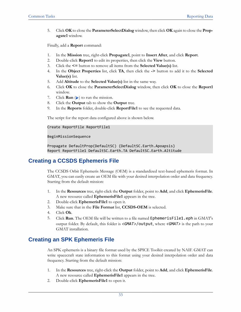
The script for the report data configured above is shown below.
Create ReportFile ReportFile1
BeginMissionSequence
Propagate DefaultProp(DefaultSC) {DefaultSC.Earth.Apoapsis}Report ReportFile1 DefaultSC.Earth.TA DefaultSC.Earth.Altitude
Creating a CCSDS Ephemeris File
The CCSDS Orbit Ephemeris Message (OEM) is a standardized text-based ephemeris format. InGMAT, you can easily create an OEM file with your desired interpolation order and data frequency.Starting from the default mission:
1. In the Resources tree, right-click the Output folder, point to Add, and click EphemerisFile.A new resource called EphemerisFile1 appears in the tree.
2. Double-click EphemerisFile1 to open it.3. Make sure that in the File Format list, CCSDS-OEM is selected.4. Click Ok.5. Click Run. The OEM file will be written to a file named EphemerisFile1.eph in GMAT's
output folder. By default, this folder is <GMAT>/output, where <GMAT> is the path to yourGMAT installation.
Creating an SPK Ephemeris File
An SPK ephemeris is a binary file format used by the SPICE Toolkit created by NAIF. GMAT canwrite spacecraft state information to this format using your desired interpolation order and datafrequency. Starting from the default mission:
1. In the Resources tree, right-click the Output folder, point to Add, and click EphemerisFile.A new resource called EphemerisFile1 appears in the tree.
2. Double-click EphemerisFile1 to open it.

Common Tasks Reporting Data
34
3. In the File Format list, click SPK.4. In the File Name box, replace the default value with EphemerisFile1.bsp. An SPK
ephemeris requires the .bsp extension.5. Click Ok.6. Click Run. The SPK file will be written to a file named EphemerisFile1.bsp in GMAT's
output folder.
Common Tasks Visualizing Data
35
Visualizing DataManipulating the 3D Orbit View
GMAT's OrbitView resource offers a three-dimensional realistic view of your mission trajectoryin any coordinate system or viewpoint you choose. The view itself can be manipulated using themouse. Starting from the default mission:
1. Click Run. This will run the mission and will result in a DefaultOrbitView window and aDefaultGroundTrackPlot window on the GMAT desktop. The default view is centered at theEarth, in an Earth-centered inertial reference frame.
2. With the left mouse button, drag in the DefaultOrbitView window. This will rotate the viewabout the center of the active coordinate system (in this case, the center of the Earth).
3. With the right mouse button, drag left-to-right. This will zoom the view out from the centerof the active coordinate system. Dragging right-to-left will zoom the view in.
4. With the wheel button (or middle button), drag up and down. This will rotate the view aboutan axis perpendicular to the screen.
Configuring the Ground Track Plot
GMAT's ground track plot can display one or more spacecraft on a two-dimensional map of a ce-lestial body. You can choose which spacecraft are displayed, and which celestial body to use. Keepingthe Earth as the central body, let's add a second spacecraft to the default plot. Starting with thedefault mission, first add a new spacecraft:
1. Right-click the Spacecraft folder and click Add Spacecraft to add Spacecraft1.2. In the Mission tree, double-click Propagate1.3. Under Spacecraft List, click ... to the left of DefaultSC.4. In the Available SpaceObject list, click Spacecraft1 and click the -> button to move it to
the SpaceObject Selected list. Then click OK. This adds Spacecraft1 to the Spacecraft Listfor Propagate1.
5. Click Apply, then click OK.
Then add the new spacecraft to the ground track plot:
1. In the Resources tree, in the Output folder, double-click DefaultGroundTrackPlot.2. In the Selected Objects list, select Spacecraft1.3. Click OK, then click Run.
After the run is complete, the DefaultGroundTrackPlot window will show the trajectory of thedefault spacecraft and Spacecraft1 on a map of Earth.
Creating a 2D Plot
GMAT offers an XYPlot resource that allows you to visualize the relationship between multipleparameters (for example, orbit altitude and time). Starting from the default mission:
1. In the Resources tree, right-click the Output folder, point to Add, and click XYPlot.
Common Tasks Visualizing Data
36
2. Double-click the new XYPlot1 resource. The default y-axis parameter is the Cartesian "X"position of the spacecraft.
3. Click Edit Y to change the y-axis parameter.4. In the Selected Value(s) list, click DefaultSC.EarthMJ2000Eq.X and click <- to remove it
from the list.5. In the Object Properties list, click Altitude.6. In the Central Body list, make sure Earth is selected, then click -> to add it to the Selected
Value(s) list.7. Click OK in the ParameterSelectDialog window, then click OK again in the XYPlot - XY-
Plot1 window.8. Click Run.
A new plot window will appear.
Part IV. Tutorials
Table of ContentsSimple Orbit Transfer ...................................................................................................................... 38
Objective and Overview .......................................................................................................... 38Configure Maneuvers, Differential Corrector, and Graphics ......................................................... 38Configure the Mission Sequence ............................................................................................... 39Run the Mission ..................................................................................................................... 46
Tutorials Simple Orbit Transfer
38
Simple Orbit TransferAudience BeginnerLength 30 minutesPrerequisites Complete Simulating an OrbitScript File Tut_SimpleOrbitTransfer.script
Objective and Overview
Note
One of the most common problems in space mission design is to design a transferfrom one circular orbit to another circular orbit that lie within the same orbital plane.Circular coplanar transfers are used to raise low-Earth orbits that have degraded dueto the effects of atmospheric drag. They are also used to transfer from a low-Earthorbit to a geosynchronous orbit and to send spacecraft to Mars. There is a well knownsequence of maneuvers, called the Hohmann transfer, that performs a circular, coplanartransfer using the least possible amount of fuel. A Hohmann transfer employs twomaneuvers. The first maneuver raises the orbital apoapsis (or lowers orbital periapsis)to the desired altitude and places the spacecraft in an elliptical transfer orbit. At theapoapsis (or periapsis) of the elliptical transfer orbit, a second maneuver is applied tocircularize the orbit at the final altitude.
In this tutorial, we will use GMAT to perform a Hohmann transfer from a low-Earth parking orbitto a geosynchronous mission orbit. This requires a targeting sequence to determine the requiredmaneuver magnitudes to achieve the desired final orbit conditions. In order to focus on the con-figuration of the targeter, we will make extensive use of the default configurations for spacecraft,propagators, and maneuvers.
The target sequence employs two velocity-direction maneuvers and two propagation sequences. Thepurpose of the first maneuver is to raise orbit apoapsis to 42,165 km, the geosynchronous radius.The purpose of the second maneuver is to nearly circularize the orbit and yield a final eccentricityof 0.005. The basic steps of this tutorial are:
1. Create and configure a DifferentialCorrector resource.2. Modify the DefaultOrbitView to visualize the trajectory.3. Create two ImpulsiveBurn resources with default settings.4. Create a Target sequence to (1) raise apoapsis to geosynchronous altitude and (2) circularize
the orbit.5. Run the mission and analyze the results.
Configure Maneuvers, Differential Corrector, and Graphics
For this tutorial, you’ll need GMAT open, with the default mission loaded. To load the defaultmission, click New Mission ( ) or start a new GMAT session. We will use the default configurationsfor the spacecraft (DefaultSC), the propagator (DefaultProp), and the two maneuvers. DefaultSCis configured by default to a near-circular orbit, and DefaultProp is configured to use Earth as the
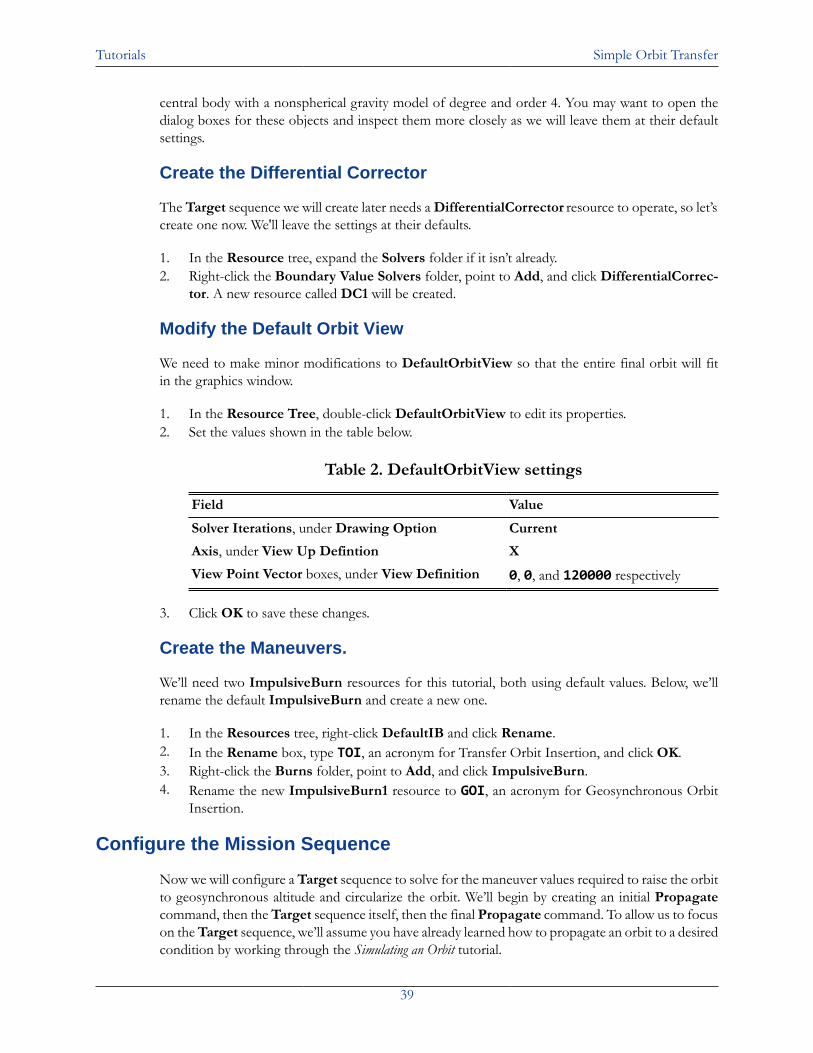
Tutorials Simple Orbit Transfer
39
central body with a nonspherical gravity model of degree and order 4. You may want to open thedialog boxes for these objects and inspect them more closely as we will leave them at their defaultsettings.
Create the Differential Corrector
The Target sequence we will create later needs a DifferentialCorrector resource to operate, so let’screate one now. We'll leave the settings at their defaults.
1. In the Resource tree, expand the Solvers folder if it isn’t already.2. Right-click the Boundary Value Solvers folder, point to Add, and click DifferentialCorrec-
tor. A new resource called DC1 will be created.
Modify the Default Orbit View
We need to make minor modifications to DefaultOrbitView so that the entire final orbit will fitin the graphics window.
1. In the Resource Tree, double-click DefaultOrbitView to edit its properties.2. Set the values shown in the table below.
Table 2. DefaultOrbitView settings
Field Value
Solver Iterations, under Drawing Option CurrentAxis, under View Up Defintion XView Point Vector boxes, under View Definition 0, 0, and 120000 respectively
3. Click OK to save these changes.
Create the Maneuvers.
We’ll need two ImpulsiveBurn resources for this tutorial, both using default values. Below, we’llrename the default ImpulsiveBurn and create a new one.
1. In the Resources tree, right-click DefaultIB and click Rename.2. In the Rename box, type TOI, an acronym for Transfer Orbit Insertion, and click OK.3. Right-click the Burns folder, point to Add, and click ImpulsiveBurn.4. Rename the new ImpulsiveBurn1 resource to GOI, an acronym for Geosynchronous Orbit
Insertion.
Configure the Mission Sequence
Now we will configure a Target sequence to solve for the maneuver values required to raise the orbitto geosynchronous altitude and circularize the orbit. We’ll begin by creating an initial Propagatecommand, then the Target sequence itself, then the final Propagate command. To allow us to focuson the Target sequence, we’ll assume you have already learned how to propagate an orbit to a desiredcondition by working through the Simulating an Orbit tutorial.
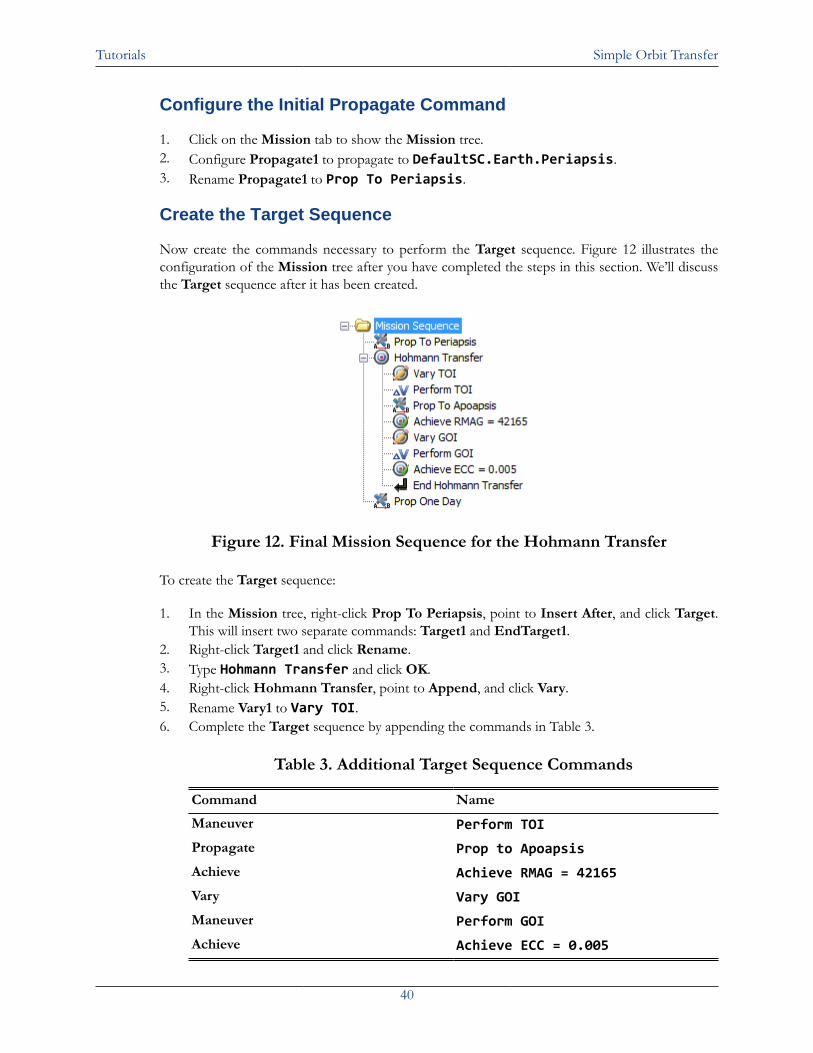
Tutorials Simple Orbit Transfer
40
Configure the Initial Propagate Command
1. Click on the Mission tab to show the Mission tree.2. Configure Propagate1 to propagate to DefaultSC.Earth.Periapsis.3. Rename Propagate1 to Prop To Periapsis.
Create the Target Sequence
Now create the commands necessary to perform the Target sequence. Figure 12 illustrates theconfiguration of the Mission tree after you have completed the steps in this section. We’ll discussthe Target sequence after it has been created.
Figure 12. Final Mission Sequence for the Hohmann Transfer
To create the Target sequence:
1. In the Mission tree, right-click Prop To Periapsis, point to Insert After, and click Target.This will insert two separate commands: Target1 and EndTarget1.
2. Right-click Target1 and click Rename.3. Type Hohmann Transfer and click OK.4. Right-click Hohmann Transfer, point to Append, and click Vary.5. Rename Vary1 to Vary TOI.6. Complete the Target sequence by appending the commands in Table 3.
Table 3. Additional Target Sequence Commands
Command Name
Maneuver Perform TOIPropagate Prop to ApoapsisAchieve Achieve RMAG = 42165Vary Vary GOIManeuver Perform GOIAchieve Achieve ECC = 0.005
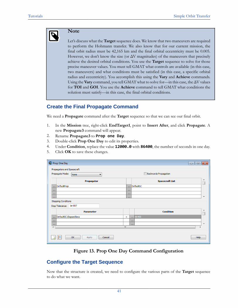
Tutorials Simple Orbit Transfer
41
Note
Let’s discuss what the Target sequence does. We know that two maneuvers are requiredto perform the Hohmann transfer. We also know that for our current mission, thefinal orbit radius must be 42,165 km and the final orbital eccentricity must be 0.005.However, we don’t know the size (or ΔV magnitudes) of the maneuvers that preciselyachieve the desired orbital conditions. You use the Target sequence to solve for thoseprecise maneuver values. You must tell GMAT what controls are available (in this case,two maneuvers) and what conditions must be satisfied (in this case, a specific orbitalradius and eccentricity). You accomplish this using the Vary and Achieve commands.Using the Vary command, you tell GMAT what to solve for—in this case, the ΔV valuesfor TOI and GOI. You use the Achieve command to tell GMAT what conditions thesolution must satisfy—in this case, the final orbital conditions.
Create the Final Propagate Command
We need a Propagate command after the Target sequence so that we can see our final orbit.
1. In the Mission tree, right-click EndTarget1, point to Insert After, and click Propagate. Anew Propagate3 command will appear.
2. Rename Propagate3 to Prop one Day.3. Double-click Prop One Day to edit its properties.4. Under Condition, replace the value 12000.0 with 86400, the number of seconds in one day.5. Click OK to save these changes.
Figure 13. Prop One Day Command Configuration
Configure the Target Sequence
Now that the structure is created, we need to configure the various parts of the Target sequenceto do what we want.
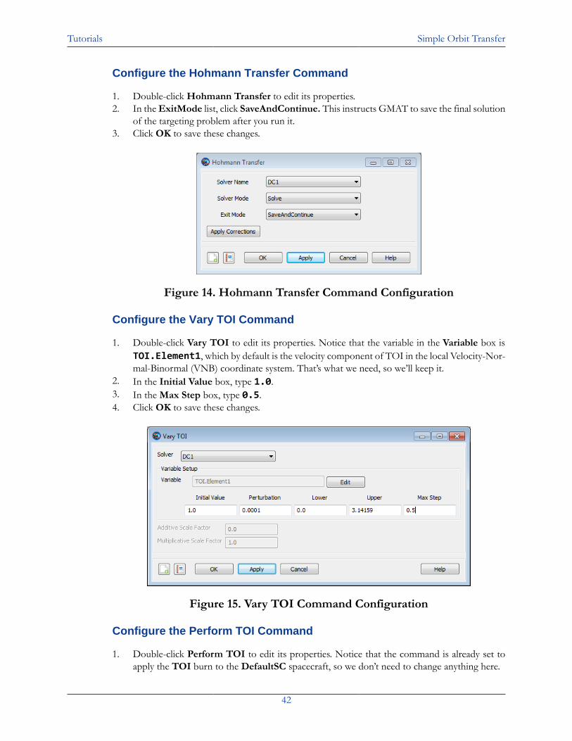
Tutorials Simple Orbit Transfer
42
Configure the Hohmann Transfer Command
1. Double-click Hohmann Transfer to edit its properties.2. In the ExitMode list, click SaveAndContinue. This instructs GMAT to save the final solution
of the targeting problem after you run it.3. Click OK to save these changes.
Figure 14. Hohmann Transfer Command Configuration
Configure the Vary TOI Command
1. Double-click Vary TOI to edit its properties. Notice that the variable in the Variable box isTOI.Element1, which by default is the velocity component of TOI in the local Velocity-Nor-mal-Binormal (VNB) coordinate system. That’s what we need, so we’ll keep it.
2. In the Initial Value box, type 1.0.3. In the Max Step box, type 0.5.4. Click OK to save these changes.
Figure 15. Vary TOI Command Configuration
Configure the Perform TOI Command
1. Double-click Perform TOI to edit its properties. Notice that the command is already set toapply the TOI burn to the DefaultSC spacecraft, so we don’t need to change anything here.
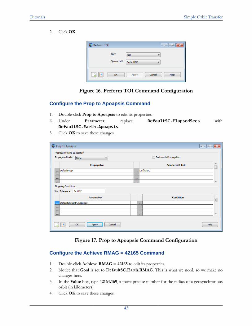
Tutorials Simple Orbit Transfer
43
2. Click OK.
Figure 16. Perform TOI Command Configuration
Configure the Prop to Apoapsis Command
1. Double-click Prop to Apoapsis to edit its properties.2. Under Parameter, replace DefaultSC.ElapsedSecs with
DefaultSC.Earth.Apoapsis.3. Click OK to save these changes.
Figure 17. Prop to Apoapsis Command Configuration
Configure the Achieve RMAG = 42165 Command
1. Double-click Achieve RMAG = 42165 to edit its properties.2. Notice that Goal is set to DefaultSC.Earth.RMAG. This is what we need, so we make no
changes here.3. In the Value box, type 42164.169, a more precise number for the radius of a geosynchronous
orbit (in kilometers).4. Click OK to save these changes.
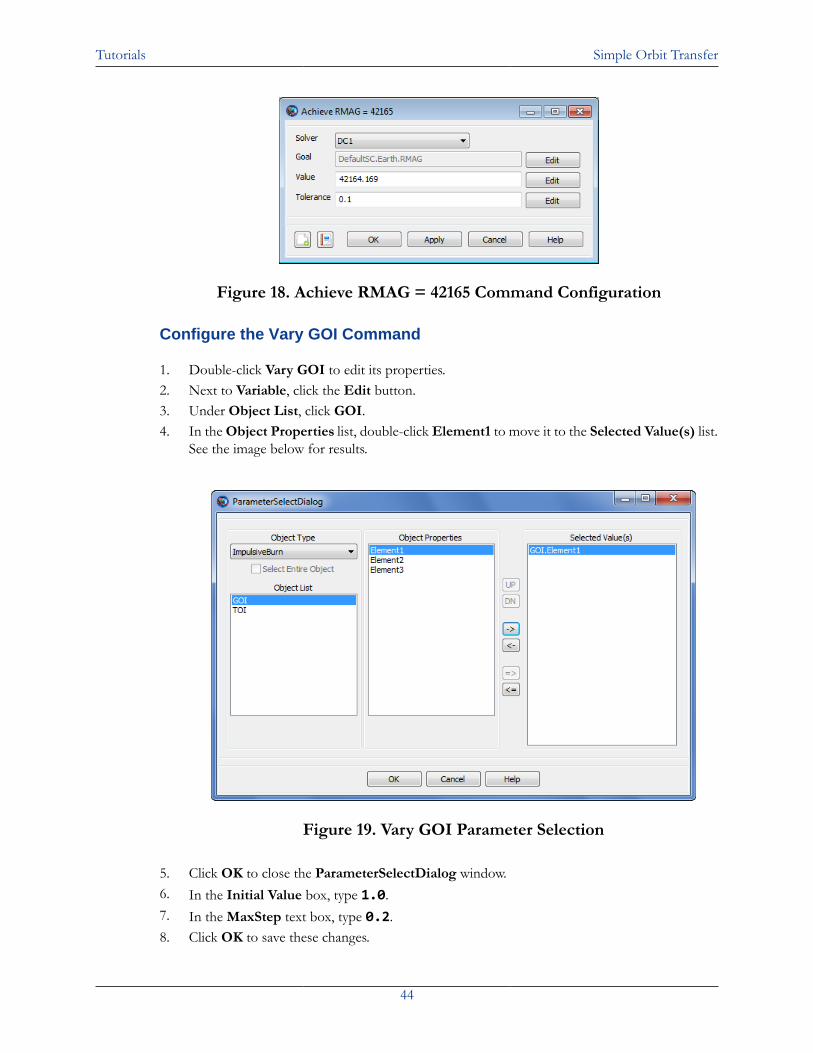
Tutorials Simple Orbit Transfer
44
Figure 18. Achieve RMAG = 42165 Command Configuration
Configure the Vary GOI Command
1. Double-click Vary GOI to edit its properties.2. Next to Variable, click the Edit button.3. Under Object List, click GOI.4. In the Object Properties list, double-click Element1 to move it to the Selected Value(s) list.
See the image below for results.
Figure 19. Vary GOI Parameter Selection
5. Click OK to close the ParameterSelectDialog window.6. In the Initial Value box, type 1.0.7. In the MaxStep text box, type 0.2.8. Click OK to save these changes.
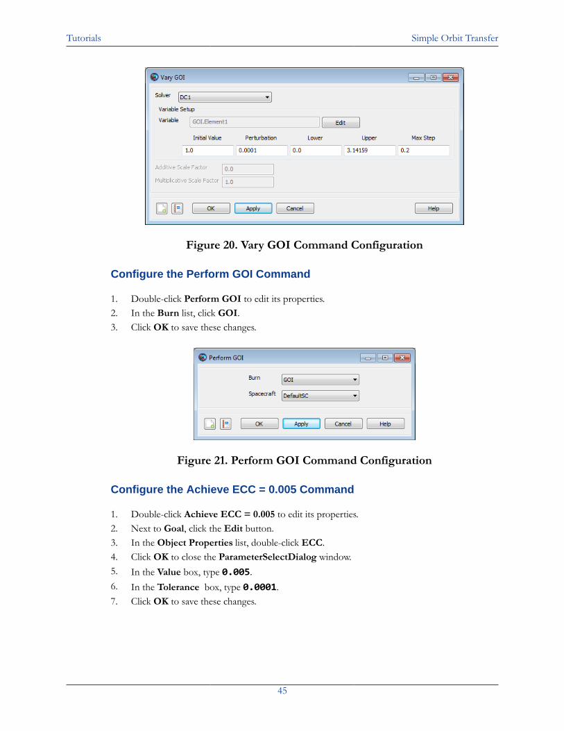
Tutorials Simple Orbit Transfer
45
Figure 20. Vary GOI Command Configuration
Configure the Perform GOI Command
1. Double-click Perform GOI to edit its properties.2. In the Burn list, click GOI.3. Click OK to save these changes.
Figure 21. Perform GOI Command Configuration
Configure the Achieve ECC = 0.005 Command
1. Double-click Achieve ECC = 0.005 to edit its properties.2. Next to Goal, click the Edit button.3. In the Object Properties list, double-click ECC.4. Click OK to close the ParameterSelectDialog window.5. In the Value box, type 0.005.6. In the Tolerance box, type 0.0001.7. Click OK to save these changes.
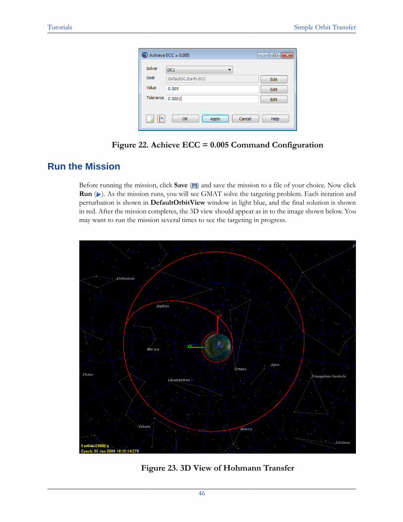
Tutorials Simple Orbit Transfer
46
Figure 22. Achieve ECC = 0.005 Command Configuration
Run the Mission
Before running the mission, click Save ( ) and save the mission to a file of your choice. Now clickRun ( ). As the mission runs, you will see GMAT solve the targeting problem. Each iteration andperturbation is shown in DefaultOrbitView window in light blue, and the final solution is shownin red. After the mission completes, the 3D view should appear as in to the image shown below. Youmay want to run the mission several times to see the targeting in progress.
Figure 23. 3D View of Hohmann Transfer

Tutorials Simple Orbit Transfer
47
If you were to continue developing this mission, you can store the final solution of the Targetsequence as the initial conditions of the TOI and GOI resources themselves, so that if you makesmall changes, the subsequent runs will take less time. To do this, follow these steps:
1. In the Mission tree, double-click Hohmann Transfer to edit its properties.2. Click Apply Corrections.3. Now re-run the mission. If you inspect the results in the message window, you will see that
the Target sequence converges in one iteration because you stored the solution as the initialcondition.
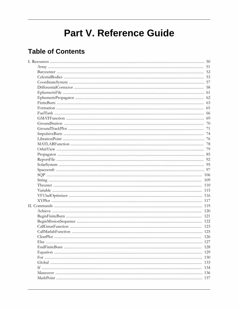
Part V. Reference Guide
Table of ContentsI. Resources .................................................................................................................................... 50
Array ..................................................................................................................................... 51Barycenter .............................................................................................................................. 52CelestialBodies ........................................................................................................................ 53CoordinateSystem .................................................................................................................... 57DifferentialCorrector ............................................................................................................... 58EphemerisFile ......................................................................................................................... 61EphemerisPropagator .............................................................................................................. 62FiniteBurn .............................................................................................................................. 63Formation .............................................................................................................................. 65FuelTank ................................................................................................................................ 66GMATFunction ...................................................................................................................... 69GroundStation ........................................................................................................................ 70GroundTrackPlot .................................................................................................................... 71ImpulsiveBurn ........................................................................................................................ 74LibrationPoint ......................................................................................................................... 76MATLABFunction .................................................................................................................. 78OrbitView .............................................................................................................................. 79Propagator .............................................................................................................................. 85ReportFile .............................................................................................................................. 92SolarSystem ............................................................................................................................ 95Spacecraft ............................................................................................................................... 97SQP ..................................................................................................................................... 106String ................................................................................................................................... 109Thruster ............................................................................................................................... 110Variable ................................................................................................................................ 115VF13adOptimizer .................................................................................................................. 116XYPlot ................................................................................................................................. 117
II. Commands ............................................................................................................................... 119Achieve ................................................................................................................................ 120BeginFiniteBurn .................................................................................................................... 121BeginMissionSequence ........................................................................................................... 122CallGmatFunction ................................................................................................................. 123CallMatlabFunction ................................................................................................................ 125ClearPlot .............................................................................................................................. 126Else ...................................................................................................................................... 127EndFiniteBurn ...................................................................................................................... 128Equation ............................................................................................................................... 129For ....................................................................................................................................... 130Global .................................................................................................................................. 133If ......................................................................................................................................... 134Maneuver .............................................................................................................................. 136MarkPoint ............................................................................................................................. 137
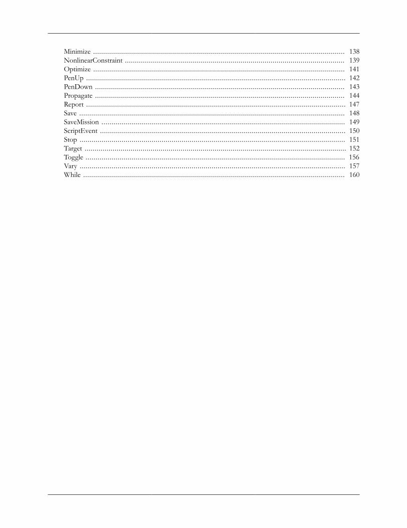
Minimize .............................................................................................................................. 138NonlinearConstraint .............................................................................................................. 139Optimize .............................................................................................................................. 141PenUp .................................................................................................................................. 142PenDown ............................................................................................................................. 143Propagate ............................................................................................................................. 144Report .................................................................................................................................. 147Save ..................................................................................................................................... 148SaveMission .......................................................................................................................... 149ScriptEvent ........................................................................................................................... 150Stop ..................................................................................................................................... 151Target ................................................................................................................................... 152Toggle .................................................................................................................................. 156Vary ..................................................................................................................................... 157While ................................................................................................................................... 160

Reference Guide Resources
50
Resources
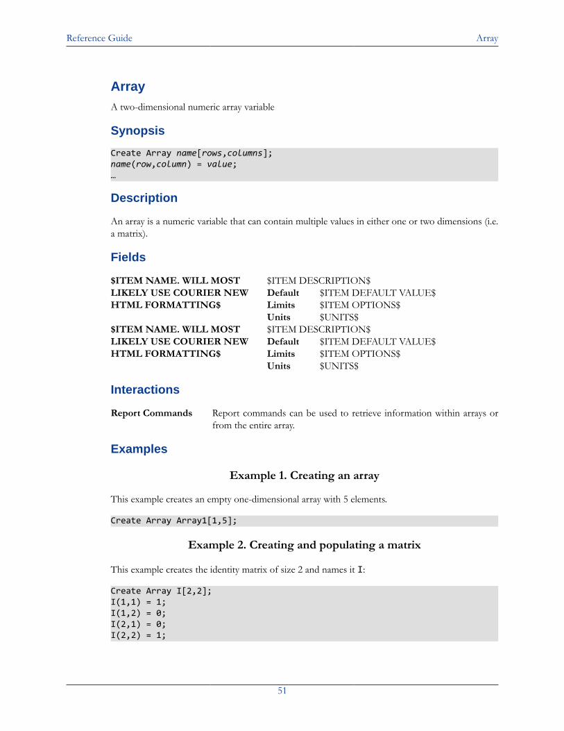
Reference Guide Array
51
ArrayA two-dimensional numeric array variable
Synopsis
Create Array name[rows,columns];name(row,column) = value;…
Description
An array is a numeric variable that can contain multiple values in either one or two dimensions (i.e.a matrix).
Fields
$ITEM NAME. WILL MOSTLIKELY USE COURIER NEWHTML FORMATTING$
$ITEM DESCRIPTION$Default $ITEM DEFAULT VALUE$Limits $ITEM OPTIONS$Units $UNITS$
$ITEM NAME. WILL MOSTLIKELY USE COURIER NEWHTML FORMATTING$
$ITEM DESCRIPTION$Default $ITEM DEFAULT VALUE$Limits $ITEM OPTIONS$Units $UNITS$
Interactions
Report Commands Report commands can be used to retrieve information within arrays orfrom the entire array.
Examples
Example 1. Creating an array
This example creates an empty one-dimensional array with 5 elements.
Create Array Array1[1,5];
Example 2. Creating and populating a matrix
This example creates the identity matrix of size 2 and names it I:
Create Array I[2,2];I(1,1) = 1;I(1,2) = 0;I(2,1) = 0;I(2,2) = 1;
Reference Guide Barycenter
52
BarycenterA barycenter.
Synopsis
Create Barycenter namename.BodyNames = {bodyName1,bodyName2,...,bodyNameN}
Description
A barycenter is the center of mass of one or more celestial bodies and can be used as the origin ofa CoordinateSystem, a reference point in an OrbitView, or as one of the points in a LibrationPoint.
Fields
BodyNames The BodyNames field is a list that contains the bodies used to define abarycenter. In a script, the list must be surrounded by curly braces. (i.e.BaryCenterName.BodyNames = { Earth, Luna }) Default Earth, LunaLimits Sun, Mercury, Venus, Earth, Luna, Mars, Jupiter, Saturn, Uranus, Nep-
tune, Pluto, or any user-defined celestial body. At least one body mustbe selected!
Units N/A
Interactions
Coordinate Systems Interacts with the barycenter object selecting it as the origin of thecoordinate system or as a primary or secondary point for definingthe axes.
OpenGL Plot It can be selected as a celestial object to be drawn onto the plot, aView Point Reference, or the View Direction within the dialog box.
Examples
Create Barycenter EarthMoonBary;GMAT EarthMoonBary.BodyNames = {Earth, Luna};
Reference Guide CelestialBodies
53
CelestialBodies
A celestial body.
Synopsis
Create Planet namename.field = value
Description
The Celestial Bodies are the main bodies of the Solar System and the Moon. They are part of theresource tree and are under Solar System. They can be selected for a large variety of options forpoints of reference.
Fields
Fields Associated with All Celestial Bodies
Mu The Mu field allows the user to define the gravitational parameter ofa celestial body.Default 398600.4414Limits Real Number < 0Units km3/sec2.z
Equatorial Radius The EquatorialRadius field allows the user to define the equatorial ra-dius of a celestial body.Default 6378.1363Limits Real Number < 0Units km
Flattening The Flattening field allows the user to define the mass of a celestialbody.Default 0.00335270Limits Real NumberUnits None
InitialEpoch The InitialEpoch field allows the user to define the initial epoch, inA1 Modified Julian Date, for a celestial body. The initial epoch is onlyused when the user selects Analytic for the Ephemeris field on thesolar system. In this case, GMAT solves Kepler's problem to determinetheposition and velocity of a celestial body, using the initial epoch andstate information described below.Default 21544.500371Limits Real NumberUnits A1ModJulian
SMA The SMA field allows the user to define the semimajor axis of a celestialbody's orbit about its central body. (Only used when the user selectsAnalytic for the Ephemeris field on the Solar System.)Default 149653978.978377Limits Real Number ≥ 0
Reference Guide CelestialBodies
54
Units kmECC The ECC field allows the user to define the eccentricity of a celestial
body's orbit about its central body. (Only used when the user selectsAnalytic for the Ephemeris field on the Solar System.)Default 0.017046Limits Real Number ≥ 0Units None
INC The INC field allows the user to define the inclination of a celestialbody's orbit about its central body, in the FK5 coordinate system. (Onlyused when the user selects Analytic for the Ephemeris field on the SolarSystem.)Default 23.439034Limits Real NumberUnits deg
RAAN The RAAN field allows the user to define the right ascension of theascending node of a celestialbody's orbit about its central body, in theFK5 coordinate system. (Only used when the user selects Analytic forthe Ephemeris field on the Solar System.)Default 0.000186Limits Real NumberUnits deg
AOP The AOP field allows the user to define the argument of periapsis ofa celestial body's orbit about its central body, in the FK5 coordinatesystem. (Only used when the user selects Analytic for the Ephemerisfield on the Solar System.)Default 101.741639Limits Real NumberUnits deg
TA The TA field allows the user to define the true anomaly of a celestialbody's orbit about its central body. (Only used when the user selectsAnalytic for the Ephemeris field on the Solar System.)Default 358.127085Limits Real NumberUnits deg
Special Fields Associated with Earth
NutationUpdate Interval The NutationUpdateInterval field, on the Earth CelestialBody, determines how often GMAT updates the Nutationmatrix used in FK5 reduction. If NutationUpdateInterval isset to zero, the Nutation is updated every time a requestis made to calculate the orientation of the Earth. If Nuta-tionUpdateInterval is set to a real number greater than zero,then GMAT only updates the Nutation matrix if the numberof seconds defined by NutationUpdateInterval have elapsedsince the last request for the Earth's orientation data.Default 60Limits Real Number ≥ 0Units sec
Reference Guide CelestialBodies
55
Special Fields Associated with Luna
RotationData Source The RotationDataSource, on the Luna Celestial Body, determineswhat source GMAT uses to obtain data describing the orientation ofthe moon with respect to the FK5 system. The RotationDataSourcefield is only used for lunar orientation data when calculating moon-based coordinate systems with the axes types of {Fixed} and {Equa-tor}.Default DE405Limits DE405, IAU2002Units N/A
Interactions
Coordinate System Interacts with the celestial body in that the body can be selected as theorigin of the coordinate system or as a primary or secondary point fordefining the axes.
OpenGL plot Interacts with a celestial body in a number of ways. It can be selectedto be drawn onto the plot, with the color of the orbit an option. Acelestial body can also be selected as the View Point Reference or theView Direction.
Propagator Can interact with a celestial body in a number of ways. Under the ForceModel heading, any celestial body can be chosen for use as the centralbody, as the primary bodies, and the secondary bodies.
Bary Center Can interact with celestial bodies in that a bary center is calculated usingsome number of celestial bodies which can be selected.
Libration point Can interact with celestial bodies in that a libration point is calculatedusing two celestial bodies which can be selected.
Spacecraft Interacts with celestial bodies in that for a number of parameters de-scribe how the spacecraft is positioned in relation to a celestial body.This can include the periapsis, apoapsis, and altitude, as well as a greatmany of other parameters.
Examples
Create Planet Earth;GMAT Earth.BodyType = 'Planet';GMAT Earth.Mass = 5.973331957140716e+024;GMAT Earth.EquatorialRadius = 6378.1363;GMAT Earth.Flattening = 0.0033527;GMAT Earth.PolarRadius = 6356.75232242699;GMAT Earth.Mu = 398600.4415;GMAT Earth.PosVelSource = 'DE_405';GMAT Earth.State = [ 0 0 0 0 0 0 ];GMAT Earth.StateTime = 0;GMAT Earth.CentralBody = 'Sun';GMAT Earth.BodyNumber = 2;GMAT Earth.RefBodyNumber = 3;GMAT Earth.SourceFilename = './files/planetary_ephem/de/winp1941.405';GMAT Earth.SourceFile = ./files/planetary_ephem/de/winp1941.405;GMAT Earth.UsePotentialFileFlag = false;
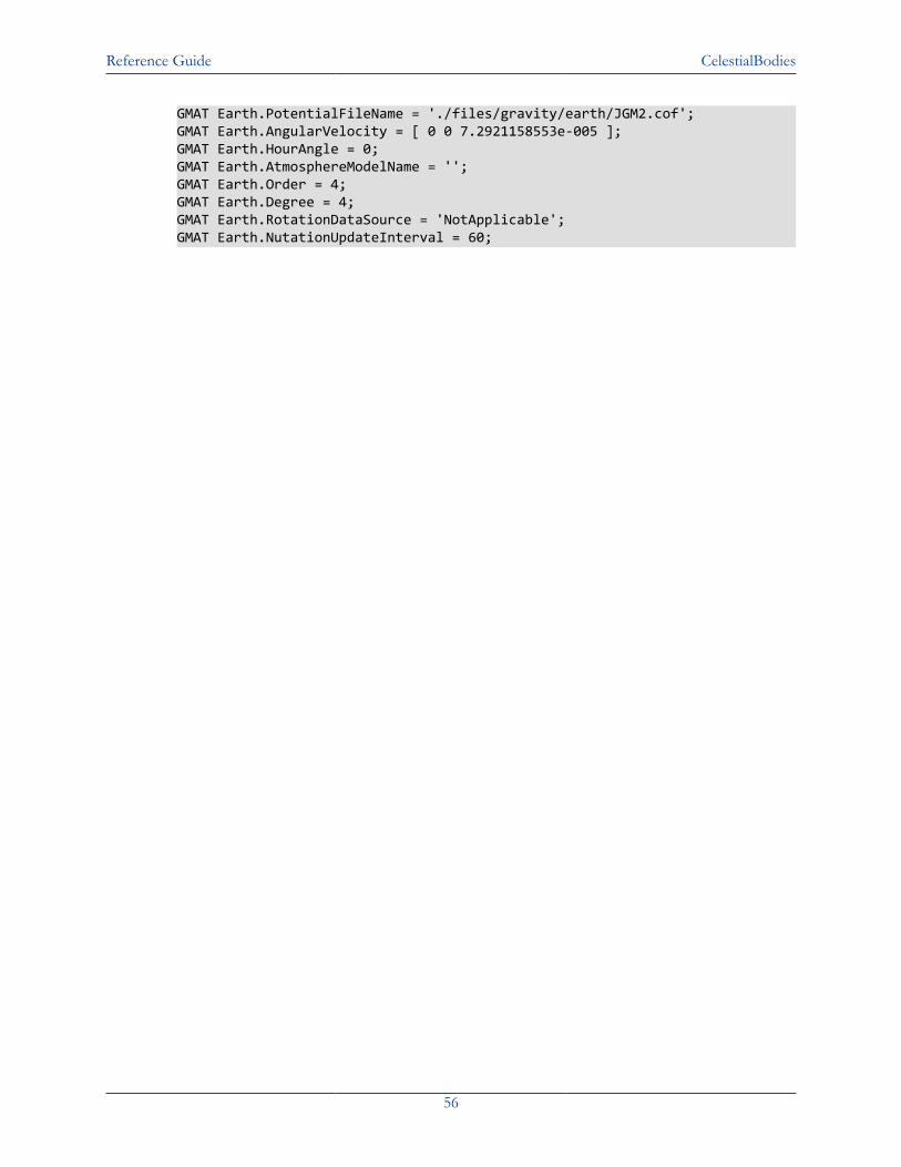
Reference Guide CelestialBodies
56
GMAT Earth.PotentialFileName = './files/gravity/earth/JGM2.cof';GMAT Earth.AngularVelocity = [ 0 0 7.2921158553e-005 ];GMAT Earth.HourAngle = 0;GMAT Earth.AtmosphereModelName = '';GMAT Earth.Order = 4;GMAT Earth.Degree = 4;GMAT Earth.RotationDataSource = 'NotApplicable';GMAT Earth.NutationUpdateInterval = 60;
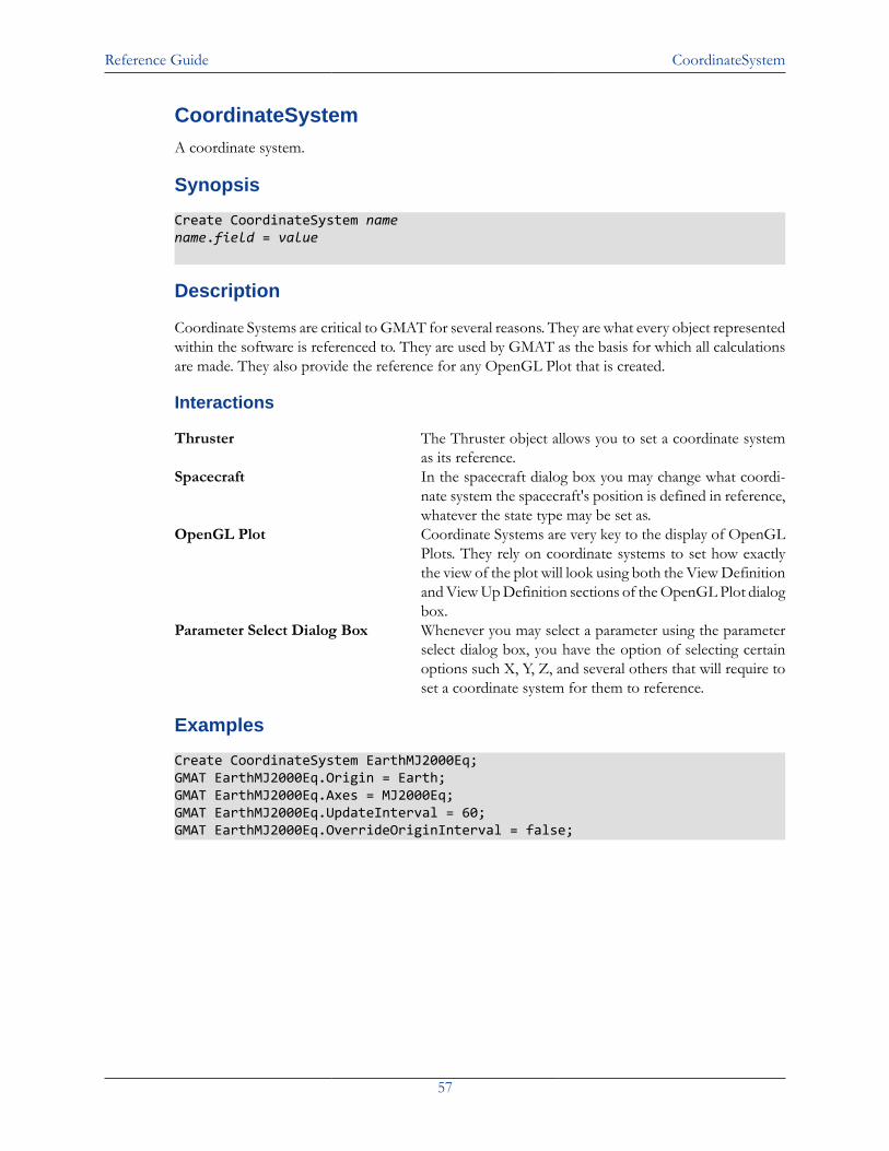
Reference Guide CoordinateSystem
57
CoordinateSystemA coordinate system.
Synopsis
Create CoordinateSystem namename.field = value
Description
Coordinate Systems are critical to GMAT for several reasons. They are what every object representedwithin the software is referenced to. They are used by GMAT as the basis for which all calculationsare made. They also provide the reference for any OpenGL Plot that is created.
Interactions
Thruster The Thruster object allows you to set a coordinate systemas its reference.
Spacecraft In the spacecraft dialog box you may change what coordi-nate system the spacecraft's position is defined in reference,whatever the state type may be set as.
OpenGL Plot Coordinate Systems are very key to the display of OpenGLPlots. They rely on coordinate systems to set how exactlythe view of the plot will look using both the View Definitionand View Up Definition sections of the OpenGL Plot dialogbox.
Parameter Select Dialog Box Whenever you may select a parameter using the parameterselect dialog box, you have the option of selecting certainoptions such X, Y, Z, and several others that will require toset a coordinate system for them to reference.
Examples
Create CoordinateSystem EarthMJ2000Eq;GMAT EarthMJ2000Eq.Origin = Earth;GMAT EarthMJ2000Eq.Axes = MJ2000Eq;GMAT EarthMJ2000Eq.UpdateInterval = 60;GMAT EarthMJ2000Eq.OverrideOriginInterval = false;
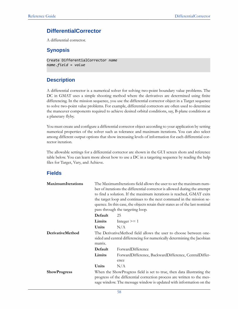
Reference Guide DifferentialCorrector
58
DifferentialCorrector
A differential corrector.
Synopsis
Create DifferentialCorrector namename.field = value
Description
A differential corrector is a numerical solver for solving two-point boundary value problems. TheDC in GMAT uses a simple shooting method where the derivatives are determined using finitedifferencing. In the mission sequence, you use the differential corrector object in a Target sequenceto solve two-point value problems. For example, differential correctors are often used to determinethe maneuver components required to achieve desired orbital conditions, say, B-plane conditions ata planetary flyby.
You must create and configure a differential corrector object according to your application by settingnumerical properties of the solver such as tolerance and maximum iterations. You can also selectamong different output options that show increasing levels of information for each differential cor-rector iteration.
The allowable settings for a differential corrector are shown in the GUI screen shots and referencetable below. You can learn more about how to use a DC in a targeting sequence by reading the helpfiles for Target, Vary, and Achieve.
Fields
MaximumIterations The MaximumIterations field allows the user to set the maximum num-ber of iterations the differential corrector is allowed during the attemptto find a solution. If the maximum iterations is reached, GMAT exitsthe target loop and continues to the next command in the mission se-quence. In this case, the objects retain their states as of the last nominalpass through the targeting loop.Default 25Limits Integer >= 1Units N/A
DerivativeMethod The DerivativeMethod field allows the user to choose between one-sided and central differencing for numerically determining the Jacobianmatrix.Default ForwardDifferenceLimits ForwardDifference, BackwardDifference, CentralDiffer-
enceUnits N/A
ShowProgress When the ShowProgress field is set to true, then data illustrating theprogress of the differential correction process are written to the mes-sage window. The message window is updated with information on the
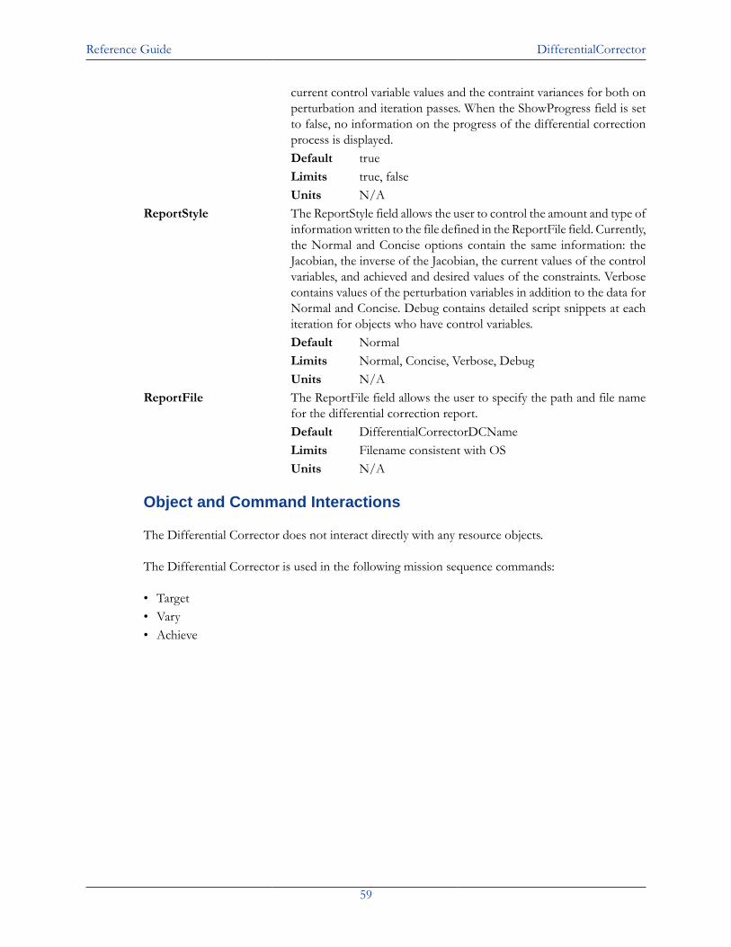
Reference Guide DifferentialCorrector
59
current control variable values and the contraint variances for both onperturbation and iteration passes. When the ShowProgress field is setto false, no information on the progress of the differential correctionprocess is displayed.Default trueLimits true, falseUnits N/A
ReportStyle The ReportStyle field allows the user to control the amount and type ofinformation written to the file defined in the ReportFile field. Currently,the Normal and Concise options contain the same information: theJacobian, the inverse of the Jacobian, the current values of the controlvariables, and achieved and desired values of the constraints. Verbosecontains values of the perturbation variables in addition to the data forNormal and Concise. Debug contains detailed script snippets at eachiteration for objects who have control variables.Default NormalLimits Normal, Concise, Verbose, DebugUnits N/A
ReportFile The ReportFile field allows the user to specify the path and file namefor the differential correction report.Default DifferentialCorrectorDCNameLimits Filename consistent with OSUnits N/A
Object and Command Interactions
The Differential Corrector does not interact directly with any resource objects.
The Differential Corrector is used in the following mission sequence commands:
• Target• Vary• Achieve
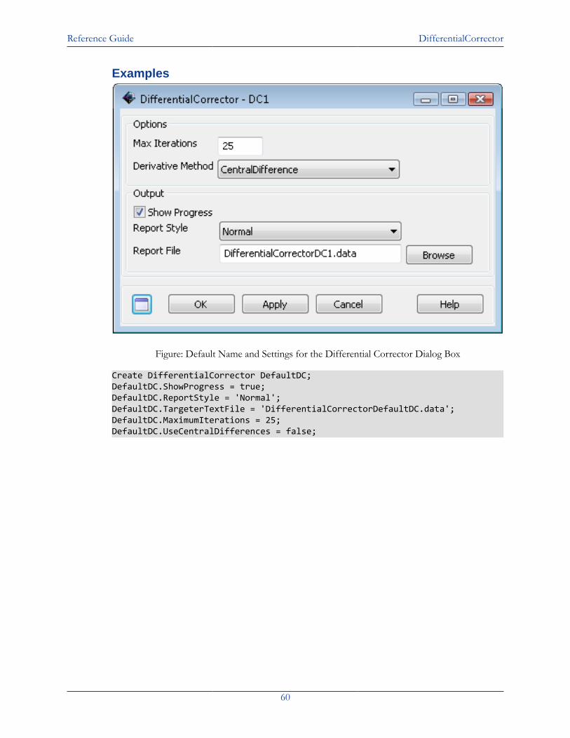
Reference Guide DifferentialCorrector
60
Examples
Figure: Default Name and Settings for the Differential Corrector Dialog Box
Create DifferentialCorrector DefaultDC;DefaultDC.ShowProgress = true;DefaultDC.ReportStyle = 'Normal';DefaultDC.TargeterTextFile = 'DifferentialCorrectorDefaultDC.data';DefaultDC.MaximumIterations = 25;DefaultDC.UseCentralDifferences = false;
Reference Guide EphemerisFile
61
EphemerisFileAn ephemeris file.
Synopsis
Under Construction.
Description
Under Construction.
Fields
Field Name Description....Type Fill This In.Default Fill This In.Limits Fill This In.Units Fill This In.
Examples
Example 3. Example Script
%
Reference Guide EphemerisPropagator
62
EphemerisPropagatorUnder Construction.
Synopsis
Under Construction.
Description
Under Construction.
Fields
Field Name Description....Type Fill This In.Default Fill This In.Limits Fill This In.Units Fill This In.
Examples
Example 4. Example Script
%
Reference Guide FiniteBurn
63
FiniteBurnA finite burn.
Synopsis
Create FiniteBurn namename.field = value
Description
The Finite Burn object is used when a continuous propulsion is desired. Impulsive burns happen in-stantaneously and through a Maneuver command, while finite burns occur until the End Finite Burncommand is reached in the mission sequence and are typically coupled with Propagate commands.
Fields
Origin Together the Origin and Axes fields describe the coordinate system inwhich a maneuver is applied. The Origin field determines the origin ofthe maneuver coordinate system. The ability to define the coordinate sys-tem locally avoids having to create many coordinate systems, associatedwith specific spacecraft, in order to perform finite maneuvers for multiplespacecraft.Default EarthLimits Any celestial body, libration point, or barycenterUnits N/A
Axes The Axes field, together with the Origin field, describe the coordinatesystem in which a finite maneuver is applied. If VNB is chosen for Axes, alocal coordinate system is created such that the x-axis points in the velocitydirection of the spacecraft, with respect to the point defined by Origin,the y-axis points in the normal direction of the spacecraft with respect toOrigin, and the z-axis completes the right-handed set.Default VNBLimits VNB, MJ2000EqUnits N/A
Thrusters The Thrusters field allows the selection of which thrusters to usewhen applying a finite maneuver. The user can select more than onethruster, from the list of thrusters previously created, by includingall thrusters in curly braces. An example is MyFiniteBurn.Thrusters =Thruster1,Thruster2,Thruster3.Default No DefaultLimits Any thruster created by userUnits N/A
BurnScaleFactor The BurnScaleFactor is used to scale the total acceleration before addingthe acceleration due to a finite burn into the sum of the accelerations of aspacecraft. The scaling is performed by taking the sum of the accelerationsapplied by all thrusters specified under the Thrusters field, and multiplyingthe total thrust by BurnScaleFactor.Default 1.0
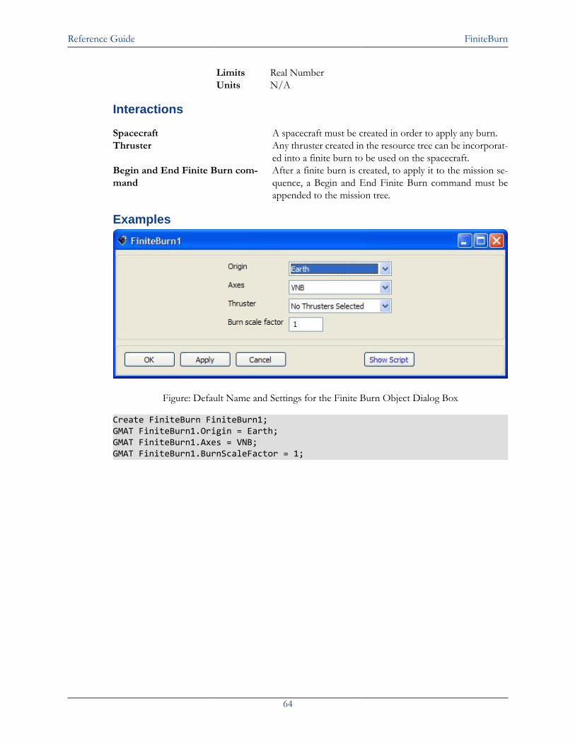
Reference Guide FiniteBurn
64
Limits Real NumberUnits N/A
Interactions
Spacecraft A spacecraft must be created in order to apply any burn.Thruster Any thruster created in the resource tree can be incorporat-
ed into a finite burn to be used on the spacecraft.Begin and End Finite Burn com-mand
After a finite burn is created, to apply it to the mission se-quence, a Begin and End Finite Burn command must beappended to the mission tree.
Examples
Figure: Default Name and Settings for the Finite Burn Object Dialog Box
Create FiniteBurn FiniteBurn1;GMAT FiniteBurn1.Origin = Earth;GMAT FiniteBurn1.Axes = VNB;GMAT FiniteBurn1.BurnScaleFactor = 1;
Reference Guide Formation
65
FormationAn ephemeris file.
Synopsis
Under Construction.
Description
Under Construction.
Fields
Field Name Description....Type Fill This In.Default Fill This In.Limits Fill This In.Units Fill This In.
Examples
Example 5. Example Script
%
Reference Guide FuelTank
66
FuelTankA fuel tank.
Synopsis
Create FuelTank namename.field = value
Description
A FuelTank is a thermodynamc model of a tank and is required for finite burn modelling or forimplusive burns that use mass depletion. The thermodynamic properties of the tank are modelledusing the ideal gas law and assume that there is no energy transfer into or out of the tank as fuel isdepleted. To use a FuelTank, you must first create the tank, and then attach it to the desired spacecraftand associate it with a thruster as shown in the examples below.
When working in the script, you must add tanks to spacecraft before the begin mission sequencecommand.
Fields
Pressure The pressure in the tank.Type Real NumberDefault 1500Limits Pressure > 0Units kPa.
Temperature The temperature of the fuel and ullage in the tank. GMAT currently assumesullage and fuel are always at the same temperature.Type Real NumberDefault 20Limits Temperature > -273.15Units C.
FuelMass The FuelMass field is the mass of fuel in the tank.
Caution
By default, GMAT will not allow the fuel mass to be negative. How-ever, occasionally in iterative processes such as targeting, a solverwill try values of a maneuver parameter that result in total fuel de-pletion. Using the default tank settings this will throw an excpep-tion stopping the run unless you set the AllowNegativeFuelMassflag to true.
Type Real NumberDefault 756Limits FuelMass > 0Units kg.
Reference Guide FuelTank
67
ReferenceTemperature The temperature of the tank when fuel was loaded.Type Real NumberDefault 20Options ReferenceTemperature >=; 0Units C.
Volume The volume of the tank. GMAT checks to ensure that the volumeof the tank is larger than the volume of fuel loaded in the tank andthrows an exception in the case that the fuel volume is larger thanthe tank volume.Type Real NumberDefault 0.75Options Real Number > 0 such that fuel volume is < tank
volume.Units m3.
FuelDensity The density of the fuel.Type Real NumerDefault 1260Limits Real Number > 0Units kg/m3.
PressureModel The pressure model describes how pressure in the tank changesas fuel is depleted.Type EnumerationDefault PressureRegulatedLimits PressureRegulated, BlowDownUnits N/A
AllowNegativeFuelMass This field allows the fuel tank to have negagive fuel mass whichcan be useful in optimization and targeting sequences beforeconvergences has occurred.Default falseOptions true, false.Units N/A
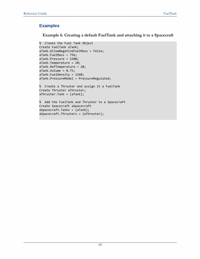
Reference Guide FuelTank
68
Examples
Example 6. Creating a default FuelTank and attaching it to a Spacecraft
% Create the Fuel Tank ObjectCreate FuelTank aTank;aTank.AllowNegativeFuelMass = false;aTank.FuelMass = 756;aTank.Pressure = 1500;aTank.Temperature = 20;aTank.RefTemperature = 20;aTank.Volume = 0.75;aTank.FuelDensity = 1260;aTank.PressureModel = PressureRegulated;
% Create a Thruster and assign it a FuelTankCreate Thruster aThruster;aThruster.Tank = {aTank};
% Add the FuelTank and Thruster to a SpacecraftCreate Spacecraft aSpacecraftaSpacecraft.Tanks = {aTank};aSpacecraft.Thrusters = {aThruster};
Reference Guide GMATFunction
69
GMATFunctionUnder Construction.
Synopsis
Under Construction.
Description
Under Construction.
Fields
Field Name Description....Type Fill This In.Default Fill This In.Limits Fill This In.Units Fill This In.
Examples
Example 7. Example Script
%
Reference Guide GroundStation
70
GroundStationUnder Construction.
Synopsis
Under Construction.
Description
Under Construction.
Fields
Field Name Description....Type Fill This In.Default Fill This In.Limits Fill This In.Units Fill This In.
Examples
Example 8. Example Script
%
Reference Guide GroundTrackPlot
71
GroundTrackPlotA GroundTrack Plot.
Synopsis
Create GroundTrackPlot namename.field = value
Description
A GroundTrackPlot is a graphical display of the locus of subsatellite latitude and longitude points.The GroundTrackPlot in GMAT allows you to view a spacecraft's subsatellite point as illustrated bya spacecraft icon and the label for the spacecraft. Similarly, GroundStation locations are indicatedwith a ground station icon and label. The GroundTrackPlot object can display the ground trackfor multiple spacecraft simultaneously and can animate the ground track evolution after a GMATrun is complete. Like other graphical dispaly objects in GMAT, you can control how data is writtento a ground track plot in iterative processes.
Fields
Fields Associated with Plot Options
DataCollectFrequency The DataCollectFrequency field allows you to select a sub-set of the ephemeris data for drawing to a GroundTrackPlot.It is often inefficient to draw every ephemeris point associatedwith a trajectory and drawing a subset of the data provides asmooth groundtrack plot with faster execution times. The Dat-aCollectFrequency is an integer that represents how manyephemeris points to skip between plotted data points in a Ground-TrackPlot. If DataCollectFrequency is set to 10, then datais collected every 10 integration steps.Default 1Limits Integer ≥ 1Units Integration Steps
UpdatePlotFrequency The UpdatePlotFrequency field allows you to specify the num-ber of ephemiris data points to collect before updating a Ground-TrackPlot with new latitude and longitude data. Data is collectedevery N propagation steps where N is defined by DataCollectFre-quency. After M points are collected, where M is defined by Up-datePlotFrequency, the GroundTrackPlot is updated with new da-ta. For example, if UpdatePlotFrequency is set to 10 and DataCol-lectFrequency is set to 2, then the plot is updated with new dataevery 20 (10*2) integration steps.Default 50Limits Integer ≥ 1Units Integration Steps
NumPointsToRedraw When NumPointsToRedraw is set to zero, all collected ephemerispoints are drawn. When NumPointsToRedraw is set to a positive
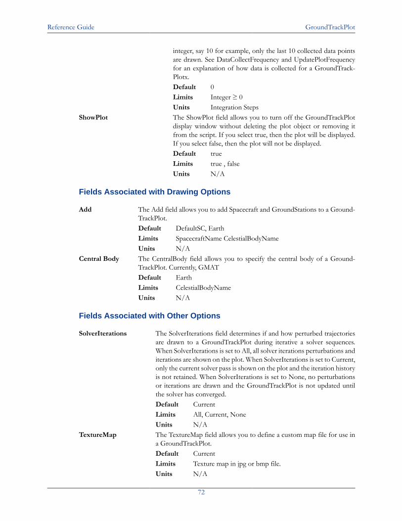
Reference Guide GroundTrackPlot
72
integer, say 10 for example, only the last 10 collected data pointsare drawn. See DataCollectFrequency and UpdatePlotFrequencyfor an explanation of how data is collected for a GroundTrack-Plotx.Default 0Limits Integer ≥ 0Units Integration Steps
ShowPlot The ShowPlot field allows you to turn off the GroundTrackPlotdisplay window without deleting the plot object or removing itfrom the script. If you select true, then the plot will be displayed.If you select false, then the plot will not be displayed.Default trueLimits true , falseUnits N/A
Fields Associated with Drawing Options
Add The Add field allows you to add Spacecraft and GroundStations to a Ground-TrackPlot.Default DefaultSC, EarthLimits SpacecraftName CelestialBodyNameUnits N/A
Central Body The CentralBody field allows you to specify the central body of a Ground-TrackPlot. Currently, GMATDefault EarthLimits CelestialBodyNameUnits N/A
Fields Associated with Other Options
SolverIterations The SolverIterations field determines if and how perturbed trajectoriesare drawn to a GroundTrackPlot during iterative a solver sequences.When SolverIterations is set to All, all solver iterations perturbations anditerations are shown on the plot. When SolverIterations is set to Current,only the current solver pass is shown on the plot and the iteration historyis not retained. When SolverIterations is set to None, no perturbationsor iterations are drawn and the GroundTrackPlot is not updated untilthe solver has converged.Default CurrentLimits All, Current, NoneUnits N/A
TextureMap The TextureMap field allows you to define a custom map file for use ina GroundTrackPlot.Default CurrentLimits Texture map in jpg or bmp file.Units N/A
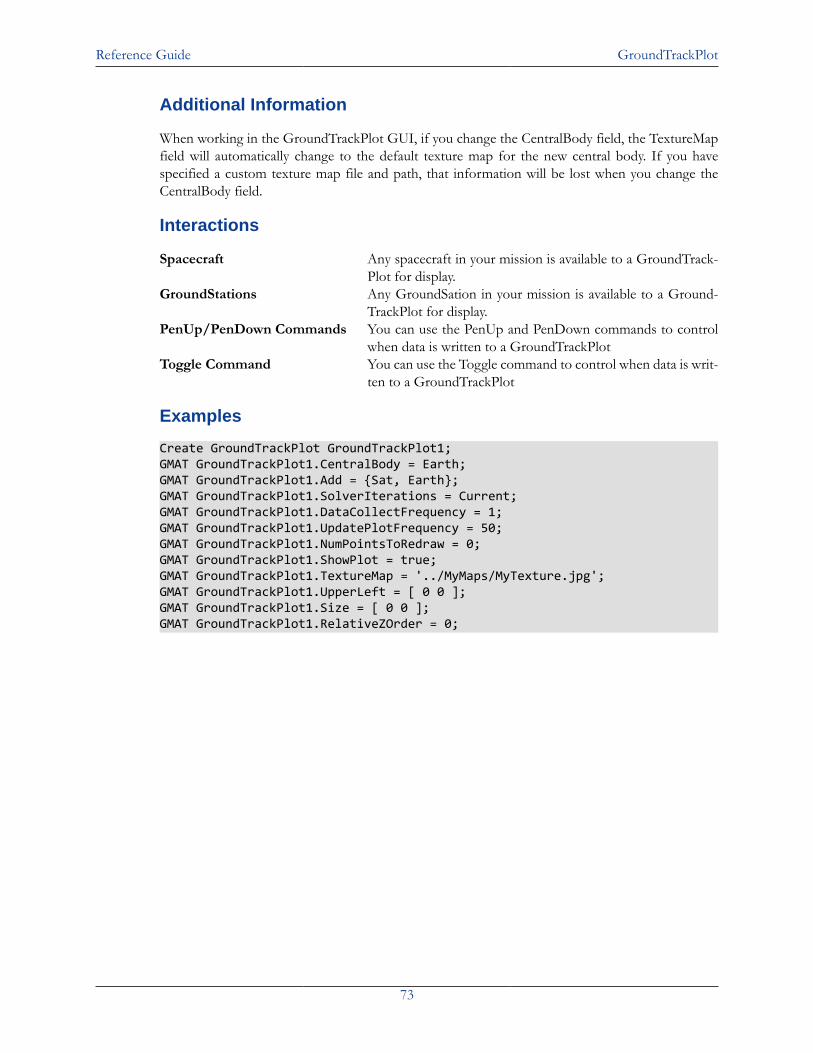
Reference Guide GroundTrackPlot
73
Additional Information
When working in the GroundTrackPlot GUI, if you change the CentralBody field, the TextureMapfield will automatically change to the default texture map for the new central body. If you havespecified a custom texture map file and path, that information will be lost when you change theCentralBody field.
Interactions
Spacecraft Any spacecraft in your mission is available to a GroundTrack-Plot for display.
GroundStations Any GroundSation in your mission is available to a Ground-TrackPlot for display.
PenUp/PenDown Commands You can use the PenUp and PenDown commands to controlwhen data is written to a GroundTrackPlot
Toggle Command You can use the Toggle command to control when data is writ-ten to a GroundTrackPlot
Examples
Create GroundTrackPlot GroundTrackPlot1;GMAT GroundTrackPlot1.CentralBody = Earth;GMAT GroundTrackPlot1.Add = {Sat, Earth};GMAT GroundTrackPlot1.SolverIterations = Current;GMAT GroundTrackPlot1.DataCollectFrequency = 1;GMAT GroundTrackPlot1.UpdatePlotFrequency = 50;GMAT GroundTrackPlot1.NumPointsToRedraw = 0;GMAT GroundTrackPlot1.ShowPlot = true;GMAT GroundTrackPlot1.TextureMap = '../MyMaps/MyTexture.jpg';GMAT GroundTrackPlot1.UpperLeft = [ 0 0 ];GMAT GroundTrackPlot1.Size = [ 0 0 ];GMAT GroundTrackPlot1.RelativeZOrder = 0;
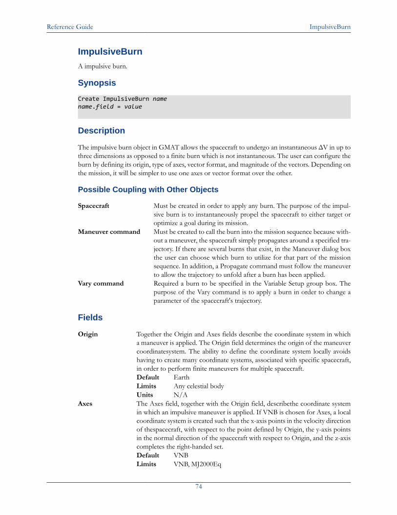
Reference Guide ImpulsiveBurn
74
ImpulsiveBurnA impulsive burn.
Synopsis
Create ImpulsiveBurn namename.field = value
Description
The impulsive burn object in GMAT allows the spacecraft to undergo an instantaneous ΔV in up tothree dimensions as opposed to a finite burn which is not instantaneous. The user can configure theburn by defining its origin, type of axes, vector format, and magnitude of the vectors. Depending onthe mission, it will be simpler to use one axes or vector format over the other.
Possible Coupling with Other Objects
Spacecraft Must be created in order to apply any burn. The purpose of the impul-sive burn is to instantaneously propel the spacecraft to either target oroptimize a goal during its mission.
Maneuver command Must be created to call the burn into the mission sequence because with-out a maneuver, the spacecraft simply propagates around a specified tra-jectory. If there are several burns that exist, in the Maneuver dialog boxthe user can choose which burn to utilize for that part of the missionsequence. In addition, a Propagate command must follow the maneuverto allow the trajectory to unfold after a burn has been applied.
Vary command Required a burn to be specified in the Variable Setup group box. Thepurpose of the Vary command is to apply a burn in order to change aparameter of the spacecraft's trajectory.
Fields
Origin Together the Origin and Axes fields describe the coordinate system in whicha maneuver is applied. The Origin field determines the origin of the maneuvercoordinatesystem. The ability to define the coordinate system locally avoidshaving to create many coordinate systems, associated with specific spacecraft,in order to perform finite maneuvers for multiple spacecraft.Default EarthLimits Any celestial bodyUnits N/A
Axes The Axes field, together with the Origin field, describethe coordinate systemin which an impulsive maneuver is applied. If VNB is chosen for Axes, a localcoordinate system is created such that the x-axis points in the velocity directionof thespacecraft, with respect to the point defined by Origin, the y-axis pointsin the normal direction of the spacecraft with respect to Origin, and the z-axiscompletes the right-handed set.Default VNBLimits VNB, MJ2000Eq
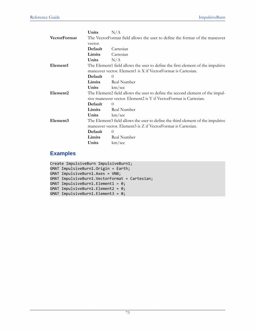
Reference Guide ImpulsiveBurn
75
Units N/AVectorFormat The VectorFormat field allows the user to define the format of the maneuver
vector.Default CartesianLimits CartesianUnits N/A
Element1 The Element1 field allows the user to define the first element of the impulsivemaneuver vector. Element1 is X if VectorFormat is Cartesian.Default 0Limits Real NumberUnits km/sec
Element2 The Element2 field allows the user to define the second element of the impul-sive maneuver vector. Element2 is Y if VectorFormat is Cartesian.Default 0Limits Real NumberUnits km/sec
Element3 The Element3 field allows the user to define the third element of the impulsivemaneuver vector. Element3 is Z if VectorFormat is Cartesian.Default 0Limits Real NumberUnits km/sec
Examples
Create ImpulsiveBurn ImpulsiveBurn1;GMAT ImpulsiveBurn1.Origin = Earth;GMAT ImpulsiveBurn1.Axes = VNB;GMAT ImpulsiveBurn1.VectorFormat = Cartesian;GMAT ImpulsiveBurn1.Element1 = 0;GMAT ImpulsiveBurn1.Element2 = 0;GMAT ImpulsiveBurn1.Element3 = 0;
Reference Guide LibrationPoint
76
LibrationPointA libration point.
Synopsis
Create LibrationPoint namename.field = value
Description
A Libration point, also called a Lagrange point, is a point of equilibrium in the restricted three-bodyproblem.
Fields
Primary The Primary field allows you to define the body treated as the primary in the calcu-lation of the libration point location. (See Math. Spec for more details).Default SunLimits Sun, Mercury, Venus, Earth, Luna, Mars, Jupiter, Saturn, Uranus, Nep-
tune, Pluto, or any Barycenter. ( The Primary and Secondary bodiescannot be the same )
Units N/ASecondary The Secondary field allows you to define the body treated as the secondary in the
calculation of the libration point location.Default EarthLimits Sun, Mercury, Venus, Earth, Luna, Mars, Jupiter, Saturn, Uranus, Nep-
tune, Pluto, or any Barycenter. ( The Primary and Secondary bodiescannot be the same )
Units N/APoint The Point field specifies which libration point the object corresponds to.
Default L1Limits L1, L2, L3, L4, L5Units N/A
Examples
Script Syntax
Create Libration Point;.Primary = ;.Secondary = ;.Point = <'L1', 'L2', 'L3', 'L4', 'L5'>
Sample Script
Create LibrationPoint Libration1;GMAT Libration1.Primary = Sun;GMAT Libration1.Secondary = Earth;

Reference Guide LibrationPoint
77
GMAT Libration1.Point = 'L1';
Reference Guide MATLABFunction
78
MATLABFunctionUnder Construction.
Synopsis
Under Construction.
Description
Under Construction.
Fields
Field Name Description....Type Fill This In.Default Fill This In.Limits Fill This In.Units Fill This In.
Examples
Example 9. Example Script
%
Reference Guide OrbitView
79
OrbitViewA 3D graphics view
Synopsis
Create OrbitView namename.field = value
Description
Without OrbitView plots, you would have no way of visualizing your spacecraft as it traveled alongits trajectory. OrbitView plots also have a multitude of options that allow you to customize yourview of the spacecraft. This makes these types of plots very useful and in most cases necessary tousing GMAT.
Fields
Fields Associated with Plot Options
DataCollectFrequency The DataCollectFrequency field allows the user to define how da-ta is collected for plotting. It is often inefficient to draw everyephemeris point associated with a trajectory. Often, drawing asmaller subset of the data still results in smooth trajectory plots,while executing more quickly. The DataCollectFrequency is an in-teger that represents how often to collect data and store for plot-ting. If DataCollectFrequency is set to 10, then Data is collectedevery 10 integration steps.Default 1Limits Integer ≥ 1Units Integration Steps
UpdatePlotFrequency The UpdatePlotFrequency field allows the user to specify how of-ten to update an OrbitView plot is updated with new data col-lected during the process of propagating spacecraft and runninga mission. Data is collected for a plot according the value definedby DataCollectFrequency. An OrbitView plot is updated with thenew data, according to the value set in UpdatePlotFrequency. IfUpdatePlotFrequency is set to 10 and DataCollectFrequency is setto 2, then the plot is updated with new data every 20 (10*2) inte-gration steps.Default 50Limits Integer ≥ 1Units Integration Steps
NumPointsToRedraw When NumPointsToRedraw is set to zero, all ephemeris points aredrawn. When NumPointsToRedraw is set to a positive integer, say10 for example, only the last 10 collected data points are drawn.See DataCollectFrequency for explanation of how data is collectedfor an OrbitView plot.Default 0Limits Integer ≥ 0
Reference Guide OrbitView
80
Units Integration StepsShowPlot The ShowPlot field allows the user to turn off a plot for a partic-
ular run, without deleting the plot object, or removing it from thescript. If you select true, then the plot will be shown. If you selectfalse, then the plot will not be shown.Default trueLimits true , falseUnits N/A
Fields Associated with Viewed Objects
Add The Add subfield adds a spacecraft,celestial body, libration point,or barycenter to a plot.When creating a plot the Earth is added as a default body and may be removed by usingthe Remove command. The user can add a spacecraft, celestial body, libration point, orbarycenter to a plot by using the name used to create the object. The GUI's Selectedfield is the equivalent of the script's Add field. In the event of no Add command orno objects in the Selected field, GMAT should run without the OrbitView plot and awarning message displayed in the message window. The following warning message issufficient: OrbitView plot will be turned off. No object has been selected for plotting.Default DefaultSC, EarthLimits SpacecraftName CelestialBodyName LibrationPointName Barycenter-
NameUnits N/A
Remove The Remove subfield removes a spacecraft,celestial body, libration point, or barycenterfrom a plot. The user can remove any object that has been added to a plot by using thename used to add the object.Default No DefaultLimits Any object included in the Add listUnits N/A
Fields Associated with Drawing Options
WireFrame When the WireFrame field is set to On, celestial bodies are drawn using awireframe model. When the WireFrame field is set to Off, then celestialbodies are drawn using a full map.Default OffLimits On , OffUnits N/A
EclipticPlane The EclipticPlane field allows the user to tell GMAT to draw a grid rep-resenting the ecliptic plane in an OrbitView plot. Note, the ecliptic planecan currently only be drawn for plots whose coordinate system uses theMJ2000Eq axis system.Default OffLimits On , Off Note: Only allowed for OrbitView plots with Co-
ordinate Systems that use the MJ2000Eq axis systemUnits N/A
XYPlane The XYPlane flag allows the user to tell GMAT to draw a grid repre-senting the XY-plane of the coordinate system selected under the Coor-dinateSystem field of the OrbitView plot.Default On
Reference Guide OrbitView
81
Limits On , OffUnits N/A
Axes The Axis flag allows the user to tell GMAT to draw the Cartesian axissystem associated with the coordinate system selected under the Coor-dinateSystem field of an OrbitView plot.Default OnLimits On , OffUnits N/A
Grid The Grid flag allows the user to tell GMAT to draw a grid representingthe longitude and latitude lines celestial bodies added to an OrbitViewplot.Default OnLimits On , OffUnits N/A
EarthSunLines The EarthSunLines allows the user to tell GMAT to draw a line thatstarts at the center of Earth and points towards the Sun.Default OnLimits On , OffUnits N/A
SolverIterations The SolverIterations field determines whether or not perturbed trajec-tories are plotted during a solver (Targeter, Optimize) sequence. WhenSolverIterations is set to On, solver iterations are shown on the plot.When SolverIterations is Off, the solver iterations are not shown on theplot.Default OffLimits On , OffUnits N/A
Fields Associated with View Definition
CoordinateSystem The CoordinateSystem field on an OrbitView plot allows the user toselect which coordinate system to use to draw the plot data. A coor-dinate system is defined as an origin and an axis system, and the Co-ordinateSystem field allows the user to determine the origin and axissystem of an OrbitView plot. See the CoordinateSystem object fieldsfor information of defining different types of coordinate systems.Default EarthMJ2000EqLimits Any default or user defined coordinate systemUnits N/A
ViewPointReference The ViewPointReference field is an optional field that allows the userto change the reference point from which ViewPointVector is mea-sured. ViewPointReference} defaults to the origin of the coordinatesystem for the plot. A ViewPointReference can be any spacecraft, ce-lestial body, libration point, or barycenter.Default EarthLimits SpacecraftName, CelestialBodyName, LibrationPoint-
Name, BarycenterName, or a 3-vector of numerical val-ues
Units N/A
Reference Guide OrbitView
82
ViewPointVector The product of ViewScaleFactor and ViewPointVector field deter-mines the view point location with respect to ViewPointReference.ViewPointVector can be a vector, or any of the following objects:spacecraft,celestial body, libration point,or barycenter. The locationof the Viewpoint in three-space is defined as the vector addition ofViewPointReference, and the vector defined by product of ViewS-caleFactor and ViewPointVector in the coordinate system chosen bythe user.Default [0 0 30000]Limits SpacecraftName, CelestialBodyName, LibrationPoint-
Name, BarycenterName, or a 3-vector of numerical val-ues
Units km or N/AViewScaleFactor The ViewScaleFactor field scales ViewPointVector before adding it
to ViewPointReference. The ViewScaleFactor allows the user to backaway from an object to fit in the field of view.Default 1Limits Real Number ≥ 0Units N/A
ViewDirection The ViewDirection field allows the user to select the direction ofview in an OrbitView plot. The user can specify the view directionby choosing an object to point at such as a spacecraft,celestial body,libration point,or barycenter. Alternatively, the user can specify a vec-tor of the form [x y z]. If the user specification of ViewDirection,ViewPointReference, and ViewPointVector, results in a zero vector,GMAT uses [0 0 10000] for ViewDirection.Default EarthLimits SpacecraftName, CelestialBodyName, LibrationPoint-
Name, BarycenterName, or a 3-vector of numerical val-ues
Units km or N/A
Fields Associated with View Options
UseInitialView The UseInitialView field allows the user to control the view of an OrbitViewplot between multiple runs of a mission sequence. The first time a specificOrbitView plot is created, GMAT will automatically use the view as definedby the fields associated with View Definition, View Up Direction, and Fieldof View. However, if the user changes the view using the mouse, GMATwill retain this view upon rerunning the mission if UseInitialView is set tofalse. If UseInitialView is set to true, the view for an OrbitView plot will bereturned to the view defined by the initial settings.Default OnLimits On , OffUnits N/A
Fields Associated with View Up Definition
ViewUpCoordinate System The ViewUpCoordinateSystem and ViewUpAxis fields areused to determine which direction appears as up in an Or-
Reference Guide OrbitView
83
bitView plot and together with the fields associated the theView Direction, uniquely define the view. The fields associat-ed with the View Definition allow the user to define the pointof view in 3-space, and the direction of the line of sight. How-ever, this information alone is not enough to uniquely definethe view. We also must provide how the view is oriented aboutthe line of sight. This is accomplished by defining what di-rection should appear as the up direction in the plot and isconfigured using the ViewUpCoordinateSystem field and theViewUpAxis field. The ViewUpCoordinateSystem allows theuser to select a coordinate system to define the up direction.Most of the time this system will be the same as the coordi-nate system chosen under the CoordinateSystem field.Default EarthMJ2000EqLimits Any default or user defined coordinate systemUnits N/A
ViewUpAxis The ViewUpAxis allows the user to define which axis of theViewUpCoordinateSystem that will appear as the up directionin an OrbitView plot. See the comments under ViewUpCo-ordinateSystem for more details of fields used to determinethe up direction in an OrbitView plot.Default ZLimits X , -X , Y , -Y , Z , -ZUnits N/A
Interactions
Spacecraft Any spacecraft in your mission is available to the OrbitView plot fordisplay
Solar System The Sun and all of the Planets may be plotted or referenced in theOrbitView plot
If you add any Barrycenters or Libration Points, they will also be avail-able for plotting and reference
Coordinate Systems Both View Definition and View Up Definition may use the three de-fault or user added coordinate systems
Examples
Create OrbitView DefaultOpenGL;GMAT DefaultOpenGL.SolverIterations = Current;GMAT DefaultOpenGL.Add = {DefaultSC, Earth};GMAT DefaultOpenGL.OrbitColor = [ 255 32768 ];GMAT DefaultOpenGL.TargetColor = [ 8421440 0 ];GMAT DefaultOpenGL.CoordinateSystem = EarthMJ2000Eq;GMAT DefaultOpenGL.ViewPointReference = Earth;GMAT DefaultOpenGL.ViewPointVector = [ 0 0 30000 ];GMAT DefaultOpenGL.ViewDirection = Earth;GMAT DefaultOpenGL.ViewScaleFactor = 1;GMAT DefaultOpenGL.ViewUpCoordinateSystem = EarthMJ2000Eq;GMAT DefaultOpenGL.ViewUpAxis = Z;
Reference Guide OrbitView
84
GMAT DefaultOpenGL.CelestialPlane = Off;GMAT DefaultOpenGL.XYPlane = On;GMAT DefaultOpenGL.WireFrame = Off;GMAT DefaultOpenGL.Axes = On;GMAT DefaultOpenGL.Grid = Off;GMAT DefaultOpenGL.SunLine = Off;GMAT DefaultOpenGL.UseInitialView = On;GMAT DefaultOpenGL.DataCollectFrequency = 1;GMAT DefaultOpenGL.UpdatePlotFrequency = 50;GMAT DefaultOpenGL.NumPointsToRedraw = 0;GMAT DefaultOpenGL.ShowPlot = true;
Reference Guide Propagator
85
Propagator
A propagator.
Synopsis
Create Propagator namename.field = value
Description
In GMAT, a Propagator is a combination of an integrator and a force model. Hence, a Propagatorcontains a physical model of the space environment that is used to model the motion of a spacecraftas it moves forwards or backwards in time (VOP formulation is not currently supported). You con-figure a Propagator by selecting among different numerical integrators and environment models tocreate a Propagator appropriate to the flight regime of your spacecraft during its mission. GMATsupports numerous numerical integrators as well as Force Models like point mass and non-sphericalgravity, atmospheric drag (Earth), and solar radiation pressure.
To propagate spacecraft in GMAT, you first create and configure a Propagator object in the script orin the Resource Tree. Then, in the mission sequence, you create a Propagate command, the topic ofanother section, and select among previously existing Propagators and Spacecraft. Hence, a Propa-gator is different from a Propagate command: A Propagator is a resource and is found in the GUIunder the resource tree, and a Propagate Event is configured under the Mission Tree and is how youinstruct GMAT to propagate spacecraft.
Interfaces
The Propagator dialog box is illustrated below and contains two group boxes: the Integrator groupand the Force Model group. This section discusses the items in each group on the Propagate Panel.It will present how to configure a propagator and discuss all possible user settable fields in detail.
Integrator Group
The Integrator group allows you to select and configure a numerical integrator appropriate to yourapplication. You select the type of numerical integrator in the -+Type+- pull-down menu. Afterselecting the integrator type, the fields below the -+Type+- pull-down menu dynamically configureto allow you to set relevant parameters for the selected integrator type. All integrators except forAdams-Bashforth-Moulton (ABM) are configured using the same fields. The ABM integrator hasthe following additional fields: -+MinIntegrationerror+- and -+NomIntegrationerror+-.
Force Model Group
The Force Model group allows you to configure a force model appropriate to the flight regimeof your application. The central body of propagation and error control method are also definedhere. On a Propagator, GMAT classifies all celestial bodies into two mutually exclusive categories:Primary Bodies, and Point Masses. Primary bodies can have a complex force model that includes non-spherical gravity, drag, and magnetic field. Point mass bodies only have a point-mass gravitationalforce.
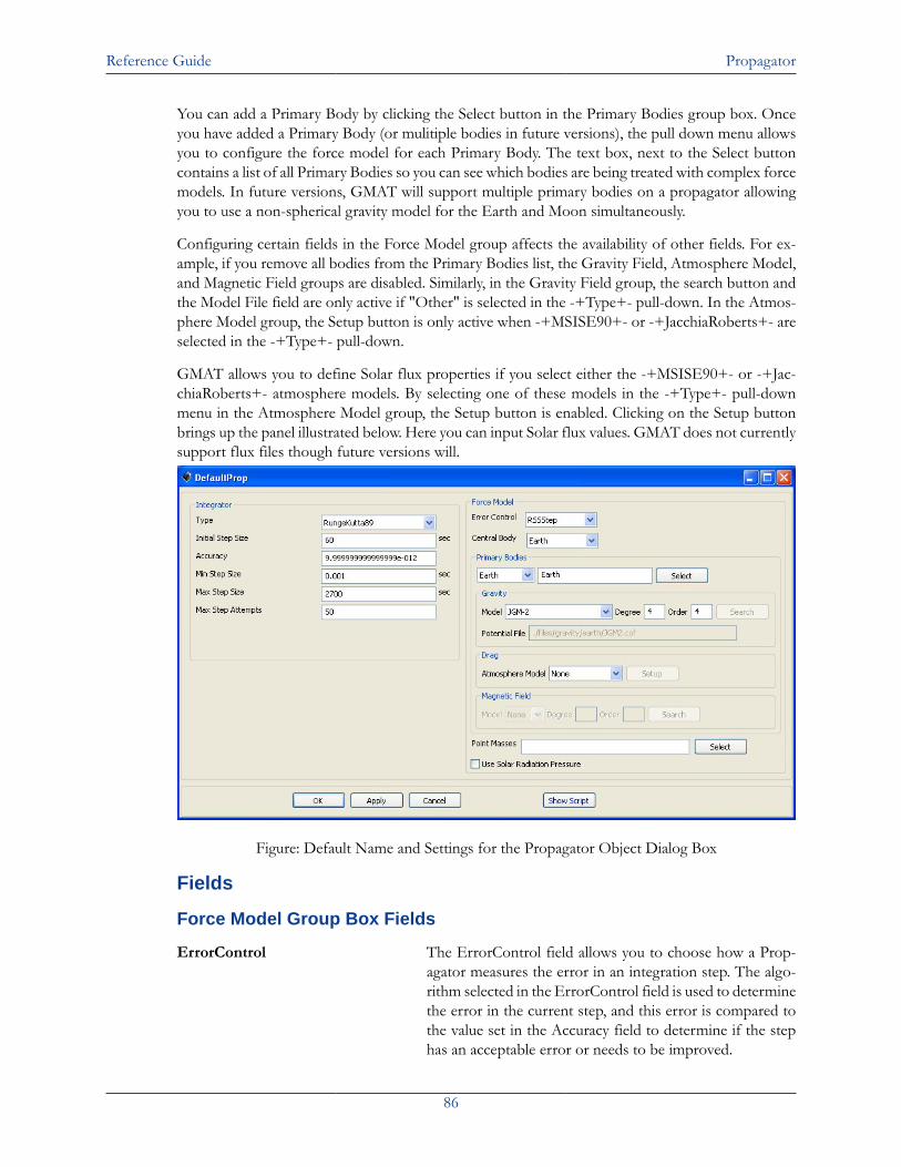
Reference Guide Propagator
86
You can add a Primary Body by clicking the Select button in the Primary Bodies group box. Onceyou have added a Primary Body (or mulitiple bodies in future versions), the pull down menu allowsyou to configure the force model for each Primary Body. The text box, next to the Select buttoncontains a list of all Primary Bodies so you can see which bodies are being treated with complex forcemodels. In future versions, GMAT will support multiple primary bodies on a propagator allowingyou to use a non-spherical gravity model for the Earth and Moon simultaneously.
Configuring certain fields in the Force Model group affects the availability of other fields. For ex-ample, if you remove all bodies from the Primary Bodies list, the Gravity Field, Atmosphere Model,and Magnetic Field groups are disabled. Similarly, in the Gravity Field group, the search button andthe Model File field are only active if "Other" is selected in the -+Type+- pull-down. In the Atmos-phere Model group, the Setup button is only active when -+MSISE90+- or -+JacchiaRoberts+- areselected in the -+Type+- pull-down.
GMAT allows you to define Solar flux properties if you select either the -+MSISE90+- or -+Jac-chiaRoberts+- atmosphere models. By selecting one of these models in the -+Type+- pull-downmenu in the Atmosphere Model group, the Setup button is enabled. Clicking on the Setup buttonbrings up the panel illustrated below. Here you can input Solar flux values. GMAT does not currentlysupport flux files though future versions will.
Figure: Default Name and Settings for the Propagator Object Dialog Box
Fields
Force Model Group Box Fields
ErrorControl The ErrorControl field allows you to choose how a Prop-agator measures the error in an integration step. The algo-rithm selected in the ErrorControl field is used to determinethe error in the current step, and this error is compared tothe value set in the Accuracy field to determine if the stephas an acceptable error or needs to be improved.
Reference Guide Propagator
87
All error measurements are relative error, however, the ref-erence for the relative error changes depending upon theselection of ErrorControl. RSSStep is the Root Sum Square(RSS) relative error measured with respect to the currentstep. RSSState is the (RSS) relative error measured with re-spect to the current state. LargestStep is the state vectorcomponent with the largest relative error measured with re-spect to the current step. LargestState is the state vectorcomponent with the largest relative error measured with re-spect to the current state. For a more detailed discussion seethe GMAT Mathematical Specification. Units: N/A.Default RSSStepLimits RSSStep, RSSState, LargestState, LargestStep
CentralBody The CentralBody field allows the user to select the originfor the propagation. All propagation occurs in the FK5 ax-es system, about the CentralBody chosen by the user. TheCentralBody must be a gravitational body and so cannot bea LibrationPoint or other special point.Default EarthLimits Sun, Mercury, Venus, Earth, Luna, Mars,
Jupiter, Saturn, Uranus, Neptune, PlutoUnits N/A
PrimaryBodies The PrimaryBodies field is a list of all celestial bodies that areto be modelled with a force model more complex than pointmass gravity. Lists are surrounded by curly braces. For eachPrimaryBody, the user can choose a drag, magnetic field, andaspherical gravity model. There is a coupling between thePrimaryBodies filed and the PointMasses field. A primarybody can be any planet or moon not included in the Point-Masses field.Default EarthLimits Sun, Mercury, Venus, Earth, Luna, Mars,
Jupiter, Saturn, Uranus, Neptune, PlutoUnits N/A
Gravity.PrimaryBody.PotentialFile This field allows the user to define the source for the non-spherical gravity coefficients for a primary body. If a gravi-ty file is located in the Primary Body's potential path as de-fined in the startup file, you only need to specify the mod-el name and not the entire path. For example, if the JGM2coefficients file is contained in the directory defined in thestartup file by the line EARTH\_POT\_PATH, then youonly need to specify the model name JGM2. If the model isnot contained in the body's potential path, you must supplythe entire path as well as the file name. If GMAT does notsuccessfully find the file requested, it uses the default grav-ity model as defined in the startup file. From the GUI, onlymodels for Earth appear if Earth is the active primary body.This is to avoid allowing the user to select a lunar potential
Reference Guide Propagator
88
model for the Earth. If the Other option is selected the userhas the ability of selecting a gravity model file on their localcomputer.Default JGM2Limits CentralBody-based models, Other. See Com-
mentsUnits N/A
Gravity.PrimaryBody.Degree This field allows the user to select the the degree, or num-ber of zonal terms, in the non-spherical gravity model. Ex.Gravity.Earth.Degree = 2 tells GMAT to use only the J2zonal term for the Earth. The value for Degree must be lessthan the maximum degree specified by the Model.Default 4Limits Integer >= 0 and < the maximum specified by
the model, Order <= DegreeUnits N/A
Gravity.PrimaryBody.Order This field allows the user to select the the order, or numberof tesseral terms, in the non-spherical gravity model. Ex.Gravity.Earth.Order = 2 tells GMAT to use 2 tesseral terms.Note: Order must be greater than or equal to Degree.Default 4Limits Integer >= 0 and < the maximum specified by
the model, Order <= DegreeUnits N/A
Drag The Drag field allows a user to specify a drag model. Cur-rently, only one drag model can be chosen for a particularpropagator and only Earth models are available.Default N/ALimits None, JacchiaRoberts, MSISE90, ExponentialUnits N/A. Note: This field will be deprecated in
future versions of GMAT. Currently, the Dragfield and the Drag.AtmosphereModel fieldmust be set to the same value.
Drag.AtmosphereModel The Drag.AtmosphereModel field allows a user to specifya drag model. Currently, only one drag model can be cho-sen for a particular propagator and only Earth models areavailable.Default NoneLimits None, JacchiaRoberts, MSISE90, ExponentialUnits N/A
Drag.F107 The Drag.F107 field allows you to set the F10.7 solar fluxvalue used in computing atmospheric density. F10.7 is thesolar radiation at a wavelength of 10.7 cm.Default 150Limits Real Number >= 0Units W/m2/Hz
Drag.F107A The Drag.F107A field allows you to set the average F10.7value. F10.7 is the average of F10.7 over one month.Default 150
Reference Guide Propagator
89
Limits Real Number >= 0Units W/m2/Hz
Drag.MagneticIndex The Drag.MagneticIndex index field allows you to set thekp value for use in atmospheric density calculations. kp is aplanetary 3-hour-average, geomagnetic index that measuresmagnetic effects of solar radiation.Default 3Limits 0 <= Real Number <= 9Units N/A
PointMasses A PointMass is a planet or moon that is modelled by a pointsource located at its center of gravity. A PointMass body canbe any planet or moon not included in the PrimaryBodiesfield.Default NoneLimits Sun, Mercury, Venus, Earth, Luna, Mars,
Jupiter, Saturn, Uranus, Neptune, PlutoUnits N/A
SRP The SRP field allows the user to include the force due tosolar radiation pressure in the total sum of forces.Default OffLimits On, OffUnits N/A
Integrator Group Box Fields
Type The Type field is used to set the type of numerical integrator.Default RungeKutta89Limits RungeKutta89, RungeKutta68, RungeKutta56, PrinceDor-
mand45, PrinceDormand78, BulirschStoer, AdamsBash-forthMoulton
InitialStepSize The InitialStepSize is the size of the first attempted step by the integrator.If the step defined by InitialStepSize does not satisfy Accuracy, the inte-grator adapts the step according an algorithm defined in the mathemati-cal specifications document to find an acceptable first step that meets theuser's requested.Default 60 (sec)Limits Real NumberUnits seconds
Accuracy The Accuracy field is used to set the desired accuracy for an integrationstep. When you set a value for Accuracy, GMAT uses the method selectedin ErrorControl field on the Force Model, to determine a metric of the ac-curacy. For each step, the integrator ensures that the accuracy, as calculatedusing the method defined by ErrorControl, is less than the limit definedby Accuracy. If an integrator exceeds MaxStepAttempts trying to meet therequested accuracy, and error message is thrown and propagation stops.Default 1e-11Limits Real Number >= 0Units N/A
MinStep The MinStep field is used to set the minimum allowable step size.
Reference Guide Propagator
90
Default .001 (sec)Limits Real Number > 0, MinStep <= MaxStepUnits seconds
MaxStep The MaxStep field is used to set the maximum allowable step size.Default 2700.0 (sec)Limits Real Number > 0, MinStep <= MaxStepUnits seconds
MaxStepAttempts The MaxStepAttempts field allows the user to set the number of attemptsthe integrator takes to meet the tolerance defined by Accuracy.Default 50Limits Integer > 0Units None
Fields Associated Only with Adams-Bashforth-Moulton Integrator
MinIntegrationerror The MinIntegrationerror field is used by the ABM integrator (andother predictor-corrector integrators when implemented) as the de-sired integration error to be obtained when the step size is changed.Predictor-Corrector integrators adapt step size when the obtainedintegration error falls outside of the range of acceptable steps, asdetermined by the bounds set by the MinIntegrationerror and Ac-curacy fields. The integrator then applies an internal calculation torecompute the step size, attempting to hit the NomIntegrationerror,and restarts the integrator.Default 1.0e-13Limits Real Number > 0, MinIntegrationerror < NomInte-
grationerror < AccuracyUnits None
NomIntegrationerror The NomIntegrationerror field is used by the ABM integrator (andother predictor-corrector integrators when implemented) as the de-sired integration error to be obtained when the step size is changed.Predictor-Corrector integrators adapt step size when the obtainedintegration error falls outside of the range of acceptable steps, asdetermined by the bounds set by the MinIntegrationerror and Ac-curacy fields. The integrator then applies an internal calculation torecompute the step size, attempting to hit the NomIntegrationerror,and restarts the integrator.Default 1.0e-11Limits Real Number > 0, MinIntegrationerror , NomIntegra-
tionerror , AccuracyUnits None
Interactions
A Propagator Requires Other Objects/Commands of Type: Force Model (Script Only). (Note: Thereare slight differences in how you configure a Propagator in the script and GUI and we refer youto the script example shown in the script section for details. Effort has been made to reduce anydifference between the script and GUI.)
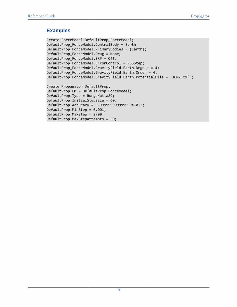
Reference Guide Propagator
91
Examples
Create ForceModel DefaultProp_ForceModel;DefaultProp_ForceModel.CentralBody = Earth;DefaultProp_ForceModel.PrimaryBodies = {Earth};DefaultProp_ForceModel.Drag = None;DefaultProp_ForceModel.SRP = Off;DefaultProp_ForceModel.ErrorControl = RSSStep;DefaultProp_ForceModel.GravityField.Earth.Degree = 4;DefaultProp_ForceModel.GravityField.Earth.Order = 4;DefaultProp_ForceModel.GravityField.Earth.PotentialFile = 'JGM2.cof';
Create Propagator DefaultProp;DefaultProp.FM = DefaultProp_ForceModel;DefaultProp.Type = RungeKutta89;DefaultProp.InitialStepSize = 60;DefaultProp.Accuracy = 9.999999999999999e-012;DefaultProp.MinStep = 0.001;DefaultProp.MaxStep = 2700;DefaultProp.MaxStepAttempts = 50;
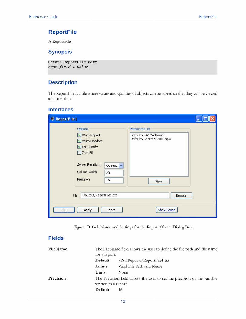
Reference Guide ReportFile
92
ReportFile
A ReportFile.
Synopsis
Create ReportFile namename.field = value
Description
The ReportFile is a file where values and qualities of objects can be stored so that they can be viewedat a later time.
Interfaces
Figure: Default Name and Settings for the Report Object Dialog Box
Fields
FileName The FileName field allows the user to define the file path and file namefor a report.Default /RunReports/ReportFile1.txtLimits Valid File Path and NameUnits None
Precision The Precision field allows the user to set the precision of the variablewritten to a report.Default 16
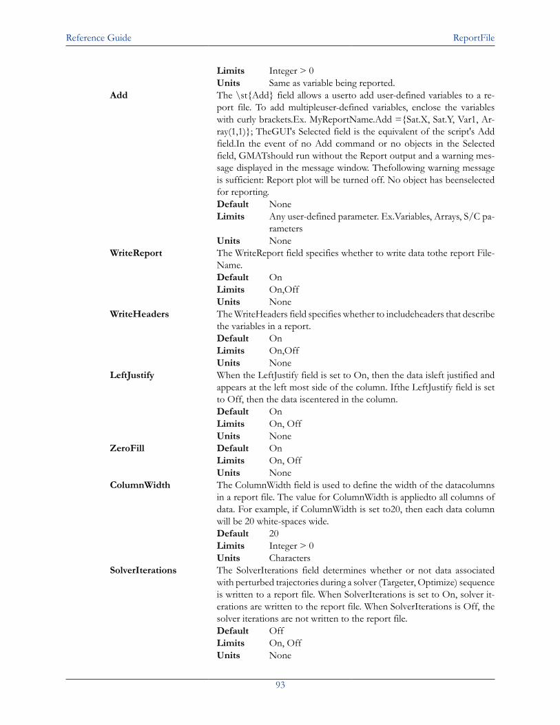
Reference Guide ReportFile
93
Limits Integer > 0Units Same as variable being reported.
Add The \st{Add} field allows a userto add user-defined variables to a re-port file. To add multipleuser-defined variables, enclose the variableswith curly brackets.Ex. MyReportName.Add ={Sat.X, Sat.Y, Var1, Ar-ray(1,1)}; TheGUI's Selected field is the equivalent of the script's Addfield.In the event of no Add command or no objects in the Selectedfield, GMATshould run without the Report output and a warning mes-sage displayed in the message window. Thefollowing warning messageis sufficient: Report plot will be turned off. No object has beenselectedfor reporting.Default NoneLimits Any user-defined parameter. Ex.Variables, Arrays, S/C pa-
rametersUnits None
WriteReport The WriteReport field specifies whether to write data tothe report File-Name.Default OnLimits On,OffUnits None
WriteHeaders The WriteHeaders field specifies whether to includeheaders that describethe variables in a report.Default OnLimits On,OffUnits None
LeftJustify When the LeftJustify field is set to On, then the data isleft justified andappears at the left most side of the column. Ifthe LeftJustify field is setto Off, then the data iscentered in the column.Default OnLimits On, OffUnits None
ZeroFill Default OnLimits On, OffUnits None
ColumnWidth The ColumnWidth field is used to define the width of the datacolumnsin a report file. The value for ColumnWidth is appliedto all columns ofdata. For example, if ColumnWidth is set to20, then each data columnwill be 20 white-spaces wide.Default 20Limits Integer > 0Units Characters
SolverIterations The SolverIterations field determines whether or not data associatedwith perturbed trajectories during a solver (Targeter, Optimize) sequenceis written to a report file. When SolverIterations is set to On, solver it-erations are written to the report file. When SolverIterations is Off, thesolver iterations are not written to the report file.Default OffLimits On, OffUnits None
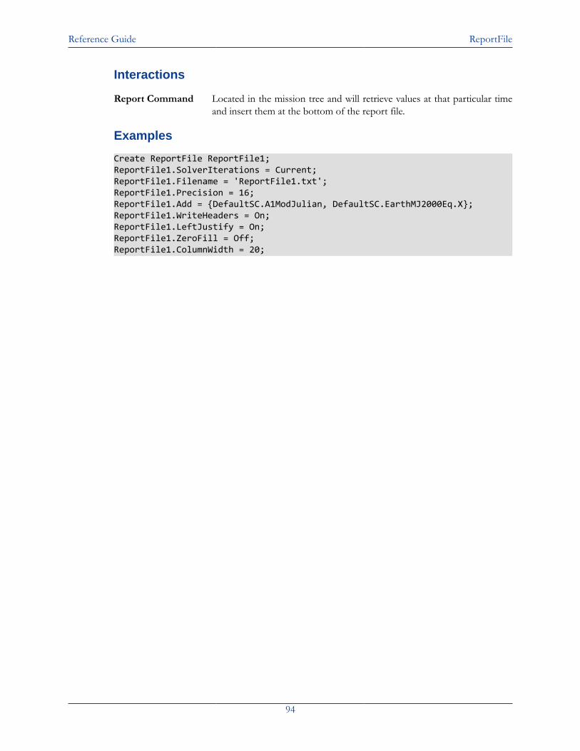
Reference Guide ReportFile
94
Interactions
Report Command Located in the mission tree and will retrieve values at that particular timeand insert them at the bottom of the report file.
Examples
Create ReportFile ReportFile1;ReportFile1.SolverIterations = Current;ReportFile1.Filename = 'ReportFile1.txt';ReportFile1.Precision = 16;ReportFile1.Add = {DefaultSC.A1ModJulian, DefaultSC.EarthMJ2000Eq.X};ReportFile1.WriteHeaders = On;ReportFile1.LeftJustify = On;ReportFile1.ZeroFill = Off;ReportFile1.ColumnWidth = 20;
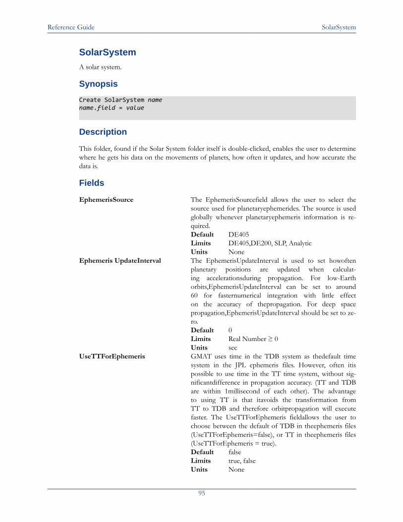
Reference Guide SolarSystem
95
SolarSystemA solar system.
Synopsis
Create SolarSystem namename.field = value
Description
This folder, found if the Solar System folder itself is double-clicked, enables the user to determinewhere he gets his data on the movements of planets, how often it updates, and how accurate thedata is.
Fields
EphemerisSource The EphemerisSourcefield allows the user to select thesource used for planetaryephemerides. The source is usedglobally whenever planetaryephemeris information is re-quired.Default DE405Limits DE405,DE200, SLP, AnalyticUnits None
Ephemeris UpdateInterval The EphemerisUpdateInterval is used to set howoftenplanetary positions are updated when calculat-ing accelerationsduring propagation. For low-Earthorbits,EphemerisUpdateInterval can be set to around60 for fasternumerical integration with little effecton the accuracy of thepropagation. For deep spacepropagation,EphemerisUpdateInterval should be set to ze-ro.Default 0Limits Real Number ≥ 0Units sec
UseTTForEphemeris GMAT uses time in the TDB system as thedefault timesystem in the JPL ephemeris files. However, often itispossible to use time in the TT time system, without sig-nificantdifference in propagation accuracy. (TT and TDBare within 1millisecond of each other). The advantageto using TT is that itavoids the transformation fromTT to TDB and therefore orbitpropagation will executefaster. The UseTTForEphemeris fieldallows the user tochoose between the default of TDB in theephemeris files(UseTTForEphemeris=false), or TT in theephemeris files(UseTTForEphemeris = true).Default falseLimits true, falseUnits None
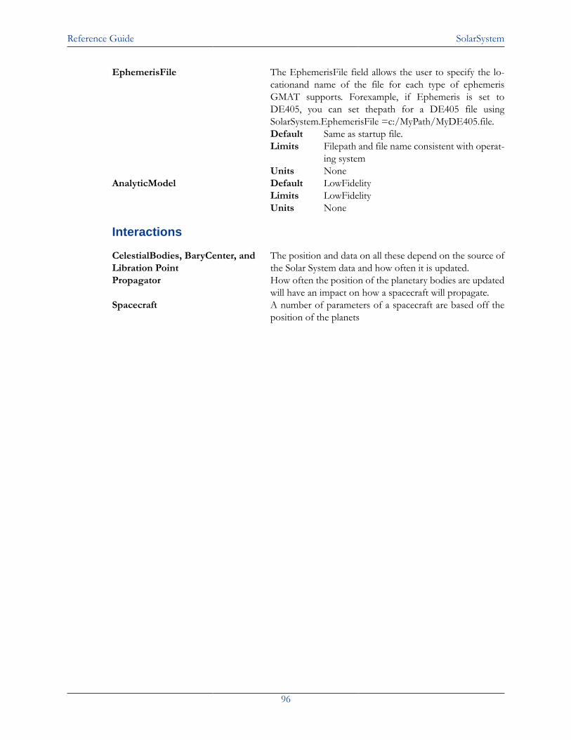
Reference Guide SolarSystem
96
EphemerisFile The EphemerisFile field allows the user to specify the lo-cationand name of the file for each type of ephemerisGMAT supports. Forexample, if Ephemeris is set toDE405, you can set thepath for a DE405 file usingSolarSystem.EphemerisFile =c:/MyPath/MyDE405.file.Default Same as startup file.Limits Filepath and file name consistent with operat-
ing systemUnits None
AnalyticModel Default LowFidelityLimits LowFidelityUnits None
Interactions
CelestialBodies, BaryCenter, andLibration Point
The position and data on all these depend on the source ofthe Solar System data and how often it is updated.
Propagator How often the position of the planetary bodies are updatedwill have an impact on how a spacecraft will propagate.
Spacecraft A number of parameters of a spacecraft are based off theposition of the planets
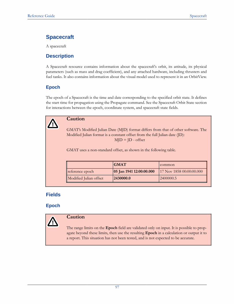
Reference Guide Spacecraft
97
Spacecraft
A spacecraft
Description
A Spacecraft resource contains information about the spacecraft's orbit, its attitude, its physicalparameters (such as mass and drag coefficient), and any attached hardware, including thrusters andfuel tanks. It also contains information about the visual model used to represent it in an OrbitView.
Epoch
The epoch of a Spacecraft is the time and date corresponding to the specified orbit state. It definesthe start time for propagation using the Propagate command. See the Spacecraft Orbit State sectionfor interactions between the epoch, coordinate system, and spacecraft state fields.
Caution
GMAT’s Modified Julian Date (MJD) format differs from that of other software. TheModified Julian format is a constant offset from the full Julian date (JD):
MJD = JD - offset
GMAT uses a non-standard offset, as shown in the following table.
GMAT common
reference epoch 05 Jan 1941 12:00:00.000 17 Nov 1858 00:00:00.000
Modified Julian offset 2430000.0 2400000.5
Fields
Epoch
Caution
The range limits on the Epoch field are validated only on input. It is possible to prop-agate beyond these limits, then use the resulting Epoch in a calculation or output it toa report. This situation has not been tested, and is not expected to be accurate.
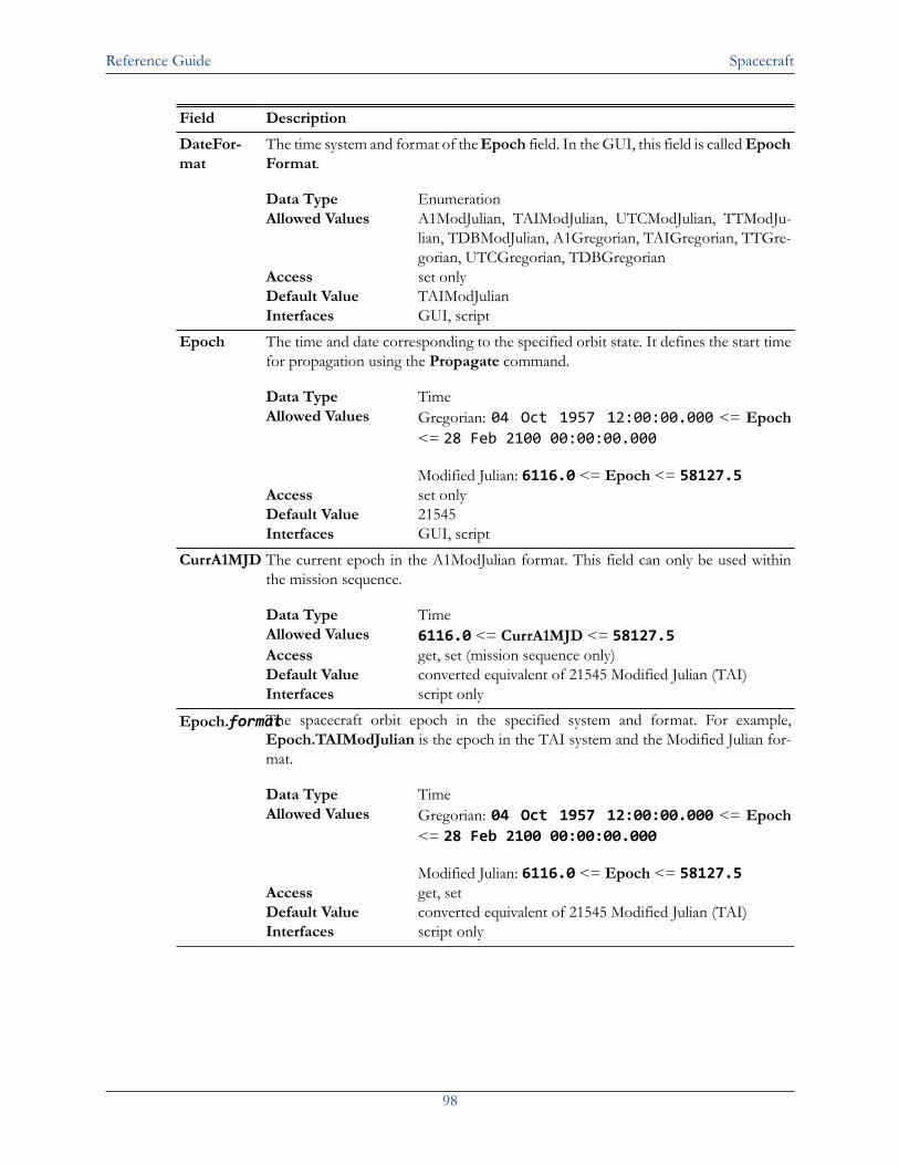
Reference Guide Spacecraft
98
Field Description
DateFor-mat
The time system and format of the Epoch field. In the GUI, this field is called EpochFormat.
Data Type EnumerationAllowed Values A1ModJulian, TAIModJulian, UTCModJulian, TTModJu-
lian, TDBModJulian, A1Gregorian, TAIGregorian, TTGre-gorian, UTCGregorian, TDBGregorian
Access set onlyDefault Value TAIModJulianInterfaces GUI, script
Epoch The time and date corresponding to the specified orbit state. It defines the start timefor propagation using the Propagate command.
Data Type TimeAllowed Values Gregorian: 04 Oct 1957 12:00:00.000 <= Epoch
<= 28 Feb 2100 00:00:00.000
Modified Julian: 6116.0 <= Epoch <= 58127.5Access set onlyDefault Value 21545Interfaces GUI, script
CurrA1MJD The current epoch in the A1ModJulian format. This field can only be used withinthe mission sequence.
Data Type TimeAllowed Values 6116.0 <= CurrA1MJD <= 58127.5Access get, set (mission sequence only)Default Value converted equivalent of 21545 Modified Julian (TAI)Interfaces script only
Epoch.formatThe spacecraft orbit epoch in the specified system and format. For example,Epoch.TAIModJulian is the epoch in the TAI system and the Modified Julian for-mat.
Data Type TimeAllowed Values Gregorian: 04 Oct 1957 12:00:00.000 <= Epoch
<= 28 Feb 2100 00:00:00.000
Modified Julian: 6116.0 <= Epoch <= 58127.5Access get, setDefault Value converted equivalent of 21545 Modified Julian (TAI)Interfaces script only
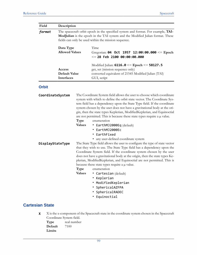
Reference Guide Spacecraft
99
Field Description
format The spacecraft orbit epoch in the specified system and format. For example, TAI-ModJulian is the epoch in the TAI system and the Modified Julian format. Thesefields can only be used within the mission sequence.
Data Type TimeAllowed Values Gregorian: 04 Oct 1957 12:00:00.000 <= Epoch
<= 28 Feb 2100 00:00:00.000
Modified Julian: 6116.0 <= Epoch <= 58127.5Access get, set (mission sequence only)Default Value converted equivalent of 21545 Modified Julian (TAI)Interfaces GUI, script
Orbit
CoordinateSystem The Coordinate System field allows the user to choose which coordinatesystem with which to define the orbit state vector. The Coordinate Sys-tem field has a dependency upon the State Type field. If the coordinatesystem chosen by the user does not have a gravitational body at the ori-gin, then the state types Keplerian, ModifiedKeplerian, and Equinoctialare not permitted. This is because these state types require a µ value.Type enumerationValues • EarthMJ2000Eq (default)
• EarthMJ2000Ec• EarthFixed• any user-defined coordinate system
DisplayStateType The State Type field allows the user to configure the type of state vectorthat they wish to use. The State Type field has a dependency upon theCoordinate System field. If the coordinate system chosen by the userdoes not have a gravitational body at the origin, then the state types Ke-plerian, ModifiedKeplerian, and Equinoctial are not permitted. This isbecause these state types require a µ value.Type enumerationValues • Cartesian (default)
• Keplerian• ModifiedKeplerian• SphericalAZFPA• SphericalRADEC• Equinoctial
Cartesian State
X X is the x-component of the Spacecraft state in the coordinate system chosen in the SpacecraftCoordinate System field.Type real numberDefault 7100Limits
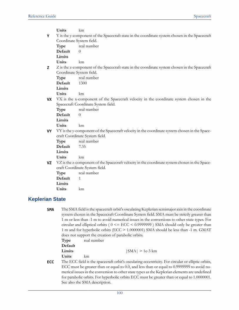
Reference Guide Spacecraft
100
Units kmY Y is the y-component of the Spacecraft state in the coordinate system chosen in the Spacecraft
Coordinate System field.Type real numberDefault 0LimitsUnits km
Z Z is the z-component of the Spacecraft state in the coordinate system chosen in the SpacecraftCoordinate System field.Type real numberDefault 1300LimitsUnits km
VX VX is the x-component of the Spacecraft velocity in the coordinate system chosen in theSpacecraft Coordinate System field.Type real numberDefault 0LimitsUnits km
VY VY is the y-component of the Spacecraft velocity in the coordinate system chosen in the Space-craft Coordinate System field.Type real numberDefault 7.35LimitsUnits km
VZ VZ is the z-component of the Spacecraft velocity in the coordinate system chosen in the Space-craft Coordinate System field.Type real numberDefault 1LimitsUnits km
Keplerian State
SMA The SMA field is the spacecraft orbit's osculating Keplerian semimajor axis in the coordinatesystem chosen in the Spacecraft Coordinate System field. SMA must be strictly greater than1 m or less than -1 m to avoid numerical issues in the conversions to other state types. Forcircular and elliptical orbits ( 0 <= ECC < 0.9999999 ) SMA should only be greater than1 m and for hyperbolic orbits (ECC > 1.0000001) SMA should be less than -1 m. GMATdoes not support the creation of parabolic orbits.Type real numberDefaultLimits |SMA| > 1e-3 kmUnits km
ECC The ECC field is the spacecraft orbit's osculating eccentricity. For circular or elliptic orbits,ECC must be greater than or equal to 0.0, and less than or equal to 0.9999999 to avoid nu-merical issues in the conversion to other state types as the Keplerian elements are undefinedfor parabolic orbits. For hyperbolic orbits ECC must be greater than or equal to 1.0000001.See also the SMA description.
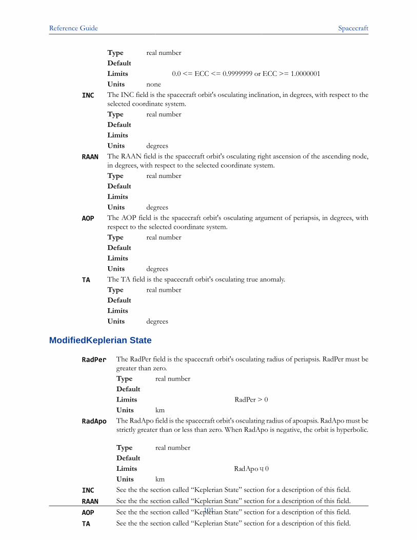
Reference Guide Spacecraft
101
Type real numberDefaultLimits 0.0 <= ECC <= 0.9999999 or ECC >= 1.0000001Units none
INC The INC field is the spacecraft orbit's osculating inclination, in degrees, with respect to theselected coordinate system.Type real numberDefaultLimitsUnits degrees
RAAN The RAAN field is the spacecraft orbit's osculating right ascension of the ascending node,in degrees, with respect to the selected coordinate system.Type real numberDefaultLimitsUnits degrees
AOP The AOP field is the spacecraft orbit's osculating argument of periapsis, in degrees, withrespect to the selected coordinate system.Type real numberDefaultLimitsUnits degrees
TA The TA field is the spacecraft orbit's osculating true anomaly.Type real numberDefaultLimitsUnits degrees
ModifiedKeplerian State
RadPer The RadPer field is the spacecraft orbit's osculating radius of periapsis. RadPer must begreater than zero.Type real numberDefaultLimits RadPer > 0Units km
RadApo The RadApo field is the spacecraft orbit's osculating radius of apoapsis. RadApo must bestrictly greater than or less than zero. When RadApo is negative, the orbit is hyperbolic.
Type real numberDefaultLimitsUnits km
INC See the the section called “Keplerian State” section for a description of this field.
RAAN See the the section called “Keplerian State” section for a description of this field.
AOP See the the section called “Keplerian State” section for a description of this field.
TA See the the section called “Keplerian State” section for a description of this field.
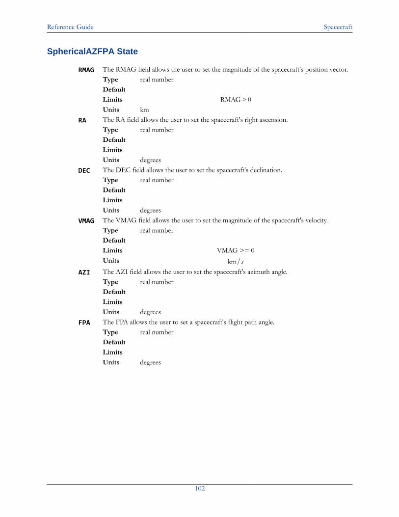
Reference Guide Spacecraft
102
SphericalAZFPA State
RMAG The RMAG field allows the user to set the magnitude of the spacecraft's position vector.Type real numberDefaultLimitsUnits km
RA The RA field allows the user to set the spacecraft's right ascension.Type real numberDefaultLimitsUnits degrees
DEC The DEC field allows the user to set the spacecraft's declination.Type real numberDefaultLimitsUnits degrees
VMAG The VMAG field allows the user to set the magnitude of the spacecraft's velocity.Type real numberDefaultLimits VMAG >= 0Units
AZI The AZI field allows the user to set the spacecraft's azimuth angle.Type real numberDefaultLimitsUnits degrees
FPA The FPA allows the user to set a spacecraft's flight path angle.Type real numberDefaultLimitsUnits degrees
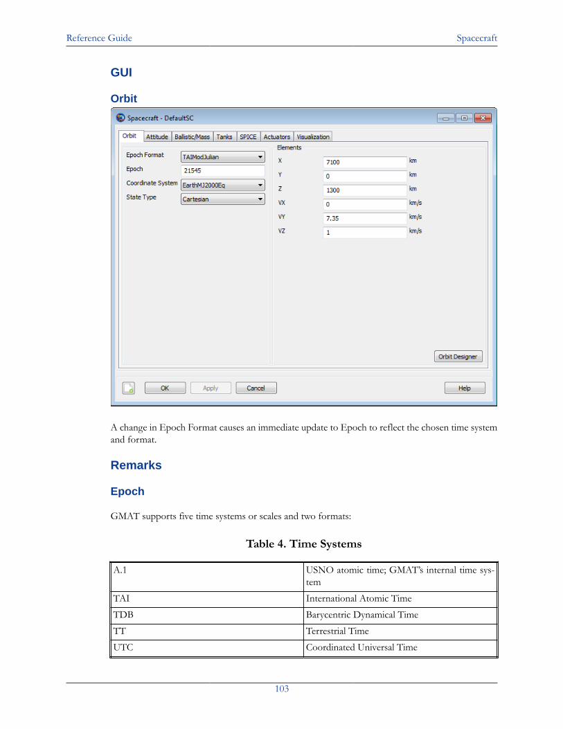
Reference Guide Spacecraft
103
GUI
Orbit
A change in Epoch Format causes an immediate update to Epoch to reflect the chosen time systemand format.
Remarks
Epoch
GMAT supports five time systems or scales and two formats:
Table 4. Time Systems
A.1 USNO atomic time; GMAT’s internal time sys-tem
TAI International Atomic Time
TDB Barycentric Dynamical Time
TT Terrestrial Time
UTC Coordinated Universal Time
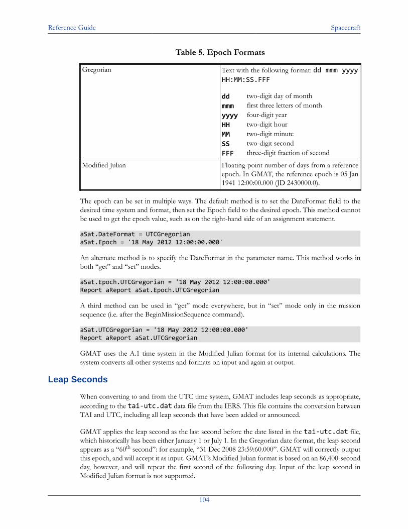
Reference Guide Spacecraft
104
Table 5. Epoch Formats
Gregorian Text with the following format: dd mmm yyyyHH:MM:SS.FFF
dd two-digit day of monthmmm first three letters of monthyyyy four-digit yearHH two-digit hourMM two-digit minuteSS two-digit secondFFF three-digit fraction of second
Modified Julian Floating-point number of days from a referenceepoch. In GMAT, the reference epoch is 05 Jan1941 12:00:00.000 (JD 2430000.0).
The epoch can be set in multiple ways. The default method is to set the DateFormat field to thedesired time system and format, then set the Epoch field to the desired epoch. This method cannotbe used to get the epoch value, such as on the right-hand side of an assignment statement.
aSat.DateFormat = UTCGregorianaSat.Epoch = '18 May 2012 12:00:00.000'
An alternate method is to specify the DateFormat in the parameter name. This method works inboth “get” and “set” modes.
aSat.Epoch.UTCGregorian = '18 May 2012 12:00:00.000'Report aReport aSat.Epoch.UTCGregorian
A third method can be used in “get” mode everywhere, but in “set” mode only in the missionsequence (i.e. after the BeginMissionSequence command).
aSat.UTCGregorian = '18 May 2012 12:00:00.000'Report aReport aSat.UTCGregorian
GMAT uses the A.1 time system in the Modified Julian format for its internal calculations. Thesystem converts all other systems and formats on input and again at output.
Leap Seconds
When converting to and from the UTC time system, GMAT includes leap seconds as appropriate,according to the tai-utc.dat data file from the IERS. This file contains the conversion betweenTAI and UTC, including all leap seconds that have been added or announced.
GMAT applies the leap second as the last second before the date listed in the tai-utc.dat file,which historically has been either January 1 or July 1. In the Gregorian date format, the leap secondappears as a “60th second”: for example, “31 Dec 2008 23:59:60.000”. GMAT will correctly outputthis epoch, and will accept it as input. GMAT’s Modified Julian format is based on an 86,400-secondday, however, and will repeat the first second of the following day. Input of the leap second inModified Julian format is not supported.
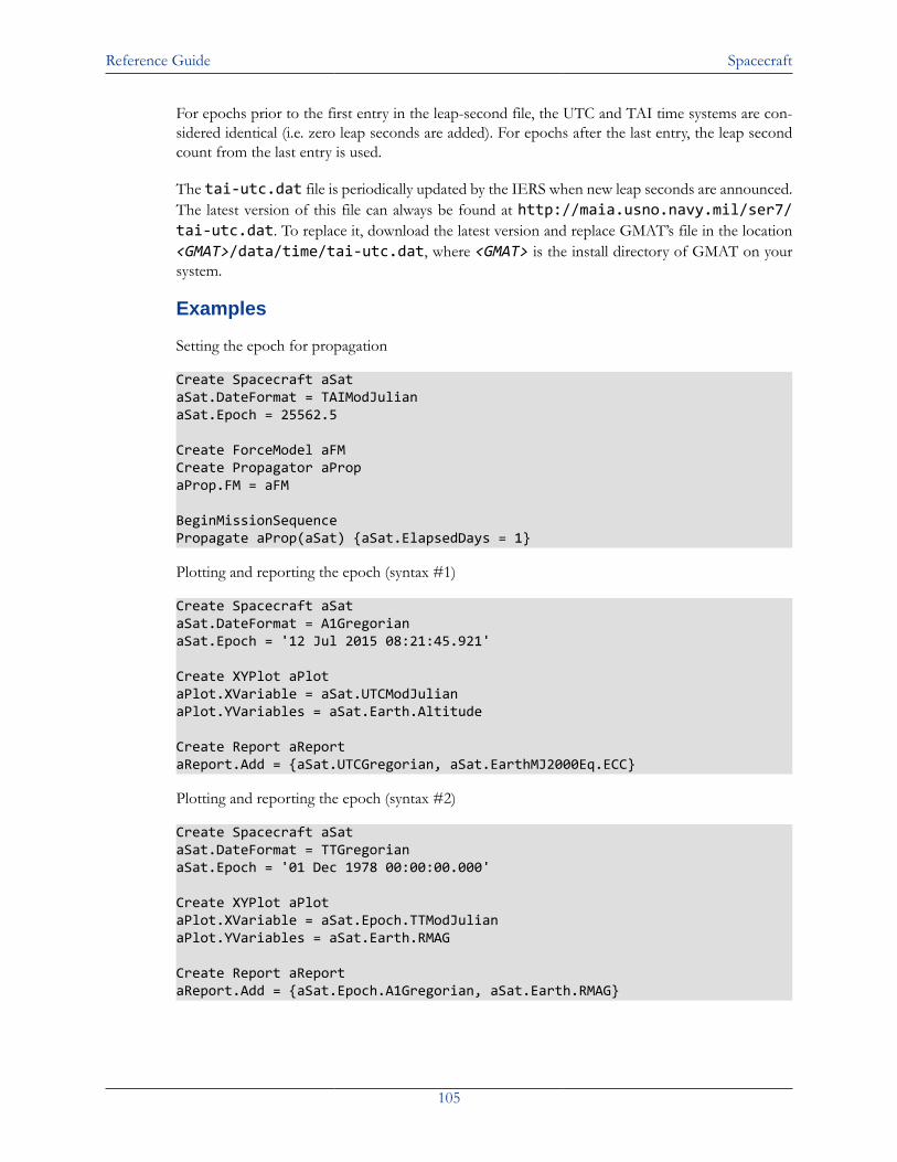
Reference Guide Spacecraft
105
For epochs prior to the first entry in the leap-second file, the UTC and TAI time systems are con-sidered identical (i.e. zero leap seconds are added). For epochs after the last entry, the leap secondcount from the last entry is used.
The tai-utc.dat file is periodically updated by the IERS when new leap seconds are announced.The latest version of this file can always be found at http://maia.usno.navy.mil/ser7/tai-utc.dat. To replace it, download the latest version and replace GMAT’s file in the location<GMAT>/data/time/tai-utc.dat, where <GMAT> is the install directory of GMAT on yoursystem.
Examples
Setting the epoch for propagation
Create Spacecraft aSataSat.DateFormat = TAIModJulianaSat.Epoch = 25562.5
Create ForceModel aFMCreate Propagator aPropaProp.FM = aFM
BeginMissionSequencePropagate aProp(aSat) {aSat.ElapsedDays = 1}
Plotting and reporting the epoch (syntax #1)
Create Spacecraft aSataSat.DateFormat = A1GregorianaSat.Epoch = '12 Jul 2015 08:21:45.921'
Create XYPlot aPlotaPlot.XVariable = aSat.UTCModJulianaPlot.YVariables = aSat.Earth.Altitude
Create Report aReportaReport.Add = {aSat.UTCGregorian, aSat.EarthMJ2000Eq.ECC}
Plotting and reporting the epoch (syntax #2)
Create Spacecraft aSataSat.DateFormat = TTGregorianaSat.Epoch = '01 Dec 1978 00:00:00.000'
Create XYPlot aPlotaPlot.XVariable = aSat.Epoch.TTModJulianaPlot.YVariables = aSat.Earth.RMAG
Create Report aReportaReport.Add = {aSat.Epoch.A1Gregorian, aSat.Earth.RMAG}
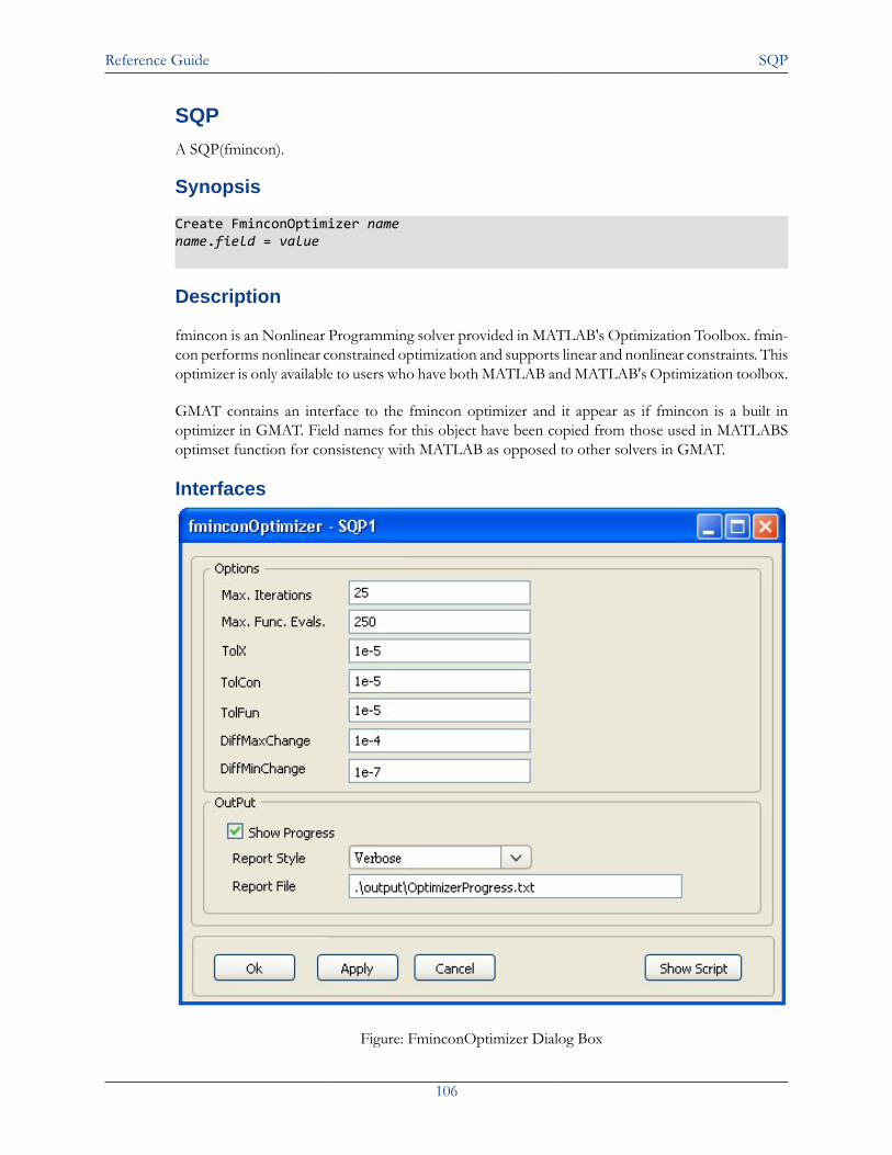
Reference Guide SQP
106
SQP
A SQP(fmincon).
Synopsis
Create FminconOptimizer namename.field = value
Description
fmincon is an Nonlinear Programming solver provided in MATLAB's Optimization Toolbox. fmin-con performs nonlinear constrained optimization and supports linear and nonlinear constraints. Thisoptimizer is only available to users who have both MATLAB and MATLAB's Optimization toolbox.
GMAT contains an interface to the fmincon optimizer and it appear as if fmincon is a built inoptimizer in GMAT. Field names for this object have been copied from those used in MATLABSoptimset function for consistency with MATLAB as opposed to other solvers in GMAT.
Interfaces
Figure: FminconOptimizer Dialog Box
Reference Guide SQP
107
Fields
DiffMax Change The DiffMaxChange parameter is the upper limit on the perturbation usedin MATLAB's finite differencing algorithm. For fmincon, you don't specifya single perturbation value, but rather give MATLAB a range, and it uses anadaptive algorithm that attempts to find the optimal perturbation.Default 0.1Limits Real Number > 0Units None
DiffMin Change The DiffMinChange parameter is the lower limit on the perturbation usedin MATLAB's finite differencing algorithm. For fmincon, you don't specifya single perturbation value, but rather give MATLAB a range, and it uses anadaptive algorithm that attempts to find the optimal perturbatin.Default 1e-8Limits Real Number > 0Units None
MaxFunEvals The MaxFunEvals parameter allows the user to set the maximum number ofcost function evaluations in an attempt to find an optimal solution. This isequivalent to setting the maximum number of passes through an optimiza-tion loop in a GMAT script. If a solution is not found before the maximumfunction evaluations, fmincon outputs an ExitFlag of zero, and GMAT con-tinues.Default 1000Limits Integer > 0Units None
MaxIter The MaxIter parameter allows the user to set the maximum allowable num-ber of optimizer iterations. Depending upon the nature of the problem, andwhether gradients are provided, it may take many function evaluations foreach optimizer iteration. The MaxIter parameter allows the user to controlthe maximum function evaluations, and maximum iterations independently.Default 400Limits Integer > 0Units None
TolX The TolX parameter is the termination toler-ance on the vector of indepen-dent variables, and is used only if the user sets a value.Default 1e-4Limits Real Number > 0Units None
TolFun The TolFun parameter is the convergence tolerance on the cost functionvalue.Default 1e-4Limits Real Number > 0Units None
TolCon The TolCon parameter is the convergence tolerance on the constraint func-tions.Default 1e-4Limits Real Number > 0Units None
Reference Guide SQP
108
ShowProgress The ShowProgress field determines whether data pertaining to iterations ofthe solver is displayed in the message window. When ShowProgress is true,the amount of information contained in the message window is controlledby the ReportSytle field.Default trueLimits true, falseUnits None
ReportStyle The ReportStyel field determines the amount and type of data written tothe message window for each iteration of the solver (When ShowProgressis true). ADD DESCRIPTIONS OF CONCISE,VERBOSE, ADN NOR-MAL. I CAN'T RUN THE OPTIMIZER RIGHT NOW SO I CAN'TTELL WHAT EACH SETTING DOES.Default NormalLimits Normal, Concise, Verbose, DebugUnits None
ReportFile The ReportFile field contains the path and file name of the report file.Default NormalLimits .\output\OptimizerData.txtUnits None
Using an fminconOptimizer
• Optimize Command• Minimize• Nonlinear Constraint
Examples
Create FminconOptimizer SQP1;GMAT SQP1.MaxIter = 25;GMAT SQP1.MaxFunEvals = 250;GMAT SQP1.TolX = 1e-5;GMAT SQP1.TolFun = 1e-5;GMAT SQP1.TolCon = 1e-5;GMAT SQP1.DiffMaxChange = 1e-4;GMAT SQP1.DiffMinChange = 1e-7;GMAT SQP1.ShowProgress = true;GMAT SQP1.ReportStyle = 'Verbose';GMAT SQP1.ReportFile = '\output\OptimizerProgress.txt';
Reference Guide String
109
StringA string.
Synopsis
Create String namename.field = value
Description
This page will show you how to create and use String objects. Stings are useful for storing charactersas a set. One possible use of them is to report back a specific message at a set point in the missionsequence.
Interactions
ReportFile You may add a string to the Parameter List in the Report Object dialog boxvia the ParameterSelectDialog box.
Report Command Alternatively, you may add a string to the Parameter List in the Report Com-mand dialog box
Using the Script
Script Syntax
GMAT String Name = String;
Script Examples
% The following is an example String declarationGMAT Example = hello world;
Reference Guide Thruster
110
Thruster
A thruster.
Synopsis
Create Thruster namename.field = value
Description
The Thruster uses the fuel tank and directs the thrust of the rocket engine while in space. It is usedfor finite burns.
Fields
CoordinateSystem The CoordinateSystem field for a thrusterdetermines what coordi-nate system the orientation parametersX_Direction, Y_Direction, andZ_Direction arereferenced to. This is a temporary fix in GMAT.Eventually, theuser will specify the attitude of aspacecraft, and thenX_Direction, Y_Direction, and Z_Direction will be referenced to thespacecraft body frame.Default EarthMJ2000EqLimits EarthMJ2000Eq, EarthMJ2000Ec, EarthMJ2000Eq, or
anyuser defined systemAxis The Axis field allows the user to define a localcoordinate system for a
thruster. Note that there is a couplingbetween the Axis parameter andthe CoordinateSystemparameter for a thruster. Only one of the twocanbe specified.Default VNBLimits InertialVNBUnits None
Origin The Origin fieldallows the user to define a local origin for a thruster.Note thatthere is a coupling between the Origin parameter and theCo-ordinateSystem parameter for a thruster. Only one of the twocan bespecified.Default EarthLimits Sun, Mercury, Venus, Earth, Luna, Mars,Jupiter, Saturn,
Uranus, Neptune, PlutoUnits None
X_Direction X_Direction, divided by the RSS of the three directioncomponents,forms the x direction of the spacecraft thrust vector direction.Default 1Limits Real Number
Y_Direction Y_Direction, divided by the RSS of the three directioncomponents,forms the y direction of the spacecraft thrust vector direction.Default 0Limits Real Number
Reference Guide Thruster
111
Z_Direction Z_Direction, divided by the RSS of the three directioncomponents,forms the z direction of the spacecraft thrust vector direction.Default 0Limits Real Number
ThrustScaleFactor ThrustScaleFactor is a scale factor that is multiplied by the thrust vectorfor a given thruster, before the thrust vector is added into the totalaccleration.Default 1Limits Real Number > 0Units None
Tank The Tank field specifies which tank the thruster draws propellant from.
The constants Ci below are used in the following equation to calculatethrust FT as a function of pressure P and temperature TDefault NoneLimits Tank NameUnits FT(P,T) = {C1+C2P+C3P2+C4PC5+C6PC7+C8PC9
+C10C11C12P}(T/Tref)1+C13+C14P
C1 Thrust coefficient.Default 500Limits Real NumberUnits N
C2 Thrust coefficient.Default 0Limits Real NumberUnits N/kPa
C3 Thrust coefficient.Default 0Limits Real NumberUnits N/kPa
C4 Thrust coefficient.Default 0Limits Real NumberUnits N/kPaC5
C5 Thrust coefficient.Default 0Limits Real NumberUnits None
C6 Thrust coefficient.Default 0Limits Real NumberUnits N/kPaC7
C7 Thrust coefficient.Default 0Limits Real NumberUnits None
C8 Thrust coefficient.Default 0Limits Real Number

Reference Guide Thruster
112
Units N/kPaC9
C9 Thrust coefficient.Default 0Limits Real NumberUnits None
C10 Thrust coefficient.Default 0Limits Real NumberUnits N
C11 Thrust coefficient.Default 1Limits Real NumberUnits None
C12 Thrust coefficient.Default 0Limits Real NumberUnits 1/kPa
C13 Thrust coefficient.Default 0Limits Real NumberUnits None
C14 Thrust coefficient.Default 0Limits Real NumberUnits 1/kPaThe constants Ki below are usedin the following equation tocalcu-late Isp as a function of pressureP and temperatureT
Isp(P,T)   =  {K1+K2P+K3P2+K4PK5+K6PK7+K8PK9+K10K11
K12P} (T/Tref)1+K13+K14P
K1 Isp coefficient.Default 2150Limits Real NumberUnits m/sec
K2 Isp coefficient.Default 0Limits Real NumberUnits m/(sec?kPa)
K3 Isp coefficient.Default 0Limits Real NumberUnits m/(sec?kPa2)
K4 Isp coefficient.Default 0Limits Real NumberUnits m/(sec?kPaK5)
K5 Isp coefficient.Default 0Limits Real Number
Reference Guide Thruster
113
Units NoneK6 Isp coefficient.
Default 0Limits Real NumberUnits m/(sec?kPaK7)
K7 Isp coefficient.Default 0Limits Real NumberUnits None
K8 Isp coefficient.Default 0Limits Real NumberUnits m/(sec?kPaK9
K9 Isp coefficient.Default 0Limits Real NumberUnits None
K10 Isp coefficient.Default 0Limits Real NumberUnits m/sec
K11 Isp coefficient.Default 1Limits Real NumberUnits None
K12 Isp coefficient.Default 0Limits Real NumberUnits 1/kPa
K13 Isp coefficient.Default 0Limits Real NumberUnits None
K14 Isp coefficient.Default 0Limits Real NumberUnits 1/kPa
Interactions
BeginFiniteBurn/EndFiniteBurn These commands use the tank and the thruster to start afinite burn, where the delta V is not instantaneous.
Fuel Tank This object contains the fuel used to power the thruster andsubsequently the finite burn.
FiniteBurn This takes the parameters of the tank and the thruster andapply it to a coordinate system, with a scaling method avail-able if wanted.
Spacecraft This is the object that the burn is applied to.
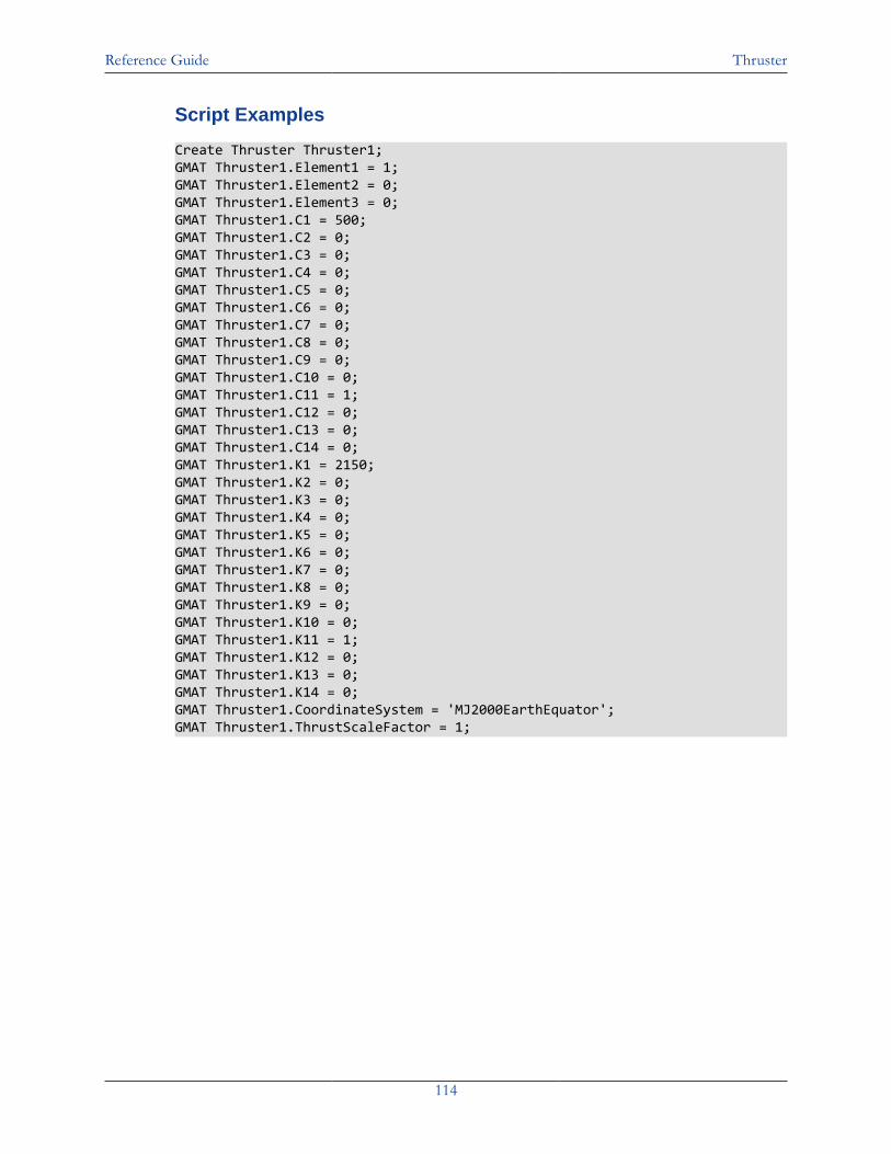
Reference Guide Thruster
114
Script Examples
Create Thruster Thruster1;GMAT Thruster1.Element1 = 1;GMAT Thruster1.Element2 = 0;GMAT Thruster1.Element3 = 0;GMAT Thruster1.C1 = 500;GMAT Thruster1.C2 = 0;GMAT Thruster1.C3 = 0;GMAT Thruster1.C4 = 0;GMAT Thruster1.C5 = 0;GMAT Thruster1.C6 = 0;GMAT Thruster1.C7 = 0;GMAT Thruster1.C8 = 0;GMAT Thruster1.C9 = 0;GMAT Thruster1.C10 = 0;GMAT Thruster1.C11 = 1;GMAT Thruster1.C12 = 0;GMAT Thruster1.C13 = 0;GMAT Thruster1.C14 = 0;GMAT Thruster1.K1 = 2150;GMAT Thruster1.K2 = 0;GMAT Thruster1.K3 = 0;GMAT Thruster1.K4 = 0;GMAT Thruster1.K5 = 0;GMAT Thruster1.K6 = 0;GMAT Thruster1.K7 = 0;GMAT Thruster1.K8 = 0;GMAT Thruster1.K9 = 0;GMAT Thruster1.K10 = 0;GMAT Thruster1.K11 = 1;GMAT Thruster1.K12 = 0;GMAT Thruster1.K13 = 0;GMAT Thruster1.K14 = 0;GMAT Thruster1.CoordinateSystem = 'MJ2000EarthEquator';GMAT Thruster1.ThrustScaleFactor = 1;
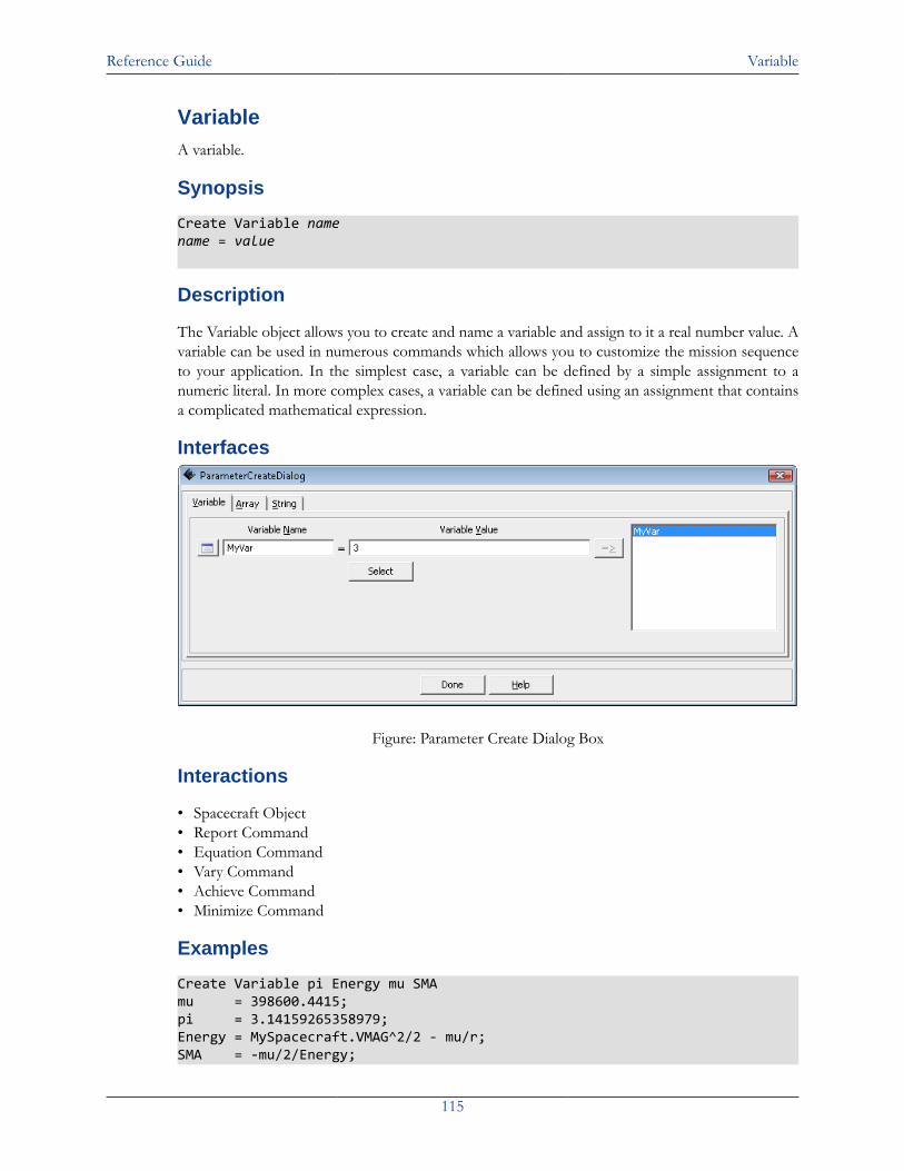
Reference Guide Variable
115
VariableA variable.
Synopsis
Create Variable namename = value
Description
The Variable object allows you to create and name a variable and assign to it a real number value. Avariable can be used in numerous commands which allows you to customize the mission sequenceto your application. In the simplest case, a variable can be defined by a simple assignment to anumeric literal. In more complex cases, a variable can be defined using an assignment that containsa complicated mathematical expression.
Interfaces
Figure: Parameter Create Dialog Box
Interactions
• Spacecraft Object• Report Command• Equation Command• Vary Command• Achieve Command• Minimize Command
Examples
Create Variable pi Energy mu SMAmu = 398600.4415;pi = 3.14159265358979;Energy = MySpacecraft.VMAG^2/2 - mu/r; SMA = -mu/2/Energy;
Reference Guide VF13adOptimizer
116
VF13adOptimizerUnder Construction.
Synopsis
Under Construction.
Description
Under Construction.
Fields
Field Name Description....Type Fill This In.Default Fill This In.Limits Fill This In.Units Fill This In.
Examples
Example 10. Example Script
%
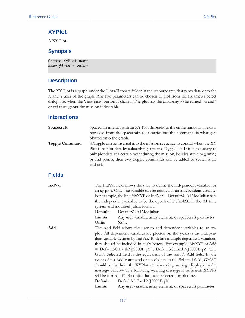
Reference Guide XYPlot
117
XYPlotA XY Plot.
Synopsis
Create XYPlot namename.field = value
Description
The XY Plot is a graph under the Plots/Reports folder in the resource tree that plots data onto theX and Y axes of the graph. Any two parameters can be chosen to plot from the Parameter Selectdialog box when the View radio button is clicked. The plot has the capability to be turned on and/or off throughout the mission if desirable.
Interactions
Spacecraft Spacecraft interact with an XY Plot throughout the entire mission. The dataretrieved from the spacecraft, as it carries out the command, is what getsplotted onto the graph.
Toggle Command A Toggle can be inserted into the mission sequence to control when the XYPlot is to plot data by subscribing it to the Toggle list. If it is necessary toonly plot data at a certain point during the mission, besides at the beginningor end points, then two Toggle commands can be added to switch it onand off.
Fields
IndVar The IndVar field allows the user to define the independent variable foran xy-plot. Only one variable can be defined as an independent variable.For example, the line MyXYPlot.IndVar = DefaultSC.A1ModJulian setsthe independent variable to be the epoch of DefaultSC in the A1 timesystem and modified Julian format.Default DefaultSC.A1ModJulianLimits Any user variable, array element, or spacecraft parameterUnits None
Add The Add field allows the user to add dependent variables to an xy-plot. All dependent variables are plotted on the y-axisvs the indepen-dent variable defined by IndVar. To define multiple dependent variables,they should be included in curly braces. For example, MyXYPlot.Add= DefaultSC.EarthMJ2000Eq.Y , DefaultSC.EarthMJ2000Eq.Z. TheGUI's Selected field is the equivalent of the script's Add field. In theevent of no Add command or no objects in the Selected field, GMATshould run without the XYPlot and a warning message displayed in themessage window. The following warning message is sufficient: XYPlotwill be turned off. No object has been selected for plotting.Default DefaultSC.EarthMJ2000Eq.XLimits Any user variable, array element, or spacecraft parameter
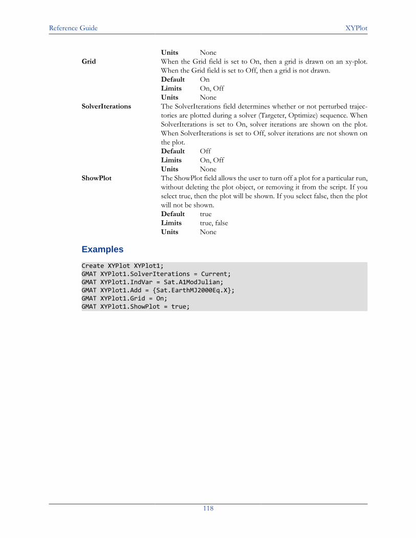
Reference Guide XYPlot
118
Units NoneGrid When the Grid field is set to On, then a grid is drawn on an xy-plot.
When the Grid field is set to Off, then a grid is not drawn.Default OnLimits On, OffUnits None
SolverIterations The SolverIterations field determines whether or not perturbed trajec-tories are plotted during a solver (Targeter, Optimize) sequence. WhenSolverIterations is set to On, solver iterations are shown on the plot.When SolverIterations is set to Off, solver iterations are not shown onthe plot.Default OffLimits On, OffUnits None
ShowPlot The ShowPlot field allows the user to turn off a plot for a particular run,without deleting the plot object, or removing it from the script. If youselect true, then the plot will be shown. If you select false, then the plotwill not be shown.Default trueLimits true, falseUnits None
Examples
Create XYPlot XYPlot1;GMAT XYPlot1.SolverIterations = Current;GMAT XYPlot1.IndVar = Sat.A1ModJulian;GMAT XYPlot1.Add = {Sat.EarthMJ2000Eq.X};GMAT XYPlot1.Grid = On;GMAT XYPlot1.ShowPlot = true;

Reference Guide Commands
119
Commands
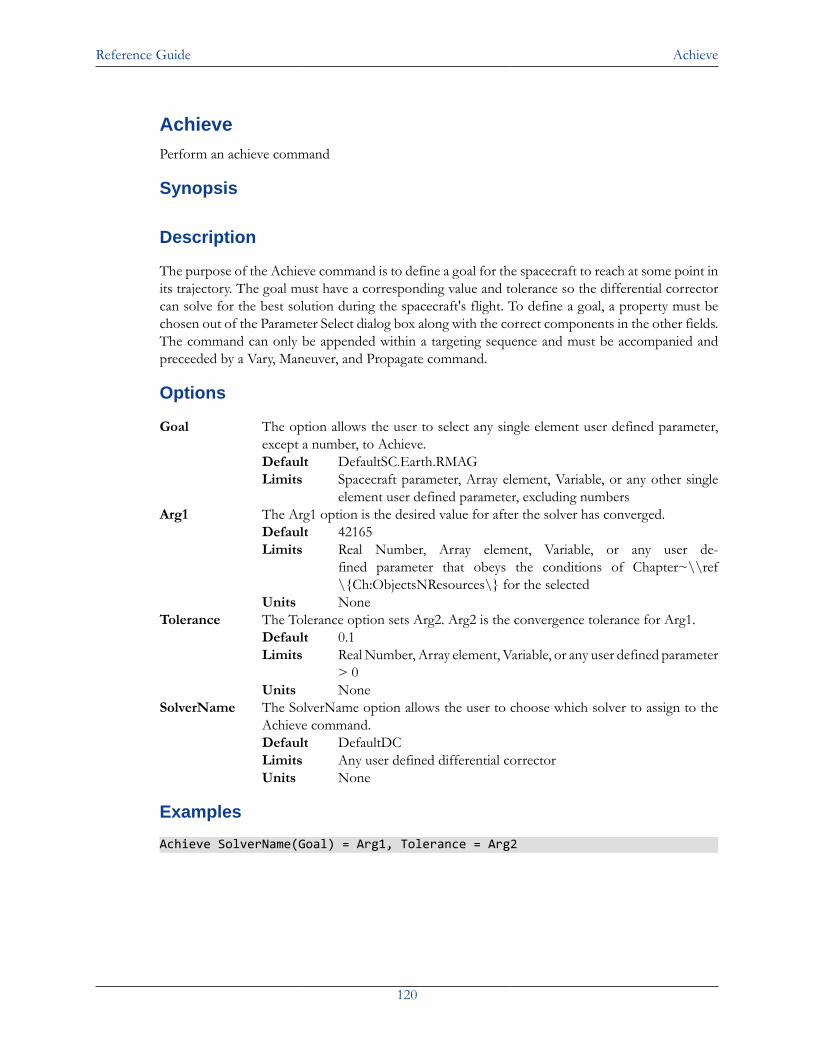
Reference Guide Achieve
120
AchievePerform an achieve command
Synopsis
Description
The purpose of the Achieve command is to define a goal for the spacecraft to reach at some point inits trajectory. The goal must have a corresponding value and tolerance so the differential correctorcan solve for the best solution during the spacecraft's flight. To define a goal, a property must bechosen out of the Parameter Select dialog box along with the correct components in the other fields.The command can only be appended within a targeting sequence and must be accompanied andpreceeded by a Vary, Maneuver, and Propagate command.
Options
Goal The option allows the user to select any single element user defined parameter,except a number, to Achieve.Default DefaultSC.Earth.RMAGLimits Spacecraft parameter, Array element, Variable, or any other single
element user defined parameter, excluding numbersArg1 The Arg1 option is the desired value for after the solver has converged.
Default 42165Limits Real Number, Array element, Variable, or any user de-
fined parameter that obeys the conditions of Chapter~\\ref\{Ch:ObjectsNResources\} for the selected
Units NoneTolerance The Tolerance option sets Arg2. Arg2 is the convergence tolerance for Arg1.
Default 0.1Limits Real Number, Array element, Variable, or any user defined parameter
> 0Units None
SolverName The SolverName option allows the user to choose which solver to assign to theAchieve command.Default DefaultDCLimits Any user defined differential correctorUnits None
Examples
Achieve SolverName(Goal) = Arg1, Tolerance = Arg2
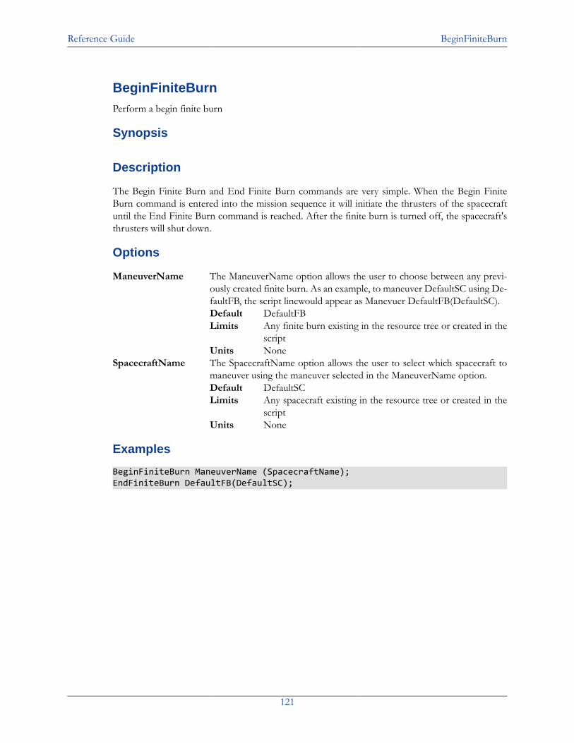
Reference Guide BeginFiniteBurn
121
BeginFiniteBurnPerform a begin finite burn
Synopsis
Description
The Begin Finite Burn and End Finite Burn commands are very simple. When the Begin FiniteBurn command is entered into the mission sequence it will initiate the thrusters of the spacecraftuntil the End Finite Burn command is reached. After the finite burn is turned off, the spacecraft'sthrusters will shut down.
Options
ManeuverName The ManeuverName option allows the user to choose between any previ-ously created finite burn. As an example, to maneuver DefaultSC using De-faultFB, the script linewould appear as Manevuer DefaultFB(DefaultSC).Default DefaultFBLimits Any finite burn existing in the resource tree or created in the
scriptUnits None
SpacecraftName The SpacecraftName option allows the user to select which spacecraft tomaneuver using the maneuver selected in the ManeuverName option.Default DefaultSCLimits Any spacecraft existing in the resource tree or created in the
scriptUnits None
Examples
BeginFiniteBurn ManeuverName (SpacecraftName); EndFiniteBurn DefaultFB(DefaultSC);
Reference Guide BeginMissionSequence
122
BeginMissionSequenceUnder construction.
Synopsis
Under construction.
Under construction.
Under construction.
Examples
Script Syntax
Under construction.
Script Examples
Under construction.
Reference Guide CallGmatFunction
123
CallGmatFunctionCall a GMAT function
Synopsis
<incomplete>
Definition
GMAT functions are very useful and work nearly the same as they do in most programming lan-guages. They may be invoked using the CallGmatFunction command covered here.
Options
OutputList The OutputList option allows the user to set the output of Function to a userdefined parameter.Default NoneLimits Variables, Arrays, S/C, Paramters, any other user-defined parame-
ters, or blank. Multiple outputs must be expressed in a comma de-limited list format
Units NoneInputList The InputList option allows the user to set the input of Function to a user defined
parameter.Default NoneLimits Variables, Arrays, S/C, Paramters, any other user-defined parame-
ters, or blank. Multiple inputs must be expressed in a comma delim-ited list format.
Units NoneFunction The Function option allows the user to set the function that will be called in a
specific location of the mission sequence. The function has to be defined beforeit can be used in the CallFunction Command.Default NoneLimits GMAT of Matlab FunctionUnits None
Examples
Script Syntax
%Function call with Inputs and OutputsGMAT [OutputList] = Function(InputList)
%Function call with Outputs onlyGMAT [OutputList] = Function
%Function call with Inputs onlyGMAT Function(InputList)
Function call with no Inputs or Outputs
Reference Guide CallGmatFunction
124
GMAT Function
Script Examples
% Matlab function call without inputs or outputs
% Syntax 1GMAT clearAll
% Syntax 2GMAT [ ] = clearAll( )
Reference Guide CallMatlabFunction
125
CallMatlabFunctionCall a MATLAB function
Script Syntax
<incomplete>
Description
This reference page is incomplete at this time.
Reference Guide ClearPlot
126
ClearPlotClear a graphical plot window
Script Syntax
<incomplete>
Description
This reference page is incomplete at this time.
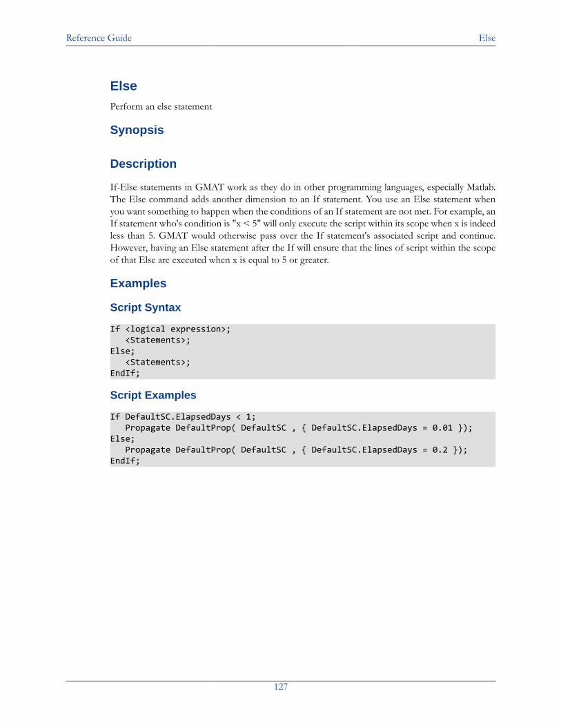
Reference Guide Else
127
ElsePerform an else statement
Synopsis
Description
If-Else statements in GMAT work as they do in other programming languages, especially Matlab.The Else command adds another dimension to an If statement. You use an Else statement whenyou want something to happen when the conditions of an If statement are not met. For example, anIf statement who's condition is "x < 5" will only execute the script within its scope when x is indeedless than 5. GMAT would otherwise pass over the If statement's associated script and continue.However, having an Else statement after the If will ensure that the lines of script within the scopeof that Else are executed when x is equal to 5 or greater.
Examples
Script Syntax
If <logical expression>; <Statements>;Else; <Statements>;EndIf;
Script Examples
If DefaultSC.ElapsedDays < 1; Propagate DefaultProp( DefaultSC , { DefaultSC.ElapsedDays = 0.01 });Else; Propagate DefaultProp( DefaultSC , { DefaultSC.ElapsedDays = 0.2 });EndIf;
Reference Guide EndFiniteBurn
128
EndFiniteBurnUnder construction.
Synopsis
Under construction.
Under construction.
Under construction.
Examples
Script Syntax
Under construction.
Script Examples
Under construction.
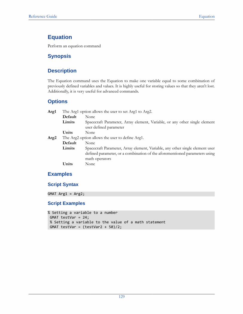
Reference Guide Equation
129
EquationPerform an equation command
Synopsis
Description
The Equation command uses the Equation to make one variable equal to some combination ofpreviously defined variables and values. It is highly useful for storing values so that they aren't lost.Additionally, it is very useful for advanced commands.
Options
Arg1 The Arg1 option allows the user to set Arg1 to Arg2.Default NoneLimits Spacecraft Parameter, Array element, Variable, or any other single element
user defined parameterUnits None
Arg2 The Arg2 option allows the user to define Arg1.Default NoneLimits Spacecraft Parameter, Array element, Variable, any other single element user
defined parameter, or a combination of the aforementioned parameters usingmath operators
Units None
Examples
Script Syntax
GMAT Arg1 = Arg2;
Script Examples
% Setting a variable to a number GMAT testVar = 24; % Setting a variable to the value of a math statement GMAT testVar = (testVar2 + 50)/2;
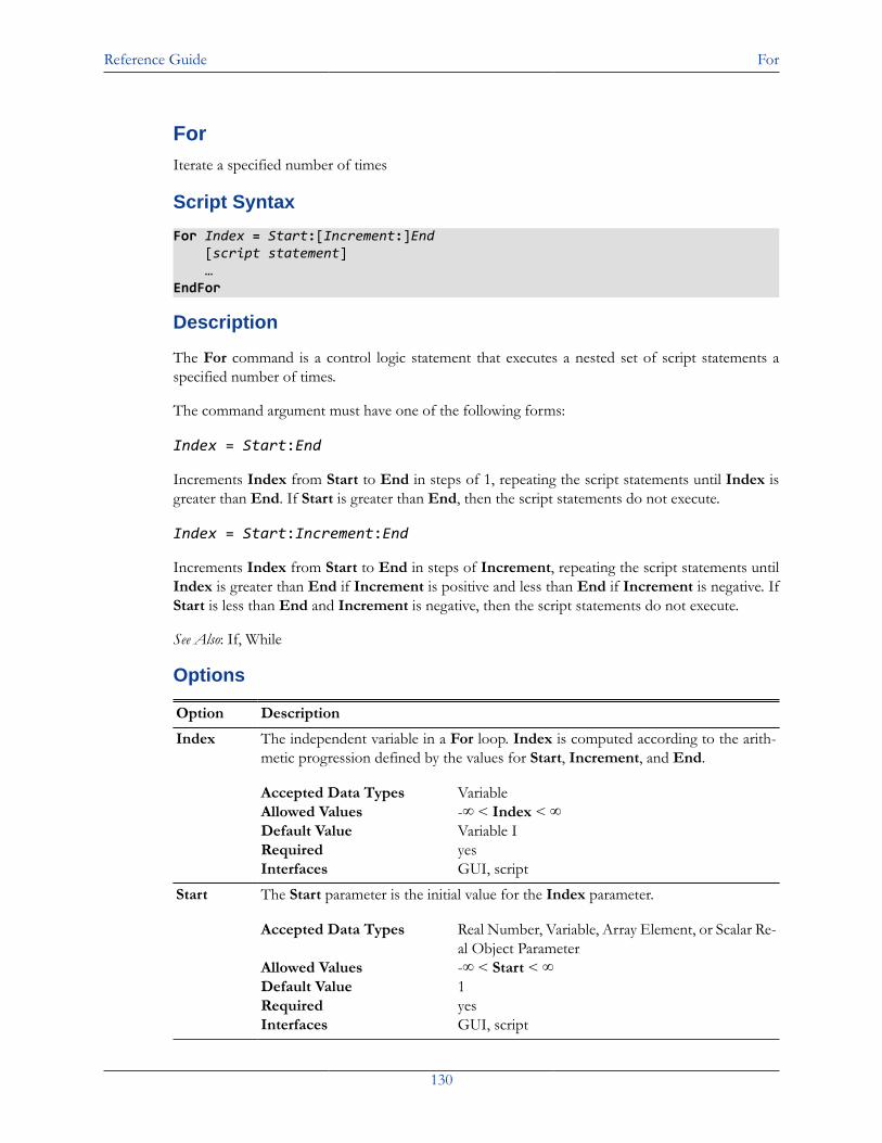
Reference Guide For
130
ForIterate a specified number of times
Script Syntax
For Index = Start:[Increment:]End [script statement] …EndFor
Description
The For command is a control logic statement that executes a nested set of script statements aspecified number of times.
The command argument must have one of the following forms:
Index = Start:End
Increments Index from Start to End in steps of 1, repeating the script statements until Index isgreater than End. If Start is greater than End, then the script statements do not execute.
Index = Start:Increment:End
Increments Index from Start to End in steps of Increment, repeating the script statements untilIndex is greater than End if Increment is positive and less than End if Increment is negative. IfStart is less than End and Increment is negative, then the script statements do not execute.
See Also: If, While
Options
Option Description
Index The independent variable in a For loop. Index is computed according to the arith-metic progression defined by the values for Start, Increment, and End.
Accepted Data Types VariableAllowed Values -∞ < Index < ∞Default Value Variable IRequired yesInterfaces GUI, script
Start The Start parameter is the initial value for the Index parameter.
Accepted Data Types Real Number, Variable, Array Element, or Scalar Re-al Object Parameter
Allowed Values -∞ < Start < ∞Default Value 1Required yesInterfaces GUI, script
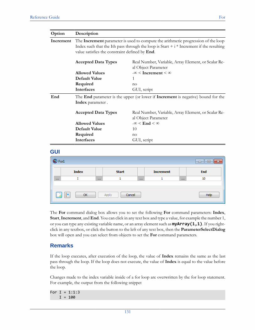
Reference Guide For
131
Option Description
Increment The Increment parameter is used to compute the arithmetic progression of the loopIndex such that the Ith pass through the loop is Start + i * Increment if the resultingvalue satisfies the constraint defined by End.
Accepted Data Types Real Number, Variable, Array Element, or Scalar Re-al Object Parameter
Allowed Values -∞ < Increment < ∞Default Value 1Required noInterfaces GUI, script
End The End parameter is the upper (or lower if Increment is negative) bound for theIndex parameter .
Accepted Data Types Real Number, Variable, Array Element, or Scalar Re-al Object Parameter
Allowed Values -∞ < End < ∞Default Value 10Required noInterfaces GUI, script
GUI
The For command dialog box allows you to set the following For command parameters: Index,Start, Increment, and End. You can click in any text box and type a value, for example the number 1,or you can type any existing variable name, or an array element such as myArray(1,1). If you right-click in any textbox, or click the button to the left of any text box, then the ParameterSelectDialogbox will open and you can select from objects to set the For command parameters.
Remarks
If the loop executes, after execution of the loop, the value of Index remains the same as the lastpass through the loop. If the loop does not execute, the value of Index is equal to the value beforethe loop.
Changes made to the index variable inside of a for loop are overwritten by the for loop statement.For example, the output from the following snippet
For I = 1:1:3 I = 100
Reference Guide For
132
Report aReport IEndFor
is
100100100
Changes made to the the Start, Increment, and End parameters made inside of a loop do not affectthe behavior of the loop. For example, the output from the following snippet
J = 2K = 2L = 8For I = J:K:L J = 1 K = 5 L = 100 Report aReport IEndFor
is
2468
Examples
Propagate a spacecraft to apogee 3 times:
Create Spacecraft aSatCreate Propagator aPropagatorCreate Variable I
BeginMissionSequence
For I = 1:1:3 Propagate aPropagator(aSat, {aSat.Apoapsis})EndFor
Index into an array:
Create Variable I JCreate Array anArray[10,5]BeginMissionSequence
For I = 1:10 For J = 1:5 anArray(I,J) = I*J EndForEndFor
Reference Guide Global
133
GlobalDeclare a global resource
Script Syntax
<incomplete>
Description
This reference page is incomplete at this time.
Reference Guide If
134
IfPerform an if command
Synopsis
Description
The If command gives you the ability to use a logical statement within GMAT. At some point duringa mission sequence, when a particular command should only be executed when a certain conditionis met, use of the If command is recommended. The If command also gives you the ability to makea command's execution reliant upon multiple conditions.
Options
<If Command> Arg1 and Arg2 can be any of the following: Real Number, Array element, Vari-able, Spacecraft Parameter or any other user defined parameter.Default DefaultSC.ElapsedDays < 1.0Limits Arg1 < Arg2 and < can be >, <, >=, <=, ==, ~126~=Units None
<Statements> Default NoneLimits Any script line that can be in the mission sequenceUnits None
| The | option allows the user to set an OR operator in between <logicalexpression>s.Default NoneLimits NoneUnits None
& The & option allows the user to set an AND operator in between <logicalexpression>sDefault NoneLimits NoneUnits None
Examples
Using the If command in the script is quite simple. If you have ever programmed before in the higherlevel languages such as C, Matlab, or Java, GMAT will be very familiar. The statement reads like yousee it basically: If the given statement after the 'If' is true, then execute the statement(s) followinguntil the 'EndIf' is reached.
Script Syntax
• Simple If Statement
If <logical expression>; <Statements>;EndIf;
Reference Guide If
135
• Compound If statement
If <logical expression> | <logical expression> & <logical expression>; <Statements>;EndIf;
Script Examples
If DefaultSC.ElapsedDays < 1; Propagate DefaultProp( DefaultSC , { DefaultSC.ElapsedDays = 0.01 });EndIf;
If MyVariable < MyArray(1,1); MyArray(1,1) = 5;EndIf;
If DefaultSC.Earth.TA < MyArray(1,2); Propagate DefaultProp( DefaultSC );EndIf;
Reference Guide Maneuver
136
ManeuverPerform a maneuver command
Synopsis
Description
The Maneuver command is placed in the mission tree and applies a selected impulsive burn to aselected spacecraft. A finite burn requires something else to be applied.
Options
BurnName The BurnName field allows the user to choose between any previously cre-ated impulsive burn. As an example, to maneuver DefaultSC using Default-IB, the script line would appear as Manevuer DefaultIB(DefaultSC).Default DefaultIBLimits Any impulsive burn existing in the resource tree or created in
the scriptUnits None
SpacecraftName The SpacecraftName field allows the user to select which spacecraft to ma-neuver using the maneuver selected in the BurnName field.Default DefaultSCLimits Any spacecraft existing in the resource tree or created in the
scriptUnits None
Examples
Script Syntax
Maneuver BurnName (SpacecraftName);
Script Examples
% Impulsive BurnManeuver DefaultIB(DefaultSC);
Reference Guide MarkPoint
137
MarkPointMark a specific point on a graphical plot
Script Syntax
<incomplete>
Description
This reference page is incomplete at this time.
Reference Guide Minimize
138
MinimizePerform a minimize command
Synopsis
Description
The minimize command in GMAT allows variables to minimize by using a defined optimizer inoptimize sequence.
Possible Coupling with Other Objects
• fmincon Object• Must set in order to use Minimize Command.
• Optimize Command• Must be defined in order to use minimize command in optimize sequence.
Options
OptimizerName The OptimizerName option allows the user to specify which solver to use tominimize the cost function.Default SQP1Limits Any existing fmincon solverUnits None
Arg The Arg field allows the user to specify the function to be minimized uponconvergence of the solver given by OptimizerName. Arg can be any of thefollowing: Variable, Array element, or Spacecraft Parameter or any other 1x1numeric user defined parameter.Default DefaultSC.ECCLimits Variable, Spacecraft parameter, or Array elementUnits None
Examples
Script Syntax
Minimize OptimizerName (Arg)
Script Examples
% Minimize the eccentricity of Sat, using fminconSQPMinimize fminconSQP(Sat.ECC);
% Minimize the Variable DeltaV, using fminconSQPMinimize fminconSQP(DeltaV);
% Minimize the first component of MyArray, using fminconSQPMinimize fminconSQP(MyArray(1,1));
Reference Guide NonlinearConstraint
139
NonlinearConstraintApply nonlinear constraint
Synopsis
Description
The nonlinear constraints in GMAT allows spacecraft properties, variable or array to apply constraintvalues, and also NonLinearConstraint can be created in optimize sequences. By using the fminconoptimizer, users can give various nonlinear constraints.
Possible Coupling with Other Objects
• Optimize Command• NonLinearConstraints are used in Optimize Command.
• Optimizers (Solvers)• Must set optimizer in order to apply NonLinearConstraints.
Options
OptimizeName The OptimizerName option allows the user to specify whichsolver to use in satisfying nonlinear constraints.Default SQP1Limits Any existing fmincon solverUnits None
{logical expression} The logical expression field allows the user to specify the con-straint to be satisfied upon convergence of the solver given byOptimizerName. Arg1 and Arg2 can be any of the following: Re-al Number, a 1-D Array (column vector),Array element, Variable,Spacecraft Parameter or any other numeric user defined parame-ter. If Arg1 is a 1-D Array, then Arg2 must be a 1-D Array withthe same dimensions and vice-versa.Default DefaultSC.SMA = 7000Limits Arg1 <= Arg2 where <= can be >= ; <= ; =Units None
Examples
Script Syntax
NonLinearConstraint OptimizerName ({logical expression})
Script Examples
% Constrain the SMA of Sat to be 7000 km, using fminconSQPNonLinearConstraint fminconSQP( Sat.SMA = 7000 );
% Constrain the SMA of Sat to be less than or equal to 7000 km, using fminconSQP
Reference Guide NonlinearConstraint
140
NonLinearConstraint fminconSQP( Sat.SMA <= 7000 );
% Constrain the SMA of Sat to be greater than or equal to 7000 km, using fminconSQPNonLinearConstraint fminconSQP( Sat.SMA >= 7000a );
Reference Guide Optimize
141
OptimizePerform an optimize command
Synopsis
Description
The optimize command in GMAT allows variables to optimize by using a solver fmincon object.
Possible Coupling with Other Objects
• fmincon Object• Must set in order to use Optimize Command.
• Minimize• Must be defined if you would like to minimize variable in an optimize sequence.
• Vary• NonLinearConstraint
Options
SolverName The SolverName field allows the user to choose between any previously cre-ated optimizer for use in an optimization sequence. For example, to begin aoptimization sequence using DefaultSQP, the script is Optimize DefaultSQP.Default DefaultSQPLimits Any existing optimizerUnits None
<Statements> Default NoneLimits Any non-targeter and non-optimizer command lines used in the
mission sequence, as well as the optimizer dependent commandlines Vary, NonLinearConstraint, and Minimize.
Units None
Examples
Script Syntax
Optimize SolverName; <Statements>;EndOptimize;
Script Examples
% Beginning and ending syntax for the Optimize commandOptimize DefaultDC;
EndOptimize;
Reference Guide PenUp
142
PenUpUnder construction.
Synopsis
Under construction.
Under construction.
Under construction.
Examples
Script Syntax
Under construction.
Script Examples
Under construction.
Reference Guide PenDown
143
PenDownUnder construction.
Synopsis
Under construction.
Under construction.
Under construction.
Examples
Script Syntax
Under construction.
Script Examples
Under construction.
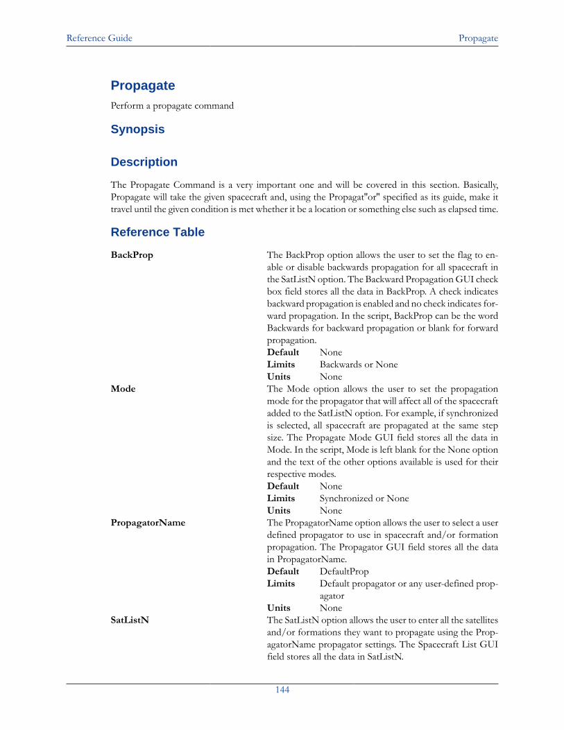
Reference Guide Propagate
144
PropagatePerform a propagate command
Synopsis
Description
The Propagate Command is a very important one and will be covered in this section. Basically,Propagate will take the given spacecraft and, using the Propagat''or'' specified as its guide, make ittravel until the given condition is met whether it be a location or something else such as elapsed time.
Reference Table
BackProp The BackProp option allows the user to set the flag to en-able or disable backwards propagation for all spacecraft inthe SatListN option. The Backward Propagation GUI checkbox field stores all the data in BackProp. A check indicatesbackward propagation is enabled and no check indicates for-ward propagation. In the script, BackProp can be the wordBackwards for backward propagation or blank for forwardpropagation.Default NoneLimits Backwards or NoneUnits None
Mode The Mode option allows the user to set the propagationmode for the propagator that will affect all of the spacecraftadded to the SatListN option. For example, if synchronizedis selected, all spacecraft are propagated at the same stepsize. The Propagate Mode GUI field stores all the data inMode. In the script, Mode is left blank for the None optionand the text of the other options available is used for theirrespective modes.Default NoneLimits Synchronized or NoneUnits None
PropagatorName The PropagatorName option allows the user to select a userdefined propagator to use in spacecraft and/or formationpropagation. The Propagator GUI field stores all the datain PropagatorName.Default DefaultPropLimits Default propagator or any user-defined prop-
agatorUnits None
SatListN The SatListN option allows the user to enter all the satellitesand/or formations they want to propagate using the Prop-agatorName propagator settings. The Spacecraft List GUIfield stores all the data in SatListN.
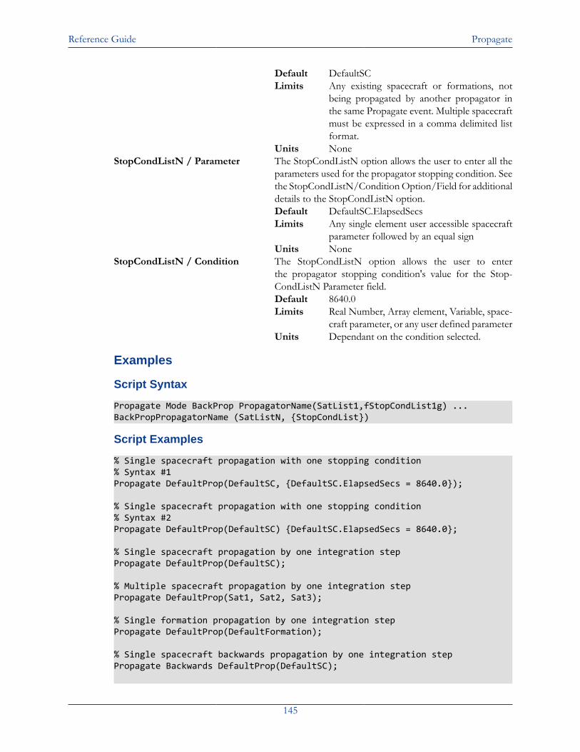
Reference Guide Propagate
145
Default DefaultSCLimits Any existing spacecraft or formations, not
being propagated by another propagator inthe same Propagate event. Multiple spacecraftmust be expressed in a comma delimited listformat.
Units NoneStopCondListN / Parameter The StopCondListN option allows the user to enter all the
parameters used for the propagator stopping condition. Seethe StopCondListN/Condition Option/Field for additionaldetails to the StopCondListN option.Default DefaultSC.ElapsedSecsLimits Any single element user accessible spacecraft
parameter followed by an equal signUnits None
StopCondListN / Condition The StopCondListN option allows the user to enterthe propagator stopping condition's value for the Stop-CondListN Parameter field.Default 8640.0Limits Real Number, Array element, Variable, space-
craft parameter, or any user defined parameterUnits Dependant on the condition selected.
Examples
Script Syntax
Propagate Mode BackProp PropagatorName(SatList1,fStopCondList1g) ...BackPropPropagatorName (SatListN, {StopCondList})
Script Examples
% Single spacecraft propagation with one stopping condition% Syntax #1Propagate DefaultProp(DefaultSC, {DefaultSC.ElapsedSecs = 8640.0});
% Single spacecraft propagation with one stopping condition% Syntax #2Propagate DefaultProp(DefaultSC) {DefaultSC.ElapsedSecs = 8640.0};
% Single spacecraft propagation by one integration stepPropagate DefaultProp(DefaultSC);
% Multiple spacecraft propagation by one integration stepPropagate DefaultProp(Sat1, Sat2, Sat3);
% Single formation propagation by one integration stepPropagate DefaultProp(DefaultFormation);
% Single spacecraft backwards propagation by one integration stepPropagate Backwards DefaultProp(DefaultSC);
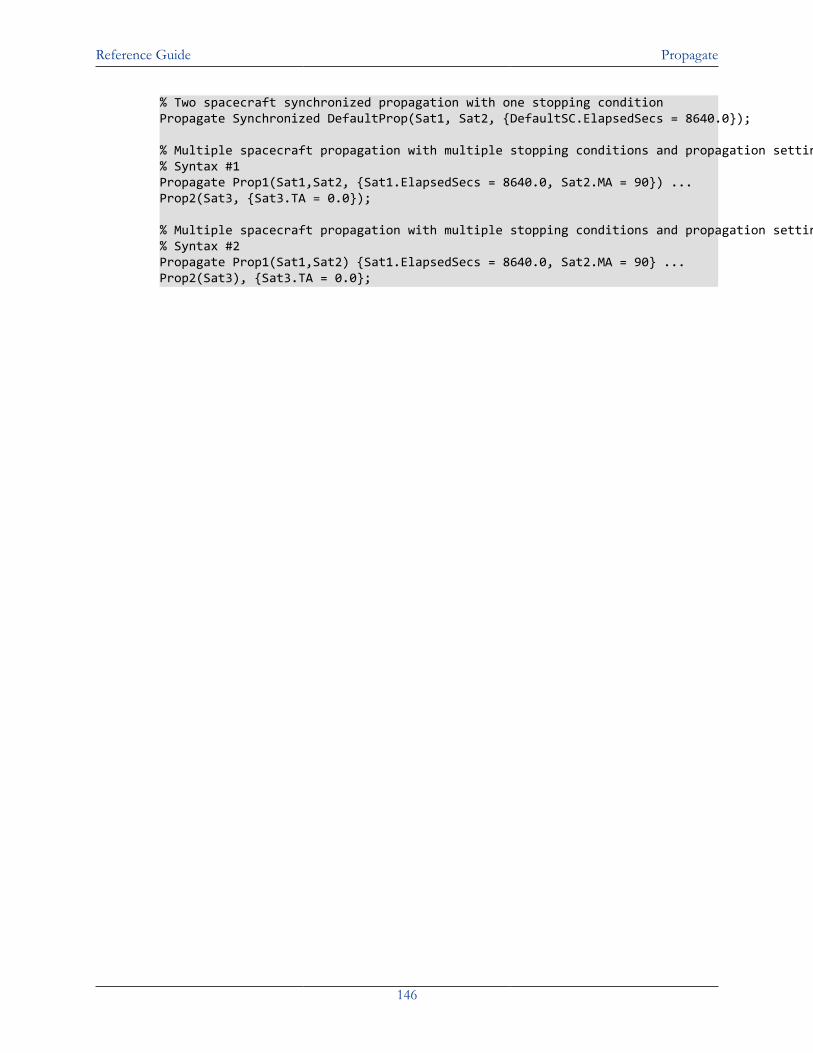
Reference Guide Propagate
146
% Two spacecraft synchronized propagation with one stopping conditionPropagate Synchronized DefaultProp(Sat1, Sat2, {DefaultSC.ElapsedSecs = 8640.0});
% Multiple spacecraft propagation with multiple stopping conditions and propagation settings% Syntax #1Propagate Prop1(Sat1,Sat2, {Sat1.ElapsedSecs = 8640.0, Sat2.MA = 90}) ...Prop2(Sat3, {Sat3.TA = 0.0});
% Multiple spacecraft propagation with multiple stopping conditions and propagation settings% Syntax #2Propagate Prop1(Sat1,Sat2) {Sat1.ElapsedSecs = 8640.0, Sat2.MA = 90} ...Prop2(Sat3), {Sat3.TA = 0.0};
Reference Guide Report
147
ReportOutput a report
Synopsis
Description
The report command allows the user find parameters of the orbit and the spacecraft at particularmoments in time. This command is inserted into the mission tree at various locations in the missiontree. The parameters found by this command are placed into a report file that can be accessed ata later time.
Options
ReportName The ReportName option allows the user to specift the ReportFile for data output.Default NoneLimits Any ReportFile createdUnits None
DataList The DataList option allows the user to output data to the Filename specified bythe ReportName. Multiple objects can be in the DataList when they are separatedby spaces.Default NoneLimits Spacecraft parameter, Array, Variable, String, or any other single user
defined parameterUnits None
Examples
Script Syntax
Report ReportName DataList
Script Examples
%Report the time and position of DefaultSC
Report DefaultReport DefaultSC.A1ModJulian DefaultSC.X DefaultSC.Y DefaultSC.Z;

Reference Guide Save
148
SaveUnder construction.
Synopsis
Under construction.
Under construction.
Under construction.
Examples
Script Syntax
Under construction.
Script Examples
Under construction.
Reference Guide SaveMission
149
SaveMissionSave the mission to an external file
Script Syntax
<incomplete>
Description
This reference page is incomplete at this time.
Reference Guide ScriptEvent
150
ScriptEventPerform a ScriptEvent command
Synopsis
Overview
The ScriptEvent command allows a user to enter in script within the GUI in the mission sequence.This can be useful in a number of ways if its easier to enter the script than to use the GUI inter-face. Also, if multiple things needed to be changed rapidly, this could be useful. Additionally, theScriptEvent allows a user to have more freedom if the GUI is problematic and won't allow the userto perform the desired operation.
Options
<Statements> Default NoneLimits Any valid line of GMAT scriptUnits None
Examples
Script Syntax
BeginScript <Statements>EndScript;
Script Examples
% Assignment Command inside Script Event
BeginScript GMAT testVar = 24;EndScript;
Reference Guide Stop
151
StopPerform a stop command
Synopsis
Description
The Stop command simply ends a mission in GMAT. Whether placed in the script or GUI, Stopwill halt the execution of the mission and have GMAT report back that the Command Sequencewas intentionally interrupted.
Examples
Script Syntax
Stop
Script Examples
% Stop between propagation sequencesPropagate DefaultProp(DefaultSC) DefaultSC.ElapsedSecs = 8640.0;Stop;Propagate DefaultProp(DefaultSC) DefaultSC.ElapsedDays = 10.0;
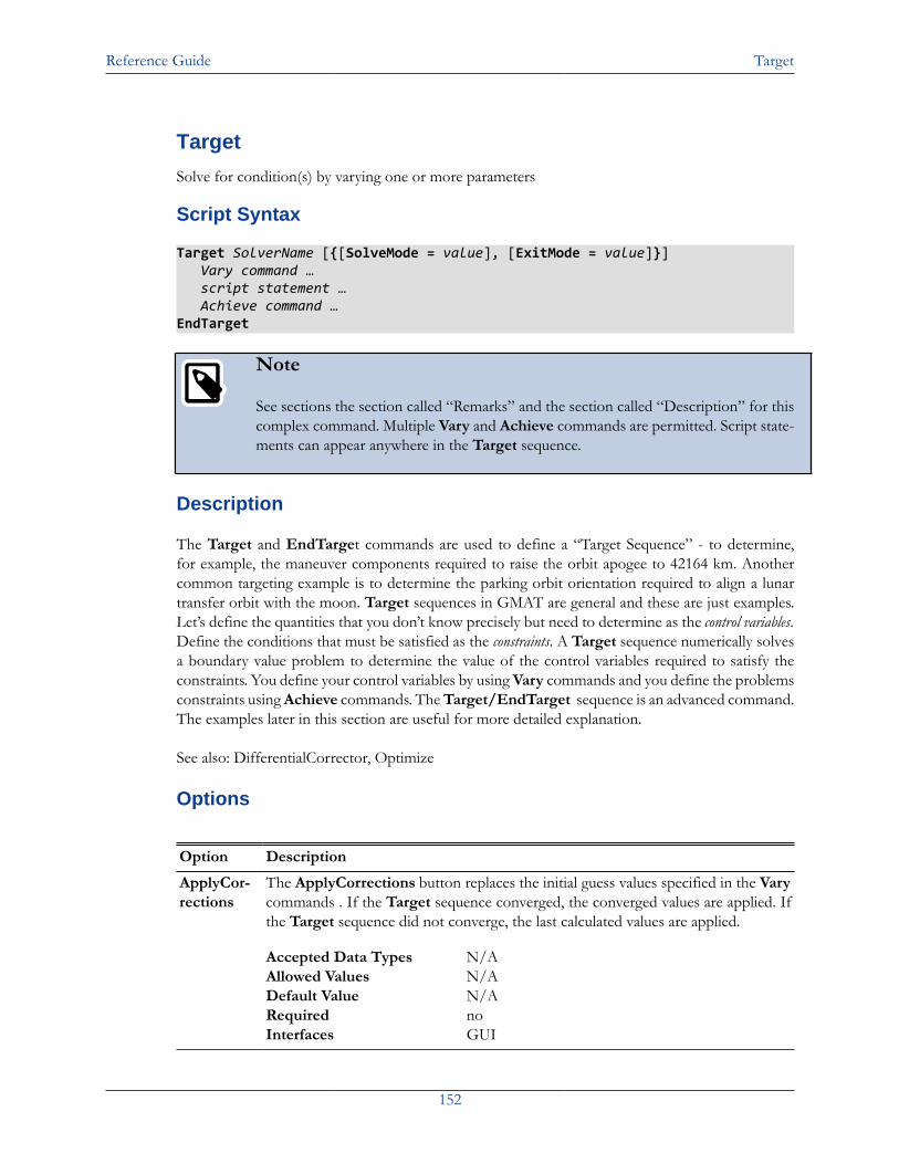
Reference Guide Target
152
Target
Solve for condition(s) by varying one or more parameters
Script Syntax
Target SolverName [{[SolveMode = value], [ExitMode = value]}] Vary command … script statement … Achieve command …EndTarget
Note
See sections the section called “Remarks” and the section called “Description” for thiscomplex command. Multiple Vary and Achieve commands are permitted. Script state-ments can appear anywhere in the Target sequence.
Description
The Target and EndTarget commands are used to define a “Target Sequence” - to determine,for example, the maneuver components required to raise the orbit apogee to 42164 km. Anothercommon targeting example is to determine the parking orbit orientation required to align a lunartransfer orbit with the moon. Target sequences in GMAT are general and these are just examples.Let’s define the quantities that you don’t know precisely but need to determine as the control variables.Define the conditions that must be satisfied as the constraints. A Target sequence numerically solvesa boundary value problem to determine the value of the control variables required to satisfy theconstraints. You define your control variables by using Vary commands and you define the problemsconstraints using Achieve commands. The Target/EndTarget sequence is an advanced command.The examples later in this section are useful for more detailed explanation.
See also: DifferentialCorrector, Optimize
Options
Option Description
ApplyCor-rections
The ApplyCorrections button replaces the initial guess values specified in the Varycommands . If the Target sequence converged, the converged values are applied. Ifthe Target sequence did not converge, the last calculated values are applied.
Accepted Data Types N/AAllowed Values N/ADefault Value N/ARequired noInterfaces GUI
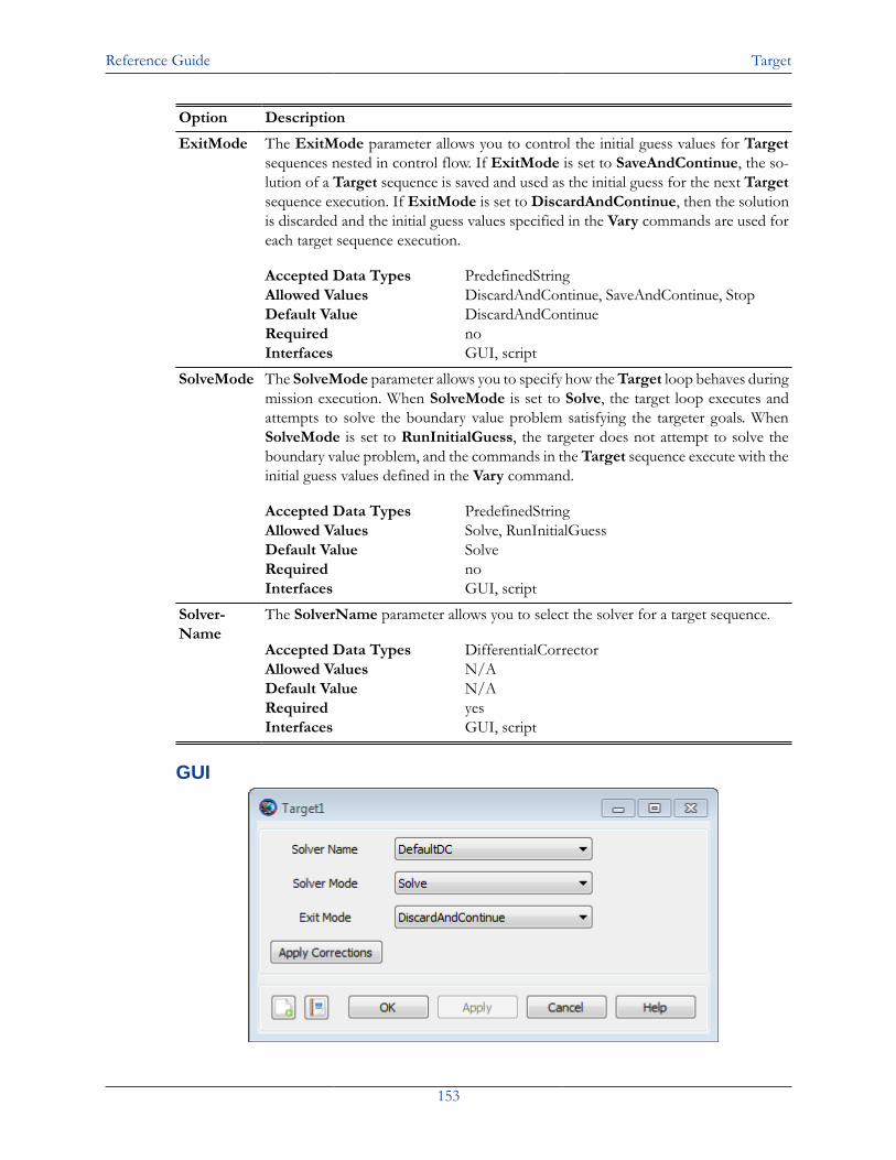
Reference Guide Target
153
Option Description
ExitMode The ExitMode parameter allows you to control the initial guess values for Targetsequences nested in control flow. If ExitMode is set to SaveAndContinue, the so-lution of a Target sequence is saved and used as the initial guess for the next Targetsequence execution. If ExitMode is set to DiscardAndContinue, then the solutionis discarded and the initial guess values specified in the Vary commands are used foreach target sequence execution.
Accepted Data Types PredefinedStringAllowed Values DiscardAndContinue, SaveAndContinue, StopDefault Value DiscardAndContinueRequired noInterfaces GUI, script
SolveMode The SolveMode parameter allows you to specify how the Target loop behaves duringmission execution. When SolveMode is set to Solve, the target loop executes andattempts to solve the boundary value problem satisfying the targeter goals. WhenSolveMode is set to RunInitialGuess, the targeter does not attempt to solve theboundary value problem, and the commands in the Target sequence execute with theinitial guess values defined in the Vary command.
Accepted Data Types PredefinedStringAllowed Values Solve, RunInitialGuessDefault Value SolveRequired noInterfaces GUI, script
Solver-Name
The SolverName parameter allows you to select the solver for a target sequence.
Accepted Data Types DifferentialCorrectorAllowed Values N/ADefault Value N/ARequired yesInterfaces GUI, script
GUI
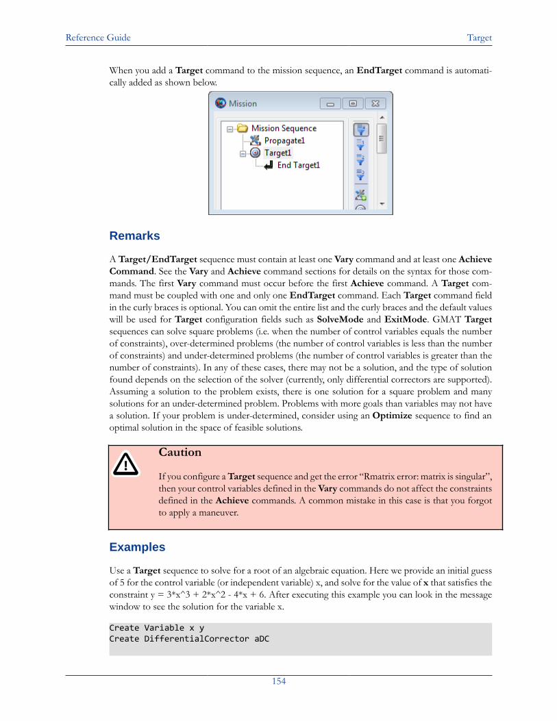
Reference Guide Target
154
When you add a Target command to the mission sequence, an EndTarget command is automati-cally added as shown below.
Remarks
A Target/EndTarget sequence must contain at least one Vary command and at least one AchieveCommand. See the Vary and Achieve command sections for details on the syntax for those com-mands. The first Vary command must occur before the first Achieve command. A Target com-mand must be coupled with one and only one EndTarget command. Each Target command fieldin the curly braces is optional. You can omit the entire list and the curly braces and the default valueswill be used for Target configuration fields such as SolveMode and ExitMode. GMAT Targetsequences can solve square problems (i.e. when the number of control variables equals the numberof constraints), over-determined problems (the number of control variables is less than the numberof constraints) and under-determined problems (the number of control variables is greater than thenumber of constraints). In any of these cases, there may not be a solution, and the type of solutionfound depends on the selection of the solver (currently, only differential correctors are supported).Assuming a solution to the problem exists, there is one solution for a square problem and manysolutions for an under-determined problem. Problems with more goals than variables may not havea solution. If your problem is under-determined, consider using an Optimize sequence to find anoptimal solution in the space of feasible solutions.
Caution
If you configure a Target sequence and get the error “Rmatrix error: matrix is singular”,then your control variables defined in the Vary commands do not affect the constraintsdefined in the Achieve commands. A common mistake in this case is that you forgotto apply a maneuver.
Examples
Use a Target sequence to solve for a root of an algebraic equation. Here we provide an initial guessof 5 for the control variable (or independent variable) x, and solve for the value of x that satisfies theconstraint y = 3*x^3 + 2*x^2 - 4*x + 6. After executing this example you can look in the messagewindow to see the solution for the variable x.
Create Variable x yCreate DifferentialCorrector aDC

Reference Guide Target
155
BeginMissionSequence
Target aDC Vary aDC(x = 5) y = 3*x^3 + 2*x^2 - 4*x + 6 Achieve aDC(y = 0)EndTarget
Use a Target sequence to raise orbit apogee. Here the control variable is the velocity componentof an ImpulsiveBurn object. The constraint is that the position vector magnitude at orbit apogeeis 42164 km.
Create Spacecraft aSatCreate Propagator aPropagatorCreate Variable ICreate ImpulsiveBurn aBurnCreate DifferentialCorrector aDC
Create OrbitView EarthViewEarthView.Add = {Earth,aSat}EarthView.ViewScaleFactor = 5
BeginMissionSequence
Target aDC Vary aDC(aBurn.Element1 = 1.0, {Upper = 3}) Maneuver aBurn(aSat) Propagate aPropagator(aSat,{aSat.Apoapsis}) Achieve aDC(aSat.RMAG = 42164)EndTarget
Reference Guide Toggle
156
TogglePerform a toggle command
Synopsis
Description
The Toggle command is useful in turning on/off certain plots so that they do not become unintel-ligible. They are particularly useful if a mission requires multiple sequences to fine-tune the answer.If this is the case, it might be better to turn off a plot until the final or second-to-last sequence sothat the rougher sequences don't obstruct the view of what is going on in the finesse sequences.
Options
OutputNames The Toggle option allows the user to assign the Plot/Report(s) to be toggled.When more than one Plot/Report is being toggled they need to be separatedby a space.Default DefaultOpenGLLimits Any OpenGL, Report, XYplot, or any other Plot/Report typeUnits None
Arg The Arg option allows the user to turn off or on the data output to a Plot/Report.Default OnLimits On or OffUnits None
Exmaples
Script Syntax
Toggle OutputNames Arg
Script Examples
% Turn off Report file for the first day of propagationToggle ReportFile1 OffPropagate DefaultProp(DefaultSC, {DefaultSC.ElapsedDays = 1});Toggle ReportFile1 OnPropagate DefaultProp(DefaultSC, {DefaultSC.ElapsedDays = 1});
% Turn off XYPlot and Report file for the first day of propagation Toggle XYPlot1 ReportFile1 OffPropagate DefaultProp(DefaultSC, {DefaultSC.ElapsedDays = 1});
Toggle XYPlot1 ReportFile1 OnPropagate DefaultProp(DefaultSC, {DefaultSC.ElapsedDays = 1})
Reference Guide Vary
157
VaryPerform a vary command
Synopsis
Description
The Vary command is used in conjunction with the Target and Optimize Commands. The Varycommand varies a particular parameter within the Target and Optimize Commands until certainconditions are met. It is a highly useful command for creating missions. Multiple Vary commandscan be used within the same targeting or optimizing sequence.
Options
Parameters Associated with All Solvers
SolverName The SolverName option allows the user to choose which solver to assign tothe vary command.Default DefaultDCLimits Any user defined solverUnits None
Variable The Variable option allows the user to select any single element user definedparameter, except a number, to vary. For example, DefaultIB.V, DefaultIB.N,DefaultIB.Element1, DefaultSC.TA, Array(1,1), and Variable are all valid val-ues. The three element burn vector or multidimensional Arrays are not validvalues.Default DefaultIB.VLimits Spacecrafy paremeter, Array element, Variable, or any other single
element user defined parameter, excluding numbersUnits None
InitialGuess The InitialGuess option allows the user to set the initial guess for the selectedVariable.Default 0.5Limits Real Number, Array element, Variable, or any user defined para-
meter that obeys the conditions for the selected Variable objectUnits km/s
Lower The Lower option allows the user to set Arg3 to the lower bound of the quantitybeing varied.Default 0.0Limits Real Number, Array element, Variable, or any user defined para-
meter (Upper > Lower )Units None
Upper The Upper option allows the user to set Arg4 to the upper bound of the quan-tity being varied.Default 3.14159Limits Real Number, Array element, Variable, or any user defined para-
meter (Upper > Lower )
Reference Guide Vary
158
Units None
Parameters Associated with Differential Corrector
Perturbation The Perturbation option is set by specifying a value for Arg1. The value ofArg1 is the perturbation size in calculating the finite difference derivative.Default 1e-4Limits Real Number, Array element, Variable, or any user defined para-
meter > 0Units None
MaxStep The MaxStep option is set by specifying a value for Arg2. The value of Arg2limits the size of the step taken during an interaction of the differential cor-rector.Default 0.2Limits Real Number, Array element, Variable, or any user defined para-
meter > 0Units None
Parameters Associated with fmincon Optimizer
Additive Scale Factor The AdditiveScaleFactor Field is used to nondimensionalizethe independent variable. fmincon sees only the nondimen-sional form of the variable. The nondimensionalization isperformed using the following equation: xn = (xd - a)/m .(xn is the non-dimensional parameter. xd is the dimensionalparameter. a= additive scale factor. m= multiplicative scalefactor.)Default 0Limits Real Number, Array element, Variable, or any
user defined parameterUnits None
Multiplicative Scale Factor The MultiplicativeScaleFactor Field is used to nondimen-sionalize the independent variable. fmincon sees only thenondimensional form of the variable. The nondimension-alization is performed using the following equation: xn =(xd - a)/m . (xn is the non-dimensional parameter. xd is thedimensional parameter. a= additive scale factor. m= multi-plicative scale factor.)Default 1.0Limits Real Number, Array element, Variable, or any
user defined parameterUnits None
Examples
Script Syntax
Vary SolverName(Variable=InitialGuess,{Perturbation=Arg1, MaxStep=Arg2, Lower=Arg3,...Upper=Arg4, AdditiveScalefactor=Arg6,MultiplicativeScalefactor=Arg6})
Reference Guide Vary
159
Script Examples
% Impulsive Burn Vary Command
Vary DefaultDC(DefaultIB.V = 0.5, {Perturbation = 0.0001, MaxStep = 0.2, Lower = 0, Upper = 3.14159});
Reference Guide While
160
While
Run a while loop
Synopsis
Description
The while loop is a control logic function that allows GMAT to check the spacecraft's status on agiven parameter while performing a command or another control logic function within the missionsequence. When a spacecraft has reached the given property, the while loop will check its conditionand react according to the equation defined in the loop's dialog box.
Options
<logical expression> Arg1 and Arg2 can be any of the following: Real Number, Array,Variable, Spacecraft Parameter or any other user defined parame-ter.Default DefaultSC.ElapsedDays < 1.0Limits Arg1 < Arg2 and < can be > , < , >= , <= , == , ~=Units None
<Statements> Default NoneLimits Any script line that can be in the mission sequenceUnits None
| The | option allows the user to set an OR operator in between s.Default NoneLimits NoneUnits None
& The & option allows the user to set an AND operator in between<logical expression>s.Default NoneLimits NoneUnits None
Examples
Script Syntax
• Simple While Loop
While <logical expression>; <Statements>;EndWhile;
• Compound While Loop
While <logical expression> | <logical expression> & <logical expression>; <Statements>EndWhile;
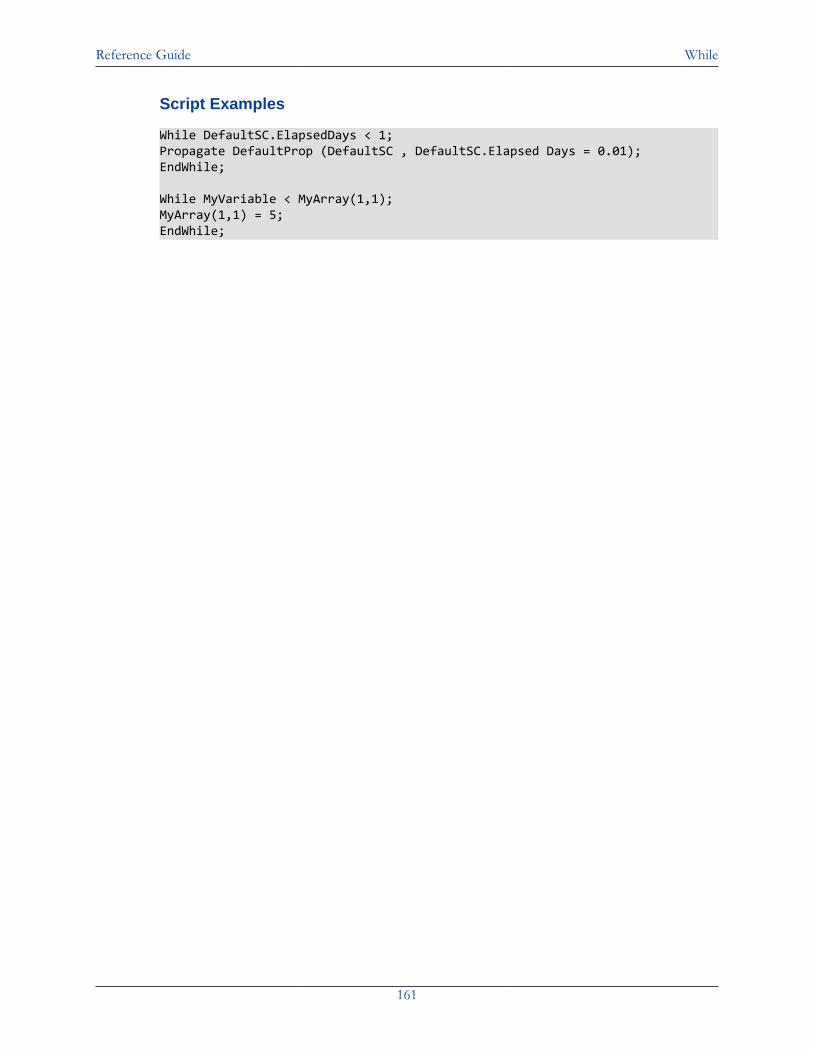
Reference Guide While
161
Script Examples
While DefaultSC.ElapsedDays < 1;Propagate DefaultProp (DefaultSC , DefaultSC.Elapsed Days = 0.01);EndWhile;
While MyVariable < MyArray(1,1);MyArray(1,1) = 5;EndWhile;
Part VI. Release Notes
Table of ContentsGMAT R2011a Release Notes ........................................................................................................ 163
New Features ........................................................................................................................ 163Improvements ....................................................................................................................... 166Compatibility Changes ........................................................................................................... 168Fixed Issues .......................................................................................................................... 170Known Issues ....................................................................................................................... 170
GMAT R2012a Release Notes ........................................................................................................ 174New Features ........................................................................................................................ 174Improvements ....................................................................................................................... 176Compatibility Changes ........................................................................................................... 179Known & Fixed Issues .......................................................................................................... 180
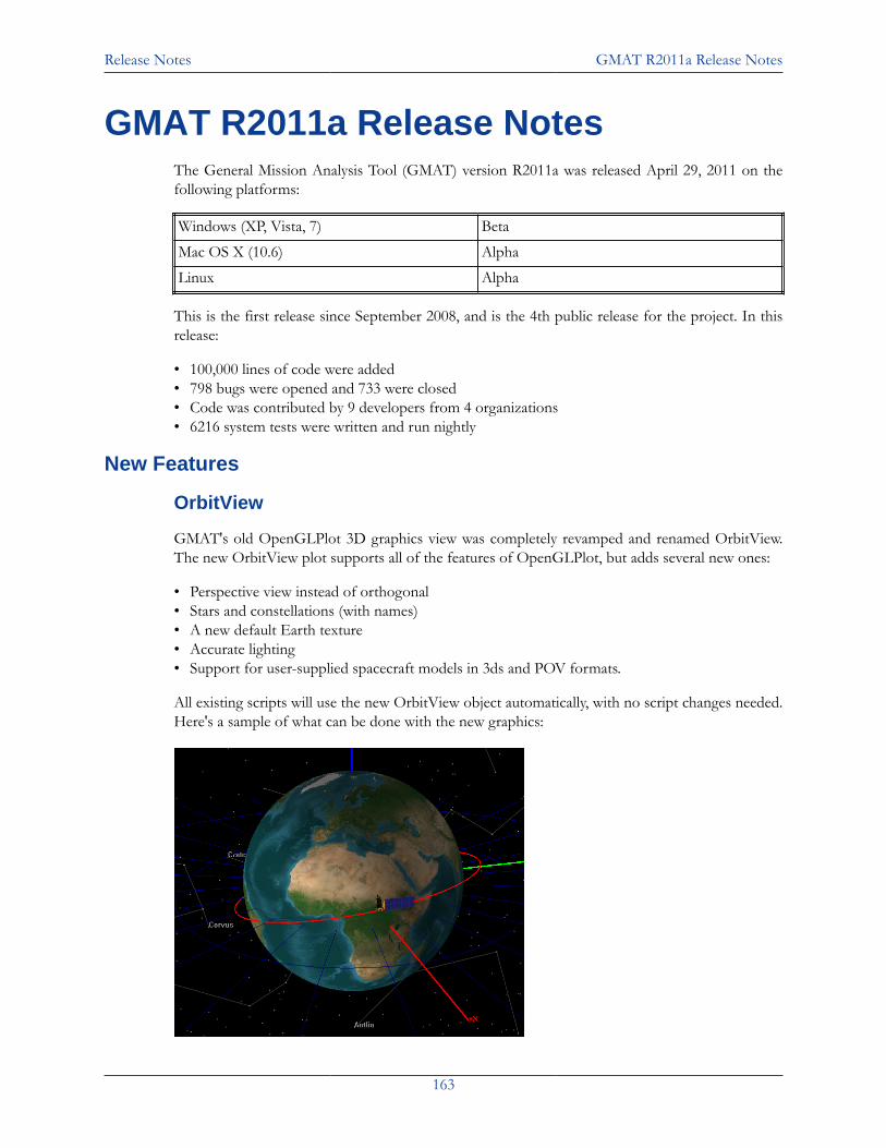
Release Notes GMAT R2011a Release Notes
163
GMAT R2011a Release NotesThe General Mission Analysis Tool (GMAT) version R2011a was released April 29, 2011 on thefollowing platforms:
Windows (XP, Vista, 7) Beta
Mac OS X (10.6) Alpha
Linux Alpha
This is the first release since September 2008, and is the 4th public release for the project. In thisrelease:
• 100,000 lines of code were added• 798 bugs were opened and 733 were closed• Code was contributed by 9 developers from 4 organizations• 6216 system tests were written and run nightly
New Features
OrbitView
GMAT's old OpenGLPlot 3D graphics view was completely revamped and renamed OrbitView.The new OrbitView plot supports all of the features of OpenGLPlot, but adds several new ones:
• Perspective view instead of orthogonal• Stars and constellations (with names)• A new default Earth texture• Accurate lighting• Support for user-supplied spacecraft models in 3ds and POV formats.
All existing scripts will use the new OrbitView object automatically, with no script changes needed.Here's a sample of what can be done with the new graphics:
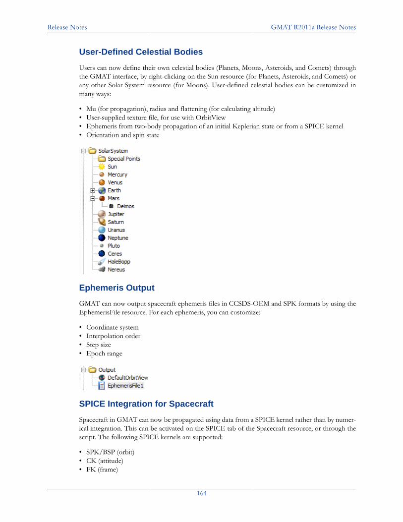
Release Notes GMAT R2011a Release Notes
164
User-Defined Celestial Bodies
Users can now define their own celestial bodies (Planets, Moons, Asteroids, and Comets) throughthe GMAT interface, by right-clicking on the Sun resource (for Planets, Asteroids, and Comets) orany other Solar System resource (for Moons). User-defined celestial bodies can be customized inmany ways:
• Mu (for propagation), radius and flattening (for calculating altitude)• User-supplied texture file, for use with OrbitView• Ephemeris from two-body propagation of an initial Keplerian state or from a SPICE kernel• Orientation and spin state
Ephemeris Output
GMAT can now output spacecraft ephemeris files in CCSDS-OEM and SPK formats by using theEphemerisFile resource. For each ephemeris, you can customize:
• Coordinate system• Interpolation order• Step size• Epoch range
SPICE Integration for Spacecraft
Spacecraft in GMAT can now be propagated using data from a SPICE kernel rather than by numer-ical integration. This can be activated on the SPICE tab of the Spacecraft resource, or through thescript. The following SPICE kernels are supported:
• SPK/BSP (orbit)• CK (attitude)• FK (frame)
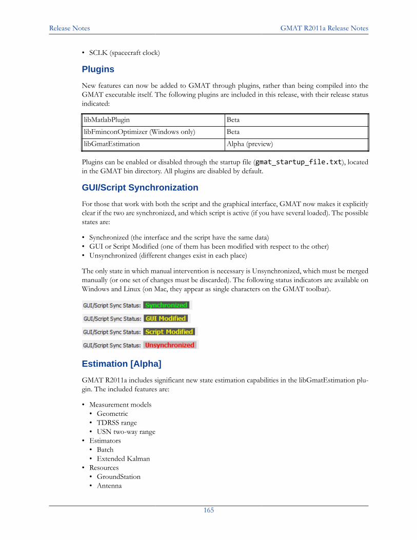
Release Notes GMAT R2011a Release Notes
165
• SCLK (spacecraft clock)
Plugins
New features can now be added to GMAT through plugins, rather than being compiled into theGMAT executable itself. The following plugins are included in this release, with their release statusindicated:
libMatlabPlugin Beta
libFminconOptimizer (Windows only) Beta
libGmatEstimation Alpha (preview)
Plugins can be enabled or disabled through the startup file (gmat_startup_file.txt), locatedin the GMAT bin directory. All plugins are disabled by default.
GUI/Script Synchronization
For those that work with both the script and the graphical interface, GMAT now makes it explicitlyclear if the two are synchronized, and which script is active (if you have several loaded). The possiblestates are:
• Synchronized (the interface and the script have the same data)• GUI or Script Modified (one of them has been modified with respect to the other)• Unsynchronized (different changes exist in each place)
The only state in which manual intervention is necessary is Unsynchronized, which must be mergedmanually (or one set of changes must be discarded). The following status indicators are available onWindows and Linux (on Mac, they appear as single characters on the GMAT toolbar).
Estimation [Alpha]
GMAT R2011a includes significant new state estimation capabilities in the libGmatEstimation plu-gin. The included features are:
• Measurement models• Geometric• TDRSS range• USN two-way range
• Estimators• Batch• Extended Kalman
• Resources• GroundStation• Antenna
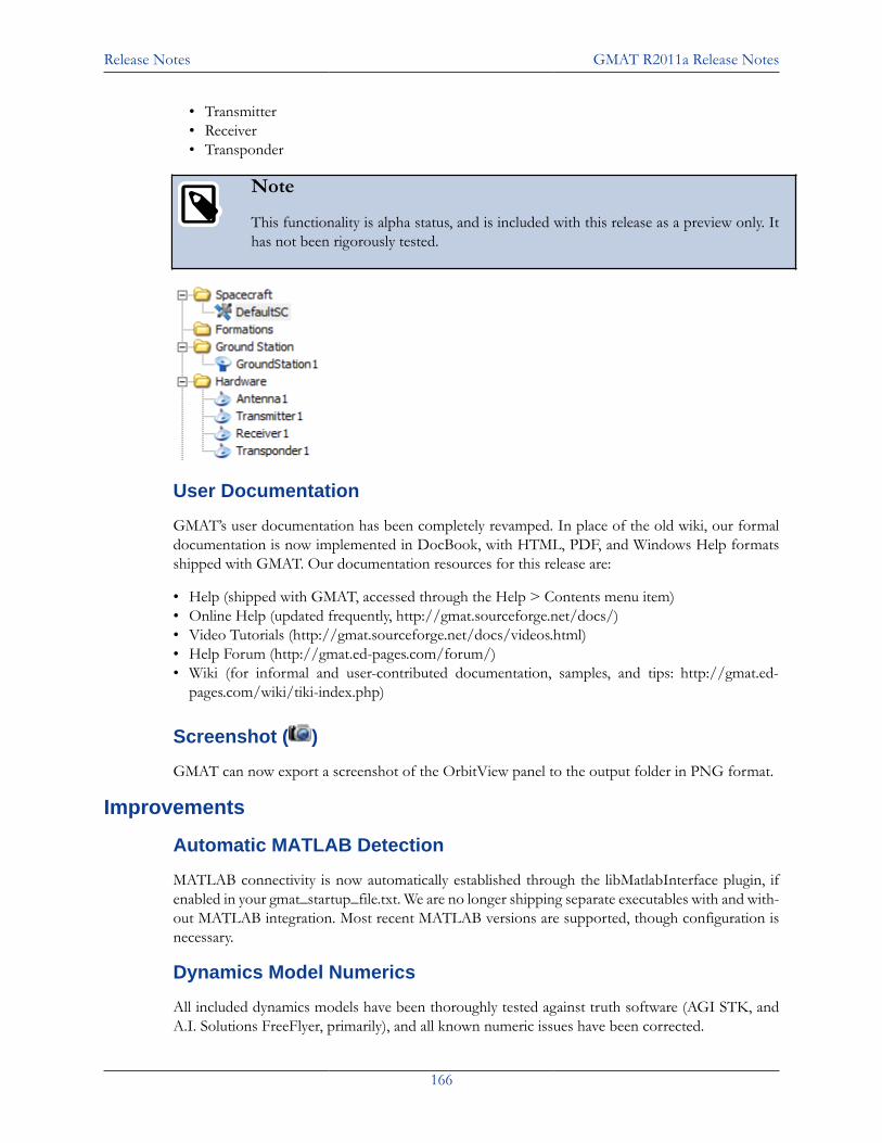
Release Notes GMAT R2011a Release Notes
166
• Transmitter• Receiver• Transponder
Note
This functionality is alpha status, and is included with this release as a preview only. Ithas not been rigorously tested.
User Documentation
GMAT’s user documentation has been completely revamped. In place of the old wiki, our formaldocumentation is now implemented in DocBook, with HTML, PDF, and Windows Help formatsshipped with GMAT. Our documentation resources for this release are:
• Help (shipped with GMAT, accessed through the Help > Contents menu item)• Online Help (updated frequently, http://gmat.sourceforge.net/docs/)• Video Tutorials (http://gmat.sourceforge.net/docs/videos.html)• Help Forum (http://gmat.ed-pages.com/forum/)• Wiki (for informal and user-contributed documentation, samples, and tips: http://gmat.ed-
pages.com/wiki/tiki-index.php)
Screenshot ( )
GMAT can now export a screenshot of the OrbitView panel to the output folder in PNG format.
Improvements
Automatic MATLAB Detection
MATLAB connectivity is now automatically established through the libMatlabInterface plugin, ifenabled in your gmat_startup_file.txt. We are no longer shipping separate executables with and with-out MATLAB integration. Most recent MATLAB versions are supported, though configuration isnecessary.
Dynamics Model Numerics
All included dynamics models have been thoroughly tested against truth software (AGI STK, andA.I. Solutions FreeFlyer, primarily), and all known numeric issues have been corrected.
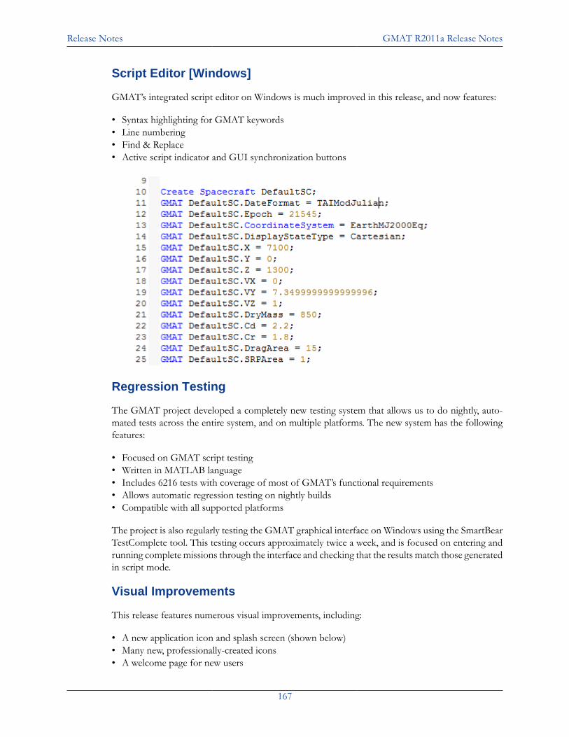
Release Notes GMAT R2011a Release Notes
167
Script Editor [Windows]
GMAT’s integrated script editor on Windows is much improved in this release, and now features:
• Syntax highlighting for GMAT keywords• Line numbering• Find & Replace• Active script indicator and GUI synchronization buttons
Regression Testing
The GMAT project developed a completely new testing system that allows us to do nightly, auto-mated tests across the entire system, and on multiple platforms. The new system has the followingfeatures:
• Focused on GMAT script testing• Written in MATLAB language• Includes 6216 tests with coverage of most of GMAT’s functional requirements• Allows automatic regression testing on nightly builds• Compatible with all supported platforms
The project is also regularly testing the GMAT graphical interface on Windows using the SmartBearTestComplete tool. This testing occurs approximately twice a week, and is focused on entering andrunning complete missions through the interface and checking that the results match those generatedin script mode.
Visual Improvements
This release features numerous visual improvements, including:
• A new application icon and splash screen (shown below)• Many new, professionally-created icons• A welcome page for new users
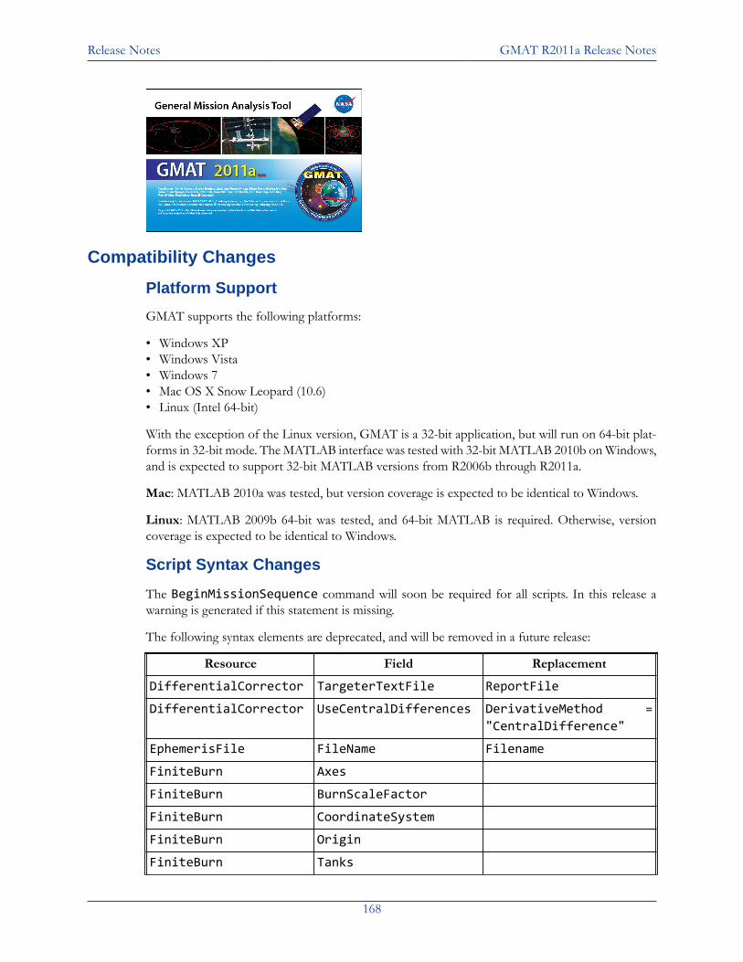
Release Notes GMAT R2011a Release Notes
168
Compatibility Changes
Platform Support
GMAT supports the following platforms:
• Windows XP• Windows Vista• Windows 7• Mac OS X Snow Leopard (10.6)• Linux (Intel 64-bit)
With the exception of the Linux version, GMAT is a 32-bit application, but will run on 64-bit plat-forms in 32-bit mode. The MATLAB interface was tested with 32-bit MATLAB 2010b on Windows,and is expected to support 32-bit MATLAB versions from R2006b through R2011a.
Mac: MATLAB 2010a was tested, but version coverage is expected to be identical to Windows.
Linux: MATLAB 2009b 64-bit was tested, and 64-bit MATLAB is required. Otherwise, versioncoverage is expected to be identical to Windows.
Script Syntax Changes
The BeginMissionSequence command will soon be required for all scripts. In this release awarning is generated if this statement is missing.
The following syntax elements are deprecated, and will be removed in a future release:
Resource Field Replacement
DifferentialCorrector TargeterTextFile ReportFile
DifferentialCorrector UseCentralDifferences DerivativeMethod ="CentralDifference"
EphemerisFile FileName Filename
FiniteBurn Axes
FiniteBurn BurnScaleFactor
FiniteBurn CoordinateSystem
FiniteBurn Origin
FiniteBurn Tanks
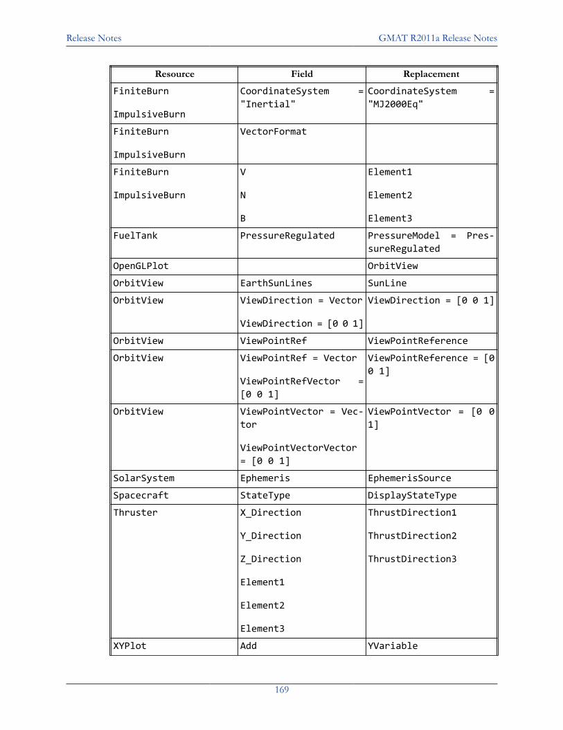
Release Notes GMAT R2011a Release Notes
169
Resource Field Replacement
FiniteBurn
ImpulsiveBurn
CoordinateSystem ="Inertial"
CoordinateSystem ="MJ2000Eq"
FiniteBurn
ImpulsiveBurn
VectorFormat
FiniteBurn
ImpulsiveBurn
V
N
B
Element1
Element2
Element3
FuelTank PressureRegulated PressureModel = Pres-sureRegulated
OpenGLPlot OrbitView
OrbitView EarthSunLines SunLine
OrbitView ViewDirection = Vector
ViewDirection = [0 0 1]
ViewDirection = [0 0 1]
OrbitView ViewPointRef ViewPointReference
OrbitView ViewPointRef = Vector
ViewPointRefVector =[0 0 1]
ViewPointReference = [00 1]
OrbitView ViewPointVector = Vec-tor
ViewPointVectorVector= [0 0 1]
ViewPointVector = [0 01]
SolarSystem Ephemeris EphemerisSource
Spacecraft StateType DisplayStateType
Thruster X_Direction
Y_Direction
Z_Direction
Element1
Element2
Element3
ThrustDirection1
ThrustDirection2
ThrustDirection3
XYPlot Add YVariable
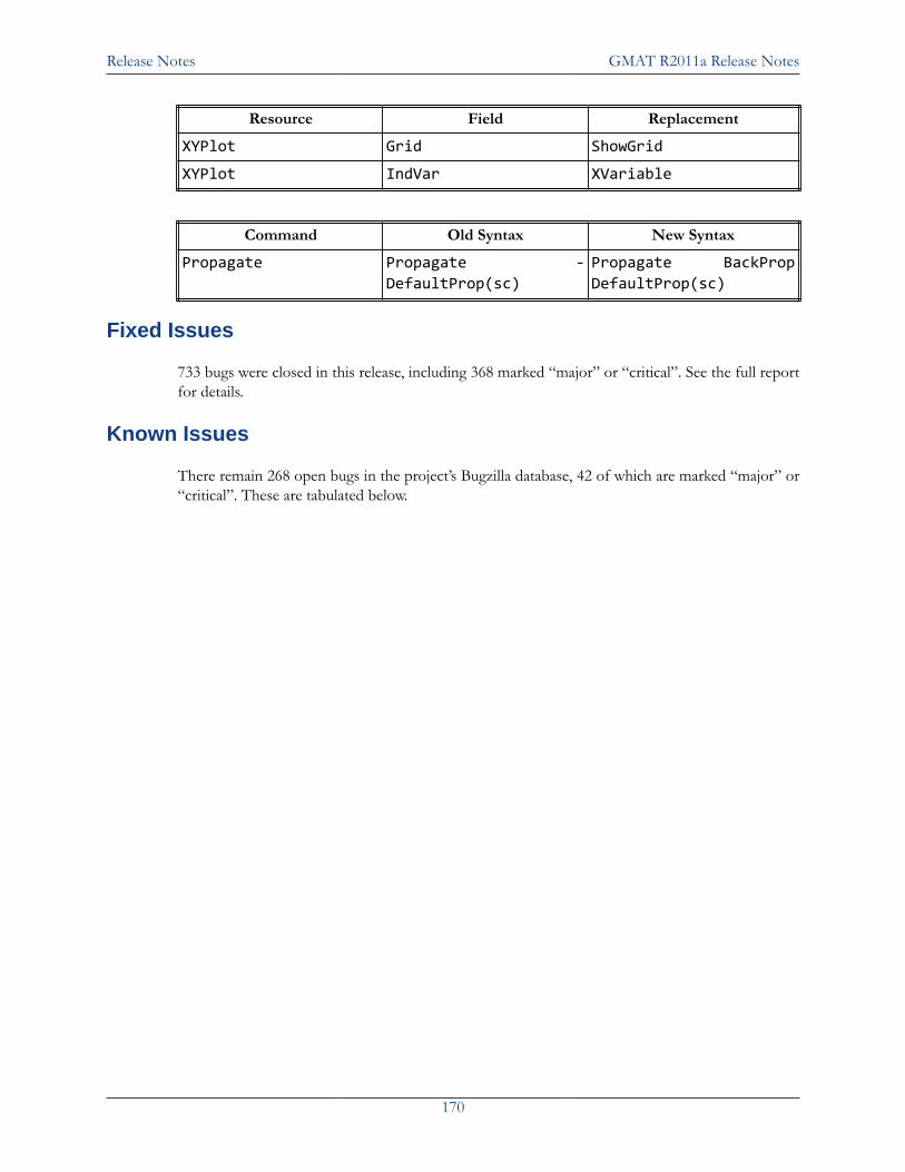
Release Notes GMAT R2011a Release Notes
170
Resource Field Replacement
XYPlot Grid ShowGrid
XYPlot IndVar XVariable
Command Old Syntax New Syntax
Propagate Propagate -DefaultProp(sc)
Propagate BackPropDefaultProp(sc)
Fixed Issues
733 bugs were closed in this release, including 368 marked “major” or “critical”. See the full reportfor details.
Known Issues
There remain 268 open bugs in the project’s Bugzilla database, 42 of which are marked “major” or“critical”. These are tabulated below.
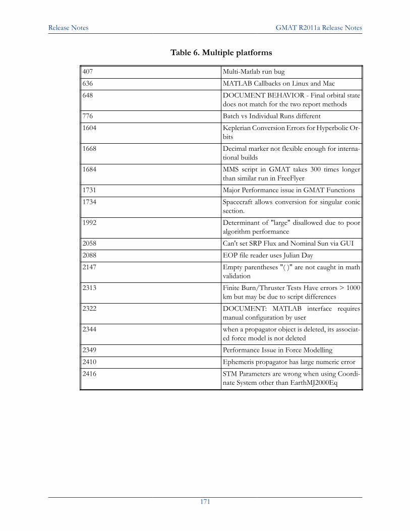
Release Notes GMAT R2011a Release Notes
171
Table 6. Multiple platforms
407 Multi-Matlab run bug
636 MATLAB Callbacks on Linux and Mac
648 DOCUMENT BEHAVIOR - Final orbital statedoes not match for the two report methods
776 Batch vs Individual Runs different
1604 Keplerian Conversion Errors for Hyperbolic Or-bits
1668 Decimal marker not flexible enough for interna-tional builds
1684 MMS script in GMAT takes 300 times longerthan similar run in FreeFlyer
1731 Major Performance issue in GMAT Functions
1734 Spacecraft allows conversion for singular conicsection.
1992 Determinant of "large" disallowed due to pooralgorithm performance
2058 Can't set SRP Flux and Nominal Sun via GUI
2088 EOP file reader uses Julian Day
2147 Empty parentheses "( )" are not caught in mathvalidation
2313 Finite Burn/Thruster Tests Have errors > 1000km but may be due to script differences
2322 DOCUMENT: MATLAB interface requiresmanual configuration by user
2344 when a propagator object is deleted, its associat-ed force model is not deleted
2349 Performance Issue in Force Modelling
2410 Ephemeris propagator has large numeric error
2416 STM Parameters are wrong when using Coordi-nate System other than EarthMJ2000Eq
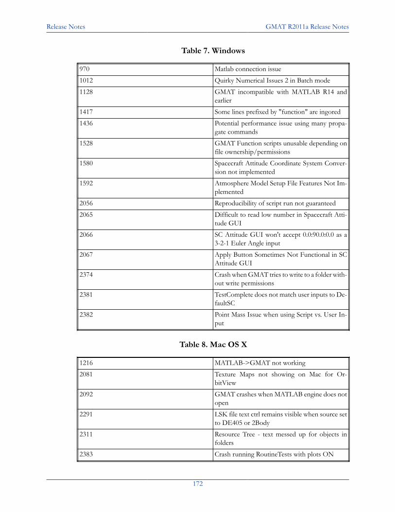
Release Notes GMAT R2011a Release Notes
172
Table 7. Windows
970 Matlab connection issue
1012 Quirky Numerical Issues 2 in Batch mode
1128 GMAT incompatible with MATLAB R14 andearlier
1417 Some lines prefixed by "function" are ingored
1436 Potential performance issue using many propa-gate commands
1528 GMAT Function scripts unusable depending onfile ownership/permissions
1580 Spacecraft Attitude Coordinate System Conver-sion not implemented
1592 Atmosphere Model Setup File Features Not Im-plemented
2056 Reproducibility of script run not guaranteed
2065 Difficult to read low number in Spacecraft Atti-tude GUI
2066 SC Attitude GUI won't accept 0.0:90.0:0.0 as a3-2-1 Euler Angle input
2067 Apply Button Sometimes Not Functional in SCAttitude GUI
2374 Crash when GMAT tries to write to a folder with-out write permissions
2381 TestComplete does not match user inputs to De-faultSC
2382 Point Mass Issue when using Script vs. User In-put
Table 8. Mac OS X
1216 MATLAB->GMAT not working
2081 Texture Maps not showing on Mac for Or-bitView
2092 GMAT crashes when MATLAB engine does notopen
2291 LSK file text ctrl remains visible when source setto DE405 or 2Body
2311 Resource Tree - text messed up for objects infolders
2383 Crash running RoutineTests with plots ON

Release Notes GMAT R2011a Release Notes
173
Table 9. Linux
1851 On Linux, STC Editor crashes GMAT on Close
1877 On Linux, Ctrl-C crashes GMAT if no MDIChil-dren are open
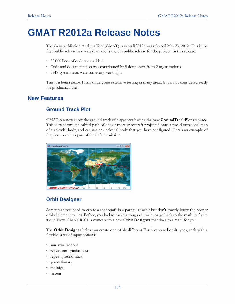
Release Notes GMAT R2012a Release Notes
174
GMAT R2012a Release NotesThe General Mission Analysis Tool (GMAT) version R2012a was released May 23, 2012. This is thefirst public release in over a year, and is the 5th public release for the project. In this release:
• 52,000 lines of code were added• Code and documentation was contributed by 9 developers from 2 organizations• 6847 system tests were run every weeknight
This is a beta release. It has undergone extensive testing in many areas, but is not considered readyfor production use.
New Features
Ground Track Plot
GMAT can now show the ground track of a spacecraft using the new GroundTrackPlot resource.This view shows the orbital path of one or more spacecraft projected onto a two-dimensional mapof a celestial body, and can use any celestial body that you have configured. Here's an example ofthe plot created as part of the default mission:
Orbit Designer
Sometimes you need to create a spacecraft in a particular orbit but don't exactly know the properorbital element values. Before, you had to make a rough estimate, or go back to the math to figureit out. Now, GMAT R2012a comes with a new Orbit Designer that does this math for you.
The Orbit Designer helps you create one of six different Earth-centered orbit types, each with aflexible array of input options:
• sun-synchronous• repeat sun-synchronous• repeat ground track• geostationary• molniya• frozen
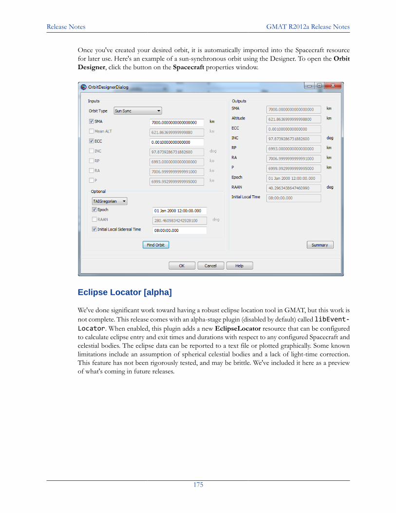
Release Notes GMAT R2012a Release Notes
175
Once you've created your desired orbit, it is automatically imported into the Spacecraft resourcefor later use. Here's an example of a sun-synchronous orbit using the Designer. To open the OrbitDesigner, click the button on the Spacecraft properties window.
Eclipse Locator [alpha]
We've done significant work toward having a robust eclipse location tool in GMAT, but this work isnot complete. This release comes with an alpha-stage plugin (disabled by default) called libEvent-Locator. When enabled, this plugin adds a new EclipseLocator resource that can be configuredto calculate eclipse entry and exit times and durations with respect to any configured Spacecraft andcelestial bodies. The eclipse data can be reported to a text file or plotted graphically. Some knownlimitations include an assumption of spherical celestial bodies and a lack of light-time correction.This feature has not been rigorously tested, and may be brittle. We've included it here as a previewof what's coming in future releases.
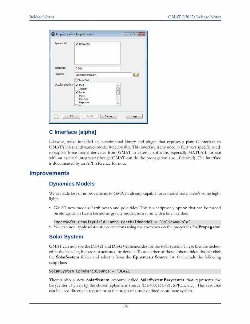
Release Notes GMAT R2012a Release Notes
176
C Interface [alpha]
Likewise, we've included an experimental library and plugin that exposes a plain-C interface toGMAT's internal dynamics model functionality. This interface is intended to fill a very specific need:to expose force model derivates from GMAT to external software, especially MATLAB, for usewith an external integrator (though GMAT can do the propagation also, if desired). The interfaceis documented by an API reference for now.
Improvements
Dynamics Models
We've made lots of improvements to GMAT's already capable force model suite. Here's some high-lights:
• GMAT now models Earth ocean and pole tides. This is a script-only option that can be turnedon alongside an Earth harmonic gravity model; turn it on with a line like this:
ForceModel.GravityField.Earth.EarthTideModel = 'SolidAndPole'• You can now apply relativistic corrections using the checkbox on the properties for Propagator.
Solar System
GMAT can now use the DE421 and DE424 ephemerides for the solar system. These files are includ-ed in the installer, but are not activated by default. To use either of these ephemerides, double-clickthe SolarSystem folder and select it from the Ephemeris Source list. Or include the followingscript line:
SolarSystem.EphemerisSource = 'DE421'
There's also a new SolarSystem resource called SolarSystemBarycenter that represents thebarycenter as given by the chosen ephemeris source (DE405, DE421, SPICE, etc.). This resourcecan be used directly in reports or as the origin of a user-defined coordinate system.
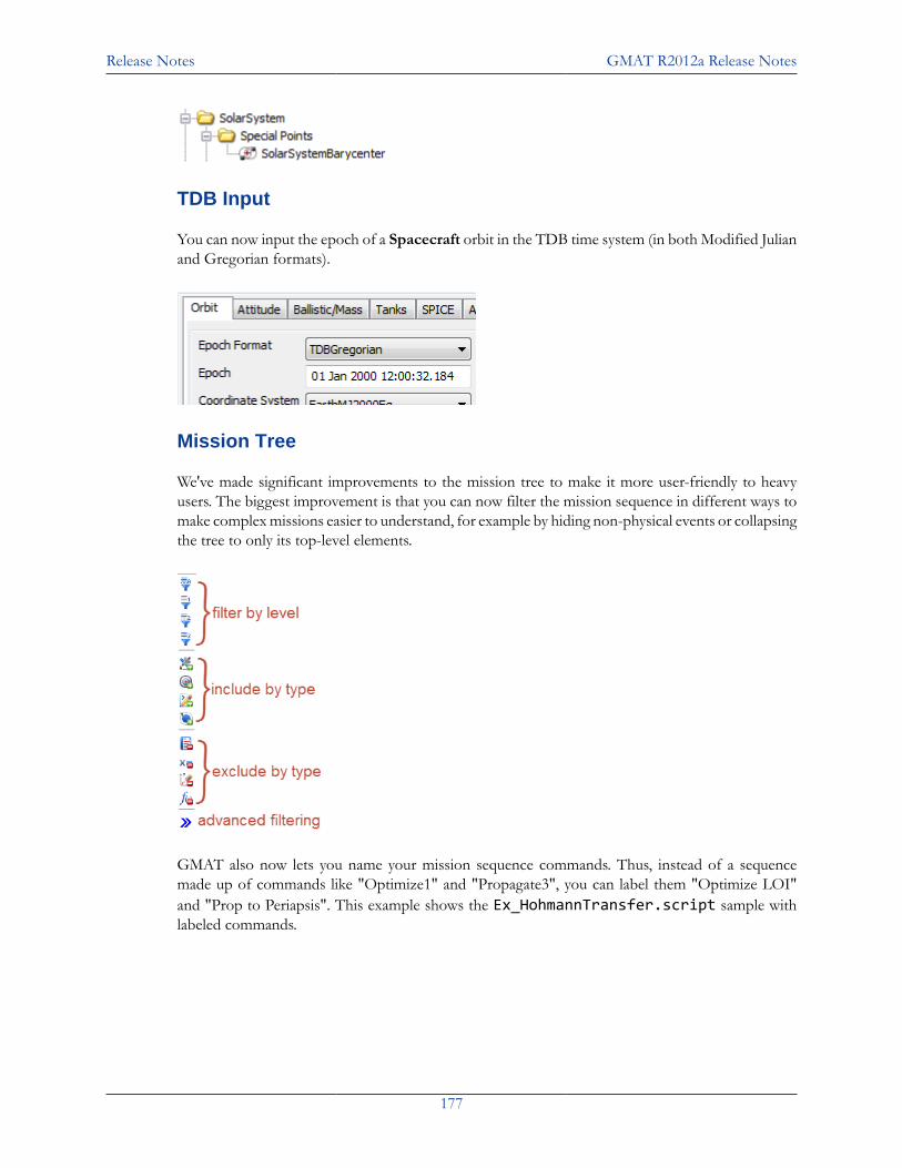
Release Notes GMAT R2012a Release Notes
177
TDB Input
You can now input the epoch of a Spacecraft orbit in the TDB time system (in both Modified Julianand Gregorian formats).
Mission Tree
We've made significant improvements to the mission tree to make it more user-friendly to heavyusers. The biggest improvement is that you can now filter the mission sequence in different ways tomake complex missions easier to understand, for example by hiding non-physical events or collapsingthe tree to only its top-level elements.
GMAT also now lets you name your mission sequence commands. Thus, instead of a sequencemade up of commands like "Optimize1" and "Propagate3", you can label them "Optimize LOI"and "Prop to Periapsis". This example shows the Ex_HohmannTransfer.script sample withlabeled commands.
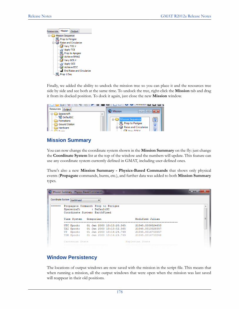
Release Notes GMAT R2012a Release Notes
178
Finally, we added the ability to undock the mission tree so you can place it and the resources treeside by side and see both at the same time. To undock the tree, right-click the Mission tab and dragit from its docked position. To dock it again, just close the new Mission window.
Mission Summary
You can now change the coordinate system shown in the Mission Summary on the fly: just changethe Coordinate System list at the top of the window and the numbers will update. This feature canuse any coordinate system currently defined in GMAT, including user-defined ones.
There's also a new Mission Summary - Physics-Based Commands that shows only physicalevents (Propagate commands, burns, etc.), and further data was added to both Mission Summarytypes.
Window Persistency
The locations of output windows are now saved with the mission in the script file. This means thatwhen running a mission, all the output windows that were open when the mission was last savedwill reappear in their old positions.
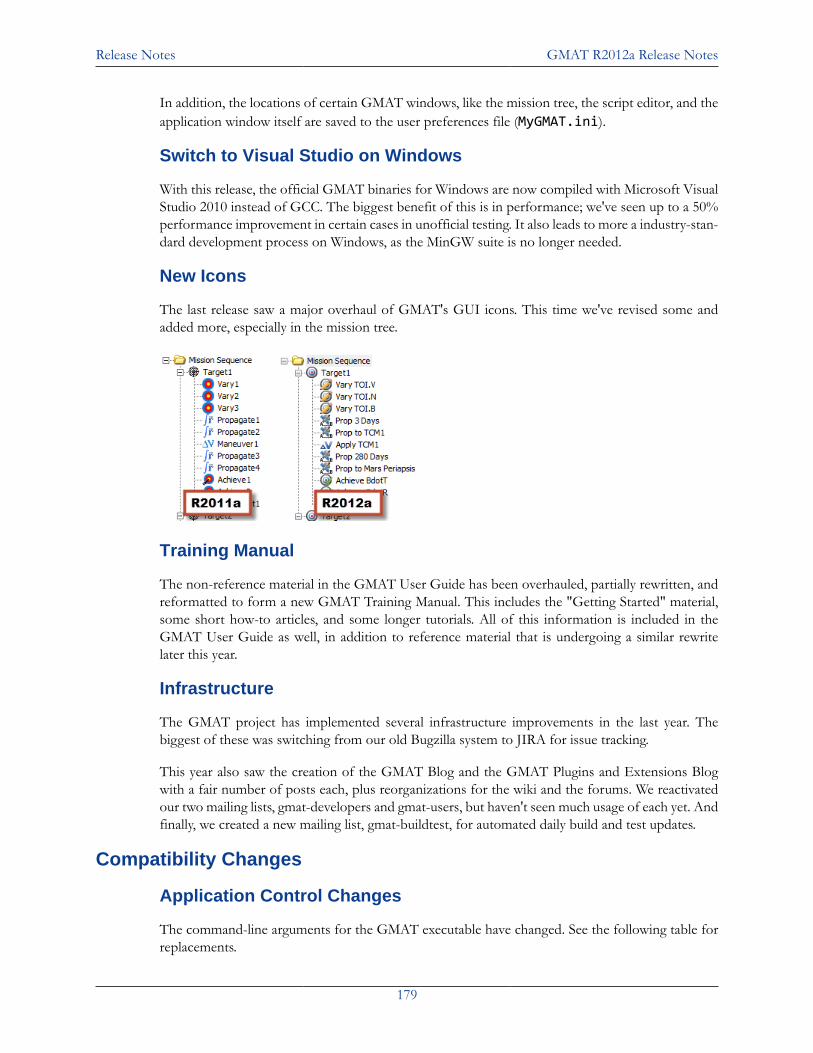
Release Notes GMAT R2012a Release Notes
179
In addition, the locations of certain GMAT windows, like the mission tree, the script editor, and theapplication window itself are saved to the user preferences file (MyGMAT.ini).
Switch to Visual Studio on Windows
With this release, the official GMAT binaries for Windows are now compiled with Microsoft VisualStudio 2010 instead of GCC. The biggest benefit of this is in performance; we've seen up to a 50%performance improvement in certain cases in unofficial testing. It also leads to more a industry-stan-dard development process on Windows, as the MinGW suite is no longer needed.
New Icons
The last release saw a major overhaul of GMAT's GUI icons. This time we've revised some andadded more, especially in the mission tree.
Training Manual
The non-reference material in the GMAT User Guide has been overhauled, partially rewritten, andreformatted to form a new GMAT Training Manual. This includes the "Getting Started" material,some short how-to articles, and some longer tutorials. All of this information is included in theGMAT User Guide as well, in addition to reference material that is undergoing a similar rewritelater this year.
Infrastructure
The GMAT project has implemented several infrastructure improvements in the last year. Thebiggest of these was switching from our old Bugzilla system to JIRA for issue tracking.
This year also saw the creation of the GMAT Blog and the GMAT Plugins and Extensions Blogwith a fair number of posts each, plus reorganizations for the wiki and the forums. We reactivatedour two mailing lists, gmat-developers and gmat-users, but haven't seen much usage of each yet. Andfinally, we created a new mailing list, gmat-buildtest, for automated daily build and test updates.
Compatibility Changes
Application Control Changes
The command-line arguments for the GMAT executable have changed. See the following table forreplacements.
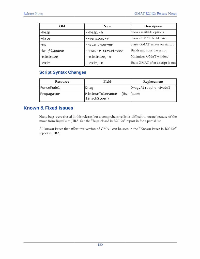
Release Notes GMAT R2012a Release Notes
180
Old New Description
-help --help, -h Shows available options
-date --version, -v Shows GMAT build date
-ms --start-server Starts GMAT server on startup
-br filename --run, -r scriptname Builds and runs the script
-minimize --minimize, -m Minimizes GMAT window
-exit --exit, -x Exits GMAT after a script is run
Script Syntax Changes
Resource Field Replacement
ForceModel Drag Drag.AtmosphereModel
Propagator MinimumTolerance (Bu-lirschStoer)
(none)
Known & Fixed Issues
Many bugs were closed in this release, but a comprehensive list is difficult to create because of themove from Bugzilla to JIRA. See the "Bugs closed in R2012a" report in for a partial list.
All known issues that affect this version of GMAT can be seen in the "Known issues in R2012a"report in JIRA.

Index
181
IndexAAchieve, 120Array, 51
BBaryCenter, 52BeginFiniteBurn, 121BeginMissionSequence, 122BodyNames, 52
CCallGmatFunction, 123CallMatlabFunction, 125ClearPlot, 126
EElse, 127EndFiniteBurn, 128EndFor, 130EndTarget, 152Equation, 129
FFor, 130
GGlobal, 133
IIf, 134
MManeuver, 136MarkPoint, 137Minimize, 138
NNonlinearConstraint, 139
OOptimize, 141
PPenDown, 143
PenUp, 142Propagate, 144
RReport, 147
SSave, 148SaveMission, 149ScriptEvent, 150Spacecraft, 97Stop, 151
TTarget, 152Toggle, 156
VVary, 157
WWhile, 160
Top Related