


Languages
Pages
Legal


Game Architecture2/6/15: Splines
Brought to you by Squirrel Eiserloh

Overview
» Averaging and Blending» Interpolation» Parametric Equations» Parametric Curves and Splines
including: Bézier splines (linear, quadratic, cubic) Cubic Hermite splines Catmull-Rom splines Cardinal splines Kochanek–Bartels splines B-splines
Demo 7,8,9

Averaging and Blending
Averaging and Blending
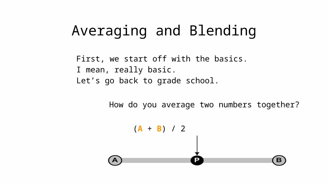
First, we start off with the basics.I mean, really basic.Let’s go back to grade school.
How do you average two numbers together?
(A + B) / 2

Averaging and Blending
Let’s change that around a bit.
(A + B) / 2
becomes
(.5 * A) + (.5 * B)
i.e. “half of A, half of B”, or“a 50/50 blend of A and B”
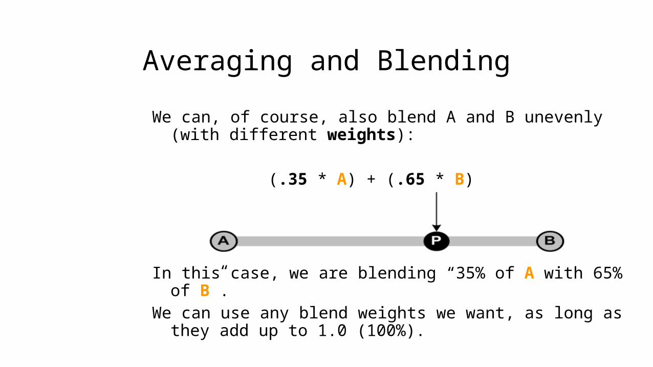
We can, of course, also blend A and B unevenly (with different weights):
(.35 * A) + (.65 * B)
In this case, we are blending “35% of A with 65% of B”.We can use any blend weights we want, as long as they add
up to 1.0 (100%).
Averaging and Blending
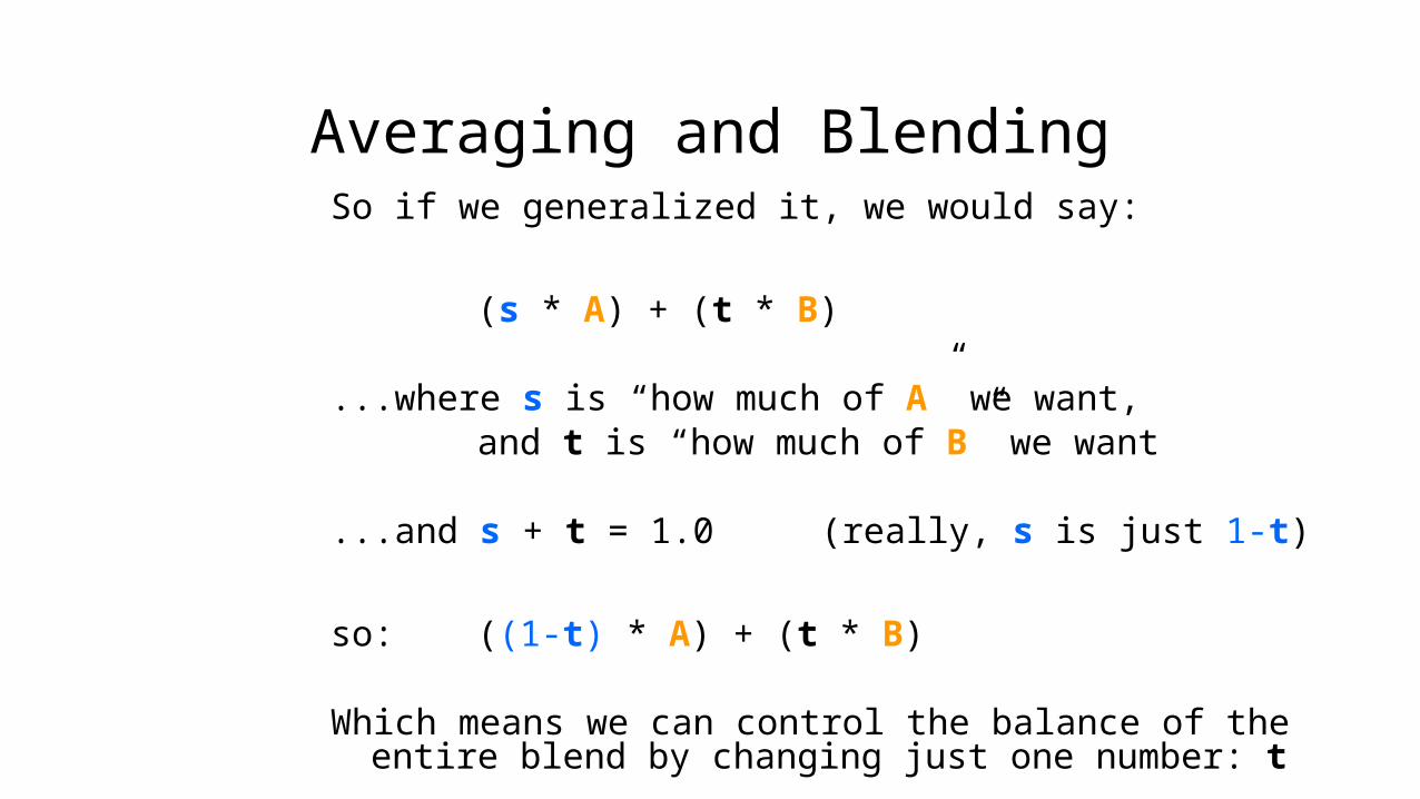
Averaging and BlendingSo if we generalized it, we would say:
(s * A) + (t * B)
...where s is “how much of A ” we want,and t is “how much of B” we want
...and s + t = 1.0 (really, s is just 1-t)
so: ((1-t) * A) + (t * B)
Which means we can control the balance of the entire blend by changing just one number: t
Averaging and Blending
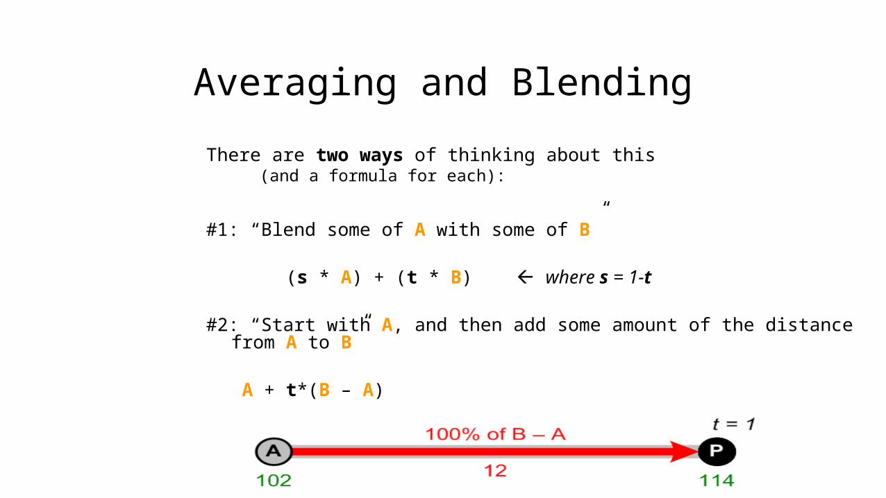
There are two ways of thinking about this (and a formula for each):
#1: “Blend some of A with some of B ”
(s * A) + (t * B) where s = 1-t
#2: “Start with A, and then add some amount of the distance from A to B ”
A + t*(B – A)
Averaging and Blending
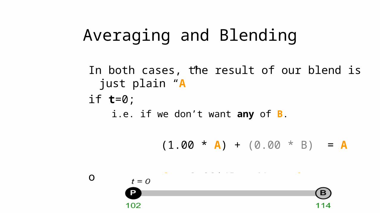
In both cases, the result of our blend is just plain “A”
if t=0; i.e. if we don’t want any of B.
(1.00 * A) + (0.00 * B) = A
or: A + 0.00*(B – A) = A
Averaging and Blending
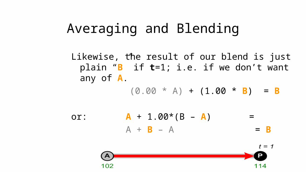
Likewise, the result of our blend is just plain “B” if t=1; i.e. if we don’t want any of A.
(0.00 * A) + (1.00 * B) = B
or: A + 1.00*(B – A) =A + B – A = B
Averaging and Blending
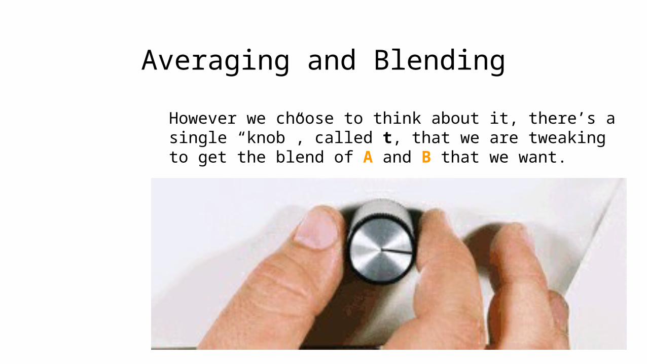
However we choose to think about it, there’s a single “knob”, called t, that we are tweaking to get the blend of A and B that we want.
Blending Compound Data
Blending Compound Data
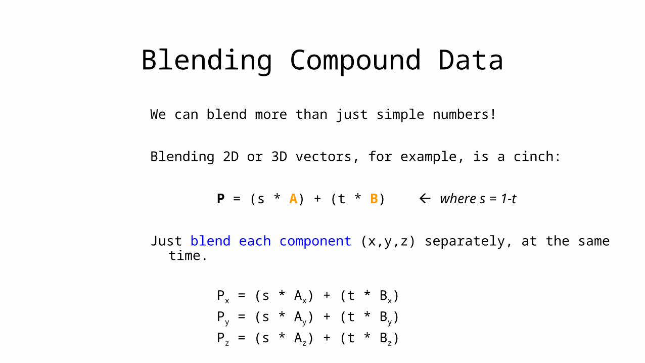
We can blend more than just simple numbers!
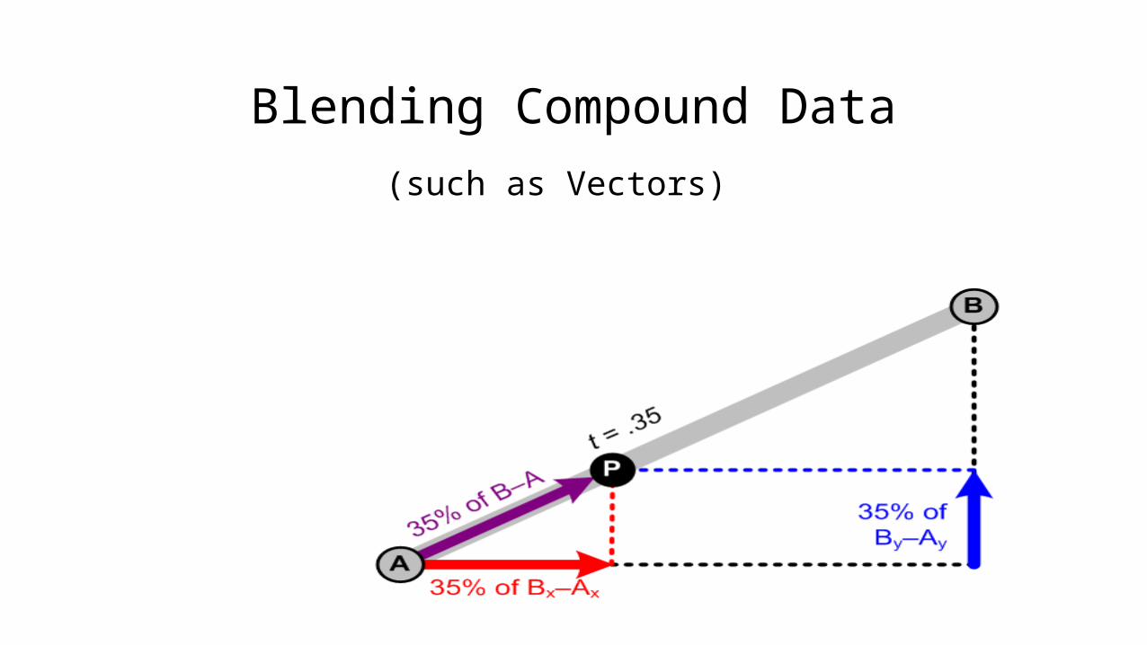
Blending 2D or 3D vectors, for example, is a cinch:
P = (s * A) + (t * B) where s = 1-t
Just blend each component (x,y,z) separately, at the same time.
Px = (s * Ax) + (t * Bx)
Py = (s * Ay) + (t * By)
Pz = (s * Az) + (t * Bz)
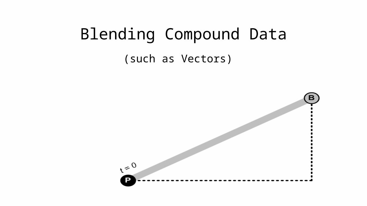
Blending Compound Data
(such as Vectors)
Blending Compound Data
(such as Vectors)

Blending Compound Data
(such as Vectors)

Blending Compound Data
(such as Vectors)
Blending Compound Data
Need to be careful, though!
Not all compound data types will blend correctly with this approach.
Examples: Color RGBs, Euler angles (yaw/pitch/roll), Matrices, Quaternions...
...in fact, there are a bunch that won’t.

Blending Compound Data
Here’s an RGB color example:
If A is RGB( 255, 0, 0 ) – bright red...and B is RGB( 0, 255, 0 ) – bright green
Blending the two (with t = 0.5) gives:RGB( 127, 127, 0 ) ...which is a dull, swampy color. Yuck.

Blending Compound Data
What we wanted was this:
...and what we got instead was this:

Blending Compound DataFor many compound classes, like RGB, you may need to write your own Blend() method that “does the right thing”, whatever that may be.
(For example, when interpolating RGBs you might consider converting to HSV, blending, then converting back to RGB at the end.)
Will talk later about what happens when you try to blend Euler Angles (yaw/pitch/roll), Matrices, and Quaternions using this simple “naïve” approach of blending the components.
Interpolation

Interpolation
Interpolation (also called “Lerping”) is just changing blend weights to do blending over time.i.e. Turning the knob (t) progressively, not just setting it to some position.Often we crank slowly from t=0 to t=1.
Interpolation
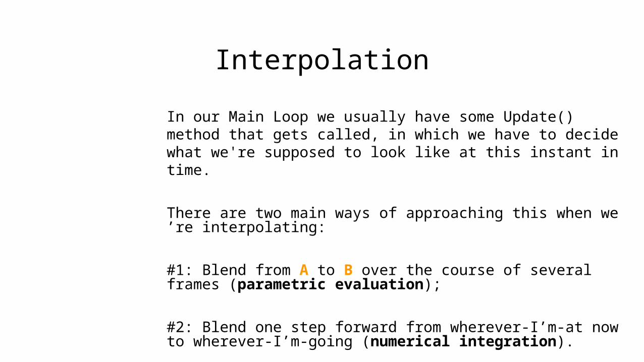
In our Main Loop we usually have some Update() method that gets called, in which we have to decide what we're supposed to look like at this instant in time.
There are two main ways of approaching this when we’re interpolating:
#1: Blend from A to B over the course of several frames (parametric evaluation);
#2: Blend one step forward from wherever-I’m-at now to wherever-I’m-going (numerical integration).
Interpolation
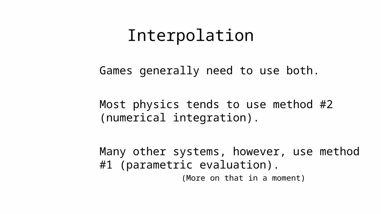
Games generally need to use both.
Most physics tends to use method #2 (numerical integration).
Many other systems, however, use method #1 (parametric evaluation).
(More on that in a moment)

Interpolation
We use “lerping”all the time, under
different names.
For example:
an Audio crossfade

Interpolation
We use “lerping”all the time, under
different names.
For example:
an Audio crossfade
or this simple
PowerPoint effect.

Interpolation
Basically:
whenever we do any sort of blend over time
we’re lerping (interpolating)
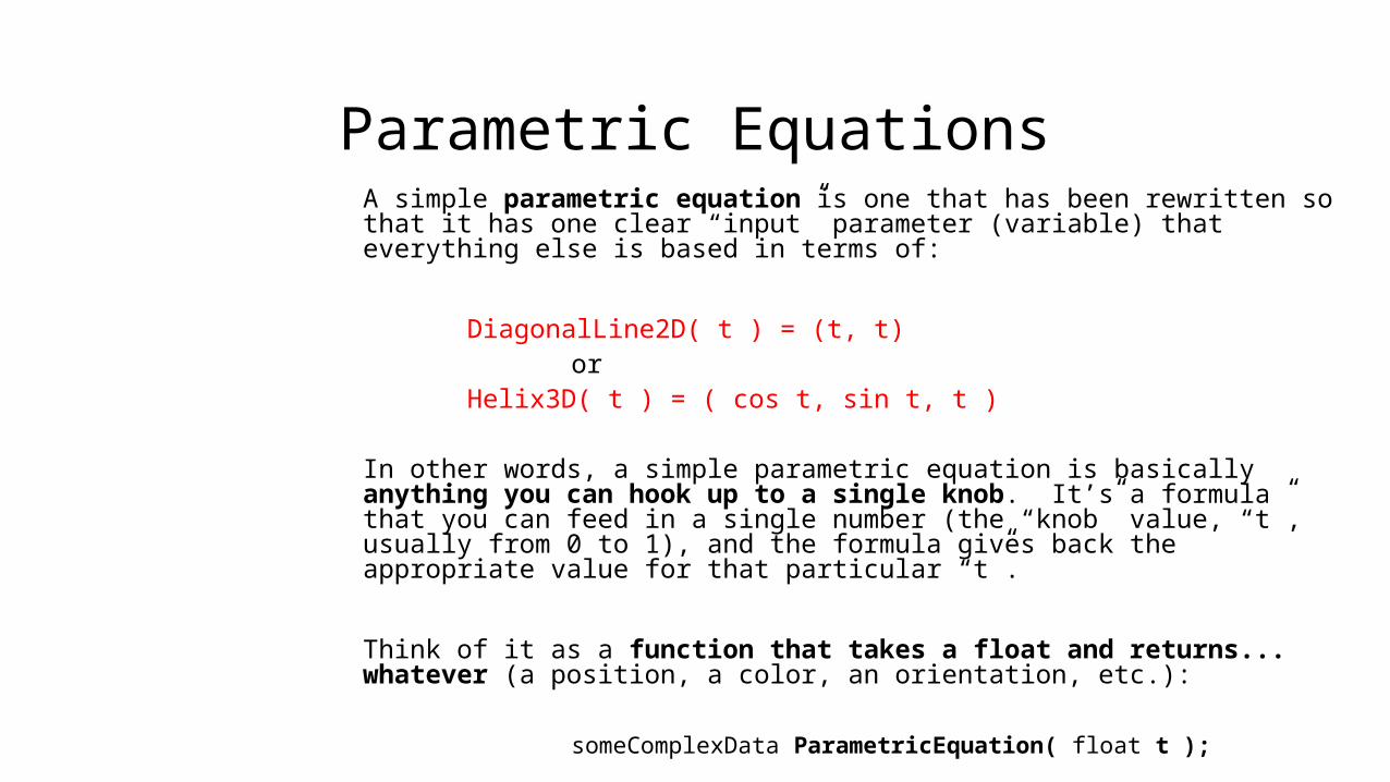
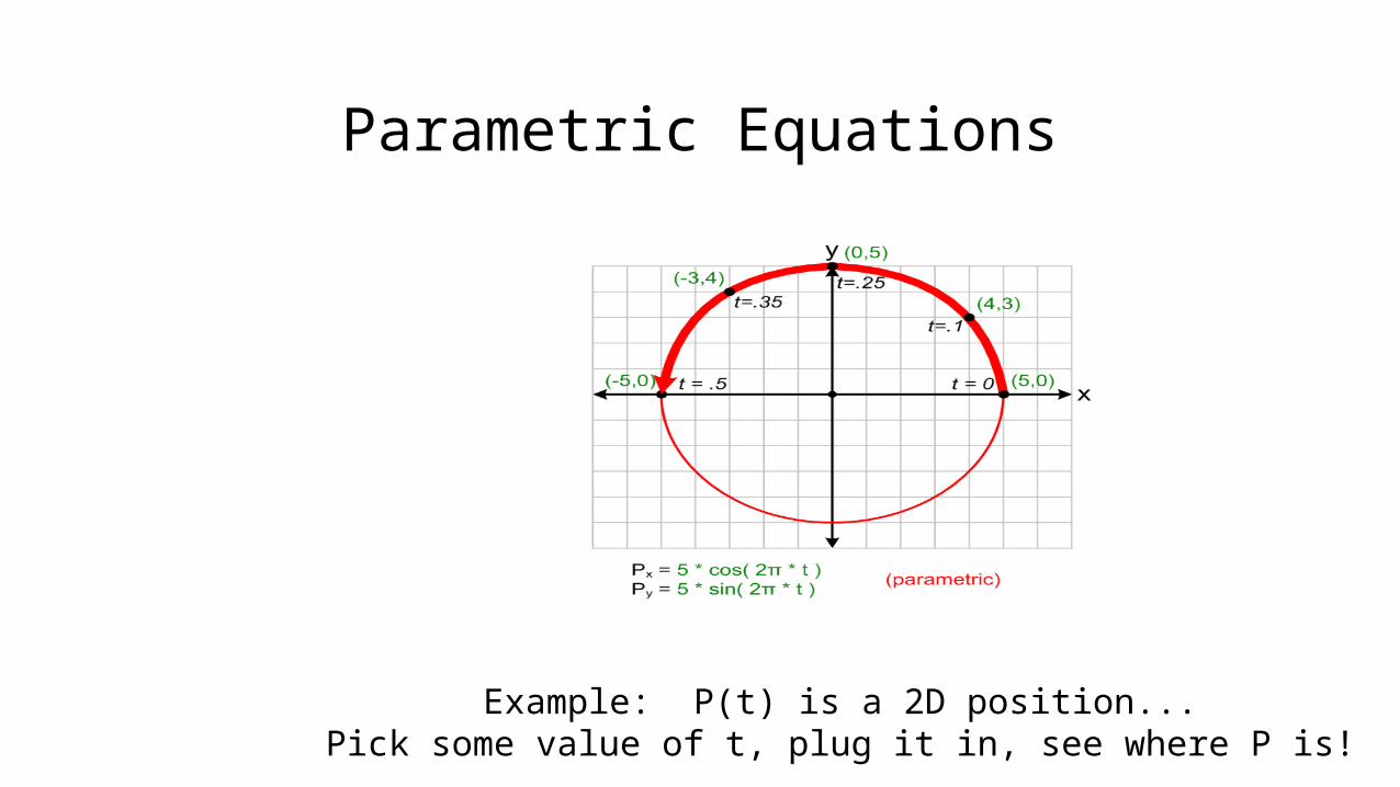
Parametric EquationsA simple parametric equation is one that has been rewritten so that it has one clear “input” parameter (variable) that everything else is based in terms of:
DiagonalLine2D( t ) = (t, t)or
Helix3D( t ) = ( cos t, sin t, t )
In other words, a simple parametric equation is basically anything you can hook up to a single knob. It’s a formula that you can feed in a single number (the “knob” value, “t”, usually from 0 to 1), and the formula gives back the appropriate value for that particular “t”.
Think of it as a function that takes a float and returns... whatever (a position, a color, an orientation, etc.):
someComplexData ParametricEquation( float t );

Parametric Equations
Essentially:
P(t) = some formula with “t” in it
...as t changes, P changes(P depends upon t)
P(t) can return any kind of value; whatever we want to interpolate, for instance.
Position (2D, 3D, etc.) Orientation Scale Alpha etc.

Parametric Equations
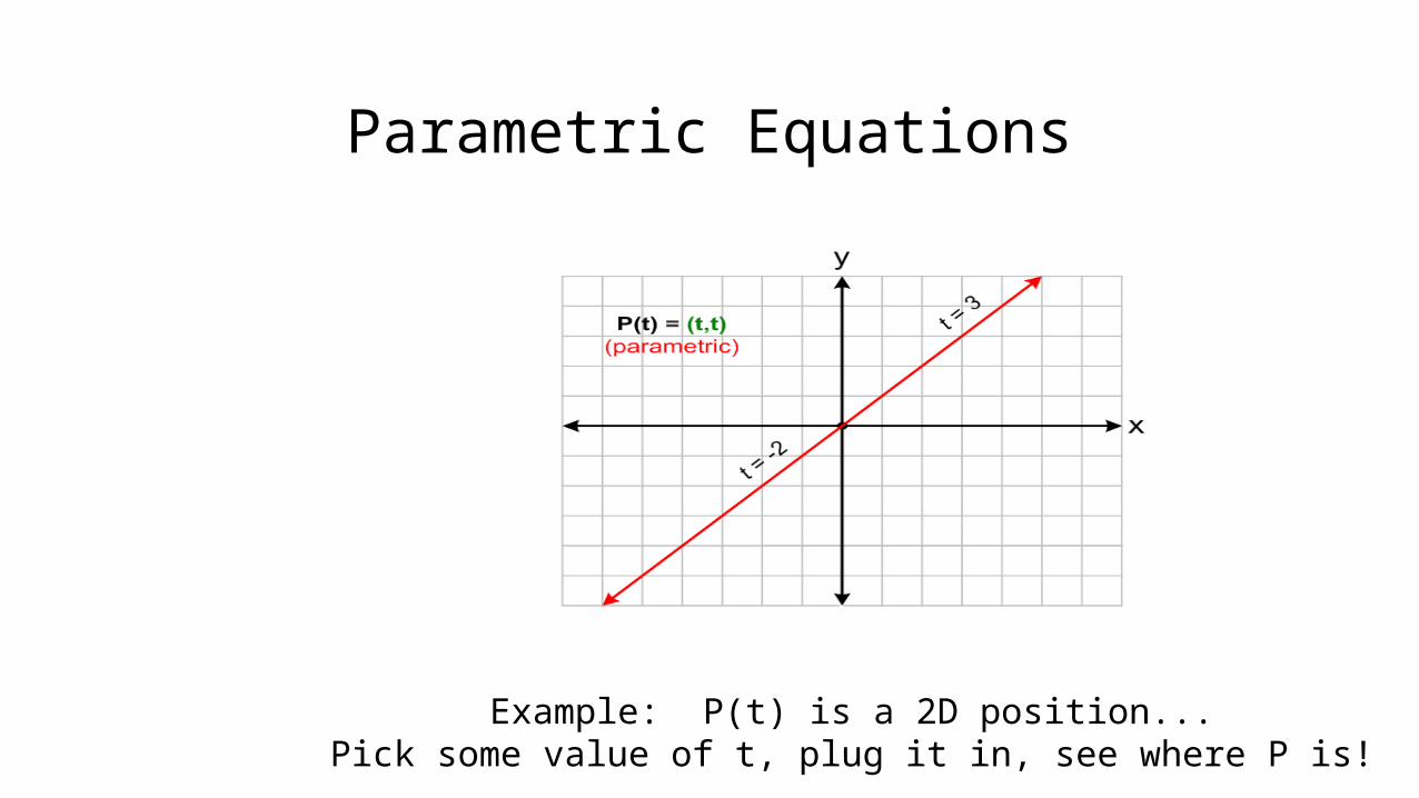
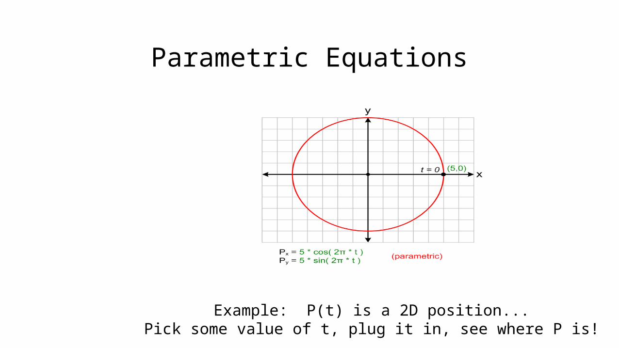
Example: P(t) is a 2D position...Pick some value of t, plug it in, see where P is!
Parametric Equations
Example: P(t) is a 2D position...Pick some value of t, plug it in, see where P is!

Parametric Equations
Example: P(t) is a 2D position...Pick some value of t, plug it in, see where P is!
Parametric Equations
Example: P(t) is a 2D position...Pick some value of t, plug it in, see where P is!

Parametric Equations
Example: P(t) is a 2D position...Pick some value of t, plug it in, see where P is!

Parametric Equations
Example: P(t) is a 2D position...Pick some value of t, plug it in, see where P is!
Parametric Equations
Example: P(t) is a 2D position...Pick some value of t, plug it in, see where P is!

Parametric Equations
Example: P(t) is a 2D position...Pick some value of t, plug it in, see where P is!
Parametric Curves
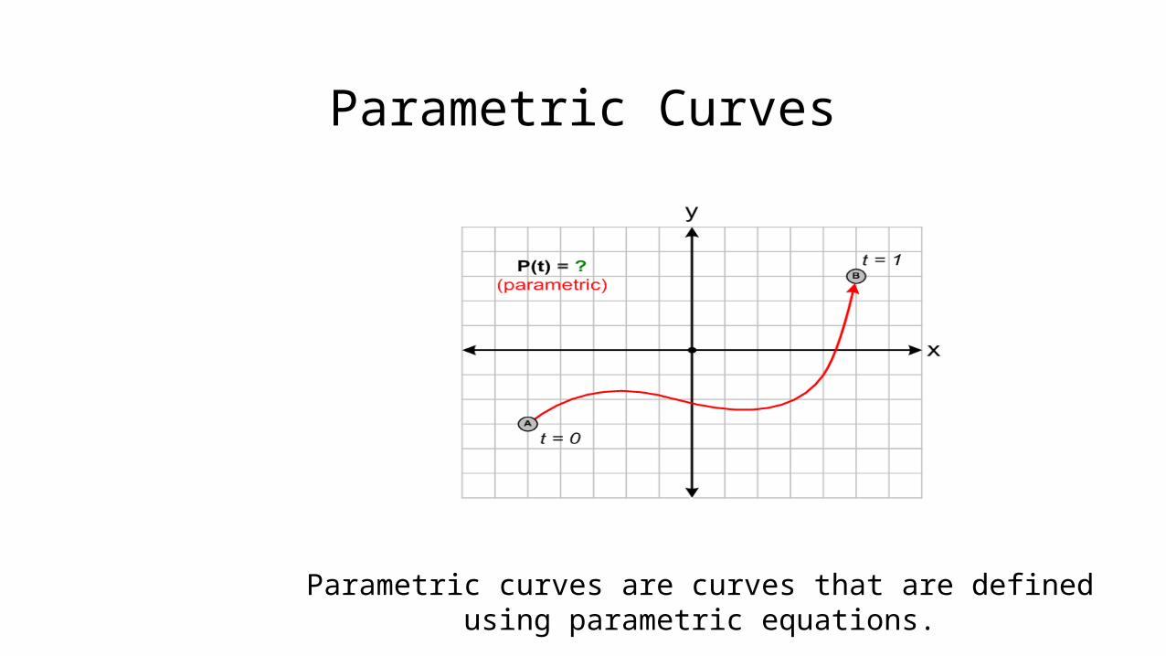
Parametric Curves
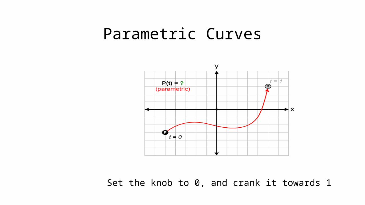
Parametric curves are curves that are definedusing parametric equations.
Parametric Curves
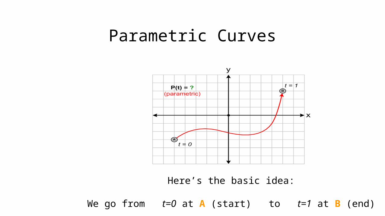
Here’s the basic idea:
We go from t=0 at A (start) to t=1 at B (end)
Parametric Curves
Set the knob to 0, and crank it towards 1
Parametric Curves
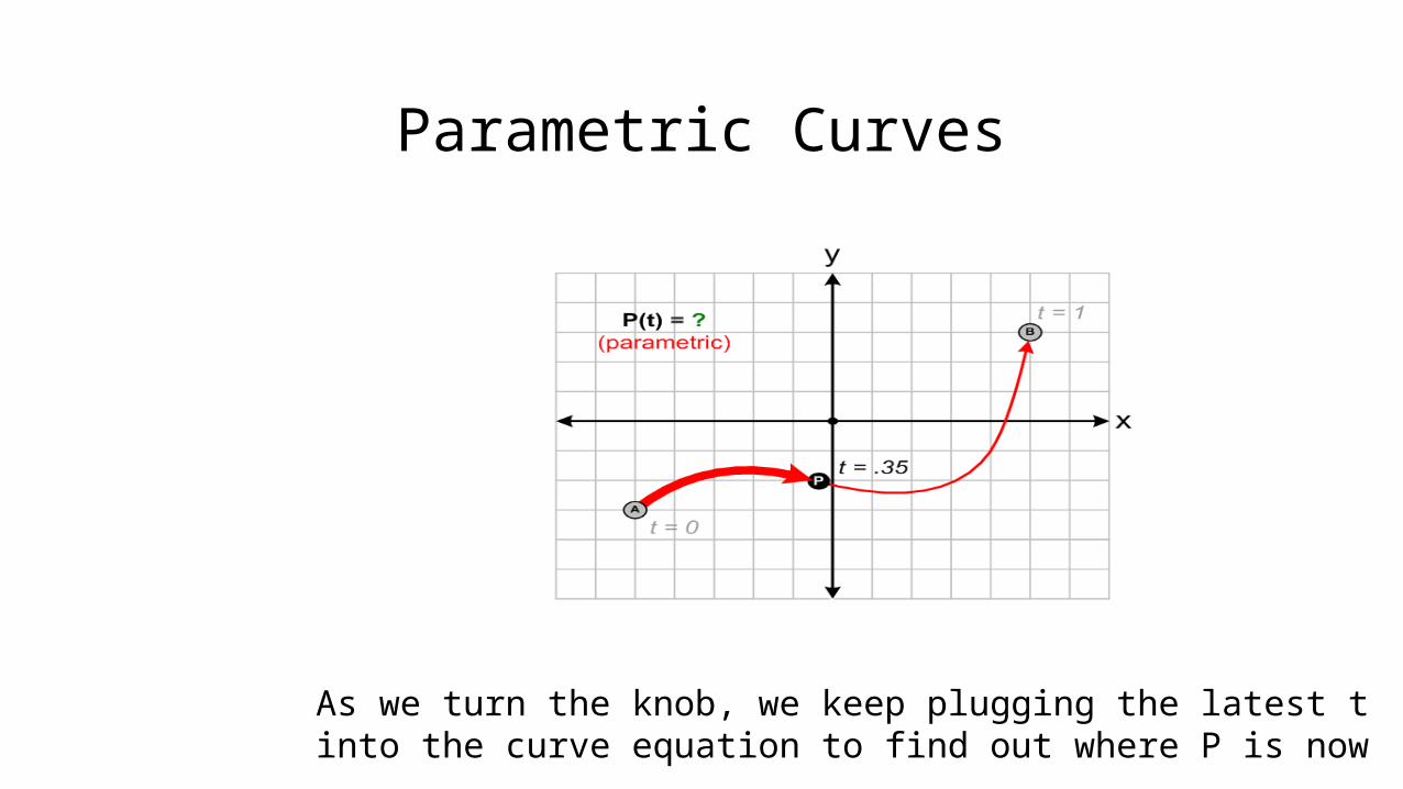
As we turn the knob, we keep plugging the latest t into the curve equation to find out where P is now
Parametric Curves
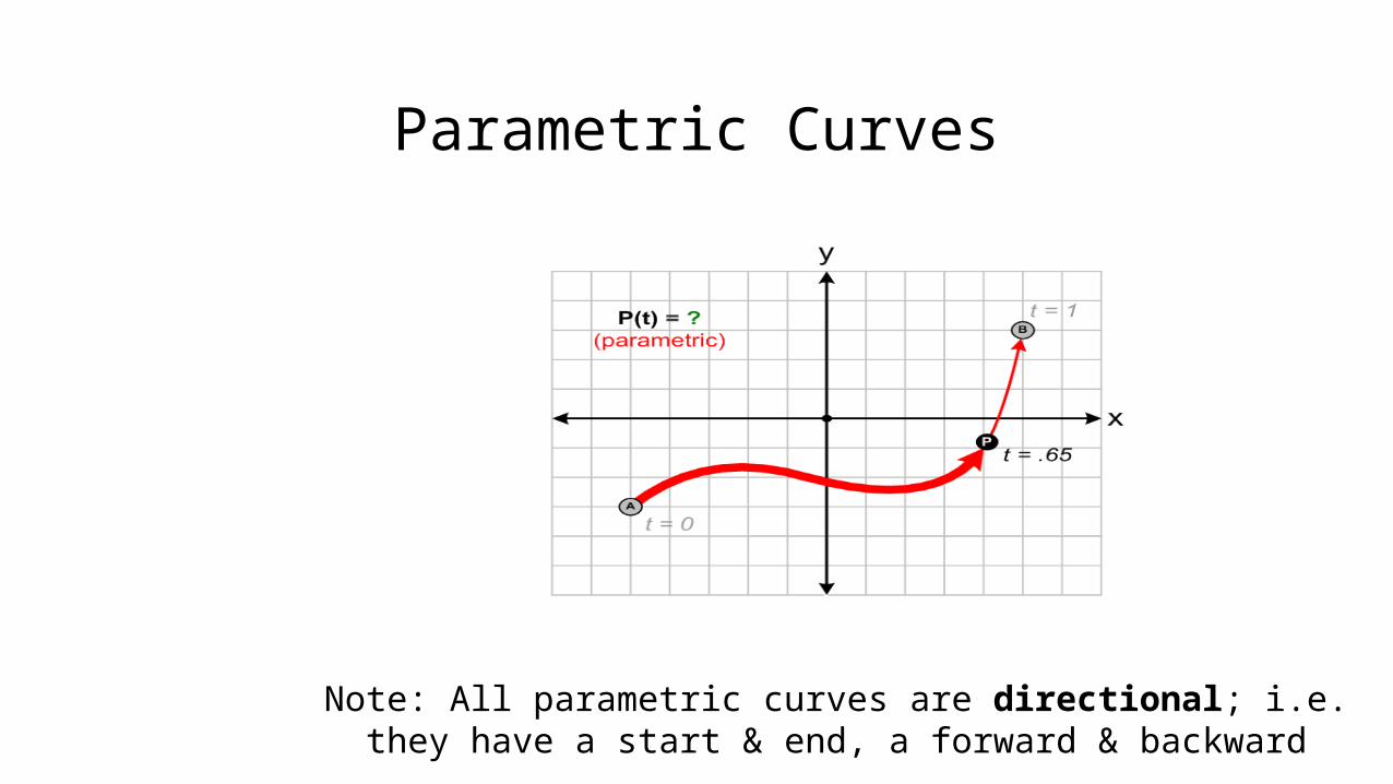
Note: All parametric curves are directional; i.e.they have a start & end, a forward & backward

Parametric Curves
So that’s the basic idea.
Now how do we actually do it?
Bézier Curves
(pronounced “bay-zeeyay”)

Linear Bézier Curves
Bezier curves are the easiest kind to understand.
The simplest kind of Bezier curves areLinear Bezier curves.
They’re so simple, they’re not even curvy!
Demo 1+P
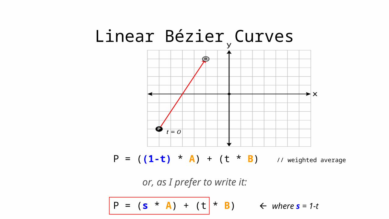
Linear Bézier Curves
P = ((1-t) * A) + (t * B) // weighted average
or, as I prefer to write it:
P = (s * A) + (t * B) where s = 1-t
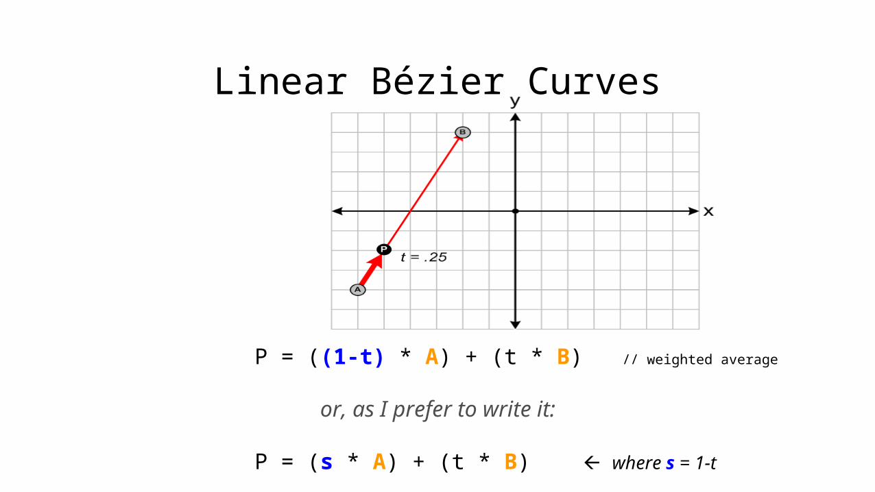
Linear Bézier Curves
P = ((1-t) * A) + (t * B) // weighted average
or, as I prefer to write it:
P = (s * A) + (t * B) where s = 1-t

Linear Bézier Curves
P = ((1-t) * A) + (t * B) // weighted average
or, as I prefer to write it:
P = (s * A) + (t * B) where s = 1-t
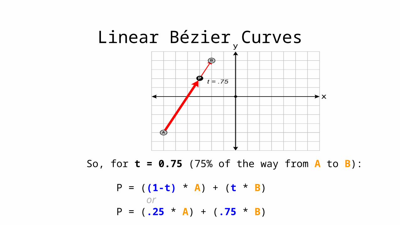
Linear Bézier Curves
So, for t = 0.75 (75% of the way from A to B):
P = ((1-t) * A) + (t * B)or
P = (.25 * A) + (.75 * B)
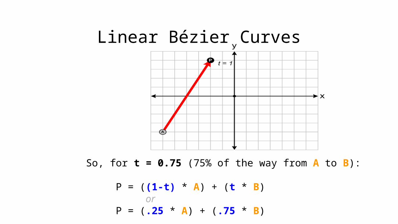
Linear Bézier Curves
So, for t = 0.75 (75% of the way from A to B):
P = ((1-t) * A) + (t * B)or
P = (.25 * A) + (.75 * B)
Quadratic Bézier Curves
Demo 4 (P)
Quadratic Bézier Curves
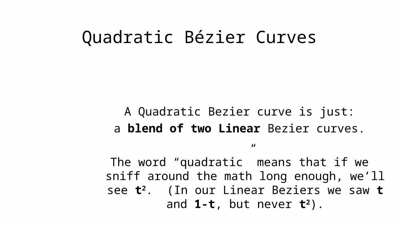
A Quadratic Bezier curve is just:a blend of two Linear Bezier curves.
The word “quadratic” means that if we sniff around the math long enough, we’ll see t2. (In our Linear Beziers we saw t and 1-t, but never
t2).
Quadratic Bézier Curves
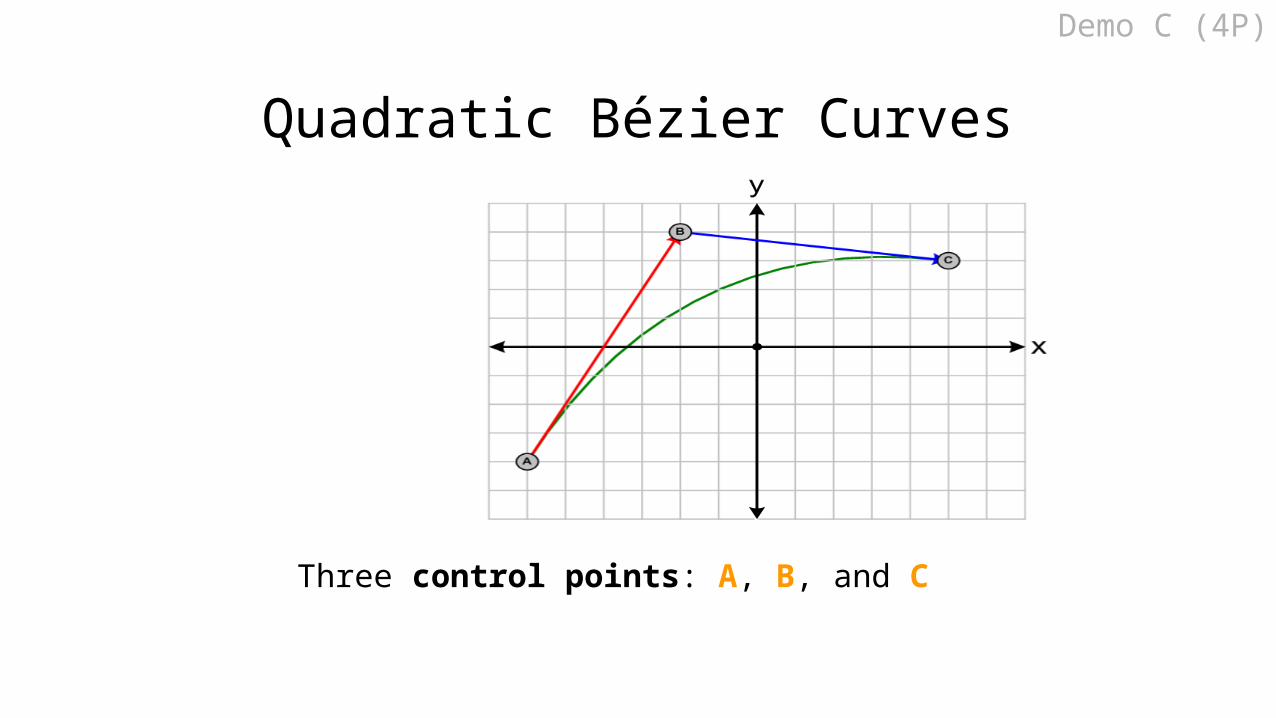
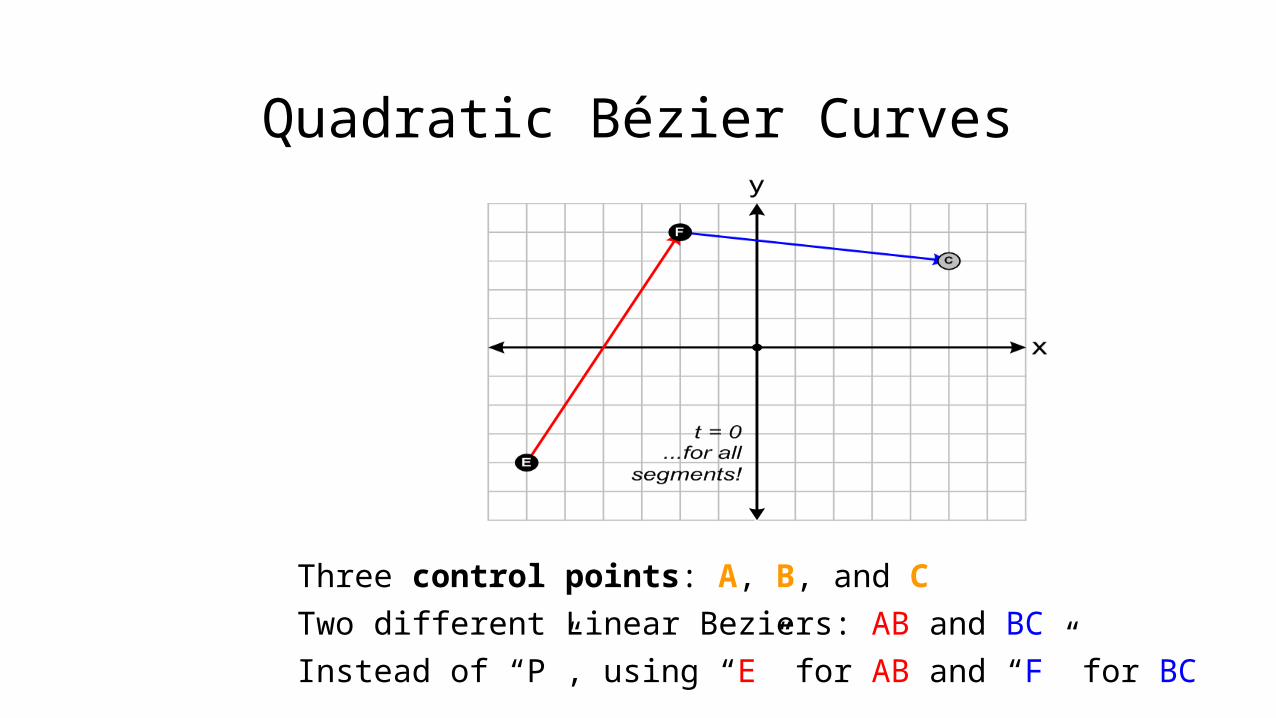
Three control points: A, B, and C
Demo C (4P)
Quadratic Bézier Curves
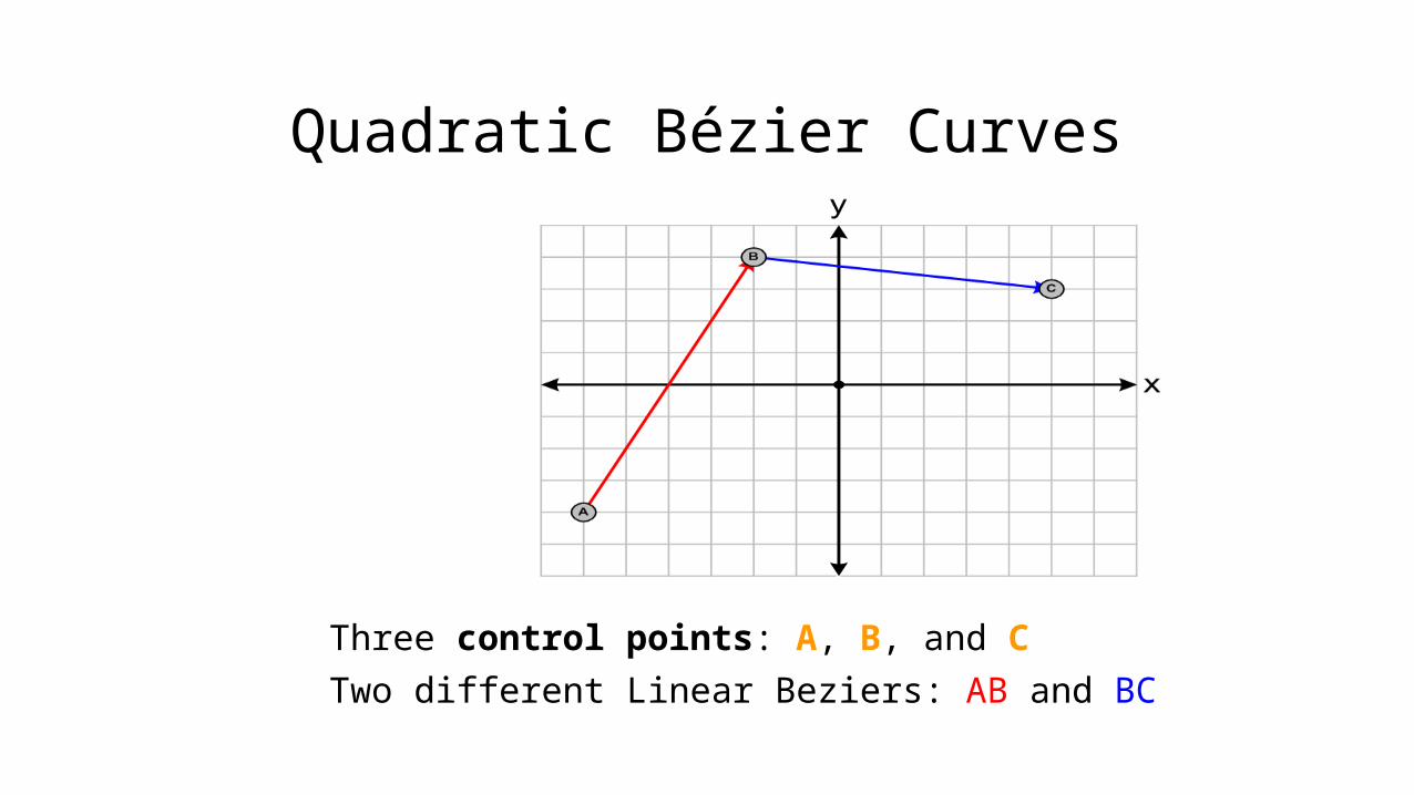
Three control points: A, B, and C
Two different Linear Beziers: AB and BC
Quadratic Bézier Curves
Three control points: A, B, and C
Two different Linear Beziers: AB and BC
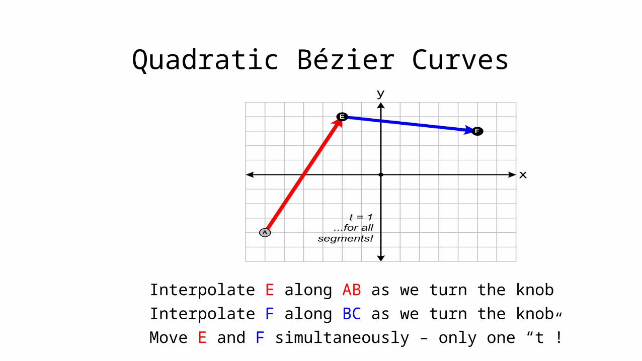
Instead of “P”, using “E” for AB and “F” for BC
Quadratic Bézier Curves
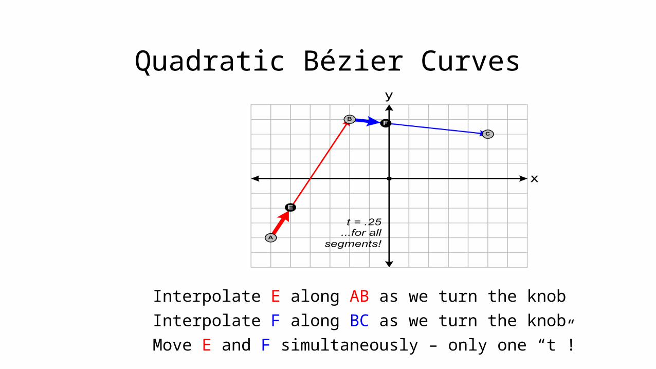
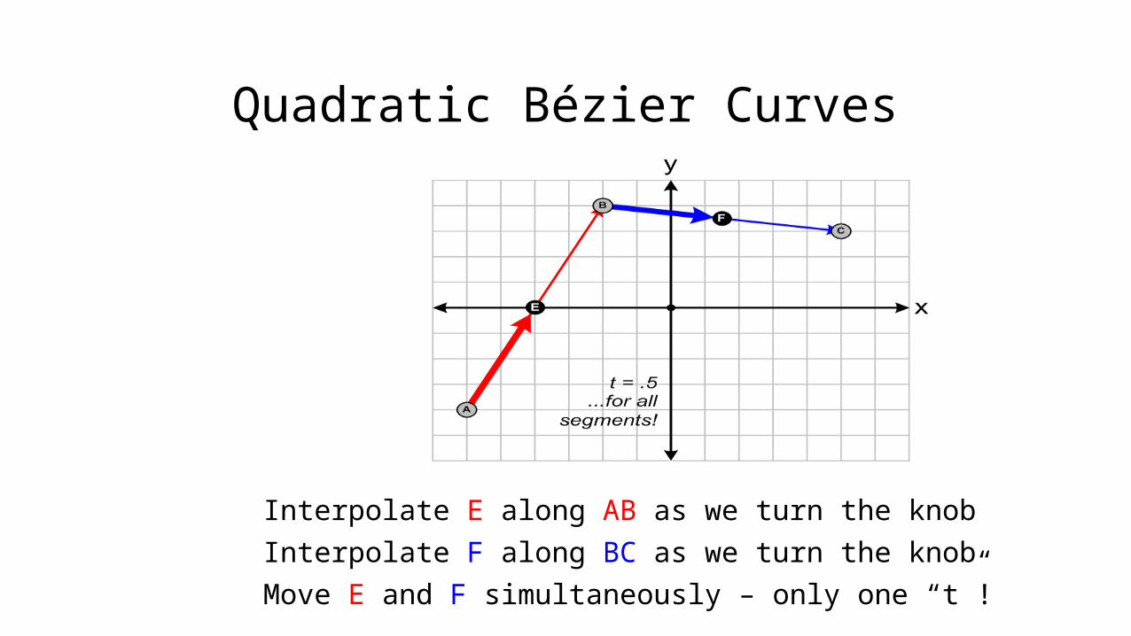
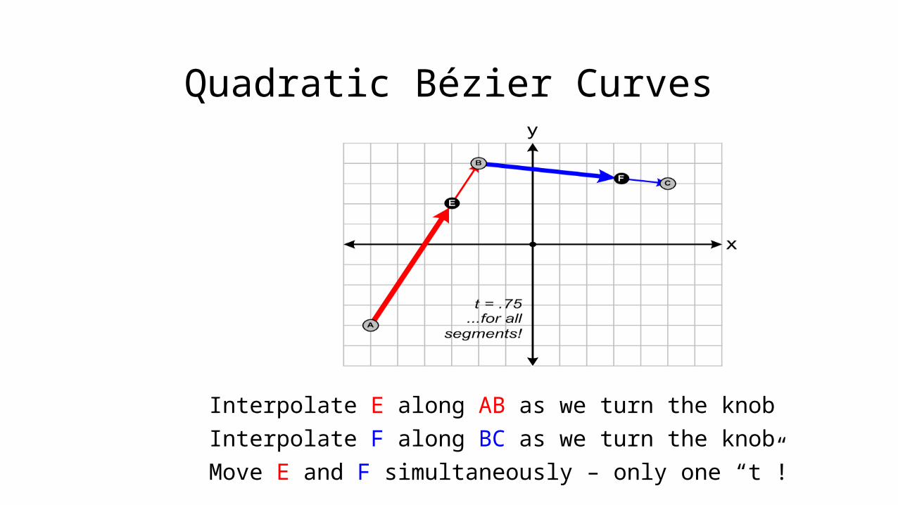
Interpolate E along AB as we turn the knob
Interpolate F along BC as we turn the knob
Move E and F simultaneously – only one “t”!
Quadratic Bézier Curves
Interpolate E along AB as we turn the knob
Interpolate F along BC as we turn the knob
Move E and F simultaneously – only one “t”!
Quadratic Bézier Curves
Interpolate E along AB as we turn the knob
Interpolate F along BC as we turn the knob
Move E and F simultaneously – only one “t”!
Quadratic Bézier Curves
Interpolate E along AB as we turn the knob
Interpolate F along BC as we turn the knob
Move E and F simultaneously – only one “t”!
Quadratic Bézier Curves
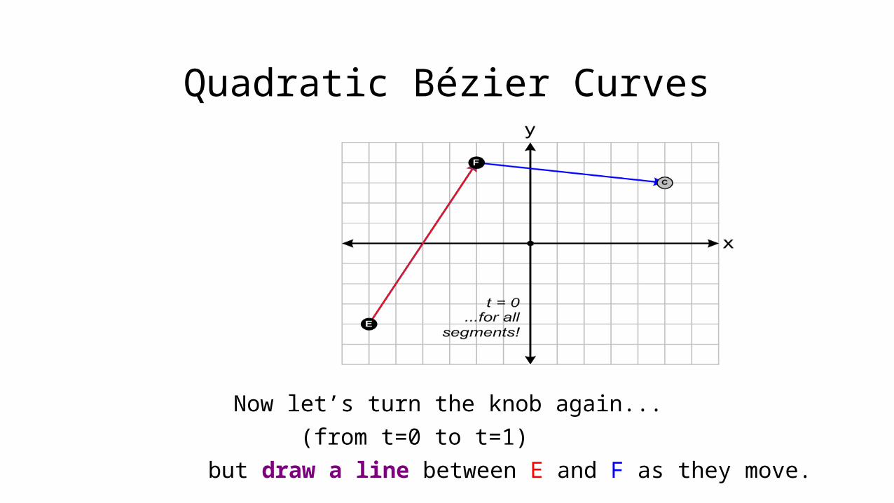
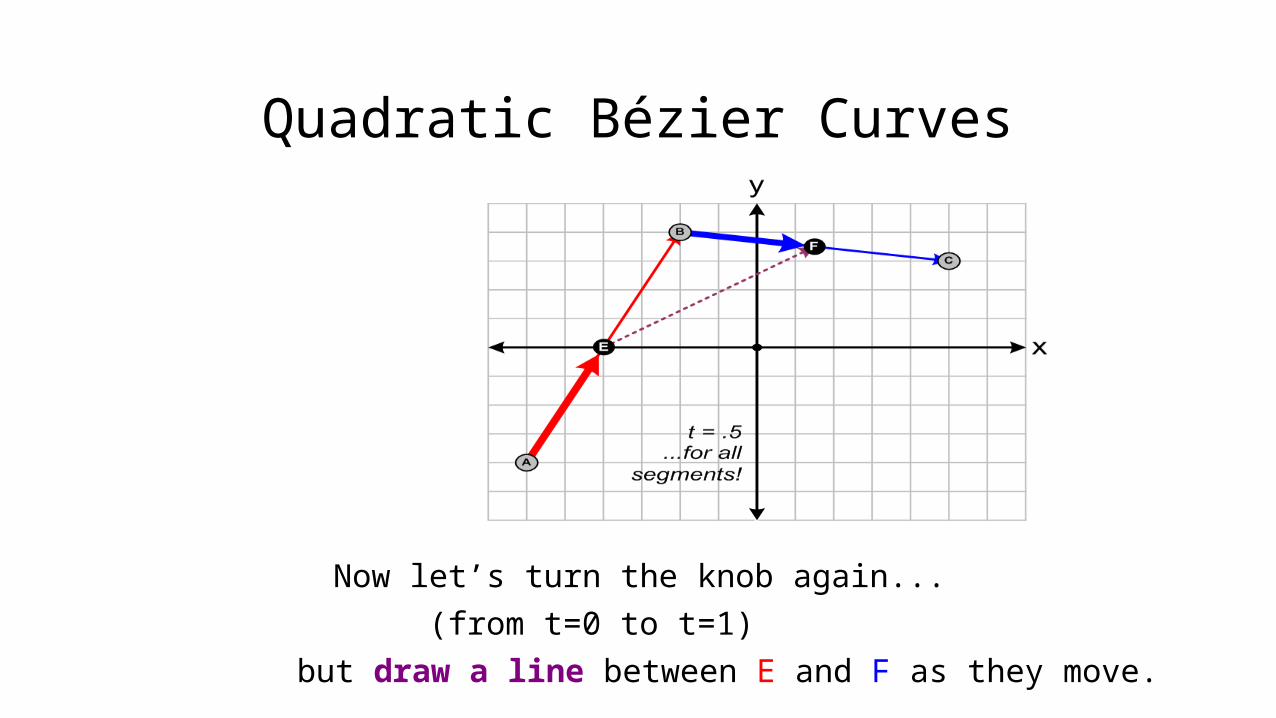
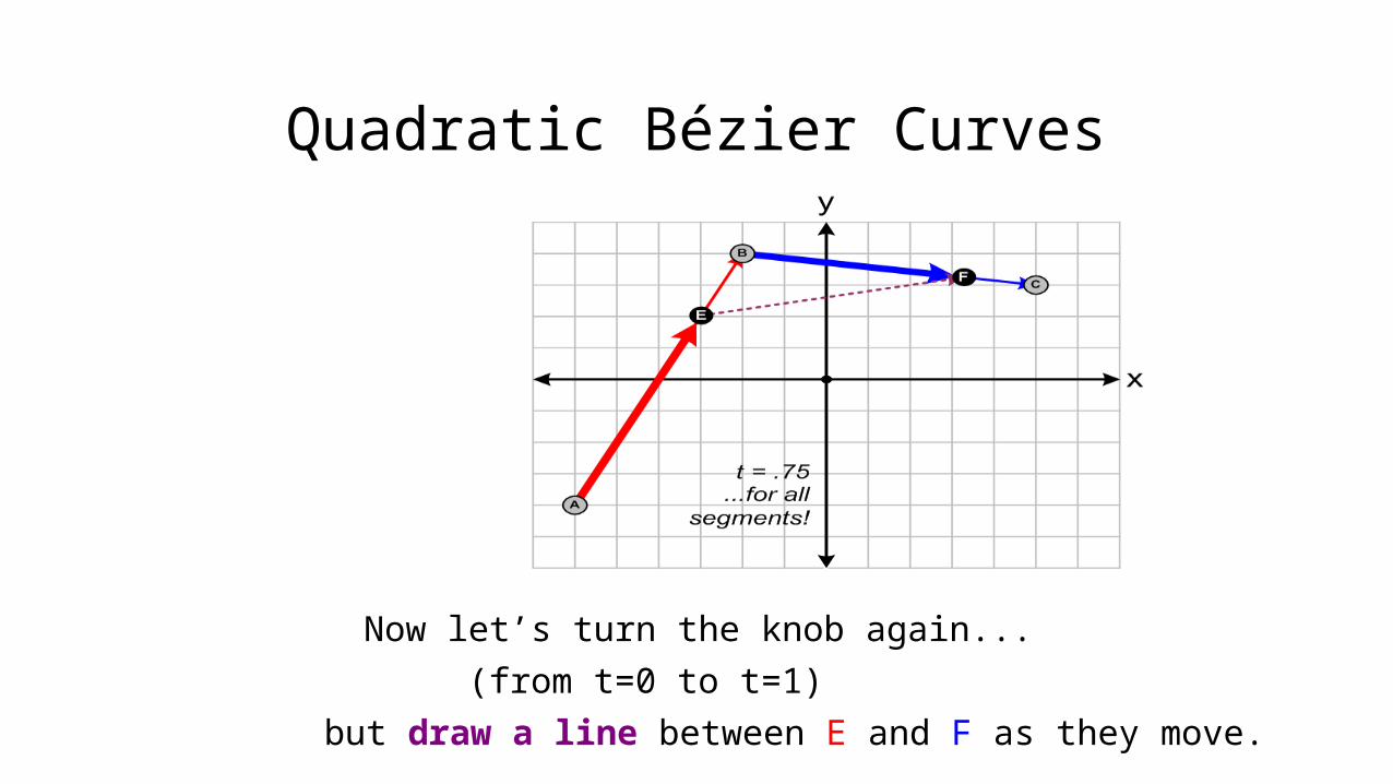
Now let’s turn the knob again...
(from t=0 to t=1)
but draw a line between E and F as they move.

Quadratic Bézier Curves
Now let’s turn the knob again...
(from t=0 to t=1)
but draw a line between E and F as they move.
Quadratic Bézier Curves
Now let’s turn the knob again...
(from t=0 to t=1)
but draw a line between E and F as they move.
Quadratic Bézier Curves
Now let’s turn the knob again...
(from t=0 to t=1)
but draw a line between E and F as they move.

Quadratic Bézier Curves
Now let’s turn the knob again...
(from t=0 to t=1)
but draw a line between E and F as they move.
Quadratic Bézier Curves
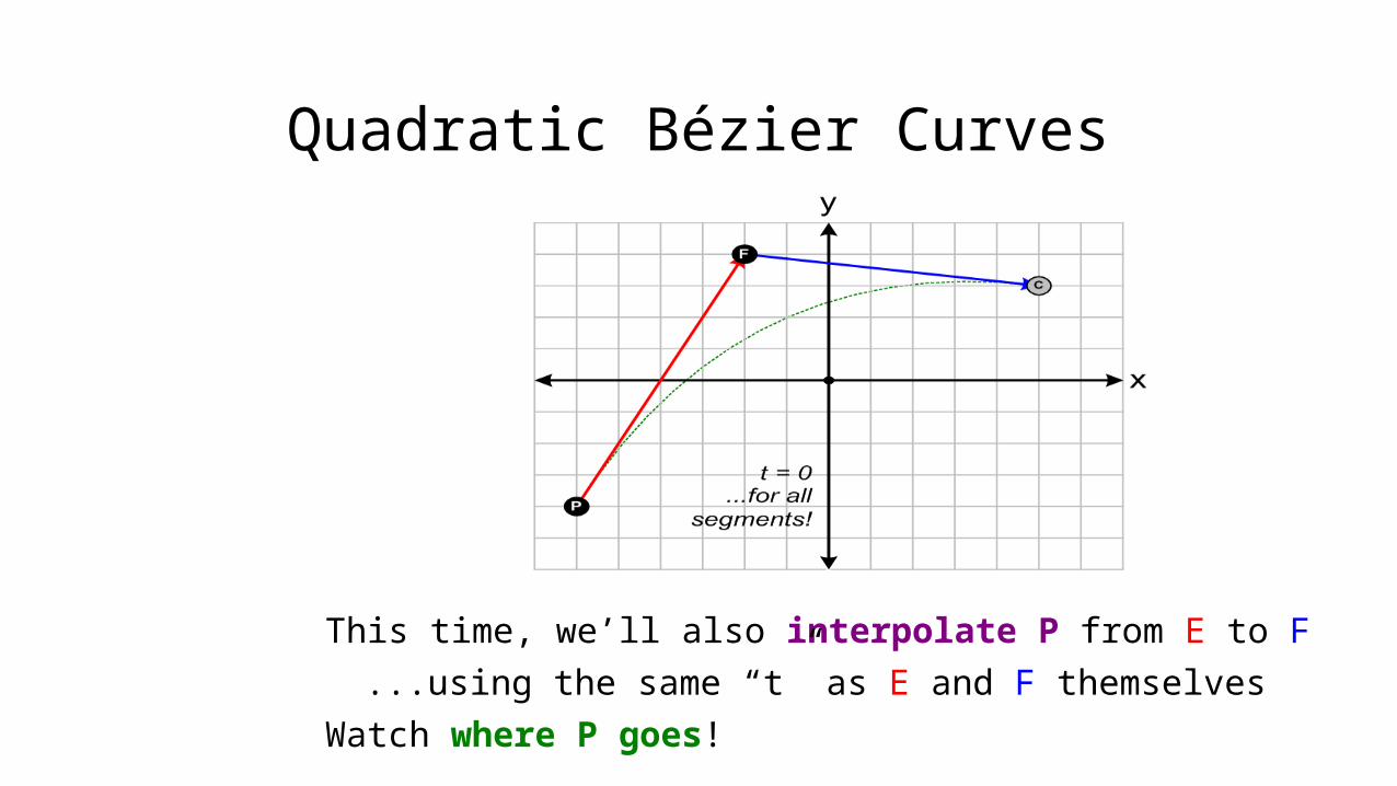
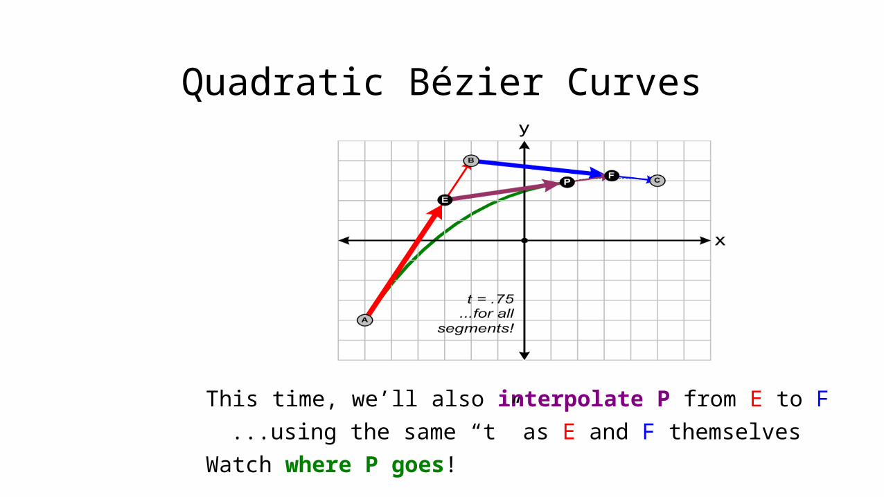
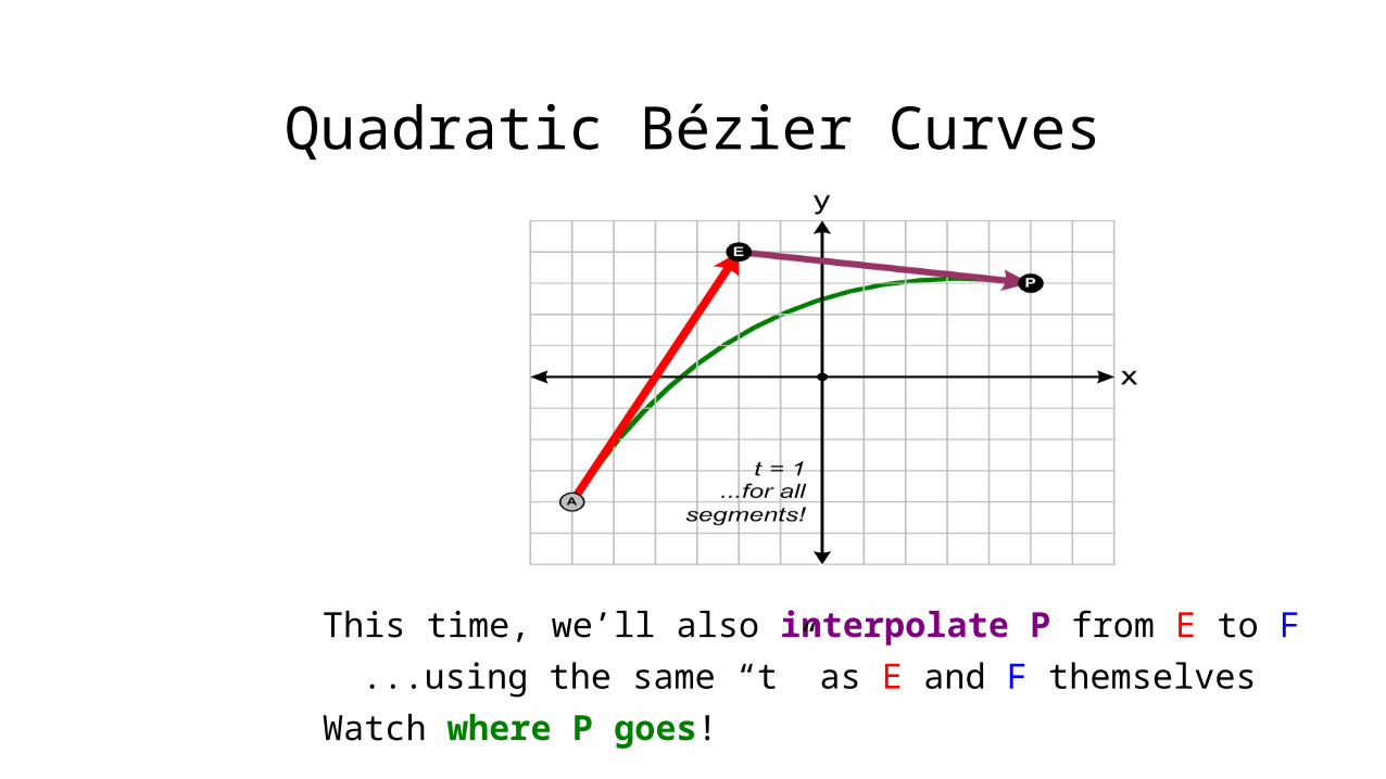
This time, we’ll also interpolate P from E to F
...using the same “t” as E and F themselves
Watch where P goes!

Quadratic Bézier Curves
This time, we’ll also interpolate P from E to F
...using the same “t” as E and F themselves
Watch where P goes!

Quadratic Bézier Curves
This time, we’ll also interpolate P from E to F
...using the same “t” as E and F themselves
Watch where P goes!
Quadratic Bézier Curves
This time, we’ll also interpolate P from E to F
...using the same “t” as E and F themselves
Watch where P goes!
Quadratic Bézier Curves
This time, we’ll also interpolate P from E to F
...using the same “t” as E and F themselves
Watch where P goes!

Quadratic Bézier Curves
Note that mathematicians use
P0, P1, P2 instead of A, B, C
I will keep using A, B, C here for simplicity and cleanliness
A
B
C
Quadratic Bézier Curves
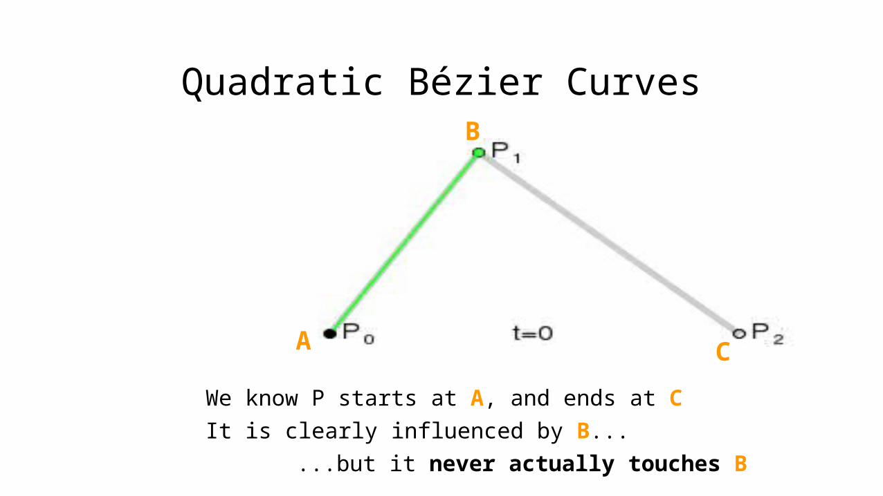
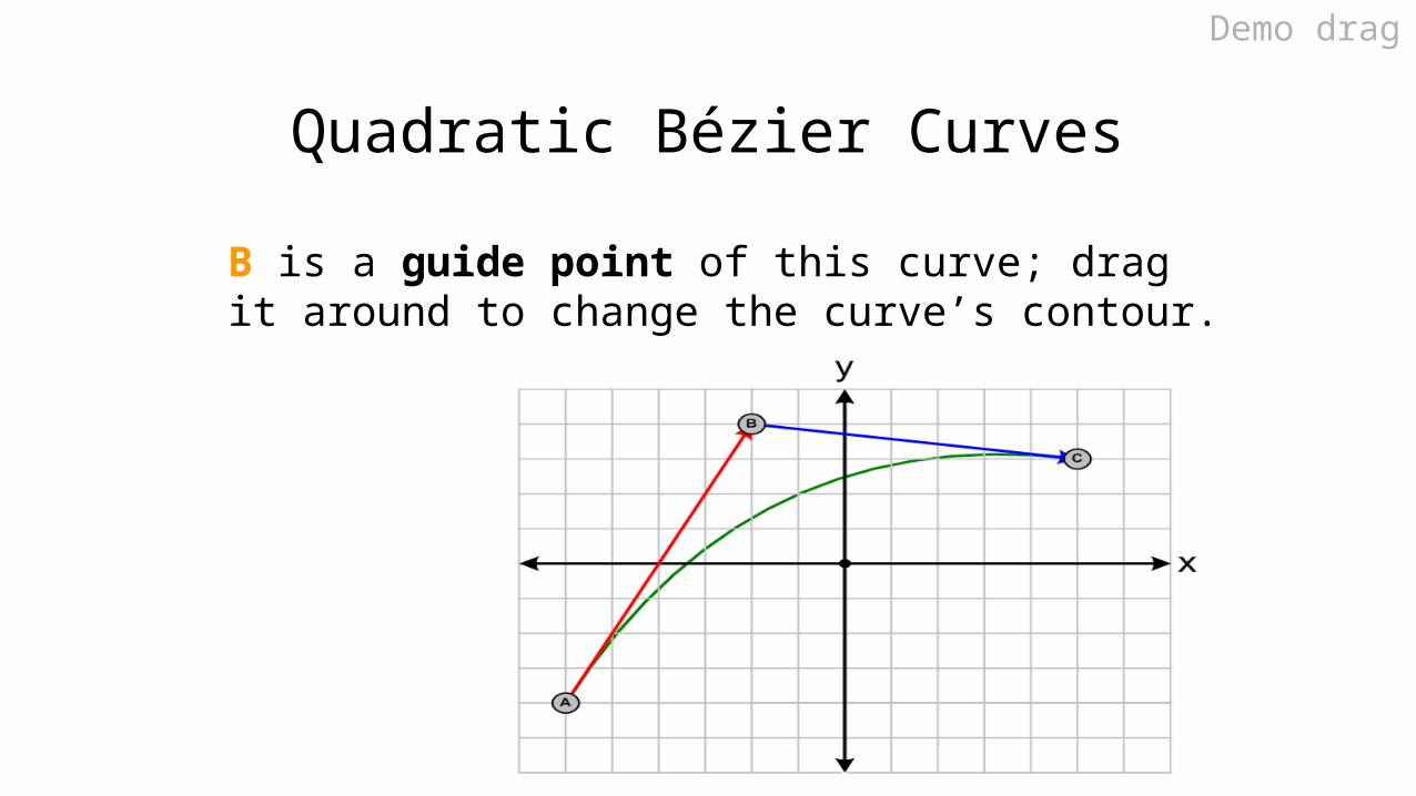
We know P starts at A, and ends at C
It is clearly influenced by B...
...but it never actually touches B
A
B
C
Quadratic Bézier Curves
B is a guide point of this curve; drag it around to change the curve’s contour.
Demo drag
Quadratic Bézier Curves
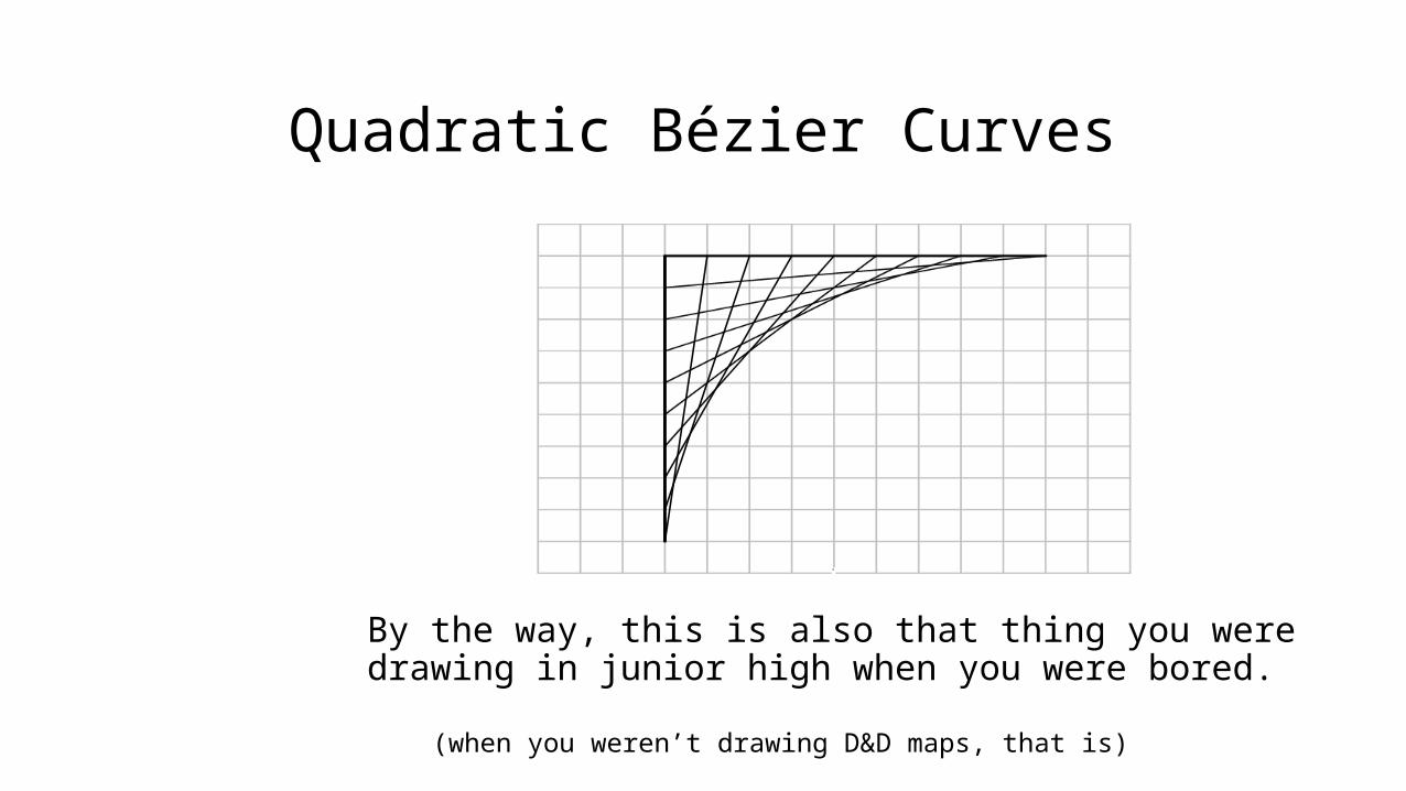
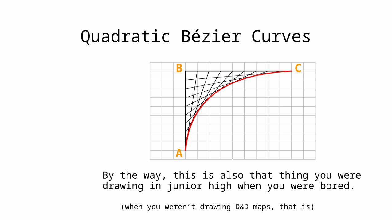
By the way, this is also that thing you were drawing in junior high when you were bored.
(when you weren’t drawing D&D maps, that is)
Quadratic Bézier Curves
By the way, this is also that thing you were drawing in junior high when you were bored.
(when you weren’t drawing D&D maps, that is)
A
B C
Quadratic Bézier Curves
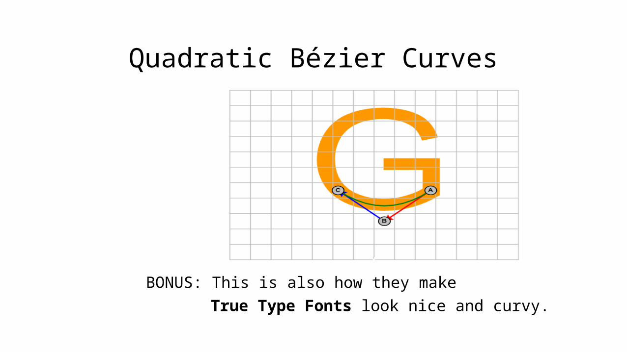
BONUS: This is also how they make
True Type Fonts look nice and curvy.
Quadratic Bézier Curves
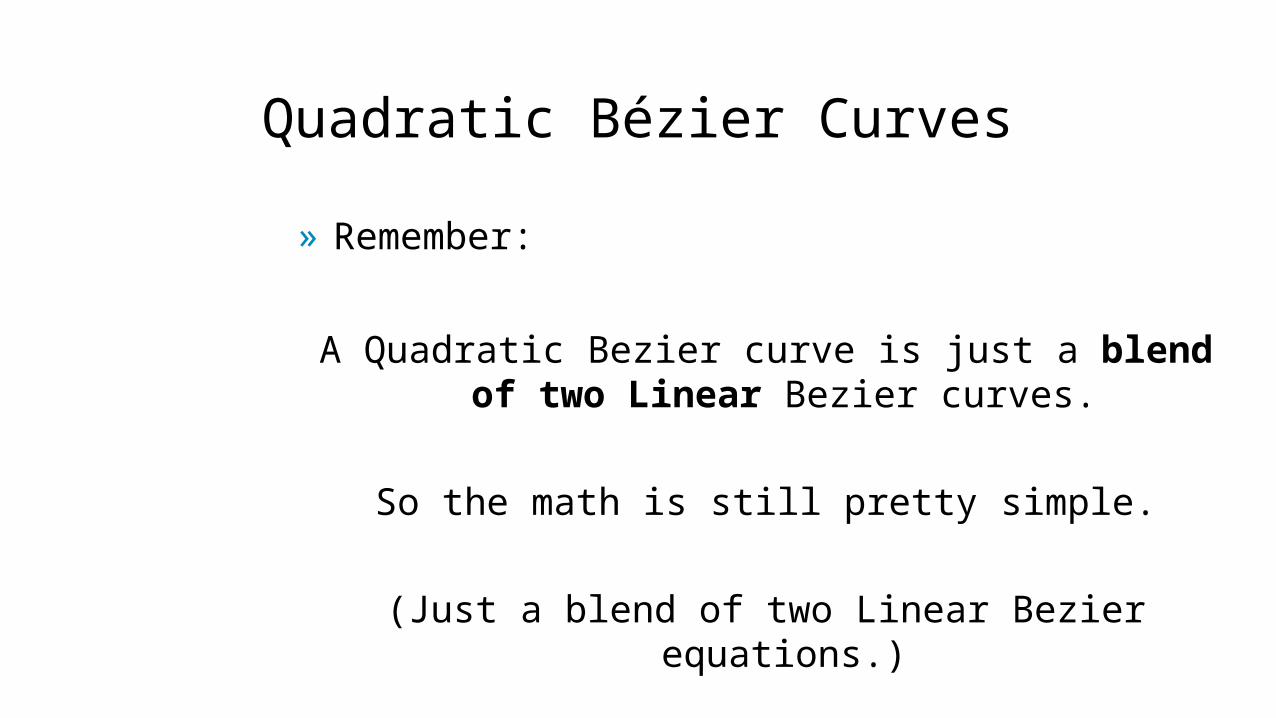
» Remember:
A Quadratic Bezier curve is just a blend of two Linear Bezier curves.
So the math is still pretty simple.
(Just a blend of two Linear Bezier equations.)

Quadratic Bézier Curves
E(t) = (s * A) + (t * B) where s = 1-t
F(t) = (s * B) + (t * C)
P(t) = (s * E) + (t * F) technically E(t) and F(t) here

Quadratic Bézier Curves
» Hold on! You said “quadratic” meant we’d see a t2 in there somewhere.
E(t) = sA + tB
F(t) = sB + tC
P(t) = sE(t) + tF(t)
» P(t) is an interpolation from E(t) to F(t)» When you plug the E(t) and F(t) equations into the P(t)
equation, you get...
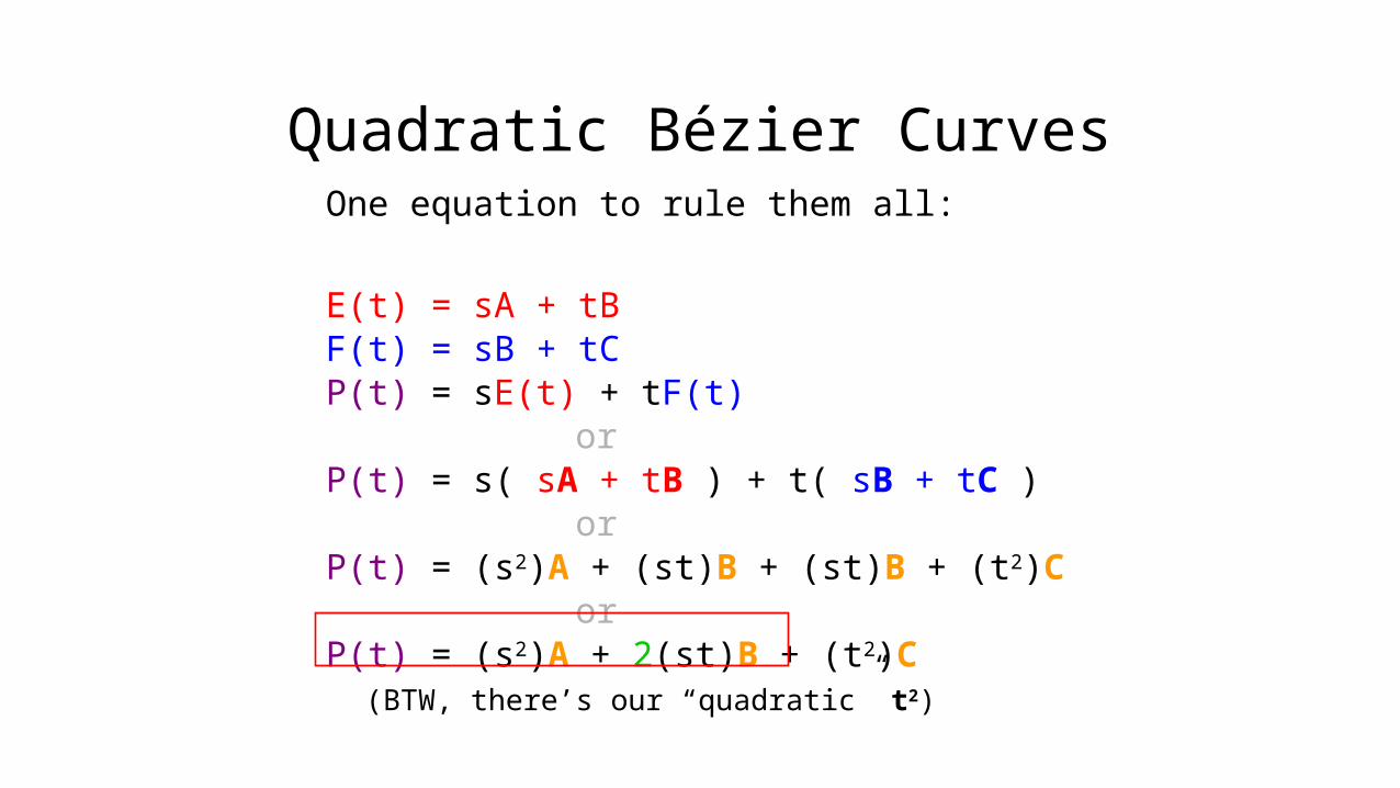
Quadratic Bézier CurvesOne equation to rule them all:
E(t) = sA + tBF(t) = sB + tCP(t) = sE(t) + tF(t)
orP(t) = s( sA + tB ) + t( sB + tC )
orP(t) = (s2)A + (st)B + (st)B + (t2)C
orP(t) = (s2)A + 2(st)B + (t2)C
(BTW, there’s our “quadratic” t2)
Quadratic Bézier Curves
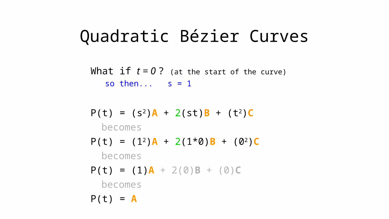
What if t = 0 ? (at the start of the curve)
so then... s = 1
P(t) = (s2)A + 2(st)B + (t2)C
becomes
P(t) = (12)A + 2(1*0)B + (02)C
becomes
P(t) = (1)A + 2(0)B + (0)C
becomes
P(t) = A
Quadratic Bézier Curves
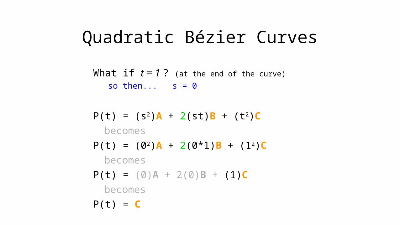
What if t = 1 ? (at the end of the curve)
so then... s = 0
P(t) = (s2)A + 2(st)B + (t2)C
becomes
P(t) = (02)A + 2(0*1)B + (12)C
becomes
P(t) = (0)A + 2(0)B + (1)C
becomes
P(t) = C

Non-uniformityBe careful: most curves are not uniform; that is, they have variable “density” or “speed” throughout them. (However, we can also use this to our advantage!)
Demo drag

Cubic Bézier Curves
Demo 4PC -> 5

Cubic Bézier Curves
A Cubic Bezier curve is just:a blend of two Quadratic Bezier curves.
The word “cubic” means that if we sniff around the math long enough, we’ll see t3. (In our
Linear Beziers we saw t; in our Quadratics we saw t2).
T-30
Cubic Bézier Curves
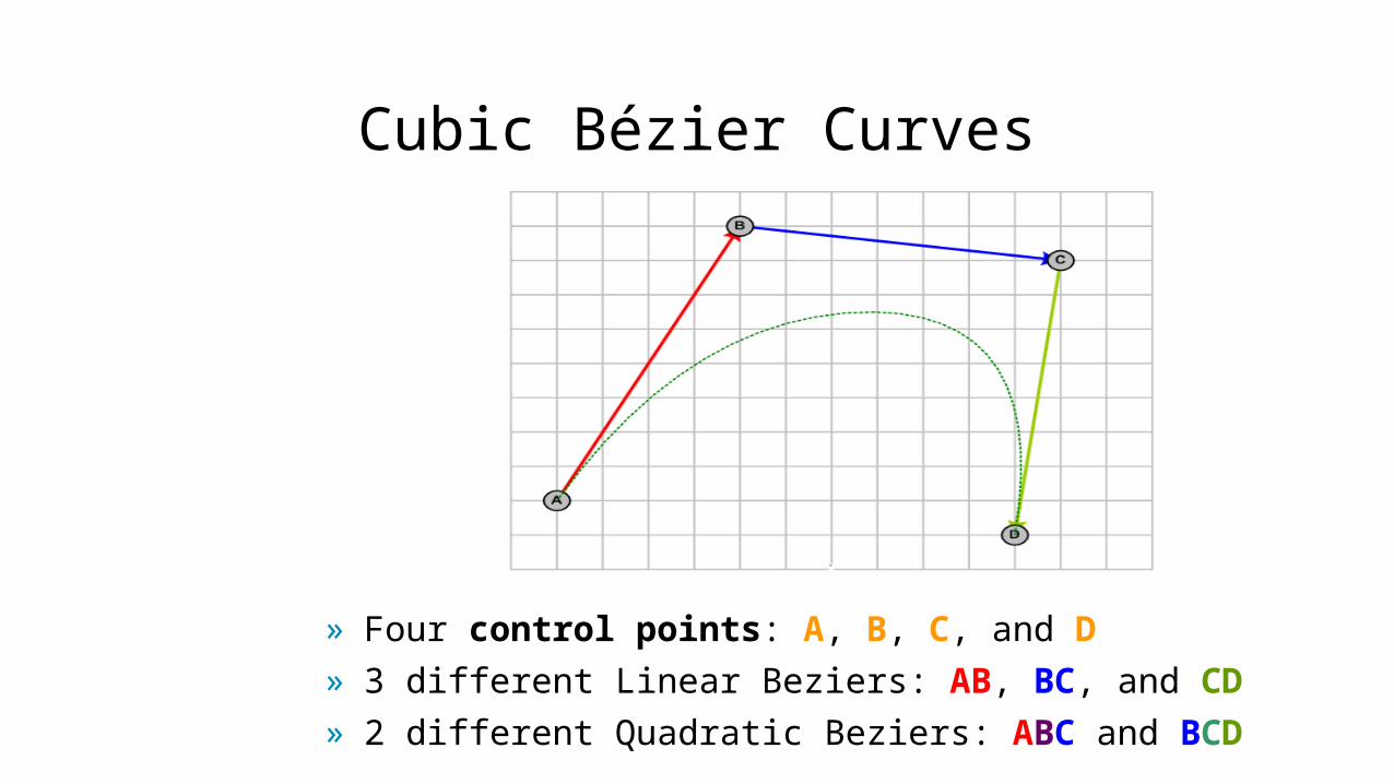
» Four control points: A, B, C, and D» 3 different Linear Beziers: AB, BC, and CD» 2 different Quadratic Beziers: ABC and BCD
Cubic Bézier Curves
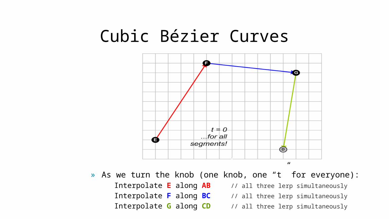
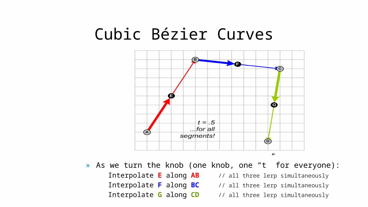
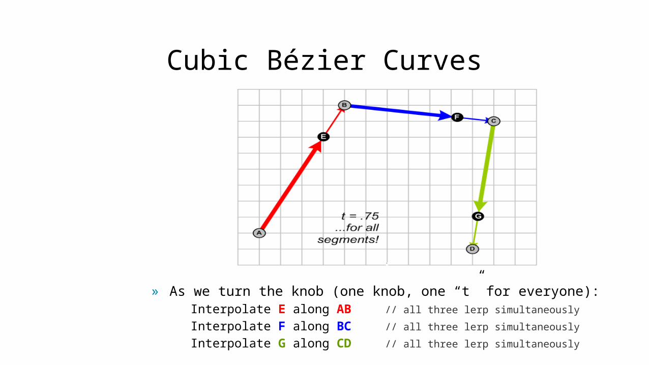
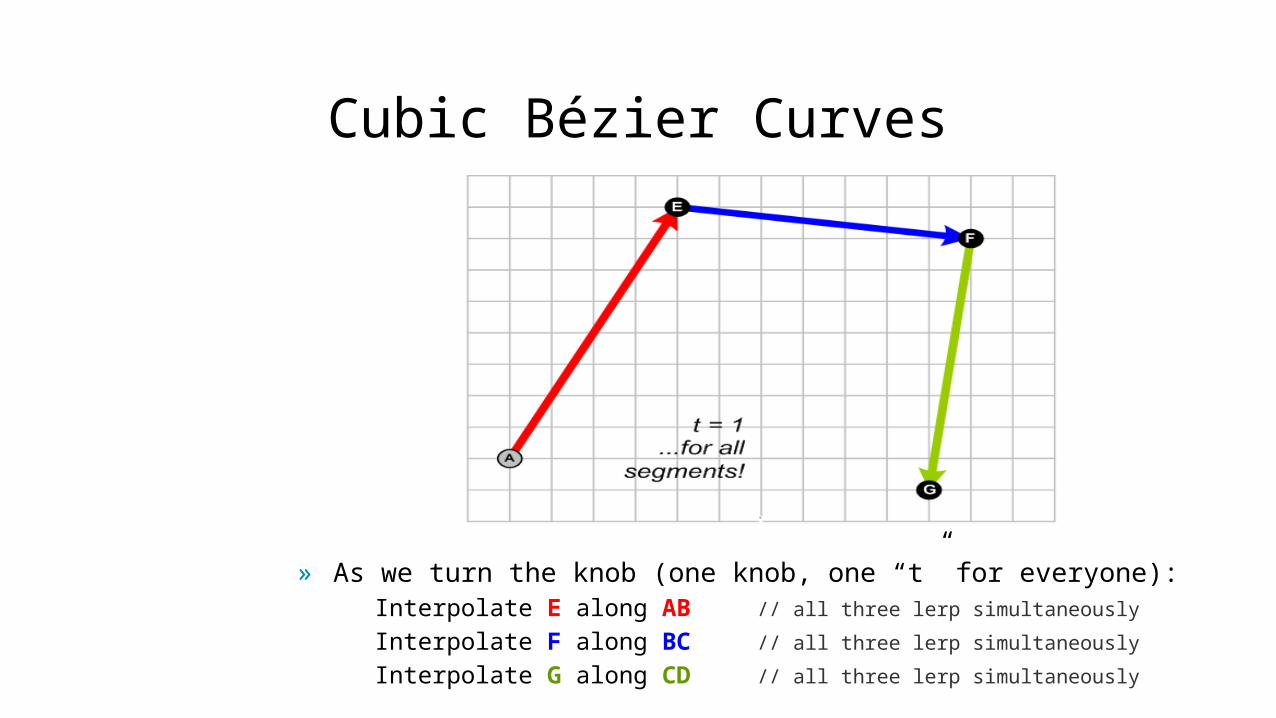
» As we turn the knob (one knob, one “t” for everyone): Interpolate E along AB // all three lerp simultaneously Interpolate F along BC // all three lerp simultaneously Interpolate G along CD // all three lerp simultaneously

Cubic Bézier Curves
» As we turn the knob (one knob, one “t” for everyone): Interpolate E along AB // all three lerp simultaneously Interpolate F along BC // all three lerp simultaneously Interpolate G along CD // all three lerp simultaneously
Cubic Bézier Curves
» As we turn the knob (one knob, one “t” for everyone): Interpolate E along AB // all three lerp simultaneously Interpolate F along BC // all three lerp simultaneously Interpolate G along CD // all three lerp simultaneously
Cubic Bézier Curves
» As we turn the knob (one knob, one “t” for everyone): Interpolate E along AB // all three lerp simultaneously Interpolate F along BC // all three lerp simultaneously Interpolate G along CD // all three lerp simultaneously
Cubic Bézier Curves
» As we turn the knob (one knob, one “t” for everyone): Interpolate E along AB // all three lerp simultaneously Interpolate F along BC // all three lerp simultaneously Interpolate G along CD // all three lerp simultaneously
Cubic Bézier Curves
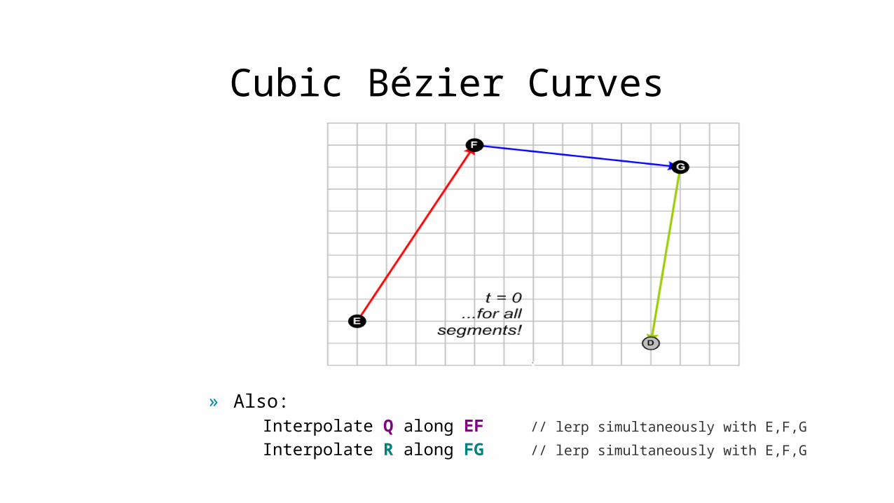
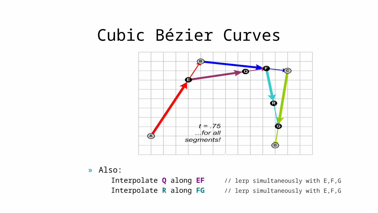
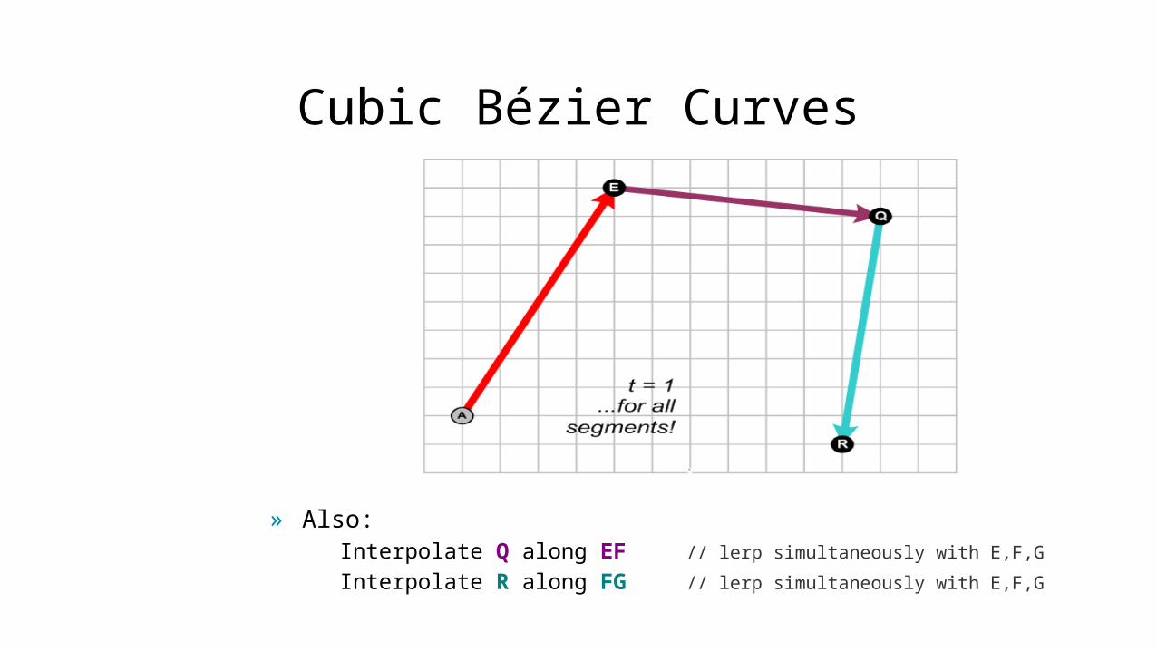
» Also: Interpolate Q along EF // lerp simultaneously with E,F,G Interpolate R along FG // lerp simultaneously with E,F,G

Cubic Bézier Curves
» Also: Interpolate Q along EF // lerp simultaneously with E,F,G Interpolate R along FG // lerp simultaneously with E,F,G

Cubic Bézier Curves
» Also: Interpolate Q along EF // lerp simultaneously with E,F,G Interpolate R along FG // lerp simultaneously with E,F,G
Cubic Bézier Curves
» Also: Interpolate Q along EF // lerp simultaneously with E,F,G Interpolate R along FG // lerp simultaneously with E,F,G
Cubic Bézier Curves
» Also: Interpolate Q along EF // lerp simultaneously with E,F,G Interpolate R along FG // lerp simultaneously with E,F,G

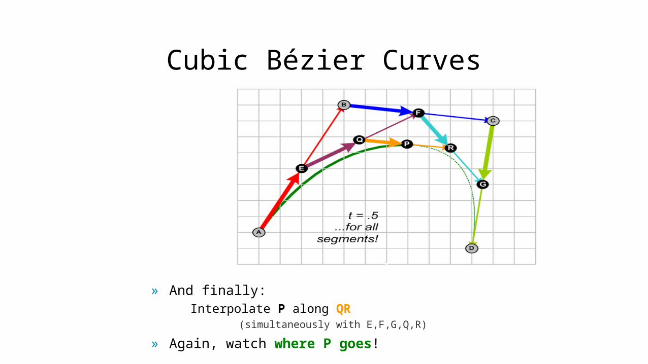
Cubic Bézier Curves
» And finally: Interpolate P along QR
(simultaneously with E,F,G,Q,R)
» Again, watch where P goes!

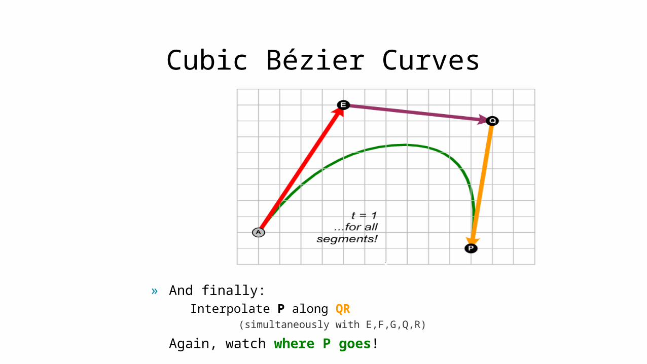
Cubic Bézier Curves
» And finally: Interpolate P along QR
(simultaneously with E,F,G,Q,R)
» Again, watch where P goes!
Cubic Bézier Curves
» And finally: Interpolate P along QR
(simultaneously with E,F,G,Q,R)
» Again, watch where P goes!

Cubic Bézier Curves
» And finally: Interpolate P along QR
(simultaneously with E,F,G,Q,R)
» Again, watch where P goes!
Cubic Bézier Curves
» And finally: Interpolate P along QR
(simultaneously with E,F,G,Q,R)
Again, watch where P goes!

Cubic Bézier Curves
A
B C
D
» Now P starts at A, and ends at D» It never touches B or C...
so they are guide points
Cubic Bézier Curves
» Remember:
A Cubic Bezier curve is justa blend of two Quadratic Bezier curves.
...which are just a blend of 3 Linear Bezier curves.
So the math is still not too bad.
(A blend of... blends of... Linear Bezier equations.)
Cubic Bézier Curves
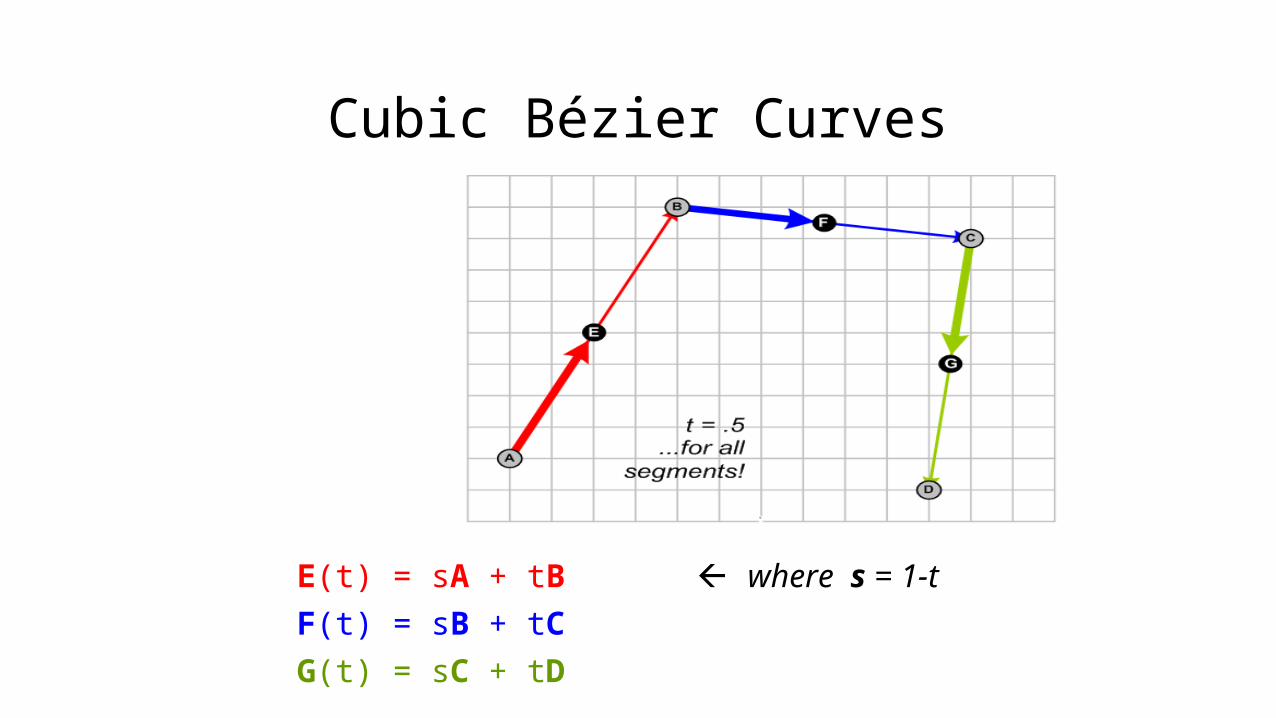
E(t) = sA + tB where s = 1-t
F(t) = sB + tC
G(t) = sC + tD

Cubic Bézier Curves
And then Q and R interpolate those results...
Q(t) = sE + tF
R(t) = sF + tG
Cubic Bézier Curves
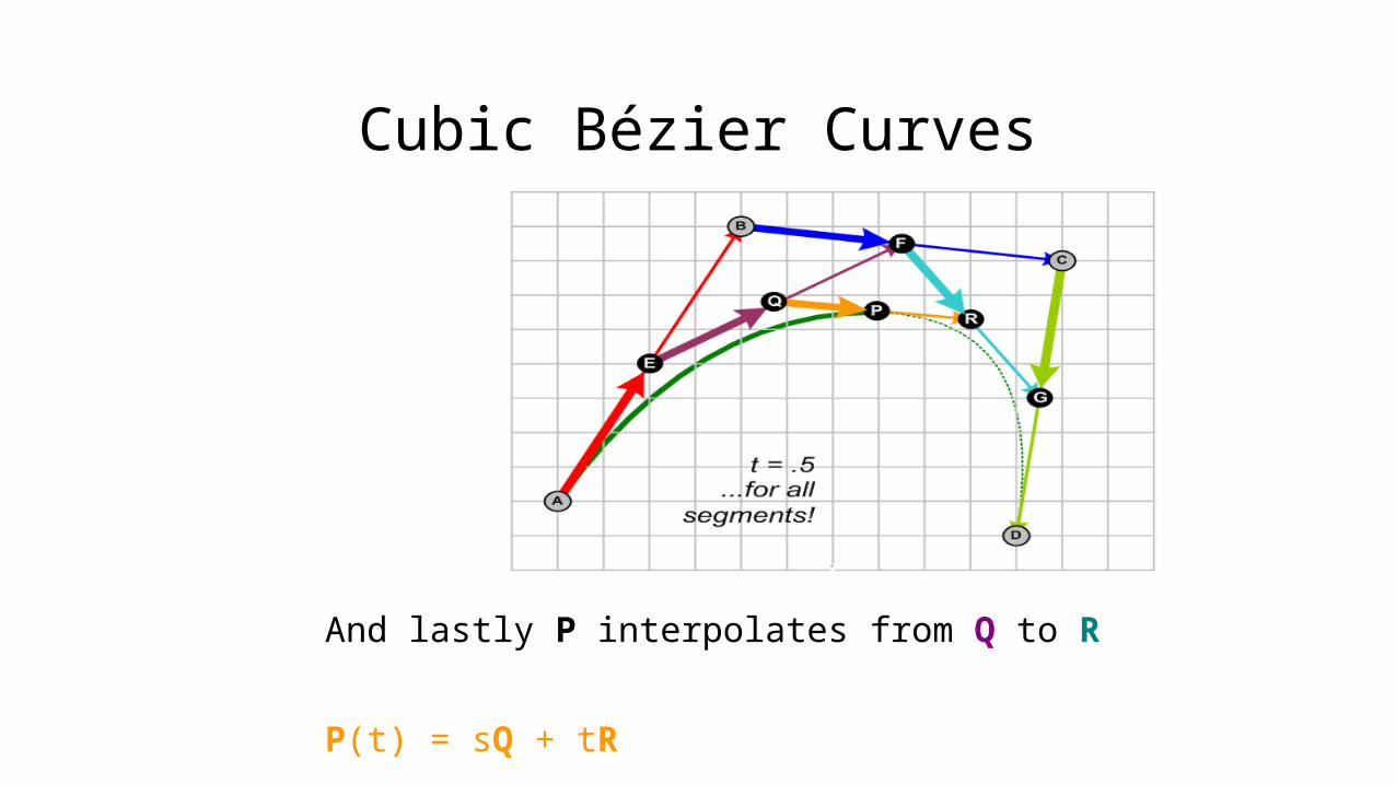
And lastly P interpolates from Q to R
P(t) = sQ + tR
Cubic Bézier Curves
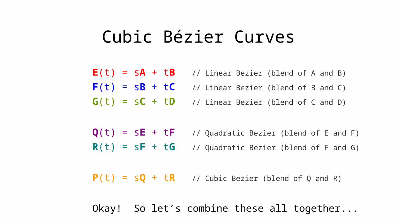
E(t) = sA + tB // Linear Bezier (blend of A and B)
F(t) = sB + tC // Linear Bezier (blend of B and C)
G(t) = sC + tD // Linear Bezier (blend of C and D)
Q(t) = sE + tF // Quadratic Bezier (blend of E and F)
R(t) = sF + tG // Quadratic Bezier (blend of F and G)
P(t) = sQ + tR // Cubic Bezier (blend of Q and R)
Okay! So let’s combine these all together...

Cubic Bézier Curves
Do some hand-waving mathemagic here......and we get one equation to rule them
all:
P(t) = (s3)A + 3(s2t)B + 3(st2)C + (t3)D
(BTW, there’s our “cubic” t3)
Cubic Bézier Curves
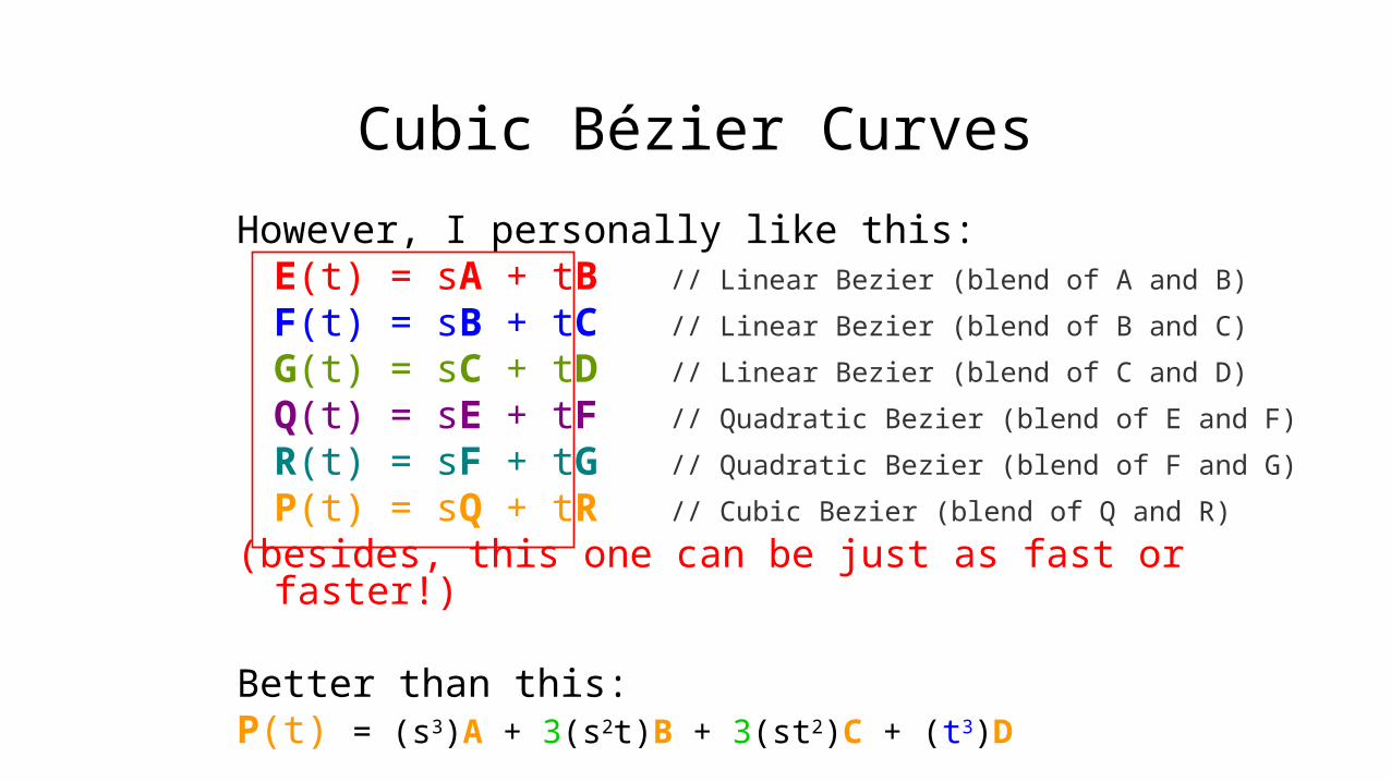
However, I personally like this:E(t) = sA + tB // Linear Bezier (blend of A and B)
F(t) = sB + tC // Linear Bezier (blend of B and C)
G(t) = sC + tD // Linear Bezier (blend of C and D)
Q(t) = sE + tF // Quadratic Bezier (blend of E and F)
R(t) = sF + tG // Quadratic Bezier (blend of F and G)
P(t) = sQ + tR // Cubic Bezier (blend of Q and R)
(besides, this one can be just as fast or faster!)
Better than this:P(t) = (s3)A + 3(s2t)B + 3(st2)C + (t3)D
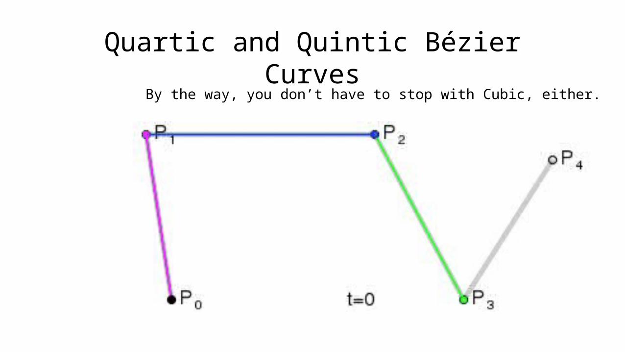
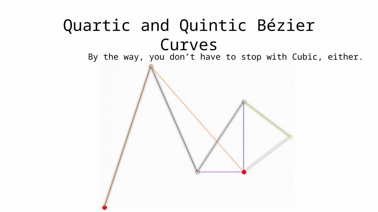
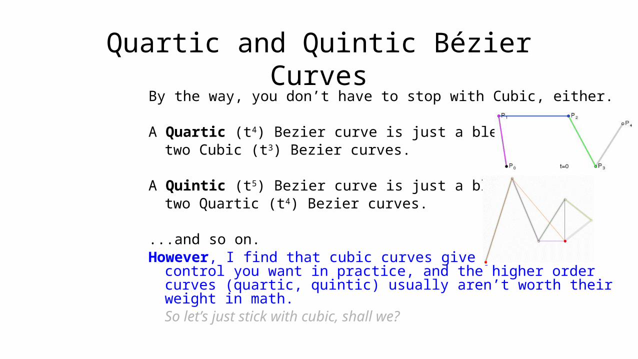
Quartic and Quintic Bézier CurvesBy the way, you don’t have to stop with Cubic, either.
A Quartic (t4) Bezier curve is just a blend oftwo Cubic (t3) Bezier curves.
A Quintic (t5) Bezier curve is just a blend oftwo Quartic (t4) Bezier curves.
...and so on.However, I find that cubic curves give you all the control
you want in practice, and the higher order curves (quartic, quintic) usually aren’t worth their weight in math.
So let’s just stick with cubic, shall we?
Cubic Bézier Curves
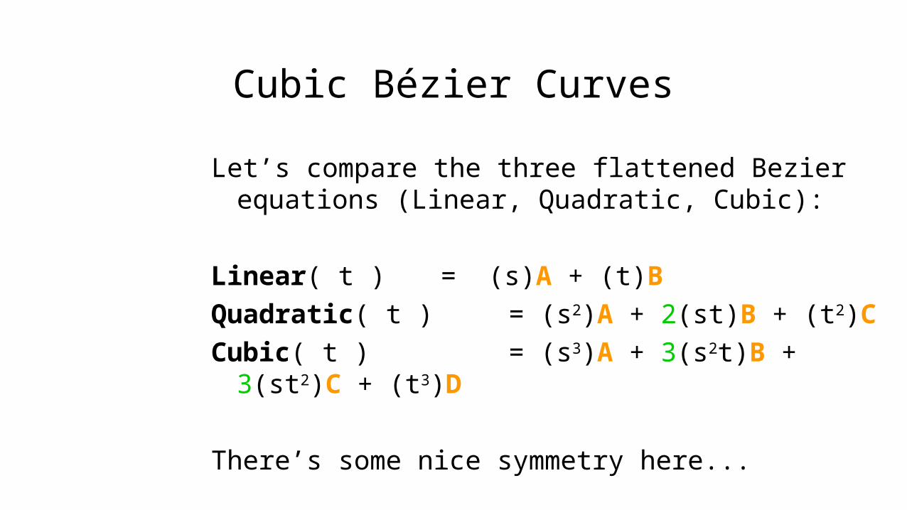
Let’s compare the three flattened Bezier equations (Linear, Quadratic, Cubic):
Linear( t ) = (s)A + (t)BQuadratic( t ) = (s2)A + 2(st)B + (t2)CCubic( t ) = (s3)A + 3(s2t)B + 3(st2)C +
(t3)D
There’s some nice symmetry here...
Cubic Bézier Curves
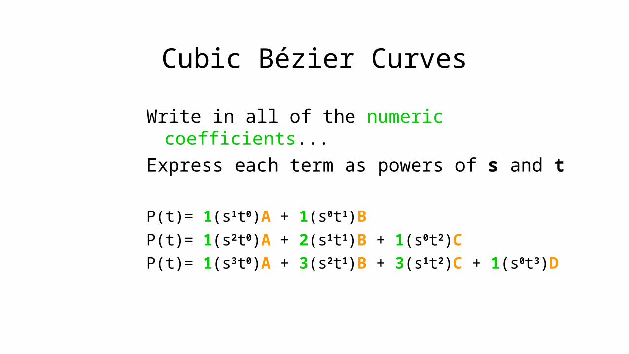
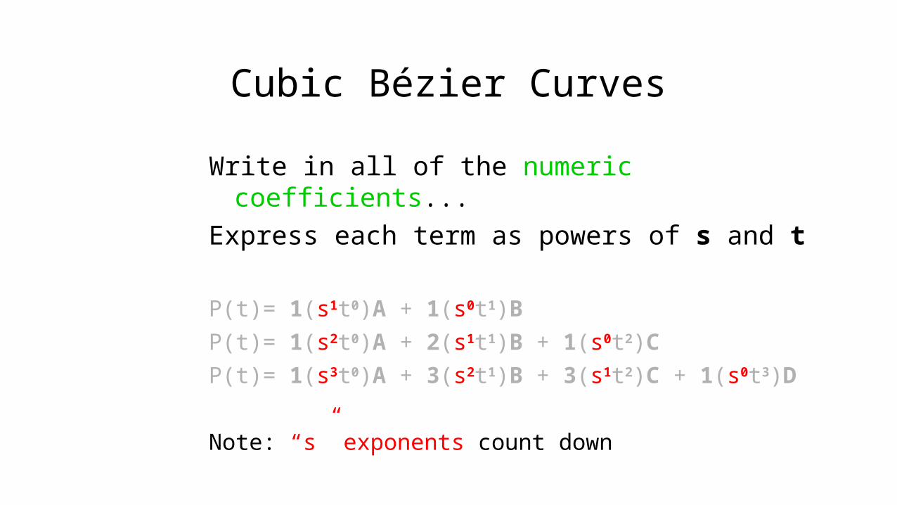
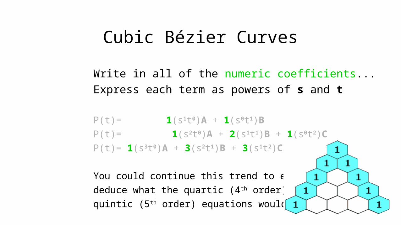
Write in all of the numeric coefficients...Express each term as powers of s and t
P(t)= 1(s1t0)A + 1(s0t1)B
P(t)= 1(s2t0)A + 2(s1t1)B + 1(s0t2)C
P(t)= 1(s3t0)A + 3(s2t1)B + 3(s1t2)C + 1(s0t3)D
Cubic Bézier Curves
Write in all of the numeric coefficients...Express each term as powers of s and t
P(t)= 1(s1t0)A + 1(s0t1)B
P(t)= 1(s2t0)A + 2(s1t1)B + 1(s0t2)C
P(t)= 1(s3t0)A + 3(s2t1)B + 3(s1t2)C + 1(s0t3)D
Note: “s” exponents count down
Cubic Bézier Curves
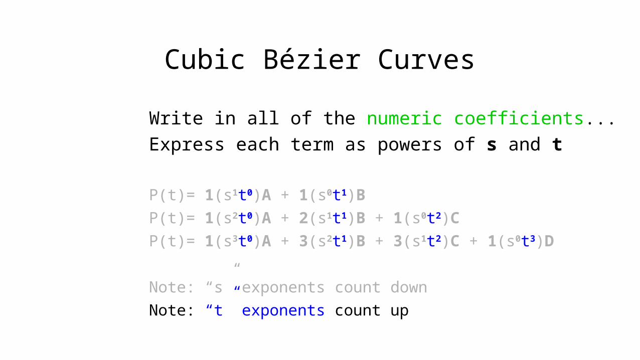
Write in all of the numeric coefficients...Express each term as powers of s and t
P(t)= 1(s1t0)A + 1(s0t1)B
P(t)= 1(s2t0)A + 2(s1t1)B + 1(s0t2)C
P(t)= 1(s3t0)A + 3(s2t1)B + 3(s1t2)C + 1(s0t3)D
Note: “s” exponents count down
Note: “t” exponents count up
Cubic Bézier Curves
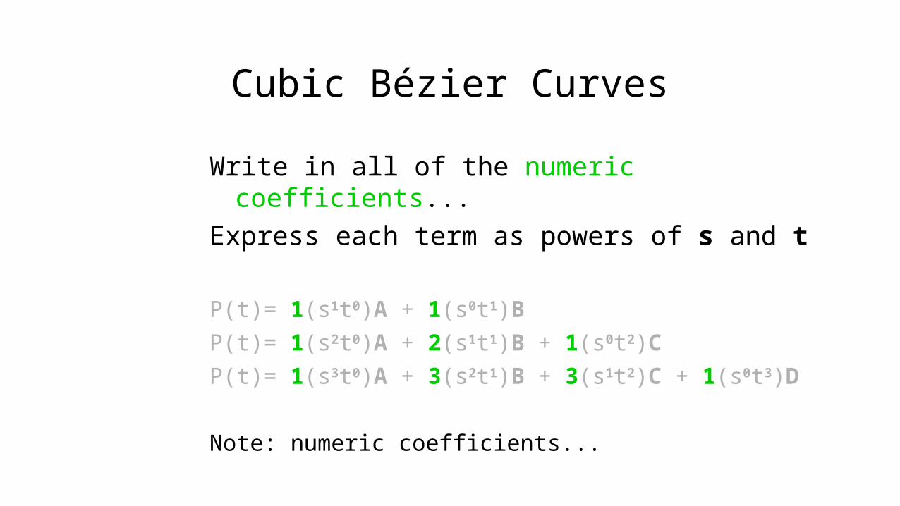
Write in all of the numeric coefficients...Express each term as powers of s and t
P(t)= 1(s1t0)A + 1(s0t1)B
P(t)= 1(s2t0)A + 2(s1t1)B + 1(s0t2)C
P(t)= 1(s3t0)A + 3(s2t1)B + 3(s1t2)C + 1(s0t3)D
Note: numeric coefficients...
Cubic Bézier Curves
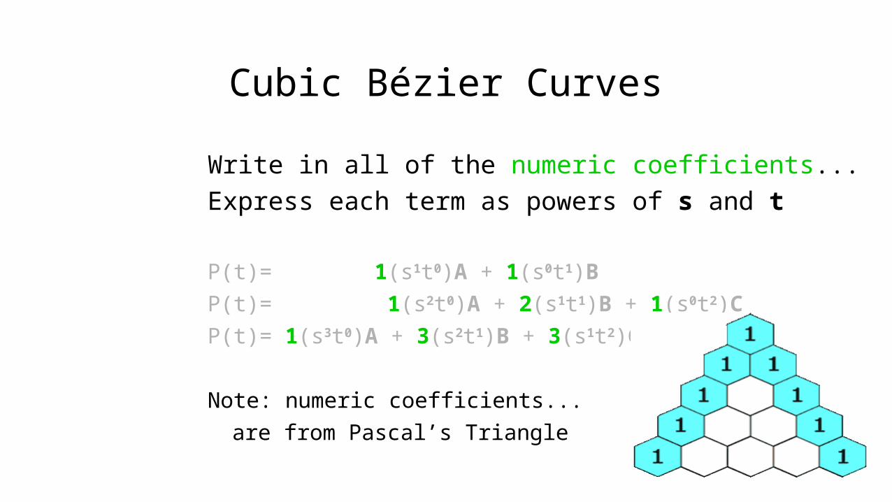
Write in all of the numeric coefficients...Express each term as powers of s and t
P(t)= 1(s1t0)A + 1(s0t1)B
P(t)= 1(s2t0)A + 2(s1t1)B + 1(s0t2)C
P(t)= 1(s3t0)A + 3(s2t1)B + 3(s1t2)C + 1(s0t3)D
Note: numeric coefficients...
are from Pascal’s Triangle
Cubic Bézier Curves
Write in all of the numeric coefficients...Express each term as powers of s and t
P(t)= 1(s1t0)A + 1(s0t1)B
P(t)= 1(s2t0)A + 2(s1t1)B + 1(s0t2)C
P(t)= 1(s3t0)A + 3(s2t1)B + 3(s1t2)C + 1(s0t3)D
You could continue this trend to easily
deduce what the quartic (4th order) and
quintic (5th order) equations would be...
Cubic Bézier Curves
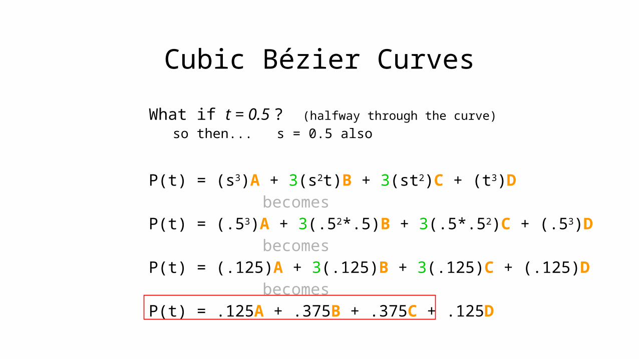
What if t = 0.5 ? (halfway through the curve)
so then... s = 0.5 also
P(t) = (s3)A + 3(s2t)B + 3(st2)C + (t3)Dbecomes
P(t) = (.53)A + 3(.52*.5)B + 3(.5*.52)C + (.53)Dbecomes
P(t) = (.125)A + 3(.125)B + 3(.125)C + (.125)Dbecomes
P(t) = .125A + .375B + .375C + .125D
Cubic Bézier Curves
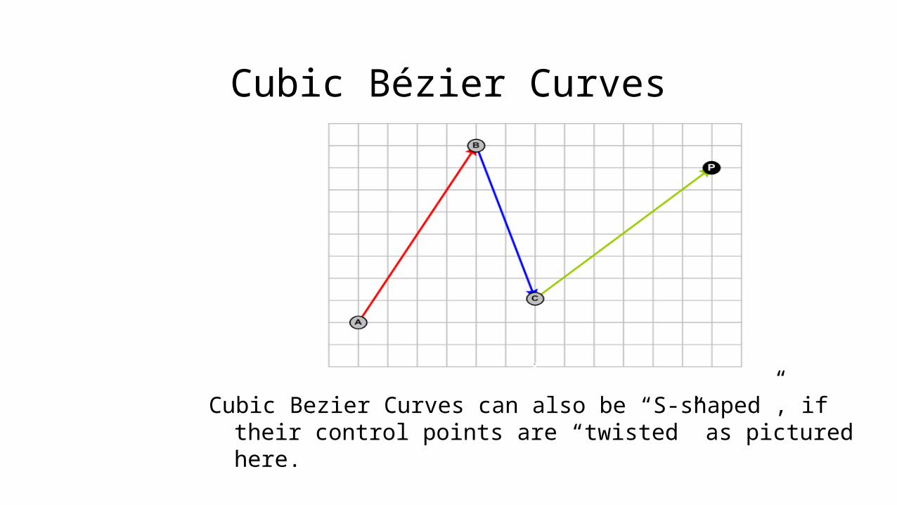
Cubic Bezier Curves can also be “S-shaped”, if their control points are “twisted” as pictured here.
Cubic Bézier Curves
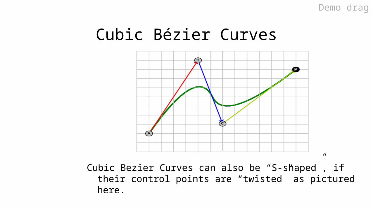
Cubic Bezier Curves can also be “S-shaped”, if their control points are “twisted” as pictured here.
Demo drag
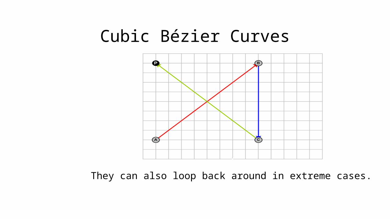
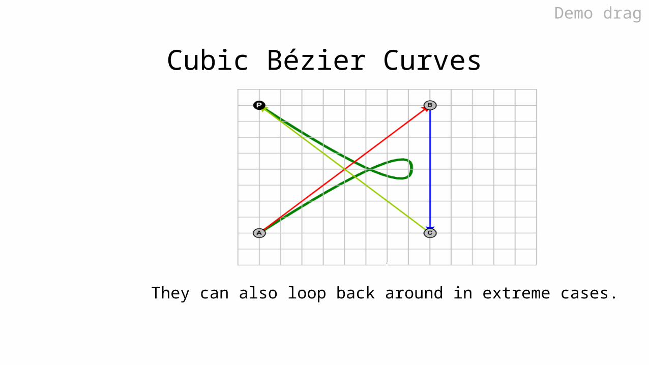
Cubic Bézier Curves
They can also loop back around in extreme cases.
Cubic Bézier Curves
They can also loop back around in extreme cases.
Demo drag

Seen in lots of places:
» Photoshop» GIMP» PostScript» Flash» AfterEffects» 3DS Max» Metafont
» Understable Disc Golf flight path
Cubic Bézier Curves
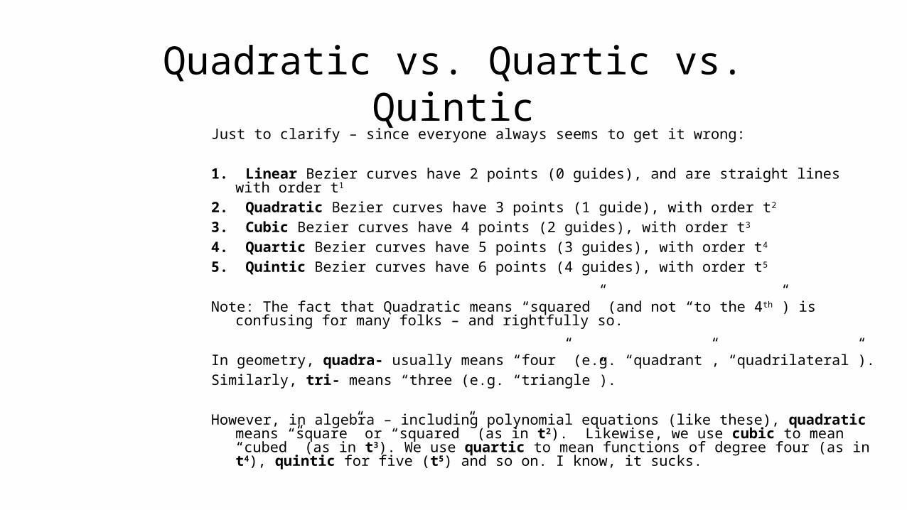
Quadratic vs. Quartic vs. QuinticJust to clarify – since everyone always seems to get it wrong:
1. Linear Bezier curves have 2 points (0 guides), and are straight lines with order t1
2. Quadratic Bezier curves have 3 points (1 guide), with order t2
3. Cubic Bezier curves have 4 points (2 guides), with order t3
4. Quartic Bezier curves have 5 points (3 guides), with order t4
5. Quintic Bezier curves have 6 points (4 guides), with order t5
Note: The fact that Quadratic means “squared” (and not “to the 4th”) is confusing for many folks – and rightfully so.
In geometry, quadra- usually means “four” (e.g. “quadrant”, “quadrilateral”).Similarly, tri- means “three (e.g. “triangle”).
However, in algebra – including polynomial equations (like these), quadratic means “square” or “squared” (as in t2). Likewise, we use cubic to mean “cubed” (as in t3). We use quartic to mean functions of degree four (as in t4), quintic for five (t5) and so on. I know, it sucks.

Splines

Splines
Okay, enough of Curves already.
So... what’s a Spline?

Splines
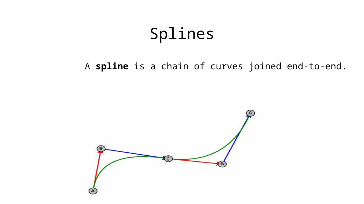
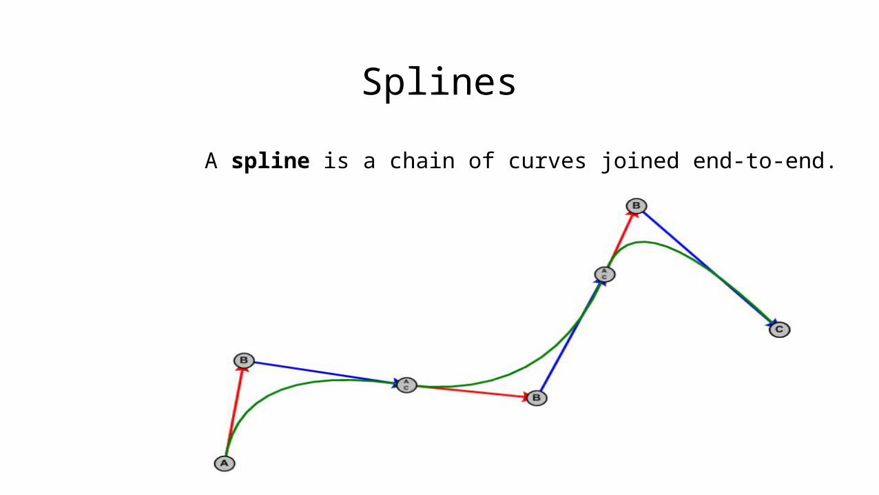
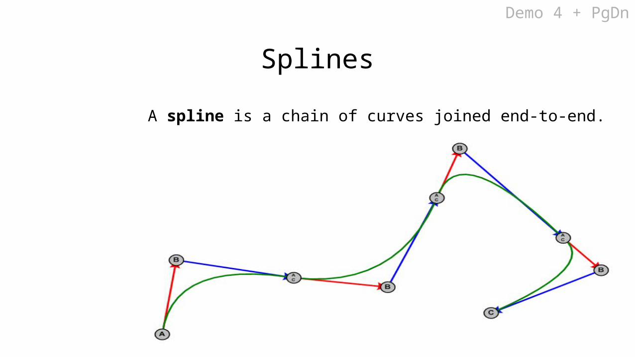
A spline is a chain of curves joined end-to-end.
Splines
A spline is a chain of curves joined end-to-end.
Splines
A spline is a chain of curves joined end-to-end.
Splines
A spline is a chain of curves joined end-to-end.
Demo 4 + PgDn
Splines
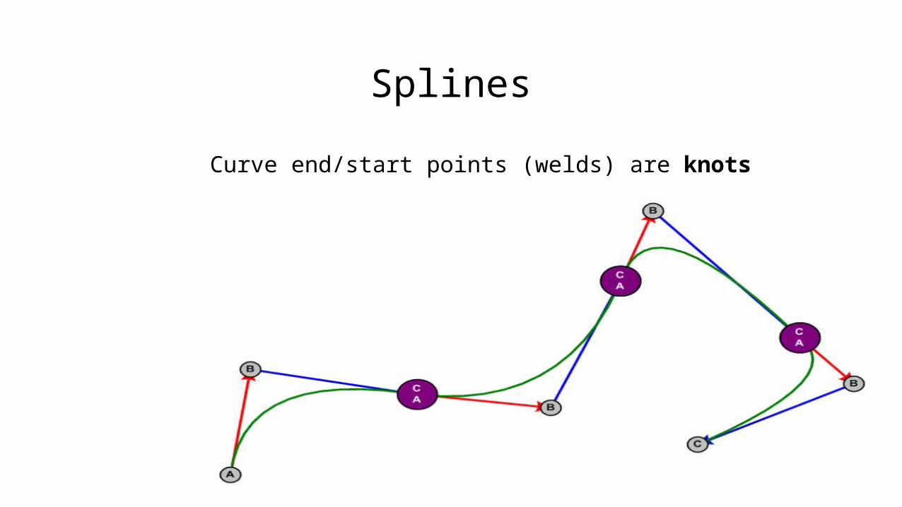
Curve end/start points (welds) are knots
Splines
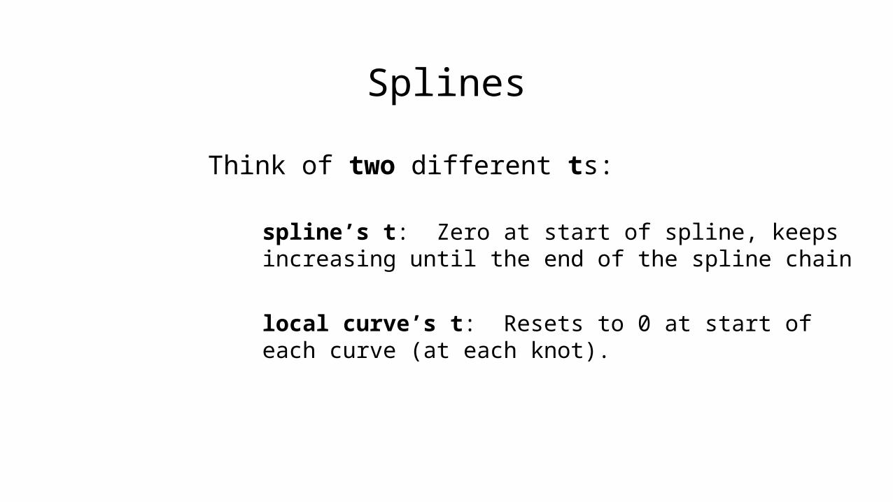
Think of two different ts:
spline’s t: Zero at start of spline, keeps increasing until the end of the spline chain
local curve’s t: Resets to 0 at start of each curve (at each knot).

Splines
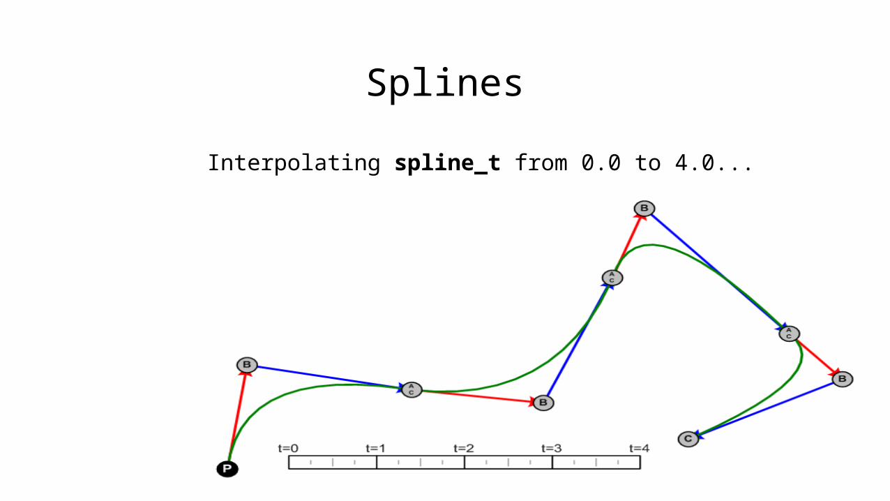
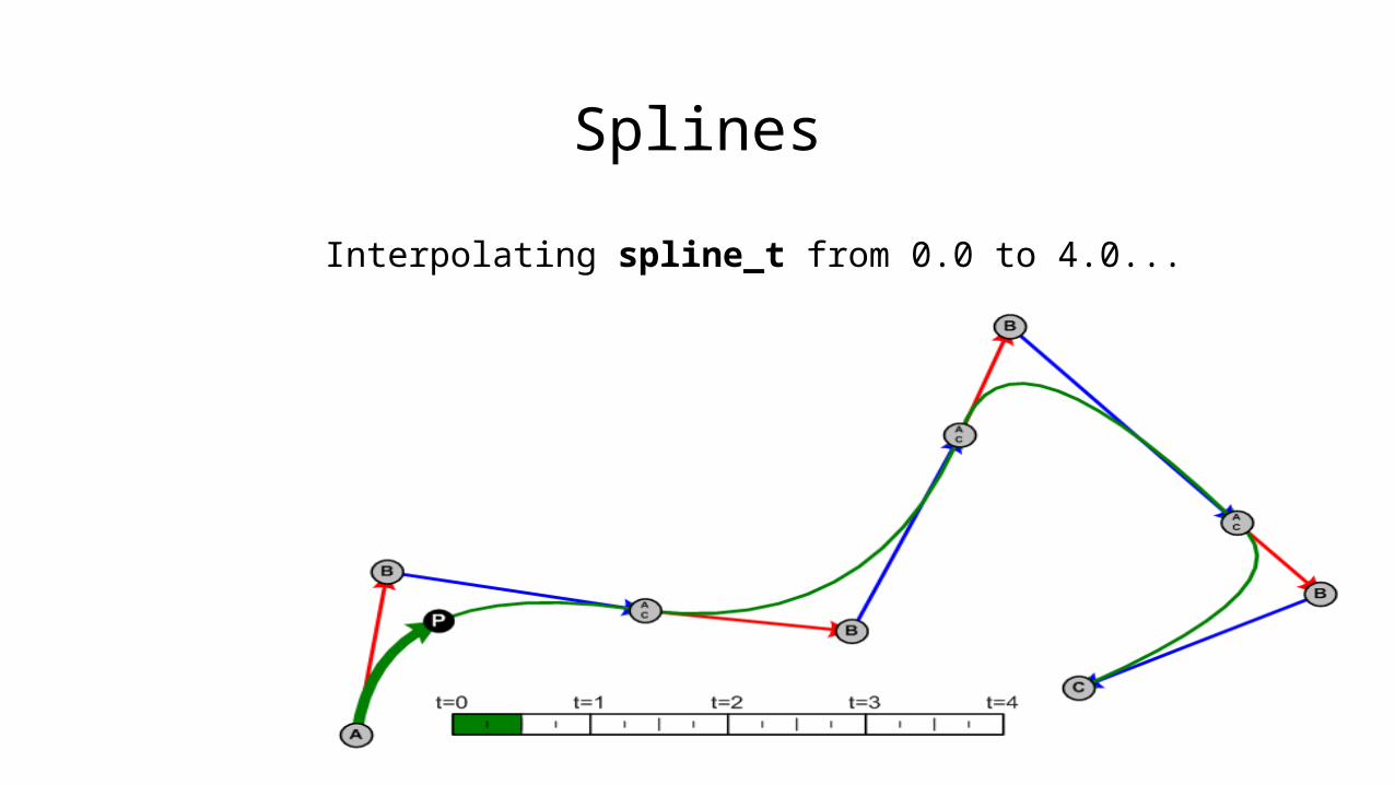
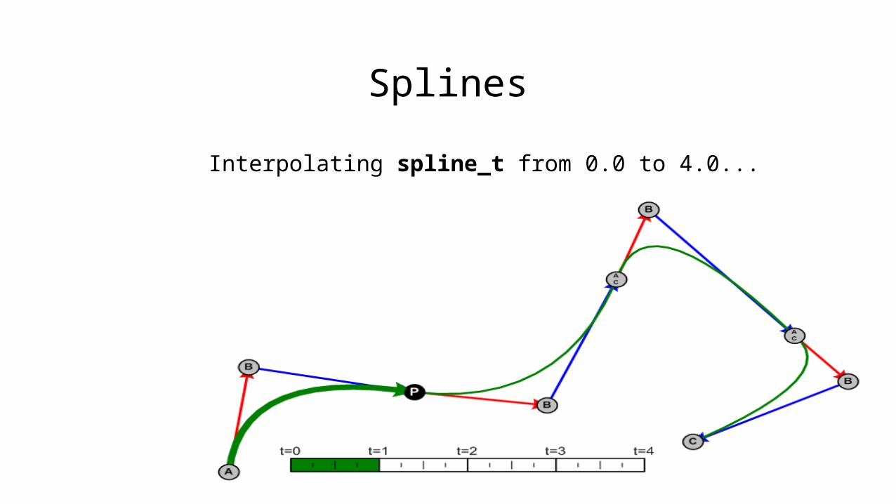
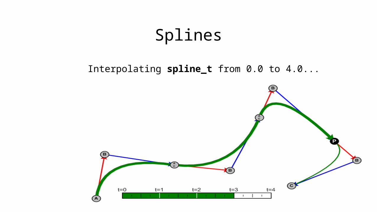
For a spline of 4 curve-pieces:
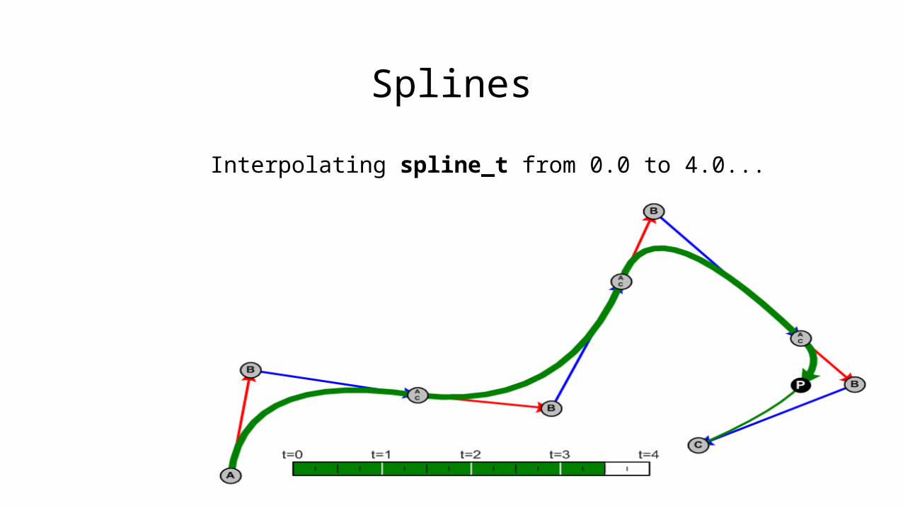
» Interpolate spline_t from 0.0 to 4.0
» If spline_t is 2.67, then we are:In the third curve section (0,1,2,3), and67% through that section (local_t = .67)
» So... plug local_t into curve[2], i.e.P( 2.67 ) = curve[2].EvaluateAt( .67 );
Splines
Interpolating spline_t from 0.0 to 4.0...
Splines
Interpolating spline_t from 0.0 to 4.0...
Splines
Interpolating spline_t from 0.0 to 4.0...

Splines
Interpolating spline_t from 0.0 to 4.0...

Splines
Interpolating spline_t from 0.0 to 4.0...

Splines
Interpolating spline_t from 0.0 to 4.0...
Splines
Interpolating spline_t from 0.0 to 4.0...
Splines
Interpolating spline_t from 0.0 to 4.0...
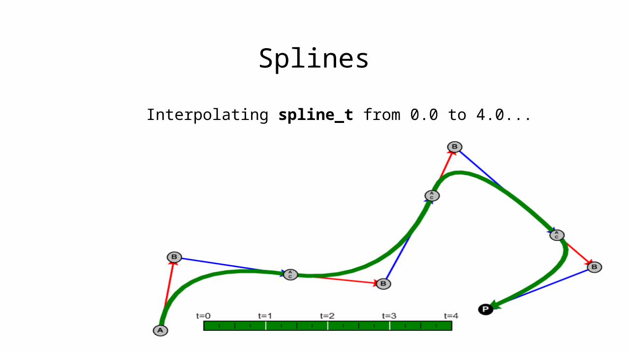
Splines
Interpolating spline_t from 0.0 to 4.0...

Quadratic Bezier Splines
This spline is a quadratic Bezier spline,
since it is a spline made out of
quadratic Bezier curves

Continuity
Good continuity (C1); connected and aligned
Poor continuity (C0); connected but not aligned

Continuity
To ensure good continuity (C1), make BC of first curve colinear (in line with) AB of second curve.
(derivative is continuous across entire spline)
Continuity
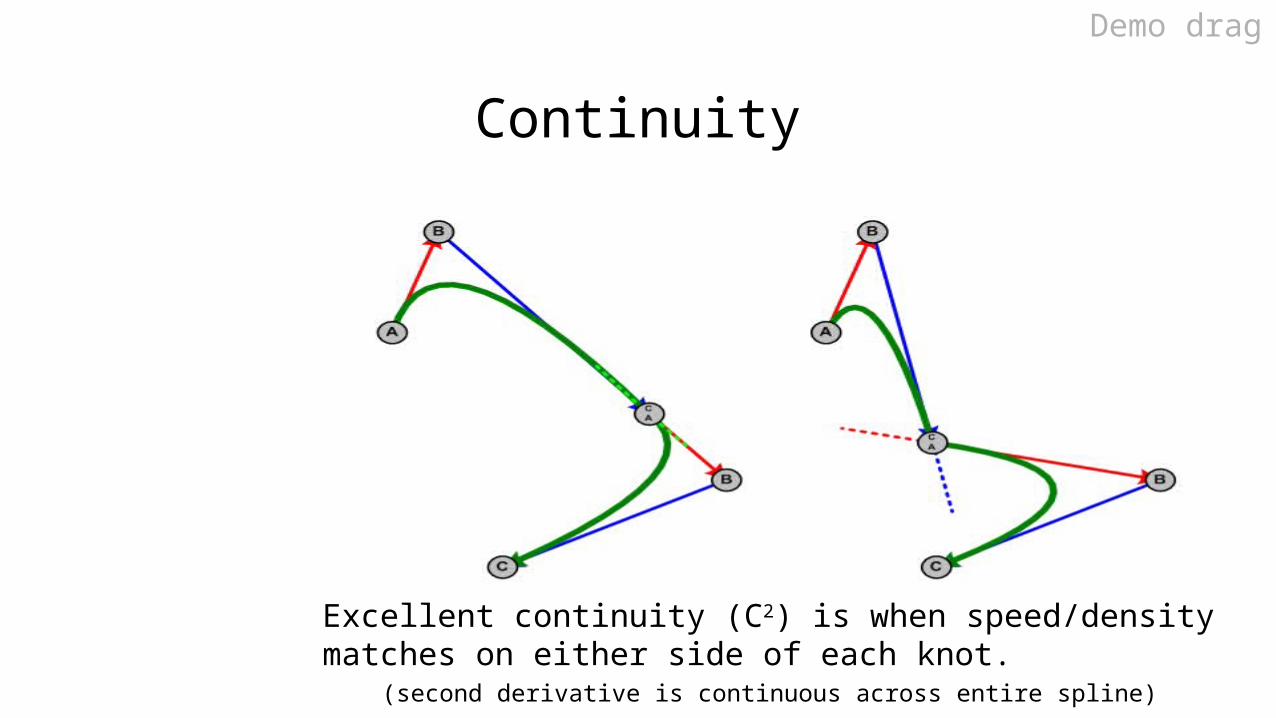
Excellent continuity (C2) is when speed/density matches on either side of each knot.
(second derivative is continuous across entire spline)
Demo drag

Cubic Bezier Splines
We can build a cubic Bezier spline instead by using cubic Bezier curves.

Cubic Bezier Splines
We can build a cubic Bezier spline instead by using cubic Bezier curves.

Cubic Bezier Splines
We can build a cubic Bezier spline instead by using cubic Bezier curves.
Demo 5+PgDn
Demo 3 (CP)
Cubic Hermite Splines
(pronounced “her-meet”)
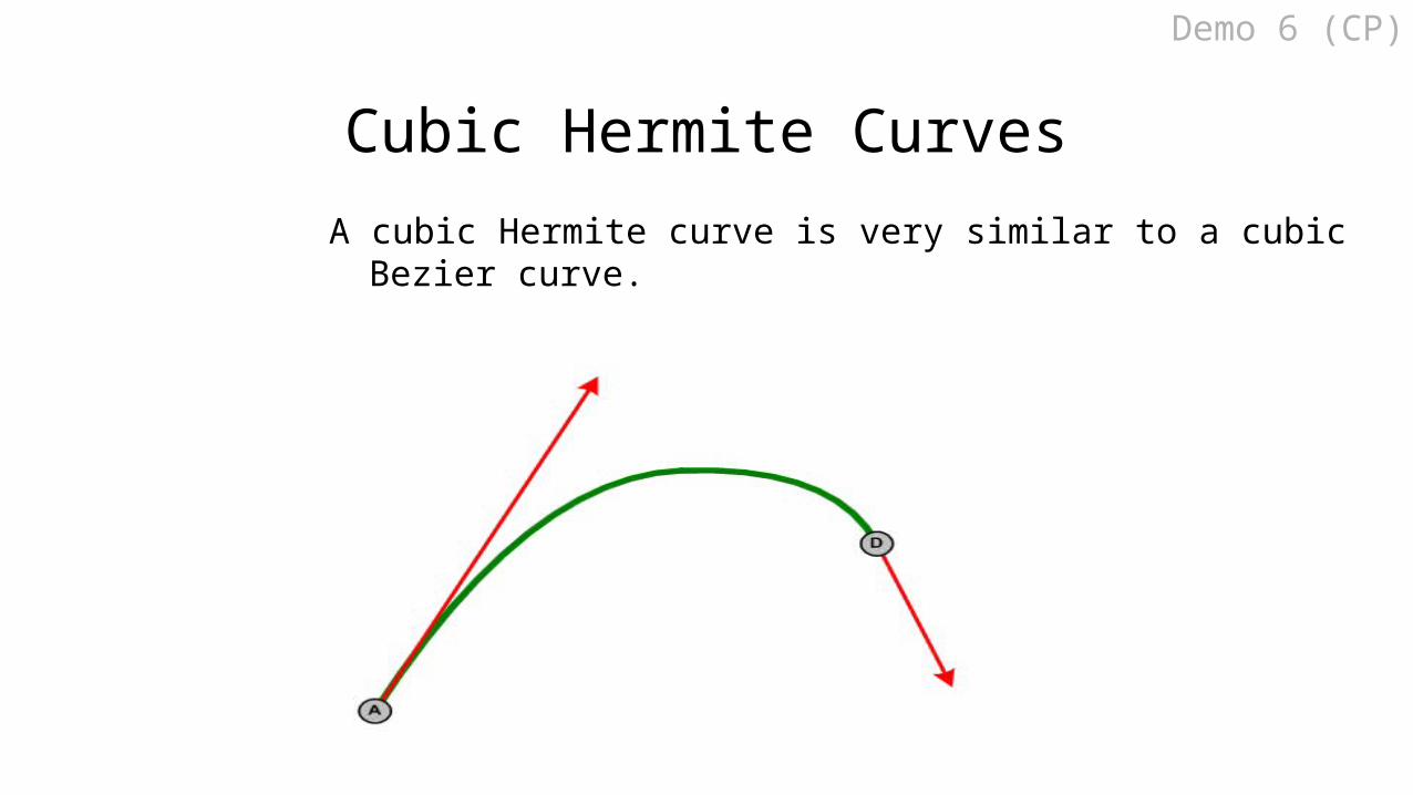
Cubic Hermite Curves
A cubic Hermite curve is very similar to a cubic Bezier curve.
Demo 6 (CP)
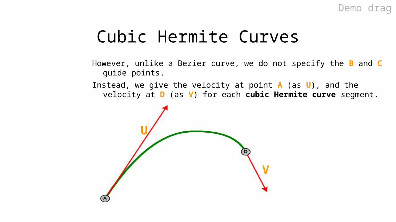
Cubic Hermite CurvesHowever, unlike a Bezier curve, we do not specify the B and C guide
points.
Instead, we give the velocity at point A (as U), and the velocity at D (as V) for each cubic Hermite curve segment.
U
V
Demo drag

Cubic Hermite SplinesTo ensure connectedness (C0), D from curve #0 is typically assumed
to be welded on top of A from curve #1 (at a knot).

Cubic Hermite SplinesTo ensure smoothness (C1), velocity into D (V) is typically assumed to
match the velocity’s direction out of the next curve’s A (U).
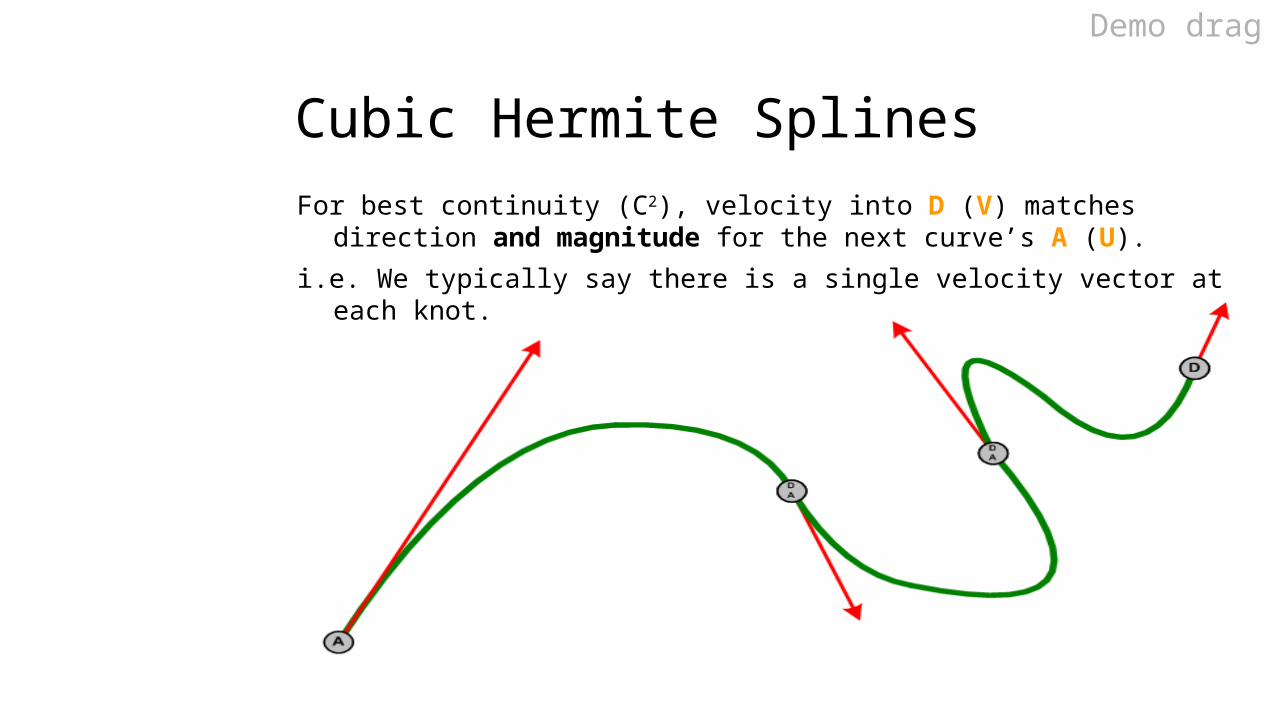
Cubic Hermite SplinesFor best continuity (C2), velocity into D (V) matches direction and
magnitude for the next curve’s A (U).
i.e. We typically say there is a single velocity vector at each knot.
Demo drag
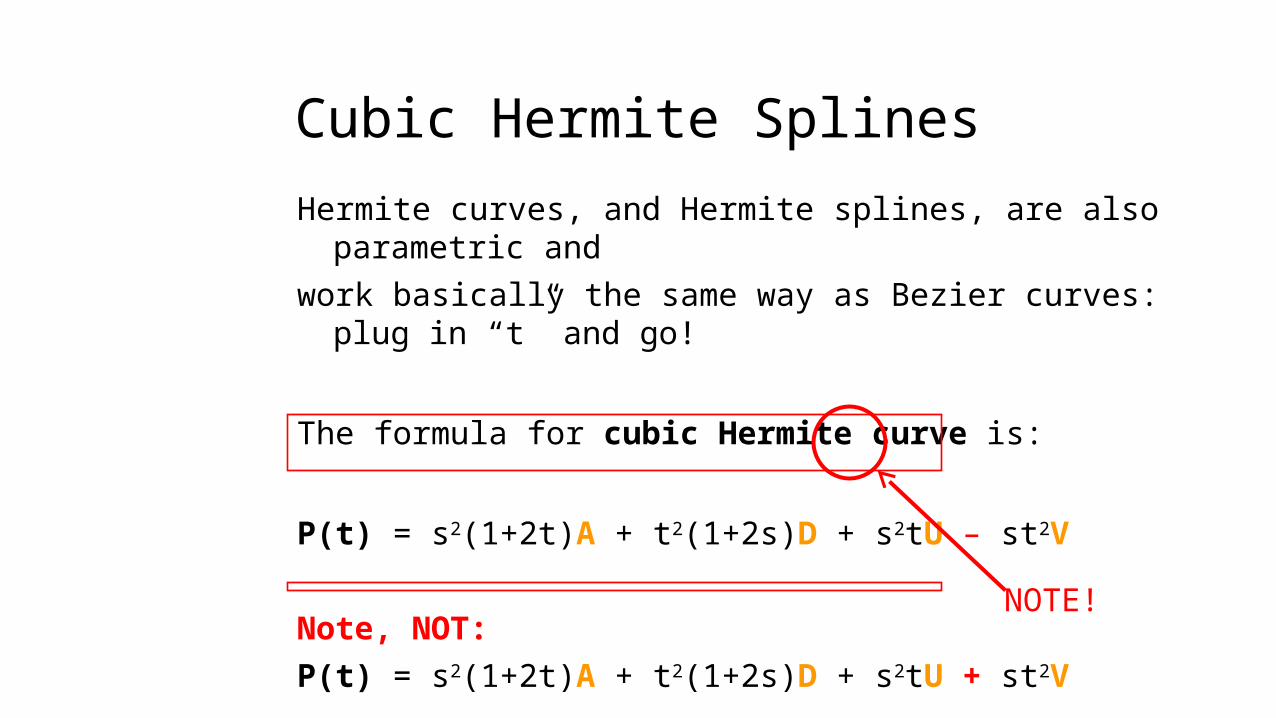
Cubic Hermite Splines
Hermite curves, and Hermite splines, are also parametric and
work basically the same way as Bezier curves: plug in “t” and go!
The formula for cubic Hermite curve is:
P(t) = s2(1+2t)A + t2(1+2s)D + s2tU – st2V
Note, NOT:
P(t) = s2(1+2t)A + t2(1+2s)D + s2tU + st2V
NOTE!
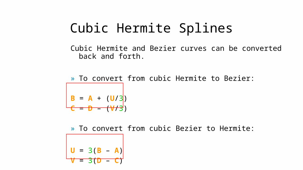
Cubic Hermite SplinesCubic Hermite and Bezier curves can be converted back
and forth.
» To convert from cubic Hermite to Bezier:
B = A + (U/3)C = D – (V/3)
» To convert from cubic Bezier to Hermite:
U = 3(B – A)V = 3(D – C)

Cubic Hermite SplinesCubic Hermite and Bezier curves can be converted back
and forth.
» To convert from cubic Hermite to Bezier:
B = A + (U/3)C = D – (V/3)
» To convert from cubic Bezier to Hermite:
U = 3(B – A)V = 3(D – C)
...and are therefore basically the exact same thing!
Catmull-Rom Splines

Catmull-Rom Splines
A Catmull-Rom spline is just a cubic Hermite spline with special values chosen for the velocities at the start (U) and end (V) points of each section.
You can also think of Catmull-Rom not as a type of spline, but as a technique for building cubic Hermite splines.
Best application: curve-pathing through points

Catmull-Rom Splines
Start with a series of points (spline start, spline end, and interior knots)

Catmull-Rom Splines
1. Assume U and V velocities are zero at start and end of spline (points 0 and 6 here).
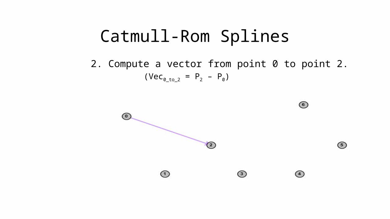
Catmull-Rom Splines
2. Compute a vector from point 0 to point 2.(Vec0_to_2 = P2 – P0)

Catmull-Rom Splines
That will be our tangent for point 1.
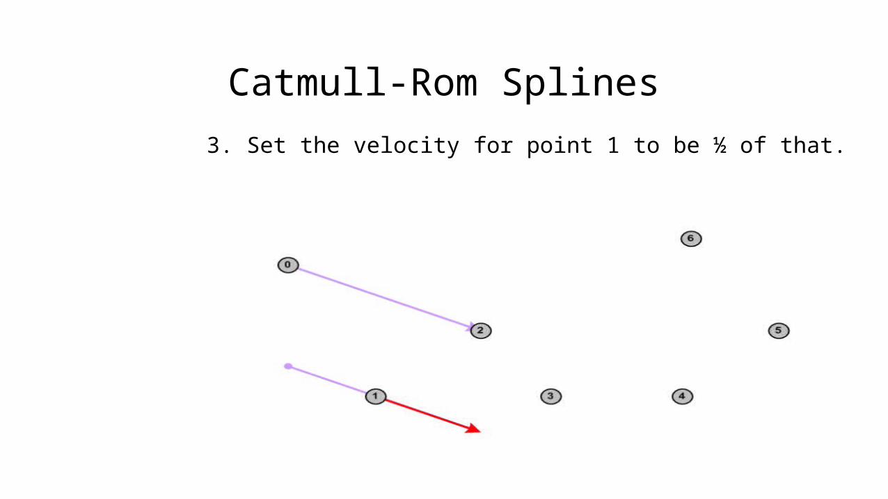
Catmull-Rom Splines
3. Set the velocity for point 1 to be ½ of that.
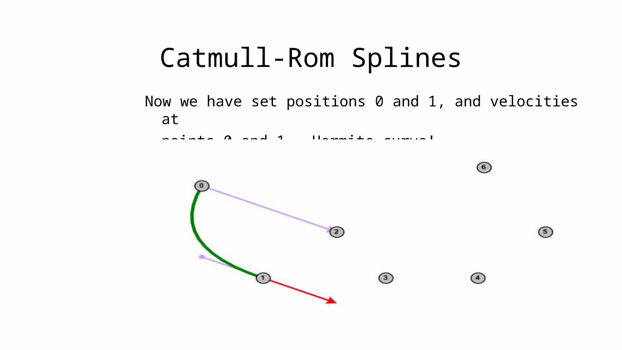
Catmull-Rom Splines
Now we have set positions 0 and 1, and velocities at
points 0 and 1. Hermite curve!
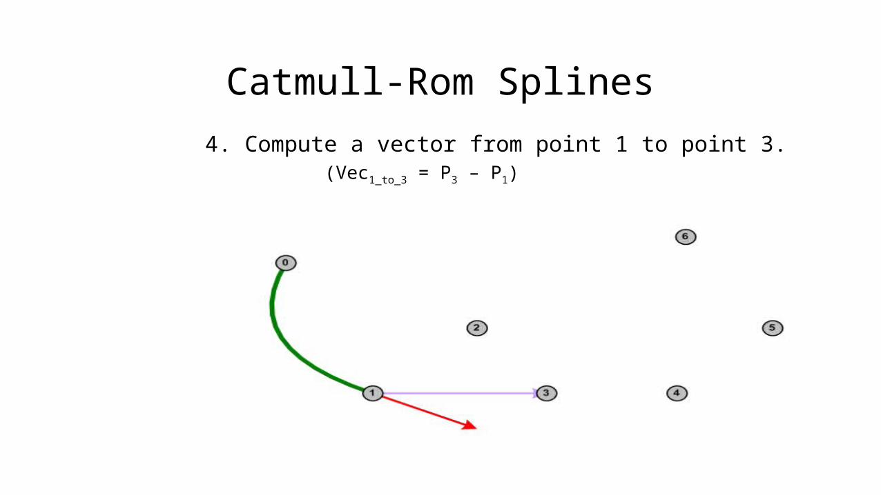
Catmull-Rom Splines
4. Compute a vector from point 1 to point 3.(Vec1_to_3 = P3 – P1)
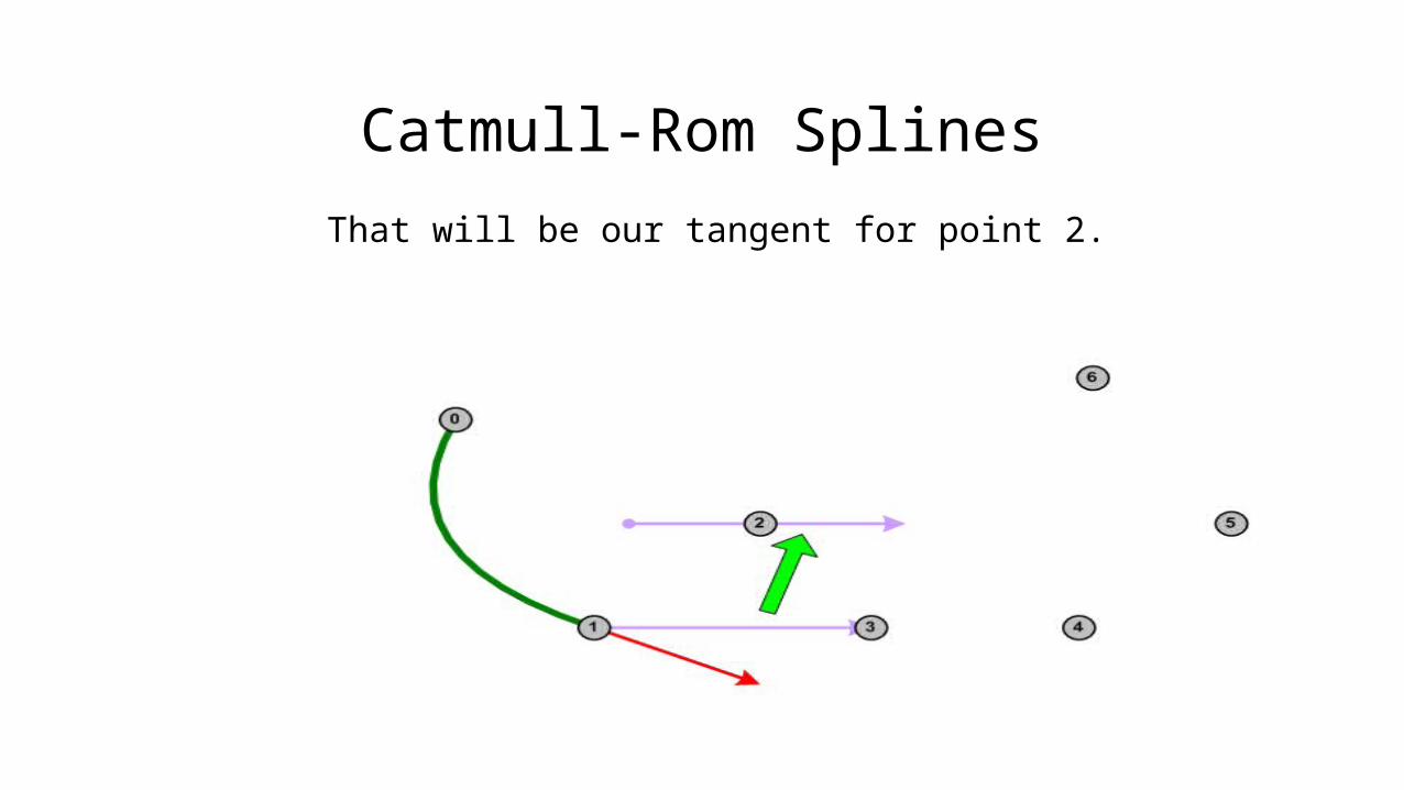
Catmull-Rom Splines
That will be our tangent for point 2.

Catmull-Rom Splines
5. Set the velocity for point 2 to be ½ of that.

Catmull-Rom Splines
Now we have set positions and velocities for points 0, 1, and 2. We have a Hermite spline!
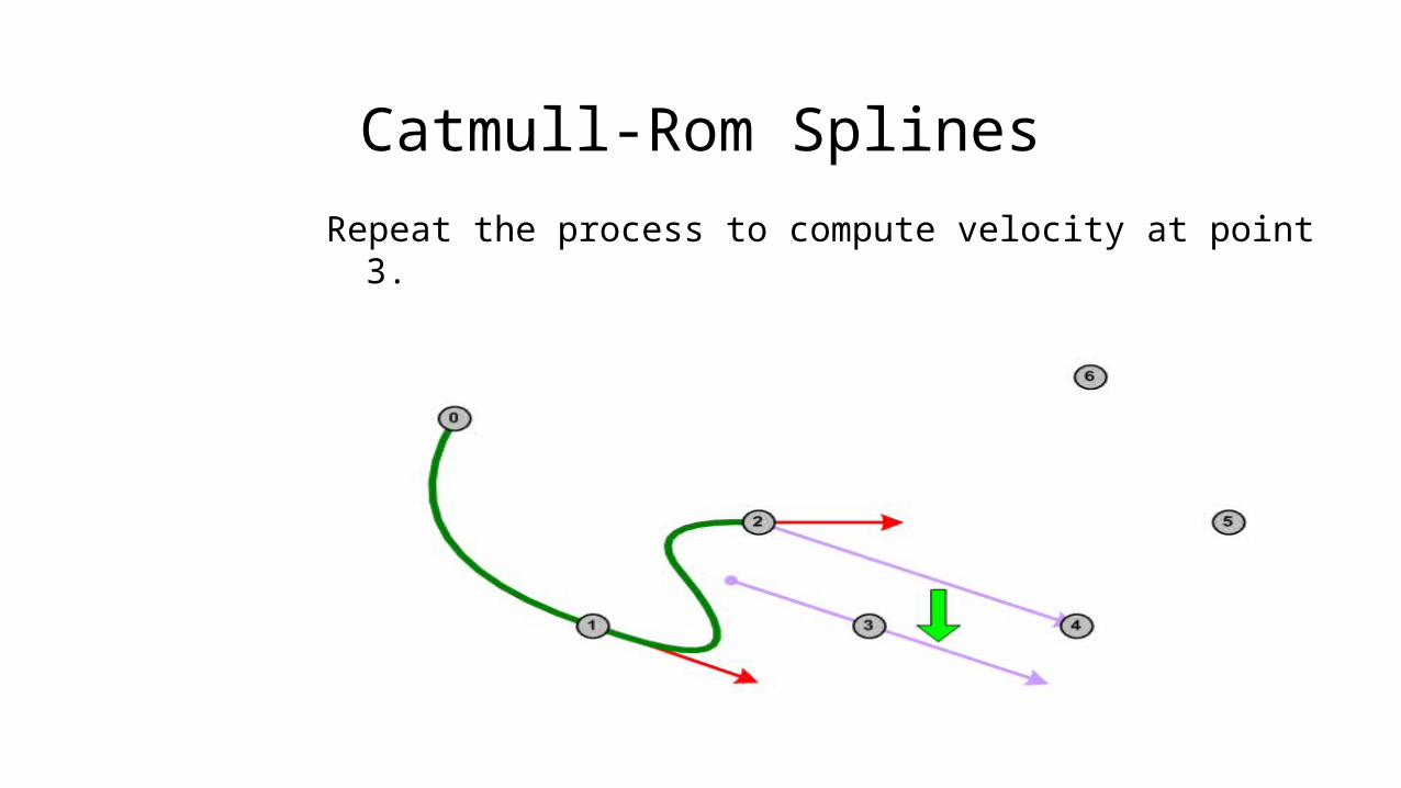
Catmull-Rom Splines
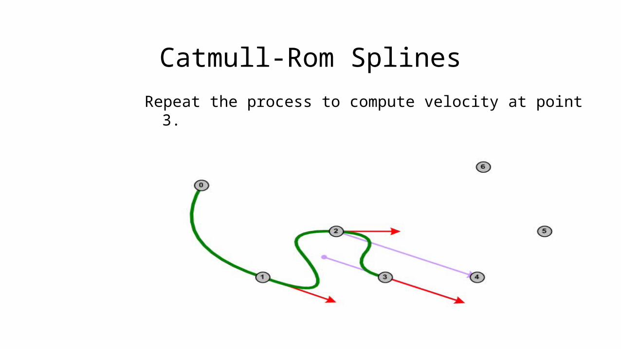
Repeat the process to compute velocity at point 3.
Catmull-Rom Splines
Repeat the process to compute velocity at point 3.

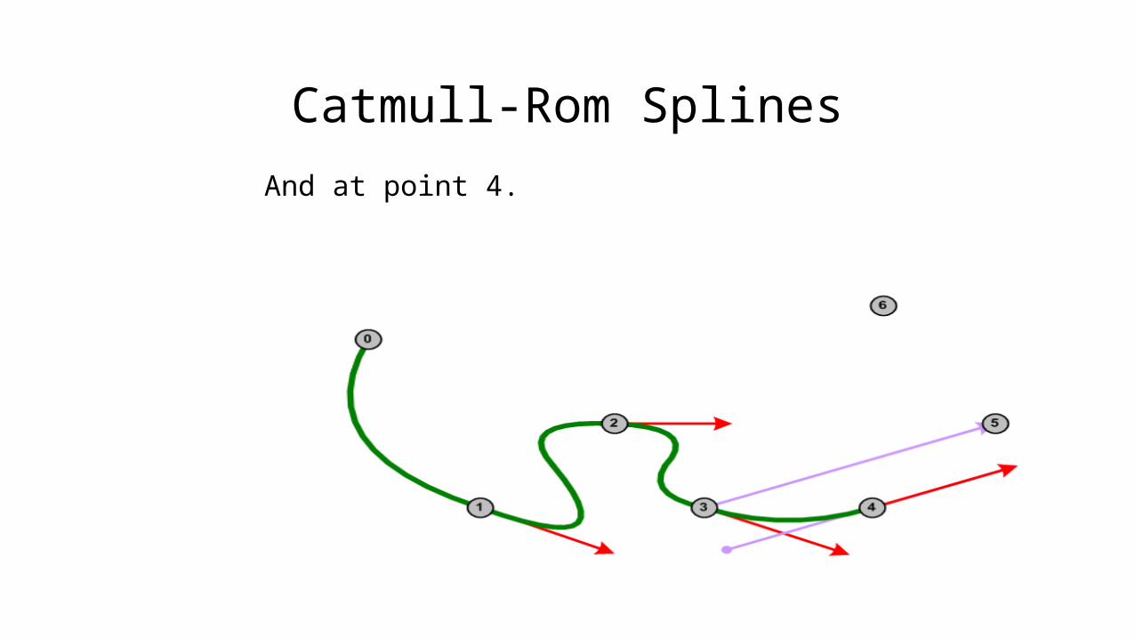
Catmull-Rom Splines
And at point 4.
Catmull-Rom Splines
And at point 4.
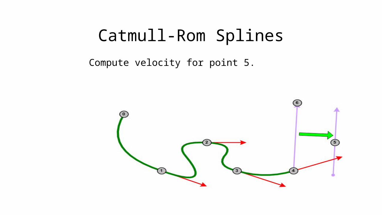
Catmull-Rom Splines
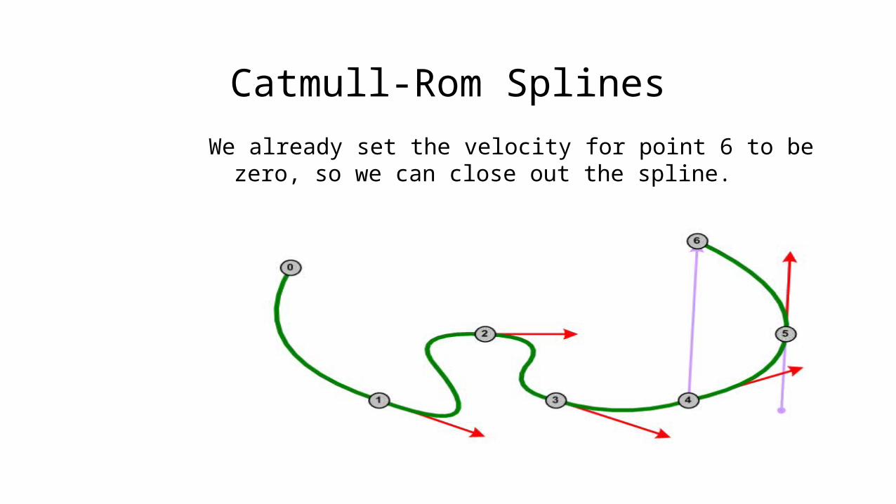
Compute velocity for point 5.
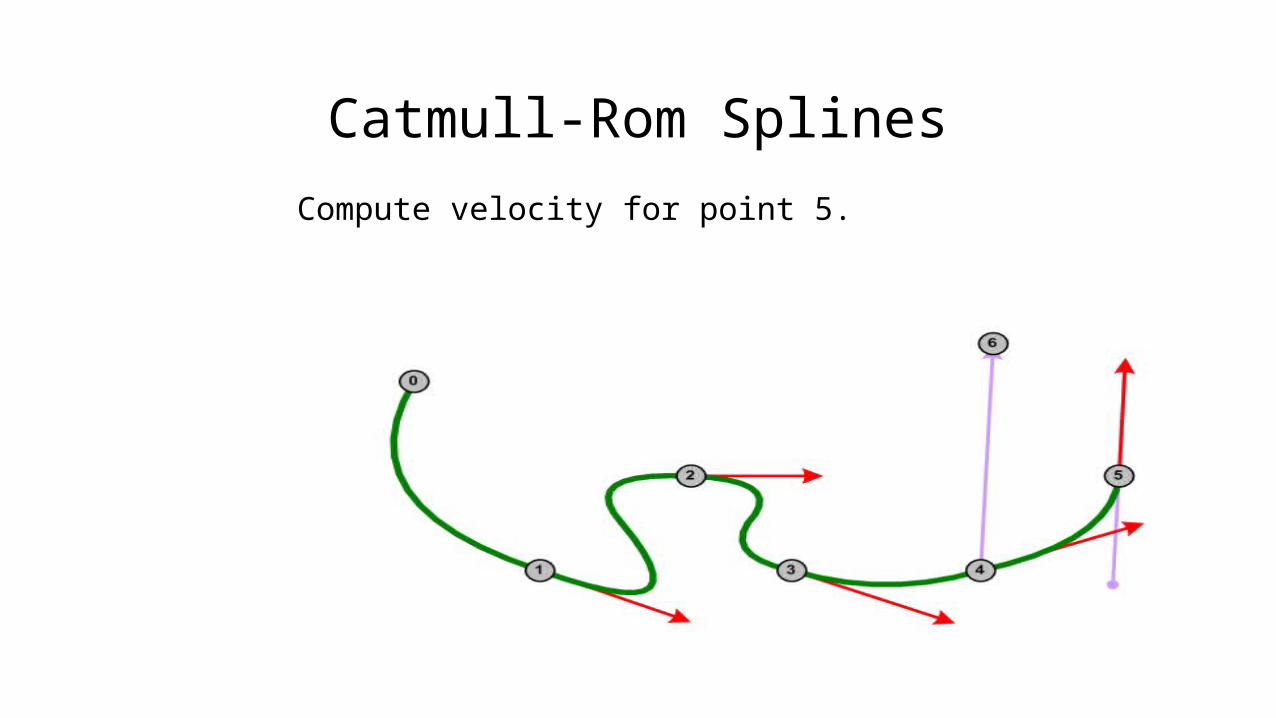
Catmull-Rom Splines
Compute velocity for point 5.
Catmull-Rom Splines
We already set the velocity for point 6 to be zero, so we can close out the spline.
Catmull-Rom Splines
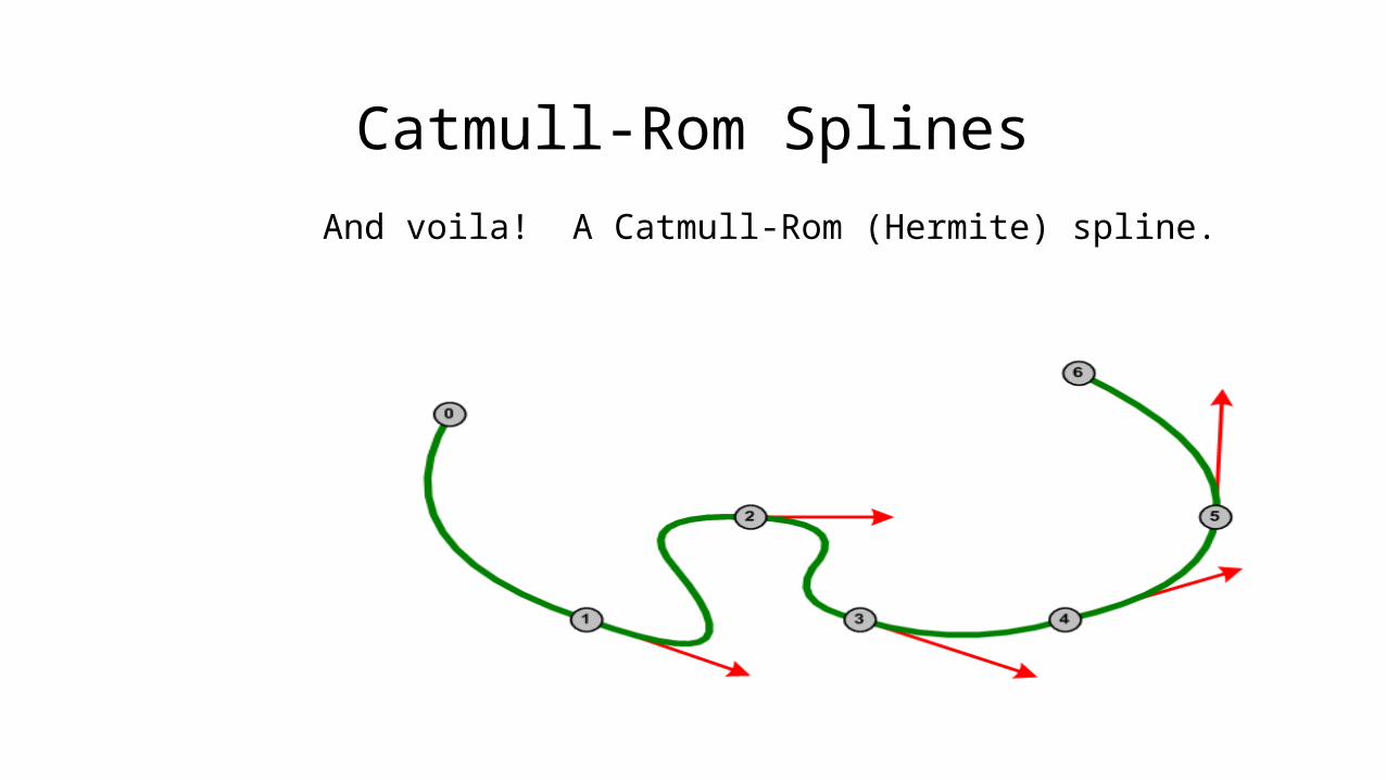
And voila! A Catmull-Rom (Hermite) spline.
Catmull-Rom Splines
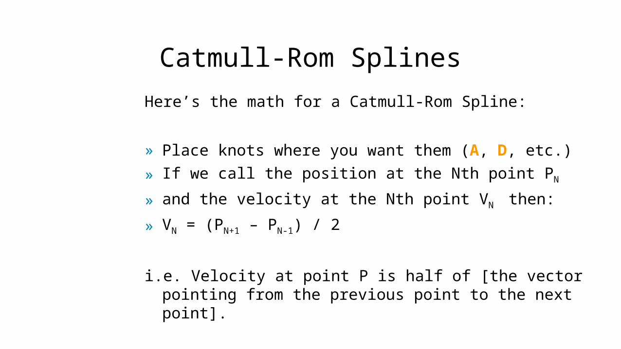
Here’s the math for a Catmull-Rom Spline:
» Place knots where you want them (A, D, etc.)
» If we call the position at the Nth point PN
» and the velocity at the Nth point VN then:
» VN = (PN+1 – PN-1) / 2
i.e. Velocity at point P is half of [the vector pointing from the previous point to the next point].

Cardinal Splines
Cardinal Splines
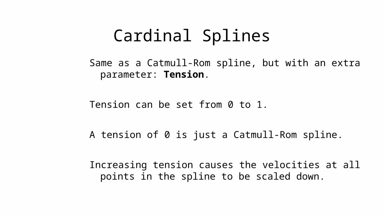
Same as a Catmull-Rom spline, but with an extra parameter: Tension.
Tension can be set from 0 to 1.
A tension of 0 is just a Catmull-Rom spline.
Increasing tension causes the velocities at all points in the spline to be scaled down.
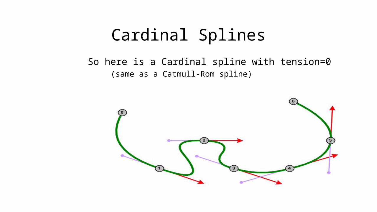
Cardinal Splines
So here is a Cardinal spline with tension=0(same as a Catmull-Rom spline)

Cardinal Splines
So here is a Cardinal spline with tension=.5(velocities at points are ½ of the Catmull-Rom)
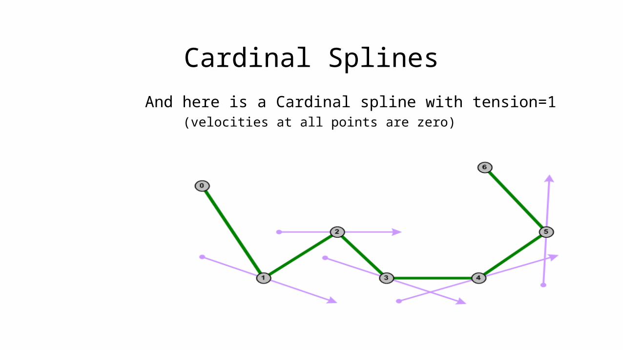
Cardinal Splines
And here is a Cardinal spline with tension=1(velocities at all points are zero)
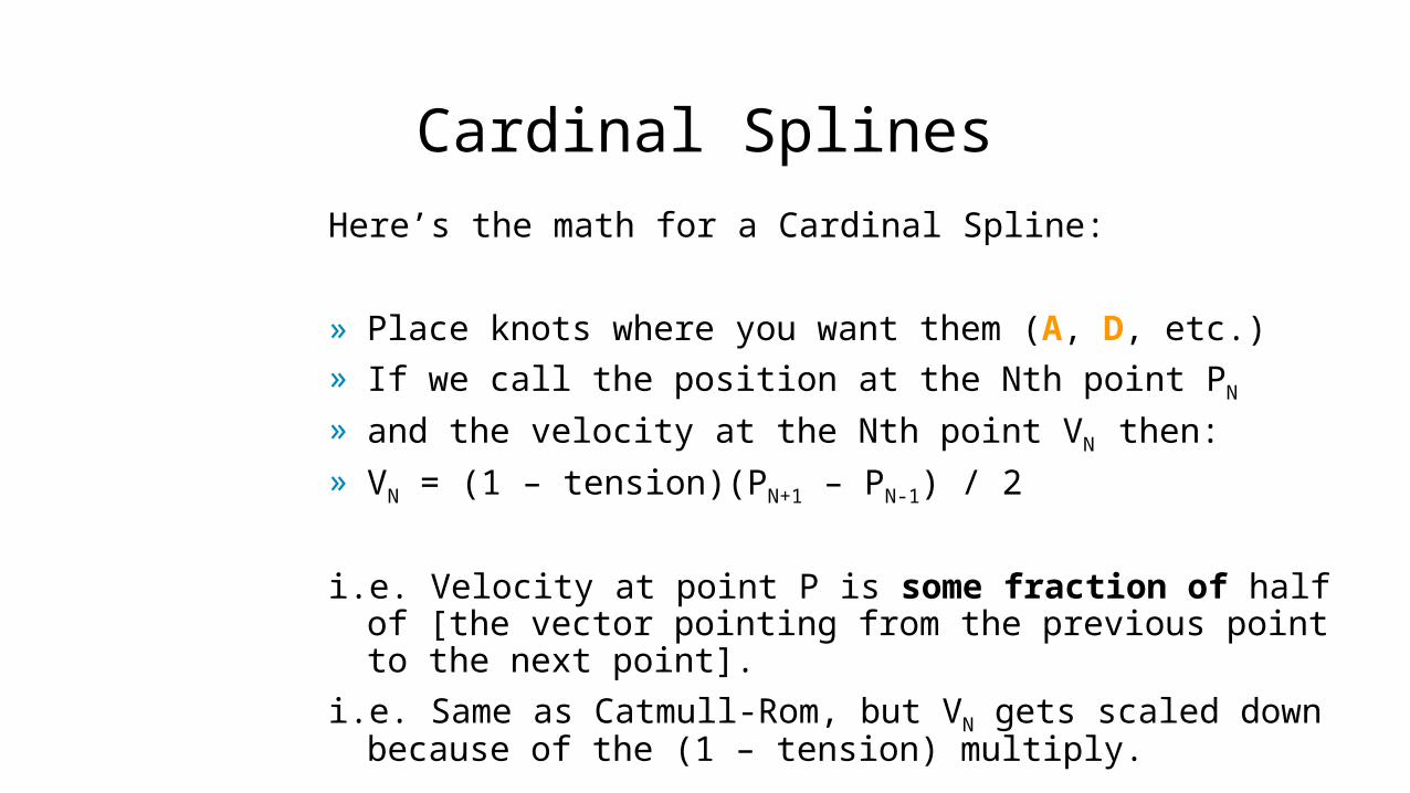
Cardinal SplinesHere’s the math for a Cardinal Spline:
» Place knots where you want them (A, D, etc.)» If we call the position at the Nth point PN
» and the velocity at the Nth point VN then:» VN = (1 – tension)(PN+1 – PN-1) / 2
i.e. Velocity at point P is some fraction of half of [the vector pointing from the previous point to the next point].
i.e. Same as Catmull-Rom, but VN gets scaled down because of the (1 – tension) multiply.

Other Spline Types
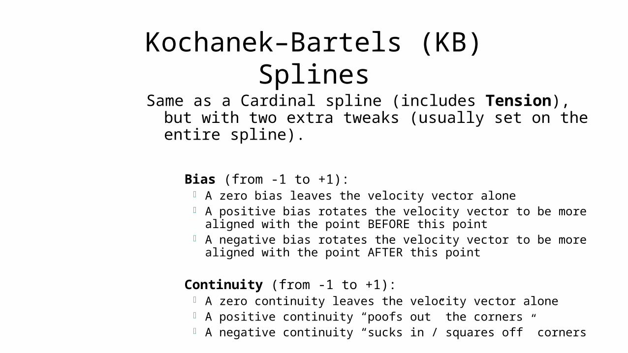
Kochanek–Bartels (KB) SplinesSame as a Cardinal spline (includes Tension), but with
two extra tweaks (usually set on the entire spline).
Bias (from -1 to +1): A zero bias leaves the velocity vector alone A positive bias rotates the velocity vector to be more aligned with
the point BEFORE this point A negative bias rotates the velocity vector to be more aligned with
the point AFTER this point
Continuity (from -1 to +1): A zero continuity leaves the velocity vector alone A positive continuity “poofs out” the corners A negative continuity “sucks in / squares off” corners
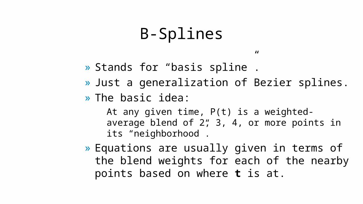
B-Splines
» Stands for “basis spline”.» Just a generalization of Bezier splines.» The basic idea:
At any given time, P(t) is a weighted-average blend of 2, 3, 4, or more points in its “neighborhood”.
» Equations are usually given in terms of the blend weights for each of the nearby points based on where t is at.

Splines as filtering/easing functions
Note: You can also use 1-dimensional splines (x only) as a way to “mess with” any value t (especially if t is a parametric value from 0 to 1), thereby making “easing” or “filtering” functions.
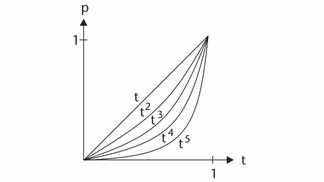
Some examples:» A simple “smooth start” function (such as t2) is really just
a quadratic Bezier curve where B is “on top of” A.» A simple “smooth stop” function (such as 2t – t2) is just a
quadratic Bezier curve where B is “on top of” C.» A simple “smooth start and stop” function (such as 3t2 –
2t3) is just a cubic Bezier curve where B=A and C=D.

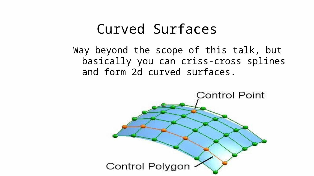
Curved Surfaces
Way beyond the scope of this talk, but basically you can criss-cross splines and form 2d curved surfaces.
Top Related