


Languages
Pages
Legal

Accepted for publication in Artificial Intelligence in Medicine. Draft v20.1, March 18, 2016.
1
From complex questionnaire and interviewing data
to intelligent Bayesian Network models for medical
decision support
Anthony Costa Constantinoua, c, Norman Fentona, William Marsha, and Lukasz Radlinskib
a) Risk and Information Management Research Group, School of Electronic Engineering and
Computer Science, Queen Mary University of London, Mile End Road, Mile End Campus,
Computer Science Building, E1 4NS, London, UK.
b) Department of Software Engineering, West Pomeranian University of Technology, Szczecin
ul. Żołnierska 52, 71-210 Szczecin, Poland
c) Corresponding author. E-mail address: [email protected]
THIS IS A PRE-PUBLICATION DRAFT OF THE FOLLOWING CITATION:
Constantinou, A. C., Fenton, N., Marsh, W., & Radlinski, L. (2016). From complex questionnaire and
interviewing data to intelligent Bayesian Network models for medical decision support. Artificial
Intelligence in Medicine, 67: 75-93.
DOI: 10.1016/j.artmed.2016.01.002
Corresponding author: Dr. Anthony Constantinou, E-mail: [email protected]
© 2016. This manuscript version is made available under the CC-BY-NC-ND 4.0 license:
http://creativecommons.org/licenses/by-nc-nd/4.0/
Accepted for publication in Artificial Intelligence in Medicine. Draft v20.1, March 18, 2016.
2
Abstract
Objectives: 1) To develop a rigorous and repeatable method for building effective Bayesian network
(BN) models for medical decision support from complex, unstructured and incomplete patient
questionnaires and interviews that inevitably contain examples of repetitive, redundant and
contradictory responses; 2) To exploit expert knowledge in the BN development since further data
acquisition is usually not possible; 3) To ensure the BN model can be used for interventional analysis;
4) To demonstrate why using data alone to learn the model structure and parameters is often
unsatisfactory even when extensive data is available.
Method: The method is based on applying a range of recent BN developments targeted at helping
experts build BNs given limited data. While most of the components of the method are based on
established work, its novelty is that it provides a rigorous consolidated and generalised framework
that addresses the whole life-cycle of BN model development. The method is based on two original
and recent validated BN models in forensic psychiatry, known as DSVM-MSS and DSVM-P.
Results: When employed with the same datasets, the DSVM-MSS demonstrated competitive to
superior predictive performance (AUC scores 0.708 and 0.797) against the state-of-the-art (AUC scores
ranging from 0.527 to 0.705), and the DSVM-P demonstrated superior predictive performance (cross-
validated AUC score of 0.78) against the state-of-the-art (AUC scores ranging from 0.665 to 0.717).
More importantly, the resulting models go beyond improving predictive accuracy and into usefulness
for risk management purposes through intervention, and enhanced decision support in terms of
answering complex clinical questions that are based on unobserved evidence.
Conclusions: This development process is applicable to any application domain which involves large-
scale decision analysis based on such complex information, rather than based on data with hard facts,
and in conjunction with the incorporation of expert knowledge for decision support via intervention.
The novelty extends to challenging the decision scientists to reason about building models based on
what information is really required for inference, rather than based on what data is available and
hence, forces decision scientists to use available data in a much smarter way.
Keywords: decision support, expert knowledge, Bayesian networks, belief networks, causal
intervention, questionnaire data, survey data, mental health, criminology, forensic psychiatry.
Accepted for publication in Artificial Intelligence in Medicine. Draft v20.1, March 18, 2016.
3
1 Introduction
Bayesian networks (BNs) are a well-established graphical
formalism for encoding the conditional probabilistic
relationships among uncertain variables of interest. The
nodes of a BN represent variables and the arcs between
variables represent causal, influential, or correlated
relationships. The structure and the relationships in BNs
can rely on both expert knowledge and relevant
statistical data, meaning that they are well suited for
enhanced decision making.
Underpinning BNs is Bayesian probability
inference that provides a way for rational real-world
reasoning. Any belief about uncertainty of some event A
is assumed to be provisional upon experience or data
gained to date. This is what we call the prior probability,
written P(A). This prior probability is then updated by
new experience or data B to provide a revised belief
about the uncertainty of A that we call the posterior
probability, written P(A|B). The term Bayesian comes
from Bayes' theorem which is a formula to determine
P(A|B):
𝑃(𝐴|𝐵) = 𝑃(𝐵|𝐴) × 𝑃(𝐴)
𝑃(𝐴)
Most real-world problems, including typically,
medical risk assessment problems, involve multiple
related uncertain variables and data, which are ideally
represented as BNs. Early attempts to use Bayesian
analysis in Artificial Intelligence applications to medical
problems were unsuccessful due to the necessary
Bayesian inference being, in general, computationally
intractable [1]. However, the development of efficient BN
inference propagation algorithms that work for large
classes of practical BNs [2-4], along with advances in
computational power over the last couple of decades, has
caused a renewed interest in Bayesian probability for
decision support. This has led to an enormous number of
BN applications in a wide range of real-world problems
[5] including, of course, medicine [6-9]. BNs are now
being recognised as a powerful tool for risk analysis and
decision support in real-world problems.
However, despite their demonstrable benefits,
BNs still remain under-exploited, partly because there
are no proven repeatable methods for their development
when the development process requires the
incorporation of expert knowledge due to limited or
inappropriate data for inference. The problem is
especially challenging when the only data available
comes from poorly structured questionnaires and
interviews involving answers to hundreds of relevant
questions, but including inevitably examples of
repetitive, redundant and contradictory responses. This
is what we define as 'complex' data.
The objective of this paper is to propose a
generic, repeatable, method for developing BNs by
exploiting expert judgment and typically complex data
that is common in medical problems. The method is
specifically targeted to deal with the extremely common
scenario, whereby the existing data cannot be extended
except for the incorporation of expert knowledge. So
there is no possibility of requesting data for either
additional samples or additional variables. Essentially,
we have to make the most of what we are given.
The method is derived from two case studies
from the domain of forensic psychiatry. Specifically:
1. DSVM-P (”Decision Support Violence Management –
Prisoners”): a BN model for risk assessment and risk
management of violent reoffending in released
prisoners, many of whom suffer from mental health
problems with serious background of violence [10];
2. DSVM-MSS (”Decision Support Violence Management -
Medium Security Services”): a BN model for violence
risk analysis in patients discharged from medium
security services [11].
Previously established predictive models in this
area of research are either regression based or rule-based
predictors, but their performance is poor and more
importantly, they are incapable of simulating complex
medical reasoning under uncertainty [10]. Hence, it was
felt that BN models could improve on the state-of-the-art.
The two BN models were developed in
collaboration with domain experts and the designers of
the questionnaires. Both models demonstrated improved
forecasting capability and enhanced usefulness for
decision support (as we demonstrate in Section 9 and
discuss in Sections 10 and 11) relative to the previous
state-of-the-art models in this area of research.
However, in both cases we had to overcome the
challenge of relying on patient data that had been
collected before the use of BNs had been considered. As
is typical with medical domain data much of it was
’complex’, in the sense described above, coming from
questionnaires and interviews with patients. The method
described in this paper for developing BN models based
on such existing complex data is an attempt to generalise
what we did and learned in these forensic psychiatry
applications.
While most of the components of the method are
based on established work, its novelty is as follows:
Accepted for publication in Artificial Intelligence in Medicine. Draft v20.1, March 18, 2016.
4
1. Provides a rigorous consolidated and generalised
framework that addresses the whole life-cycle of BN
model development for any application domain
where there is constrained and complex data.
Specifically where the problem involves decision
analysis based on complex information retrieved
from questionnaire and interview data, rather than
based on data with hard facts, and in conjunction
with the incorporation of expert knowledge.
2. Its starting point is an approach to problem framing
that challenges decision scientists to reason about
building models based on what information is really
required for inference, rather than based on what
data is available – even while it is assumed no new
data can be provided. In other words, it forces
decision scientists to use available data in a much
smarter way.
The questionnaire and interviewing data, and the
problems with learning from them, are discussed in
Section 2 along with relevant literature review and a brief
overview of the proposed method. Sections 3 to 8
describe the following respective steps of the method:
Determine model objectives, Bayesian Network structure, Data
Management, Parameter Learning, Interventional Modelling,
and Structural Validation. Drawing on the case study
results demonstrated in Section 9, we discuss the benefits
and limitations of the method in Section 10, we provide a
general discussion about the method and future research
in Section 11, and we provide our concluding remarks in
Section 12.
2 The data and its problems
As is typical for most medical BN building projects, in
the forensic psychiatry studies we were presented with a
set of unstructured patient data from questionnaires and
interviews that had been collected independently of the
requirements of a BN model. The questionnaires were
large and complex and the data extracted from them was
combined with other relevant patient data, such as
criminal records, retrieved by the Police National
Computer.
The questionnaire data includes patient
responses to questions over the course of an interview
with a specialist. They also include assessment data
based on certain check-lists formulated by specialists,
and which are taken into consideration for evaluating
certain psychological and psychiatric aspects of the
individual under assessment. The responses can take any
form, from binary scale (such as Yes/No) and ordinal
scale (such as Very low to Very high), to highly
complicated multiple choice answers (with one or more
possible selections), numerical answers (e.g. salary,
number of friends), as well as free-from answers.
For example, in the DSVM-P study individuals
were asked to complete up to 939 questions. All of the
responses are coded in a database, and each response is
represented by a variable. Since many of those questions
were based on multiple choice answers (with up to
approximately 20 choices), and with more than one
answer being selected in most of the cases, the resulting
database included a number of responses that was a
multiple of the number of questions. As a result, there
were thousands of variables in the relevant databases,
excluding the data from criminal records retrieved by the
Police National Computer. In the DSVM-MSS study,
which was based on less extensive questionnaires, the
total number of data variables was still well over 1,000.
Yet, despite the large number of variables, the
databases in both studies had relatively small sample
sizes (953 and 386 samples respectively for DSVM-P and
DSVM-MSS) - again something that is very typical of
many such studies. This makes them a poor starting
point for developing effective BNs for decision-support
and risk assessment, which normally require a very high
ratio of samples to variables and/or substantial expert
knowledge. This point is increasingly widely
understood; we do not restrict the complexity of the
model simply because we have limited or poor quality
data [12, 13]. BN applications which incorporate expert
knowledge along with relevant statistical data have
demonstrated significant improvements over models that
rely only on what data is available; specifically in real-
world applications requiring decision support [5, 14-18].
There have been limited previous attempts to
develop BN models from questionnaire, interviewing or
survey data:
1. Blodgett and Anderson [19] developed a BN model
to analyse consumer complaints and concluded that
the Bayesian framework offered rich and descriptive
overview of the broader complaining behaviour
process by providing insights into the determinants
and subsequent behavioural outcomes, such as
negative and positive word-of-mouth behaviour.
2. Sebastiani and Ramoni [20] developed a BN to
analyse a dataset extracted from the British general
household survey. The authors commented on the
limitation of having to discretise all the data since
continuous distributions were not supported by BN
software at that time.

Accepted for publication in Artificial Intelligence in Medicine. Draft v20.1, March 18, 2016.
5
3. Ronald et al. [21] found the following advantages of
BNs (compared to more traditional statistical
techniques) in analysing key linkages of the service-
profit chain within the context of transportation
service satisfaction: a) can provide causal explanation
using observable variables within a single
multivariate model, b) analyse nonlinear
relationships contained in ordinal measurements, c)
accommodate branching patterns that occur in data
collection, and d) provide the ability to conduct
probabilistic inference for prediction and diagnostics
with an output metric that can be understood by
managers and academics.
4. Salini and Kenett [22] examined BNs in analysing
customer satisfaction from survey data with the
intention of demonstrating the advantages of BNs in
dealing with this type of data on the basis that "BNs
have been rarely used so far in analyzing customer
satisfaction data" [22].
5. Ishino [23] described a method of extracting
knowledge from questionnaires for marketing
purposes by performing BN modelling. This method
was said to be a) capable of treating multiple
objective variables in one model, b) handling
nonlinear covariation between variables, and c)
solving feature selection problems using Cramer's
coefficient of association as an indicator [23]; though
the benefits of (1) and (2) come as a result of using
the BN framework.
With the exception of Ishino [23] the main focus
of these previous studies were on the results and benefits
of the developed BNs, rather than on the method of
development. Moreover, all applications involved data
from surveys and questionnaires for marketing and
customer satisfaction purposes - generally a less complex
application domain than medical. While Ishino [23], did
focus on a method, it involved minimal expert input. Our
focus is on a method for moving from the poorly
structured, complex, but limited, data to an effective
expert constructed BN model. Hence, we believe this is
the first attempt to provide a whole-life cycle process for
developing and validating BN models based on complex
data and expert judgment.
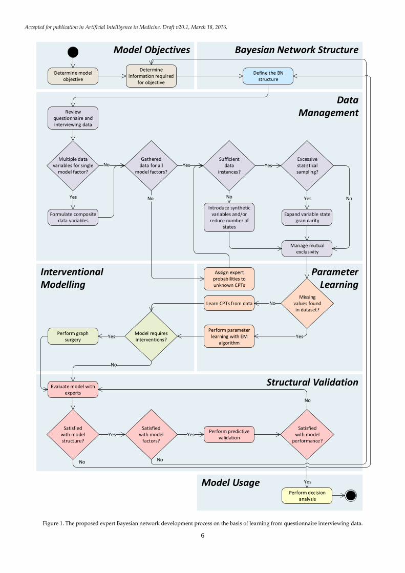
The method is divided into six key component
steps, as demonstrated by the iterative development
process in Figure 1.
The following sections, from Section 3 to Section
8, describe respectively the six steps. Throughout, we
illustrate each step with examples from the two case
studies and discuss the challenges for each development
step in detail.
Accepted for publication in Artificial Intelligence in Medicine. Draft v20.1, March 18, 2016.
6
Model Objectives
Model Usage
Bayesian Network Structure
Structural Validation
InterventionalModelling
ParameterLearning
DataManagement
Determine model objective
Determine information required
for objective
Define the BN structure
Review questionnaire and interviewing data
Formulate composite data variables
Multiple datavariables for single
model factor?
Gathereddata for all
model factors?
Assign expert probabilities to unknown CPTs
Sufficientdata
instances?
Excessivestatisticalsampling?
Expand variable state granularity
Introduce synthetic variables and/or
reduce number of states
Manage mutual exclusivity
Missingvalues foundin dataset?
Learn CPTs from data
Perform parameter learning with EM
algorithm
Model requires interventions?
Perform graph surgery
Evaluate model with experts
Satisfiedwith model
performance?
Satisfiedwith modelstructure?
Satisfiedwith model
factors?
Perform predictive validation
Perform decision analysis
Yes No
No Yes Yes
No Yes
Yes
No
Yes
No
Yes Yes
Yes
No
No No
No
Figure 1. The proposed expert Bayesian network development process on the basis of learning from questionnaire interviewing data.

Accepted for publication in Artificial Intelligence in Medicine. Draft v20.1, March 18, 2016.
7
3 Model objectives
The starting point of the method is the Model
Objectives component. Although the availability of some
existing patient/medical database is often the motivation
to develop a BN (“we have this really great/important data –
we think you should be able to use it to build a BN model to
support decision making for problem X…”) it should never
be the real starting point. This is true even in the scenario
(which is the one we are assuming) whereby the
available data cannot be extended except by expert
knowledge. Instead, irrespective of whatever existing
data is available (and certainly before even considering
doing any kind of statistical analysis) the first step
involves determining what the actual objective of the
model is. For example, the following are very different
classes of objectives for BN models:
1. Risk assessment: Determine the most likely current
state of a variable (that is typically not directly
observable). For example, “to determine from all the
available information, the probability that a given person
has disease X” or “to determine if new drug D is safe to
use”.
2. Risk Management: Determine the most likely outcome
of some core variable for a given intervention action.
For example, “What is the probability a patient’s
condition with respect to disease X will improve if given
treatment T”.
In the DSVM-P study the initial core objective
was to determine if it is safe to release a given prisoner
by assessing the prisoner's risk of violent reoffending in
the case of release. Similarly, the core objective for the
DSVM-MSS study was to determine if it is safe to
discharge a given mentally ill patient by assessing the
patient's risk of violence in the case of discharge. Both of
these objectives represent a risk assessment process. But in
both case studies, the objectives are expanded to risk
management in the sense that the risk of violence for a
given individual can be managed to acceptable levels
after release/discharge by considering a number of
relevant interventions (see Section 7).
Only when the objective is determined, can we
specify what information we ideally require for carrying it
out. Interviews with one or more domain experts are
typically required in order to identify all of the important
variables required to meet the core objective for the BN
model. For our two BN applications, the domain experts
were two clinical active experts in forensic psychiatry
(Prof. Jeremy Coid) and forensic psychology (Dr. Mark
Freestone) [10, 11]. In each case approximately five to
seven meetings lasting between 1-2 hours with the
domain experts were required at this stage in order to
identify the important model factors (this really depends
on domain complexity). In both studies, at least 75% of
the model factors were identified at this initial stage.
The subsequent component of our proposed
method is concerned with constructing a Bayesian
network structure, in collaboration with domain experts,
by considering the information that we really need to
model.
4 Bayesian network structure
Assuming we have specified the 'ideal' required
variables from the model objectives step, we can proceed
into the most time consuming step of the process:
constructing the structure of the BN model with expert
knowledge. While BNs are often used to represent causal
relationships between variables of interest, an arc from
variable A to variable B does not necessarily require that
B is causally dependent on A [13]. The 'ideal' variables
constitute the initial set of nodes of the BN. Many BNs
developed for medical real-world applications have been
constructed by expert elicitation [6, 9, 24-28].
We do recognise that expert elicitation requires
major interdisciplinary collaboration which can be
complex and time consuming. In the DSVM-P study 75%
of the model factors had been identified as a result of
investigating what information we really require to meet
the model objectives. It is only when the experts are
involved in the design of the BN structure, and therefore
start thinking in terms of dependency and/or cause and
effect between factors, that they are able to identify the
residual factors that were missed in the previous step.
Unlike the previous step, however, in the BN
structure step the meetings were numerous and long. In
DSVM-P there were around 20 meetings whose average
time was approximately three hours. However, since we
collaborated with the same experts for both case studies,
the development of the BN structure for the second case
study DSVM-MSS was approximately three to four times
shorter than that of DSVM-P. We believe there were two
reasons for this: 1) the experts had already ‘learned’
about both the process and BN models; and 2) there were
generic similarities between the second and first study. As noted in Figure 1, the BN structure we
initially construct is likely to be quite different from the
final version (as a result of subsequent iterations to
model synthetic and mutually exclusive variables and
also interventions). However, the conceptual flow of the
network is likely to remain unchanged. Figures 2, 5 and 8
from respective Sections 5.2, 5.4 and 7 demonstrate how
Accepted for publication in Artificial Intelligence in Medicine. Draft v20.1, March 18, 2016.
8
fragments of the BN model have been altered over the
process as a result of introducing synthetic, mutual
exclusive and interventional nodes in the BNs. The final
versions of the two BNs are provided in Appendix A;
Figures A1 and A2. The next component of our proposed
method is concerned with mapping the data we actually
have into the closest possible match to what we ideally
need.
5 Data management
The primary objective of the data management task is to
link actual data variables to model nodes. Because of the
complexity of the data from questionnaires and
interviews as described in Section 2, this is extremely
challenging. Generally, there is no single data variable
corresponding to an ideal' model variable. Typically
there are multiple related data variables provided for
similar questions. The challenge here mainly involves
combining all these similar responses (which in some
cases can also be inconsistent) into a single piece of
information in an attempt to inform the relevant model
node. These challenges are discussed in the following
sub-subsections.
5.1. Composite data variables
The most common problem involves the need for a single
variable which, although not in the data, has multiple
associated variables. For example, in the DSVM-P study
we had the following model nodes:
1. Financial difficulties: While there was no such variable
in the available questionnaire data there was
sufficient information to learn an approximate
surrogate variable. Specifically, the sources of such
relevant information are answers provided to
questions such as "Are you behind paying bills?",
"Have you recently had any services cut off?", and "What
is your average weekly income".
2. Problematic life events: This was assessed on the basis
of responses to questions such as "Separation due to
marital difficulties, divorce or break down of steady
relationship", "Serious problem with a close friend,
neighbour or relative", and "Being made redundant or
sacked from your job".
For both of these examples there were several
more relevant sources of information that could have
been considered to learn the specific model variables,
and this was the case with many other model factors. As
a result, problems arise in determining which data
variable to choose for the particular node. Focusing on
just one data variable is not expected to be the best
approach since, in doing so, other relevant and important
information will most likely be ignored.
A solution under these expert-driven
circumstances is to formulate some combinational rule,
or a set of combinational rules, for all the important data
variables. We have worked with clinicians (psychiatrists
and clinical psychologists) as well as the designers of the
questionnaires themselves to retrieve the inferences we
were interested in [10, 11]. Examples of combinational
rules between the different sources of similar information
are:
1. an OR relationship - i.e. Financial difficulties="Yes" if at
least one data variable satisfies this statement,
2. an AND relationship - i.e. Financial difficulties="Yes" if
all the relevant data variables satisfy this statement,
3. a relative counter - i.e. Financial difficulties="Yes" if at
least X out of Y data variables satisfy this statement,
4. a ranked average - i.e. Financial difficulties="Very high"
if the majority of the data variables indicate severe
financial difficulties,
5. a weighted ranked average - i.e. Financial
difficulties="Very high" if the key data variables
indicate severe financial difficulties.
Although many other combinational rules are possible,
the five above should be enough to deal with the vast
majority of these scenarios.
One class of cases, however, is especially
problematic, namely where the data actually comprises
records of expert knowledge. For instance, some records
may reflect the clinician’s assessment as to whether the
individual suffers from a particular type of mental
illness, or in identifying a certain type of behavioural
attitude by interviewing the individual. In such
situations we found it impractical to derive a clear-cut
method of determining which combinational rules to use
and when because the questionnaire and interviewing
data was far too complex and uncertain. As a result, in
these situations we required expert judgements to
determine the necessary data sources and combinational
rules.
Accepted for publication in Artificial Intelligence in Medicine. Draft v20.1, March 18, 2016.
9
5.2. Synthetic BN nodes
Although many relations in a BN can be causal, one of
the most commonly occurring class of BN fragments is
not causal at all. The definitional/synthesis idiom models
this class of BN fragments.
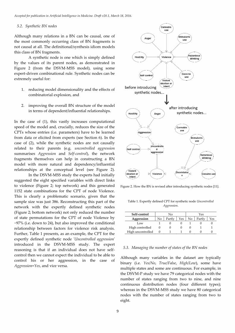
A synthetic node is one which is simply defined
by the values of its parent nodes, as demonstrated in
Figure 2 (from the DSVM-MSS model), using some
expert-driven combinational rule. Synthetic nodes can be
extremely useful for:
1. reducing model dimensionality and the effects of
combinatorial explosion, and
2. improving the overall BN structure of the model
in terms of dependent/influential relationships.
In the case of (1), this vastly increases computational
speed of the model and, crucially, reduces the size of the
CPTs whose entries (i.e. parameters) have to be learned
from data or elicited from experts (see Section 6). In the
case of (2), while the synthetic nodes are not causally
related to their parents (e.g. uncontrolled aggression
summarises Aggression and Self-control), the network
fragments themselves can help in constructing a BN
model with more natural and dependency/influential
relationships at the conceptual level (see Figure 2).
In the DSVM-MSS study the experts had initially
suggested the eight specified variables with direct links
to violence (Figure 2; top network) and this generated
1152 state combinations for the CPT of node Violence.
This is clearly a problematic scenario, given that the
sample size was just 386. Reconstructing this part of the
network with the expertly defined synthetic nodes
(Figure 2; bottom network) not only reduced the number
of state permutations for the CPT of node Violence by
~97% (i.e. down to 24), but also improved the conditional
relationship between factors for violence risk analysis.
Further, Table 1 presents, as an example, the CPT for the
expertly defined synthetic node 'Uncontrolled aggression'
introduced in the DSVM-MSS study. The expert
reasoning is that if an individual does not have self-
control then we cannot expect the individual to be able to
control his or her aggression, in the case of
Aggression=Yes, and vice versa.
Figure 2. How the BN is revised after introducing synthetic nodes [11].
Table 1. Expertly defined CPT for synthetic node Uncontrolled
Aggression.
Self-control No Yes
Aggression No Partly Yes No Partly Yes
Low 1 0 0 1 0 0
High controlled 0 0 0 0 1 1
High uncontrolled 0 1 1 0 0 0
5.3. Managing the number of states of the BN nodes
Although many variables in the dataset are typically
binary (i.e. Yes/No, True/False, High/Low), some have
multiple states and some are continuous. For example, in
the DSVM-P study we have 79 categorical nodes with the
number of states ranging from two to nine, and nine
continuous distribution nodes (four different types);
whereas in the DSVM-MSS study we have 80 categorical
nodes with the number of states ranging from two to
eight.

Accepted for publication in Artificial Intelligence in Medicine. Draft v20.1, March 18, 2016.
10
If we are learning the prior probabilities of the
states from the data alone we need to ensure there not
too many states relative to the sample size. If there are
the learned probabilities will suffer from high variability,
which typically results in model overfitting; i.e. leading to
a model that performs well on the training data but
poorly on unseen data. This happens when the model
has not learned to generalise from trend. Depending on
the parent nodes, sometimes even three states will be too
many, while some variables may have up to 10+ states.
Under such circumstances, some sensible re-
categorisation of states must be performed in order to
reduce the number of states for such variables.
Figure 3 illustrates a case from the DSVM-P
study whereby we had to convert a Gaussian distribution
of IQ scores into a categorical distribution consisting of
six ordinal states. A quick look at the prior marginal
probabilities of the categorical distribution, which appear
to be normally distributed over the six states, as captured
from data, provides us with confidence the size of data
was sufficient for a reasonably well informed prior.
Conversely, for the DSVM-MSS study the limited data
restricted the number of states of the IQ node to just
three. Appendix B, Table B.1 provides all the variables,
from both models that have been downgraded in terms
complexity in order to reduce the risk of model overfitting
as a result of limited data.
Figure 3. Converting a Gaussian distribution into a categorical
distribution, as captured from data, with ordinal states. Note that the
average IQ of the individuals in the study was below average.
When the states of the variable are known to
follow an ordinal scale distribution, but the dataset is not
sufficiently large to capture the normality as accurate as
that of Figure 3, other approaches can be considered such
as Ranked nodes in BNs which are ordinal categorical
distributions generated on the basis of Truncated Gaussian
distributions [29]. Figure 4 demonstrates how the same
Gaussian distribution from Figure 3 can be converted into
a Ranked distribution of the same six states by
normalising the mean and variance into a truncated
version with lower and upper boundaries set to 0 and 1
respectively; effectively a TruncatedGaussian[0,1]
distribution as proposed by [29].
Figure 4. Converting a Gaussian distribution into a Ranked distribution
based on the mean and variance of the Gaussian distribution, as
proposed by Fenton et al. [29].
Properly managing the type of nodes (i.e.
categorical/continuous), the number of node states, and
the type of states (i.e. nominal/ordinal), can dramatically
help in increasing computational speed while
concurrently improving the model's predictive accuracy.
5.4. Mutual exclusivity
Datasets resulting from questionnaires and interviews
will likely incorporate multiple variables that are
mutually exclusive. Such variables can usually be more
simply modelled in a BN as the set of states of another
single generalised variable (by definition such states are
mutually exclusive).
Figure 5. Collapsing mutual exclusive data variables into a single
generalised node with mutual exclusive states.
An example of this common phenomena arising
in the DSVM-P study is shown in Figure 5. Here there is
a set of seven mutually exclusive Boolean variables in the
Accepted for publication in Artificial Intelligence in Medicine. Draft v20.1, March 18, 2016.
11
dataset (there were many more but the experts identified
these seven to be sufficient and the most important); they
can be collapsed into a single generalised categorical
node. This assumes that all of the mutual exclusive
variables share identical parent and child nodes, and are
therefore not required to be modelled as distinct nodes
[30]. Properly managing mutual exclusivity reduces
model complexity, makes parameter learning and
elicitation simpler, and increases computational speed.
6 Parameter learning
Parameter learning is the process of determining the CPT
entries for each node of the agreed BN model. It is
expected to be performed once the model structure is
stable and all of the data management issues have been
satisfactorily addressed
Because of the limitations of the real-world data,
even allowing for the methods described in Section 5,
there will generally be nodes or individual parameter
values, for which no relevant data is available. For these
cases, we chose to elicit the probability values from the
domain experts (in the DSVM-P study four out of 89 of
the nodes required expert elicitation, while in the
DSVM-MSS study it was six out of 80 such nodes). We
address this process in Section 6.1. Alternatively, there
are data-driven techniques which could be considered
for finding reasonable assignments to missing variables,
and this is covered in Section 6.2 where we describe the
method for learning the CPTs from data.
6.1. Expert-driven learning
Various expert-driven probability elicitation methods
have been proposed. However, most of them are similar
and rather simple as they tend to propose some sort of
probability scale with verbal and/or numerical anchors,
as well as focusing on speeding up the elicitation process
as it can sometimes be a daunting task [27, 31-33].
The expert-driven probability elicitation process
we considered for both case studies was similar to those
referred above, using verbal representations for
probability scale such as from Very low (i.e. 0 to 0.2) to
Very high (i.e. 0.8 to 1). We also endeavoured to keep the
questions put to experts as simple as possible; at no point
were the expert asked to combine multiple pieces of
uncertain information in their head in order to arrive at a
conclusion.
We ensured that domain experts would only be
required to answer straightforward questions such as:
"How strong is the influence between A and B?", or "how high
is the risk of treatment Y causing a side-effect?". We also
found helpful the following studies [5, 34-37] which, in
addition to providing further recommendations on
eliciting expert probabilities, also provide guidelines on
how to minimise bias during the elicitation process.
6.2. Data-driven learning
Unfortunately, in both our studies the vast majority of
the data-driven variables had missing data. The only
data-driven nodes with complete data were those based
on criminal data provided by the Police National
Computer (e.g. Age, Gender, Number of violent convictions).
This is typical of real-world data in medical domains
where it is generally accepted that patient data collected
during the course of clinical care will inevitably suffer
from missing data [38].
In dealing with datasets which include missing
data, decision scientists typically have three options [39]:
1. Restrict parameter learning only to cases with complete
data: For the reasons explained above this is not a
viable option for typical medical studies.
2. Use imputation-based approaches: In these missing
values are filled with the most probable value, based
on the values of known cases, and then the CPTs are
learned normally as if they were considering a full
dataset. There are multiple imputation methods; for
example, the imputed value can be chosen based on
the mean predicted value when considering all of the
other know values, or a subset of them, or even
based on regression procedures [40].
3. Use likelihood-based approaches: In these the missing
values are inferred from existing model and data (i.e.
the model attempts to infer the likelihood of missing
values that make the observed data most likely). The
Expected Maximisation (EM) algorithm, which is an
iterative method for approximating the values of
missing data [41], is commonly used for this
purpose, and is widely accepted as the standard
approach for dealing with missing data in BNs.
In both studies we chose option (3) and the EM
algorithm to learn the CPTs of variables which are based
on data with missing values. Specifically, the EM
algorithm is based on forming the conditional
expectation of the log-likelihood function for completed
data given the observed data as defined in [41]:
𝑄(𝜃′|𝜃) = 𝐸𝜃{𝑙𝑜𝑔 𝑓(𝑋|𝜃′)|𝑦},
Accepted for publication in Artificial Intelligence in Medicine. Draft v20.1, March 18, 2016.
12
where X is the random variable which corresponds to the
complete data, which is unobserved, with density f, and
𝑦 = 𝑔(𝑥) is the observed data. The log-likelihood
function for the complete data is a linear function of the
set of sufficient marginals:
𝑛(𝑖𝑎), 𝑎 Є 𝐴, 𝑖𝑎 Є 𝐼𝑎 .
The EM algorithm searches for the Maximum Likelihood
Estimate (MLE) of the marginal likelihood by iteratively
applying the following two steps:
1. Expectation (E) step. This calculates the expected
value of the log-likelihood function and which is
equivalent to calculating the expected marginal
counts:
𝑛∗(𝑖𝑎) = 𝐸𝑝{𝑁(𝑖𝑎)|observed data};
2. Maximisation (M) step. This solves:
𝑛(𝑖𝑎) = 𝑛∗(𝑖𝑎), 𝑎 Є 𝐴, 𝑖𝑎 Є 𝐼𝑎 ,
for p which, assuming the expected counts were
the true counts, maximises the likelihood
function.
For this task, we have made use of the EM learning
engine offered by the freely available GeNIe [42]. This is
because GeNIe offers the two following important
features during the learning process:
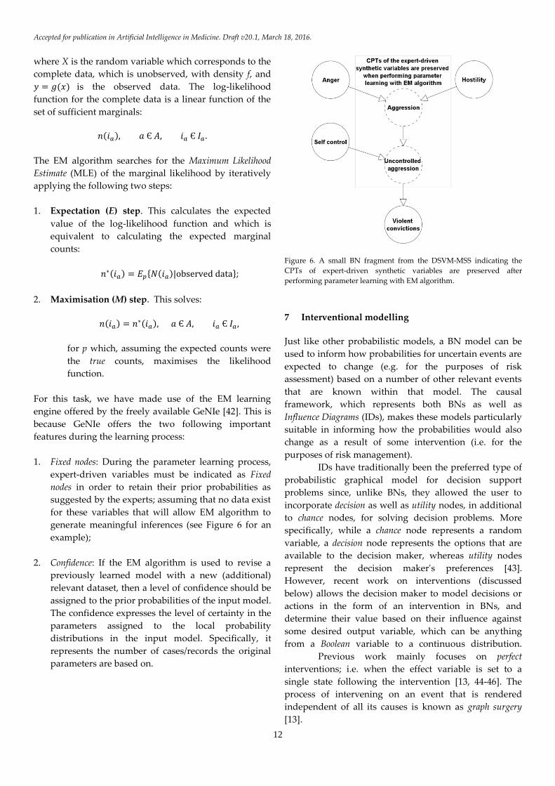
1. Fixed nodes: During the parameter learning process,
expert-driven variables must be indicated as Fixed
nodes in order to retain their prior probabilities as
suggested by the experts; assuming that no data exist
for these variables that will allow EM algorithm to
generate meaningful inferences (see Figure 6 for an
example);
2. Confidence: If the EM algorithm is used to revise a
previously learned model with a new (additional)
relevant dataset, then a level of confidence should be
assigned to the prior probabilities of the input model.
The confidence expresses the level of certainty in the
parameters assigned to the local probability
distributions in the input model. Specifically, it
represents the number of cases/records the original
parameters are based on.
Figure 6. A small BN fragment from the DSVM-MSS indicating the
CPTs of expert-driven synthetic variables are preserved after
performing parameter learning with EM algorithm.
7 Interventional modelling
Just like other probabilistic models, a BN model can be
used to inform how probabilities for uncertain events are
expected to change (e.g. for the purposes of risk
assessment) based on a number of other relevant events
that are known within that model. The causal
framework, which represents both BNs as well as
Influence Diagrams (IDs), makes these models particularly
suitable in informing how the probabilities would also
change as a result of some intervention (i.e. for the
purposes of risk management).
IDs have traditionally been the preferred type of
probabilistic graphical model for decision support
problems since, unlike BNs, they allowed the user to
incorporate decision as well as utility nodes, in additional
to chance nodes, for solving decision problems. More
specifically, while a chance node represents a random
variable, a decision node represents the options that are
available to the decision maker, whereas utility nodes
represent the decision maker's preferences [43].
However, recent work on interventions (discussed
below) allows the decision maker to model decisions or
actions in the form of an intervention in BNs, and
determine their value based on their influence against
some desired output variable, which can be anything
from a Boolean variable to a continuous distribution.
Previous work mainly focuses on perfect
interventions; i.e. when the effect variable is set to a
single state following the intervention [13, 44-46]. The
process of intervening on an event that is rendered
independent of all its causes is known as graph surgery
[13].
Accepted for publication in Artificial Intelligence in Medicine. Draft v20.1, March 18, 2016.
13
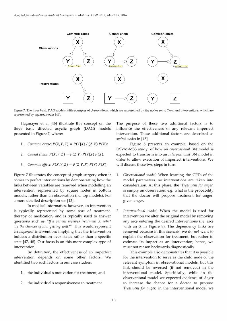
Figure 7. The three basic DAG models with examples of observations, which are represented by the nodes set to True, and interventions, which are
represented by squared nodes [46].
Hagmayer et al [46] illustrate this concept on the
three basic directed acyclic graph (DAG) models
presented in Figure 7, where:
1. Common cause: 𝑃(𝑋, 𝑌, 𝑍) = 𝑃(𝑌|𝑋) 𝑃(𝑍|𝑋) 𝑃(𝑋);
2. Causal chain: 𝑃(𝑋, 𝑌, 𝑍) = 𝑃(𝑍|𝑌) 𝑃(𝑌|𝑋) 𝑃(𝑋);
3. Common effect: 𝑃(𝑋, 𝑌, 𝑍) = 𝑃(𝑍|𝑌, 𝑋) 𝑃(𝑌) 𝑃(𝑋);
Figure 7 illustrates the concept of graph surgery when it
comes to perfect interventions by demonstrating how the
links between variables are removed when modelling an
intervention, represented by square nodes in bottom
models, rather than an observation (i.e. top models). For
a more detailed description see [13].
In medical informatics, however, an intervention
is typically represented by some sort of treatment,
therapy or medication, and is typically used to answer
questions such as: "If a patient receives treatment X, what
are the chances of him getting well?". This would represent
an imperfect intervention; implying that the intervention
induces a distribution over states rather than a specific
state [47, 48]. Our focus is on this more complex type of
intervention.
By definition, the effectiveness of an imperfect
intervention depends on some other factors. We
identified two such factors in our case studies:
1. the individual's motivation for treatment, and
2. the individual's responsiveness to treatment.
The purpose of these two additional factors is to
influence the effectiveness of any relevant imperfect
intervention. These additional factors are described as
switch nodes in [48].
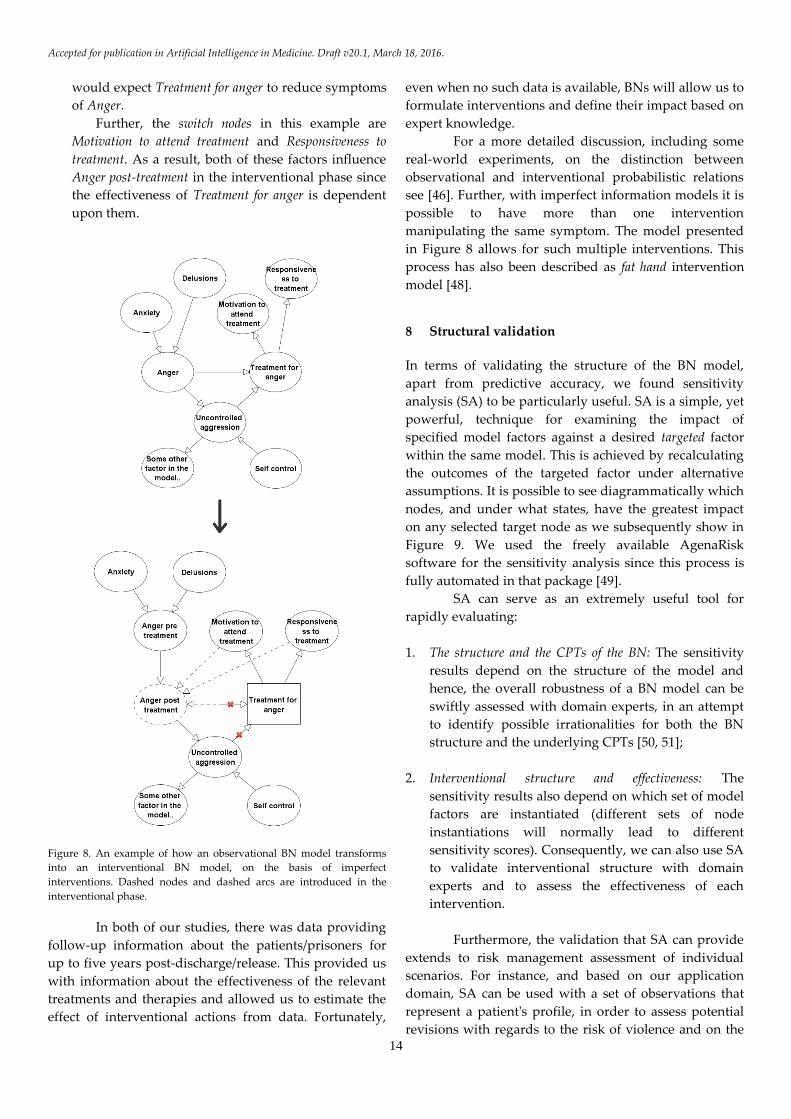
Figure 8 presents an example, based on the
DSVM-MSS study, of how an observational BN model is
expected to transform into an interventional BN model in
order to allow execution of imperfect interventions. We
will discuss these two steps in turn:
1. Observational model: When learning the CPTs of the
model parameters, no interventions are taken into
consideration. At this phase, the 'Treatment for anger'
is simply an observation; e.g. what is the probability
that the doctor will propose treatment for anger,
given anger.
2. Interventional model: When the model is used for
intervention we alter the original model by removing
any arcs entering the desired interventions (i.e. arcs
with an X in Figure 8). The dependency links are
removed because in this scenario we do not want to
explain the observation for treatment, but rather to
estimate its impact as an intervention; hence, we
must not reason backwards diagnostically.
This example also demonstrates that it is possible
for the intervention to serve as the child node of the
relevant symptom in observational models, but this
link should be reversed (if not removed) in the
interventional model. Specifically, while in the
observational model we expected evidence of Anger
to increase the chance for a doctor to propose
Treatment for anger, in the interventional model we
Accepted for publication in Artificial Intelligence in Medicine. Draft v20.1, March 18, 2016.
14
would expect Treatment for anger to reduce symptoms
of Anger.
Further, the switch nodes in this example are
Motivation to attend treatment and Responsiveness to
treatment. As a result, both of these factors influence
Anger post-treatment in the interventional phase since
the effectiveness of Treatment for anger is dependent
upon them.
Figure 8. An example of how an observational BN model transforms
into an interventional BN model, on the basis of imperfect
interventions. Dashed nodes and dashed arcs are introduced in the
interventional phase.
In both of our studies, there was data providing
follow-up information about the patients/prisoners for
up to five years post-discharge/release. This provided us
with information about the effectiveness of the relevant
treatments and therapies and allowed us to estimate the
effect of interventional actions from data. Fortunately,
even when no such data is available, BNs will allow us to
formulate interventions and define their impact based on
expert knowledge.
For a more detailed discussion, including some
real-world experiments, on the distinction between
observational and interventional probabilistic relations
see [46]. Further, with imperfect information models it is
possible to have more than one intervention
manipulating the same symptom. The model presented
in Figure 8 allows for such multiple interventions. This
process has also been described as fat hand intervention
model [48].
8 Structural validation
In terms of validating the structure of the BN model,
apart from predictive accuracy, we found sensitivity
analysis (SA) to be particularly useful. SA is a simple, yet
powerful, technique for examining the impact of
specified model factors against a desired targeted factor
within the same model. This is achieved by recalculating
the outcomes of the targeted factor under alternative
assumptions. It is possible to see diagrammatically which
nodes, and under what states, have the greatest impact
on any selected target node as we subsequently show in
Figure 9. We used the freely available AgenaRisk
software for the sensitivity analysis since this process is
fully automated in that package [49].
SA can serve as an extremely useful tool for
rapidly evaluating:
1. The structure and the CPTs of the BN: The sensitivity
results depend on the structure of the model and
hence, the overall robustness of a BN model can be
swiftly assessed with domain experts, in an attempt
to identify possible irrationalities for both the BN
structure and the underlying CPTs [50, 51];
2. Interventional structure and effectiveness: The
sensitivity results also depend on which set of model
factors are instantiated (different sets of node
instantiations will normally lead to different
sensitivity scores). Consequently, we can also use SA
to validate interventional structure with domain
experts and to assess the effectiveness of each
intervention.
Furthermore, the validation that SA can provide
extends to risk management assessment of individual
scenarios. For instance, and based on our application
domain, SA can be used with a set of observations that
represent a patient's profile, in order to assess potential
revisions with regards to the risk of violence and on the

Accepted for publication in Artificial Intelligence in Medicine. Draft v20.1, March 18, 2016.
15
basis of some intervention. As an example, Figure 9
presents the tornado graph 1 generated for risk
management purposes, based on a prisoner’s profile
from our case studies. The effectiveness of the three
specified interventions is assessed against the prisoner's
profile, and which indicates that the individual:
1. suffers from mental illness,
2. is drug dependent,
3. is alcohol dependent,
4. is partly impulsive,
5. has no violent thoughts,
6. is motivated to attend treatments,
7. is responsive to treatments and therapies
For instance, the graph indicates that if we set Psychiatric
treatment (P) to "No", we get p(Violence=Yes)=0.661,
whereas if we enable this particular intervention the
respective risk of violence drops down to 0.5342.
Figure 9. Sensitivity analysis for the three specified interventions, on
the risk of observing violence over a specified time post-release, based
on a made-up profile of an individual (discussed in text); where P is
Psychotic treatment, A is Alcohol treatment, and D is Drug treatment.
9 Results from validation and predictive accuracy
The accuracy of the two BN models was validated on the
basis of cross-validation and with respect to whether a
prisoner/patient is determined suitable for
1 The graph is generated using the AgenaRisk BN simulator [49].
2 SA assumes that residual interventions remain uncertain. It requires
that the factors provided as an input for SA are uncertain. For a more
accurate assessment for each individual intervention, SA should be
performed only based on a single intervention (with the residual
interventions disabled). However, SA is not capable of examining the
effectiveness of interventions when they are combined (i.e. when more
than one intervention is active). To achieve this, the decision maker
must manually perform this observations in the network and record the
alteration of probabilities on the target variable. In [62] we demonstrate
how the underlying principle of Value of Information can enhance
decision analysis in uncertain BNs with multiple interventions.
release/discharge, using the area under the curve (AUC)
of a receiver operating characteristic (ROC) [52]. The
AUC of ROC was considered simply because, in these
application domains, it represents the standard method
for assessing binary predictive distributions. This
allowed us to perform direct comparisons, in terms of
AUC scores, against the current state-of-the-art models
developed for violence risk assessment and prisoners'
release decision making.
The well-established models and predictors for
which we base our comparisons against are either
regression-based models, or rule-based techniques with
no statistical composition. Specifically:
1. HCR20v3 [53] and HCR-20v2 [54]: are Structured
Professional Judgment (SPJ) assessment tools
developed based on empirical literature review
factors that relate to violence. They are used
primarily by clinicians seeking to assess readiness for
discharge amongst patients whose mental disorder is
linked to their offending. A total of 20 Items are
scored on a three-point scale by clinicians.
2. SAPROF [55]: is 17-item checklist-scale where items
are scored on the same trichotomous scale as the
HCR-20. The items are grouped into internal (e.g.
mental), external (e.g. environmental) and
motivational (e.g. incentives) factors.
3. PANSS [56]: is a 30-item evaluation scale that focuses
on measuring the severity of symptoms of mental
illness. The symptoms are groups into positive (i.e.
outwardly displayed symptoms associated with
psychosis), negative (i.e. relating to diminished
volition and self-care), general (i.e. non-specific
symptoms) and aggression.
4. VRAG [57]: is a regression-based model based on 12
variables linked to violence and which correlate best
with reoffending.
5. PCL-R [58]: is a checklist of 20 variables which
measure psychopathy, and which are strongly
related with offending behaviour in prisoner
populations.
The DSVM-MSS model was assessed against the
12 predictors shown in Figures 11 and 12, and in terms of
both General violence (i.e. minor violent incidences) and
Violent Convictions (i.e. major violent incidences). The
DSVM-P model was assessed against three predictors
shown in Figure 12, and in terms of Violent Convictions.
Table 2 provides a summary of the results.
Accepted for publication in Artificial Intelligence in Medicine. Draft v20.1, March 18, 2016.
16
Table 2. Predictive validation for DSVM-MSS and DSVM-P, based on the AUC of ROC, where '<' represents the number of models for which the
specified BN model performed significantly inferior, '=' represents the number of models for which no significant differences have been observed in
predictive accuracy, and '>' represents the number of models for which the specified BN model performed significantly superior. Significant levels
for DSVM-MSS were set to 0.05, whereas for DSVM-P were set to 0.001.
Model Validated outcome Post-discharge
period
Validated against
X models
< = >
DSVM-MSS
General violence
(AUC=0.708)
12
months
X=13
0 10
(AUCs between
0.626 and 0.705)
3
(AUCs between
0.549 and 0.622)
Violent convictions
(AUC=0.797)
X=13
0 9
(AUCs between
0.622 and 0.685)
4
(AUCs between
0.527 and 0.614)
DSVM-P
Violent convictions
(AUC=0.78)
1816
days
X=3
0 0 3
(AUCs between
0.665 and 0.717)
Overall, the DSVM-MSS model demonstrated
competitive predictive capability, whereas the DSVM-P
model demonstrated superior predictive capability,
when compared against the current state-of-the-art
predictors that are employed with the same dataset.
More specifically:
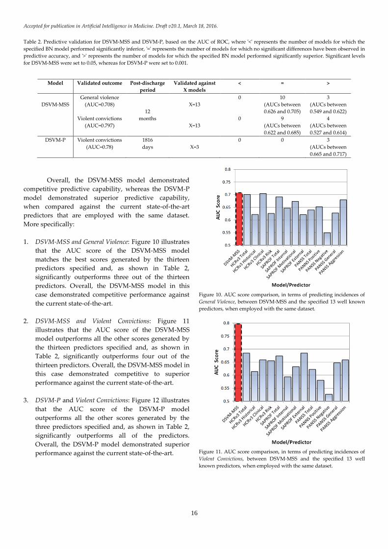
1. DSVM-MSS and General Violence: Figure 10 illustrates
that the AUC score of the DSVM-MSS model
matches the best scores generated by the thirteen
predictors specified and, as shown in Table 2,
significantly outperforms three out of the thirteen
predictors. Overall, the DSVM-MSS model in this
case demonstrated competitive performance against
the current state-of-the-art.
2. DSVM-MSS and Violent Convictions: Figure 11
illustrates that the AUC score of the DSVM-MSS
model outperforms all the other scores generated by
the thirteen predictors specified and, as shown in
Table 2, significantly outperforms four out of the
thirteen predictors. Overall, the DSVM-MSS model in
this case demonstrated competitive to superior
performance against the current state-of-the-art.
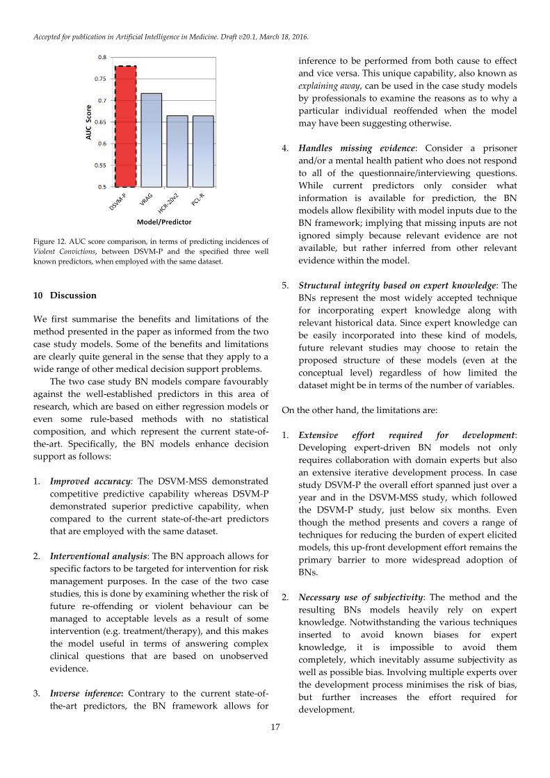
3. DSVM-P and Violent Convictions: Figure 12 illustrates
that the AUC score of the DSVM-P model
outperforms all the other scores generated by the
three predictors specified and, as shown in Table 2,
significantly outperforms all of the predictors.
Overall, the DSVM-P model demonstrated superior
performance against the current state-of-the-art.
Figure 10. AUC score comparison, in terms of predicting incidences of
General Violence, between DSVM-MSS and the specified 13 well known
predictors, when employed with the same dataset.
Figure 11. AUC score comparison, in terms of predicting incidences of
Violent Convictions, between DSVM-MSS and the specified 13 well
known predictors, when employed with the same dataset.
Accepted for publication in Artificial Intelligence in Medicine. Draft v20.1, March 18, 2016.
17
Figure 12. AUC score comparison, in terms of predicting incidences of
Violent Convictions, between DSVM-P and the specified three well
known predictors, when employed with the same dataset.
10 Discussion
We first summarise the benefits and limitations of the
method presented in the paper as informed from the two
case study models. Some of the benefits and limitations
are clearly quite general in the sense that they apply to a
wide range of other medical decision support problems.
The two case study BN models compare favourably
against the well-established predictors in this area of
research, which are based on either regression models or
even some rule-based methods with no statistical
composition, and which represent the current state-of-
the-art. Specifically, the BN models enhance decision
support as follows:
1. Improved accuracy: The DSVM-MSS demonstrated
competitive predictive capability whereas DSVM-P
demonstrated superior predictive capability, when
compared to the current state-of-the-art predictors
that are employed with the same dataset.
2. Interventional analysis: The BN approach allows for
specific factors to be targeted for intervention for risk
management purposes. In the case of the two case
studies, this is done by examining whether the risk of
future re-offending or violent behaviour can be
managed to acceptable levels as a result of some
intervention (e.g. treatment/therapy), and this makes
the model useful in terms of answering complex
clinical questions that are based on unobserved
evidence.
3. Inverse inference: Contrary to the current state-of-
the-art predictors, the BN framework allows for
inference to be performed from both cause to effect
and vice versa. This unique capability, also known as
explaining away, can be used in the case study models
by professionals to examine the reasons as to why a
particular individual reoffended when the model
may have been suggesting otherwise.
4. Handles missing evidence: Consider a prisoner
and/or a mental health patient who does not respond
to all of the questionnaire/interviewing questions.
While current predictors only consider what
information is available for prediction, the BN
models allow flexibility with model inputs due to the
BN framework; implying that missing inputs are not
ignored simply because relevant evidence are not
available, but rather inferred from other relevant
evidence within the model.
5. Structural integrity based on expert knowledge: The
BNs represent the most widely accepted technique
for incorporating expert knowledge along with
relevant historical data. Since expert knowledge can
be easily incorporated into these kind of models,
future relevant studies may choose to retain the
proposed structure of these models (even at the
conceptual level) regardless of how limited the
dataset might be in terms of the number of variables.
On the other hand, the limitations are:
1. Extensive effort required for development:
Developing expert-driven BN models not only
requires collaboration with domain experts but also
an extensive iterative development process. In case
study DSVM-P the overall effort spanned just over a
year and in the DSVM-MSS study, which followed
the DSVM-P study, just below six months. Even
though the method presents and covers a range of
techniques for reducing the burden of expert elicited
models, this up-front development effort remains the
primary barrier to more widespread adoption of
BNs.
2. Necessary use of subjectivity: The method and the
resulting BNs models heavily rely on expert
knowledge. Notwithstanding the various techniques
inserted to avoid known biases for expert
knowledge, it is impossible to avoid them
completely, which inevitably assume subjectivity as
well as possible bias. Involving multiple experts over
the development process minimises the risk of bias,
but further increases the effort required for
development.
Accepted for publication in Artificial Intelligence in Medicine. Draft v20.1, March 18, 2016.
18
3. Complexity: The proposed method should lead to a
minimum number of variables and a conceptually
well-structured and rational model. However,
because the method encourages incorporation of
expert-driven variables (which are additional to
those in the dataset) there is a risk that experts will
over-complicate the model, adding multiple layers of
detailed variables.
Having identified the important limitations of
depending on expert knowledge in almost all of the
development stages, we need to justify its usefulness. It
is important to note that, with the advent of 'big data'
much of the current research on BN development
assumes that sufficient data are available to learn the
underlying BN structure, hence making the expert's
input minimal or even redundant. For example, we could
have made use of:
1. algorithms designed for parameter learning with
insufficient and/or imbalanced data [59];
2. BN learning methods that are appropriate for use
with small datasets but which include a large
number of variables [60];
Making use of such algorithms eliminates, or minimises,
the requirement for expert elicitation. This is very
convenient in the sense that a BN model can be
generated without much effort since we can skip the
process of knowledge elicitation, which is extremely time
consuming since it typically requires collaboration with
multiple domain experts.
Conversely, the method illustrated in this paper
involves extensive use of expertise, in almost all of the
development stages, which greatly increases the effort
required. This is because:
1. Modelling information that matters: We propose
that the starting point of a decision support model is
to determine what information we really require for
inference, rather than generating a model based on
what data is available. This is particularly important
for the two case studies covered in this paper. This is
because the available data is mostly represented by
responses to questions rather than hard facts, and
this causes numerous other decision support
problems (see points 3 and 4 below).
2. Poor quality data means meaningless BN structure:
As discussed in Section 2, our case studies were
based on datasets consisting of thousands of
variables, but the sample sizes of those variables was
below 1,000. To address this problem, the experts
identified (in each case study) less than 100 model
factors as a requirement in order to construct a
comprehensive BN.
On the other hand, if we were to make use of a
structure learning algorithm we would have ended
up with a extensively large network of associations
between hundreds/thousands of responses as
recorded from questionnaires and interviews. Even
when these available responses represent
information that associates with all of the ideal
variables identified for inference, there is typically
far too many variables and far too few samples in
many medical applications to achieve any sensible
structural learning with the state-of-the-art
algorithms; especially in the case of complex and
imbalanced data [61].
Using a structure learning algorithm in these
scenarios results in models that may be superficially
objective, but with a BN structure that is optimised
for some features in the data. This is especially
problematic when the structure is learned on biased
datasets, which is a common challenge in healthcare
settings with well-known inconsistencies in
recording data.
3. Interventional modelling and risk management: A
number of interventions are typically available to the
clinicians and probation officers for managing
relevant risks of interests. The resulting BNs from
this study provide this capability to the decision
makers based on the framework described in Section
7. A BN model learned purely from data in these
scenarios will fail to capture the necessary
underlying dependency structure in situations where
interventions and controls for risk management are
not captured by historical data. However, even if the
historical data captures factors that represent
interventions, this process still requires careful
elicitation of expertise. This is because we require the
expert/s to indicate which of the variables represent
actual interventions. Furthermore, interventions
need to satisfy specific structural-rules (e.g. Graph
surgery and uncertain interventions). On the basis of
uncertain interventions, we also require expertise to
identify the variables which are responsible for the
uncertainty of an intervention (e.g. responsiveness to
treatment and motivation for treatment).
Furthermore, if we were to generate a BN model
from data, we would have ended up simulating
interventions on questionnaire and interviewing
Accepted for publication in Artificial Intelligence in Medicine. Draft v20.1, March 18, 2016.
19
responses, rather than on more meaningful variables
of interest.
4. Counterfactual modelling: Counterfactual analysis
enables decision makers to compare the observed
results in the real world to those of a hypothetical
world. That is, what actually happened and what
would have happened under some different
scenario. While counterfactual analysis is out of the
scope of this paper, it is worth mentioning that this
type of analysis requires further use of expertise, for
counterfactual modelling purposes, as demonstrated
in [62], and on the basis of the application domains
considered in this paper.
11 Future work
The method is expected to be applicable to any other
application domain which involves making inferences
from data records which represent responses from
questionnaires, surveys and interviews. For example,
marketing is an area where questionnaire and survey
data, as well as free-form data from focus groups and
individual interviews is extensive. Furthermore, just like
the medical domains, marketing decision making also
involves critical intervention actions as covered in the
proposed method. The method presented in this paper
will help in describing a more general method to
systemise the development of effective BNs for decision
analysis in all of those common situations where there is
limited or complex data but access to expert knowledge.
However, in domains such as cancer and
bioinformatics it can be much more complex to retrieve
relevant information from an expert and hence, under
such cases there is an increased risk of a weakly defined
BN model. As a result, for future research we are also
interested in investigating ways to minimise expert
dependency. One possible direction is to enhance
structure learning algorithms, which allow for constrains
based on expert knowledge [16-18, 63], with systematic
rules for interventional risk management and decision
analysis.
Furthermore, our future research directions
include describing a more formal approach to generic
problem framing that seeks to minimise model
redundancy in conjunction with efficient use of expert
knowledge and data. A formalised tool will also be
developed to support these enhancements. These generic
problems are being addressed in the BAYES-
KNOWLEDGE project [64].
12 Conclusions
We have presented a generic, repeatable method for
developing real-world BN models that combine both
expert knowledge and data, when (part of) the data is
based on complex questionnaires and interviews with
patients that is available in medical problems.
The method is described in six primary steps: a)
Model objectives, b) BN structure, c) Data management, d)
Parameter learning, e) Interventional modelling, and f)
Structural validation. We have demonstrated how the
incorporation of expert knowledge, along with relevant
historical data, becomes necessary in an effort to provide
decision makers with a model that goes beyond the
predictive accuracy and into usefulness for risk
management through intervention and enhanced
decision support.
While most of the components of the method are
based on established work, the novelty of the method is
that it provides a rigorous consolidated and generalised
framework that addresses the whole life-cycle of BN
model development. This development process is
applicable to any application domain which involves
decision analysis based on complex information, rather
than based on data with hard facts, and in conjunction
with the incorporation of expert knowledge for decision
support via intervention. The novelty extends to
challenging the decision scientists to reason about
building models based on what information is really
required for inference, rather than based on what data is
available.
While the method requires an extensive iterative
process between decision scientists and domain experts,
BNs clearly offer potential for transformative
improvements. The up-front development effort remains
the primary barrier to more widespread adoption of BNs.
The method presents and covers a range of techniques
for reducing the burden of expert elicited models, and
planned research directions will investigate ways to
minimise expert dependency without damaging the
decision support benefits illustrated in this paper.
Although the method is the primary
contribution, it is important to note that the resulting
BNs in the case studies are, to our knowledge, the first
instances of BN models in forensic psychiatry for the
purposes of violence prevention management in the
decision making of released prisoners and mentally ill
patients discharged from MSS.
In validating the method, we have shown that
while both BN applications provide improvements in
predictive accuracy against the current state-of-the-art,
an equally important contribution is the usefulness the
models provide in terms of decision support (an
Accepted for publication in Artificial Intelligence in Medicine. Draft v20.1, March 18, 2016.
20
increasingly important criteria for models in medical
informatics). Although the method was proposed and
evaluated in a forensic medical setting, it is still expected
to be applicable to any other real-world scenario, such as
marketing, where BN models are required for decision
support, where a) part of the data is based on complex
questionnaire, survey, and interviewing data, and b)
decision making involves the simulation of interventions
on inferences as generated on the basis of such complex
data, and in conjunction with expert knowledge.
Acknowledgements
We acknowledge the financial support by the European
Research Council (ERC) for funding this research project,
ERC-2013-AdG339182-BAYES_KNOWLEDGE, and
Agena Ltd for software support. We also acknowledge
the expert input provided by Dr Mark Freestone and
Professor Jeremy Coid in developing the two Bayesian
network applications, which are based on the method
presented in this paper, but which are described in two
other papers [10, 11].
References
[1] Cooper, G. F. (1990). The computational complexity of
probabilistic inference using Bayesian Belief Networks. Artificial
Intelligence, 42(2-3), 393–405.
[2] Pearl J. (1988). Probabilistic reasoning in intelligent systems: networks
of plausible inference. San Mateo, CA: Morgan Kaufmann
Publishers.
[3] Heckerman, D. E., Mamdani, A., & Wellman, M. P. (1995). Real-
World Applications of Bayesian Networks - Introduction.
Communications of the ACM, 38: 24-6.
[4] Jensen, F. V. (1996). An Introduction to Bayesian Networks. Springer,
New York.
[5] Fenton, N.E., & Neil, M. (2012). Risk Assessment and Decision
Analysis with Bayesian Networks. Chapman and Hall, London.
[6] Heckerman, D. E., Horvitz, E. J., Nathwani, B. N. (1992). Towards
normative expert systems. I. The Pathfinder project. Methods of
Information in Medicine, 31: 90–105.
[7] Díez, F. J., Mira, J., Iturralde, E., & Zubillaga, S. (1997). DIAVAL, a
Bayesian expert system for echocardiography. Artificial Intelligence
in Medicine, 10 (1): 59–73.
[8] Nikovski, D. (2000). Constructing Bayesian networks for medical
diagnosis from incomplete and partially correct statistics. IEEE
Transaction on Knowledge and Data Engineering, 12, 4: 509-516.
[9] Yet, B., Perkins, Z., Fenton, N., Tai, N. & Marsh, W. (2013). Not just
data: A method for improving prediction with knowledge. Journal
of biomedical informatics, 48:28-37.
[10] Constantinou, A. C., Freestone, M., Marsh, W., Fenton, N. & Coid,
J. (2015). Risk assessment and risk management of violent
reoffending among prisoners. Expert Systems with Applications,
42(21): 7511-7529.
[11] Constantinou, A. C., Freestone, M., Marsh, W., & Coid, J. (2015).
Causal inference for violence risk management in Forensic
Psychiatry. Decision Support Systems, 80: 42-55.
[12] Spiegelhalter, D. J., Abrams, K. R., & Myles, J. P. (2004). Bayesian
Approaches to Clinical Trials and Health-care Evaluation. John Wiley
and Sons, England.
[13] Pearl J. (2009). Causality: Models, Reasoning and Inference. 2nd
edition, Cambridge University Press, UK.
[14] Constantinou, A. C., Fenton, N. E. & Neil, M. (2012). pi-football: A
Bayesian network model for forecasting Association Football
match outcomes. Knowledge-Based Systems, 36: 322, 339.
[15] Constantinou, A. C., Fenton, Norman E. & Neil, M. (2013).
Profiting from an inefficient Association Football gambling
market: Prediction, Risk and Uncertainty using Bayesian
networks. Knowledge-Based Systems, 50: 60-86.
[16] Zhou, Y., Fenton, N., & Neil, M. (2014). Bayesian network
approach to multinomial parameter learning using data and
expert judgments. International Journal of Approximate Reasoning,
55(5), 1252-1268.
[17] Zhou, Y., Fenton, N. E., & Neil, M. (2014). An Extended MPL-C
Model for Bayesian Network Parameter Learning with Exterior
Constraints. In L. van der Gaag & A. J. Feelders (Eds.), Probabilistic
Graphical Models: 7th European Workshop. PGM 2014, Utrecht. The
Netherlands, September 17-19, 2014 (pp. 581–596). Springer
Lecture Notes in AI 8754.
[18] Zhou, Y., & Fenton, N. E. (2015). An Empirical Study of Bayesian
Network Parameter Learning with Monotonic Causality
Constraints. International Journal of Approximate Reasoning, In press
2015.
[19] Blodgett, J. G., & Anderson, R. D. (2000). A Bayesian Network
Model of the Consumer Complaint Process. Journal of Service
Research, 2 (4): 321-338.
[20] Sebastiani, P., & Ramoni, M. (2001). On the use of Bayesian
networks to analyze survey data. Research in Official Statistics, 4 (1):
53-64.
[21] Ronald, A., Mackoy, R., Thompson, V. B., & Harrell, G. (2004). A
Bayesian Network Estimation of the Service-Profit Chain for
Transport Service Satisfaction. Decision Sciences, 35 (4): 665-689.
[22] Salini, S., & Kenett, R. S. (2009). Bayesian networks of customer
survey satisfaction survey data. Journal of Applied Statistics, 36 (11):
1177-1189.
[23] Ishino, Y. (2014). Knowledge Extraction of Consumers' Attitude
and Behavior: A Case Study of Private Medical Insurance Policy in
Japan. The 8th International Conference on Knowledge Management in
Organizations. Springer Proceedings in Complexity, 425-438.
[24] Heckerman, D. E., & Nathwani, B. N. (1992). Towards normative
expert systems. II. Probability-based representations for efficient
Accepted for publication in Artificial Intelligence in Medicine. Draft v20.1, March 18, 2016.
21
knowledge acquisition and inference. Methods of Information in
Medicine, 31: 106–16.
[25] Andreassen S., Riekehr C., Kristensen B., Schønheyder, H. C.,
Leibovici L. (1999). Using probabilistic and decision theoretic
methods in treatment and prognosis modelling. Artificial
Intelligence in Medicine, 15: 121–34.
[26] Lucas, P. J. F., De Bruijn, N. C., Schurink, K., & Hoepelman, I. M.
(2009). A probabilistic and decision-theoretic approach to the
management of infectious disease at the ICU. Artificial Intelligence
in Medicine, 19 (3): 251–79.
[27] van der Gaag, L. C., Renooij, S., Witteman, C. L., Aleman, B. M.,
Taal, B. G. (2002). Probabilities for a probabilistic network: a case
study in oesophageal cancer. Artificial Intelligence in Medicine, 25:
123–148.
[28] Yet B., Bastani K., Raharjo H., Lifvergren S., Marsh W., & Bergman
B. (2013). Decision Support System for Warfarin Therapy
Management using Bayesian Networks. Decision Support Systems,
55(2): 488-498.
[29] Fenton, N., Neil, M., & Caballero, J. G. (2007). Using Ranked nodes
to model qualitative judgments in Bayesian Networks. IEEE
Transactions on Knowledge and Data Engineering, 19 (10): 1420-1432.
[30] Nielsen, T. D., & Jensen, F. V. (2007). Bayesian networks and decision
graphs. Springer-Verlag New York.
[31] Kuipers, B., Moskowitz, A. J., Kassirer, J. P. (1988). Critical
decisions under uncertainty: Representation and structure.
Cognitive Science, 12: 177–210.
[32] van der Gaag, L. C., Renooij, S., Witteman, C. L. M., Aleman, B., &
Taal, B. G. (1999). How to elicit many probabilities. In: Proceedings
of the 15th International Conference on Uncertainty in Artificial
Intelligence, San Francisco, CA: Morgan Kaufmann, 647–54.
[33] Renooij, S. (2001). Probability elicitation for belief networks: issues
to consider. Knowledge Engineering Review, 16 (3): 255–69.
[34] Druzdzel, M. J., & van der Gaag, L. C. (1995). Elicitation of
Probabilities for Belief Networks: Combining Qualitative and
Quantitative Information. Proc 11th Ann Conf on Uncertainty in
Artificial Intelligence (UAI-05), 141-148, Montreal, Quebec, Canada,
August.
[35] O'Hagan, A., Buck, C. E., Daneshkhah, A., Eiser, J. R., Garthwaite,
P. H., Jenkinson, et al. (2006). Uncertain Judgments: Eliciting Experts'
Probabilities. Wiley, Chichester.
[36] Johnson, S. R., Tomlinson, G. A., Hawker, G. A., Granton, J. T.,
Grosbein, H. A., & Feldman, B. M. (2010). A valid and reliable
belief elicitation method for Bayesian priors. Journal of Clinical
Epidemiology, 63(4): 370-383.
[37] Hubbard, D., & Drummond, D. (2014). How to Measure Anything:
Finding the Value of "Intangibles" in Business. Wiley, New York.
[38] Lin, J., & Haug, P. (2008). Exploiting missing clinical data in
Bayesian network modelling for predicting medical problems.
Journal of Biomedical Informatics, 41: 1-14.
[39] Little, R. J.A., & Rubin, D. B. (2002). Statistical analysis with
missing data. 2nd Edition. Wiley-Interscience, New Jersey.
[40] Enders, C. K. (2006). A primer on the use of modern missing-data
methods in psychosomatic medicine research. Psychosomatic
Medicine, 68:427–36.
[41] Lauritzen, S. L. (1995). The EM algorithm for graphical association
models with missing data. Computational Statistics & Data Analysis,
19: 191-201.
[42] GeNIe & SMILE. (1998). Graphical Network Interface GeNIe &
SMILE. https://dslpitt.org/genie/index.php/about (Accessed: 3
November, 2015).
[43] Lacave, C., Luque, M., & Diez, F. J. (2007). Explanation of Bayesian
Networks and Influence Diagrams in Elvira. IEEE Transactions on
Systems, Man., and Cybernetics - Part B: Cybernetics, 37 (4): 952-965.
[44] Spirtes, P., Glymour, C., & Scheines, R. (1993). Causation, prediction,
and search. Springer, New York.
[45] Woodward, J. (2003). Making things happen. A theory of causal
explanation. Oxford University Press,.
[46] Hagmayer, Y., Sloman, S. A., Lagnado, D. A., & Waldmann, M. R.
(2007). Causal reasoning through intervention. In Causal learning:
Psychology, philosophy and computation, ed. A. Gopnik & L. Schulz.
Oxford University Press, Oxford, England.
[47] Korb, K., Hope, L., Nicholson, A., & Axnick, K. (2004). Varieties of
causal intervention. In Pacific Rim Conference on AI, 2014.
[48] Eaton, D., & Murphy, K. (2007). Exact Bayesian structure learning
from uncertain interventions. In AI & Statistics, 2007.
[49] Agena. (2015). Agena: Bayesian Network and Simulation Software
for Risk Analysis and Decision Support.
http://www.agenarisk.com (Accessed: 7 November, 2015).
[50] Coupe, V. M. H., & van der Gaag, L. C. (2000). Sensitivity analysis:
an aid for probability elicitation. Knowledge Engineering Review, 15:
215–32.
[51] van der Gaag, L. C., & Renooij, S. (2001). Analysing sensitivity
data. In: Proceedings of the 17th International Conference on
Uncertainty in Artificial Intelligence. San Francisco, CA: Morgan
Kaufmann, 530–7.
[52] Hanley, J. A., & McNeil, B. J. (1982). The meaning and use of the
area under a receiver operating characteristic (ROC) curve.
Radiology, 143: 29–36.
[53] Douglas, K. S., Hart, S. D., Webster, C. D., & Belfrage, H. (2013).
HCR-20V3: Assessing Risk of Violence – User Guide. Mental Health,
Law, and Policy Institute, Simon Fraser University, Burnaby,
Canada.
[54] Webster, C.D., Douglas, K.S., Eaves, D.E. & Hart, S.D. (1997). HCR-
20: Assessing Risk for Violence, Version 2. Simon Fraser University,
Vancouver, BC.
[55] de Vries Robbé, M., de Vogel, V., & de Spa, E. (2011). Protective
factors for violence risk in forensic psychiatric patients. A
retrospective validation study of the SAPROF. International Journal
of Forensic Mental Health, 10, 178-186.
[56] Kay, S.R., Fiszbein, A., & Opler, L.A. (1987). The Positive and
Negative Syndrome Scale (Panss) for Schizophrenia. Schizophrenia
Bulletin, 13, 261-276.

Accepted for publication in Artificial Intelligence in Medicine. Draft v20.1, March 18, 2016.
22
[57] Quinsey, V.L. (1998) Violent Offenders – Appraising and Managing
Risk. American Psychological Association, Washington, DC.
[58] Hare, R. D. (2003). Manual for the Hare Psychopathy Checklist-
Revised: 2nd Edition. MultiHealth Systems, Toronto, Canada.
[59] Chawla, N. V., Bowyer, K. W., Hall, L. O., & Kegelmeyer, W. P.
(2002). SMOTE: Synthetic Minority Over-sampling Technique.
Journal of Artificial Intelligence Research, 16: 321-357.
[60] Tsamardinos, I., Aliferis, C. F., Statnikov, A., Brown, L. E. (2003).
Scaling-up Bayesian Network Learning to Thousands of Variables
Using Local Learning Technique. Technical Report DSL-TR-03-02,
Mar. 2003.
[61] He, H., & Garcia, E. A. (2009). Learning from Imbalanced Data.
IEEE Transactions on Knowledge and Data Engineering, 21(9),
1263-1284.
[62] Constantinou, A. C., Yet, B., Fenton, N., Neil, M., & Marsh, W.
(2015). Value of Information analysis for Interventional and
Counterfactual Bayesian networks in Forensic Medical Sciences.
To appear in Artificial Intelligence in Medicine, 2015.
[63] de Campos, C. P., & Ji, Q. (2011). Efficient Structure Learning of
Bayesian Networks using Constraints. Journal of Machine Learning
Research, 12: 663-689.
[64] Fenton, N. (2014). Effective Bayesian Modelling with Knowledge
Before Data (Short Name: BAYES-KNOWLEDGE).
https://www.eecs.qmul.ac.uk/~norman/projects/B_Knowledge.ht
ml (Accessed: 7 October, 2015).
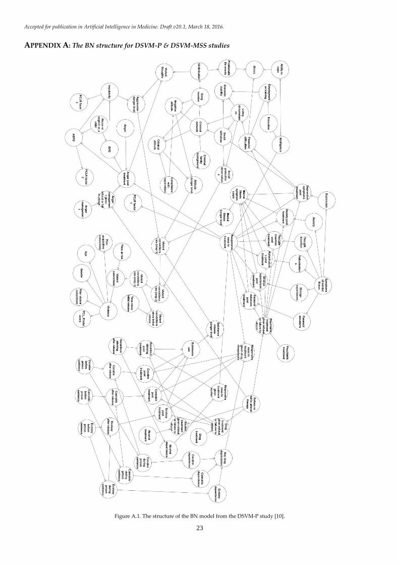
Accepted for publication in Artificial Intelligence in Medicine. Draft v20.1, March 18, 2016.
23
APPENDIX A: The BN structure for DSVM-P & DSVM-MSS studies
Figure A.1. The structure of the BN model from the DSVM-P study [10].
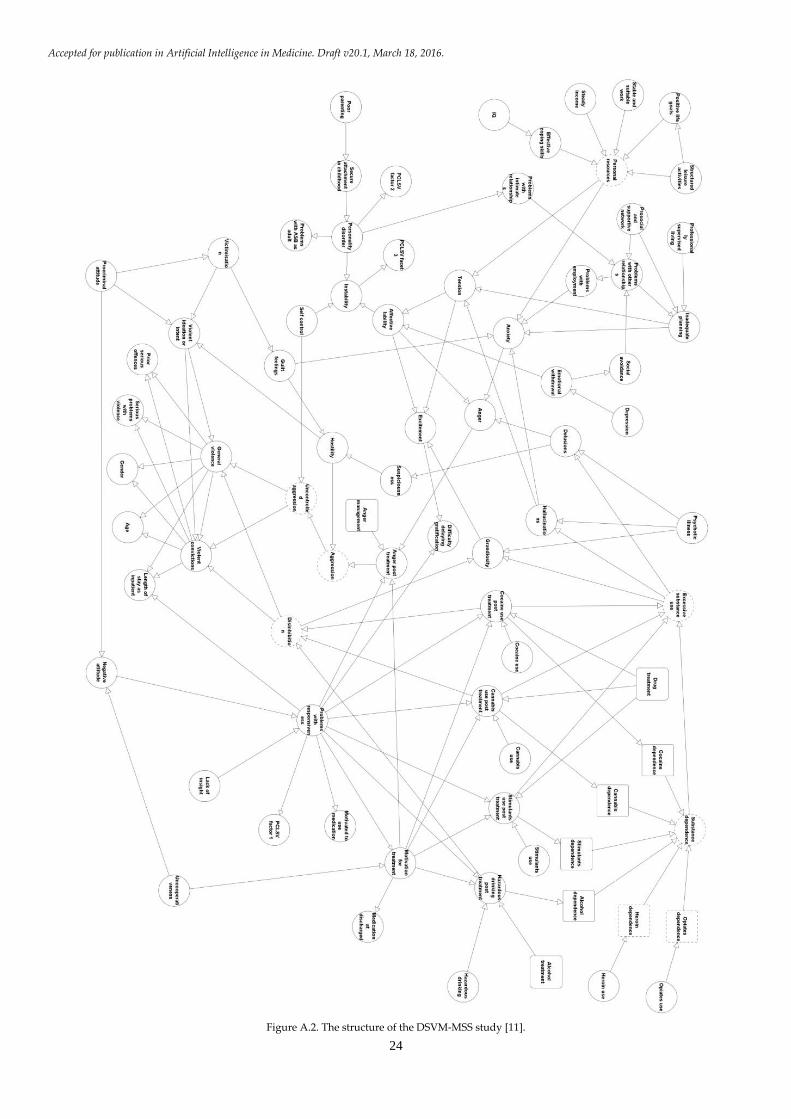
Accepted for publication in Artificial Intelligence in Medicine. Draft v20.1, March 18, 2016.
24
Figure A.2. The structure of the DSVM-MSS study [11].

Accepted for publication in Artificial Intelligence in Medicine. Draft v20.1, March 18, 2016.
25
APPENDIX B: The BN model variables that have been downgraded in terms of complexity
Table B.1. The BN model variables, from both the DSVM-P and DSVM-MSS studies, that have been downgraded, in terms of complexity, in order to
reduce the risk of model overfitting as a result of limited data.
Model Model variable Values from data States in the BN
DSVM-MSS Age 18 to 64 years 18-21/22-25/26-29/30-34/35-39/40-49/50-59/60+
DSVM-MSS Prior serious offences 0 to max None/One/2+
DSVM-MSS Length of stay as inpatient 7 to 7299 days Up to 1 year/Up to 2 years/Up to 5 years/5+ years
DSVM-MSS PCLSVF1 Score 1 to 12 Low=0-1, Medium=2-5, High=6+
DSVM-MSS PCLSVF2 Score 1 to 12 Low=0-1, Medium=2-5, High=6+
DSVM-MSS PCLSVF3 Score 1 to 6 Low=0-1, Medium=2-3, High=4+
DSVM-MSS IQ Score 0 to max Low average/Average/High average
DSVM-MSS Uncooperativeness Score from 1 to 7 No=1, Partly=2-4, Yes=5+
DSVM-MSS Social avoidance Score from 1 to 7 No=1, Partly=2-4, Yes=5+
DSVM-MSS Tension Score from 1 to 7 No=1, Partly=2-4, Yes=5+
DSVM-MSS Guilt feelings Score from 1 to 7 No=1, Partly=2-4, Yes=5+
DSVM-MSS Affective lability Score from 1 to 7 No=1, Partly=2-4, Yes=5+
DSVM-MSS Anger Score from 1 to 7 No=1, Partly=2-4, Yes=5+
DSVM-MSS Excitement Score from 1 to 7 No=1, Partly=2-4, Yes=5+
DSVM-MSS Suspiciousness Score from 1 to 7 No=1, Partly=2-4, Yes=5+
DSVM-MSS Hostility Score from 1 to 7 No=1, Partly=2-4, Yes=5+
DSVM-MSS Difficulty delaying
gratification
Score from 1 to 7 No=1, Partly=2-4, Yes=5+
DSVM-MSS Emotional withdrawal Score from 1 to 7 No=1, Partly=2-4, Yes=5+
DSVM-MSS Delusions Score from 1 to 7 No=1, Partly=2-4, Yes=5+
DSVM-MSS Hallucination Score from 1 to 7 No=1, Partly=2-4, Yes=5+
DSVM-MSS Grandiosity Score from 1 to 7 No=1, Partly=2-4, Yes=5+
DSVM-MSS Anxiety Score from 1 to 7 No=1, Partly=2-4, Yes=5+
DSVM-MSS Depression Score from 1 to 7 No=1, Partly=2-4, Yes=5+
DSVM-P Age 18 to 75 years 18-19/20-21/22-25/ 26-29/30-34/35-39/ 40-49/50-59/60+
DSVM-P Domestic stability a) Frequent address change:
Integer,
b) Eviction: Boolean,
c) Family/friends
unsupportive: Score 1 to 10.
a) Frequent address change: No=0-3, Yes=4+,
b) Eviction: No=false, Yes=true,
c) Family/friends unsupportive: No=0-3, Yes=4+.
Rule introduced: if at least two of the three variables above
returns Yes, then Domestic stability=Low, otherwise Domestic
stability=High.
DSVM-P Financial difficulties a) Behind paying bills: Boolean,
b) Services cut off: Boolean,
c) Low income: Score from 0 to
max.
a) Behind paying bills: No=false, Yes=true,
b) Services cut off: No=false, Yes=true,
c) Low income: No=50+, Yes=0-49.
Rule introduced: if at least one of the three variables above
returns Yes, then Financial difficulties=Yes, otherwise Financial
difficulties=No.
DSVM-P Hazardous drinking Alcohol use disorder
identification test (AUDIT): Score
0 to 32.
No=0-1, Yes=8+
DSVM-P Problematic life events a) Separation/divorce: Boolean,
b) Problems with
friends/family/neighbour:
Boolean,
c) Redundant/sucked: Boolean.
a) Separation/divorce: No=false, Yes=true,
b) Problems with friends/family/neighbour: No=false,
Yes=true,
c) Redundant/sucked: No=false, Yes=true,
Rule introduced: if at least one of the three variables above
returns Yes, then Problematic life events=Yes, otherwise
Problematic life events=No.
DSVM-P Stress High stress score 0 to max No=0-17, Yes=18+
DSVM-P Intelligence IQ Score 0 to 130 Extremely Low/ Borderline/ Low Average/Average/ High
Average/Superior
DSVM-P Criminal network a) Family/friends have criminal
convictions: Boolean,
b) Family/friends offered
a) Family/friends have criminal convictions: No=false,
Yes=true,
b) Family/friends offered drugs: No=false, Yes=true,

Accepted for publication in Artificial Intelligence in Medicine. Draft v20.1, March 18, 2016.
26
drugs: Boolean,
c) Family/friends asked for
money/goods through crime:
Boolean,
d) Family/friends suggested to
commit a crime: Boolean,
e) Family/friends got into a
fight: Boolean.
c) Family/friends asked for money/goods through crime:
No=false, Yes=true,
d) Family/friends suggested to commit a crime: No=false,
Yes=true,
e) Family/friends got into a fight: No=false, Yes=true,
Rule introduced: if at least one of the five variables above
returns Yes, then Criminal network=Yes, otherwise Criminal
network=No.
DSVM-P Criminal attitude a) OK to steal if very poor:
Score 1 to 5,
b) OK to steal from the rick:
Score 1 to 5,
c) OK to steal from shops that
make lots of money: Score 1
to 5,
d) Sometimes it is OK to break
the law: Score 1 to 5,
a) OK to steal if very poor: No=0-1, Yes=2+,
b) OK to steal from the rick: No=0-1, Yes=2+,
c) OK to steal from shops that make lots of money: No=0-1,
Yes=2+,
d) Sometimes it is OK to break the law: No=0-1, Yes=2+.
Rule introduced: if at least one of the four variables above
returns Yes, then Criminal attitude=Yes, otherwise Criminal
attitude=No.
DSVM-P Victimisation a) Victim of theft/burglary:
Boolean,
b) Victim of threats: Boolean,
c) Assaulted: Boolean.
a) Victim of theft/burglary: No=false, Yes=true,
b) Victim of threats: No=false, Yes=true,
c) Assaulted: No=false, Yes=true.
Rule introduced: if at least one of the three variables above
returns Yes, then Criminal network=Yes, otherwise Criminal
network=No.
DSVM-P Compliance with supervision Number of appointments missed
with probation officer: Score 0 to
max
No=1+, Yes=0.
DSVM-P Anger STAXI trait score: Score 0 to 27 No=0-2, Yes=3+.
DSVM-P Cocaine (applies to all three
cocaine variables; before,
during and post-release)
a) Cocaine powder: Boolean,
b) Crack cocaine: Boolean,
a) Cocaine powder: No=false, Yes=true,
b) Crack cocaine: No=false, Yes=true,
Rule introduced: if at least one of the two variables above
returns Yes, then Cocaine=Yes, otherwise Cocaine=No.
DSVM-P Responsiveness to treatment a) Not taken medication:
Boolean,
b) Missed injections: Boolean,
a) Not taken medication: No=false, Yes=true,
b) Missed injections: No=false, Yes=true,
Rule introduced: if one of the two variables above returns Yes,
then Responsiveness to treatment=Partly, if two of the variables
above return Yes, then Responsiveness to treatment=No,
otherwise Responsiveness to treatment=Yes.
DSVM-P PCLR Total score PCL-R: Score 0 to 35 0-9/10-16/17-26/27+
DSVM-P Prior convictions Score 0 to max 0/1/2-5/6+
DSVM-P Prior acquisitive crime
convictions
Score 0 to max 0-2/3-12/13+
Top Related