


Languages
Pages
Legal

物 理 化 学 学 报
Acta Phys. -Chim. Sin. 2018, 34 (10), 1163–1170 1163
Received: December 25, 2017; Revised: February 2, 2018; Accepted: February 19, 2018; Published online: February 27, 2018. *Corresponding authors. Email: [email protected]; Tel./Fax: +81-52-788-6213 (N.Y.). Email: [email protected];
Tel./Fax: +81-52-789-5829 (S.O.).
This work was supported by FLAGSHIP2020, MEXT within Priority Study 5 (Development of New Fundamental Technologies for High-Efficiency Energy
Creation, Conversion/Storage and Use) Using Computational Resources of the K Computer Provided by the RIKEN Advanced Institute for Computational
Science through the HPCI System Research Project (hp170241). This work was also funded by MEXT KAKENHI Grant Number 17K04758 (N.Y.).
© Editorial office of Acta Physico-Chimica Sinica
[Article] doi: 10.3866/PKU.WHXB201802271 www.whxb.pku.edu.cn
Free Energy Change of Micelle Formation for Sodium Dodecyl Sulfate from a Dispersed State in Solution to Complete Micelles along Its Aggregation Pathways Evaluated by Chemical Species Model Combined with Molecular Dynamics Calculations
YOSHII Noriyuki 1,2,*, KOMORI Mika 2, KAWADA Shinji 2, TAKABAYASHI Hiroaki 2, FUJIMOTO Kazushi 2, OKAZAKI Susumu 1,2,*
1 Center for Computational Science, Graduate School of Engineering, Nagoya University, Nagoya 464-8603, Japan. 2 Department of Applied Chemistry, Nagoya University, Nagoya 464-8603, Japan.
Abstract: Surfactant molecules, when dispersed in solution, have been shown
to spontaneously form aggregates. Our previous studies on molecular dynamics
(MD) calculations have shown that ionic sodium dodecyl sulfate molecules
quickly aggregated even when the aggregation number is small. The
aggregation rate, however, decreased for larger aggregation numbers. In
addition, studies have shown that micelle formation was not completed even
after a 100 ns-long MD run (Chem. Phys. Lett. 2016, 646, 36). Herein, we
analyze the free energy change of micelle formation based on chemical species
model combined with molecular dynamics calculations. First, the free energy
landscape of the aggregation, ∆G†i+j, where two aggregates with sizes i and j
associate to form the (i + j)-mer, was investigated using the free energy of
micelle formation of the i-mer, Gi†, which was obtained through MD calculations.
The calculated ∆G†i+j was negative for all the aggregations where the sum of DS
ions in the two aggregates was 60 or less. From the viewpoint of chemical equilibrium, aggregation to the stable micelle is
desired. Further, the free energy profile along possible aggregation pathways was investigated, starting from small
aggregates and ending with the complete thermodynamically stable micelles in solution. The free energy profiles, G(l, k), of
the aggregates at l-th aggregation path and k-th state were evaluated by the formation free energy i ii
n Gl,k † and the
free energy of mixing i i
i
n k Tlnl,k l,k ln ,n kB( ) ( ( ) / ( )) , where ni(l, k) is the number of i-mer in the system at the l-th
aggregation path and k-th state, with i
i
l,k ln ,k= n . All the aggregation pathways were obtained from the initial
state of 12 pentamers to the stable micelle with i = 60. All the calculated G(l, k) values monotonically decreased with
increasing k. This indicates that there are no free energy barriers along the pathways. Hence, the slowdown is not due to
the thermodynamic stability of the aggregates, but rather the kinetics that inhibit the association of the fragments. The time
required for a collision between aggregates, one of the kinetic factors, was evaluated using the fast passage time, tFPT.
The calculated tFPT was about 20 ns for the aggregates with N = 31. Therefore, if aggregation is a diffusion-controlled
process, it should be completed within the 100 ns-simulation. However, aggregation does not occur due to the free energy
barrier between the aggregates, that is, the repulsive force acting on them. This may be caused by electrostatic repulsions
produced by the overlap of the electric double layers, which are formed by the negative charge of the hydrophilic
1164 Acta Physico-Chimica Sinica Vol. 34
groups and counter sodium ions on the surface of the aggregates.
Key Words: Free energy change; Aggregation pathway; SDS; Micelle; Molecular dynamics calculation
1 Introduction Stability of micelles in solution is of great interest in basic
chemistry including the fields of amphiphilic molecular
aggregates, such as biomolecules. A large number of theoretical
and experimental studies have been conducted so far 1–6. First,
regarding the stability of micelles, Tanford 1 and Israelachivili
et al. 2 proposed models based on the attractive force between
hydrophobic groups and repulsive force between hydrophilic
groups. Further, Everette developed a model 3 that incorporates
micellar surface contributions. In addition to these studies,
Blankschtein et al. 4, Oxtoby et al. 5, and Chandler et al. 6
proposed detailed thermodynamic and statistical mechanical
models that include intermolecular interactions of surfactant
molecules. It is now possible to accurately reproduce the free
energy, aggregation number, and critical micelle concentration
(CMC) of the micelles.
From the viewpoint of computational science, the free energy
of micelle formation and micelle size distribution have also
been investigated by molecular dynamics (MD) calculations 7.
Furthermore, using all-atomistic and coarse-grained MD/Monte
Carlo calculations, the aggregation process of surfactant
molecules dispersed in water was examined to evaluate the size
distribution of the aggregates 8–22. We also performed
non-equilibrium MD calculations for anionic sodium dodecyl
sulfate (SDS), cationic dodecyltrimethylammonium chloride
(DTAC), zwitterionic dodecyldimethylamine oxide (DDAO),
and nonionic octaethylene glycol monododecylether (C12E8)
surfactant molecules with an alkyl chain of 12 carbon atoms
and n-dodecane molecules 23,24. The aggregation number, i, of
C12E8 and n-dodecane increased in proportion to the elapsed
time t. This indicates that the aggregation obeys the
Lifshitz-Slyozov (LS) law 25 and is a diffusion-controlled
process. In contrast, the aggregation showed non-LS behavior
for SDS and DTAC (I ∝ t0.3), and for DDAO (I ∝ t0.6).
Among them, formation of stable micelles was completed
smoothly for nonionic C12E8 within 50 ns. However, it was not
completed for ionic SDS and DTAC in spite of the 100-ns-long
MD calculations where a few aggregates composed of several
tens of surfactant molecules remained unassociated with each
other in solution.
In this study, thermodynamic stability is evaluated for the
SDS aggregates of intermediate size on the way to a complete
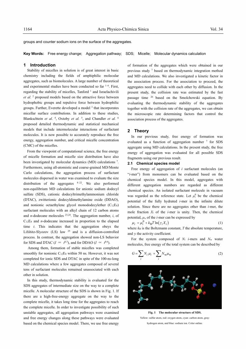
micelle. A molecular structure of the SDS is shown in Fig. 1. If
there are a high-free-energy aggregate on the way to the
complete micelle, it takes long time for the aggregates to reach
the complete micelle. In order to investigate possibility of such
unstable aggregates, all aggregation pathways were examined
and free energy changes along these pathways were evaluated
based on the chemical species model. There, we use free energy
of formation of the aggregates which were obtained in our
previous study 7 based on thermodynamic integration method
and MD calculations. We also investigated a kinetic factor in
the association process. For the association to proceed, the
aggregates need to collide with each other by diffusion. In the
present study, the collision rate was estimated by the fast
passage time 26 based on the Smolchowski equation. By
evaluating the thermodynamic stability of the aggregates
together with the collision rate of the aggregates, we can obtain
the microscopic rate determining factors that control the
association process of the aggregates.
2 Theory In our previous study, free energy of formation was
evaluated as a function of aggregation number 7 for SDS
aggregate using MD calculations. In the present study, the free
energy of aggregation was evaluated for all possible SDS
fragments using our previous result.
2.1 Chemical species model
Free energy of aggregation of i surfactant molecules (an
“i-mer”) from monomers can be evaluated based on the
chemical species model. In this model, aggregates with
different aggregation numbers are regarded as different
chemical species. An isolated surfactant molecule in vacuum
was regarded as the reference state. Let μi0 be the chemical
potential of the fully hydrated i-mer in the infinite dilute
solution. Since there are no aggregates other than i-mer, the
mole fraction Xi of the i-mer is unity. Then, the chemical
potential, μi, of the i-mer can be expressed by
0B lni i i ik T X (1)
where kB is the Boltzmann constant, T the absolute temperature,
and γi the activity coefficient.
For the system composed of Ni i-mers and Nw water
molecules, free energy of the total system can be described by
w wi i
i i
G N N (2)
Fig. 1 The molecular structure of SDS.
Yellow: sulfur atom, red: oxygen atom, cyan: carbon atom, gray:
hydrogen atom, and blue: sodium ion. Color online.

No. 10 doi: 10.3866/PKU.WHXB201802271 1165
where μw is the chemical potential of water.
2.2 Equilibrium mole fraction of i-mer
We assume that the aggregation reaction of one (i − 1)-mer
and one monomer to form one new i-mer occurs reversibly. We
also assume that other aggregates in solution do not change.
Then, the free energy change, ΔG, is expressed using Eqs. (1)
and (2) as
0B B
1 1 1 1ln lni i
ii i
XG k T k T
X X
(3)
where Δμi0 = μi
0 − (μ0i−1 + μ1
0) is the free energy of association
between one (i − 1)-mer and one monomer forming one new
i-mer at infinite dilution (Fig. 2). Δμi0 has already been
evaluated as a function of i by a thermodynamic integration
calculation based on the MD calculation in our previous study 7.
In Table 1, the coefficient ak obtained by fitting the polynomial
0
kk
k
a i to Δμi
0 is listed for two regions (1 ≤ i < 66 and 66 ≤
i ≤ 80).
If the system is in equilibrium, ΔG = 0. Then, the mole
fraction, Xieq, in the equilibrium state satisfies,
eq
eq 0 1 11eq
1
expi ii
ii
XX
X
(4)
as easily derived from Eq. (3).
2.3 Activity coefficient of i-mer
Debye-Hückel (DH) theory is used to evaluate the factor
1 1i
i
in Eq. (4). According to DH theory, lnγi∝i2 for
the activity coefficient γi of ions with i charges 27. Using this expression, we obtain the relationship
B1 1
ln 1i
ik T i
(5)
where the coefficient α was determined such that it reproduces
the experimental critical micelle concentration (CMC) 7.
Regarding Xieq, X1
eq, and α as unknown variables, we obtain
from Eq. (4)
eq eq eq 01 1
2
eq1
2
†
, exp 1
exp
ii
kik
ii
kk
X X X k
X
(6)
where Δμk† = Δμk
0 + α(k−1). Further, we obtain a relation
between CCMC and Xieq
eq eqCMC 1
1
,ii
C iX X
(7)
There are several definitions of CMC using Xieq 28. Here, we
adopted the definition that Xieq satisfies the condition of
eq eq eq1 1( , )iX iX X (8)
at CMC 28, where the total number of molecules belonging to
the aggregate of a certain aggregation number i (≠ 1) is the
same as the total number of molecules of the monomer. Then,
we can determine Xieq, X1
eq, and α numerically using Eqs. (6)–
(8). In the previous study 7, α = −4.5 × 10⁻²² J and X1eq =
0.00015 were obtained, and an aggregation number of i = 57
gave the maximum value of X1eq.
2.4 Free energy of formation of the aggregates
Excess free energy of formation Gi† of the i-mer is the sum of
the free energy of aggregation 0
2
i
k
k
at infinite dilution and
the contribution B1 12
lni
i
ik
k T
of the activity coefficient.
Gi† can be expressed using Δμk
† defined by Eq. (6) as
† †
2
i
i kk
G
(9)
Using this Gi†, Eq. (6) can be rewritten as,
eq
eq†B 1eq
1
exp 1 lnii
XG i k T X
X
(10)
Then, we can obtain the information about the size distribution eq
eq1
iX
X of the i-mer by comparing Gi
† with (i − 1) kBT ln Xieq at
each i.
Fig. 2 Δμi0 and Δμi† as a function of aggregation number i.
The value of Δμi0 obtained from MD calculation is given in Ref. 7. The black solid line
was obtained by fitting the polynomials
0
ka ik
k to the calculated Δμi
0 for two
regions (1 ≤ i < 66 and 66 ≤ i ≤ 80). The red solid line shows Δμi† in Eq. (6),
where the coefficient α was determined to reproduces the experimental CMC.
0 20 40 60 80-1.5
-1
-0.5
0
0.5
i0 ,
i†
(10
-19 J
)
i†
i0
i
Table 1 Fitting coefficients, ak, of Δμi0, where Δμi0 is
approximated as 0
0
kΔμ = a ikik=
.
1 ≤ i ≤ 66 66 ≤ i ≤ 80
a0 4.11 × 10⁻²¹ 7.11 × 10⁻²¹
a1 −5.51 × 10⁻²¹ −4.81 × 10⁻²¹
a2 3.73 × 10⁻²² 1.21 × 10⁻²²
a3 −1.73 × 10⁻²³ −1.21 × 10⁻²⁴
a4 4.24 × 10⁻²⁵ 4.00 × 10⁻²⁷
a5 −5.31 × 10⁻²⁷ −
a5 3.24 × 10⁻²⁹ −
a7 −7.65 × 10⁻³² −

1166 Acta Physico-Chimica Sinica Vol. 34
The excess free energy of aggregation, ΔG†i+j, where two
aggregates with sizes i and j associate to form the (i + j)-mer
can be given by
† † † †i j i j i jG G G G (11)
Then, free energy of aggregation, ΔGi+j, may be obtained by
adding ideal free energy of mixing
eq
mixB eq eq
, lni j
i ji j
XG i j k T
X X
(12)
to the excess free energy of aggregation, Eq. (11), as † mix
i j i ji jG G G (13)
This determines whether the aggregation actually goes
forward or not.
3 Results and discussion In this section, free energy of aggregation of an i-mer and
j-mer to form (i + j)-mer is presented. The free energy profile is
also investigated along aggregation pathways, and then,
kinetics in the final stage of the aggregation is discussed.
3.1 Free energy of micelle formation
As shown in Fig. 2, free energy of micelle formation, Δμi0
and Δμi†, rapidly decrease with increasing i for i ≤ 10. This
stability is caused by the increase of coverage of the aggregate
surface by hydrophilic groups with increasing aggregation
number 29. In contrast, the instability for i ≥ 40 is due to the
decrease of the distance between hydrophilic groups 30.
Fig. 3 shows the free energy of formation, G i†, of the i-mer
calculated by Eq. (9). The G i† shows an inverse S-shaped
function with an inflection point near i = 40 where Δμi† in Fig. 2
has a minimum. The shape of this G i† curve is similar to the
reported model functions of the free energy of micelle
formation 2,3; it is convex upward for 1 ≤ i < 40 and convex
downward for 40 ≤ i ≤ 80. Now, X1eq is constant in the range of
0 < X1 eq < 1, such that (i − 1) kBT ln X1
eq is a monotonically
decreasing linear function of i, as shown in Fig. 3. Probability
that the i-mer is found in the system is determined by the
relative magnitude of both G i† and (i − 1) kBT ln X1
eq, as shown
in Eq. (10). Thus, the aggregates with 1 ≤ i < 40 are not found
because of the condition, G i† − (i − 1) kBT ln X1
eq > 0. In
contrast, the aggregate with 40 ≤ i ≤ 80 must be found in the
system because of the condition G i† − (i − 1) kBT ln X1
eq < 0. G i†
in Fig. 3 shows such tendency, giving a correct micelle size
distribution.
G i† − (i−1) kBT ln X1
eq at several concentrations, C, is plotted
in Fig. 3. Here, we assume that G i† does not depend on C for C <
30 CCMC. For C < CCMC, the minimum is found at i = 1,
indicating that the monomer is present most frequently in the
system. At C = CCMC, local minima are observed at i = 1 and
57, and the monomer and the stable micelle, respectively, are
distributed to a similar extent. For C > CCMC, the minimum at i =
57 decreases as C increases. This indicates that the micelle with
i = 57 becomes more stable and is found more frequently in the
system.
In Fig. 3, there is a broad high free energy region around i =
20. The aggregation between the two aggregates with similar
sizes (i ≈ 20) hardly occurs at CCMC because the probability that
the aggregates with i ~ 20 are found in the system is much
smaller than that with i = 1 and 57. This is consistent with the
Aniansson-Wall model 31, where aggregation proceeds through
the sequential reaction in which the aggregate size increases by
addition of monomers.
3.2 Free energy of aggregation of the i-mer and j-mer
Fig. 4 shows a free energy landscape of aggregation, ΔG†i+j,
of an i-mer and j-mer given by Eq. (11). ΔG†i+j is negative for
all i and j where the two aggregates satisfy i + j ≤ 60. The
aggregation under this condition proceeds thermodynamically.
In particular, ΔG†i+j becomes a large negative value when the
two aggregates are of similar size with i ≈ 30. This is because,
as shown in Fig. 3, the aggregates with i ≈ 30 are greatly
unstable, while the aggregates with i ≈ 60 are quite stable.
In contrast, in the aggregation of the large fragments of i ≥
60 (for example, two 60-mers are fused into one to form a
120-mer), ΔG†i+j has a large positive value. In such an
aggregation, the hydrophilic groups in the formed aggregate
Fig. 3 Aggregation number i dependence of G†i − (i − 1) kBT lnX1
eq.
Gi†: black line, G i
† − (I − 1) kBTlnX1 eq at 0.5CMC, CMC, and 30CMC are depicted by the
blue, red and green lines, respectively. The black dashed line represents (I − 1)
kBT ln X1 eq at CMC. Color online.
0 20 40 60 80-4
-3
-2
-1
0
1
Gi†
(10
-18 J
)
i
Gi† - (i-1)kBTlnX1
eq (0.5CMC) Gi
† - (i-1)kBTlnX1eq (CMC)
Gi† - (i-1)kBTlnX1
eq (30CMC) Gi
†
Fig. 4 Free energy landscape, ΔG†i+j, of formation of
an (i + j)-mer from i-mer and j-mer.

No. 10 doi: 10.3866/PKU.WHXB201802271 1167
become close to each other on the aggregate surface 30. It is
quite unstable.
3.3 Free energy profile along possible aggregation
pathways
We consider free energy profile along possible aggregation
pathways from randomly solved structure to complete spherical
micelles. The aggregation pathways are generated randomly
according to the procedure given in Fig. S1. Here, l is the index
of independent aggregation path, and k represents the state of
the system. Then, the free energy profile, G(l, k), was evaluated
using G i† by,
†B
,, ,
,ln i
i ii
nG n G k T
n
l kl k l k
l k
(14)
where ni(l, k) is the number of i-mer in the system at l-th
aggregation path and k-th state. , ,i
i
l k ln n k is the total
number of aggregates in the system. The free energy of mixing,
Gmix(l, k), was evaluated by,
mixB ln
,, ,
,i
i
i
n lG n k T
kl k l
nk
l k (15)
We started with 12 pentamers as an initial state because the
number of aggregation paths from 60 monomers is too large to
calculate. This initial state is reasonable because at the early
stage of aggregation simulation from the randomly dispersed
molecules, the monomers quickly associated to form small
fragments with a several molecules such as pentamers. Totally
39700 aggregation paths were investigated. 800 randomly
chosen profiles, G(l, k), and the contribution of Gmix(l, k) are
plotted in Fig. 5a.
G(l, k) decreases monotonically with increasing k at all l. The
free energy does not increase with the growth of the aggregates.
Further, the absolute value of Gmix(l, k) is several tens of
kJ·mol−1, whereas that of G(l, k) is several hundreds or one
thousand kJ·mol−1. It is more than one order of magnitude larger
than Gmix(l, k). Thus, †,i ii
n Gl k is a dominant factor in
G(l, k).
Fig. 5b shows increment of the free energy ΔG(l, k) = G(l, k) −
G(l, k − 1) along the path. It is noted that they are all negative
values. Although the positive values were found that in several
ΔGmix(l, k) = Gmix(l, k) − Gmix(l, k − 1), the values are in the
order of several kJ/mol, their contributions to ΔG(l, k) being
quite limited. As a result, ΔG(l, k) is in the range of −50 to
−270 kJ·mol−1. Thus, no barrier is found in the free energy
profile from the initial state to the complete spherical micelles.
3.4 Aggregation simulation
Next, free energy change during spontaneous aggregation of
the fragments was investigated based on the aggregation
simulation. The detail of the aggregation simulation is
described in the supporting information.
Snapshots of SDS aggregates in an aggregation simulation
are shown in Fig. 6. From the trajectory of the aggregation
simulation, fragments were identified using the intermolecular
bond between the DS ions. The contact area between the
hydrophobic parts of the two DS ions was used to define the
bond between the DS ions. Voronoi polyhedra were defined
using all atoms except for hydrogen. The surface of the DS ion
was defined using the Voronoi polyhedra. When the contact
area of the two DS ions is greater than a threshold value, the
two DS ions were regarded as bonded. From the contact area
distribution of two DS ions in the stable SDS micelle, the
threshold was set to be 0.05 nm2 23.
Results of the aggregation simulation are shown in Fig. 7.
The largest aggregation number is plotted in Fig. 7a for
independent six MD runs. The aggregates with i = 10–20 were
quickly formed within several tens of nanoseconds. However,
the aggregation did not proceed more. Four largest aggregation
numbers are plotted as a function of t in Fig. 7b for one
trajectory, green one in Fig. 7a. At t = 30 ns, three aggregates
with aggregation numbers of 12, 19, and 29 were formed.
However, their aggregation numbers hardly changed until t =
100 ns.
The time evolution of the maximum aggregation number
presented here is similar to that of aggregation simulation
performed using different potential parameters (CHARMM 36) 23.
Fig. 5 Free energy profile G(l, k) (lower plot of (a)) and Gmix(l, k) (upper plot of (a)), and ΔG(l, k) (lower plot of (b)) and ΔGmix(l, k) (upper plot of (b))
along the aggregation pathways.
Note that the scales on the vertical axes are different between (a) and (b).

1168 Acta Physico-Chimica Sinica Vol. 34
This indicated that the results do not strongly depend on the
details of potential parameters. In contrast, as described in the
introduction, the time evolution of the maximum aggregation
number greatly differs depending on whether the hydrophilic
group is ionic, zwitterionic or nonionic 24. The electric charge
of the hydrophilic group has a strong influence on the rate of
aggregation.
The time evolution of the free energy G(l, t) was evaluated
by Eq. (14) for each trajectory. For all l, G(l, t) decreases with
increasing time. As described in Section 3.3, it is
thermodynamically stable to form one aggregate. However, the
aggregation was not actually completed during the 100-ns-long
simulation, and the system did not reach the equilibrium state.
A kinetic mechanism is considered to prevent the fragment
from aggregating each other.
3.5 Aggregation kinetics
The kinetics concerned with the aggregation between the
aggregates is dominated by two factors: (1) collision by
diffusion, and (2) crossing the free energy barrier along the
reaction coordinates of the aggregation.
Here, the frequency of collision between the aggregates
caused by diffusion is evaluated to examine whether the 100 ns
long simulation was sufficient for the aggregates to diffuse and
collide each other. For this purpose, we use the fast passage
time, which is often used to evaluate the reaction time in a
diffusion-controlled reaction where the reaction proceeds by
the contact of two spherical particles in solution 26. First, one
aggregate is fixed in space. The range of motion of another
aggregate is assumed to be inside a sphere of radius R centered
on the fixed aggregate, and the area outside the sphere with
radius Rm (< R), which is the sum of the radii of two aggregates
that are fixed and diffusible. Then, the fast passage time, tFPT, is
given by,
2 2 32
FPT 2
1 5 6 3
15 1
x x x xRt
D x x x
(16)
where x = Rm/R. D is the diffusion coefficient of the two
aggregates, and the sum of the self-diffusion coefficients of the
individual aggregates is commonly used. The self-diffusion
coefficient of the individual aggregate was evaluated from the
Einstein-Stokes law (D = kBT/6πηRm), where the viscosity
coefficient, η, of water at 300 K is 0.000853 Pa·s 32, and Rm is
obtained from the radius of gyration by the MD calculation
(1.34 nm at N = 31 33).
The time required for the contact between two aggregates (N =
31) in the aggregation simulation is estimated to be 20 ns from
tFPT. Therefore, several collisions should have occurred in the
last 50–70 ns. However, the aggregation did not occur for all
independent six simulations. Thus, the aggregation is not a
diffusion-controlled process.
A repulsive interaction coming from free energy barrier must
exist between aggregates. The repulsive force may be produced
by the overlap of the electric double layer formed on the
surface of the aggregates by the negative charge of the
surfactant molecules and the positive charge of the counter
ions. More than 100 ns are necessary to pass the free energy
Fig.6 Snapshot of SDS aggregates in solution at elapsed time (a) t = 0 ns, (b) 7 ns, (c) 50 ns, and (d) 100 ns.
Colors for atoms are the same as in Fig. 1. Water molecules are not depicted for clarity.
Fig. 7 Time evolution of (a) maximum aggregation number, i, of
aggregates in the independent six aggregation simulations, (b) four
largest aggregation numbers for one trajectory, green line in Fig. 7a,
and (c) free energy profile G(l, t) of the system evaluated by Eq. (14) for
each trajectory.
Results of the six independent MD runs are plotted in different colors in (a) and (c).

No. 10 doi: 10.3866/PKU.WHXB201802271 1169
barrier by to form the stable micelles.
4 Conclusions In this study, the free energy landscape, ΔG†
i+j, of aggregation
was investigated using the free energy, Gi†, of micelle formation
obtained by MD calculations. This analysis is based on
chemical species model. The calculated ΔG†i+j was negative for
all aggregations where the sum of the number of DS ions in the
two aggregates was 60 or less. From the viewpoint of chemical
equilibrium, aggregation to the stable micelle is desired.
Further, free energy profile along possible aggregation
pathways was investigated from small aggregates to
thermodynamically stable complete micelles in solution. The
free energy profile G(l, k) of the aggregates was evaluated by
†( ),i ii
n Gl k and B
,,
,ln i
i
i
nn k T
n
l kl k
l k . All aggregation
pathways were obtained from the initial state of 12 pentamers
to the stable micelle with i = 60. The calculated G(l, k) all
monotonically decreases with increasing k. The absolute value
of †( ),i i
i
n Gl k was an order of magnitude greater than that
of B
,,
,ln i
i
i
nn k T
n
l kl k
l k , dominating the aggregation
process.
Independent six MD calculations were performed for the
spontaneous aggregation process of SDS dispersed in water. In
each calculation, 10–30-mers were formed within about 20 ns.
However, the aggregation did not proceed more and was not
completed even after 100 ns simulations, despite the fact that
the SDS micelle with i ≈ 60 is the most thermodynamically
stable. For each run, the free energy decreased sharply with
time for the first 20 ns, but hardly changed after that.
The time required for a collision between aggregates was
evaluated using the fast passage time, tFPT. The calculated tFPT
was about 20 ns for the aggregates with N = 31. Thus, if
aggregation is a diffusion-controlled process, the aggregation
should be completed within the 100 ns simulation. However, in
fact, the aggregation does not proceed. This is due to the free
energy barrier between the aggregates, that is, the repulsive
force acting on them. This may be caused by electrostatic
repulsion produced by the overlap of the electric double layers
formed by the negative charge of the hydrophilic groups and
counter sodium ions on the surface of the aggregates. In order
to aggregate to form stable micelles the aggregates are required
to pass this barrier thermally.
The potential of mean force between aggregates must be
evaluated to obtain the time constant for the aggregation of two
aggregates to form the stable micelle 34. We discuss this free
energy barrier elsewhere 35, based on free energy calculation
combined with molecular dynamics calculation.
Acknowledgment: Calculations were mainly performed at
the Research Center for Computational Science, Okazaki,
Japan, partially at the Information Technology Center of
Nagoya University, and partially at the Institute for Solid State
Physics, the University of Tokyo.
Supporting Information: available free of charge via the
internet at http://www.whxb.pku.edu.cn.
References and Notes (1) Tanford, C. J. Phys. Chem. 1974, 78, 2469.
doi: 10.1021/j100617a012
(2) Israelachvili, J. N. Intermolecular and Surface Forces, 2nd ed.;
Academic Press: London, UK, 1992.
(3) Everett, D. H. Basic Principles of Colloid Science; The Royal Society
of Chemistry: London, UK, 1988.
(4) Puvvada, S.; Blankschtein, D. J. Chem. Phys. 1990, 92, 3710.
doi: 10.1063/1.457829
(5) Christopher, P. S.; Oxtoby, D. W. J. Chem. Phys. 2003, 118, 5665.
doi: 10.1063/1.1554394
(6) Maibaum, L.; Dinner, A. R.; Chandler, D. J. Phys. Chem. B 2004,
108, 6778. doi: 10.1021/jp037487t
(7) Yoshii, N.; Iwahashi, K.; Okazaki, S. J. Chem. Phys. 2006, 124,
184901. doi: 10.1063/1.2179074
(8) Pool, R.; Bolhuis, P. G. J. Chem. Phys. 2007, 126, 244703.
doi: 10.1063/1.2741513
(9) Burov, S. V.; Shchekin, A. K. J. Chem. Phys. 2010, 133, 244109.
doi: 10.1063/1.3519815
(10) Verde, A. V.; Frenkel, D. Soft Matter 2010, 6, 3815.
doi: 10.1039/C0SM00011F
(11) Bernardino, K.; de Moura, A. F. J. Phys. Chem. B 2013, 117, 7324.
doi: 10.1021/jp312840y
(12) Marrink, S. J.; Tieleman, D. P.; Mark, A. E. J. Phys. Chem. B 2000,
104, 12165. doi: 10.1021/jp001898h
(13) Lazaridis, T.; Mallik, B.; Chen, Y. J. Phys. Chem. B 2005, 109,
15098. doi: 10.1021/jp0516801
(14) Tieleman, D. P.; van der Spoel, D.; Berendsen, H. J. C. J. Phys.
Chem. B 2000, 104, 6380. doi: 10.1021/jp001268f
(15) Bond, P. J.; Cuthbertson, J. M.; Deol, S. S.; Sansom, M. S. P. J. Am.
Chem. Soc. 2004, 126, 15948. doi: 10.1021/ja044819e
(16) Jusufi, A.; Hynninen, A. -P.; Panagiotopoulos, A. Z. J. Phys. Chem. B
2008, 112, 13783. doi: 10.1021/jp8043225
(17) Sanders, S.; Sammalkorpi, M.; Panagiotopoulos, A. Z. J. Phys. Chem.
B 2012, 116, 2430. doi: 10.1021/jp209207p
(18) Sammalkorpi, M.; Karttunen, M.; Haataja, M. J. Phys. Chem. B 2007,
111, 11722. doi: 10.1021/jp072587a
(19) Cheong, D.; Panagiotopoulos, A. Z. Langmuir 2006, 22, 4076.
doi: 10.1021/la053511d

1170 Acta Physico-Chimica Sinica Vol. 34
(20) Pool, R.; Bolhuis, P. G. J. Phys. Chem. B 2005, 109, 6650.
doi: 10.1021/jp045576f
(21) Pool, R.; Bolhuis, P. G. Phys. Rev. Lett. 2006, 97, 018302.
doi: 10.1103/PhysRevLett.97.018302
(22) Pool, R.; Bolhuis, P. G. Phys. Chem. Chem. Phys. 2006, 8, 941.
doi: 10.1039/B512960E
(23) Kawada, S.; Komori, M.; Fujimoto, K.; Yoshii, N.; Okazaki, S. Chem.
Phys. Lett. 2016, 646, 36. doi: 10.1016/j.cplett.2015.12.062
(24) Fujimoto, K.; Kubo, Y.; Kawada, S.; Yoshii, N.; Okazaki, S. Mol.
Simul. 2017, 43, 13. doi: 10.1080/08927022.2017.1328557
(25) Lifshitz, I. M.; Slyozov, V. V. J. Phys. Chem. Solids 1961, 19, 35.
doi: 10.1016/0022-3697(61)90054-3
(26) Szabo, A.; Schulten, K.; Schulten, Z. J. Chem. Phys. 1980, 72, 4350.
doi: 10.1063/1.439715
(27) Moore, W. J. Physical Chemistry, 4th ed.; Prentice Hall, Inc.: Upper
Saddle River, NJ, USA, 1972.
(28) Everett, D. H. Colloids Surf. 1986, 21, 41.
doi: 10.1016/0166-6622(86)80081-6
(29) Yoshii, N.; Okazaki, S. Chem. Phys. Lett. 2006, 425, 58.
doi: 10.1016/j.cplett.2006.05.004
(30) Yoshii, N.; Okazaki, S. Chem. Phys. Lett. 2006, 426, 66.
doi: 10.1016/j.cplett.2006.05.038
(31) Aniansson, E. A. G.; Wall, S. N. J. Phys. Chem. 1974, 78, 1024.
doi: 10.1021/j100603a016
(32) Kestin, J.; Sokolov, M.; Wakeham, W. A. J. Phys. Chem. Ref. Data
1978, 7, 941. doi: 10.1063/1.555581
(33) The value obtained in Eq. (1) of Ref. 28 was used.
(34) Russel, W. B.; Saville, D. A.; Schowalter, W. R. Colloidal
Dispersions; Cambridge University Press: Cambridge, UK, 1989.
(35) Kawada, S.; Fujimoto, K.; Yoshii, N.; Okazaki, S. J. Chem.
Phys. 2017, 147, 084903. doi: 10.1063/1.4998549
Top Related