


Languages
Pages
Legal

HAL Id: tel-00624760https://tel.archives-ouvertes.fr/tel-00624760
Submitted on 19 Sep 2011
HAL is a multi-disciplinary open accessarchive for the deposit and dissemination of sci-entific research documents, whether they are pub-lished or not. The documents may come fromteaching and research institutions in France orabroad, or from public or private research centers.
L’archive ouverte pluridisciplinaire HAL, estdestinée au dépôt et à la diffusion de documentsscientifiques de niveau recherche, publiés ou non,émanant des établissements d’enseignement et derecherche français ou étrangers, des laboratoirespublics ou privés.
Fractional quantum Hall effect in multicomponentsystems
Zlatko Papic
To cite this version:Zlatko Papic. Fractional quantum Hall effect in multicomponent systems. Condensed Matter [cond-mat]. Université Paris Sud - Paris XI, 2010. English. <tel-00624760>
Universite Paris XI
UFR Scientifique d’Orsay
Fractional quantum Hall effect in multicomponent systems
THESE
presentee a l’Universite Paris XI
pour l’obtention du grade de
Docteur en Sciences de l’Universite de Paris XI Orsay
par
Zlatko PAPIC
de
Belgrad (Serbie)
Soutenue le 23 septembre 2010 devant la Commission d’examen
M. Marc GABAY President de Jury
M. Mark O. GOERBIG Directeur de these
M. Thors Hans HANSSON Rapporteur
M. Milan KNEZEVIC Examinateur
Mme. Milica MILOVANOVIC Directrice de these
M. Zoran RADOVIC Examinateur
M. Nicolas REGNAULT Directeur de these
Numero d’ordre de la these:
9913

2
Abstract
We study a number of fractional quantum Hall systems, such as quantum Hall bi-
layers, wide quantum wells or graphene, where underlying multicomponent degrees
of freedom lead to the novel physical phenomena. In the quantum Hall bilayer at
the filling factor ν = 1 we study mixed composite boson-composite fermion trial
wave functions in order to describe the disordering of the exciton superfluid as the
bilayer distance is increased. We propose wave functions to describe the states of
the bilayer for intermediate distances and examine their properties. At the bilayer
total filling ν = 1/2 and ν = 2/5 we study the quantum phase transition between the
multicomponent Halperin states and the polarized, Abelian and non-Abelian, phases
as the tunneling term is varied. We use a combination of exact diagonalization and
the effective BCS model to study the transitions. Furthermore we introduce a re-
alistic model of the wide quantum well which is used to examine even-denominator
quantum Hall states at ν = 1/2 and ν = 1/4 in the lowest Landau level. Finally, we
explore some possibilities for the fractional quantum Hall effect in graphene based
on the multicomponent picture of spin and valley degrees of freedom.
Apstrakt
U ovoj tezi proucavamo nekoliko primera frakcionog kvantnog Hall-ovog efekta, u
sistemima kao sto su kvantni Hall-ov dvosloj, siroke kvantne jame i grafen, gde
visekomponentni sistemi slobode dovode do novih fizickih fenomena. U slucaju
kvantnog Hall-ovog dvosloja na punjenju ν = 1 proucavamo probne talasne funkcije
koje opisuju mesavinu kompozitnih bozona i kompozitnih fermiona, sa ciljem da
opisemo razuredjenje ekscitonskog superfluida sa povecanjem rastojanja izmedju slo-
jeva. U slucaju dvosloja na punjenju ν = 1/2 i ν = 2/5, proucavamo kvantne fazne
prelaze izmedju visekomponentnih Halperin-ovih stanja i polarizovanih, abelijanskih
i neabelijanskih, faza koje nastaju sa povecanjem tuneliranja. Prelazi su analizirani
pomocu metoda egzaktne dijagonalizacije i efektivnog BCS modela. U nastavku
je uveden realisticni model za siroku kvantnu jamu koji je iskoriscen za ispitivanje
kvantnih Hall-ovih stanja sa parnim imeniocem na punjenju ν = 1/2 i ν = 1/4 u na-
jnizem Landau-ovom nivou. Na kraju, ispitivane su mogucnosti za frakcioni kvantni
Hall-ov efekat u grafenu na osnovu visekomponentnog opisa koji ukljucuje stepene
slobode koju poticu od spina i resetke.
Resume
Nous etudions un certain nombre de manifestations de l’effet Hall quantique frac-
tionnaire dans les bicouches d’effet Hall quantique, des puits quantiques larges ou
le graphene, dans lesquels les degres de liberte multicomposantes produisent des
phenomenes physiques insolites. Dans la bicouche d’effet Hall quantique du remplis-
sage total ν = 1, nous examinons les fonctions d’onde mixtes des bosons composites
et fermions composites afin de decrire la destruction de la suprafluidite excitonique au
fur et a mesure qu’on augmente la distance entre les deux couches. Nous proposons
des fonctions d’onde d’essai qui decriraient bien l’etat de la bicouche quand il s’agit de
distances intermediaires et nous y etudions leurs proprietes. Dans la bicouche d’effet
Hall quantique du remplissage total ν = 1/2 et ν = 2/5, nous etudions la transition
de phase quantique entre les etats multicomposantes de Halperin et les phases po-
larisees (abeliannes et non-abeliannes) en fonction des modifications effectuees dans
le terme tunnel. Afin d’etudier les transitions, nous utilisons a la fois la diagonal-
isation exacte et la theorie effective BCS. Nous presentons d’autre part un modele
realiste du puits quantique large que nous utilisons dans l’examen des etats avec un
denominateur pair, a ν = 1/2 et ν = 1/4 dans le plus bas niveau de Landau. Nous
proposons enfin quelques etats d’effet Hall quantique fractionnaire possibles dans le
graphene, celles-ci reposant sur l’image multicomposante qui concerne les degres de
liberte de spin et de vallee.
Acknowledgements
The work presented here began at the Scientific Computing Laboratory in Belgrade,
under the supervision of Milica Milovanovic. I thank her for the patient guidance
throughout the years of my thesis, for being always attentive to my evolving research
interests and available to discuss physics. I consider myself fortunate that she gave
me the chance to work in the quantum Hall effect, the field I had discovered as an
undergraduate student at the Weizmann Institute doing my internship with Moty
Heiblum, to whom I am thankful for the best possible introduction to the quantum
Hall effect that a theoretician can hope for: through the dirty and complicated
experimental work.
I am furthermore indebted to Milica for having the foresight to realize my difficulty
in learning the numerical tools necessary for the topic I was working on and sharing
her advisorship over my PhD with Mark Goerbig at the Laboratoire de Physique des
Solides in Orsay, and Nicolas Regnault at the Laboratoire Pierre Aigrain at Ecole
Normale Superieure in Paris. I feel enriched by having had the possibility of working
with all of these three great physicists (whom I equally consider my advisors, should
I ever need to quantify that), despite the fact that the numbers of our exchanged
emails could be daunting at times. I also relish the fact that I’ve experienced a new
country and a new culture without having to abandon the place I came from.
I would like to thank Mark for being calm and authoritative when it was needed, for
being always there for practical issues, discussing physics and doing all that with a
unique zest of hedonism. I thank Nicolas for teaching me nearly everything about
exact diagonalization and numerics in general - with a light touch!, running some
of my codes on his cluster and doing some calculations instead of me ;-), as well as
showing me how to be a practical physicist-theoretician.
During the course of my PhD, I attended several great workshops at ICTP Trieste,
SFK conference in Vrsac, Max Planck institute for complex systems, KITP in Santa
Barbara and Nordita in Stockholm, where certain collaborations were initiated. I
would like to especially thank Bogdan Andrei Bernevig for countless discussions and
inspiration by his inimitable way of doing physics in every situation imaginable. I also
thank Sankar Das Sarma for our joint work on wide quantum well problems. I have
furthermore benefitted a great deal from discussing numerics with Karel Vyborny
and Thierry Jolicoeur.
I thank the Scientific Computing Laboratory, Laboratoire de Physique des Solides
and Laboratoire Pierre Aigrain for their hospitality and all the colleagues for making
the work and leisure time enjoyable and fun. A personal note of gratitude goes to
Aleksandar Belic for his continuous support as the head of SCL, as well as to Hans
Hansson and Steve Simon for their proofreading of the manuscript.
This work has been supported in part by the fellowship of the Serbian Ministry of
science, the Marie Curie scholarship for early stage research training in Orsay, the
CNRS fellowship and the fund of Region Ile-de-France for “cotutelle” programs.
Finally, I would like to dedicate this thesis to my family and dear friends whose
support during the last years enabled me to reach this point.
Zlatko Papic

iv
Contents
Nomenclature ix
Foreword xvii
1 Introduction 1
1.1 Fractional quantum Hall effect . . . . . . . . . . . . . . . . . . . . . . . . . . . . 1
1.2 Polarized electrons in the lowest Landau level . . . . . . . . . . . . . . . . . . . . 5
1.2.1 Laughlin’s wave function . . . . . . . . . . . . . . . . . . . . . . . . . . . . 6
1.2.2 Effective field theories . . . . . . . . . . . . . . . . . . . . . . . . . . . . . 7
1.2.3 Composite fermions . . . . . . . . . . . . . . . . . . . . . . . . . . . . . . 9
1.2.4 Compressible state ν = 1/2 . . . . . . . . . . . . . . . . . . . . . . . . . . 9
1.3 Second Landau level . . . . . . . . . . . . . . . . . . . . . . . . . . . . . . . . . . 10
1.3.1 The ν = 5/2 state . . . . . . . . . . . . . . . . . . . . . . . . . . . . . . . 10
1.3.2 Conformal field theory approach . . . . . . . . . . . . . . . . . . . . . . . 12
1.4 Multicomponent quantum Hall systems . . . . . . . . . . . . . . . . . . . . . . . 13
1.4.1 Wide quantum wells . . . . . . . . . . . . . . . . . . . . . . . . . . . . . . 14
1.4.2 Quantum Hall bilayer . . . . . . . . . . . . . . . . . . . . . . . . . . . . . 14
1.5 Multicomponent systems studied in this thesis . . . . . . . . . . . . . . . . . . . 15
1.5.1 Quantum Hall bilayer at ν = 1 . . . . . . . . . . . . . . . . . . . . . . . . 15
1.5.2 ν = 1/2 . . . . . . . . . . . . . . . . . . . . . . . . . . . . . . . . . . . . . 18
1.5.3 ν = 2/5 . . . . . . . . . . . . . . . . . . . . . . . . . . . . . . . . . . . . . 19
1.5.4 ν = 1/4 . . . . . . . . . . . . . . . . . . . . . . . . . . . . . . . . . . . . . 20
1.5.5 Graphene . . . . . . . . . . . . . . . . . . . . . . . . . . . . . . . . . . . . 22
2 Numerical studies of the FQHE 25
2.1 Exact diagonalization: Sphere . . . . . . . . . . . . . . . . . . . . . . . . . . . . . 25
2.1.1 Example: Effect of finite thickness on the Laughlin ν = 1/3 state . . . . . 27
2.1.2 Entanglement spectrum on the sphere . . . . . . . . . . . . . . . . . . . . 28
2.1.3 Example: Multicomponent states in the ν = 1/4 bilayer . . . . . . . . . . 29
2.2 Exact diagonalization: Torus . . . . . . . . . . . . . . . . . . . . . . . . . . . . . 30
2.2.1 Example: Abelian vs. non-Abelian states on the torus . . . . . . . . . . . 32
2.2.2 Example: Torus degeneracy of the 331 multicomponent state . . . . . . . 33
v
CONTENTS
2.3 Summary . . . . . . . . . . . . . . . . . . . . . . . . . . . . . . . . . . . . . . . . 35
3 Quantum disordering of the quantum Hall bilayer at ν = 1 37
3.1 Chern-Simons theory for the Halperin 111 state . . . . . . . . . . . . . . . . . . . 37
3.2 Trial wave functions for the quantum Hall bilayer . . . . . . . . . . . . . . . . . . 40
3.3 Basic response of trial wave functions . . . . . . . . . . . . . . . . . . . . . . . . 42
3.4 Chern-Simons theory for the mixed states . . . . . . . . . . . . . . . . . . . . . . 43
3.4.1 Case Ψ1 . . . . . . . . . . . . . . . . . . . . . . . . . . . . . . . . . . . . . 43
3.4.2 Case Ψ2 . . . . . . . . . . . . . . . . . . . . . . . . . . . . . . . . . . . . . 45
3.4.3 Generalized states . . . . . . . . . . . . . . . . . . . . . . . . . . . . . . . 47
3.5 Possibility for a paired intermediate phase in the bilayer . . . . . . . . . . . . . . 47
3.5.1 First-order corrections to the 111 state . . . . . . . . . . . . . . . . . . . . 48
3.5.2 Discussion . . . . . . . . . . . . . . . . . . . . . . . . . . . . . . . . . . . . 50
3.5.3 Numerical results . . . . . . . . . . . . . . . . . . . . . . . . . . . . . . . . 50
3.6 Conclusion . . . . . . . . . . . . . . . . . . . . . . . . . . . . . . . . . . . . . . . 52
4 Transitions between two-component and non-Abelian states in bilayers with
tunneling 55
4.1 Transition between 331 Halperin state and the Moore-Read Pfaffian . . . . . . . 55
4.1.1 BCS model for half-filled Landau level . . . . . . . . . . . . . . . . . . . . 56
4.1.2 Exact diagonalization . . . . . . . . . . . . . . . . . . . . . . . . . . . . . 57
4.1.3 Pfaffian signatures for intermediate tunneling and a proposal for the phase
diagram . . . . . . . . . . . . . . . . . . . . . . . . . . . . . . . . . . . . . 61
4.1.4 Generalized tunneling constraint . . . . . . . . . . . . . . . . . . . . . . . 63
4.2 Transition from 332 Halperin to Jain’s state at ν = 2/5 . . . . . . . . . . . . . . 65
4.2.1 The system under consideration . . . . . . . . . . . . . . . . . . . . . . . . 65
4.2.2 Exact diagonalizations . . . . . . . . . . . . . . . . . . . . . . . . . . . . . 66
4.2.3 Intepretation of the results within an effective bosonic model . . . . . . . 68
4.3 Conclusions . . . . . . . . . . . . . . . . . . . . . . . . . . . . . . . . . . . . . . . 71
5 Wide quantum wells 73
5.1 Finite thickness and phase transitions between compressible and incompressible
states . . . . . . . . . . . . . . . . . . . . . . . . . . . . . . . . . . . . . . . . . . 73
5.2 Two-subband model of the quantum well . . . . . . . . . . . . . . . . . . . . . . 78
5.2.1 Connection between the quantum-well model and the bilayer . . . . . . . 78
5.3 ν = 1/2 in a quantum well . . . . . . . . . . . . . . . . . . . . . . . . . . . . . . . 83
5.4 ν = 1/4 in a quantum well . . . . . . . . . . . . . . . . . . . . . . . . . . . . . . . 85
5.5 Conclusion . . . . . . . . . . . . . . . . . . . . . . . . . . . . . . . . . . . . . . . 86
6 Graphene as a multicomponent FQH system 89
6.1 Interaction model for graphene in a strong magnetic field . . . . . . . . . . . . . 89
6.1.1 SU(4) symmetry . . . . . . . . . . . . . . . . . . . . . . . . . . . . . . . . 91
vi
CONTENTS
6.1.2 Effective interaction potential and pseudopotentials . . . . . . . . . . . . 92
6.2 Multicomponent trial wave functions for graphene . . . . . . . . . . . . . . . . . 93
6.2.1 [m;m,m] wave functions . . . . . . . . . . . . . . . . . . . . . . . . . . . . 93
6.2.2 νG = 1/3 state in graphene . . . . . . . . . . . . . . . . . . . . . . . . . . 94
6.2.3 [m;m− 1,m] wave functions . . . . . . . . . . . . . . . . . . . . . . . . . 95
6.2.4 [m;m− 1,m− 1] wave functions . . . . . . . . . . . . . . . . . . . . . . . 96
6.3 Conclusions . . . . . . . . . . . . . . . . . . . . . . . . . . . . . . . . . . . . . . . 97
7 Outlook 99
A DiagHam 101
References 112
vii
CONTENTS
viii
Nomenclature
−e electron charge
B magnetic field
CF composite fermion
CB composite boson
GS ground state
WF wave function
RPA random phase approximation
ODLRO off-diagonal long-range order
QPT quantum phase transition
(L)LL (lowest) Landau level
~ωc cyclotron energy
FQHE fractional quantum Hall effect
IQHE integer quantum Hall effect
k wave vector
lB =√
~c/eB magnetic length
L angular momentum
me electron mass
mb band mass (mb = 0.067me for GaAs)
N number of electrons
Nφ number of flux quanta
ν filling factor
φ0 flux quantum (φ0 = hc/e)
PLLL projection to the LLL
RH , Rxy transversal (Hall) resistance
RL, Rxx longitudinal resistance
RK = h/e2 = 25813.807Ω unit of resistance
2DEG two-dimensional electron gas
z = x− iy position in the plane
∆SAS tunneling amplitude or the splitting between the symmetric and antisymmetric subband
∆ρ density imbalance in the quantum well
d distance between the layers
w width of the quantum well
a/b aspect ratio of the torus
ix

0. NOMENCLATURE
x
List of Figures
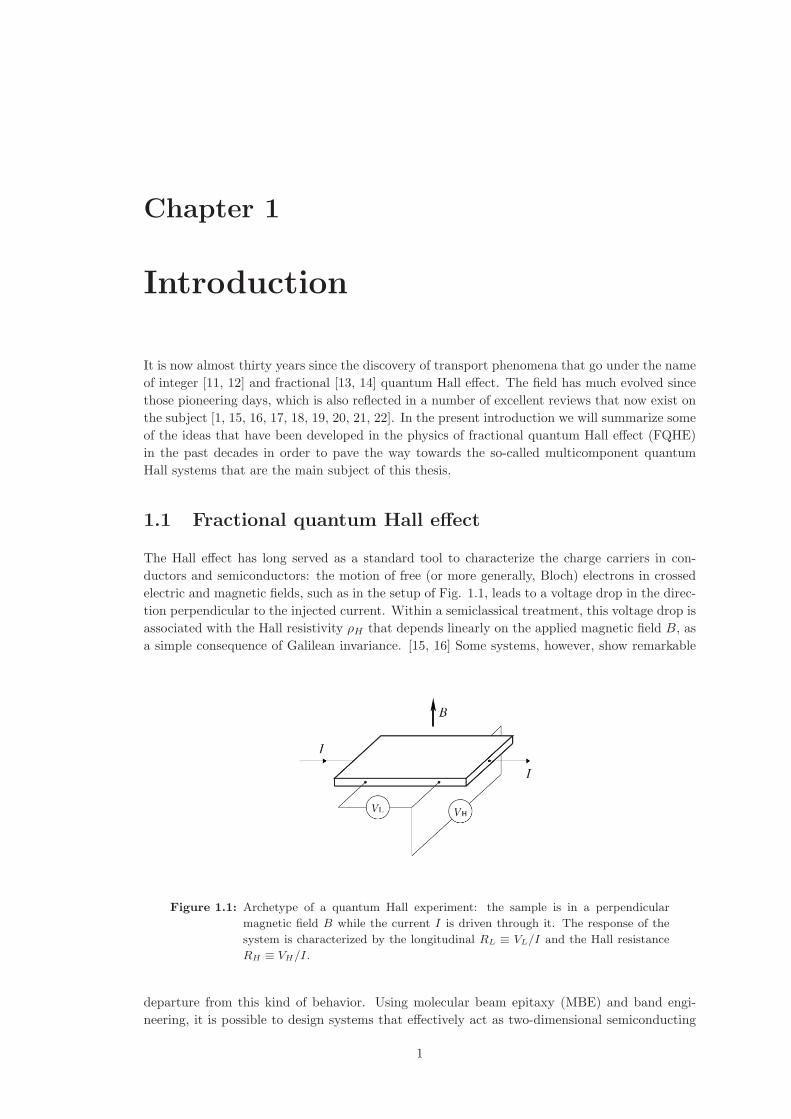
1.1 Archetype of a quantum Hall experiment: the sample is in a perpendicular mag-
netic field B while the current I is driven through it. The response of the system
is characterized by the longitudinal RL ≡ VL/I and the Hall resistance RH ≡ VH/I. 1
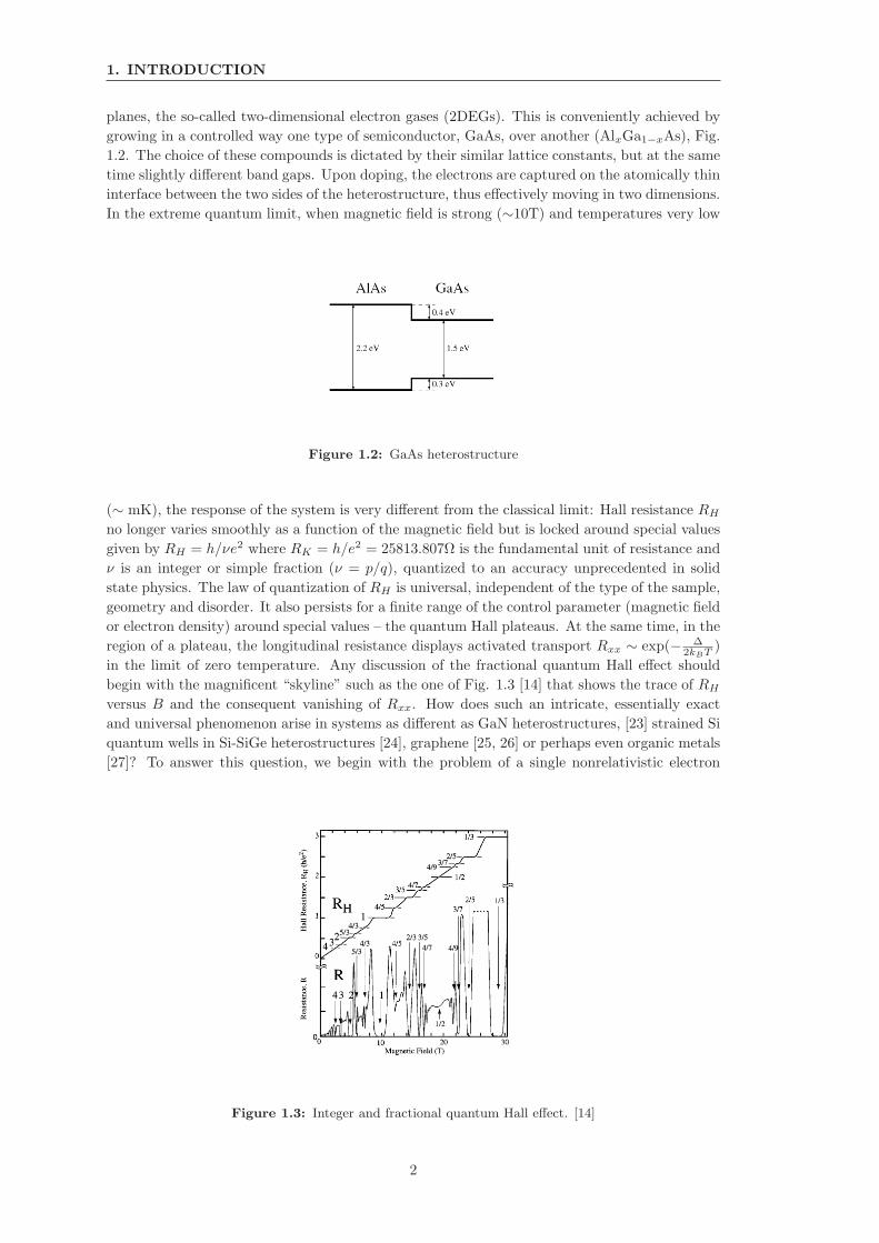
1.2 GaAs heterostructure . . . . . . . . . . . . . . . . . . . . . . . . . . . . . . . . . 2
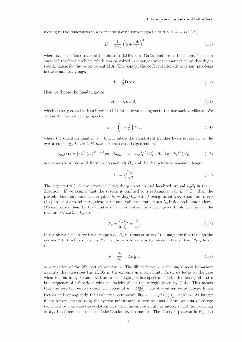
1.3 Integer and fractional quantum Hall effect. [14] . . . . . . . . . . . . . . . . . . . 2
1.4 Quantum well with the two lowest subbands . . . . . . . . . . . . . . . . . . . . . 5
1.5 Chern-Simons transformation to composite bosons . . . . . . . . . . . . . . . . . 7
1.6 FQHE in the second Landau level. [61] . . . . . . . . . . . . . . . . . . . . . . . . 10
1.7 Quantum Hall bilayer: two decoupled layers for large d (left) and the quantum
coherent state for small d (right). . . . . . . . . . . . . . . . . . . . . . . . . . . . 15
1.8 Quantum Hall effect at ν = 1. [88] . . . . . . . . . . . . . . . . . . . . . . . . . . 15
1.9 Tunneling conductance dI/dV as a function of the interlayer bias voltage at total
filling of ν = 1 for several values of d/lB . [93] . . . . . . . . . . . . . . . . . . . . 17
1.10 Rxx and Rxy for the bilayer ν = 1 system at T = 50mK, in the parallel configu-
ration when the currents are flowing in the same direction in both layers (upper
panel) and the counterflow configuration with the two layers contacted individu-
ally (lower panel). The distance between the layers is d/lB = 1.58. [94] . . . . . . 18
1.11 Coulomb drag resistances at T = 30mK in the vicinity of ν = 1 for various d/lB .
[96] . . . . . . . . . . . . . . . . . . . . . . . . . . . . . . . . . . . . . . . . . . . . 19
1.12 Quantum Hall effect at ν = 1/2 in the wide quantum well. [106] . . . . . . . . . 20
1.13 Quantum Hall effect at ν = 1/4 in the presence of parallel magnetic field. [118] . 21
1.14 Quantum Hall effect at ν = 1/2 and ν = 1/4 under density imbalance. [119] . . . 21
1.15 Energy bands of graphene. . . . . . . . . . . . . . . . . . . . . . . . . . . . . . . . 22
2.1 Overlap |〈ΨL|Ψexact〉| between the exact Coulomb state for finite width (ZDS
model) at ν = 1/3 and the Laughlin wave function N = 4 − 12 particles. [133]
Inset: same quantity but in the first excited Landau level i.e. ν = 7/3. . . . . . . 28
2.2 Entanglement spectrum for N = 20 electrons on the sphere, Coulomb interaction
at the filling factor ν = 5/2. The block A consists of NA = 10 electrons and
lA = 19 orbitals, corresponding to the cut [0|0] in Ref. [137]. . . . . . . . . . . . . 29
2.3 Overlap between the exact bilayer state with 553 and 771 states forN = 8 particles
on the sphere. [140] . . . . . . . . . . . . . . . . . . . . . . . . . . . . . . . . . . 30
xi
LIST OF FIGURES
2.4 Low-energy part of the spectrum of the Coulomb interaction on the torus for
N = 10 electrons at ν = 1/3 and the aspect ratio 0.99. Energies are shown
relative to the ground state and, for comparison, we also show the lowest states
of the hard-core V1 potential (2.7). . . . . . . . . . . . . . . . . . . . . . . . . . . 32
2.5 Low-energy part of the spectrum of the three-body Hamiltonian (1.41) on the
torus for N = 12 electrons at ν = 1/2 and aspect ratio 0.99. The three degenerate
zero-energy states are characterized by k = (0, N ′/2), (N ′/2, 0) and (N ′/2, N ′/2). 33
2.6 Energy spectrum of N = 14 electrons on the torus at ν = 1/2 (left) and ν = 5/2
(right), for the aspect ratio of 0.99 . . . . . . . . . . . . . . . . . . . . . . . . . . 34
2.7 Quantum Hall bilayer at the filling factor ν = 1/2 on the torus as a function of
distance d (negligible tunneling). The energy spectrum for N = 8 electrons at the
aspect ratio 0.99 is plotted relative to the ground state at each d and the states
belonging to relevant momentum sectors are highlighted and connected as a guide
to the eye. . . . . . . . . . . . . . . . . . . . . . . . . . . . . . . . . . . . . . . . . 35
3.1 Universality classes of the wave functions Ψ1 (a) and Ψ2 (b), together with their
paired versions, (c) and (d), respectively. . . . . . . . . . . . . . . . . . . . . . . . 40
3.2 Real part of the pseudospin channel density-density correlation [104] and the
Goldstone mode in the case of Ψ1 . . . . . . . . . . . . . . . . . . . . . . . . . . . 45
3.3 Real part of the pseudospin channel density-density correlation [104] in the case
of Ψ2 . . . . . . . . . . . . . . . . . . . . . . . . . . . . . . . . . . . . . . . . . . . 46
3.4 QH bilayer ν = 1 on the torus, N = 16, a/b = 0.99. . . . . . . . . . . . . . . . . . 51
3.5 Ground state energies on the sphere for the QH bilayer at the shift of δ = 1 and 2.
We show the system of N = 8 (which has a filled CF shell in each layer) and the
largest system with N = 16 electrons (without filled CF shells). Similar results
are obtained for other system sizes. . . . . . . . . . . . . . . . . . . . . . . . . . . 52
3.6 Critical bilayer distance dC defined as the crossing point of the ground-state en-
ergies at shifts δ = 1 and δ = 2 on the sphere. Linear extrapolation for N → ∞yields dC ≈ 1.6lB and does not involve the smallest system N = 8 which shows
strong finite-size effects. . . . . . . . . . . . . . . . . . . . . . . . . . . . . . . . . 52
4.1 Overlaps between the exact ground state of the Coulomb bilayer (left panel) and
short range 331 Hamiltonian (right panel) with the 331 state (O331) and the
Pfaffian (OPf), as a function of tunneling ∆SAS . Also shown on the right axis
is the expectation value of the Sx component of pseudospin (for N = 8 system)
which characterizes the two-component to one-component transition. . . . . . . . 58
4.2 Ground state energy for N = 8 and N = 10 electrons on the sphere, d = lB , for
shifts of 2 and 3. . . . . . . . . . . . . . . . . . . . . . . . . . . . . . . . . . . . . 59
4.3 Low-energy part of the spectrum (relative to the ground state) of the short-range
331 (left panel) and the long-range Coulomb Hamiltonian (right panel) for N = 8
electrons on the torus at ν = 1/2 and aspect ratio a/b = 0.97 as a function of
tunneling ∆SAS (right axis). Also shown (left axis) is the overlap with the phases
we identify as the 331 state and the CFL. . . . . . . . . . . . . . . . . . . . . . . 60
4.4 Spectrum of the N = 14 electrons in a single layer at ν = 1/2 interacting with
V +(r) (d = lB), as a function of aspect ratio. We highlight the states with
quantum numbers of the Moore-Read Pfaffian. . . . . . . . . . . . . . . . . . . . 61
xii
LIST OF FIGURES
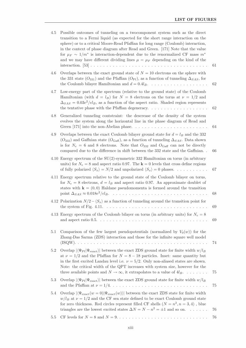
4.5 Possible outcomes of tunneling on a twocomponent system such as the direct
transition to a Fermi liquid (as expected for the short range interaction on the
sphere) or to a critical Moore-Read Pfaffian for long range (Coulomb) interaction,
in the context of phase diagram after Read and Green. [171] Note that the value
for µF ∼ 1/m∗ is interaction-dependent due to the renormalized CF mass m∗
and we may have different dividing lines µ = µF depending on the kind of the
interaction. [53] . . . . . . . . . . . . . . . . . . . . . . . . . . . . . . . . . . . . . 61
4.6 Overlaps between the exact ground state of N = 10 electrons on the sphere with
the 331 state (O331) and the Pfaffian (OPf), as a function of tunneling ∆SAS , for
the Coulomb bilayer Hamiltonian and d = 0.4lB . . . . . . . . . . . . . . . . . . . 62
4.7 Low-energy part of the spectrum (relative to the ground state) of the Coulomb
Hamiltonian (with d = lB) for N = 8 electrons on the torus at ν = 1/2 and
∆SAS = 0.03e2/ǫlB , as a function of the aspect ratio. Shaded region represents
the tentative phase with the Pfaffian degeneracy. . . . . . . . . . . . . . . . . . . 62
4.8 Generalized tunneling contstraint: the descrease of the density of the system
evolves the system along the horizontal line in the phase diagram of Read and
Green [171] into the non-Abelian phase. . . . . . . . . . . . . . . . . . . . . . . . 64
4.9 Overlaps between the exact Coulomb bilayer ground state for d = lB and the 332
(O332) and Gaffnian state (OGaff), as a function of tunneling ∆SAS . Data shown
is for Ne = 6 and 8 electrons. Note that O332 and OGaff can not be directly
compared due to the difference in shift between the 332 state and the Gaffnian. . 66
4.10 Energy spectrum of the SU(2)-symmetric 332 Hamiltonian on torus (in arbitrary
units) for Ne = 8 and aspect ratio 0.97. The k = 0 levels that cross define regions
of fully polarized 〈Sx〉 = N/2 and unpolarized 〈Sx〉 = 0 phases. . . . . . . . . . . 67
4.11 Energy spectrum relative to the ground state of the Coulomb bilayer on torus,
for Ne = 8 electrons, d = lB and aspect ratio 0.97. An approximate doublet of
states with k = (0, 0) Haldane pseudomomenta is formed around the transition
point ∆SAS ≈ 0.018e2/ǫlB . . . . . . . . . . . . . . . . . . . . . . . . . . . . . . . 68
4.12 Polarization N/2−〈Sx〉 as a function of tunneling around the transition point for
the system of Fig. 4.11. . . . . . . . . . . . . . . . . . . . . . . . . . . . . . . . . 69
4.13 Energy spectrum of the Coulomb bilayer on torus (in arbitrary units) for Ne = 8
and aspect ratio 0.5. . . . . . . . . . . . . . . . . . . . . . . . . . . . . . . . . . . 69
5.1 Comparison of the few largest pseudopotentials (normalized by V0(w)) for the
Zhang-Das Sarma (ZDS) interaction and those for the infinite square well model
(ISQW). . . . . . . . . . . . . . . . . . . . . . . . . . . . . . . . . . . . . . . . . . 74
5.2 Overlap |〈ΨPf |Ψexact〉| between the exact ZDS ground state for finite width w/lBat ν = 1/2 and the Pfaffian for N = 8 − 18 particles. Inset: same quantity but
in the first excited Landau level i.e. ν = 5/2. Only non-aliased states are shown.
Note: the critical width of the QPT increases with system size, however for the
three available points and N →∞, it extrapolates to a value of 4lB . . . . . . . . 75
5.3 Overlap |〈ΨPf |Ψexact〉| between the exact ZDS ground state for finite width w/lBand the Pfaffian at ν = 1/4. . . . . . . . . . . . . . . . . . . . . . . . . . . . . . . 75
5.4 Overlap |〈Ψexact(w = 0)|Ψexact(w)〉| between the exact ZDS state for finite width
w/lB at ν = 1/2 and the CF sea state defined to be exact Coulomb ground state
for zero thickness. Red circles represent filled CF shells (N = n2, n = 3, 4) , blue
triangles are the lowest excited states ∆N = N − n2 = ±1 and so on. . . . . . . 76
5.5 CF levels for N = 8 and N = 9. . . . . . . . . . . . . . . . . . . . . . . . . . . . . 76
xiii
LIST OF FIGURES
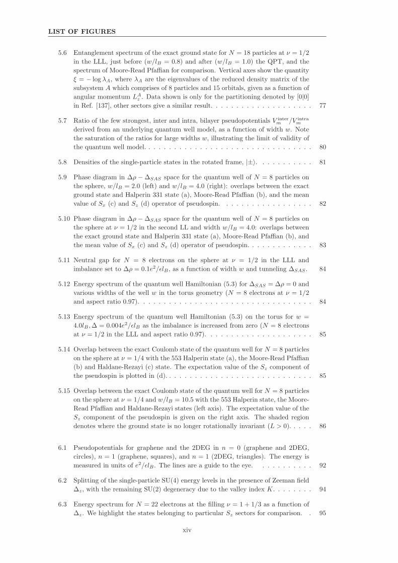
5.6 Entanglement spectrum of the exact ground state for N = 18 particles at ν = 1/2
in the LLL, just before (w/lB = 0.8) and after (w/lB = 1.0) the QPT, and the
spectrum of Moore-Read Pfaffian for comparison. Vertical axes show the quantity
ξ = − log λA, where λA are the eigenvalues of the reduced density matrix of the
subsystem A which comprises of 8 particles and 15 orbitals, given as a function of
angular momentum LAz . Data shown is only for the partitioning denoted by [0|0]
in Ref. [137], other sectors give a similar result. . . . . . . . . . . . . . . . . . . . 77
5.7 Ratio of the few strongest, inter and intra, bilayer pseudopotentials V interm /V intra
m
derived from an underlying quantum well model, as a function of width w. Note
the saturation of the ratios for large widths w, illustrating the limit of validity of
the quantum well model. . . . . . . . . . . . . . . . . . . . . . . . . . . . . . . . . 80
5.8 Densities of the single-particle states in the rotated frame, |±〉. . . . . . . . . . . 81
5.9 Phase diagram in ∆ρ −∆SAS space for the quantum well of N = 8 particles on
the sphere, w/lB = 2.0 (left) and w/lB = 4.0 (right): overlaps between the exact
ground state and Halperin 331 state (a), Moore-Read Pfaffian (b), and the mean
value of Sx (c) and Sz (d) operator of pseudospin. . . . . . . . . . . . . . . . . . 82
5.10 Phase diagram in ∆ρ −∆SAS space for the quantum well of N = 8 particles on
the sphere at ν = 1/2 in the second LL and width w/lB = 4.0: overlaps between
the exact ground state and Halperin 331 state (a), Moore-Read Pfaffian (b), and
the mean value of Sx (c) and Sz (d) operator of pseudospin. . . . . . . . . . . . . 83
5.11 Neutral gap for N = 8 electrons on the sphere at ν = 1/2 in the LLL and
imbalance set to ∆ρ = 0.1e2/ǫlB , as a function of width w and tunneling ∆SAS . 84
5.12 Energy spectrum of the quantum well Hamiltonian (5.3) for ∆SAS = ∆ρ = 0 and
various widths of the well w in the torus geometry (N = 8 electrons at ν = 1/2
and aspect ratio 0.97). . . . . . . . . . . . . . . . . . . . . . . . . . . . . . . . . . 84
5.13 Energy spectrum of the quantum well Hamiltonian (5.3) on the torus for w =
4.0lB ,∆ = 0.004e2/ǫlB as the imbalance is increased from zero (N = 8 electrons
at ν = 1/2 in the LLL and aspect ratio 0.97). . . . . . . . . . . . . . . . . . . . . 85
5.14 Overlap between the exact Coulomb state of the quantum well for N = 8 particles
on the sphere at ν = 1/4 with the 553 Halperin state (a), the Moore-Read Pfaffian
(b) and Haldane-Rezayi (c) state. The expectation value of the Sz component of
the pseudospin is plotted in (d). . . . . . . . . . . . . . . . . . . . . . . . . . . . . 85
5.15 Overlap between the exact Coulomb state of the quantum well for N = 8 particles
on the sphere at ν = 1/4 and w/lB = 10.5 with the 553 Halperin state, the Moore-
Read Pfaffian and Haldane-Rezayi states (left axis). The expectation value of the
Sz component of the pseudospin is given on the right axis. The shaded region
denotes where the ground state is no longer rotationally invariant (L > 0). . . . . 86
6.1 Pseudopotentials for graphene and the 2DEG in n = 0 (graphene and 2DEG,
circles), n = 1 (graphene, squares), and n = 1 (2DEG, triangles). The energy is
measured in units of e2/ǫlB . The lines are a guide to the eye. . . . . . . . . . . 92
6.2 Splitting of the single-particle SU(4) energy levels in the presence of Zeeman field
∆z, with the remaining SU(2) degeneracy due to the valley index K. . . . . . . . 94
6.3 Energy spectrum for N = 22 electrons at the filling ν = 1 + 1/3 as a function of
∆z. We highlight the states belonging to particular Sz sectors for comparison. . 95
xiv
LIST OF FIGURES
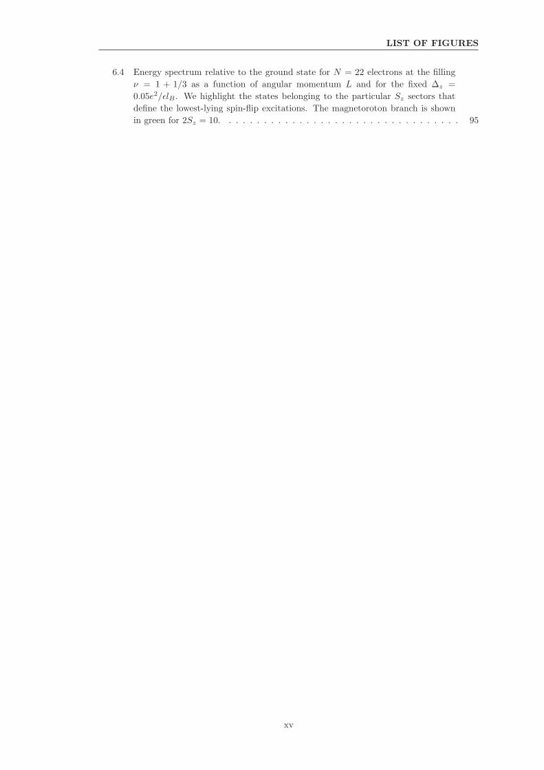
6.4 Energy spectrum relative to the ground state for N = 22 electrons at the filling
ν = 1 + 1/3 as a function of angular momentum L and for the fixed ∆z =
0.05e2/ǫlB . We highlight the states belonging to the particular Sz sectors that
define the lowest-lying spin-flip excitations. The magnetoroton branch is shown
in green for 2Sz = 10. . . . . . . . . . . . . . . . . . . . . . . . . . . . . . . . . . 95
xv

LIST OF FIGURES
xvi
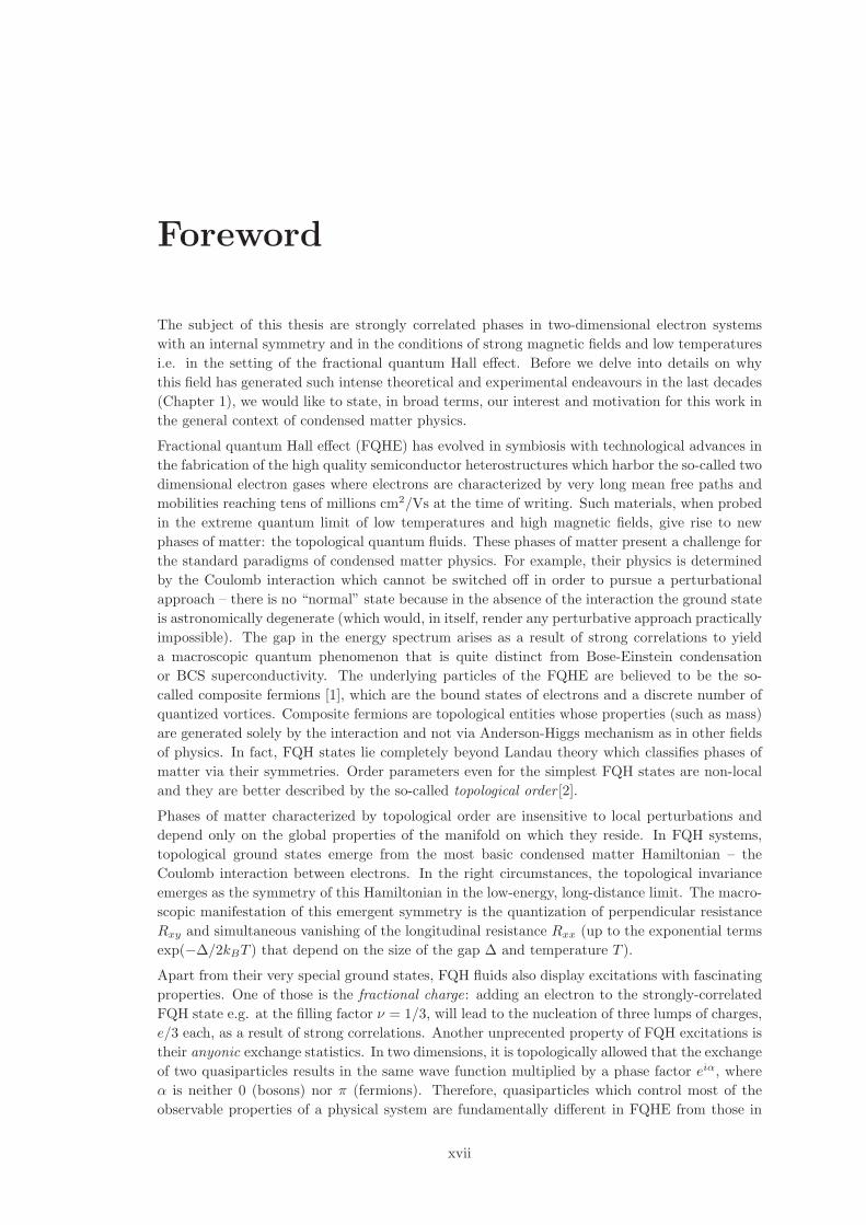
Foreword
The subject of this thesis are strongly correlated phases in two-dimensional electron systems
with an internal symmetry and in the conditions of strong magnetic fields and low temperatures
i.e. in the setting of the fractional quantum Hall effect. Before we delve into details on why
this field has generated such intense theoretical and experimental endeavours in the last decades
(Chapter 1), we would like to state, in broad terms, our interest and motivation for this work in
the general context of condensed matter physics.
Fractional quantum Hall effect (FQHE) has evolved in symbiosis with technological advances in
the fabrication of the high quality semiconductor heterostructures which harbor the so-called two
dimensional electron gases where electrons are characterized by very long mean free paths and
mobilities reaching tens of millions cm2/Vs at the time of writing. Such materials, when probed
in the extreme quantum limit of low temperatures and high magnetic fields, give rise to new
phases of matter: the topological quantum fluids. These phases of matter present a challenge for
the standard paradigms of condensed matter physics. For example, their physics is determined
by the Coulomb interaction which cannot be switched off in order to pursue a perturbational
approach – there is no “normal” state because in the absence of the interaction the ground state
is astronomically degenerate (which would, in itself, render any perturbative approach practically
impossible). The gap in the energy spectrum arises as a result of strong correlations to yield
a macroscopic quantum phenomenon that is quite distinct from Bose-Einstein condensation
or BCS superconductivity. The underlying particles of the FQHE are believed to be the so-
called composite fermions [1], which are the bound states of electrons and a discrete number of
quantized vortices. Composite fermions are topological entities whose properties (such as mass)
are generated solely by the interaction and not via Anderson-Higgs mechanism as in other fields
of physics. In fact, FQH states lie completely beyond Landau theory which classifies phases of
matter via their symmetries. Order parameters even for the simplest FQH states are non-local
and they are better described by the so-called topological order [2].
Phases of matter characterized by topological order are insensitive to local perturbations and
depend only on the global properties of the manifold on which they reside. In FQH systems,
topological ground states emerge from the most basic condensed matter Hamiltonian – the
Coulomb interaction between electrons. In the right circumstances, the topological invariance
emerges as the symmetry of this Hamiltonian in the low-energy, long-distance limit. The macro-
scopic manifestation of this emergent symmetry is the quantization of perpendicular resistance
Rxy and simultaneous vanishing of the longitudinal resistance Rxx (up to the exponential terms
exp(−∆/2kBT ) that depend on the size of the gap ∆ and temperature T ).
Apart from their very special ground states, FQH fluids also display excitations with fascinating
properties. One of those is the fractional charge: adding an electron to the strongly-correlated
FQH state e.g. at the filling factor ν = 1/3, will lead to the nucleation of three lumps of charges,
e/3 each, as a result of strong correlations. Another unprecented property of FQH excitations is
their anyonic exchange statistics. In two dimensions, it is topologically allowed that the exchange
of two quasiparticles results in the same wave function multiplied by a phase factor eiα, where
α is neither 0 (bosons) nor π (fermions). Therefore, quasiparticles which control most of the
observable properties of a physical system are fundamentally different in FQHE from those in
xvii
0. FOREWORD
more common condensed matter systems such as metals, magnets or liquid helium, where they
are either bosons or fermions. In fact, FQHE allows for even more exotic kinds of quasiparticles
with the so-called non-Abelian exchange statistics. Suppose that a system has a g-degenerate
ground-state multiplet Ψa, a = 1, . . . g. This could be the so-called Moore-Read Pfaffian state
at ν = 5/2. [3] Exchanging two quasiparticles can lead to the initial state Ψa being mapped
to a linear combination of some other states in the multiplet, so that the exchange operation is
represented not by a phase, but by a matrix Ψa → MabΨb. A subsequent exchange would lead
(in general) to a different matrix N and, because M and N do not necessarily commute, we
refer to this process as the non-Abelian braiding of quasiparticles. If we have in mind the FQH
state where the ground-state multiplet is topologically protected by the system’s excitation
gap, we can use the entangled state of the quasiparticles as a basis for a qubit and perform
quantum operations by braiding the quasiparticles. This idea is inherently free of decoherence
problems and could be a platform for fault-tolerant topological quantum computation [4, 5],
the potential practical importance of FQHE. Although recent proposals for TQC (see [6] and
references therein) seem more in favor of p-wave superconductors and topological insulators [7, 8],
FQH systems remain one of the most important arenas for investigating exotic excitations and
establishing non-Abelian statistics in nature.
If spin or some other internal quantum number of the electrons is not completely frozen out,
we deal with the multicomponent FQH systems. [9] These include electrons with spin, bilayer
structures where layer index assumes the role of the spin (Chapter 3 and 4), wide quantum wells
(Chapter 5), or graphene (Chapter 6), where valley and spin indices combine into an SU(4)-spin.
The most important experimental ramification to date has been the observation of Bose-Einstein
condensation of excitons in the ν = 1 quantum Hall bilayer. [10] The exciton in a quantum Hall
bilayer is formed by an electron in one layer and a hole opposite to it in the other layer. The
idea of exciton condensation has a long tradition, but it has proved elusive in the era before the
QH bilayer experiments. The importance of multicomponent degrees of freedom lies in that they
allow the formation of FQH states at filling factors which are more difficult to describe or do not
exist in polarized systems, such as ν = 1/2. They are also related to the non-Abelian states – the
latter can be viewed as the (anti)symmetrized versions of the former. This connection between
non-Abelian and multicomponent states and the quantum phase transitions between them is a
fundamental, open problem. Although the non-Abelian states in multicomponent systems are
likely to be very fragile and not directly useful for applications such as topological quantum
computation, the study of the multicomponent systems provides insight also into the polarized
states as the two of them share many characteristics in the low-energy description. This is one
of the goals of this thesis.
xviii
Chapter 1
Introduction
It is now almost thirty years since the discovery of transport phenomena that go under the name
of integer [11, 12] and fractional [13, 14] quantum Hall effect. The field has much evolved since
those pioneering days, which is also reflected in a number of excellent reviews that now exist on
the subject [1, 15, 16, 17, 18, 19, 20, 21, 22]. In the present introduction we will summarize some
of the ideas that have been developed in the physics of fractional quantum Hall effect (FQHE)
in the past decades in order to pave the way towards the so-called multicomponent quantum
Hall systems that are the main subject of this thesis.
1.1 Fractional quantum Hall effect
The Hall effect has long served as a standard tool to characterize the charge carriers in con-
ductors and semiconductors: the motion of free (or more generally, Bloch) electrons in crossed
electric and magnetic fields, such as in the setup of Fig. 1.1, leads to a voltage drop in the direc-
tion perpendicular to the injected current. Within a semiclassical treatment, this voltage drop is
associated with the Hall resistivity ρH that depends linearly on the applied magnetic field B, as
a simple consequence of Galilean invariance. [15, 16] Some systems, however, show remarkable
Figure 1.1: Archetype of a quantum Hall experiment: the sample is in a perpendicular
magnetic field B while the current I is driven through it. The response of the
system is characterized by the longitudinal RL ≡ VL/I and the Hall resistance
RH ≡ VH/I.
departure from this kind of behavior. Using molecular beam epitaxy (MBE) and band engi-
neering, it is possible to design systems that effectively act as two-dimensional semiconducting
1
1. INTRODUCTION
planes, the so-called two-dimensional electron gases (2DEGs). This is conveniently achieved by
growing in a controlled way one type of semiconductor, GaAs, over another (AlxGa1−xAs), Fig.
1.2. The choice of these compounds is dictated by their similar lattice constants, but at the same
time slightly different band gaps. Upon doping, the electrons are captured on the atomically thin
interface between the two sides of the heterostructure, thus effectively moving in two dimensions.
In the extreme quantum limit, when magnetic field is strong (∼10T) and temperatures very low
Figure 1.2: GaAs heterostructure
(∼ mK), the response of the system is very different from the classical limit: Hall resistance RH
no longer varies smoothly as a function of the magnetic field but is locked around special values
given by RH = h/νe2 where RK = h/e2 = 25813.807Ω is the fundamental unit of resistance and
ν is an integer or simple fraction (ν = p/q), quantized to an accuracy unprecedented in solid
state physics. The law of quantization of RH is universal, independent of the type of the sample,
geometry and disorder. It also persists for a finite range of the control parameter (magnetic field
or electron density) around special values – the quantum Hall plateaus. At the same time, in the
region of a plateau, the longitudinal resistance displays activated transport Rxx ∼ exp(− ∆2kBT )
in the limit of zero temperature. Any discussion of the fractional quantum Hall effect should
begin with the magnificent “skyline” such as the one of Fig. 1.3 [14] that shows the trace of RH
versus B and the consequent vanishing of Rxx. How does such an intricate, essentially exact
and universal phenomenon arise in systems as different as GaN heterostructures, [23] strained Si
quantum wells in Si-SiGe heterostructures [24], graphene [25, 26] or perhaps even organic metals
[27]? To answer this question, we begin with the problem of a single nonrelativistic electron
Figure 1.3: Integer and fractional quantum Hall effect. [14]
2
1.1 Fractional quantum Hall effect
moving in two dimensions in a perpendicular uniform magnetic field ∇×A = Bz [28],
H =1
2mb
(
p +eA
c
)2
(1.1)
where mb is the band mass of the electron (0.067me in GaAs) and −e is the charge. This is a
standard textbook problem which can be solved in a gauge-invariant manner or by choosing a
specific gauge for the vector potential A. The popular choice for rotationally invariant problems
is the symmetric gauge,
A =1
2B× r. (1.2)
Here we choose the Landau gauge,
A = (0, Bx, 0), (1.3)
which directly casts the Hamiltonian (1.1) into a form analogous to the harmonic oscillator. We
obtain the discrete energy spectrum
En =
(
n+1
2
)
~ωc, (1.4)
where the quantum number n = 0, 1, ... labels the equidistant Landau levels separated by the
cyclotron energy ~ωc = ~eB/mbc. The associated eigenvectors
φn,X(r) =[
π22n(n!)2]−1/4
exp[
ikyy − (x− kyl2B)2/2l2B
]
Hn
[
(x− kyl2B)/lB
]
(1.5)
are expressed in terms of Hermite polynomials Hn and the characteristic magnetic length
lB =
√
~c
eB. (1.6)
The eigenstates (1.5) are extended along the y-direction and localized around kyl2B in the x-
direction. If we assume that the system is confined to a rectangular cell Lx × Ly, then the
periodic boundary condition requires ky = 2πj/Ly, with j being an integer. Since the energy
(1.4) does not depend on ky, there is a number of degenerate states Ns inside each Landau level.
We enumerate them by the number of allowed values for j that give orbitals localized in the
interval 0 < kyl2B < Lx i.e.
Ns =LxLy
2πl2B=
Φ
Φ0. (1.7)
In the above formula we have reexpressed Ns in terms of ratio of the magnetic flux through the
system Φ to the flux quantum, Φ0 = hc/e, which leads us to the definition of the filling factor
ν,
ν =N
Ns= 2πl2Bn, (1.8)
as a function of the 2D electron density n. The filling factor ν is the single most important
quantity that describes the 2DEG in the extreme quantum limit. First, we focus on the case
when ν is an integer number. Due to the single particle spectrum (1.4), the density of states
is a sequence of δ-functions with the weight Ns at the energies given by (1.4). This means
that the zero-temperature chemical potential µ =(
∂E∂N
)
Bhas discontinuities at integer filling
factors and consequently the isothermal compressibility κ−1 = ρ2(
dµdρ
)
Tvanishes. At integer
filling factors, compressing the system infinitesimally requires thus a finite amount of energy
(sufficient to overcome the cyclotron gap). The incompressibility at integer ν and the vanishing
of Rxx is a direct consequence of the Landau level structure. The observed plateaus in Rxy can
3
1. INTRODUCTION
be accounted for by disorder in real samples. Disorder modifies the spectrum in the manner
that degenerate LL states broaden into bands. The single particle states near the unperturbed
energies (1.4) form bands of extended states. [29] The extended bands are separated by localized
states which do not contribute to the transport (this is called “mobility gap”) and thus the Hall
plateaus may form.
Looking back at Fig. 1.3 we notice many cases with ν < 1 that seem to yield the same experi-
mental phenomenology as those with ν integer. If so, let us focus on the case ν < 1 for the time
being and ask what is the cause of incompressibility here. A simple combinatorial calculation
of how many ways there are for placing N electrons on Ns > N sites (N being a macroscopic
number) yields a vast ground state degeneracy. As it was realized and proved in the early 1980s,
it is the Coulomb repulsion between electrons that lifts this degeneracy and singles out a unique
incompressible ground state for particular values of ν that is identified by the presence of a
plateau in transport measurements and, more generally, the minimum in longitudinal resistance.
These incompressible states have many intriguing properties that we will describe in more detail
in the following Sections. All these properties can in principle be derived from the following
master Hamiltonian of a quantum Hall system of N electrons in magnetic field B:
H =∑
i
Hsingle(ri) +e2
ǫ
∑
i<j
1
|ri − rj |+∑
i
U(ri) + gµB · S. (1.9)
The first term represents the single particle Hamiltonians (1.1), followed by two-body Coulomb
interaction and one-body interaction with the positive background charges and the disorder,∑
i U(ri). The last term describes the coupling of total spin S to the magnetic field. Hamiltonian
(1.9) has the following typical energy scales for a GaAs heterostructure (Fig. 1.2). The single-
particle energy scale is that of the cyclotron energy,
~ωc ≈ 20B [T] K, (1.10)
the Coulomb energy scales as
e2
ǫlB≈ 50
√
B [T] K, (1.11)
the Zeeman splitting is
2gµBB · S ≈ 0.3B [T] K, (1.12)
with the unit of length being lB ≈ 25/√
B [T] nm (1.6). For theoretical discussions, it is often
convenient to work in “God’s units” for the FQHE:
lB = 1,e2
ǫlB= 1, (1.13)
and those will be implicitly assumed in this thesis unless stated otherwise. Usually, a number
of approximations is made on the Hamiltonian (1.9). We will switch off disorder because we are
not interested in the physics of the plateaus, but only in the formation of incompressible states.
Furthermore, we assume that the cyclotron energy (1.10) is large enough so that we do not need
to explicitly treat more than a single Landau level. This assumption is actually incorrect in
the experiments but most calculations would be impossible or very difficult to do without it.
Furthermore, it is often customary to assume that the electron’s wave function is a δ-function in
the perpendicular direction, so that the dynamics is strictly two-dimensional. This is of course
just an approximation but there is no obvious way how the finite-width correction should be
implemented. For a heterostructure such as the one in Fig. 1.2, the self-consistent potential
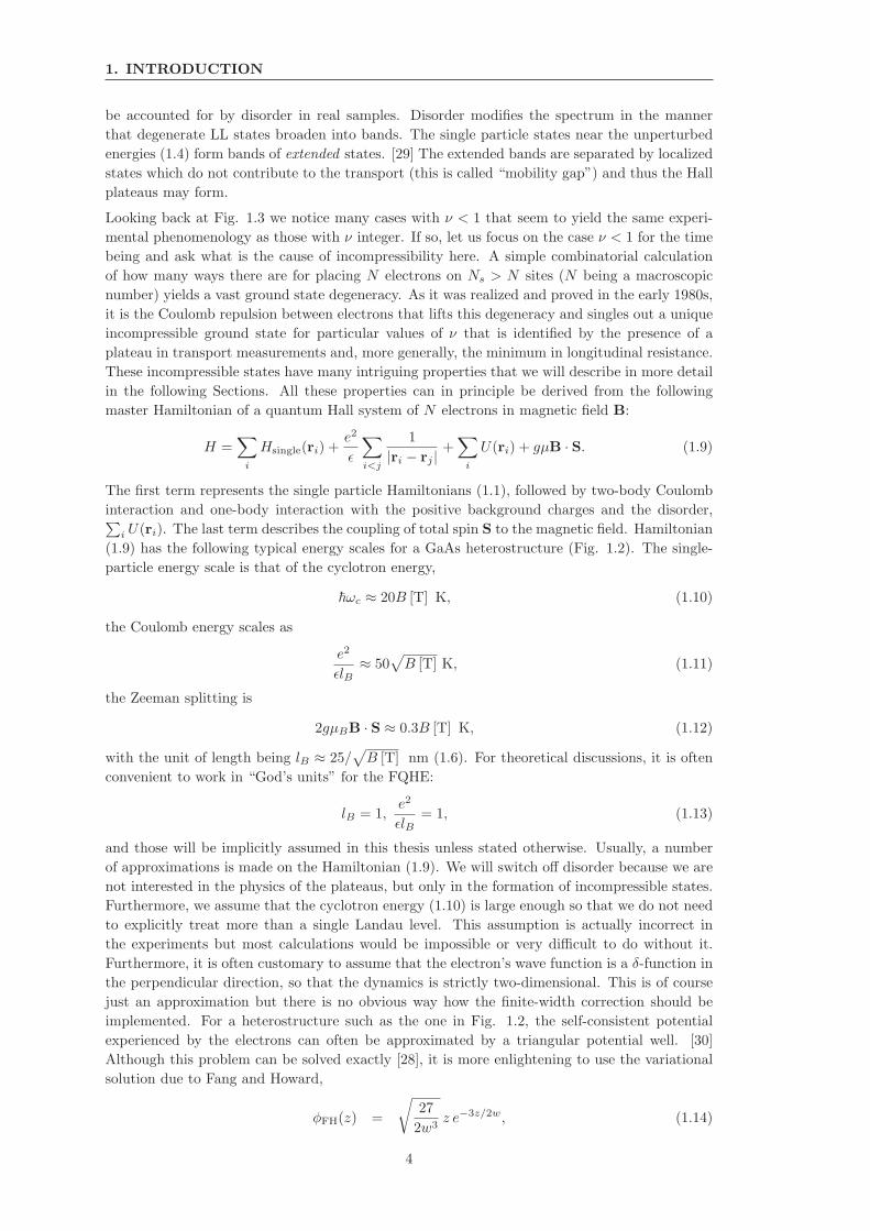
experienced by the electrons can often be approximated by a triangular potential well. [30]
Although this problem can be solved exactly [28], it is more enlightening to use the variational
solution due to Fang and Howard,
φFH(z) =
√
27
2w3z e−3z/2w, (1.14)
4
1.2 Polarized electrons in the lowest Landau level
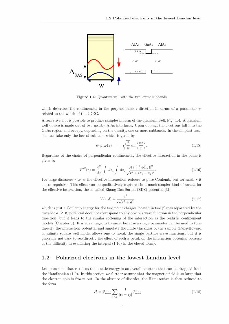
Figure 1.4: Quantum well with the two lowest subbands
which describes the confinement in the perpendicular z-direction in terms of a parameter w
related to the width of the 2DEG.
Alternatively, it is possible to produce samples in form of the quantum well, Fig. 1.4. A quantum
well device is made out of two nearby AlAs interfaces. Upon doping, the electrons fall into the
GaAs region and occupy, depending on the density, one or more subbands. In the simplest case,
one can take only the lowest subband which is given by
φISQW(z) =
√
2
wsin(πz
w
)
. (1.15)
Regardless of the choice of perpendicular confinement, the effective interaction in the plane is
given by
V eff(r) =e2
ǫlB
∫
dz1
∫
dz2|φ(z1)|2|φ(z2)|2√
r2 + (z1 − z2)2. (1.16)
For large distances r ≫ w the effective interaction reduces to pure Coulomb, but for small r it
is less repulsive. This effect can be qualitatively captured in a much simpler kind of ansatz for
the effective interaction, the so-called Zhang-Das Sarma (ZDS) potential [31]
V (r, d) =e2
ǫ√r2 + d2
, (1.17)
which is just a Coulomb energy for the two point charges located in two planes separated by the
distance d. ZDS potential does not correspond to any obvious wave function in the perpendicular
direction, but it leads to the similar softening of the interaction as the realistic confinement
models (Chapter 5). It is advantageous to use it because a single parameter can be used to tune
directly the interaction potential and simulate the finite thickness of the sample (Fang-Howard
or infinite square well model allows one to tweak the single particle wave functions, but it is
generally not easy to see directly the effect of such a tweak on the interaction potential because
of the difficulty in evaluating the integral (1.16) in the closed form).
1.2 Polarized electrons in the lowest Landau level
Let us assume that ν < 1 so the kinetic energy is an overall constant that can be dropped from
the Hamiltonian (1.9). In this section we further assume that the magnetic field is so large that
the electron spin is frozen out. In the absence of disorder, the Hamiltonian is then reduced to
the form
H = PLLL
∑
i<j
1
|ri − rj |PLLL (1.18)
5
1. INTRODUCTION
i.e. it contains nothing but the interaction (explicitly projected to the LLL by the operator
PLLL ). This is why the quantum Hall effect is referred to as the paradigm of strongly correlated
systems. In the case of a partially filled nth LL, one may separate the “low-energy” degrees of
freedom, which consist of intra-LL excitations, from the “high-energy” inter-LL excitations. In
the absence of disorder, all states within the partially filled LL have the same kinetic energy such
that intra-LL excitations may be described by considering only electron-electron interactions,
Hn =1
2
∑
q
v(q)ρn(−q)ρn(q), (1.19)
where v(q) = 2πe2/ǫq is the 2D Fourier-transformed Coulomb interaction potential. The Fourier
components ρn(q) of the density operator are constructed solely from states within the n-th LL.
Eq. (1.19) is a Fourier-image of Eq. (1.18) and is valid for 2DEG as well as for other systems
such as graphene in the magnetic field (Sec. 1.5.5) if the density operators are appropriately
modified (Chapter 6).
1.2.1 Laughlin’s wave function
Since it contains only the interaction, Hamiltonian (1.18) is notoriously difficult to solve because
there is no obvious normal state to use as the starting point for the perturbation theory and
essentially one has to make an educated guess at what the ground state could possibly be. This
was first done by Laughlin [32] who proposed the following wave function for the states at filling
factors ν = 1/m,m− odd integer,
ΨL =∏
i<j
(zi − zj)m exp
(
−∑
k
|zk|2/4)
, (1.20)
zj = xj + iyj is the complex coordinate of an electron in the plane (lB = 1) and we will drop
the universal Gaussian factor from now on. To understand this wave function, one should use
the symmetric gauge (1.2) which yields LLL single particle wave functions that are analytic
functions of z and have definite angular momentum l, φl(z) ∼ zl exp(−|z|2/4). Using these
wave functions and the Jastrow-type variational ansatz known from the physics of liquid He,
Laughlin constructed the many-body wave function which captures the correct physics at the
filling factor ν = 1/3 which was observed at the time. Namely, he showed that ν = 1/m states
are incompressible fluids with a uniform density. The latter property is nontrivial to establish in
the disk geometry and a formal mapping to a 2D plasma is required [33] (in the finite systems,
on the contrary, it is very simple to verify this property numerically, see Chapter 2). Using a
flux insertion argument, Laughlin also demonstrated that incompressibility at a fractional filling
factor implies the existence of fractionally charge excitations [33] that were eventually observed
in shot noise experiments. [34, 35] An interesting consequence of the fractional charge of the
quasiparticles is their fractional mutual statistics. Based on general arguments [33, 36] (see also
Sec. 1.3.2), it is possible to write a wave function for the two quasiholes at u and v
Ψ2qhL = (u− v)1/m
∏
i,j
(zi − u)(zj − v)ΨL(z) exp[
−(|u|2 + |v|2)/4m]
. (1.21)
If we perform an exchange operation on the quasiholes u and v, we notice that the phase of the
wave function changes by π/m, instead of the usual π or 2π (for fermions and bosons, respec-
tively). In doing so, we assume that the wave function Ψ2qhL is properly normalized. [37, 38, 39]
Thus, the quasiholes (and similarly, quasiparticles) in the Laughlin state obey anyonic (Abelian)
statistics. [40] In Sec. 1.3 we will see even more exotic possibilities for the mutual statistics of
quasiparticles that are possibly brought by strong correlations in FQHE. The experiments that
directly address the statistics of quasiparticles are largely based on interferometry principles and
have so far proved difficult to interpret.
6
1.2 Polarized electrons in the lowest Landau level
Immediate support of Laughlin’s theory came however from exact diagonalization studies [41, 42]
which, among other things, identified the interaction that produces Laughlin’s wave function as
a unique zero energy ground state with the smallest angular momentum:
V (r) = V∇2δ(r), (1.22)
V being a positive constant that controls the value of the gap. Properly taking care of the short-
range correlations makes the Laughlin wave function an excellent description of the generic
Coulomb ground state, for fermions as well as for bosons. [43, 44] It was further shown that
the Laughlin state possesses a low-energy branch of collective modes called magneto-rotons [45]
(in analogy with rotons in liquid helium) and established that there is a hidden, so-called off-
diagonal long-range order [46] in the Laughlin ground state. The latter insight was a starting
point for the development of the effective Chern-Simons field theories for the fractional quantum
Hall states (see the following Section).
To close this brief overview of the Laughlin states, we stress that the Laughlin states are to this
day the first experimentally known examples of a new kind of matter which possesses topological
order. [2] The topological phase of matter is the one canonically characterized by the presence
of gap in the excitation spectrum, fractional quantum numbers (such as the quasiparticle charge
in the present case) and with a ground state degeneracy on topologically nontrivial manifolds,
[2, 47] although some of these may not be the necessary requirements. Not all of these properties
are easily proven even for the Laughlin state (e.g. there is no rigorous proof that the Laughlin
state is gapped in thermodynamic limit), but there is plenty of numerical evidence and the
overall consensus is that this is indeed the case.
1.2.2 Effective field theories
Zhang, Hansson and Kivelson have shown, building on an earlier work by Girvin and MacDonald
[46], that applying a singular gauge transformation to the electron coordinates can map them
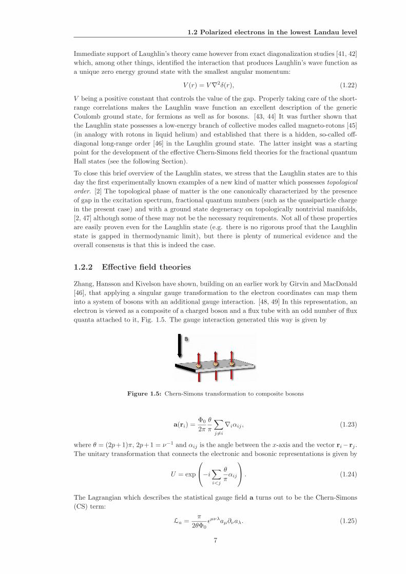
into a system of bosons with an additional gauge interaction. [48, 49] In this representation, an
electron is viewed as a composite of a charged boson and a flux tube with an odd number of flux
quanta attached to it, Fig. 1.5. The gauge interaction generated this way is given by
Figure 1.5: Chern-Simons transformation to composite bosons
a(ri) =Φ0
2π
θ
π
∑
j 6=i
∇iαij , (1.23)
where θ = (2p+1)π, 2p+1 = ν−1 and αij is the angle between the x-axis and the vector ri−rj .
The unitary transformation that connects the electronic and bosonic representations is given by
U = exp
−i∑
i<j
θ
παij
. (1.24)
The Lagrangian which describes the statistical gauge field a turns out to be the Chern-Simons
(CS) term:
La =π
2θΦ0ǫµνλaµ∂νaλ. (1.25)
7
1. INTRODUCTION
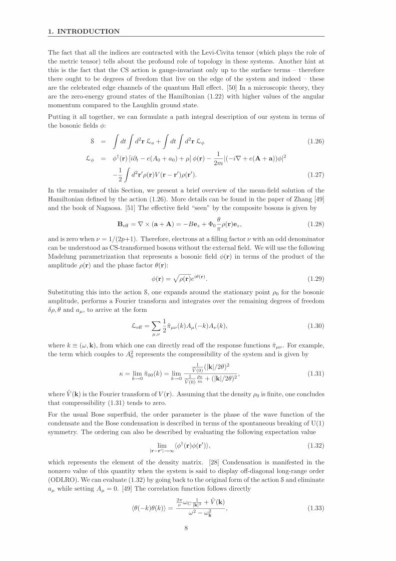
The fact that all the indices are contracted with the Levi-Civita tensor (which plays the role of
the metric tensor) tells about the profound role of topology in these systems. Another hint at
this is the fact that the CS action is gauge-invariant only up to the surface terms – therefore
there ought to be degrees of freedom that live on the edge of the system and indeed – these
are the celebrated edge channels of the quantum Hall effect. [50] In a microscopic theory, they
are the zero-energy ground states of the Hamiltonian (1.22) with higher values of the angular
momentum compared to the Laughlin ground state.
Putting it all together, we can formulate a path integral description of our system in terms of
the bosonic fields φ:
S =
∫
dt
∫
d2r La +
∫
dt
∫
d2r Lφ (1.26)
Lφ = φ†(r) [i∂t − e(A0 + a0) + µ]φ(r)− 1
2m|(−i∇+ e(A + a))φ|2
−1
2
∫
d2r′ρ(r)V (r− r′)ρ(r′). (1.27)
In the remainder of this Section, we present a brief overview of the mean-field solution of the
Hamiltonian defined by the action (1.26). More details can be found in the paper of Zhang [49]
and the book of Nagaosa. [51] The effective field “seen” by the composite bosons is given by
Beff = ∇× (a + A) = −Bez + Φ0θ
πρ(r)ez, (1.28)
and is zero when ν = 1/(2p+1). Therefore, electrons at a filling factor ν with an odd denominator
can be understood as CS-transformed bosons without the external field. We will use the following
Madelung parametrization that represents a bosonic field φ(r) in terms of the product of the
amplitude ρ(r) and the phase factor θ(r):
φ(r) =√
ρ(r)eiθ(r). (1.29)
Substituting this into the action S, one expands around the stationary point ρ0 for the bosonic
amplitude, performs a Fourier transform and integrates over the remaining degrees of freedom
δρ, θ and aµ, to arrive at the form
Leff =∑
µ,ν
1
2πµν(k)Aµ(−k)Aν(k), (1.30)
where k ≡ (ω,k), from which one can directly read off the response functions πµν . For example,
the term which couples to A20 represents the compressibility of the system and is given by
κ = limk→0
π00(k) = limk→0
1V (0)
(|k|/2θ)21
V (0)
ρ0
m + (|k|/2θ)2 , (1.31)
where V (k) is the Fourier transform of V (r). Assuming that the density ρ0 is finite, one concludes
that compressibility (1.31) tends to zero.
For the usual Bose superfluid, the order parameter is the phase of the wave function of the
condensate and the Bose condensation is described in terms of the spontaneous breaking of U(1)
symmetry. The ordering can also be described by evaluating the following expectation value
lim|r−r′|→∞
〈φ†(r)φ(r′)〉, (1.32)
which represents the element of the density matrix. [28] Condensation is manifested in the
nonzero value of this quantity when the system is said to display off-diagonal long-range order
(ODLRO). We can evaluate (1.32) by going back to the original form of the action S and eliminate
aµ while setting Aµ = 0. [49] The correlation function follows directly
〈θ(−k)θ(k)〉 =
2πν ωC
1|k|2 + V (k)
ω2 − ω2k
, (1.33)
8

1.2 Polarized electrons in the lowest Landau level
where ω2k = ω2
C + ρ0
m |k|2V (k) and ωC = 2πρ0
mν . The static correlation function is asymptotically
〈θ(−k)θ(k)〉 = −i∫
dω
2π〈θ(−k)θ(k)〉 = − 1
2ν
2π
|k|2 + o (1/|k|) . (1.34)
Going back to real space, (1.32) becomes
lim|r−r′|→∞
〈φ†(r)φ(r′)〉 = ρ0〈eiθ(r)−iθ(r′)〉 ≈ ρ0e〈θ(r)θ(r′)〉
∝ ρ0|r− r′|−1/2ν , (1.35)
where in the first line we expanded the exponential and used Wick’s theorem. The obtained
ODLRO (1.35) is algebraic and does not depend on the interaction V .
Magneto-roton excitations are described by topological vortices of this theory and, neglecting
their contribution to the ground state, one can derive Laughlin’s wave function directly as
the ground state description [49, 51] (see also Chapter 3). However, it has proved difficult to
generalize the composite boson theory for the non-Laughlin fractions and also to translate it into
a microscopic theory which can be tested numerically (some effort in this direction was made in
[52]). In Chapter 3 we will use a generalization of this kind of theory to describe the phases of
the quantum Hall bilayer at ν = 1.
1.2.3 Composite fermions
A compelling generalization of Laughlin’s theory exists for most of the polarized FQH states
observed in the LLL due to Jain. [1] This theory can be introduced following a similar trans-
formation as the one outlined in the previous Section, the only difference being that electrons
are now capturing an even number θ = 2p of flux quanta. This means that they preserve their
fermionic statistics and therefore are called composite fermions. When it happens that compos-
ite fermions have just the right number of available (residual) flux quanta left for them to fill
the integer number of ν∗ = n LLs, one can readily write down trial wave functions to describe
their ground state (the image of this ground state in terms of the original electrons will be a
complicated, strongly correlated state). Since the CF ground state is unique being the integer
QH state, the incompressibility follows immediately. There is an additional subtlety in that
electrons are not capturing flux tubes but rather vortices, as it is explained in great detail in
Ref. [1]. Here we quote the expression for the wave functions that describe the filling factors
ν = n2pn±1 :
Ψν= n2pn±1
= PLLLΦ±n
∏
i<j
(zi − zj)2p, (1.36)
where Φ±n is the Slater determinant for n filled CF LLs which are called Λ levels (with a sign
depending on the direction of the residual magnetic field). Notice that unless n = 1, Φ±n
has non-analytic components because it is not a LLL function. Therefore, a projection operator
PLLL is required to explicitly project the whole expression to the LLL. The wave functions (1.36)
are remarkable test wave functions as they do not contain any variational parameters, yet they
show impressive agreement with the complicated ground states of realistic systems in numerical
calculations. The formation of CFs is a nonperturbative outcome of the strongly correlated
system, but similarly to the true quasiparticles known in other areas of physics, CFs are mostly
weakly interacting. For polarized electrons, the topological properties of their excitations are
Abelian.
1.2.4 Compressible state ν = 1/2
A striking feature in Fig. 1.3 is the absence of a plateau at ν = 1/2. Halperin, Lee and Read [53]
made a remarkable proposal for the state at ν = 1/2 as a compressible Fermi liquid state of CFs
9
1. INTRODUCTION
(CFL) that experience zero residual magnetic field. They calculated the response functions in
the long-wavelength effective theory and some of these features were verified in surface acoustic
wave experiments. [54] On the other hand, Rezayi and Read [55] have formulated a microscopic
wave function for such a compressible state at ν = 1/2,
ΨRR = PLLLF(z, z)∏
i<j
(zi − zj)2, (1.37)
where multiplication with a Slater determinant of free waves F ≡ det[
eiki·rj]
is necessary to
ensure a fermionic wave function. The relevance of (1.37) has been numerically demonstrated.
[55]
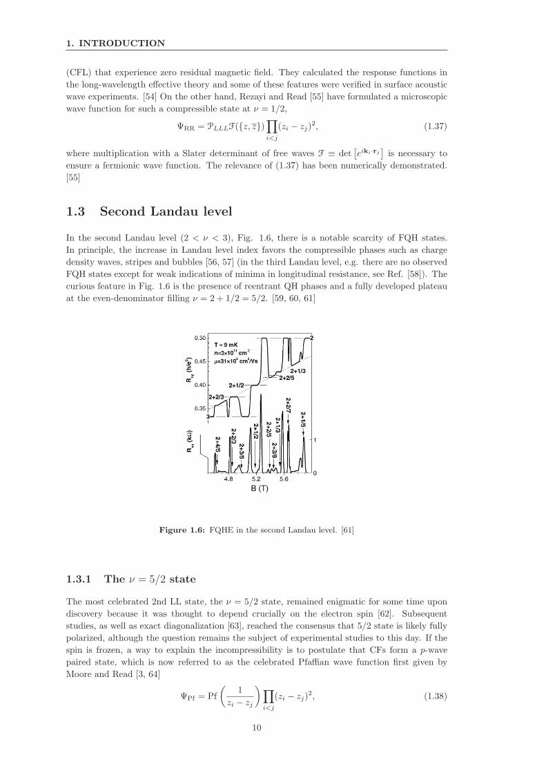
1.3 Second Landau level
In the second Landau level (2 < ν < 3), Fig. 1.6, there is a notable scarcity of FQH states.
In principle, the increase in Landau level index favors the compressible phases such as charge
density waves, stripes and bubbles [56, 57] (in the third Landau level, e.g. there are no observed
FQH states except for weak indications of minima in longitudinal resistance, see Ref. [58]). The
curious feature in Fig. 1.6 is the presence of reentrant QH phases and a fully developed plateau
at the even-denominator filling ν = 2 + 1/2 = 5/2. [59, 60, 61]
Figure 1.6: FQHE in the second Landau level. [61]
1.3.1 The ν = 5/2 state
The most celebrated 2nd LL state, the ν = 5/2 state, remained enigmatic for some time upon
discovery because it was thought to depend crucially on the electron spin [62]. Subsequent
studies, as well as exact diagonalization [63], reached the consensus that 5/2 state is likely fully
polarized, although the question remains the subject of experimental studies to this day. If the
spin is frozen, a way to explain the incompressibility is to postulate that CFs form a p-wave
paired state, which is now referred to as the celebrated Pfaffian wave function first given by
Moore and Read [3, 64]
ΨPf = Pf
(
1
zi − zj
)
∏
i<j
(zi − zj)2, (1.38)
10
1.3 Second Landau level
where “Pf” stands for the Pfaffian
Pf Mij =1
2N/2(N/2)!
∑
σ∈SN
sgnσ
N/2∏
k=1
Mσ(2k−1)σ(2k)
for an N ×N antisymmetric matrix whose elements are Mij ; SN is the group of permutations of
N objects. The Pfaffian factor guarantees the correct exchange symmetry of the wave function
and acts only in the so-called neutral sector of the wave function, without affecting the filling
factor which is fixed by the Jastrow factor. The latter is referred to as the charge part of the
wave function. The Pfaffian wave function has a much richer spectrum of excitations than the
Laughlin states, its excitations carry charge e/4 and obey the so-called non-Abelian statistics.
[3, 65] If 2n quasiholes are introduced above the ground state, it can be shown they give rise to
2n−1 linearly independent states. [65] If we set N = 2 electrons and look for the wave functions
that describe the four quasiholes above the ground state, we obtain two independent states that
span the basis proposed by Nayak and Wilczek [66]:
Ψ4qh0 =
(η13η24)1/4
(1 +√
1− x)1/2
(
Ψ(13)(24) +√
1− xΨ(14)(23)
)
(1.39)
Ψ4qh1/2 =
(η13η24)1/4
(1−√
1− x)1/2
(
Ψ(13)(24) −√
1− xΨ(14)(23)
)
(1.40)
where η’s denote the positions of the quasiholes, x = η12η34
η13η24and η12 ≡ η1 − η2 etc. We have
defined Ψ(12)(34) = Ψν=1/2L (z1 − z2)−1 × [(z1 − η1)(z1 − η2)(z2 − η3)(z2 − η4) + (z1 ↔ z2)] and
we assume that all of the quasihole wave functions are normalized [37, 38, 39]. If we focus on
the limit |x| ≪ 1, we have approximately
Ψ4qh0 = 2−1/2(η13η24)
1/4(
Ψ(13)(24) + Ψ(14)(23)
)
Ψ4qh1/2 = 2−1/2(η13η24)
1/4(
Ψ(13)(24) −Ψ(14)(23)
)
It is clear that the exchange e.g. of 1 and 3 leads only to the multiplication by a phase factor.
However, the interchange of 2 and 3 gives a rotation in the space Ψ4qh0 ,Ψ4qh
1/2. Therefore, the
states Ψ4qh0 and Ψ4qh
1/2 can be used as a basis for a qubit. Braiding of the qubit states can be used
to perform quantum operations which are protected from decoherence effects due to the FQH
gap. This is the motivation for using FQH states in topological quantum computation schemes.
Non-Abelian properties of ν = 5/2 excitations have so far been numerically demonstrated [67]
and experiments to test this are under way. [68] Several groups have reported the observation of
e/4 fractional charges at 5/2 filling. [69, 70] The key to establishing the non-Abelian statistics
in theory, apart from the ground state wave function (1.38), is to identify the Hamiltonian which
produces the given wave function as its densest zero-energy ground state, similar to (1.22). In the
case of the Pfaffian, this is the Hamiltonian which has no penalty for two electrons approaching
each other, but forbids the clustering of three electrons:
H3b = −∑
i<j<k
Sijk
[
∇4i∇2
jδ(ri − rj)δ(rj − rk)]
, (1.41)
where Sijk is the symmetrizer. Numerical studies of realistic systems [71] have shown that
Pfaffian is a very good trial wave function for the ground state, especially if the interaction
is modified with respect to the pure Coulomb by adding some short-range potential of the
kind (1.22), and also by particle-hole symmetrizing the Moore-Read wave function. Note that
the Moore-Read wave function, being the ground state of 3-body interaction (1.41), is not
particle-hole symmetric. The state obtained via particle-hole conjugation of the Pfaffian wave
function (1.38) is called anti-Pfaffian [72, 73] and has recently received much attention as a
viable candidate for the description of the 5/2 state. [74, 75]
11
1. INTRODUCTION
1.3.2 Conformal field theory approach
In this Section we outline the method of conformal field theory (CFT) [76] that historically lead
to the construction of the trial wave function (1.38). Conformal field theories have successfully
been used to describe two-dimensional statistical mechanics models in the vicinity of critical
points, when the correlation length diverges and there is an emergent conformal symmetry.
[77] In two dimensions, this emergent symmetry is sufficient to derive critical exponents. FQH
systems, on the other hand, are not critical but CFT can nonetheless be used due to the following
observation (see [78] for a review of CFT in this context).
Take a free boson theory in 1+1-dimensional Euclidean spacetime, with the correlator given by
〈φ(z)φ(z′)〉 = − ln(z − z′). (1.42)
Further defining the normal-ordered vertex operators Vα(z) =: eiαφ(z) :, with the help of Wick’s
theorem, their correlators evaluate to
⟨
∏
i
Vαi(zi)
⟩
=∏
i<j
(zi − zj)αiαj , (1.43)
if the neutrality condition is assumed∑
i αi = 0 (or else the correlator identically vanishes). If we
choose αi =√m, we obtain precisely the polynomial part of the Laughlin wave function, (1.20).
The Gaussian factor can similarly be constructed assuming a uniform background charge. We
also get wave functions for n quasiholes (u1, ..., un) for free if we insert V1/√
m(u1)...V1/√
m(un)
into the correlator (1.43). Quasielectron wave functions can also be constructed with some effort.
[79]
Thus, CFT correlators have been shown to be a legitimate tool to produce candidate wave
functions for FQH states [3, 80, 81, 82, 83] if the latter can be verified by independent means.
In particular, Moore and Read [3] in their seminal work combined the chiral boson theory with
the Majorana fermion, described by correlator 〈χ(z)χ(z′)〉 = 1/(z− z′), to arrive at the Pfaffian
(1.38)
⟨
∏
i
χ(zi)ei√
(2)φ(zi)
⟩
. (1.44)
More generally, instead of a Majorana fermion, it is possible to use the Zk parafermion algebra
to construct generalizations of a Pfaffian paired state for the fillings ν = k/(k+2). [84] These are
the states which allow for clustering of k particles and forbid (k + 1)-particle clusters, with the
excitations having non-Abelian statistics. Case k = 2 is the Pfaffian and there are indications
that k = 3 is also physically relevant, being the particle-hole conjugate of the second LL ν = 2/5
state observed in the experiments. [61] Braiding of the quasiparticles in states with k = 3 and
k > 4 can be used to perform fault-tolerant quantum computation and hence presents an exciting
venue for further research. [5]
All of the previously described CFTs are known as unitary. There have been attempts [82] that
produce wave functions out of nonunitary CFTs, such as the so-called “Gaffnian” wave function
which is related to the so-called M(5, 3) minimal model [76] and describes a possible state at
the filling factor ν = 2/5. In numerical studies, Gaffnian appears as a serious contender for the
description of 2/5 state (the role shared by Jain’s CF state), but on general grounds [39, 85]
it is expected to describe a critical point rather than a stable incompressible phase. Both
Gaffnian and Jain 2/5 state have an underlying multicomponent structure which we explain in
the following Section. Deeper understanding of the role of nonunitary CFTs and related FQH
states is the subject of on-going research.
12
1.4 Multicomponent quantum Hall systems
1.4 Multicomponent quantum Hall systems
In this thesis, we understand the term “multicomponent” to loosely refer to FQH systems with
an internal degree of freedom. This degree of freedom is most naturally provided by electron
spin when the magnetic field is not too strong to completely freeze out its dynamics. Looking at
the relative interaction strengths (1.10, 1.11, 1.12), we see that the Zeeman splitting is less than
the Coulomb or cyclotron energy in the accessible B range and we need to explicitly take it into
account. This was first suggested by Halperin [86] who also wrote down a generalization of the
Laughlin wave function for these systems. Halperin’s wave functions in the case of an ordinary
SU(2) spin are defined by dividing the electrons into two species (with ↑ and ↓ spin projection)
and introducing correlations among them, in a manner of Laughlin’s wave function (1.20), so
each electron “sees” the same number of flux quanta because they are indistinguishable particles:
ΨHm1,m2,n(z↑j , z
↓j ) =
N↑∏
k<l
(
z↑k − z↑l
)m1
N↓∏
k<l
(
z↓k − z↓l
)m2
N↑∏
k=1
N↓∏
l=1
(
z↑k − z↓l
)n
. (1.45)
We have dropped the Gaussian factors for simplicity and the set of the exponents (m1,m2, n)
characterize the wave function. The requirement that each electron “sees” the same number of
flux quanta translates into the condition m1(N↑ − 1) + nN↓ = m2(N↓ − 1) + nN↑. With the
help of the total number of electrons N = N↑ + N↓, the filling factor that this wave function
describes is
ν = ν↑ + ν↓ =m1 +m2 − 2n
m1m2 − n2, (1.46)
except when m1m2 − n2 = 0. The physical realization of the last condition is the Laughlin
ferromagnetic wave function m1 = m2 = n which does not fix the relative number of ↑ and ↓particles. There is also an additional constraint that (1.45) needs to satisfy if it is to be a proper
trial wave function for the spinful system: it must be the eigenstate of the total spin operator
S2, which places constraints on the values of m1,m2, n. However, as we will see below, this
requirement can be lifted in certain situations where the SU(2) symmetry is not fully respected
by the Hamiltonian.
It is possible to write down also the generalization of Halperin wave functions for systems with
an SU(K) internal symmetry. These are expected to described quantized states in K-component
systems such as graphene (Sec. 1.5.5). In graphene, a valley and spin degree of freedom (for a
certain range of interaction strengths) combine into an effective SU(4) degree of freedom (K = 4).
Generalized Halperin wave functions are given by
ψSU(K)m1,...,mK ;nij
(
z(1)j1, z
(2)j2, ..., z
(K)jK
)
= ΨLm1,...,mK
× Ψinternij
(1.47)
which consists of a product of Laughlin wave functions
ΨLm1,...,mK
=K∏
j=1
Nj∏
kj<lj
(
z(j)kj− z(j)
lj
)mj
for each of the components and a term
Ψinternij
=
K∏
i<j
Ni∏
ki
Nj∏
kj
(
z(i)ki− z(j)
kj
)nij
that takes into account the correlations between particles of different components. Many prop-
erties of these wave functions for general K can be worked out using the usual arguments such
as flux counting and plasma analogy to assess their stability and identify those that are viable
candidates to describe physical systems. [87]
Besides the intrinsic electron spin, multicomponent GaAs QH systems can be easily fabricated
in the experiment in the form of wide quantum wells (Sec. 1.4.1) or bilayers (Sec. 1.4.2), where
13
1. INTRODUCTION
the subband or layer index plays the role of the spin-like degree of freedom. In what follows
we will introduce these systems and provide an overview of the physical phenomena that are
studied in this thesis (Sec. 1.5).
1.4.1 Wide quantum wells
In Section 1.1 we introduced the quantum well structure (Fig. 1.4). It consists of two nearby
AlAs interfaces, resulting in a semiconductor quantum well. Upon doping, the electrons fall into
the GaAs region and occupy, depending on the density, one or more subbands. The width of
the well w is usually between 15 and 50nm, while the depth of the well is on the order of 0.4eV,
which is often much larger than other energy scales and therefore can be assumed infinite. The
splitting between the subbands, ∆SAS , scales as 1/w2, but it is expected to be renormalized in
each sample, so it is convenient to think of it as a free parameter. What may happen is that the
lowest two subbands are relevant for the low-energy description of the electrons, as indicated on
the left side of Fig. 1.4, while we can discard the rest of the higher energy levels. The reason why
we can sometimes keep only the two lowest subbands and discard the rest of the energy levels
is subtle because, in a single particle picture, the gap between the lowest and the first excited
subband is not very different from the one between the first excited and the second excited
subband. In Chapter 5 we will quantify the range of validity of the two-subband approximation
on the mean-field level. This calculation will show that, at least for some moderate values of
the well width, we can restrict the dynamics to the lowest two subbands. For the infinite square
well, the lowest two levels happen to be the sine functions, labeled S and A:
φS≡↑(z) =
√
2
wsin(πz
w
)
, φA≡↓(z) =
√
2
wsin
(
2πz
w
)
. (1.48)
The two-subband model is often a very good approximation in the experiments and provides a
useful mapping of the quantum well system to a multicomponent description (see Chapter 5).
The internal symmetry in this case is provided by the subband quantum number instead of the
usual z-projection of spin. Therefore, we expect that FQH states observed in samples with the
geometry of a quantum well can be described by Halperin wave functions (1.45). Note, however,
that φS and φA have different symmetry regarding the reflection with respect to the center of
the well z = w/2: the former is symmetric, while the latter is antisymmetric (it possesses a node
at the center of the well). This implies that the problem does not have full SU(2) symmetry and
therefore we are not obliged to require the ΨHm1,m2,n to be an eigenstate of S2.
1.4.2 Quantum Hall bilayer
Bilayer semiconductor structure consists of two quantum wells grown by MBE and spatially
separated by an insulating barrier that is on the same order of magnitude as the width of each
of the wells, Fig. 1.7. The key parameter that describes this system is d/lB , the ratio of center-
to-center distance d to the magnetic length lB . Applying gate voltage changes the electron
density in each layer, which in turns changes the effective magnetic length and therefore also
d/lB . Note that besides the top/bottom gates which control the electron density (and are not
in direct contact with the 2DEG), separate Ohmic contacts that are annealed onto the sample
can be used to probe electronic transport. Theoretically we describe the quantum Hall bilayer
imagining that there are two groups of electrons situated in the ↑ and ↓ layer. Electrons within
the same layer interact with the unscreened Coulomb interaction V intra(r), whereas electrons in
different groups repel each other by a slightly weaker interaction,V inter(r)
V intra(r) = e2/ǫr, V inter(r) = e2/ǫ√
r2 + d2. (1.49)
Additional energy scale is set by the tunneling between the layers. However, it is possible to
fabricate bilayer systems which have negligible tunneling and interesting quantum mechanical
14
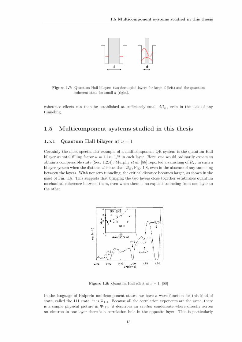
1.5 Multicomponent systems studied in this thesis
Figure 1.7: Quantum Hall bilayer: two decoupled layers for large d (left) and the quantum
coherent state for small d (right).
coherence effects can then be established at sufficiently small d/lB , even in the lack of any
tunneling.
1.5 Multicomponent systems studied in this thesis
1.5.1 Quantum Hall bilayer at ν = 1
Certainly the most spectacular example of a multicomponent QH system is the quantum Hall
bilayer at total filling factor ν = 1 i.e. 1/2 in each layer. Here, one would ordinarily expect to
obtain a compressible state (Sec. 1.2.4). Murphy et al. [88] reported a vanishing of Rxx in such a
bilayer system when the distance d is less than 2lB , Fig. 1.8, even in the absence of any tunneling
between the layers. With nonzero tunneling, the critical distance becomes larger, as shown in the
inset of Fig. 1.8. This suggests that bringing the two layers close together establishes quantum
mechanical coherence between them, even when there is no explicit tunneling from one layer to
the other.
Figure 1.8: Quantum Hall effect at ν = 1. [88]
In the language of Halperin multicomponent states, we have a wave function for this kind of
state, called the 111 state: it is Ψ111. Because all the correlation exponents are the same, there
is a simple physical picture in Ψ111: it describes an exciton condensate where directly across
an electron in one layer there is a correlation hole in the opposite layer. This is particularly
15
1. INTRODUCTION
transparent in the wave function proposed by Fertig [89], Ψ111 =∏
m1√2
(
c†m↑ + c†m↓
)
|0〉, which
can be understood as “grand canonical” generalization of Ψ111. The numbers of particles in ↑and ↓ layer are not sharp in Ψ111 (i.e. their difference N↑ − N↓ fluctuates, while the sum is
fixed), but they are both individually conserved in Ψ111. Because the excitons are neutral, the
bilayer for d = 0 can also be understood as a composite boson condensate [90] (Sec. 1.2.2).
In d → 0 limit the SU(2) pseudospin rotation symmetry makes the bilayer system equivalent
to the Heisenberg problem, in which spins can rotate freely in three dimensions. At finite d,
the intralayer repulsion is stronger than interlayer repulsion. If the pseudospins would order
in the z-direction, all of the electrons would be in a single layer and the capacitive charging
energy would be large. That would lead to an “easy-plane” anisotropy in which the pseudospins
prefer to order in x − y plane and the symmetry is reduced to U(1) (see Ref. [91] for a quick
introduction to the physics of spin and pseudospin in quantum Hall systems). This is made
explicit by comparing the ground state of the easy-plane ferromagnet [9, 92]
ΨXY =∏
m
1√2
(
c†m↑ + eiφc†m↓
)
|0〉. (1.50)
to Ψ111. The phase φ represents a global phase difference between ↑ and ↓ particles and in-
terpolates between the symmetric (φ = 0) and antisymmetric (φ = π) superposition. Similar
to the BCS wave function of a superconductor, the phase φ is fixed, but the particle number
fluctuates. To be precise, the total number of particles is fixed, but the particle number differ-
ence between the layers is indefinite. However, contrary to the Cooper-pair order parameter, the
order parameter here
〈ψ†↑(r)ψ↓(r)〉 ∼ eiφ(r)
is charge-neutral and can condense even in high magnetic fields.
In the absence of tunneling between the layers, the Hamiltonian of the system should not depend
on the phase φ, but it may nonetheless depend on its gradient
HXY =ρs
2
∫
d2r |∇φ|2, (1.51)
ρs being the pseudospin stiffness which is typically about 0.5K [92] and represents the energy
cost of twisting the pseudospins out of their perfect alignment. This low-energy description is
known as the Berezinskii-Kosterlitz-Thouless (BKT) model. [51] It displays a topological phase
transition at finite temperatures on the order of ρs, driven by proliferation of vortices. The
transition occurs when the vortices in the phase field φ become unbound as a result of entropy
gain (although their interaction energy grows logarithmically with distance). In the context
of QH bilayer, vortices are known as merons and they carry both charge and vorticity. [92]
The broken U(1) symmetry in the bilayer at ν = 1 has received a stunning confirmation in
the experiments of Spielman et al. [93] who studied interlayer transport as a function of bias
voltage, Fig. 1.9. At large d/lB the interlayer conductance is strongly supressed. As the layers
are nearly decoupled for large d/lB , there is an energy penalty for an electron that tunnels from
one correlated state into the other as the latter needs to be reorganized to accomodate the extra
electrons. This is not so when d/lB is below 1.8. As seen in Fig. 1.9, a sharp resonance develops
at zero bias voltage which can be accounted for by the excitonic condensation in the 111 state.
Opposite to each electron there is now a hole and it is energetically advantageous for an electron
to tunnel. The effect is reminiscent of the Josephson effect, although strictly speaking the two
“weak links” in this case are parts of the same quantum state.
Further experimental support for the picture of an excitonic superfluid forming in the ν = 1
bilayer came from the so-called counterflow experiments. As the excitons are charge neutral
and hence do not carry a net current, their presence can be detected in a configuration in which
the injected currents in the two layers are equal in magnitude but flow in opposite directions,
Fig. 1.10. The fundamental charge carriers can be electrons [94] or holes. [95] As seen in
16
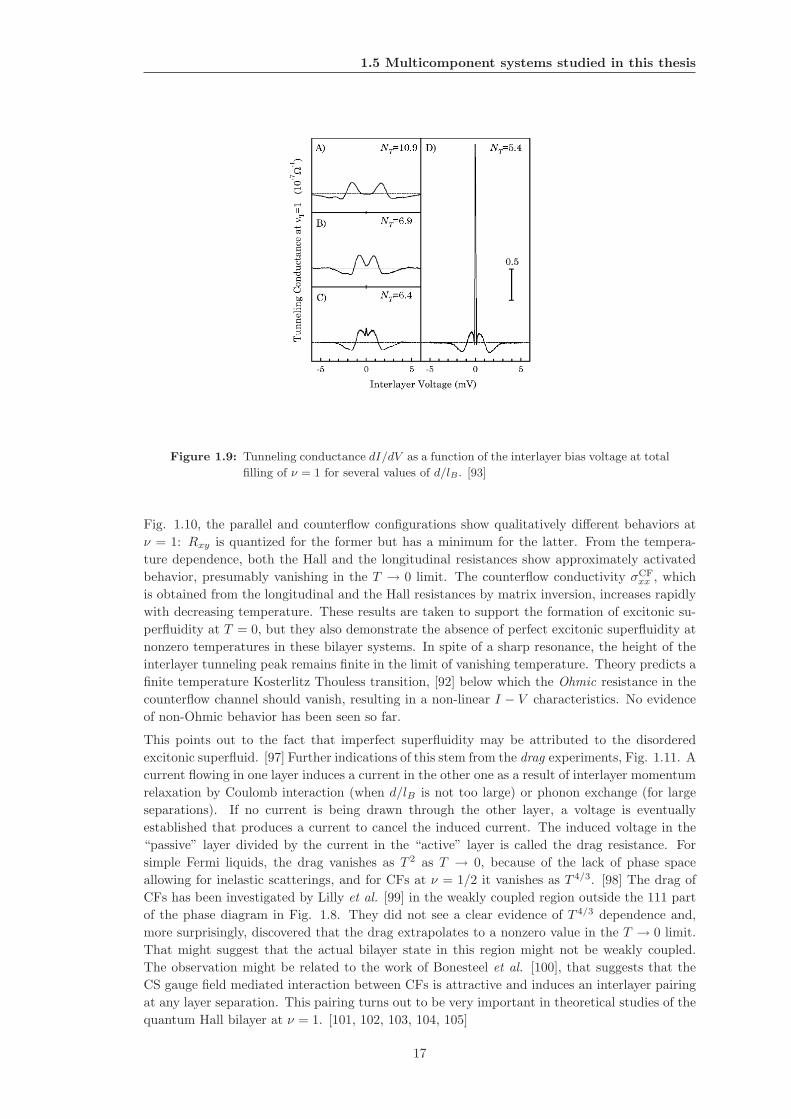
1.5 Multicomponent systems studied in this thesis
Figure 1.9: Tunneling conductance dI/dV as a function of the interlayer bias voltage at total
filling of ν = 1 for several values of d/lB . [93]
Fig. 1.10, the parallel and counterflow configurations show qualitatively different behaviors at
ν = 1: Rxy is quantized for the former but has a minimum for the latter. From the tempera-
ture dependence, both the Hall and the longitudinal resistances show approximately activated
behavior, presumably vanishing in the T → 0 limit. The counterflow conductivity σCFxx , which
is obtained from the longitudinal and the Hall resistances by matrix inversion, increases rapidly
with decreasing temperature. These results are taken to support the formation of excitonic su-
perfluidity at T = 0, but they also demonstrate the absence of perfect excitonic superfluidity at
nonzero temperatures in these bilayer systems. In spite of a sharp resonance, the height of the
interlayer tunneling peak remains finite in the limit of vanishing temperature. Theory predicts a
finite temperature Kosterlitz Thouless transition, [92] below which the Ohmic resistance in the
counterflow channel should vanish, resulting in a non-linear I − V characteristics. No evidence
of non-Ohmic behavior has been seen so far.
This points out to the fact that imperfect superfluidity may be attributed to the disordered
excitonic superfluid. [97] Further indications of this stem from the drag experiments, Fig. 1.11. A
current flowing in one layer induces a current in the other one as a result of interlayer momentum
relaxation by Coulomb interaction (when d/lB is not too large) or phonon exchange (for large
separations). If no current is being drawn through the other layer, a voltage is eventually
established that produces a current to cancel the induced current. The induced voltage in the
“passive” layer divided by the current in the “active” layer is called the drag resistance. For
simple Fermi liquids, the drag vanishes as T 2 as T → 0, because of the lack of phase space
allowing for inelastic scatterings, and for CFs at ν = 1/2 it vanishes as T 4/3. [98] The drag of
CFs has been investigated by Lilly et al. [99] in the weakly coupled region outside the 111 part
of the phase diagram in Fig. 1.8. They did not see a clear evidence of T 4/3 dependence and,
more surprisingly, discovered that the drag extrapolates to a nonzero value in the T → 0 limit.
That might suggest that the actual bilayer state in this region might not be weakly coupled.
The observation might be related to the work of Bonesteel et al. [100], that suggests that the
CS gauge field mediated interaction between CFs is attractive and induces an interlayer pairing
at any layer separation. This pairing turns out to be very important in theoretical studies of the
quantum Hall bilayer at ν = 1. [101, 102, 103, 104, 105]
17
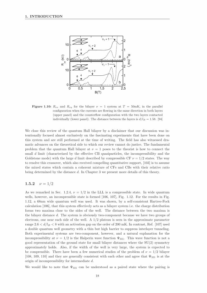
1. INTRODUCTION
Figure 1.10: Rxx and Rxy for the bilayer ν = 1 system at T = 50mK, in the parallel
configuration when the currents are flowing in the same direction in both layers
(upper panel) and the counterflow configuration with the two layers contacted
individually (lower panel). The distance between the layers is d/lB = 1.58. [94]
We close this review of the quantum Hall bilayer by a disclaimer that our discussion was in-
tentionally focused almost exclusively on the fascinating experiments that have been done on
this system and are still performed at the time of writing. The field has also witnessed dra-
matic advances on the theoretical side to which our review cannot do justice. The fundamental
problem that the quantum Hall bilayer at ν = 1 poses to the theorist is how to connect the
small d limit (characterized by the effective CB quasiparticles, the incompressibility and the
Goldstone mode) with the large d limit described by compressible CF ν = 1/2 states. The way
to resolve this crossover, which also received compelling quantitative support, [103] is to assume
the mixed states which contain a coherent mixture of CFs and CBs with their relative ratio
being determined by the distance d. In Chapter 3 we present more details of this theory.
1.5.2 ν = 1/2
As we remarked in Sec. 1.2.4, ν = 1/2 in the LLL is a compressible state. In wide quantum
wells, however, an incompressible state is formed [106, 107], Fig. 1.12. For the results in Fig.
1.12, a 68nm wide quantum well was used. It was shown, by a self-consistent Hartree-Fock
calculation [106], that this system effectively acts as a bilayer system i.e. the charge distribution
forms two maxima close to the sides of the well. The distance between the two maxima is
the bilayer distance d. The system is obviously two-component because we have two groups of
electrons, one near each side of the well. A 1/2 plateau is seen in the approximate parameter
range 2.6 < d/lB < 8 with an activation gap on the order of 200 mK. In contrast, Ref. [107] used
a double quantum well geometry with a thin but high barrier to suppress interlayer tunneling.
Both experimental systems are two-component, however, and a natural explanation for the
incompressibility at ν = 1/2 is the Halperin wave function Ψ331. This wave function is not a
good representation of the ground state for small bilayer distances where the SU(2) symmetry
approximately holds. Also, if the width of the well is very large, the system is expected to
be compressible. There have been a few numerical studies of the problem of ν = 1/2 bilayer
[108, 109, 110] and they are generally consistent with each other and agree that Ψ331 is at the
origin of incompressibility for intermediate d.
We would like to note that Ψ331 can be understood as a paired state where the pairing is
18
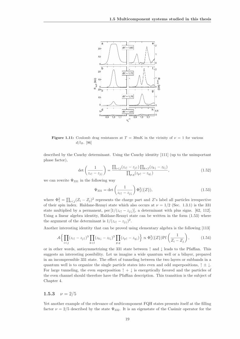
1.5 Multicomponent systems studied in this thesis
Figure 1.11: Coulomb drag resistances at T = 30mK in the vicinity of ν = 1 for various
d/lB . [96]
described by the Cauchy determinant. Using the Cauchy identity [111] (up to the unimportant
phase factor),
det
(
1
zi↑ − zj↓
)
=
∏
i<j(zi↑ − zj↑)∏
k<l(zk↓ − zl↓)∏
p,q(zp↑ − zq↓), (1.52)
we can rewrite Ψ331 in the following way
Ψ331 = det
(
1
zi↑ − zj↓
)
Φ21(Z), (1.53)
where Φ21 =
∏
i<j(Zi − Zj)2 represents the charge part and Z’s label all particles irrespective
of their spin index. Haldane-Rezayi state which also occurs at ν = 1/2 (Sec. 1.3.1) is the 331
state multiplied by a permanent, per [1/(zi↑ − zj↓)], a determinant with plus signs. [62, 112].
Using a linear algebra identity, Haldane-Rezayi state can be written in the form (1.53) where
the argument of the determinant is 1/(zi↑ − zj↓)2.
Another interesting identity that can be proved using elementary algebra is the following [113]
A
∏
i<j
(zi↑ − zj↑)3∏
k<l
(zk↓ − zl↓)3∏
p,q
(zp↑ − zq↓)
∝ Φ21(Z)Pf
(
1
Zi − Zj
)
, (1.54)
or in other words, antisymmetrizing the 331 state between ↑ and ↓ leads to the Pfaffian. This
suggests an interesting possibility. Let us imagine a wide quantum well or a bilayer, prepared
in an incompressible 331 state. The effect of tunneling between the two layers or subbands in a
quantum well is to organize the single particle states into even and odd superpositions, ↑ ± ↓.For large tunneling, the even superposition ↑ + ↓ is energetically favored and the particles of
the even channel should therefore have the Pfaffian description. This transition is the subject of
Chapter 4.
1.5.3 ν = 2/5
Yet another example of the relevance of multicomponent FQH states presents itself at the filling
factor ν = 2/5 described by the state Ψ332. It is an eigenstate of the Casimir operator for the
19
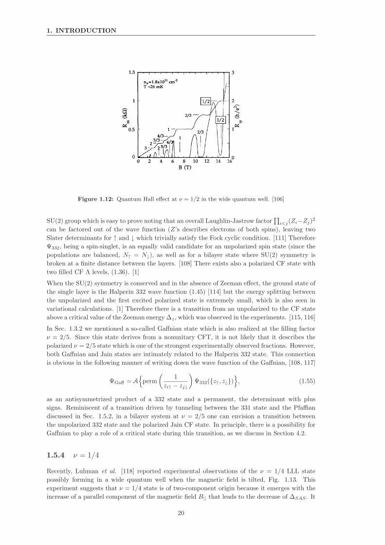
1. INTRODUCTION
Figure 1.12: Quantum Hall effect at ν = 1/2 in the wide quantum well. [106]
SU(2) group which is easy to prove noting that an overall Laughlin-Jastrow factor∏
i<j(Zi−Zj)2
can be factored out of the wave function (Z’s describes electrons of both spins), leaving two
Slater determinants for ↑ and ↓ which trivially satisfy the Fock cyclic condition. [111] Therefore
Ψ332, being a spin-singlet, is an equally valid candidate for an unpolarized spin state (since the
populations are balanced, N↑ = N↓), as well as for a bilayer state where SU(2) symmetry is
broken at a finite distance between the layers. [108] There exists also a polarized CF state with
two filled CF Λ levels, (1.36). [1]
When the SU(2) symmetry is conserved and in the absence of Zeeman effect, the ground state of
the single layer is the Halperin 332 wave function (1.45) [114] but the energy splitting between
the unpolarized and the first excited polarized state is extremely small, which is also seen in
variational calculations. [1] Therefore there is a transition from an unpolarized to the CF state
above a critical value of the Zeeman energy ∆z, which was observed in the experiments. [115, 116]
In Sec. 1.3.2 we mentioned a so-called Gaffnian state which is also realized at the filling factor
ν = 2/5. Since this state derives from a nonunitary CFT, it is not likely that it describes the
polarized ν = 2/5 state which is one of the strongest experimentally observed fractions. However,
both Gaffnian and Jain states are intimately related to the Halperin 332 state. This connection
is obvious in the following manner of writing down the wave function of the Gaffnian, [108, 117]
ΨGaff = A
perm
(
1
zi↑ − zj↓
)
Ψ332(z↑, z↓)
, (1.55)
as an antisymmetrized product of a 332 state and a permanent, the determinant with plus
signs. Reminiscent of a transition driven by tunneling between the 331 state and the Pfaffian
discussed in Sec. 1.5.2, in a bilayer system at ν = 2/5 one can envision a transition between
the unpolarized 332 state and the polarized Jain CF state. In principle, there is a possibility for
Gaffnian to play a role of a critical state during this transition, as we discuss in Section 4.2.
1.5.4 ν = 1/4
Recently, Luhman et al. [118] reported experimental observations of the ν = 1/4 LLL state
possibly forming in a wide quantum well when the magnetic field is tilted, Fig. 1.13. This
experiment suggests that ν = 1/4 state is of two-component origin because it emerges with the
increase of a parallel component of the magnetic field B|| that leads to the decrease of ∆SAS . It
20
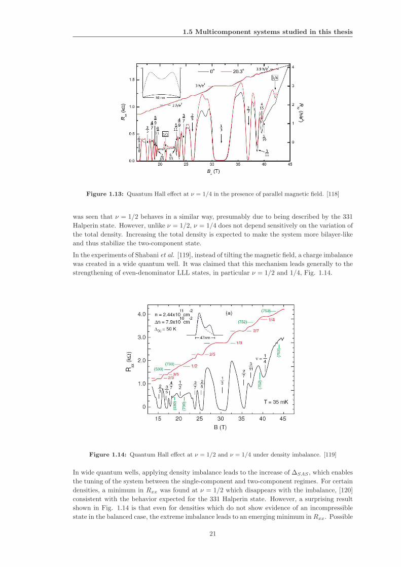
1.5 Multicomponent systems studied in this thesis
Figure 1.13: Quantum Hall effect at ν = 1/4 in the presence of parallel magnetic field. [118]
was seen that ν = 1/2 behaves in a similar way, presumably due to being described by the 331
Halperin state. However, unlike ν = 1/2, ν = 1/4 does not depend sensitively on the variation of
the total density. Increasing the total density is expected to make the system more bilayer-like
and thus stabilize the two-component state.
In the experiments of Shabani et al. [119], instead of tilting the magnetic field, a charge imbalance
was created in a wide quantum well. It was claimed that this mechanism leads generally to the
strengthening of even-denominator LLL states, in particular ν = 1/2 and 1/4, Fig. 1.14.
Figure 1.14: Quantum Hall effect at ν = 1/2 and ν = 1/4 under density imbalance. [119]
In wide quantum wells, applying density imbalance leads to the increase of ∆SAS , which enables
the tuning of the system between the single-component and two-component regimes. For certain
densities, a minimum in Rxx was found at ν = 1/2 which disappears with the imbalance, [120]
consistent with the behavior expected for the 331 Halperin state. However, a surprising result
shown in Fig. 1.14 is that even for densities which do not show evidence of an incompressible
state in the balanced case, the extreme imbalance leads to an emerging minimum in Rxx. Possible
21
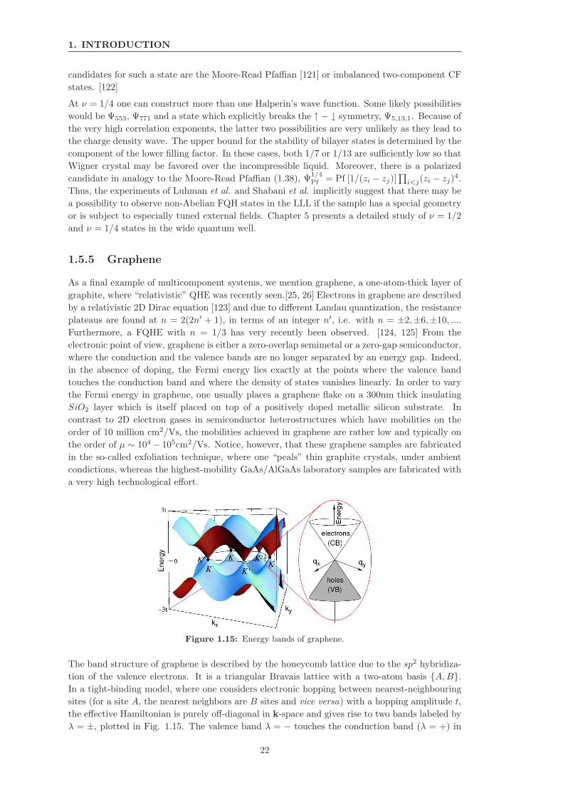
1. INTRODUCTION
candidates for such a state are the Moore-Read Pfaffian [121] or imbalanced two-component CF
states. [122]
At ν = 1/4 one can construct more than one Halperin’s wave function. Some likely possibilities
would be Ψ553, Ψ771 and a state which explicitly breaks the ↑ − ↓ symmetry, Ψ5,13,1. Because of
the very high correlation exponents, the latter two possibilities are very unlikely as they lead to
the charge density wave. The upper bound for the stability of bilayer states is determined by the
component of the lower filling factor. In these cases, both 1/7 or 1/13 are sufficiently low so that
Wigner crystal may be favored over the incompressible liquid. Moreover, there is a polarized
candidate in analogy to the Moore-Read Pfaffian (1.38), Ψ1/4Pf = Pf [1/(zi − zj)]
∏
i<j(zi − zj)4.
Thus, the experiments of Luhman et al. and Shabani et al. implicitly suggest that there may be
a possibility to observe non-Abelian FQH states in the LLL if the sample has a special geometry
or is subject to especially tuned external fields. Chapter 5 presents a detailed study of ν = 1/2
and ν = 1/4 states in the wide quantum well.
1.5.5 Graphene
As a final example of multicomponent systems, we mention graphene, a one-atom-thick layer of
graphite, where “relativistic” QHE was recently seen.[25, 26] Electrons in graphene are described
by a relativistic 2D Dirac equation [123] and due to different Landau quantization, the resistance
plateaus are found at n = 2(2n′ + 1), in terms of an integer n′, i.e. with n = ±2,±6,±10, ....
Furthermore, a FQHE with n = 1/3 has very recently been observed. [124, 125] From the
electronic point of view, graphene is either a zero-overlap semimetal or a zero-gap semiconductor,
where the conduction and the valence bands are no longer separated by an energy gap. Indeed,
in the absence of doping, the Fermi energy lies exactly at the points where the valence band
touches the conduction band and where the density of states vanishes linearly. In order to vary
the Fermi energy in graphene, one usually places a graphene flake on a 300nm thick insulating
SiO2 layer which is itself placed on top of a positively doped metallic silicon substrate. In
contrast to 2D electron gases in semiconductor heterostructures which have mobilities on the
order of 10 million cm2/Vs, the mobilities achieved in graphene are rather low and typically on
the order of µ ∼ 104 − 105cm2/Vs. Notice, however, that these graphene samples are fabricated
in the so-called exfoliation technique, where one “peals” thin graphite crystals, under ambient
condictions, whereas the highest-mobility GaAs/AlGaAs laboratory samples are fabricated with
a very high technological effort.
Figure 1.15: Energy bands of graphene.
The band structure of graphene is described by the honeycomb lattice due to the sp2 hybridiza-
tion of the valence electrons. It is a triangular Bravais lattice with a two-atom basis A,B.In a tight-binding model, where one considers electronic hopping between nearest-neighbouring
sites (for a site A, the nearest neighbors are B sites and vice versa) with a hopping amplitude t,
the effective Hamiltonian is purely off-diagonal in k-space and gives rise to two bands labeled by
λ = ±, plotted in Fig. 1.15. The valence band λ = − touches the conduction band (λ = +) in
22
1.5 Multicomponent systems studied in this thesis
the two inequivalent corners K and K ′ of the first Brillouin zone. The Fermi energy lies exactly
in the contact points K and K ′ of the two bands unless the graphene sheet is doped. The inset
in Fig. 1.15 shows the band dispersion in the vicinity of the contact points K and K ′, the
linearity of which is sufficient to describe the low-energy electronic properties in graphene. The
conical form of the two bands is reminiscent of that of relativistic particles, which is also obvious
from the Dirac form of the Hamiltonian when it is expressed around K point, H = vσ · p. In
the continuum description of electrons in graphene we have two electron types, for the K and
K ′ point, which is the valley degeneracy. Together with the usual spin degeneracy, graphene is
implicitly a four-component system which is therefore characterized by a wave function which
is a SU(4)-spinor. The energy scale for lifting the valley/spin degeneracy are similar and much
smaller than the one set by the Coulomb interactions. SU(K) internal symmetry (approximately
realized in some range of the system parameters) can nonetheless be described with a simple
instance of the wave function (1.47) for K = 4 that is expected to describe quantized states in
four-component systems. Note that the exponents nij and njj ≡ mj define a symmetric 4 × 4
matrix M = (nij), which determines the component densities ρj – or else the component filling
factors νj = ρj/nB ,
ν1ν2ν3ν4
= M−1
1
1
1
1
. (1.56)
Eq. (1.56) is only well-defined if the matrix M is invertible. If M is not invertible, some of the
component filling factors, e.g. ν1 and ν2, remain unfixed, but not necessarily the sum of the
two (ν1 + ν2). This is a particular feature of possible underlying ferromagnetic properties of the
wave function, [126] as we discussed in Sec. 1.4. The component filling factors in this context
are those that arise naturally in FQHE studies, i.e. they are defined with respect to the bottom
of the partially filled LL, in contrast to the graphene filling factor, νG, defined with respect to
the center of n = 0 level. In order to make the connection between the two filling factors, one
needs to choose
ν = ν1 + ν2 + ν3 + ν4 = νG + 2. (1.57)
In Chapter 6 we consider some particular subclasses of the trial wave functions (1.47), which are
natural candidates for a FQHE in graphene.
23
1. INTRODUCTION
24
Chapter 2
Numerical studies of the FQHE
In this Chapter we set up the numerical (exact) diagonalization of the FQH problem in finite
geometries. Throughout this thesis, by exact diagonalization (ED) we refer to the procedure
where the Hamiltonian of the system, subject to particular boundary conditions, is represented
in a convenient (finite) basis and its energy spectrum numerically evaluated using the computer.
This method offers the possibility to study the quantum system in an unbiased manner and it was
used since the early days of the FQHE, for example in working out the physical properties of the
Laughlin wave function. [41] By now it has assumed the status of a standard tool in FQH studies
where perturbative approaches are not guaranteed to work and physical properties expected in
the thermodynamic limit can be identified already in very small systems. Although the energy
spectrum itself offers substantial information about the physical system, it is furthermore possible
to make direct comparison between the numerically-obtained eigenvector and the given trial
wave function believed to describe the system’s state. This amounts to evaluating a simple
scalar product between the two vectors and we refer to it as the overlap calculation. Knowledge
of the eigenvectors also allows one to calculate various operator mean values, propagators etc.
The virtue of exact diagonalization is its versatility because it can be applied to any system.
However, in practice the computational effort exponentially increases with the size of the system
and therefore ED is usually restricted to small systems. Despite this, ED remains a powerful
tool of choice for the theoretical studies of the FQHE.
Popular choices of the geometry in the FQH literature have been the disk [42], the sphere [127]
and the rectangle with periodic boundary conditions (torus) [128]. In this thesis we focus on the
latter two geometries which do not have open boundaries and therefore are particularly useful
in examining the bulk properties of incompressible FQH liquids. This Chapter will largely
present an overview of the pioneering papers by Haldane [42, 127, 129] and their extensions.
[1, 18, 21, 130]
2.1 Exact diagonalization: Sphere
The original insight of Haldane [127] was that the two-dimensional sheet containing electrons
can be wrapped around the surface of a sphere, while the perpendicular (radial) magnetic field
is generated by a fictitious Dirac magnetic monopole at the sphere’s center. The single particle
problem had previously been solved by Wu and Yang. [131, 132] We will quote the main results
without derivation. A recent pedagogical summary containing some of the derivations is given
in [1].
The magnetic flux through the surface of the sphere (measured in units of Φ0), is quantized to
be an integer and denoted by Nφ = 2Q. The position of an electron is given by the spherical
coordinates R =√QlB , θ, φ. Because of the rotational symmetry enforced by the choice of
25
2. NUMERICAL STUDIES OF THE FQHE
the geometry, the orbital angular momentum and its z-component are good quantum numbers,
denoted by l and m, respectively. Due to the presence of the monopole, their allowed values are
l = |Q|, |Q|+ 1, . . . and m = −l,−l+ 1, . . . , l. Different angular momentum shells correspond to
Landau levels in the spherical geometry. The degeneracy of each Landau level is equal to the
total number of m values, i.e. 2l + 1, it is obviously finite and increasing by two units for each
successive Landau level. The single particle eigenstates are the monopole harmonics, denoted
by YQlm, which are a generalization of the familiar spherical harmonics for Q = 0. In the lowest
Landau level, they reduce to
YQQm =
√
2Q+ 1
4π
(
2Q
2Q−m
)
(−1)Q−mvQ−muQ+m, (2.1)
where u, v are the spinor variables [127]
u = cos θ/2eiφ/2, v = sin θ/2e−iφ/2. (2.2)
The spinor variables are not independent because |u|2+ |v|2 = 1 and we can transform to a single
z complex coordinate by stereographic mapping z = 2Rv/u, R being the radius of the sphere.
The basis states are given by zm/(1 + |z|2/4R2)1+Nφ/2, where the Lz momentum quantum
number is Lz = Nφ/2 −m. Note that if Nφ, R → ∞ (with Nφ/R2 fixed), the sphere becomes
effectively flat and the single particle states reduce to those on the disk, zme−|z|2/4.
For N electrons, the filling factor corresponding to the thermodynamic limit (1.8) is given by
ν = limN→∞
N
2|Q| , (2.3)
but in case of the finite system the relation (2.3) requires a slight modification:
Nφ =1
νN − δ, (2.4)
which defines the so-called shift, δ. The shift is the topological number that characterizes each
FQH state on the spherical surface. It is of order unity (e.g. the Laughlin state at ν = 1/3
has δ = 3) and it is required to specify the system in addition to the filling factor ν. In the
thermodynamic limit of an infinite plane, the shift plays no role, but for a finite sphere it is a
crucial aspect of the ED technique [42] as it can lead to an “aliasing” problem: at a fixed choice
of (Nφ, N), more than one quantum Hall state (having different ν, δ and, therefore, different
physical properties) may be realized.
We are now in a position to set up the Hilbert space which contains the Slater determinants
|m1,m2, . . . ,mN 〉 = c†m1. . . c†mN
|0〉 built from the single-particle states labelled by mi. It is
often advantageous to exploit symmetries in order to reduce the dimension of the Hamiltonian
matrix because we only consider transtionally/rotationally invariant Hamiltonians. An obvious
symmetry which is used in the construction of Hilbert space is the conservation of Lz =∑
imi
component. In principle it is possible to demand full rotational symmetry and diagonalize the
Hamiltonian in the invariant subspaces of the L2 operator, but the numerical implementation of
this symmetry is difficult. One can also use the symmetry under the discrete parity transforma-
tion Lz → −Lz in diagonalizing within Lz = 0 sector of the Hilbert space.
The general interacting Hamiltonian in the basis of states |m1,m2, . . . ,mN 〉 , expressed in second-
quantized form, is given by
H =1
2
Q∑
m1,m2,m3,m4=−Q
〈m1,m2|V |m3m4〉c†m1c†m2
cm4cm3. (2.5)
26
2.1 Exact diagonalization: Sphere
The interaction V usually is such that it depends solely on the relative coordinate and not
the center of mass. This is the case for Coulomb (1.9) and any other physical interaction.
Furthermore, if the interaction involves only two particles at a time, it is convenient to express
the matrix element 〈m1,m2|V |m3,m4〉 in the following form
〈m1,m2|V |m3,m4〉 =
2Q∑
L=0
L∑
m=−L
〈Qm1, Qm2|L,M〉V2Q−L〈L,M |Qm3, Qm4〉 (2.6)
where the numbers V2Q−L are called the Haldane pseudopotentials and can be directly evaluated
(a useful formula for the Coulomb interaction in the LLL is given in [130]). Evaluated on the
sphere, V2Q−L represents the energy of two particles in a state with relative angular momentum
L in the plane. Apart from geometrical Clebsch-Gordan coefficients 〈L,M |Qmi, Qmj〉, the set
of VL|L = 0, . . . , 2Q uniquely specifies the interacting Hamiltonian in any one Landau level.
If the particles are fermions, the only physically relevant pseudopotentials are those with odd
2Q − L because of the exchange antisymmetry. Using the algebra of the harmonic oscillator
raising operators, it can be shown that the Fourier transform of the effective interaction Veff
of the nth LL projected to the LLL is simply related to the Fourier transform of the LLL
interaction V : Veff(k) =[
Ln(k2
2 )]2
V (k). Therefore, as long as we remain in a single Landau
level, the problem is uniquely specified by a simple sequence of numbers VL. Another important
insight also due to Haldane [42] was that specifying a few non-zero VL’s defines special short-
range Hamiltonians that uniquely produce certain FQH trial states as their zero-energy modes.
The simplest example is the Laughlin state at ν = 1/3 which is the unique, highest density zero
mode of the following pseudopotential Hamiltonian:
V1 > 0, V3 = V5 = . . . = 0 (2.7)
This is the hard-core interaction that is represented by (1.22) in the real space. We can numer-
ically obtain the ground state of the interaction (2.7), inserting (2.7) into the Hamiltonian (2.5)
and choosing the proper shift Nφ = 3N − 3. We will recover a unique zero-energy state with a
gap controlled by the value of V1 and a magneto-roton branch in the excitation spectrum, [45]
the known facts from the physics of the Laughlin state (Sec. 2.2.1).
2.1.1 Example: Effect of finite thickness on the Laughlin ν = 1/3 state
To illustrate the principle of numerical investigation, let us try to tackle the following simple
problem: what is the effect of finite layer width on the ν = 1/3 state. We can model the
finite-width FQH system using the effective Zhang-Das Sarma interaction, (1.17). We evaluate
the Haldane pseudopotentials for the ZDS interaction, numerically diagonalize the Hamiltonian
(2.5) for several values of the width parameter d and obtain the exact eigenvectors |Ψexact〉. On
the other hand, the ground state of the interaction (2.7) is just the Laughlin state |ΨL〉. By
evaluating the scalar product between the two vectors, 〈ΨL|Ψexact〉, we can monitor how well the
Laughlin wave function describes the exact ground state. We know that for d = 0 the overlap is
very large (nearly 1), which means that the Laughlin wave function is an excellent representative
of the ground state. More details on the numerical calculations are given in the Appendix. The
results for several values of d are given in Fig. 2.1. We see that the overlap decreases with
the thickness of the sample, which is consistent with the experiments that see the weakening of
the Laughlin state in the samples of very wide width. In the inset to Fig. 2.1 we repeated the
calculation for the first excited LL, using the effective interaction Veff as we explained above.
Here we may note that the Laughlin state is a much worse description of the exact state for
small values of d. Indeed, for N = 5 particles we even obtain zero overlap. Small overlap usually
means that we have a wrong candidate wave function. Zero overlap, on the other hand, means
that we are testing wave functions of different symmetry, e.g. an incompressible L = 0 state
27
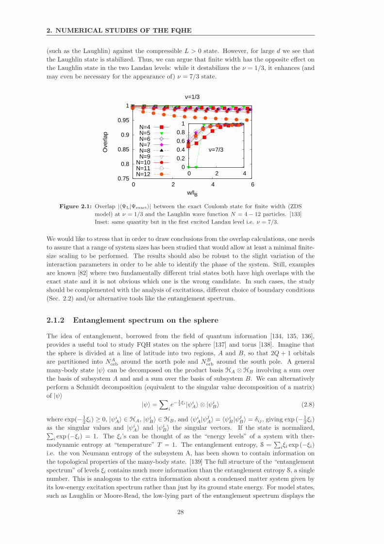
2. NUMERICAL STUDIES OF THE FQHE
(such as the Laughlin) against the compressible L > 0 state. However, for large d we see that
the Laughlin state is stabilized. Thus, we can argue that finite width has the opposite effect on
the Laughlin state in the two Landau levels: while it destabilizes the ν = 1/3, it enhances (and
may even be necessary for the appearance of) ν = 7/3 state.
0.75
0.8
0.85
0.9
0.95
1
0 2 4 6
Ove
rlap
w/lB
ν=1/3
N=4N=5N=6N=7N=8N=9
N=10N=11N=12
0
0.2
0.4
0.6
0.8
1
0 2 4
ν=7/3
Figure 2.1: Overlap |〈ΨL|Ψexact〉| between the exact Coulomb state for finite width (ZDS
model) at ν = 1/3 and the Laughlin wave function N = 4 − 12 particles. [133]
Inset: same quantity but in the first excited Landau level i.e. ν = 7/3.
We would like to stress that in order to draw conclusions from the overlap calculations, one needs
to assure that a range of system sizes has been studied that would allow at least a minimal finite-
size scaling to be performed. The results should also be robust to the slight variation of the
interaction parameters in order to be able to identify the phase of the system. Still, examples
are known [82] where two fundamentally different trial states both have high overlaps with the
exact state and it is not obvious which one is the wrong candidate. In such cases, the study
should be complemented with the analysis of excitations, different choice of boundary conditions
(Sec. 2.2) and/or alternative tools like the entanglement spectrum.
2.1.2 Entanglement spectrum on the sphere
The idea of entanglement, borrowed from the field of quantum information [134, 135, 136],
provides a useful tool to study FQH states on the sphere [137] and torus [138]. Imagine that
the sphere is divided at a line of latitude into two regions, A and B, so that 2Q + 1 orbitals
are partitioned into NAorb around the north pole and NB
orb around the south pole. A general
many-body state |ψ〉 can be decomposed on the product basis HA ⊗HB involving a sum over
the basis of subsystem A and and a sum over the basis of subsystem B. We can alternatively
perform a Schmidt decomposition (equivalent to the singular value decomposition of a matrix)
of |ψ〉|ψ〉 =
∑
ie−
12ξi |ψi
A〉 ⊗ |ψiB〉 (2.8)
where exp(− 12ξi) ≥ 0, |ψi
A〉 ∈ HA, |ψiB〉 ∈ HB , and 〈ψi
A|ψjA〉 = 〈ψi
B |ψjB〉 = δij , giving exp (− 1
2ξi)
as the singular values and |ψiA〉 and |ψi
B〉 the singular vectors. If the state is normalized,∑
i exp (−ξi) = 1. The ξi’s can be thought of as the “energy levels” of a system with ther-
modynamic entropy at “temperature” T = 1. The entanglement entropy, S =∑
iξi exp (−ξi)i.e. the von Neumann entropy of the subsystem A, has been shown to contain information on
the topological properties of the many-body state. [139] The full structure of the “entanglement
spectrum” of levels ξi contains much more information than the entanglement entropy S, a single
number. This is analogous to the extra information about a condensed matter system given by
its low-energy excitation spectrum rather than just by its ground state energy. For model states,
such as Laughlin or Moore-Read, the low-lying part of the entanglement spectrum displays the
28
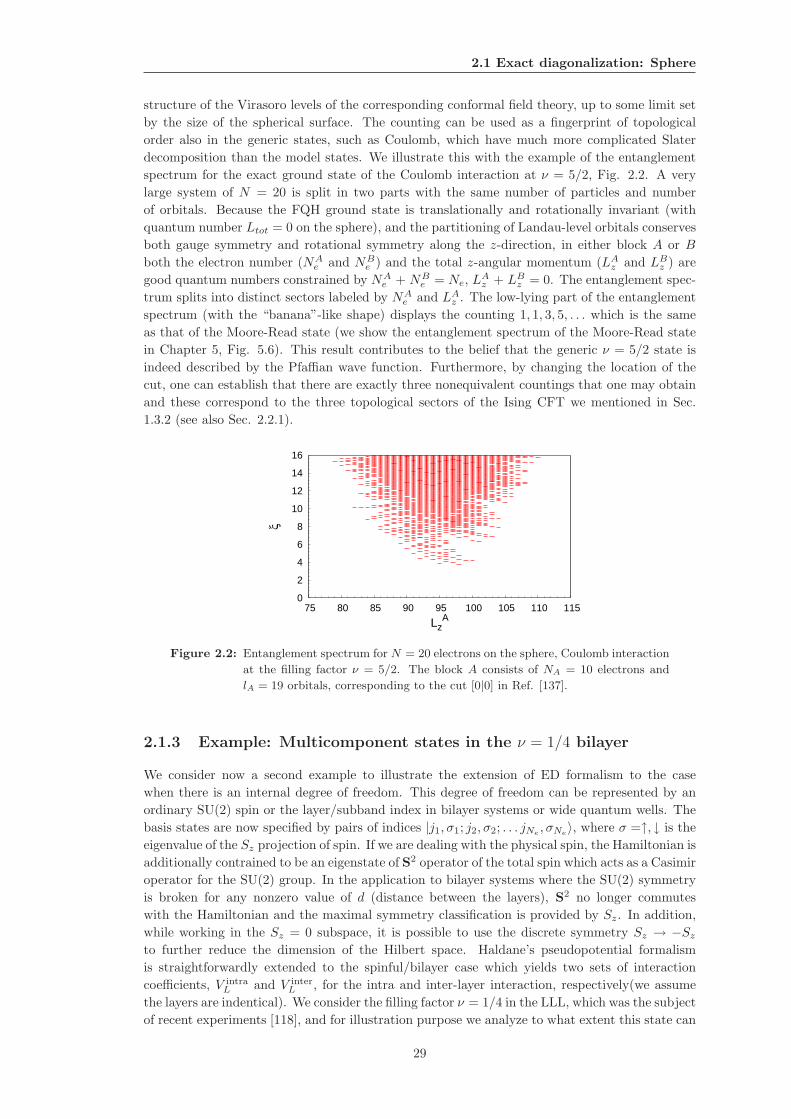
2.1 Exact diagonalization: Sphere
structure of the Virasoro levels of the corresponding conformal field theory, up to some limit set
by the size of the spherical surface. The counting can be used as a fingerprint of topological
order also in the generic states, such as Coulomb, which have much more complicated Slater
decomposition than the model states. We illustrate this with the example of the entanglement
spectrum for the exact ground state of the Coulomb interaction at ν = 5/2, Fig. 2.2. A very
large system of N = 20 is split in two parts with the same number of particles and number
of orbitals. Because the FQH ground state is translationally and rotationally invariant (with
quantum number Ltot = 0 on the sphere), and the partitioning of Landau-level orbitals conserves
both gauge symmetry and rotational symmetry along the z-direction, in either block A or B
both the electron number (NAe and NB
e ) and the total z-angular momentum (LAz and LB
z ) are
good quantum numbers constrained by NAe + NB
e = Ne, LAz + LB
z = 0. The entanglement spec-
trum splits into distinct sectors labeled by NAe and LA
z . The low-lying part of the entanglement
spectrum (with the “banana”-like shape) displays the counting 1, 1, 3, 5, . . . which is the same
as that of the Moore-Read state (we show the entanglement spectrum of the Moore-Read state
in Chapter 5, Fig. 5.6). This result contributes to the belief that the generic ν = 5/2 state is
indeed described by the Pfaffian wave function. Furthermore, by changing the location of the
cut, one can establish that there are exactly three nonequivalent countings that one may obtain
and these correspond to the three topological sectors of the Ising CFT we mentioned in Sec.
1.3.2 (see also Sec. 2.2.1).
0
2
4
6
8
10
12
14
16
75 80 85 90 95 100 105 110 115
ξ
LzA
Figure 2.2: Entanglement spectrum for N = 20 electrons on the sphere, Coulomb interaction
at the filling factor ν = 5/2. The block A consists of NA = 10 electrons and
lA = 19 orbitals, corresponding to the cut [0|0] in Ref. [137].
2.1.3 Example: Multicomponent states in the ν = 1/4 bilayer
We consider now a second example to illustrate the extension of ED formalism to the case
when there is an internal degree of freedom. This degree of freedom can be represented by an
ordinary SU(2) spin or the layer/subband index in bilayer systems or wide quantum wells. The
basis states are now specified by pairs of indices |j1, σ1; j2, σ2; . . . jNe, σNe
〉, where σ =↑, ↓ is the
eigenvalue of the Sz projection of spin. If we are dealing with the physical spin, the Hamiltonian is
additionally contrained to be an eigenstate of S2 operator of the total spin which acts as a Casimir
operator for the SU(2) group. In the application to bilayer systems where the SU(2) symmetry
is broken for any nonzero value of d (distance between the layers), S2 no longer commutes
with the Hamiltonian and the maximal symmetry classification is provided by Sz. In addition,
while working in the Sz = 0 subspace, it is possible to use the discrete symmetry Sz → −Sz
to further reduce the dimension of the Hilbert space. Haldane’s pseudopotential formalism
is straightforwardly extended to the spinful/bilayer case which yields two sets of interaction
coefficients, V intraL and V inter
L , for the intra and inter-layer interaction, respectively(we assume
the layers are indentical). We consider the filling factor ν = 1/4 in the LLL, which was the subject
of recent experiments [118], and for illustration purpose we analyze to what extent this state can
29
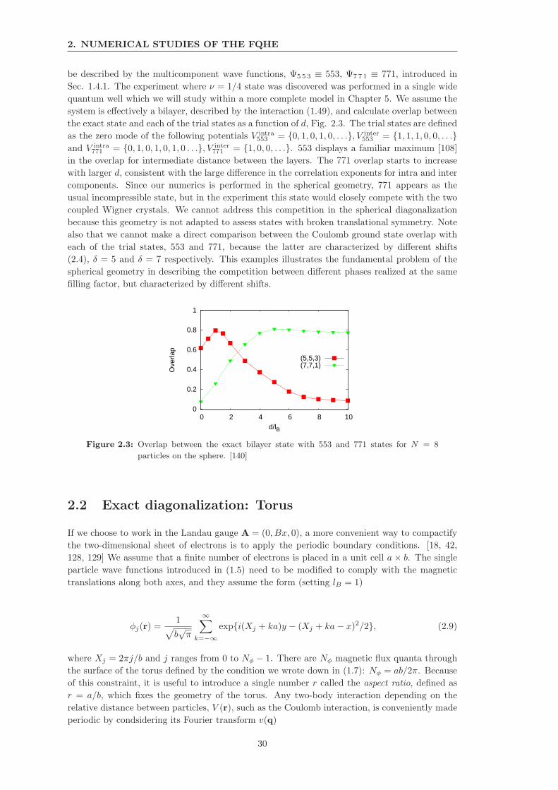
2. NUMERICAL STUDIES OF THE FQHE
be described by the multicomponent wave functions, Ψ5 5 3 ≡ 553, Ψ7 7 1 ≡ 771, introduced in
Sec. 1.4.1. The experiment where ν = 1/4 state was discovered was performed in a single wide
quantum well which we will study within a more complete model in Chapter 5. We assume the
system is effectively a bilayer, described by the interaction (1.49), and calculate overlap between
the exact state and each of the trial states as a function of d, Fig. 2.3. The trial states are defined
as the zero mode of the following potentials V intra553 = 0, 1, 0, 1, 0, . . ., V inter
553 = 1, 1, 1, 0, 0, . . .and V intra
771 = 0, 1, 0, 1, 0, 1, 0 . . ., V inter771 = 1, 0, 0, . . .. 553 displays a familiar maximum [108]
in the overlap for intermediate distance between the layers. The 771 overlap starts to increase
with larger d, consistent with the large difference in the correlation exponents for intra and inter
components. Since our numerics is performed in the spherical geometry, 771 appears as the
usual incompressible state, but in the experiment this state would closely compete with the two
coupled Wigner crystals. We cannot address this competition in the spherical diagonalization
because this geometry is not adapted to assess states with broken translational symmetry. Note
also that we cannot make a direct comparison between the Coulomb ground state overlap with
each of the trial states, 553 and 771, because the latter are characterized by different shifts
(2.4), δ = 5 and δ = 7 respectively. This examples illustrates the fundamental problem of the
spherical geometry in describing the competition between different phases realized at the same
filling factor, but characterized by different shifts.
0
0.2
0.4
0.6
0.8
1
0 2 4 6 8 10
Ove
rlap
d/lB
(5,5,3)(7,7,1)
Figure 2.3: Overlap between the exact bilayer state with 553 and 771 states for N = 8
particles on the sphere. [140]
2.2 Exact diagonalization: Torus
If we choose to work in the Landau gauge A = (0, Bx, 0), a more convenient way to compactify
the two-dimensional sheet of electrons is to apply the periodic boundary conditions. [18, 42,
128, 129] We assume that a finite number of electrons is placed in a unit cell a × b. The single
particle wave functions introduced in (1.5) need to be modified to comply with the magnetic
translations along both axes, and they assume the form (setting lB = 1)
φj(r) =1
√
b√π
∞∑
k=−∞expi(Xj + ka)y − (Xj + ka− x)2/2, (2.9)
where Xj = 2πj/b and j ranges from 0 to Nφ − 1. There are Nφ magnetic flux quanta through
the surface of the torus defined by the condition we wrote down in (1.7): Nφ = ab/2π. Because
of this constraint, it is useful to introduce a single number r called the aspect ratio, defined as
r = a/b, which fixes the geometry of the torus. Any two-body interaction depending on the
relative distance between particles, V (r), such as the Coulomb interaction, is conveniently made
periodic by condsidering its Fourier transform v(q)
30
2.2 Exact diagonalization: Torus
V (r) =1
ab
′∑
q
v(q)eiqr, (2.10)
where q takes values in the first Brillouin zone q = (2πs/a, 2πt/b) (s, t are integers) and where
v(q) = 2πe2/ǫ|q| is the Fourier-transformed Coulomb interaction. The prime on the sum in
(2.10) indicates that the q = 0 component has been cancelled by the uniform positive background
charge. Using (2.10) and (2.9), the matrix elements can be calculated [18] and the interaction
part of the Hamiltonian is again defined by (2.5). Apart from the two-body interaction terms,
the Hamiltonian contains the one-body terms which result from the interaction of the electrons
with their mirror images (a consequence of the periodic boundary condition). These one-body
terms depend only on the geometry of the torus and can be dropped from the Hamiltonian as
long as the aspect ratio is held fixed.
As in the case of the spherical geometry, it is useful to use symmetries in order to reduce the
dimension of the Hamiltonian matrix to be diagonalized, but instead of rotational symmetry one
must consider on the torus the magnetic translations along the x and y axes. The full treatment
of the magnetic translation symmetry in this context was first given by Haldane. [129] The
magnetic translation operator acting on a particle j is defined as
Tj(L) = exp (− i~L ·Kj), (2.11)
where the crystal momentum is Kj = −pj − eByjex. Consistency requires that encircling the
torus around the perimeter of the unit cell produces an identity operation, which yields the
condition ez · (a×b) = 2πNφ. Let us consider now a many-body system of Ne electrons and Nφ
flux quanta, so the filling factor ν = Ne/Nφ can be expressed in the reduced form ν = p/q, where
p, q are coprime numbers. Then we also have Ne = pN ′, Nφ = qN ′, where N ′ is the greatest
common divisor of Ne and Nφ. The center of mass translation operator simply translates each
of the particles independently, T (L) =∏
j Tj(L). If the single particle wave functions are to be
unaffected by such a transformation, we find that the most general translation is for the vector
L =1
NφLmn,
where Lmn = (ma, nb). Center of mass translations give rise to a degeneracy of q for each state
at the filling factor ν = p/q. [18, 129] Physical information is contained in the eigenvalues of the
relative translations
Tj(L) =∏
i
Tj(L/Ne)Ti(L/Ne). (2.12)
It can be shown that the spectrum of the operators of relative translations Tj consists of N ′2
points in the inverse lattice, labeled by integers s, t = 0, . . . , N ′ − 1. These numbers are the
fundamental quantum numbers that classify the physical eigenstates of the Hamiltonian. They
are related to the physical momentum via
k =
√
2π
Nφr[s− s0, r(t− t0)] (2.13)
where (s0, t0) corresponds to the zero momentum fixed by
ei2πs0/N ′
= ei2πt0/N ′
= (−1)pq(Ne−1). (2.14)
The incompressible states such as Laughlin’s in this notation are characterized by k = 0 ground
state and a gap to all excitations. The construction of the symmetry-adapted basis proceeds
31
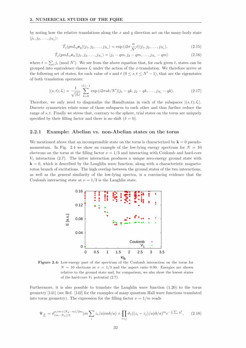
2. NUMERICAL STUDIES OF THE FQHE
by noting how the relative translations along the x and y direction act on the many-body state
|j1, j2, . . . , jNe〉:
Tj(pnLyey)|j1, j2, . . . , jNe〉 = exp (i2π
n
N ′ t)|j1, j2, . . . , jNe〉, (2.15)
Tj(pmLxex)|j1, j2, . . . , jNe〉 = |j1 − qm, j2 − qm, . . . , jNe
− qm〉 (2.16)
where t =∑
i ji (mod N ′). We see from the above equation that, for each given t, states can be
grouped into equivalence classes L under the action of the x-translation. We therefore arrive at
the following set of states, for each value of s and t (0 ≤ s, t ≤ N ′ − 1), that are the eigenstates
of both translation operators:
|(s, t);L〉 =1
√
|L|
|L|−1∑
k=0
exp (i2πsk/N ′)|j1 − qk, j2 − qk, . . . , jNe− qk〉. (2.17)
Therefore, we only need to diagonalize the Hamiltonian in each of the subspaces |(s, t);L〉.Discrete symmetries relate some of those subspaces to each other and thus further reduce the
range of s, t. Finally we stress that, contrary to the sphere, trial states on the torus are uniquely
specified by their filling factor and there is no shift (δ = 0).
2.2.1 Example: Abelian vs. non-Abelian states on the torus
We mentioned above that an incompressible state on the torus is characterized by k = 0 pseudo-
momentum. In Fig. 2.4 we show an example of the low-lying energy spectrum for N = 10
electrons on the torus at the filling factor ν = 1/3 and interacting with Coulomb and hard-core
V1 interaction (2.7). The latter interaction produces a unique zero-energy ground state with
k = 0, which is described by the Laughlin wave function, along with a characteristic magneto-
roton branch of excitations. The high overlap between the ground states of the two interactions,
as well as the general similarity of the low-lying spectra, is a convincing evidence that the
Coulomb interacting state at ν = 1/3 is the Laughlin state.
0
0.04
0.08
0.12
0.16
0 0.5 1 1.5 2 2.5 3 3.5
E [a
.u.]
klB
CoulombV1
Figure 2.4: Low-energy part of the spectrum of the Coulomb interaction on the torus for
N = 10 electrons at ν = 1/3 and the aspect ratio 0.99. Energies are shown
relative to the ground state and, for comparison, we also show the lowest states
of the hard-core V1 potential (2.7).
Furthermore, it is also possible to translate the Laughlin wave function (1.20) to the torus
geometry [141] (see Ref. [142] for the examples of many quantum Hall wave functions translated
into torus geometry). The expression for the filling factor ν = 1/m reads
Ψ 1m
= ϑα/m+(Nφ−m)/2m
(m−Nφ)/2 (m∑
i
zi/a|imb/a)×∏
i<j
ϑ1((zi − zj)/a|ib/a)me−12
P
i y2i , (2.18)
32
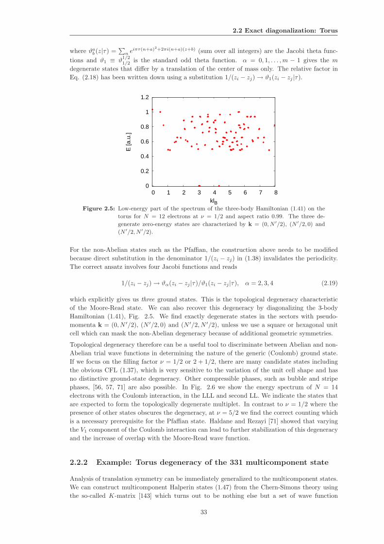
2.2 Exact diagonalization: Torus
where ϑab (z|τ) =
∑
n eiπτ(n+a)2+2πi(n+a)(z+b) (sum over all integers) are the Jacobi theta func-
tions and ϑ1 ≡ ϑ1/21/2 is the standard odd theta function. α = 0, 1, . . . ,m − 1 gives the m
degenerate states that differ by a translation of the center of mass only. The relative factor in
Eq. (2.18) has been written down using a substitution 1/(zi − zj)→ ϑ1(zi − zj |τ).
0
0.2
0.4
0.6
0.8
1
1.2
0 1 2 3 4 5 6 7 8
E [a
.u.]
klBFigure 2.5: Low-energy part of the spectrum of the three-body Hamiltonian (1.41) on the
torus for N = 12 electrons at ν = 1/2 and aspect ratio 0.99. The three de-
generate zero-energy states are characterized by k = (0, N ′/2), (N ′/2, 0) and
(N ′/2, N ′/2).
For the non-Abelian states such as the Pfaffian, the construction above needs to be modified
because direct substitution in the denominator 1/(zi − zj) in (1.38) invalidates the periodicity.
The correct ansatz involves four Jacobi functions and reads
1/(zi − zj)→ ϑα(zi − zj |τ)/ϑ1(zi − zj |τ), α = 2, 3, 4 (2.19)
which explicitly gives us three ground states. This is the topological degeneracy characteristic
of the Moore-Read state. We can also recover this degeneracy by diagonalizing the 3-body
Hamiltonian (1.41), Fig. 2.5. We find exactly degenerate states in the sectors with pseudo-
momenta k = (0, N ′/2), (N ′/2, 0) and (N ′/2, N ′/2), unless we use a square or hexagonal unit
cell which can mask the non-Abelian degeneracy because of additional geometric symmetries.
Topological degeneracy therefore can be a useful tool to discriminate between Abelian and non-
Abelian trial wave functions in determining the nature of the generic (Coulomb) ground state.
If we focus on the filling factor ν = 1/2 or 2 + 1/2, there are many candidate states including
the obvious CFL (1.37), which is very sensitive to the variation of the unit cell shape and has
no distinctive ground-state degeneracy. Other compressible phases, such as bubble and stripe
phases, [56, 57, 71] are also possible. In Fig. 2.6 we show the energy spectrum of N = 14
electrons with the Coulomb interaction, in the LLL and second LL. We indicate the states that
are expected to form the topologically degenerate multiplet. In contrast to ν = 1/2 where the
presence of other states obscures the degeneracy, at ν = 5/2 we find the correct counting which
is a necessary prerequisite for the Pfaffian state. Haldane and Rezayi [71] showed that varying
the V1 component of the Coulomb interaction can lead to further stabilization of this degeneracy
and the increase of overlap with the Moore-Read wave function.
2.2.2 Example: Torus degeneracy of the 331 multicomponent state
Analysis of translation symmetry can be immediately generalized to the multicomponent states.
We can construct multicomponent Halperin states (1.47) from the Chern-Simons theory using
the so-called K-matrix [143] which turns out to be nothing else but a set of wave function
33
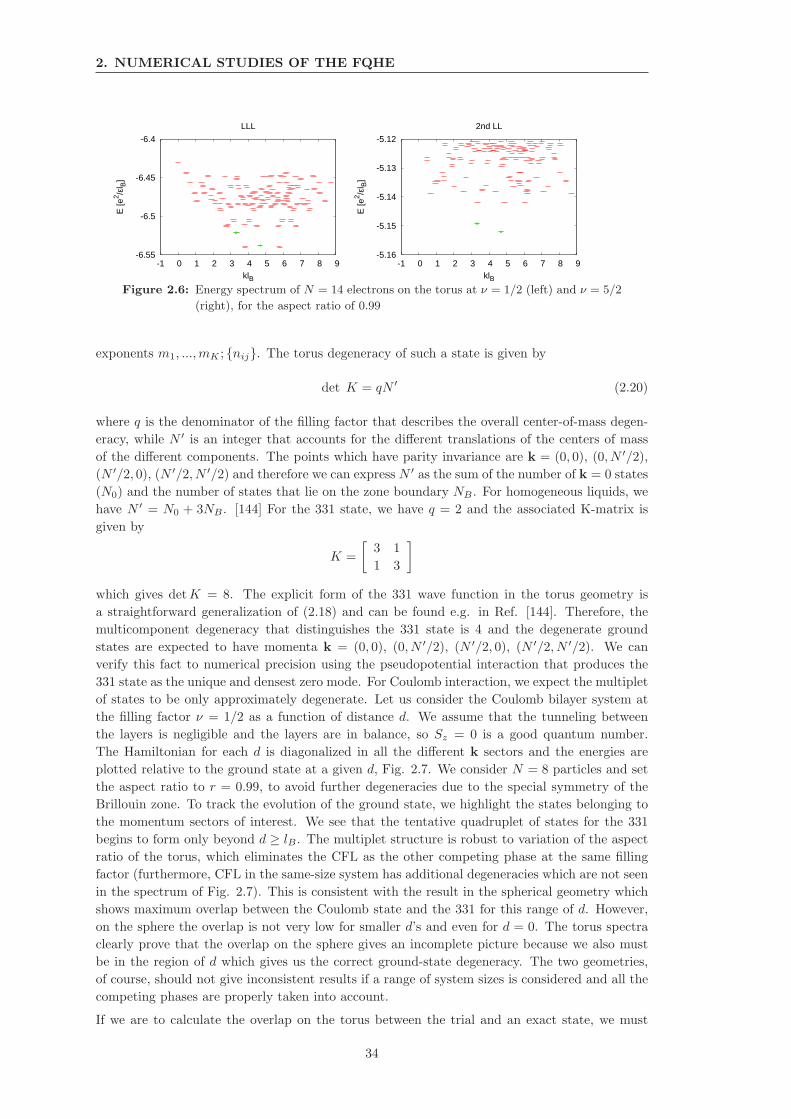
2. NUMERICAL STUDIES OF THE FQHE
-6.55
-6.5
-6.45
-6.4
-1 0 1 2 3 4 5 6 7 8 9
E [e
2 /εl B
]
klB
LLL
-5.16
-5.15
-5.14
-5.13
-5.12
-1 0 1 2 3 4 5 6 7 8 9
E [e
2 /εl B
]
klB
2nd LL
Figure 2.6: Energy spectrum of N = 14 electrons on the torus at ν = 1/2 (left) and ν = 5/2
(right), for the aspect ratio of 0.99
exponents m1, ...,mK ; nij. The torus degeneracy of such a state is given by
det K = qN ′ (2.20)
where q is the denominator of the filling factor that describes the overall center-of-mass degen-
eracy, while N ′ is an integer that accounts for the different translations of the centers of mass
of the different components. The points which have parity invariance are k = (0, 0), (0, N ′/2),
(N ′/2, 0), (N ′/2, N ′/2) and therefore we can express N ′ as the sum of the number of k = 0 states
(N0) and the number of states that lie on the zone boundary NB . For homogeneous liquids, we
have N ′ = N0 + 3NB . [144] For the 331 state, we have q = 2 and the associated K-matrix is
given by
K =
[
3 1
1 3
]
which gives detK = 8. The explicit form of the 331 wave function in the torus geometry is
a straightforward generalization of (2.18) and can be found e.g. in Ref. [144]. Therefore, the
multicomponent degeneracy that distinguishes the 331 state is 4 and the degenerate ground
states are expected to have momenta k = (0, 0), (0, N ′/2), (N ′/2, 0), (N ′/2, N ′/2). We can
verify this fact to numerical precision using the pseudopotential interaction that produces the
331 state as the unique and densest zero mode. For Coulomb interaction, we expect the multiplet
of states to be only approximately degenerate. Let us consider the Coulomb bilayer system at
the filling factor ν = 1/2 as a function of distance d. We assume that the tunneling between
the layers is negligible and the layers are in balance, so Sz = 0 is a good quantum number.
The Hamiltonian for each d is diagonalized in all the different k sectors and the energies are
plotted relative to the ground state at a given d, Fig. 2.7. We consider N = 8 particles and set
the aspect ratio to r = 0.99, to avoid further degeneracies due to the special symmetry of the
Brillouin zone. To track the evolution of the ground state, we highlight the states belonging to
the momentum sectors of interest. We see that the tentative quadruplet of states for the 331
begins to form only beyond d ≥ lB . The multiplet structure is robust to variation of the aspect
ratio of the torus, which eliminates the CFL as the other competing phase at the same filling
factor (furthermore, CFL in the same-size system has additional degeneracies which are not seen
in the spectrum of Fig. 2.7). This is consistent with the result in the spherical geometry which
shows maximum overlap between the Coulomb state and the 331 for this range of d. However,
on the sphere the overlap is not very low for smaller d’s and even for d = 0. The torus spectra
clearly prove that the overlap on the sphere gives an incomplete picture because we also must
be in the region of d which gives us the correct ground-state degeneracy. The two geometries,
of course, should not give inconsistent results if a range of system sizes is considered and all the
competing phases are properly taken into account.
If we are to calculate the overlap on the torus between the trial and an exact state, we must
34
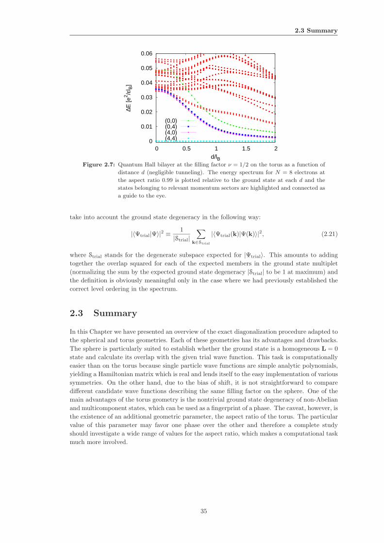
2.3 Summary
0
0.01
0.02
0.03
0.04
0.05
0.06
0 0.5 1 1.5 2
∆E [e
2 /εl B
]
d/lB
(0,0)(0,4)(4,0)(4,4)
Figure 2.7: Quantum Hall bilayer at the filling factor ν = 1/2 on the torus as a function of
distance d (negligible tunneling). The energy spectrum for N = 8 electrons at
the aspect ratio 0.99 is plotted relative to the ground state at each d and the
states belonging to relevant momentum sectors are highlighted and connected as
a guide to the eye.
take into account the ground state degeneracy in the following way:
|〈Ψtrial|Ψ〉|2 ≡1
|Strial|∑
k∈Strial
|〈Ψtrial(k)|Ψ(k)〉|2, (2.21)
where Strial stands for the degenerate subspace expected for |Ψtrial〉. This amounts to adding
together the overlap squared for each of the expected members in the ground state multiplet
(normalizing the sum by the expected ground state degeneracy |Strial| to be 1 at maximum) and
the definition is obviously meaningful only in the case where we had previously established the
correct level ordering in the spectrum.
2.3 Summary
In this Chapter we have presented an overview of the exact diagonalization procedure adapted to
the spherical and torus geometries. Each of these geometries has its advantages and drawbacks.
The sphere is particularly suited to establish whether the ground state is a homogeneous L = 0
state and calculate its overlap with the given trial wave function. This task is computationally
easier than on the torus because single particle wave functions are simple analytic polynomials,
yielding a Hamiltonian matrix which is real and lends itself to the easy implementation of various
symmetries. On the other hand, due to the bias of shift, it is not straightforward to compare
different candidate wave functions describing the same filling factor on the sphere. One of the
main advantages of the torus geometry is the nontrivial ground state degeneracy of non-Abelian
and multicomponent states, which can be used as a fingerprint of a phase. The caveat, however, is
the existence of an additional geometric parameter, the aspect ratio of the torus. The particular
value of this parameter may favor one phase over the other and therefore a complete study
should investigate a wide range of values for the aspect ratio, which makes a computational task
much more involved.
35

2. NUMERICAL STUDIES OF THE FQHE
36
Chapter 3
Quantum disordering of the
quantum Hall bilayer at ν = 1
Quantum Hall bilayer (QHB) at ν = 1 continues to be the subject of many experimental and
theoretical studies. Much of the physics has been well established in the extreme cases when the
distance between layers, d, is (1) much smaller or (2) much larger than the magnetic length lB .
When d ≪ lB , i.e. inter and intra Coulomb interactions are about the same, the good starting
point and description is the Halperin state Ψ111 (1.45). The physics in Ψ111 is of the exciton
binding [10, 89]: an electron in one layer and a correlation hole directly oposite to it, in the
other layer, are in a coherent quantum-mechanical superposition in the manner of the Ψ111 wave
function. This exciton description can be a viewpoint of the phenomenon of superfluidity found
in these systems [93] and is closely connected to the concept of composite bosons (CBs) [48] that
can be used as natural quantum Hall quasiparticles in this system. When d ≫ lB we have the
case of the decoupled layers and the ground state (GS) is a product of two Fermi seas (1.37),
ΨRR(z↑) × ΨRR(z↓). The underlying quasiparticles are then CFs, the usual quasiparticles
of the single layer quantum Hall physics. [1]. To address the range of intermediate d, when
the system is a disordered superfluid, one may try to describe the basic physics by interpolating
between the two limits or, in other words, to construct mixed states of CBs and CFs. [101] This is
a phenomenological approach where we start from the identical electrons, split them into a group
of those that correlate as composite bosons and a group of those that correlate as composite
fermions. The wave function for the superfluid state at small d will involve mainly composite
bosons; the disordering of the CB superfluid is caused by “nucleation” of CF quasiparticles as
d is increased. In this Chapter we study such states using Chern-Simons theory. We begin by
introducing the Chern-Simons approach for the Halperin 111 state, deriving its basic properties
(such as the Goldstone mode and true ODLRO) and pointing out some of its weaknesses (Sec
3.1). We then generalize the theory to the mixed states of CBs and CFs (Sec. 3.2), study their
basic response (Sec. 3.3) and investigate possible phases that these wave functions define as
representatives of the universality classes, on the basis of analytic considerations and numerics
(Sec. 3.4). This Chapter summarizes the main results of Refs. [104] and [105] and presents some
new results of the numerical calculations (Sec. 3.4).
3.1 Chern-Simons theory for the Halperin 111 state
We have introduced the 111 Halperin state in (1.45). Here we show how this wave function can
be obtained as the ground state of a Chern-Simons theory in a particularly transparent way and
derive some of its basic physical properties. These conclusions were previously obtained in more
powerful approaches such as the one in Ref. [92].
37
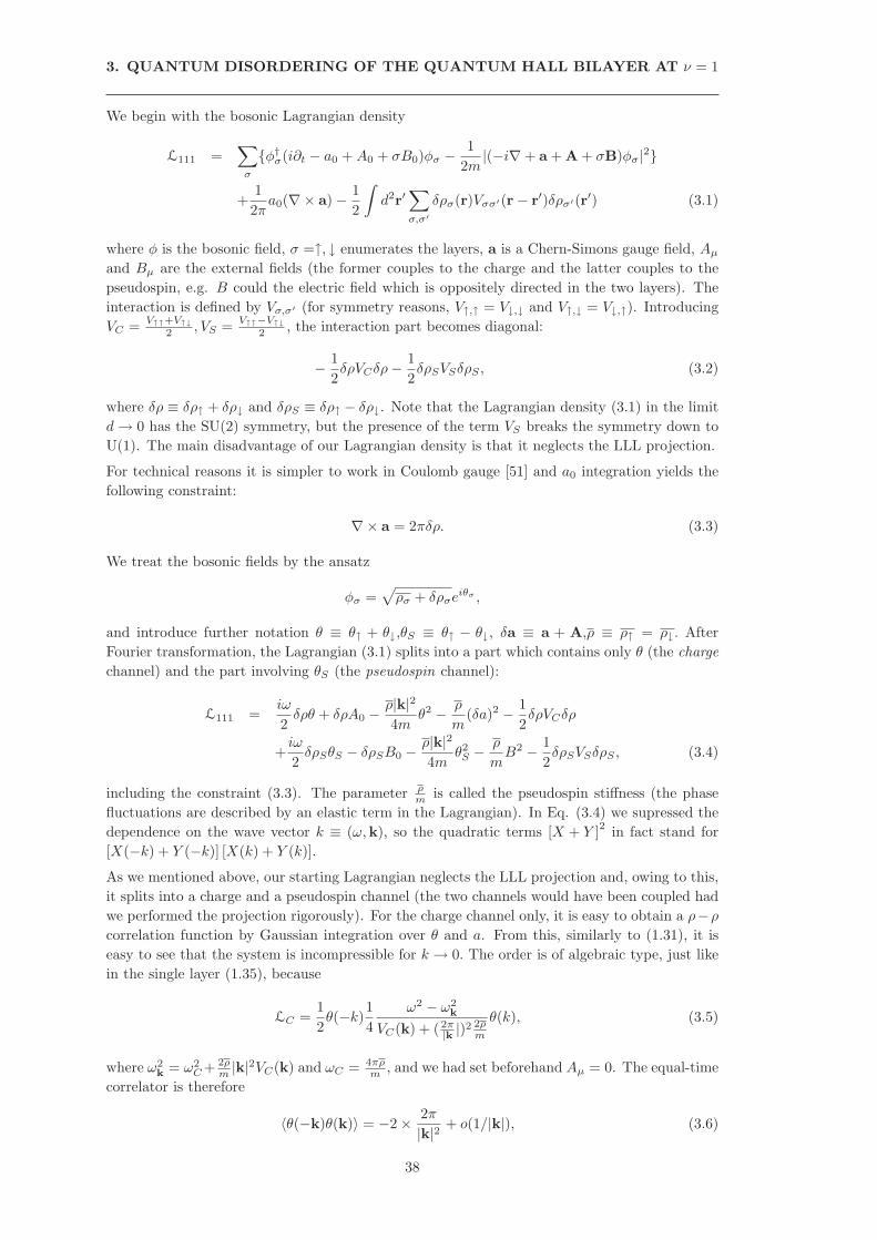
3. QUANTUM DISORDERING OF THE QUANTUM HALL BILAYER AT ν = 1
We begin with the bosonic Lagrangian density
L111 =∑
σ
φ†σ(i∂t − a0 +A0 + σB0)φσ −1
2m|(−i∇+ a + A + σB)φσ|2
+1
2πa0(∇× a)− 1
2
∫
d2r′∑
σ,σ′
δρσ(r)Vσσ′(r− r′)δρσ′(r′) (3.1)
where φ is the bosonic field, σ =↑, ↓ enumerates the layers, a is a Chern-Simons gauge field, Aµ
and Bµ are the external fields (the former couples to the charge and the latter couples to the
pseudospin, e.g. B could the electric field which is oppositely directed in the two layers). The
interaction is defined by Vσ,σ′ (for symmetry reasons, V↑,↑ = V↓,↓ and V↑,↓ = V↓,↑). Introducing
VC =V↑↑+V↑↓
2 , VS =V↑↑−V↑↓
2 , the interaction part becomes diagonal:
− 1
2δρVCδρ−
1
2δρSVSδρS , (3.2)
where δρ ≡ δρ↑ + δρ↓ and δρS ≡ δρ↑ − δρ↓. Note that the Lagrangian density (3.1) in the limit
d→ 0 has the SU(2) symmetry, but the presence of the term VS breaks the symmetry down to
U(1). The main disadvantage of our Lagrangian density is that it neglects the LLL projection.
For technical reasons it is simpler to work in Coulomb gauge [51] and a0 integration yields the
following constraint:
∇× a = 2πδρ. (3.3)
We treat the bosonic fields by the ansatz
φσ =√
ρσ + δρσeiθσ ,
and introduce further notation θ ≡ θ↑ + θ↓,θS ≡ θ↑ − θ↓, δa ≡ a + A,ρ ≡ ρ↑ = ρ↓. After
Fourier transformation, the Lagrangian (3.1) splits into a part which contains only θ (the charge
channel) and the part involving θS (the pseudospin channel):
L111 =iω
2δρθ + δρA0 −
ρ|k|24m
θ2 − ρ
m(δa)2 − 1
2δρVCδρ
+iω
2δρSθS − δρSB0 −
ρ|k|24m
θ2S −ρ
mB2 − 1
2δρSVSδρS , (3.4)
including the constraint (3.3). The parameter ρm is called the pseudospin stiffness (the phase
fluctuations are described by an elastic term in the Lagrangian). In Eq. (3.4) we supressed the
dependence on the wave vector k ≡ (ω,k), so the quadratic terms [X + Y ]2
in fact stand for
[X(−k) + Y (−k)] [X(k) + Y (k)].
As we mentioned above, our starting Lagrangian neglects the LLL projection and, owing to this,
it splits into a charge and a pseudospin channel (the two channels would have been coupled had
we performed the projection rigorously). For the charge channel only, it is easy to obtain a ρ−ρcorrelation function by Gaussian integration over θ and a. From this, similarly to (1.31), it is
easy to see that the system is incompressible for k → 0. The order is of algebraic type, just like
in the single layer (1.35), because
LC =1
2θ(−k)1
4
ω2 − ω2k
VC(k) + (2π|k |)2
2ρm
θ(k), (3.5)
where ω2k = ω2
C + 2ρm |k|2VC(k) and ωC = 4πρ
m , and we had set beforehand Aµ = 0. The equal-time
correlator is therefore
〈θ(−k)θ(k)〉 = −2× 2π
|k|2 + o(1/|k|), (3.6)
38
3.1 Chern-Simons theory for the Halperin 111 state
which is similar to the result for a single layer (1.34), and therefore the ODLRO
lim|r−r′|→∞
〈φ†(r)φ(r′)〉 ∝ 〈ei(θ(r)−θ(r′))〉 ∼ |r− r′|−2, (3.7)
is also algebraic. In the pseudospin channel the situation is more interesting. The effective
Lagrangian in this case is
LS =1
2θS(−k)ω
2 − 2ρmVS(k)|k|24VS(k)
θS(k), (3.8)
assuming that the external field Bµ = 0 to avoid clutter. The correlator is then
〈θS(−k)θS(k)〉 =4VS(k)
ω2 − 2ρmVS(k)|k|2
. (3.9)
From the pole of the correlation function we find the dispersion relation for the pseudospin mode:
ω0(k) =
√
2ρ
mVS(k) · |k|, (3.10)
which is the well-known acoustic mode from the theory of superfluids [51], also derived in Moon
et al. [92]. In the long-wavelength limit we can estimate VS(k) = 12ǫ (
2π|k| − 2π
|k|e−|k|d) ≈ π
ǫ d, plug
in m ≈ 0.07me, ρ ≈ 2.5× 1010cm−2, d/lB = 1.6, ǫ = 12.6, to conclude that the Goldstone mode
obtained from the Chern-Simons theory exceeds the measured value [93] by as much as an order
of magnitude, which illustrates the quantitative weakness of Chern-Simons theory.
The real-space correlation function for θS is
〈θS(r)θS(r′)〉 =1
|r− r′|
√
md
2πǫρ, (3.11)
which leads to the true ODLRO in the pseudospin channel:
〈φ†(r)φ(r′) ∝ lim|r−r′|→∞
e〈θ(r)θ(r′)〉 −→ const. (3.12)
Therefore, in the pseudospin channel, the system is superfluid, compressible and possesses a
linear (acoustic) mode which is the cause of the tunneling resonance in Spielman experiment.
[93]
On the other hand, Halperin’s 111 wave function also naturally follows from the Lagrangian (3.1).
First we focus on the charge channel only. In this channel, θ and δρ are mutually constrained
in a Berry-like term, which implies the commutation relation between them [θ(k), δρ(k′)] =
2iδ(k + k′). The Hamiltonian in the charge sector can be evaluated as [51]
HC =ρ
m
[ |k|24θ(−k)θ(k) + (
2π
|k| )2δρ(−k)δρ(k)
]
+1
2δρ(−k)VC(k)δρ(k). (3.13)
Upon the substitution θ(k)→ −2i ∂∂δρ(−k) , one can recognize the harmonic oscillator Hamiltonian
and the ground state is therefore
Ψgs ∝ exp
[
−1
2
∑
k
2π
|k|2 δρ(−k)δρ(k)
]
. (3.14)
Using δρ(r) =∑
(r − zi↑) +∑
(r − zi↓) − δρ, going to the real space (with some subtleties in
integration, explained in Ref. [51]), we obtain that Ψgs is nothing but the modulus of Halperin’s
111 wave function:
Ψgs = |Ψ111|. (3.15)
39
3. QUANTUM DISORDERING OF THE QUANTUM HALL BILAYER AT ν = 1
Figure 3.1: Universality classes of the wave functions Ψ1 (a) and Ψ2 (b), together with their
paired versions, (c) and (d), respectively.
Thus we have obtained the ground state wave function in the bosonic picture. The original
fermionic wave function can be obtained by an inverse Chern-Simons transformation, which in
this case is given by
U =∏
i<j
zi↑ − zj↑|zi↑ − zj↑|
∏
k<l
zk↓ − zl↓|zk↓ − zl↓|
∏
m,n
zm↑ − zn↓|zm↑ − zn↓|
. (3.16)
Upon acting by U we recover the full 111 wave function: UΨgs = Ψ111. If we take into account
also the pseudospin channel, it can be shown [51] that its contribution is a simple constant
for d = 0. For d nonzero, and especially towards d ∼ lB , the system experiences quantum
fluctuations and its ground state begins to show significant deviations from the 111 state.
3.2 Trial wave functions for the quantum Hall bilayer
In the previous Section we have seen that the 111 state provides a description of the quantum
Hall bilayer for d = 0 and perhaps small nonzero d’s. As d is increased towards d ∼ lB , the
quantum fluctuations grow strong and the superfluid undergoes disordering. To describe the
intermediate distances, we may try to, classically speaking, divide electrons into two groups,
one in which the electrons are correlated as CBs and the other as CFs. [101] The ratio between
the numbers of CBs and CFs would be determined by the distance between layers. The wave
function constructed in this way would need an overall antisymmetrization in the end, but also
intercorrelations among the groups as each electron of the system “sees” the same number of flux
quanta through the system (equal to the number of electrons). This requires that the highest
power of any electron coordinate is the same as the number of electrons in the thermodynamic
limit. If we denote by a line the Laughlin-Jastrow factor∏
A,B(zA−zB) between the two groups
of electrons, A and B (A,B = CB,CF ), the possibilities for the QHB wave functions can be
summarized as in Fig. 3.1.
If we ignore the possibility of pairing between CFs, [145] denoted by wriggly lines in Fig. 3.1(c)
and Fig. 3.1(d), we have two basic families of the wave functions depicted in Fig. 3.1(a) and
Fig. 3.1(b). The requirement that each electron “sees” the same number of flux quanta through
the system equal to the number of electrons (as we are at ν = 1) very much reduces the number
of possible wave functions in the mixed CB - CF approach. We can consider, for example, the
40
3.2 Trial wave functions for the quantum Hall bilayer
possibility depicted in Fig. 3.1(a) which stands for the following wave-function in the LLL,
Ψ1 = PLLLA↑A↓
∏
i<j
(zi↑ − zj↑)∏
k<l
(zk↓ − zl↓)∏
p,q
(zp↑ − zq↓)
×F(w↑, w↑)∏
i<j
(wi↑ − wj↑)2 × F(w↓, w↓)
∏
k<l
(wk↓ − wl↓)2
×∏
i,j
(zi↑ − wj↑)∏
k,l
(zk↑ − wl↓)∏
p,q
(zp,↓ − wq,↑)∏
m,n
(zm↓ − wn↓)
, (3.17)
where A↑ and A↓ denote the overall antisymmetrizations, ziσ are the coordinates of CBs in the
layer σ =↑, ↓ and wiσ are the coordinates of CFs in the layer σ. In the thermodynamic limit,
the relation between the number of particles and flux quanta reads,
N bφ = Nb↑ +Nb↓ +Nf↑ +Nf↓,
Nf↑φ = 2Nf↑ +Nb↑ +Nb↓,
Nf↓φ = 2Nf↓ +Nb↑ +Nb↓, (3.18)
where we denoted by N bφ and Nfσ
φ separately the number of flux quanta which electrons that
correlate as CBs and CFs respectively see, Nbσ and Nfσ are the number of CBs and CFs inside
the layer σ, respectively. The requirement constrains Nφ = N bφ = Nfσ
φ , where Nφ is the number
of flux quanta through the system. This leads to the additional requirement Nf↑ = Nf↓ which
leaves Nb↑ − Nb↓ unconstrained, connected with the Bose condensation phenomenon that this
wave function should be part of [10, 89, 92, 104].
The only additional way to introduce the correlations among the electrons is as follows:
Ψ2 = PLLLA↑A↓
∏
i<j
(zi↑ − zj↑)∏
k<l
(zk↓ − zl↓)∏
p,q
(zp↑ − zq↓)
×F(w↑, w↑)∏
i<j
(wi↑ − wj↑)2 × F(w↓, w↓)
∏
k<l
(wk↓ − wl↓)2
×∏
i,j
(zi↑ − wj↑)2∏
k,l
(zk↓ − wl↓)2
. (3.19)
This wave function is depicted in Fig. 3.1(b). Whereas the intercorrelations in the first family
in Fig. 3.1(a) are in the spirit of Ψ111 correlations, those in the second family in Fig. 3.1(b),
represented by Ψ2, are in the spirit of the decoupled states, ΨRR × ΨRR, where we correlate
exclusively inside each layer. In this case the flux-counting reads:
N b↑φ = Nb↑ +Nb↓ + 2Nf↑,
N b↓φ = Nb↑ +Nb↓ + 2Nf↓,
Nf↑φ = 2Nf↑ + 2Nb↑,
Nf↓φ = 2Nf↓ + 2Nb↓, (3.20)
which leads to the constraints Nb↑ = Nb↓ and Nf↑ = Nf↓.
We can imagine a mixture of both intercorrelations (of Fig. 3.1(a) and Fig. 3.1(b)) in a single
wave function but these mixed states, by their basic response [104], fall into one of the universality
classes depicted in Fig. 3.1. In Sec. 3.4 we will explicitly consider these possibilities and prove,
in the scope of a CS theory, that the case Fig. 3.1(b) does not support a Goldstone (gapless)
mode which exists for the state depicted in Fig. 3.1(a). These generalized states therefore belong
to the universality class of the state depicted in Fig. 3.1(b) for which in the scope of CS theory
we find in the low-energy spectrum only a gapped collective mode.[104]
41
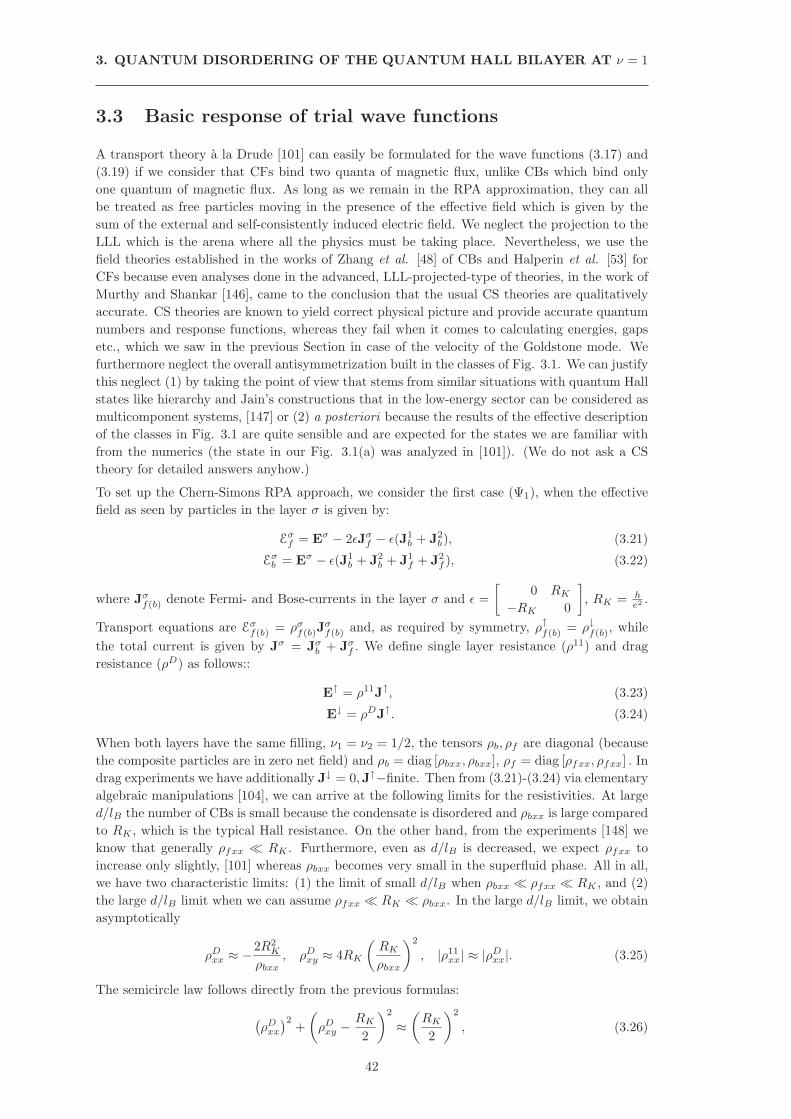
3. QUANTUM DISORDERING OF THE QUANTUM HALL BILAYER AT ν = 1
3.3 Basic response of trial wave functions
A transport theory a la Drude [101] can easily be formulated for the wave functions (3.17) and
(3.19) if we consider that CFs bind two quanta of magnetic flux, unlike CBs which bind only
one quantum of magnetic flux. As long as we remain in the RPA approximation, they can all
be treated as free particles moving in the presence of the effective field which is given by the
sum of the external and self-consistently induced electric field. We neglect the projection to the
LLL which is the arena where all the physics must be taking place. Nevertheless, we use the
field theories established in the works of Zhang et al. [48] of CBs and Halperin et al. [53] for
CFs because even analyses done in the advanced, LLL-projected-type of theories, in the work of
Murthy and Shankar [146], came to the conclusion that the usual CS theories are qualitatively
accurate. CS theories are known to yield correct physical picture and provide accurate quantum
numbers and response functions, whereas they fail when it comes to calculating energies, gaps
etc., which we saw in the previous Section in case of the velocity of the Goldstone mode. We
furthermore neglect the overall antisymmetrization built in the classes of Fig. 3.1. We can justify
this neglect (1) by taking the point of view that stems from similar situations with quantum Hall
states like hierarchy and Jain’s constructions that in the low-energy sector can be considered as
multicomponent systems, [147] or (2) a posteriori because the results of the effective description
of the classes in Fig. 3.1 are quite sensible and are expected for the states we are familiar with
from the numerics (the state in our Fig. 3.1(a) was analyzed in [101]). (We do not ask a CS
theory for detailed answers anyhow.)
To set up the Chern-Simons RPA approach, we consider the first case (Ψ1), when the effective
field as seen by particles in the layer σ is given by:
Eσf = Eσ − 2ǫJσ
f − ǫ(J1b + J2
b), (3.21)
Eσb = Eσ − ǫ(J1
b + J2b + J1
f + J2f ), (3.22)
where Jσf(b) denote Fermi- and Bose-currents in the layer σ and ǫ =
[
0 RK
−RK 0
]
, RK = he2 .
Transport equations are Eσf(b) = ρσ
f(b)Jσf(b) and, as required by symmetry, ρ↑f(b) = ρ↓f(b), while
the total current is given by Jσ = Jσb + Jσ
f . We define single layer resistance (ρ11) and drag
resistance (ρD) as follows::
E↑ = ρ11J↑, (3.23)
E↓ = ρDJ↑. (3.24)
When both layers have the same filling, ν1 = ν2 = 1/2, the tensors ρb, ρf are diagonal (because
the composite particles are in zero net field) and ρb = diag [ρbxx, ρbxx], ρf = diag [ρfxx, ρfxx] . In
drag experiments we have additionally J↓ = 0,J↑−finite. Then from (3.21)-(3.24) via elementary
algebraic manipulations [104], we can arrive at the following limits for the resistivities. At large
d/lB the number of CBs is small because the condensate is disordered and ρbxx is large compared
to RK , which is the typical Hall resistance. On the other hand, from the experiments [148] we
know that generally ρfxx ≪ RK . Furthermore, even as d/lB is decreased, we expect ρfxx to
increase only slightly, [101] whereas ρbxx becomes very small in the superfluid phase. All in all,
we have two characteristic limits: (1) the limit of small d/lB when ρbxx ≪ ρfxx ≪ RK , and (2)
the large d/lB limit when we can assume ρfxx ≪ RK ≪ ρbxx. In the large d/lB limit, we obtain
asymptotically
ρDxx ≈ −
2R2K
ρbxx, ρD
xy ≈ 4RK
(
RK
ρbxx
)2
, |ρ11xx| ≈ |ρD
xx|. (3.25)
The semicircle law follows directly from the previous formulas:
(
ρDxx
)2+
(
ρDxy −
RK
2
)2
≈(
RK
2
)2
, (3.26)
42
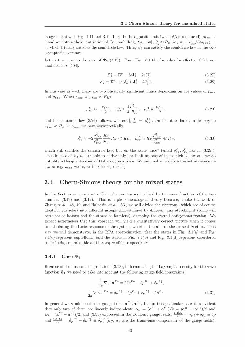
3.4 Chern-Simons theory for the mixed states
in agreement with Fig. 1.11 and Ref. [149]. In the opposite limit (when d/lB is reduced), ρbxx →0 and we obtain the quantization of Coulomb drag, [94, 150] ρD
xy ≈ RK , ρDxx ≈ −ρ2
bxx/(2ρfxx)→0, which trivially satisfies the semicircle law. Thus, Ψ1 can satisfy the semicircle law in the two
asymptotic extremes.
Let us turn now to the case of Ψ2 (3.19). From Fig. 3.1 the formulas for effective fields are
modified into [104]:
Eσf = Eσ − 2ǫJσ
f − 2ǫJσb , (3.27)
Eσb = Eσ − ǫ(J1
b + J2b + 2Jσ
f ). (3.28)
In this case as well, there are two physically significant limits depending on the values of ρbxx
and ρfxx. When ρbxx ≪ ρfxx ≪ RK :
ρDxx ≈ −
ρfxx
2, ρD
xy ≈1
4
ρ2fxx
RK, ρ11
xx ≈ρfxx
2, (3.29)
and the semicircle law (3.26) follows, whereas |ρDxx| = |ρ11
xx|. On the other hand, in the regime
ρfxx ≪ RK ≪ ρbxx, we have asymptotically
ρDxx ≈ −2
ρ2fxx
ρ2bxx
RK
ρbxxRK ≪ RK , ρD
xy ≈ RK
ρ2fxx
ρ2bxx
≪ RK , (3.30)
which still satisfies the semicircle law, but on the same “side” (small ρDxx, ρ
Dxy like in (3.29)).
Thus in case of Ψ2 we are able to derive only one limiting case of the semicircle law and we do
not obtain the quantization of Hall drag resistance. We are unable to derive the entire semicircle
law as e.g. ρbxx varies, neither for Ψ1 nor Ψ2.
3.4 Chern-Simons theory for the mixed states
In this Section we construct a Chern-Simons theory inspired by the wave functions of the two
families, (3.17) and (3.19). This is a phenomenological theory because, unlike the work of
Zhang et al. [48, 49] and Halperin et al. [53], we will divide the electrons (which are of course
identical particles) into different groups characterized by different flux attachment (some will
correlate as bosons and the others as fermions), dropping the overall antisymmetrization. We
expect nonetheless that this approach will yield a qualitatively correct picture when it comes
to calculating the basic response of the system, which is the aim of the present Section. This
way we will demonstrate, in the RPA approximation, that the states in Fig. 3.1(a) and Fig.
3.1(c) represent superfluids, and the states in Fig. 3.1(b) and Fig. 3.1(d) represent disordered
superfluids, compressible and incompressible, respectively.
3.4.1 Case Ψ1
Because of the flux counting relations (3.18), in formulating the Lagrangian density for the wave
function Ψ1 we need to take into account the following gauge field constraints:
1
2π∇× aFσ = 2δρFσ + δρB↑ + δρB↓,
1
2π∇× aBσ = δρF↑ + δρF↓ + δρB↑ + δρB↓. (3.31)
In general we would need four gauge fields aFσ,aBσ, but in this particular case it is evident
that only two of them are linearly independent: aC = (aF↑ + aF↓)/2 = (aB↑ + aB↓)/2 and
aS = (aF↑ − aF↓)/2, and (3.31) expressed in the Coulomb gauge reads: i|k|aC
2π = δρ↑ + δρ↓ ≡ δρand i|k|aS
2π = δρF↑ − δρF↓ ≡ δρFS (aC , aS are the transverse components of the gauge fields).
43
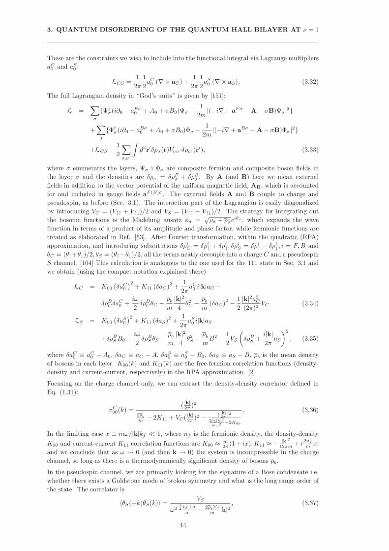
3. QUANTUM DISORDERING OF THE QUANTUM HALL BILAYER AT ν = 1
These are the constraints we wish to include into the functional integral via Lagrange multipliers
aC0 and aS
0 :
LCS =1
2π
1
2aC0 (∇× aC) +
1
2π
1
2aS0 (∇× aS) . (3.32)
The full Lagrangian density in “God’s units” is given by [151]:
L =∑
σ
Ψ†σ(i∂0 − aFσ
0 +A0 + σB0)Ψσ −1
2m|(−i∇+ aFσ −A− σB)Ψσ|2
+∑
σ
Φ†σ(i∂0 − aBσ
0 +A0 + σB0)Φσ −1
2m|(−i∇+ aBσ −A− σB)Φσ|2
+LCS −1
2
∑
σ,σ′
∫
d2r′δρσ(r)Vσσ′δρσ′(r′), (3.33)
where σ enumerates the layers, Ψσ i Φσ are composite fermion and composite boson fields in
the layer σ and the densities are δρσ = δρFσ + δρB
σ . By A (and B) here we mean external
fields in addition to the vector potential of the uniform magnetic field, AB, which is accounted
for and included in gauge fields aF (B)σ. The external fields A and B couple to charge and
pseudospin, as before (Sec. 3.1). The interaction part of the Lagrangian is easily diagonalized
by introducing VC = (V↑↑ + V↑↓)/2 and VS = (V↑↑ − V↑↓)/2. The strategy for integrating out
the bosonic functions is the Madelung ansatz φσ =√ρσ + ρσe
iθσ , which expands the wave
function in terms of a product of its amplitude and phase factor, while fermionic functions are
treated as elaborated in Ref. [53]. After Fourier transformation, within the quadratic (RPA)
approximation, and introducing substitutions δρiC = δρi
↑ + δρi↓, δρ
iS = δρi
↑ − δρi↓, i = F,B and
θC = (θ↑+θ↓)/2, θS = (θ↑−θ↓)/2, all the terms neatly decouple into a charge C and a pseudospin
S channel. [104] This calculation is analogous to the one used for the 111 state in Sec. 3.1 and
we obtain (using the compact notation explained there)
LC = K00
(
δaC0
)2+K11 (δaC)
2+
1
2πaC0 i|k|aC −
δρBCδa
C0 +
iω
2δρB
CθC −ρb
m
|k|24θ2C −
ρb
m(δaC)
2 − 1
2
|k|2a2C
(2π)2VC (3.34)
LS = K00
(
δaS0
)2+K11 (δaS)
2+
1
2πaS0 i|k|aS
+δρBSB0 +
iω
2δρB
S θS −ρb
m
|k|24θ2S −
ρb
mB2 − 1
2VS
(
δρBS +
i|k|2π
aS
)2
, (3.35)
where δaC0 ≡ aC
0 − A0, δaC ≡ aC − A, δaS0 ≡ aS
0 − B0, δaS ≡ aS − B, ρb is the mean density
of bosons in each layer. K00(k) and K11(k) are the free-fermion correlation functions (density-
density and current-current, respectively) in the RPA approximation. [2]
Focusing on the charge channel only, we can extract the density-density correlator defined in
Eq. (1.31):
πC00(k) =
( |k|2π )2
2ρb
m − 2K11 + VC( |k|2π )2 − (|k|2π
)2
2ρb|k|2
mω2 −2K00
. (3.36)
In the limiting case x ≡ mω/|k|kf ≪ 1, where nf is the fermionic density, the density-density
K00 and current-current K11 correlation functions are K00 ≈ m2π (1 + ix),K11 ≈ − |k|2
12πm + i2nf
m x,
and we conclude that as ω → 0 (and then k → 0) the system is incompressible in the charge
channel, so long as there is a thermodynamically significant density of bosons ρb.
In the pseudospin channel, we are primarily looking for the signature of a Bose condensate i.e.
whether there exists a Goldstone mode of broken symmetry and what is the long range order of
the state. The correlator is
〈θS(−k)θS(k)〉 =VS
ω212VS+α
α − 2ρbVS
m |k|2, (3.37)
44
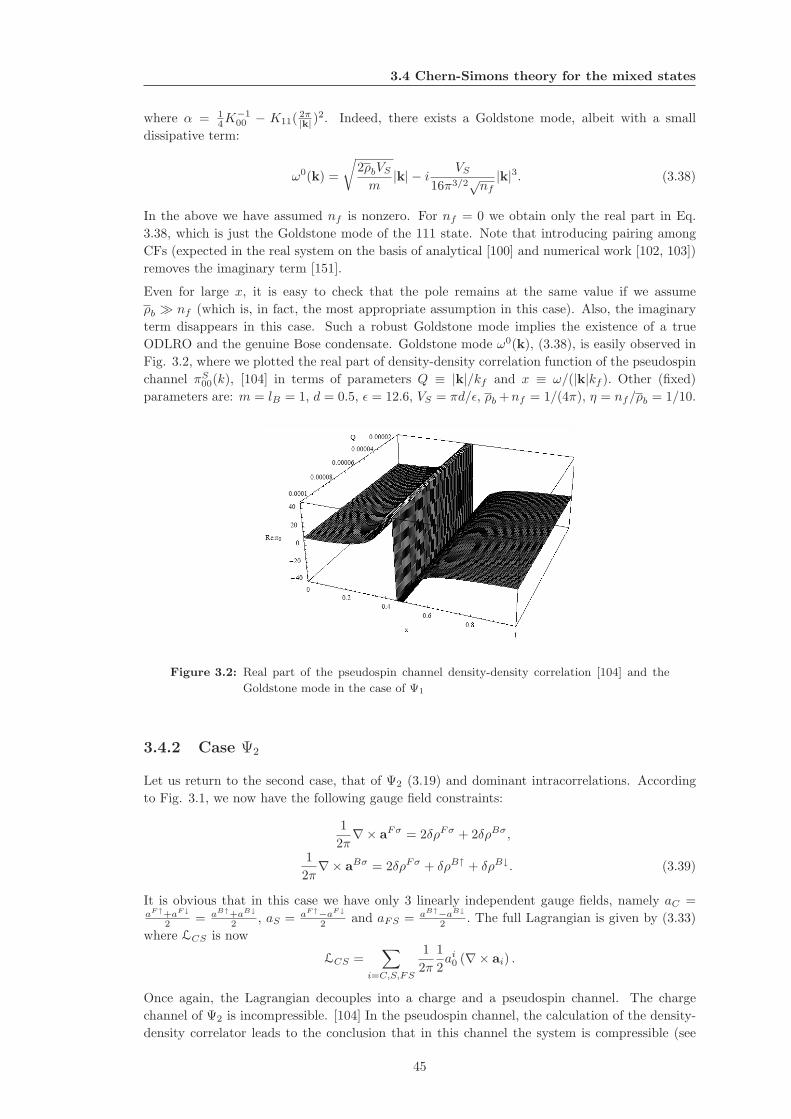
3.4 Chern-Simons theory for the mixed states
where α = 14K
−100 − K11(
2π|k| )
2. Indeed, there exists a Goldstone mode, albeit with a small
dissipative term:
ω0(k) =
√
2ρbVS
m|k| − i VS
16π3/2√nf|k|3. (3.38)
In the above we have assumed nf is nonzero. For nf = 0 we obtain only the real part in Eq.
3.38, which is just the Goldstone mode of the 111 state. Note that introducing pairing among
CFs (expected in the real system on the basis of analytical [100] and numerical work [102, 103])
removes the imaginary term [151].
Even for large x, it is easy to check that the pole remains at the same value if we assume
ρb ≫ nf (which is, in fact, the most appropriate assumption in this case). Also, the imaginary
term disappears in this case. Such a robust Goldstone mode implies the existence of a true
ODLRO and the genuine Bose condensate. Goldstone mode ω0(k), (3.38), is easily observed in
Fig. 3.2, where we plotted the real part of density-density correlation function of the pseudospin
channel πS00(k), [104] in terms of parameters Q ≡ |k|/kf and x ≡ ω/(|k|kf ). Other (fixed)
parameters are: m = lB = 1, d = 0.5, ǫ = 12.6, VS = πd/ǫ, ρb +nf = 1/(4π), η = nf/ρb = 1/10.
Figure 3.2: Real part of the pseudospin channel density-density correlation [104] and the
Goldstone mode in the case of Ψ1
3.4.2 Case Ψ2
Let us return to the second case, that of Ψ2 (3.19) and dominant intracorrelations. According
to Fig. 3.1, we now have the following gauge field constraints:
1
2π∇× aFσ = 2δρFσ + 2δρBσ,
1
2π∇× aBσ = 2δρFσ + δρB↑ + δρB↓. (3.39)
It is obvious that in this case we have only 3 linearly independent gauge fields, namely aC =aF↑+aF↓
2 = aB↑+aB↓
2 , aS = aF↑−aF↓
2 and aFS = aB↑−aB↓
2 . The full Lagrangian is given by (3.33)
where LCS is now
LCS =∑
i=C,S,FS
1
2π
1
2ai0 (∇× ai) .
Once again, the Lagrangian decouples into a charge and a pseudospin channel. The charge
channel of Ψ2 is incompressible. [104] In the pseudospin channel, the calculation of the density-
density correlator leads to the conclusion that in this channel the system is compressible (see
45
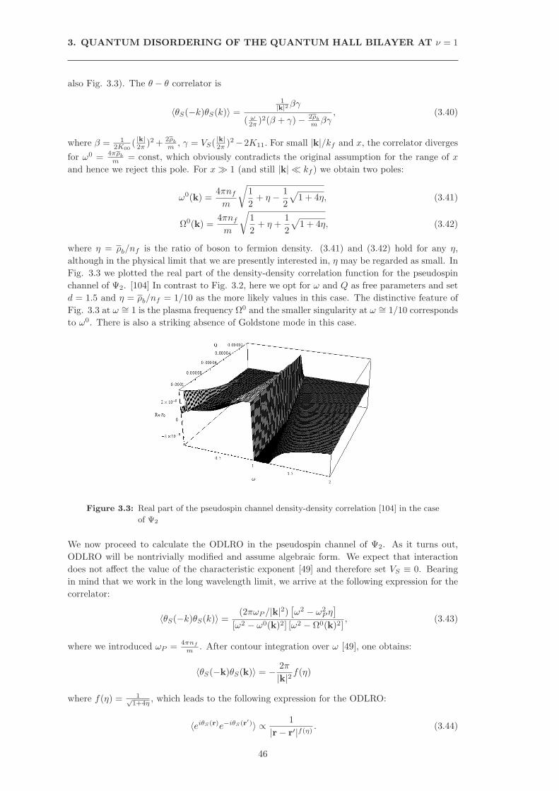
3. QUANTUM DISORDERING OF THE QUANTUM HALL BILAYER AT ν = 1
also Fig. 3.3). The θ − θ correlator is
〈θS(−k)θS(k)〉 =
1|k|2 βγ
( ω2π )2(β + γ)− 2ρb
m βγ, (3.40)
where β = 12K00
( |k|2π )2 + 2ρb
m , γ = VS( |k|2π )2−2K11. For small |k|/kf and x, the correlator diverges
for ω0 = 4πρb
m = const, which obviously contradicts the original assumption for the range of x
and hence we reject this pole. For x≫ 1 (and still |k| ≪ kf ) we obtain two poles:
ω0(k) =4πnf
m
√
1
2+ η − 1
2
√
1 + 4η, (3.41)
Ω0(k) =4πnf
m
√
1
2+ η +
1
2
√
1 + 4η, (3.42)
where η = ρb/nf is the ratio of boson to fermion density. (3.41) and (3.42) hold for any η,
although in the physical limit that we are presently interested in, η may be regarded as small. In
Fig. 3.3 we plotted the real part of the density-density correlation function for the pseudospin
channel of Ψ2. [104] In contrast to Fig. 3.2, here we opt for ω and Q as free parameters and set
d = 1.5 and η = ρb/nf = 1/10 as the more likely values in this case. The distinctive feature of
Fig. 3.3 at ω ∼= 1 is the plasma frequency Ω0 and the smaller singularity at ω ∼= 1/10 corresponds
to ω0. There is also a striking absence of Goldstone mode in this case.
Figure 3.3: Real part of the pseudospin channel density-density correlation [104] in the case
of Ψ2
We now proceed to calculate the ODLRO in the pseudospin channel of Ψ2. As it turns out,
ODLRO will be nontrivially modified and assume algebraic form. We expect that interaction
does not affect the value of the characteristic exponent [49] and therefore set VS ≡ 0. Bearing
in mind that we work in the long wavelength limit, we arrive at the following expression for the
correlator:
〈θS(−k)θS(k)〉 =(2πωP /|k|2)
[
ω2 − ω2P η]
[ω2 − ω0(k)2] [ω2 − Ω0(k)2], (3.43)
where we introduced ωP =4πnf
m . After contour integration over ω [49], one obtains:
〈θS(−k)θS(k)〉 = − 2π
|k|2 f(η)
where f(η) = 1√1+4η
, which leads to the following expression for the ODLRO:
〈eiθS(r)e−iθS(r′)〉 ∝ 1
|r− r′|f(η). (3.44)
46
3.5 Possibility for a paired intermediate phase in the bilayer
For η →∞ when there are no CFs, the correlator (3.44) is a constant. However, Ψ2 is expected
to represent the system when η is small. In that case, even at T = 0, we obtain the algebraic
ODLRO
〈eiθS(r)e−iθS(r′)〉 ≈ |r− r′|−(1−2η+o(η2)),
which indicates that Ψ2 represents a disordered fluid, although possibly with some remaining
intercorrelation.
3.4.3 Generalized states
We can imagine that, apart from Ψ1 and Ψ2, we may have a state that contains a combination
of both. We can analyze the response of the state which, in addition to Ψ2, includes (in each
layer) a different kind of CFs that connect to the CB in the manner of Ψ1. This gives us the
following gauge field constraints:
1
2π∇× aBσ = δρB↑ + δρB↓ + δρ
(1)F↑ + δρ
(1)F↓ + 2δρ
(2)Fσ, (3.45)
1
2π∇× aFσ
1 = δρB↑ + δρB↓ + 2δρ(1)Fσ + 2δρ
(2)Fσ, (3.46)
1
2π∇× aFσ
2 = 2δρBσ + 2δρ(1)Fσ + 2δρ
(2)Fσ, (3.47)
where the superscripts (1), (2) indicate CF species in each layer. CS theory easily follows from
the above gauge field equations and yields incompressible behavior in the charge channel. In the
pseudospin channel [104] we can derive the following correlation function:
〈θS(−k)θS(k)〉 =VS +
2nf2
m ( 2π|k| )
2
ω2 − ( 2ρbVS
m |k|2 + (4πm )2ρbnf2)
(3.48)
to see that the low-energy spectrum is dominated by the plasma frequency:
ω0(k) =4π
m
√
ρbnf2, (3.49)
where nf2 is the density of the CFs which bind exclusively within the layer they belong to. We
conclude that the mixed state fall into the universality class of Ψ2.
3.5 Possibility for a paired intermediate phase in the bi-
layer
The classes of wave functions (3.17) and (3.19) (and their paired versions) represent possible
outcomes of superfluid disordering in the quantum Hall bilayer before the system is in the phase
of decoupled Fermi liquids. We now explain how these wave functions generalize the concept of
superfluid disordering of the more traditional theories for small d/lB (Sec. 3.5.1). The connection
will be established on the basis of the predicted first-order (phonon) correction to the 111 state,
which is expected to be universal at small d/lB . In doing so, we identify a simple possibility
for the pairing function at small d/lB in our mixed state approach. Furthermore, a question
can be asked whether, for larger d ∼ lB , the superfluid disordering in the bilayer can lead to an
intermediary paired phase before the layers decouple and each forms a CF liquid. We discuss
this question in Sec. 3.5.2 where we present one of the many candidate wave functions for such
a phase. This wave function is singled out because it incorporates a pairing with the same
angular momentum as the one we derived for small d/lB (this form of pairing is also supported
by numerical studies [102, 103]), but we argue that the phase it describes is likely compressible.
We conclude by showing several numerical results for the transition which give some support to
the scenario of a direct transition between the 111 phase and the CFL (Sec. 3.5.3).
47
3. QUANTUM DISORDERING OF THE QUANTUM HALL BILAYER AT ν = 1
3.5.1 First-order corrections to the 111 state
As we mentioned, for small d/lB we expect our construction Ψ1 to yield the same first-order
correction to the 111 state as the other theories that evaluated this correction from the phonon
contribution. As we start from the small d/lB limit, the physical interpretation of the correction
in our approach is the inclusion of CFs into the CB condensate.
The traditional [49] CS field theory in the RPA approximation [152] of the bilayer problem at
ν = 1 (which in the neutral channel reduces just to the problem of an ordinary superfluid with
the phonon contribution) finds the following correction to the Ψ111 state [153]:
Ψph = exp
− 1
2
∑
k
√
VS(k)ρ/m
|k| ρSkρ
S−k
Ψ111 (3.50)
where ρSk ≡ ρ
↑k − ρ
↓k, VS(k) is the interaction in the neutral channel, m is the electron mass and
ρ is the uniform total density. The form of the correction in the pseudospin sector in Eq.(3.50)
is easily derived along the same lines as in the case of Ψ111, which belongs to the charge sector,
in Eqs.(3.13,3.14). In the small d limit VS(k) = πd and we can expand the expression Ψph as
Ψph = Ψ111 −(
∑
k
c√d
|k| ρS−kρ
Sk
)
Ψ111 + · · · (3.51)
where c is a positive constant. The terms after the first one represent corrections, in the order
of importance, to the Ψ111 ansatz as d increases. The form of the correction is fixed by the basic
phenomenology and sum rules for a superluid in two dimensions. [154]
To show how the wave function Ψ1 (3.17) generalizes the expansion (3.51), let us rewrite the
unprojected wave function Ψ1 in the following way:
Ψ1 = A↑A↓
Ψ111(z↑, z↓)ΨRR(w↑)ΨRR(w↓)∏
i,j
(zi↑ − wj↑)∏
k,l
(zk↑ − wl↓)∏
p,q
(zi↓ − wq↑)∏
m,n
(zm↓ − wn↓)
, (3.52)
where, as before, zσ’s and wσ’s denote coordinates of the electrons belonging to the layer with
index σ and A↑ and A↓, as before, stand for the antisymmetrizations. ΨRR was defined in (1.37).
Using S↑ and S↓, symmetrizers inside each layer, the same function, Ψ1, can be written as:
Ψ1 = S↑S↓
∏
k<l(wk↑ − wl↑)∏
p<q(wp↓ − wq↓)∏
i,j(wi↑ − wj↓)F(w↑)F(w↓)
Ψ111
where Ψ111 denotes the Vandermonde determinant (Slater determinant in the LLL) of all co-
ordinates in which all groups equally participate. By using the expressions for the densities of
electrons in each layer, ρσ(η) =∑
i δ2(η−zσ
i )+∑
i δ2(η−wσ
i ), we can rewrite the wave function
in the following way,
Ψ1 =
∫
d2η1↑ · · ·∫
d2ηn↓
∏
k<l(ηk↑ − ηl↑)∏
p<q(ηp↓ − ηq↓)∏
i,j(ηi↑ − ηj↓)
F(η↑)× F(η↓)× ρ↑(η1↑) · · · ρ↓(ηn↓)Ψ111(z↑, z↓)
, (3.53)
where n is the total number of electrons that correlate as CFs. The equality is exact; any time
we have in the product of ρ’s the same layer electron coordinate more than once, the Laughlin -
Jastrow factors of η’s in the same layer force the wave function to become zero. This expression
reminds us of a dual picture in terms of some quasiparticles with η coordinates as in [33]. It can
be shown that these quasiparticles have to be fermionic. [105]
Now, by virtue of (3.53), we can see that the wave functions of Fig. 3.1(c) allow for the corrections
to the 111 state which are more general than the one used in the expansion (3.51), the only
48
3.5 Possibility for a paired intermediate phase in the bilayer
g(z) = const (no pairing)∑
k f1(d)1
(kx+iky)ρ↑kρ
↓−k
g(z) = 1/z no correction when multiplies Ψ111
g(z) =√
z/z∑
k f2(d)1|k|ρ
↑kρ
↓−k
g(z) = 1/z∑
k f3(d) ln(|k|lB)ρ↑kρ↓−k
Table 3.1: Phonon correction for different choices of the pairing function. The func-
tions f1, f2, and f3 define the weight of each correction in terms of the bi-
layer distance d. In the first case (no pairing) the correction is proportional toP
k
1(kx+iky)
ρ↑
kρ↓
−k, but we expect that with no constraint on the number of CFs
(as in Eqs.(3.50) and (3.51); see also discussion below Eq.(3.53)), this will cor-
respond toP
k
1(kx+iky)
ρSkρS
−k i.e. zero (no correction) due to the antisymmetry
under k → −k exchange.
constraint we need to satisfy is the equal number of ρ↑k’s and ρ↓k’s because in writing down the
classes of Fig. 3.1 we explicitly distinguished ↑’s from ↓’s and fixed the number of ↑’s and ↓’s to
be equal.
Let us compare the first phonon corrections in both approaches to find out which possibilities
for pairing are allowed among the most simple choices for the weak pairing function. From the
usual CS theory, the first phonon correction is ∼ ∑k1|k|ρ
↑−kρ
↓k. On the other hand, the mixed
wave function in Fig. 3.1(c) suggests the following simplest correction for two CFs:
∫
d2η1↑
∫
d2η2↓1
(η1↑ − η2↓)g(η1↑ − η2↓)ρ↑(η1↑)ρ↓(η2↓), (3.54)
where g is the pairing function. If we take the “obvious” choice g(z) = 1/z, we do not obtain
any correction. This is because we need to evaluate
∫
d2η1↑
∫
d2η2↓1
(η1↑ − η2↓)2ρ↑(η1↑)ρ
↓(η2↓), (3.55)
which, after switching to center of mass/relative coordinate, reduces to solving the following
Fourier transform∫
d2η1
η2expik · η. (3.56)
This can be evaluated analytically [105] to find that it does not depend on k:
∫
d2η1
η2expik · η = −π. (3.57)
Therefore the correction in this case is proportional to
(
∑
k
ρ↑kρ↓−k
)
Ψ111, (3.58)
and in real (coordinate) space this becomes:
∫
d2η ρ↑(η)ρ↓(η)Ψ111 =∑
i,j
∫
d2η δ2(η − zi↑)δ2(η − zj↓)Ψ111
=∑
i,j
δ2(zi↑ − zj↓)Ψ111 = 0, (3.59)
i.e. no correction at all.
Taking the next choice g(z) =√
z/z (z is the complex conjugate of z), the expression in Eq.(3.54)
reduces to the form of the first phonon contribution in the long-distance limit with the 1|k|
singularity, (3.51). Thus g(z) =√
z/z accommodates the usual (on the level of RPA) superfluid
description given in (3.51), which which can lead also to a pseudospin density wave. [152]
49
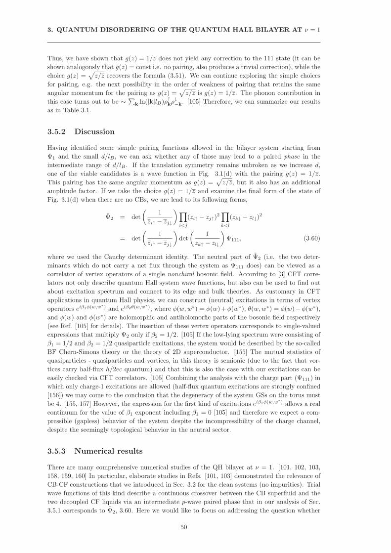
3. QUANTUM DISORDERING OF THE QUANTUM HALL BILAYER AT ν = 1
Thus, we have shown that g(z) = 1/z does not yield any correction to the 111 state (it can be
shown analogously that g(z) = const i.e. no pairing, also produces a trivial correction), while the
choice g(z) =√
z/z recovers the formula (3.51). We can continue exploring the simple choices
for pairing, e.g. the next possibility in the order of weakness of pairing that retains the same
angular momentum for the pairing as g(z) =√
z/z is g(z) = 1/z. The phonon contribution in
this case turns out to be ∼ ∑k ln(|k|lB)ρ↑kρ↓−k. [105] Therefore, we can summarize our results
as in Table 3.1.
3.5.2 Discussion
Having identified some simple pairing functions allowed in the bilayer system starting from
Ψ1 and the small d/lB , we can ask whether any of those may lead to a paired phase in the
intermediate range of d/lB . If the translation symmetry remains unbroken as we increase d,
one of the viable candidates is a wave function in Fig. 3.1(d) with the pairing g(z) = 1/z.
This pairing has the same angular momentum as g(z) =√
z/z, but it also has an additional
amplitude factor. If we take the choice g(z) = 1/z and examine the final form of the state of
Fig. 3.1(d) when there are no CBs, we are lead to its following forms,
Ψ2 = det
(
1
zi↑ − zj↓
)
∏
i<j
(zi↑ − zj↑)2∏
k<l
(zk↓ − zl↓)2
= det
(
1
zi↑ − zj↓
)
det
(
1
zk↑ − zl↓
)
Ψ111, (3.60)
where we used the Cauchy determinant identity. The neutral part of Ψ2 (i.e. the two deter-
minants which do not carry a net flux through the system as Ψ111 does) can be viewed as a
correlator of vertex operators of a single nonchiral bosonic field. According to [3] CFT corre-
lators not only describe quantum Hall system wave functions, but also can be used to find out
about excitation spectrum and connect to its edge and bulk theories. As customary in CFT
applications in quantum Hall physics, we can construct (neutral) excitations in terms of vertex
operators eiβ1φ(w,w∗) and eiβ2θ(w,w∗), where φ(w,w∗) = φ(w)+φ(w∗), θ(w,w∗) = φ(w)−φ(w∗),
and φ(w) and φ(w∗) are holomorphic and antiholomorfic parts of the bosonic field respectively
(see Ref. [105] for details). The insertion of these vertex operators corresponds to single-valued
expressions that multiply Ψ2 only if β2 = 1/2. [105] If the low-lying spectrum were consisting of
β1 = 1/2 and β2 = 1/2 quasiparticle excitations, the system would be described by the so-called
BF Chern-Simons theory or the theory of 2D superconductor. [155] The mutual statistics of
quasiparticles - quasiparticles and vortices, in this theory is semionic (due to the fact that vor-
tices carry half-flux h/2ec quantum) and that this is also the case with our excitations can be
easily checked via CFT correlators. [105] Combining the analysis with the charge part (Ψ111) in
which only charge-1 excitations are allowed (half-flux quantum excitations are strongly confined
[156]) we may come to the conclusion that the degeneracy of the system GSs on the torus must
be 4. [155, 157] However, the expression for the first kind of excitations eiβ1φ(w,w∗) allows a real
continuum for the value of β1 exponent including β1 = 0 [105] and therefore we expect a com-
pressible (gapless) behavior of the system despite the incompressibility of the charge channel,
despite the seemingly topological behavior in the neutral sector.
3.5.3 Numerical results
There are many comprehensive numerical studies of the QH bilayer at ν = 1. [101, 102, 103,
158, 159, 160] In particular, elaborate studies in Refs. [101, 103] demonstrated the relevance of
CB-CF constructions that we introduced in Sec. 3.2 for the clean systems (no impurities). Trial
wave functions of this kind describe a continuous crossover between the CB superfluid and the
two decoupled CF liquids via an intermediate p-wave paired phase that in our analysis of Sec.
3.5.1 corresponds to Ψ2, 3.60. Here we would like to focus on addressing the question whether
50
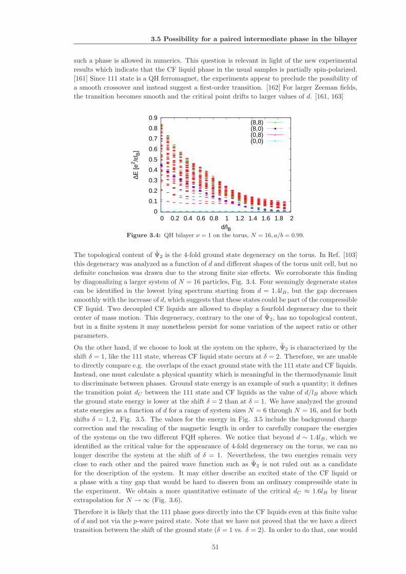
3.5 Possibility for a paired intermediate phase in the bilayer
such a phase is allowed in numerics. This question is relevant in light of the new experimental
results which indicate that the CF liquid phase in the usual samples is partially spin-polarized.
[161] Since 111 state is a QH ferromagnet, the experiments appear to preclude the possibility of
a smooth crossover and instead suggest a first-order transition. [162] For larger Zeeman fields,
the transition becomes smooth and the critical point drifts to larger values of d. [161, 163]
0
0.1
0.2
0.3
0.4
0.5
0.6
0.7
0.8
0.9
0 0.2 0.4 0.6 0.8 1 1.2 1.4 1.6 1.8 2
∆E [e
2 /εl B
]
d/lB
(8,8)(8,0)(0,8)(0,0)
Figure 3.4: QH bilayer ν = 1 on the torus, N = 16, a/b = 0.99.
The topological content of Ψ2 is the 4-fold ground state degeneracy on the torus. In Ref. [103]
this degeneracy was analyzed as a function of d and different shapes of the torus unit cell, but no
definite conclusion was drawn due to the strong finite size effects. We corroborate this finding
by diagonalizing a larger system of N = 16 particles, Fig. 3.4. Four seemingly degenerate states
can be identified in the lowest lying spectrum starting from d = 1.4lB , but the gap decreases
smoothly with the increase of d, which suggests that these states could be part of the compressible
CF liquid. Two decoupled CF liquids are allowed to display a fourfold degeneracy due to their
center of mass motion. This degeneracy, contrary to the one of Ψ2, has no topological content,
but in a finite system it may nonetheless persist for some variation of the aspect ratio or other
parameters.
On the other hand, if we choose to look at the system on the sphere, Ψ2 is characterized by the
shift δ = 1, like the 111 state, whereas CF liquid state occurs at δ = 2. Therefore, we are unable
to directly compare e.g. the overlaps of the exact ground state with the 111 state and CF liquids.
Instead, one must calculate a physical quantity which is meaningful in the thermodynamic limit
to discriminate between phases. Ground state energy is an example of such a quantity; it defines
the transition point dC between the 111 state and CF liquids as the value of d/lB above which
the ground state energy is lower at the shift δ = 2 than at δ = 1. We have analyzed the ground
state energies as a function of d for a range of system sizes N = 6 through N = 16, and for both
shifts δ = 1, 2, Fig. 3.5. The values for the energy in Fig. 3.5 include the background charge
correction and the rescaling of the magnetic length in order to carefully compare the energies
of the systems on the two different FQH spheres. We notice that beyond d ∼ 1.4lB , which we
identified as the critical value for the appearance of 4-fold degeneracy on the torus, we can no
longer describe the system at the shift of δ = 1. Nevertheless, the two energies remain very
close to each other and the paired wave function such as Ψ2 is not ruled out as a candidate
for the description of the system. It may either describe an excited state of the CF liquid or
a phase with a tiny gap that would be hard to discern from an ordinary compressible state in
the experiment. We obtain a more quantitative estimate of the critical dC ≈ 1.6lB by linear
extrapolation for N →∞ (Fig. 3.6).
Therefore it is likely that the 111 phase goes directly into the CF liquids even at this finite value
of d and not via the p-wave paired state. Note that we have not proved that the we have a direct
transition between the shift of the ground state (δ = 1 vs. δ = 2). In order to do that, one would
51
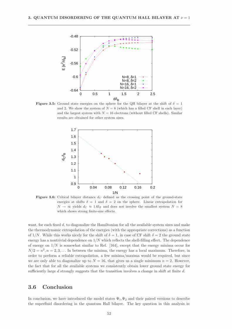
3. QUANTUM DISORDERING OF THE QUANTUM HALL BILAYER AT ν = 1
-0.64
-0.6
-0.56
-0.52
-0.48
0 0.5 1 1.5 2 2.5
E [e
2 /εl B
]
d/lB
N=8, δ=1N=8, δ=2
N=16, δ=1N=16, δ=2
Figure 3.5: Ground state energies on the sphere for the QH bilayer at the shift of δ = 1
and 2. We show the system of N = 8 (which has a filled CF shell in each layer)
and the largest system with N = 16 electrons (without filled CF shells). Similar
results are obtained for other system sizes.
0.9
1
1.1
1.2
1.3
1.4
1.5
1.6
1.7
0 0.04 0.08 0.12 0.16 0.2
d C/l B
1/NFigure 3.6: Critical bilayer distance dC defined as the crossing point of the ground-state
energies at shifts δ = 1 and δ = 2 on the sphere. Linear extrapolation for
N → ∞ yields dC ≈ 1.6lB and does not involve the smallest system N = 8
which shows strong finite-size effects.
want, for each fixed d, to diagonalize the Hamiltonian for all the available system sizes and make
the thermodynamic extrapolation of the energies (with the appropriate corrections) as a function
of 1/N . While this works nicely for the shift of δ = 1, in case of CF shift δ = 2 the ground state
energy has a nontrivial dependence on 1/N which reflects the shell-filling effect. The dependence
of energy on 1/N is somewhat similar to Ref. [164], except that the energy minima occur for
N/2 = n2, n = 2, 3, . . . In between the minima, the energy has a local maximum. Therefore, in
order to perform a reliable extrapolation, a few minima/maxima would be required, but since
we are only able to diagonalize up to N = 16, that gives us a single minimum n = 2. However,
the fact that for all the available systems we consistently obtain lower ground state energy for
sufficiently large d strongly suggests that the transition involves a change in shift at finite d.
3.6 Conclusion
In conclusion, we have introduced the model states Ψ1,Ψ2 and their paired versions to describe
the superfluid disordering in the quantum Hall bilayer. The key question in this analysis is:
52
3.6 Conclusion
what is the nature of the compressible phase at larger d/lB that still harbors some of the
intercorrelation present at smaller d/lB [96]?
The answer to this question cannot be given by looking at simple transport properties as both
Ψ1 and Ψ2 (in certain regimes) recover the semicircle law. [96] On the other hand, our picture
is certainly incomplete because it does not explicitly include the effects of disorder (which must
be very relevant for the physics of bilayer in the regimes d ∼ lB - a simple way to see this is
to look at the behavior of measured counterflow resistances [94, 95] ρCFxx , ρCF
xy that enter the
insulating regime very quickly after passing through ν = 1). Fertig and Murthy [97] provided a
realistic model for the effects of disorder and in their disorder-induced coherence network in the
incompressible phase of the bilayer, merons (vortices) are able to sweep by hopping across the
system, causing the activated behavior of resistance (dissipation) in counterflow. This finding is
consistent with our scenario based on the first family of wave functions (without weak pairing).
[105]
Quantum Hall bilayer was also probed using resonant Rayleigh scattering [165] for samples with
different tunneling amplitudes and when the in-plane magnetic field is present. They detected
a nonuniform spatial structure in the vicinity of the transition, suggesting a phase-separated
version of the ground state. If we think in terms of the phase-separated description, our picture
must be in the spirit of the Stern and Halperin proposal [149] but instead of the 1/2 compressible
phase coexisting in a phase separated picture with the superfluid phase (Ψ1), we assume the
existence of Ψ2.
On the other hand, in a translatory invariant system, the analysis on the basis of mixed states
does not preclude an intercorrelated, paired liquid state for the neutral sector. Numerical studies
give some evidence for a paired phase (Sec. 3.5.3) which is likely to be masked by the Fermi
liquid state appearing at a finite critical d.
53
3. QUANTUM DISORDERING OF THE QUANTUM HALL BILAYER AT ν = 1
54
Chapter 4
Transitions between
two-component and non-Abelian
states in bilayers with tunneling
In this Chapter we explore the possibility of creating non-Abelian states out of two-component
ones in the quantum Hall bilayer via tunneling mechanism. In particular we focus on the two
problems: (a) whether it is possible to create the Moore-Read Pfaffian in the LLL by appplying
tunneling to the two-component 331 state at ν = 1/2 in the LLL, and (b) we analyze the
transition from the 332 Halperin state to the Jain ν = 2/5 polarized state and examine whether
critical states, presumably gapless, such as Gaffnian or the permanent state, may play a role in
the transition region. Note that we neglect the electron spin in the present discussion. These
two problems represent two classes of transitions: in the first case, as we will show later, we
have an incompressible-compressible transition, whereas in the second case we have a transition
between the two incompressible states. Tunneling as a perturbation that drives the transition
from the two-component to a one-component FQH system was studied previously by analytical
[166] and numerical [167] means. Current Chapter summarizes the results of Refs. [121] and
[168].
4.1 Transition between 331 Halperin state and the Moore-
Read Pfaffian
As we saw in Sec. 1.5.2, owing to a mathematical identity, antisymmetrizing the neutral (Cauchy
determinant) part of Ψ331 between ↑ and ↓ leads to the Moore-Read Pfaffian. [117, 169] However,
such a procedure is a complex mathematical entity because it creates a state with different phys-
ical properties (non-Abelian statistics out of the Abelian), while we are interested in a physical
mechanism that mimics the antisymmetrization in an experimental situation. We restrict our
discussion to the Coulomb bilayer system, as a generic two-component system with the antisym-
metrization mechanism provided by the tunneling term ∼ −∆SASSx. The tunneling term favors
the even superposition (channel) where one expects to find a weakly paired (Moore-Read) phase.
We establish that this route towards the Moore-Read state is complicated by the presence of the
compressible CFL, which is the resulting phase for large tunneling. The results obtained within
the present bilayer model are relevant also in the study of wide quantum wells [118, 119, 120] as
the latter can, with moderate approximations, effectively be described by a bilayer Hamiltonian,
where the tunneling term mimics the effective confinement gap between the lowest and the first
excited electronic sublevel (see Chapter 5). [140] The remainder of this Section is organized as
55
4. TRANSITIONS BETWEEN TWO-COMPONENT AND NON-ABELIAN
STATES IN BILAYERS WITH TUNNELING
follows. We first introduce the BCS model due to Read and Green; this is an effective theory
which hides many subtleties of the physical system inside a few parameters such as the single
particle dispersion or the pairing function. These parameters will likely be modified with the
change in tunneling, but we will, nevertheless, verify that despite its crudeness, BCS predictions
are in agreement with exact diagonalization calculations, so that combining the two approaches
we can obtain a complete picture of the transition. At the end, we will discuss an extension of
the BCS model in a way that surpasses the exact diagonalization capabilities, but which can
give us a clue as to how one can engineer the Pfaffian state in bilayers exclusively in the LLL.
4.1.1 BCS model for half-filled Landau level
At ν = 1/2 (or ν = 2 + 1/2), the CFs experience a zero net magnetic field, [53, 170] and if we
limit ourselves to the neutral part of |ΨPf〉 (1.38), they may be described within the framework
of the effective BCS model introduced in the seminal work of Read and Green. [171] We consider
the system to be at zero temperature and neglect fluctuations in the Chern-Simons gauge field
that are related to the charge part of |ΨPf〉. [172] The Hamiltonian which describes the Cauchy
pairing between ↑ and ↓ particles with tunneling ∆SAS reads
H =∑
k
[
ǫk(c†k↑ck↑ + c†k↓ck↓) +(
∆kc†k↑c
†−k↓ + H.c.
)
− ∆SAS
2(c†k↑ck↓ + c†k↓ck↑)
]
, (4.1)
where ǫk = ǫk−µ, in terms of the putative CF dispersion relation ǫk and the chemical potential
µ, which is assumed positive µ > 0. Notice that because of the vanishing net magnetic field,
the 2D wave vector k = (kx, ky) is again a good quantum number. The order parameter ∆k =
∆0(kx − iky) is chosen to describe p-wave pairing and ∆0 is a constant. This may seem like
a drastic simplification, but it leads to the physical conclusions [171] which agree with exact
diagonalization results, as we show below. Furthermore, there is a number of assumptions
implicit to the effectivel model defined by (4.1), such as that ∆k and µ are not renormalized by
the tunneling (while they should be evaluated self-consistently from the Bogoliubov-de Gennes
equations) and that CFs have a single-particle-like dispersion relation with a well-defined mass.
For fixed tunneling, ∆k is also expected to depend on the interaction and the well width or bilayer
distance. Note also that as it stands, Hamiltonian (4.1) does not distinguish between Landau
levels i.e. it has the same form for the LLL and first excited LL and detailed microscopic theory
is needed to model ∆k and ǫk to account for their difference. All of these effects are outside the
scope of the treatment in this Chapter.
With the help of the even, ck,e = (ck,↑ + ck,↓)/√
2, and odd spin combinations ck,o = (ck,↑ −ck,↓)/
√2, the Hamiltonian (4.1) decouples into an even and odd channel, [171] H = He +Ho,
where (the index τ denotes the even and odd channel, τ = e, o)
Hτ =∑
k
[
(ǫk − µτ )c†k,τ ck,τ +(
∆τkc
†k,τ c
†−k,τ + H.c.
)]
, (4.2)
in terms of the chemical potentials µe = µ+∆SAS/2 and µo = µ−∆SAS/2 for the even and odd
channels, respectively. Furthermore, the even/odd p-wave order parameters read ∆ek = ∆k/2 =
(∆0/2)(kx − iky) and ∆ok = ∆−k/2 = −(∆0/2)(kx − iky).
For moderate tunnelings, it is instructive to view the effective chemical potential µeff of the
whole system as the weighted sum of the two channels, µeff = Pµe + (1 − P )µo. In this crude
approximation P measures the population of the even channel (1/2 ≤ P ≤ 1) and may have
a complicated dependence on ∆SAS . In particular, for some values of ∆SAS we may be below
the critical line µeff = P∆SAS defined by µo = 0 and inside the non-Abelian (Pfaffian) phase.
However, in the limit of large tunneling, the system is dominated by the even channel and
the chemical potential of the whole system is µeff = µe because P = 1. Remember that the
associated BCS wave function in the even channel reads
|ψBCS〉 =∏
k
(
1 + gkc†k,ec
†−k,e
)
|vacuum〉, (4.3)
56
4.1 Transition between 331 Halperin state and the Moore-Read Pfaffian
in terms of the pairing function gk = vk/uk = −(Ek,e − ǫk,e)/∆e∗k ∼ µe/∆0 (see below). One
notices then that an increase of the chemical potential µeff controlled by the large value of the
tunneling parameter ∆SAS is equivalent to a reduction of the order parameter ∆0. Therefore
the BCS system will eventually be transformed into the one of the Fermi liquid. We can see this
more explicitly by examining the relevant excitations of the even channel, [171]
E =√
(ǫk − µe)2 + ∆20k
2, (4.4)
in the limit of large µe around k = |k| = 0. They become unstable and k = 0 becomes a
point of local maximum. The minimum is expected to move to |k| = kF , the Fermi momentum.
[171] Therefore if ∆0 does not “renormalize” with increasing ∆SAS , the net effect of the strong
tunneling (µe ≫ µ) on the Cauchy pairing is to drive the system into a Fermi liquid. This is
not unexpected because one retrieves an effective one-component system in this limit, where all
particles are “polarized“ in the even channel. However, even if the system becomes compressible
in order to find a minimum at |k| = kF , the wave function (4.3) still describes its excited state.
Therefore, Pfaffian in this system may arise either as an excited state of the CFL or as an
intermediate state before complete polarization. We revisit the BCS approach in Sec. 4.1.4,
with a slightly different perspective in which the antisymmetrization is imposed, in a functional
formalism, with the help of a Lagrangian multiplier which plays a similar role as the present
tunneling term ∆SAS .
As we pointed out earlier, the population of the even channel P may be a complicated function
of tunneling. In the following section we use exact diagonalization of small finite systems in
order to get a hint of the form of this dependence P = P (∆SAS) and determine the nature of
possible phases as P increases from 1/2 to 1.
4.1.2 Exact diagonalization
Here we study the full interacting quantum Hall bilayer Hamiltonian for small finite systems in
the presence of tunneling, [110, 173]
H = −∆SASSx +∑
i<j,σ∈↑,↓V intra(riσ − rjσ) +
∑
i,j
V inter(ri↑ − rj↓), (4.5)
where in coordinate representation we have 2Sx =∫
dr[
Ψ†↑(r)Ψ↓(r) + H.c.
]
, Ψ†σ(r) creates a
particle at the position r in the layer σ. We have decomposed the interaction into terms between
electrons belonging to the same layer (V intra) and those residing in opposite layers (V inter). We
consider a short-range interaction, defined as
V intra331 (r) = V1∇2δ(r), V inter
331 (r) = V0δ(r), (4.6)
which produces the 331 state as the densest and unique zero energy state when V0, V1 are chosen
positive. [42, 65] We also consider long-range Coulomb interaction,
V intraCoul (r) = e2/ǫr, V inter
Coul (r) = e2/ǫ√
r2 + d2, (4.7)
where d is the distance between layers. Note that we are diagonalizing an explicitly lowest
Landau level problem. We fix the total number of particles in our calculations to be an even
integer and, unless stated otherwise, take d = lB , which merely sets the range for the distance
between the layers where the Coulomb ground state is supposed to be fairly well described by the
331 wave function (compare with Sec. 2.2.2). In what follows, we consider spherical and torus
geometry for exact diagonalization. When we compare the exact ground state with |ΨPf〉, it is
understood that the latter is defined in the even basis i.e. single-particle states are understood
to be even combinations of the original ↑, ↓ states.
In Fig. 4.1 we present results of exact diagonalization on the sphere for the short-range (331)
Hamiltonian (4.6) and long-range (Coulomb) Hamiltonian (4.7). 331 and Pfaffian trial states
57
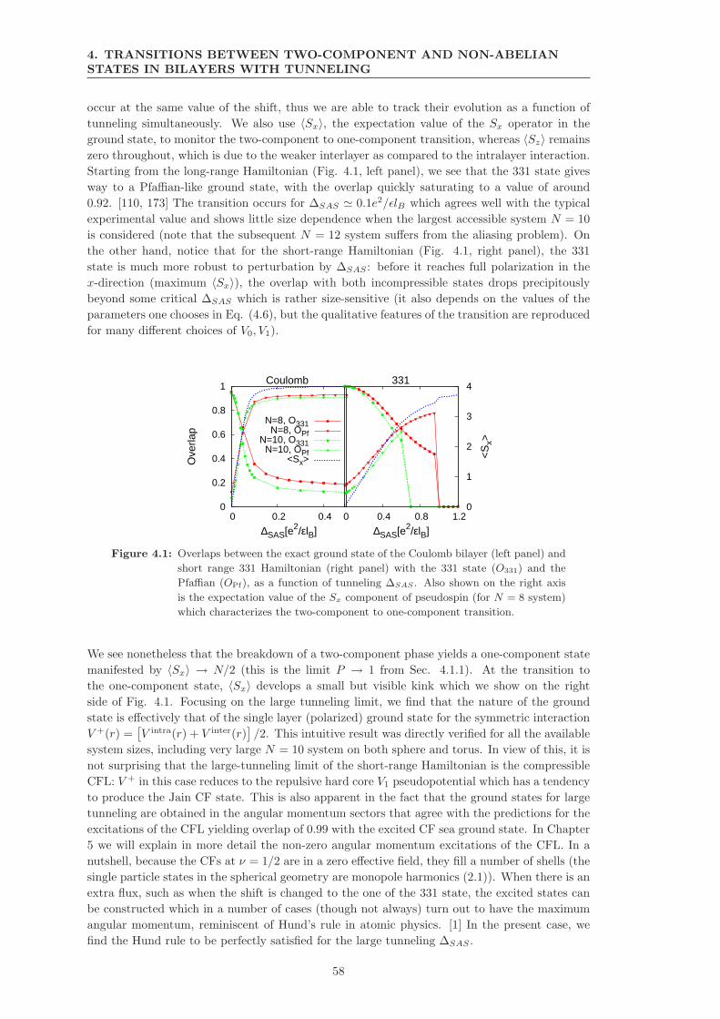
4. TRANSITIONS BETWEEN TWO-COMPONENT AND NON-ABELIAN
STATES IN BILAYERS WITH TUNNELING
occur at the same value of the shift, thus we are able to track their evolution as a function of
tunneling simultaneously. We also use 〈Sx〉, the expectation value of the Sx operator in the
ground state, to monitor the two-component to one-component transition, whereas 〈Sz〉 remains
zero throughout, which is due to the weaker interlayer as compared to the intralayer interaction.
Starting from the long-range Hamiltonian (Fig. 4.1, left panel), we see that the 331 state gives
way to a Pfaffian-like ground state, with the overlap quickly saturating to a value of around
0.92. [110, 173] The transition occurs for ∆SAS ≃ 0.1e2/ǫlB which agrees well with the typical
experimental value and shows little size dependence when the largest accessible system N = 10
is considered (note that the subsequent N = 12 system suffers from the aliasing problem). On
the other hand, notice that for the short-range Hamiltonian (Fig. 4.1, right panel), the 331
state is much more robust to perturbation by ∆SAS : before it reaches full polarization in the
x-direction (maximum 〈Sx〉), the overlap with both incompressible states drops precipitously
beyond some critical ∆SAS which is rather size-sensitive (it also depends on the values of the
parameters one chooses in Eq. (4.6), but the qualitative features of the transition are reproduced
for many different choices of V0, V1).
0
0.2
0.4
0.6
0.8
1
0 0.2 0.4
Ove
rlap
∆SAS[e2/εlB]
Coulomb
N=8, O331N=8, OPf
N=10, O331N=10, OPf
<Sx>
0 0.4 0.8 1.2 0
1
2
3
4
<S
x>
∆SAS[e2/εlB]
331
Figure 4.1: Overlaps between the exact ground state of the Coulomb bilayer (left panel) and
short range 331 Hamiltonian (right panel) with the 331 state (O331) and the
Pfaffian (OPf), as a function of tunneling ∆SAS . Also shown on the right axis
is the expectation value of the Sx component of pseudospin (for N = 8 system)
which characterizes the two-component to one-component transition.
We see nonetheless that the breakdown of a two-component phase yields a one-component state
manifested by 〈Sx〉 → N/2 (this is the limit P → 1 from Sec. 4.1.1). At the transition to
the one-component state, 〈Sx〉 develops a small but visible kink which we show on the right
side of Fig. 4.1. Focusing on the large tunneling limit, we find that the nature of the ground
state is effectively that of the single layer (polarized) ground state for the symmetric interaction
V +(r) =[
V intra(r) + V inter(r)]
/2. This intuitive result was directly verified for all the available
system sizes, including very large N = 10 system on both sphere and torus. In view of this, it is
not surprising that the large-tunneling limit of the short-range Hamiltonian is the compressible
CFL: V + in this case reduces to the repulsive hard core V1 pseudopotential which has a tendency
to produce the Jain CF state. This is also apparent in the fact that the ground states for large
tunneling are obtained in the angular momentum sectors that agree with the predictions for the
excitations of the CFL yielding overlap of 0.99 with the excited CF sea ground state. In Chapter
5 we will explain in more detail the non-zero angular momentum excitations of the CFL. In a
nutshell, because the CFs at ν = 1/2 are in a zero effective field, they fill a number of shells (the
single particle states in the spherical geometry are monopole harmonics (2.1)). When there is an
extra flux, such as when the shift is changed to the one of the 331 state, the excited states can
be constructed which in a number of cases (though not always) turn out to have the maximum
angular momentum, reminiscent of Hund’s rule in atomic physics. [1] In the present case, we
find the Hund rule to be perfectly satisfied for the large tunneling ∆SAS .
58
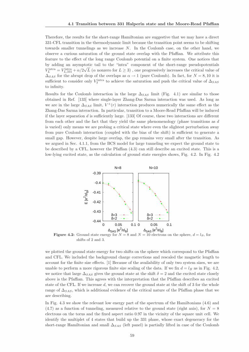
4.1 Transition between 331 Halperin state and the Moore-Read Pfaffian
Therefore, the results for the short-range Hamiltonian are suggestive that we may have a direct
331-CFL transition in the thermodynamic limit because the transition point seems to be shifting
towards smaller tunnelings as we increase N . In the Coulomb case, on the other hand, we
observe a curious saturation of the ground state overlap with the Pfaffian. We attribute this
feature to the effect of the long range Coulomb potential on a finite system. One notices that
by adding an asymptotic tail to the “intra” component of the short-range pseudopotentials
V intraL = V intra
L,331 +α/2√L (α nonzero for L ≥ 3) , one progressively increases the critical value of
∆SAS for the abrupt drop of the overlaps as α→ 1 (pure Coulomb). In fact, for N = 8, 10 it is
sufficient to consider only V intra3 to achieve the saturation and push the critical value of ∆SAS
to infinity.
Results for the Coulomb interaction in the large ∆SAS limit (Fig. 4.1) are similar to those
obtained in Ref. [133] where single-layer Zhang-Das Sarma interaction was used. As long as
we are in the large ∆SAS limit, V +(r) interaction produces numerically the same effect as the
Zhang-Das Sarma interaction. In particular, transition to a Moore-Read Pfaffian will be induced
if the layer separation d is sufficiently large. [133] Of course, these two interactions are different
from each other and the fact that they yield the same phenomenology (phase transitions as d
is varied) only means we are probing a critical state where even the slightest perturbation away
from pure Coulomb interaction (coupled with the bias of the shift) is sufficient to generate a
small gap. However, despite large overlap, the gap remains very small after the transition. As
we argued in Sec. 4.1.1, from the BCS model for large tunneling we expect the ground state to
be described by a CFL, however the Pfaffian (4.3) can still describe an excited state. This is a
low-lying excited state, as the calculation of ground state energies shows, Fig. 4.2. In Fig. 4.2
-0.44
-0.43
-0.42
-0.41
-0.4
-0.39
0 0.05 0.1
E [e
2 /εl B
]
∆SAS [e2/εlB]
N=8
δ=3δ=2
0 0.05 0.1
∆SAS [e2/εlB]
N=10
δ=3δ=2
Figure 4.2: Ground state energy for N = 8 and N = 10 electrons on the sphere, d = lB , for
shifts of 2 and 3.
we plotted the ground state energy for two shifts on the sphere which correspond to the Pfaffian
and CFL. We included the background charge corrections and rescaled the magnetic length to
account for the finite size effects. [1] Because of the availability of only two system sizes, we are
unable to perform a more rigorous finite size scaling of the data. If we fix d = lB as in Fig. 4.2,
we notice that large ∆SAS gives the ground state at the shift δ = 2 and the excited state closely
above is the Pfaffian. This agrees with the interpretation that the Pfaffian describes an excited
state of the CFL. If we increase d, we can recover the ground state at the shift of 3 for the whole
range of ∆SAS , which is additional evidence of the critical nature of the Pfaffian phase that we
are describing.
In Fig. 4.3 we show the relevant low energy part of the spectrum of the Hamiltonians (4.6) and
(4.7) as a function of tunneling, measured relative to the ground state (right axis), for N = 8
electrons on the torus and the fixed aspect ratio 0.97 in the vicinity of the square unit cell. We
identify the multiplet of 4 states that build up the 331 phase, whose exact degeneracy for the
short-range Hamiltonian and small ∆SAS (left panel) is partially lifted in case of the Coulomb
59
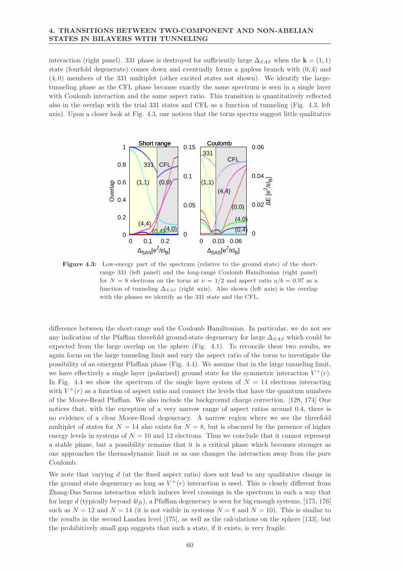
4. TRANSITIONS BETWEEN TWO-COMPONENT AND NON-ABELIAN
STATES IN BILAYERS WITH TUNNELING
interaction (right panel). 331 phase is destroyed for sufficiently large ∆SAS when the k = (1, 1)
state (fourfold degenerate) comes down and eventually forms a gapless branch with (0, 4) and
(4, 0) members of the 331 multiplet (other excited states not shown). We identify the large-
tunneling phase as the CFL phase because exactly the same spectrum is seen in a single layer
with Coulomb interaction and the same aspect ratio. This transition is quantitatively reflected
also in the overlap with the trial 331 states and CFL as a function of tunneling (Fig. 4.3, left
axis). Upon a closer look at Fig. 4.3, one notices that the torus spectra suggest little qualitative
0
0.2
0.4
0.6
0.8
1
0 0.1 0.2 0
0.05
0.1
0.15
Ove
rlap
∆SAS[e2/εlB]
331 CFL
(1,1) (0,0)
(4,4)(0,4)(4,0)
Short range Coulomb
0 0.03 0.06 0
0.02
0.04
0.06
∆E [e
2 /εl B
]
∆SAS[e2/εlB]
331CFL
(1,1)
(0,0)
(4,4)
(0,4)
(4,0)
Short range Coulomb
Figure 4.3: Low-energy part of the spectrum (relative to the ground state) of the short-
range 331 (left panel) and the long-range Coulomb Hamiltonian (right panel)
for N = 8 electrons on the torus at ν = 1/2 and aspect ratio a/b = 0.97 as a
function of tunneling ∆SAS (right axis). Also shown (left axis) is the overlap
with the phases we identify as the 331 state and the CFL.
difference between the short-range and the Coulomb Hamiltonian. In particular, we do not see
any indication of the Pfaffian threefold ground-state degeneracy for large ∆SAS which could be
expected from the large overlap on the sphere (Fig. 4.1). To reconcile these two results, we
again focus on the large tunneling limit and vary the aspect ratio of the torus to investigate the
possibility of an emergent Pfaffian phase (Fig. 4.4). We assume that in the large tunneling limit,
we have effectively a single layer (polarized) ground state for the symmetric interaction V +(r).
In Fig. 4.4 we show the spectrum of the single layer system of N = 14 electrons interacting
with V +(r) as a function of aspect ratio and connect the levels that have the quantum numbers
of the Moore-Read Pfaffian. We also include the background charge correction. [128, 174] One
notices that, with the exception of a very narrow range of aspect ratios around 0.4, there is
no evidence of a clear Moore-Read degeneracy. A narrow region where we see the threefold
multiplet of states for N = 14 also exists for N = 8, but is obscured by the presence of higher
energy levels in systems of N = 10 and 12 electrons. Thus we conclude that it cannot represent
a stable phase, but a possibility remains that it is a critical phase which becomes stronger as
one approaches the thermodynamic limit or as one changes the interaction away from the pure
Coulomb.
We note that varying d (at the fixed aspect ratio) does not lead to any qualitative change in
the ground state degeneracy as long as V +(r) interaction is used. This is clearly different from
Zhang-Das Sarma interaction which induces level crossings in the spectrum in such a way that
for large d (typically beyond 4lB), a Pfaffian degeneracy is seen for big enough systems, [175, 176]
such as N = 12 and N = 14 (it is not visible in systems N = 8 and N = 10). This is similar to
the results in the second Landau level [175], as well as the calculations on the sphere [133], but
the prohibitively small gap suggests that such a state, if it exists, is very fragile.
60
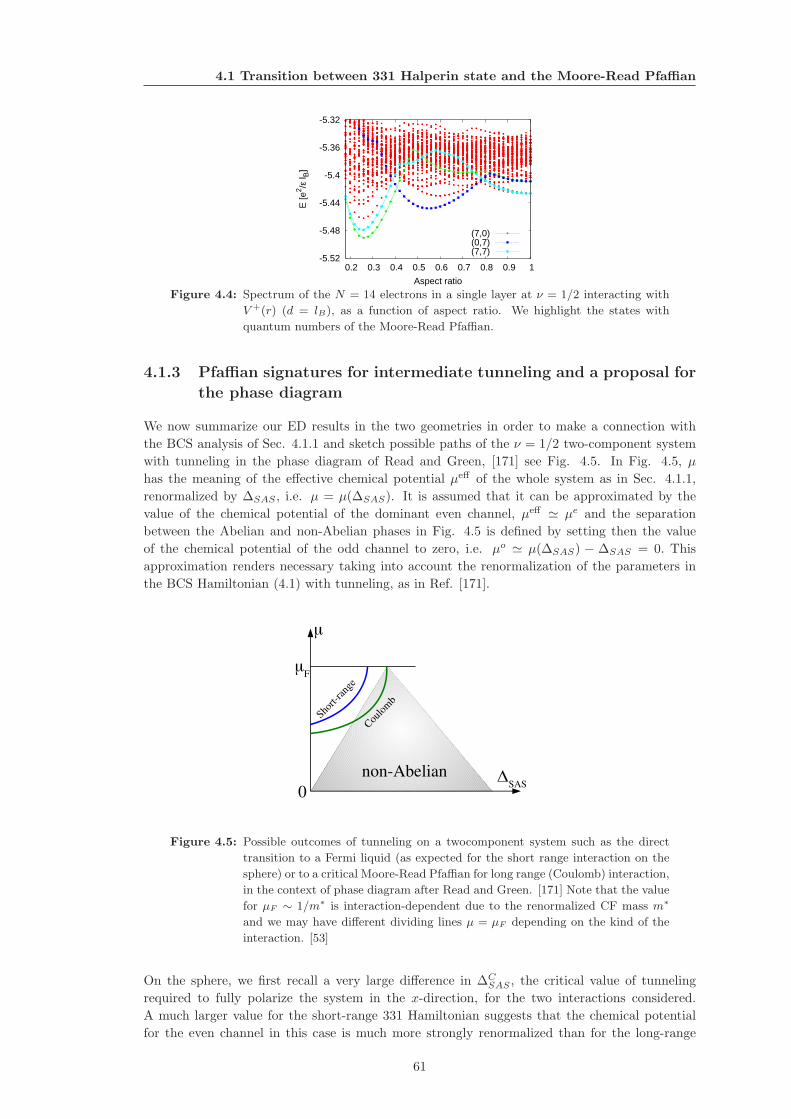
4.1 Transition between 331 Halperin state and the Moore-Read Pfaffian
-5.52
-5.48
-5.44
-5.4
-5.36
-5.32
0.2 0.3 0.4 0.5 0.6 0.7 0.8 0.9 1
E [e
2 /ε l B
]
Aspect ratio
(7,0)(0,7)(7,7)
Figure 4.4: Spectrum of the N = 14 electrons in a single layer at ν = 1/2 interacting with
V +(r) (d = lB), as a function of aspect ratio. We highlight the states with
quantum numbers of the Moore-Read Pfaffian.
4.1.3 Pfaffian signatures for intermediate tunneling and a proposal for
the phase diagram
We now summarize our ED results in the two geometries in order to make a connection with
the BCS analysis of Sec. 4.1.1 and sketch possible paths of the ν = 1/2 two-component system
with tunneling in the phase diagram of Read and Green, [171] see Fig. 4.5. In Fig. 4.5, µ
has the meaning of the effective chemical potential µeff of the whole system as in Sec. 4.1.1,
renormalized by ∆SAS , i.e. µ = µ(∆SAS). It is assumed that it can be approximated by the
value of the chemical potential of the dominant even channel, µeff ≃ µe and the separation
between the Abelian and non-Abelian phases in Fig. 4.5 is defined by setting then the value
of the chemical potential of the odd channel to zero, i.e. µo ≃ µ(∆SAS) − ∆SAS = 0. This
approximation renders necessary taking into account the renormalization of the parameters in
the BCS Hamiltonian (4.1) with tunneling, as in Ref. [171].
Figure 4.5: Possible outcomes of tunneling on a twocomponent system such as the direct
transition to a Fermi liquid (as expected for the short range interaction on the
sphere) or to a critical Moore-Read Pfaffian for long range (Coulomb) interaction,
in the context of phase diagram after Read and Green. [171] Note that the value
for µF ∼ 1/m∗ is interaction-dependent due to the renormalized CF mass m∗
and we may have different dividing lines µ = µF depending on the kind of the
interaction. [53]
On the sphere, we first recall a very large difference in ∆CSAS , the critical value of tunneling
required to fully polarize the system in the x-direction, for the two interactions considered.
A much larger value for the short-range 331 Hamiltonian suggests that the chemical potential
for the even channel in this case is much more strongly renormalized than for the long-range
61
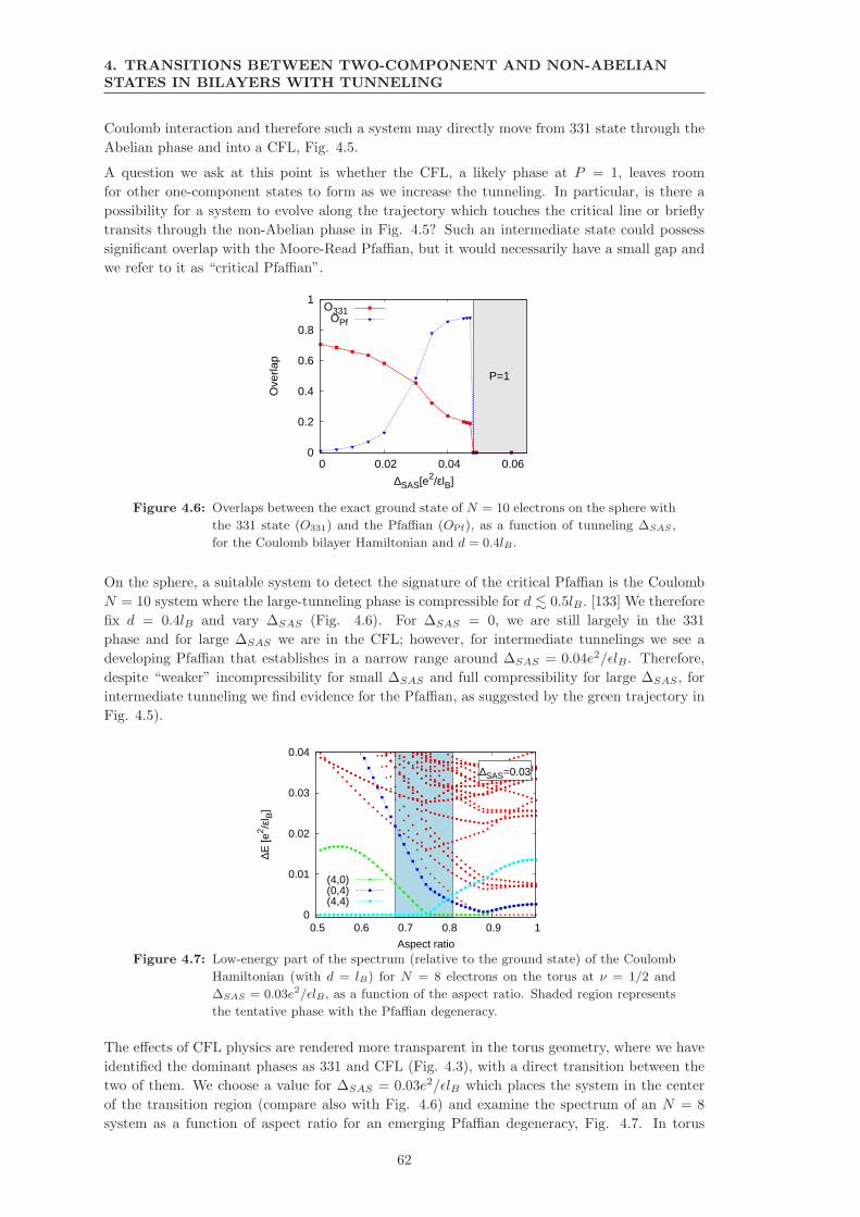
4. TRANSITIONS BETWEEN TWO-COMPONENT AND NON-ABELIAN
STATES IN BILAYERS WITH TUNNELING
Coulomb interaction and therefore such a system may directly move from 331 state through the
Abelian phase and into a CFL, Fig. 4.5.
A question we ask at this point is whether the CFL, a likely phase at P = 1, leaves room
for other one-component states to form as we increase the tunneling. In particular, is there a
possibility for a system to evolve along the trajectory which touches the critical line or briefly
transits through the non-Abelian phase in Fig. 4.5? Such an intermediate state could possess
significant overlap with the Moore-Read Pfaffian, but it would necessarily have a small gap and
we refer to it as “critical Pfaffian”.
0
0.2
0.4
0.6
0.8
1
0 0.02 0.04 0.06
Ove
rlap
∆SAS[e2/εlB]
P=1
O331OPf
Figure 4.6: Overlaps between the exact ground state of N = 10 electrons on the sphere with
the 331 state (O331) and the Pfaffian (OPf), as a function of tunneling ∆SAS ,
for the Coulomb bilayer Hamiltonian and d = 0.4lB .
On the sphere, a suitable system to detect the signature of the critical Pfaffian is the Coulomb
N = 10 system where the large-tunneling phase is compressible for d . 0.5lB . [133] We therefore
fix d = 0.4lB and vary ∆SAS (Fig. 4.6). For ∆SAS = 0, we are still largely in the 331
phase and for large ∆SAS we are in the CFL; however, for intermediate tunnelings we see a
developing Pfaffian that establishes in a narrow range around ∆SAS = 0.04e2/ǫlB . Therefore,
despite “weaker” incompressibility for small ∆SAS and full compressibility for large ∆SAS , for
intermediate tunneling we find evidence for the Pfaffian, as suggested by the green trajectory in
Fig. 4.5).
0
0.01
0.02
0.03
0.04
0.5 0.6 0.7 0.8 0.9 1
∆E [e
2 /εl B
]
Aspect ratio
(4,0)(0,4)(4,4)
∆SAS=0.03
Figure 4.7: Low-energy part of the spectrum (relative to the ground state) of the Coulomb
Hamiltonian (with d = lB) for N = 8 electrons on the torus at ν = 1/2 and
∆SAS = 0.03e2/ǫlB , as a function of the aspect ratio. Shaded region represents
the tentative phase with the Pfaffian degeneracy.
The effects of CFL physics are rendered more transparent in the torus geometry, where we have
identified the dominant phases as 331 and CFL (Fig. 4.3), with a direct transition between the
two of them. We choose a value for ∆SAS = 0.03e2/ǫlB which places the system in the center
of the transition region (compare also with Fig. 4.6) and examine the spectrum of an N = 8
system as a function of aspect ratio for an emerging Pfaffian degeneracy, Fig. 4.7. In torus
62
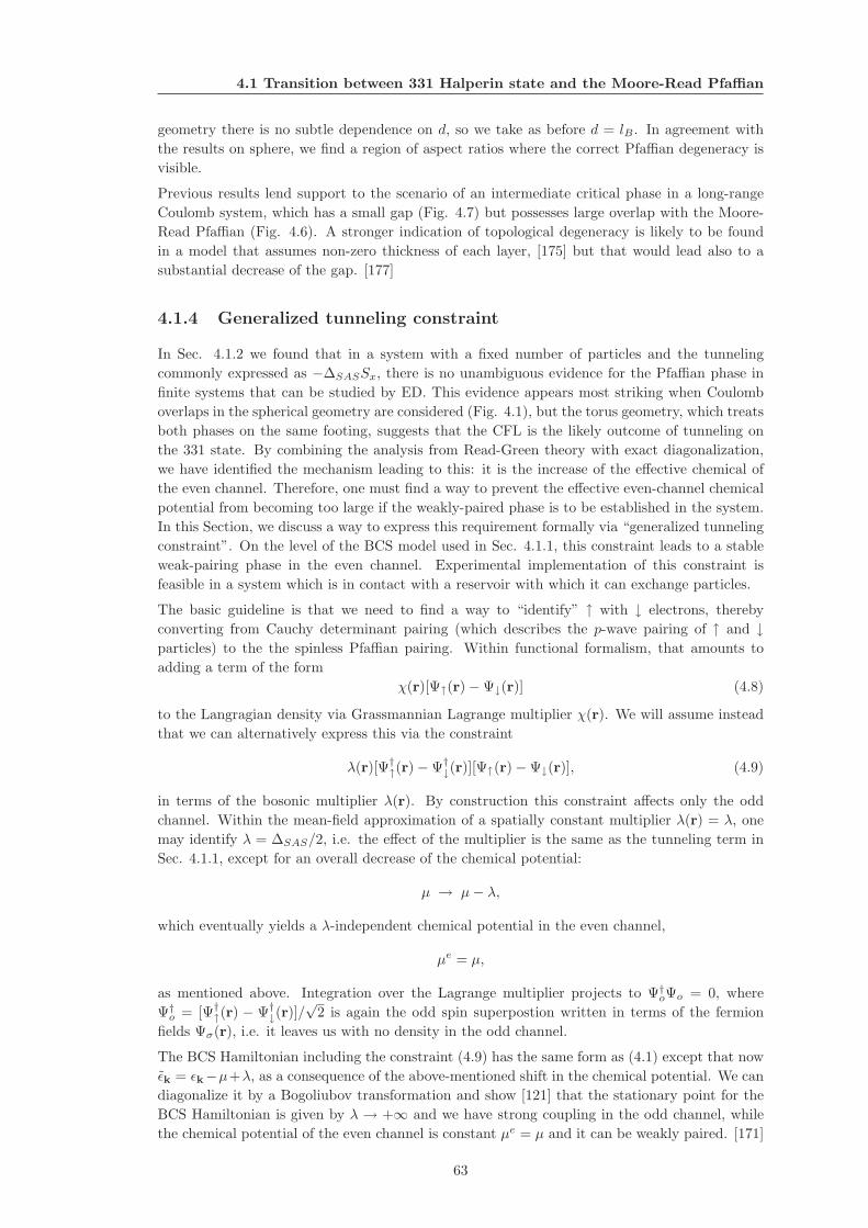
4.1 Transition between 331 Halperin state and the Moore-Read Pfaffian
geometry there is no subtle dependence on d, so we take as before d = lB . In agreement with
the results on sphere, we find a region of aspect ratios where the correct Pfaffian degeneracy is
visible.
Previous results lend support to the scenario of an intermediate critical phase in a long-range
Coulomb system, which has a small gap (Fig. 4.7) but possesses large overlap with the Moore-
Read Pfaffian (Fig. 4.6). A stronger indication of topological degeneracy is likely to be found
in a model that assumes non-zero thickness of each layer, [175] but that would lead also to a
substantial decrease of the gap. [177]
4.1.4 Generalized tunneling constraint
In Sec. 4.1.2 we found that in a system with a fixed number of particles and the tunneling
commonly expressed as −∆SASSx, there is no unambiguous evidence for the Pfaffian phase in
finite systems that can be studied by ED. This evidence appears most striking when Coulomb
overlaps in the spherical geometry are considered (Fig. 4.1), but the torus geometry, which treats
both phases on the same footing, suggests that the CFL is the likely outcome of tunneling on
the 331 state. By combining the analysis from Read-Green theory with exact diagonalization,
we have identified the mechanism leading to this: it is the increase of the effective chemical of
the even channel. Therefore, one must find a way to prevent the effective even-channel chemical
potential from becoming too large if the weakly-paired phase is to be established in the system.
In this Section, we discuss a way to express this requirement formally via “generalized tunneling
constraint”. On the level of the BCS model used in Sec. 4.1.1, this constraint leads to a stable
weak-pairing phase in the even channel. Experimental implementation of this constraint is
feasible in a system which is in contact with a reservoir with which it can exchange particles.
The basic guideline is that we need to find a way to “identify” ↑ with ↓ electrons, thereby
converting from Cauchy determinant pairing (which describes the p-wave pairing of ↑ and ↓particles) to the the spinless Pfaffian pairing. Within functional formalism, that amounts to
adding a term of the form
χ(r)[Ψ↑(r)−Ψ↓(r)] (4.8)
to the Langragian density via Grassmannian Lagrange multiplier χ(r). We will assume instead
that we can alternatively express this via the constraint
λ(r)[Ψ†↑(r)−Ψ†
↓(r)][Ψ↑(r)−Ψ↓(r)], (4.9)
in terms of the bosonic multiplier λ(r). By construction this constraint affects only the odd
channel. Within the mean-field approximation of a spatially constant multiplier λ(r) = λ, one
may identify λ = ∆SAS/2, i.e. the effect of the multiplier is the same as the tunneling term in
Sec. 4.1.1, except for an overall decrease of the chemical potential:
µ → µ− λ,
which eventually yields a λ-independent chemical potential in the even channel,
µe = µ,
as mentioned above. Integration over the Lagrange multiplier projects to Ψ†oΨo = 0, where
Ψ†o = [Ψ†
↑(r) − Ψ†↓(r)]/
√2 is again the odd spin superpostion written in terms of the fermion
fields Ψσ(r), i.e. it leaves us with no density in the odd channel.
The BCS Hamiltonian including the constraint (4.9) has the same form as (4.1) except that now
ǫk = ǫk−µ+λ, as a consequence of the above-mentioned shift in the chemical potential. We can
diagonalize it by a Bogoliubov transformation and show [121] that the stationary point for the
BCS Hamiltonian is given by λ → +∞ and we have strong coupling in the odd channel, while
the chemical potential of the even channel is constant µe = µ and it can be weakly paired. [171]
63
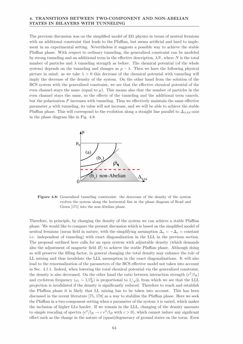
4. TRANSITIONS BETWEEN TWO-COMPONENT AND NON-ABELIAN
STATES IN BILAYERS WITH TUNNELING
The previous discussion was on the simplified model of 331 physics in terms of neutral fermions
with an additional constraint that leads to the Pfaffian, but seems artificial and hard to imple-
ment in an experimental setting. Nevertheless it suggests a possible way to achieve the stable
Pfaffian phase. With respect to ordinary tunneling, the generalized constraint can be modeled
by strong tunneling and an additional term in the effective description, λN , where N is the total
number of particles and λ tunneling strength as before. The chemical potential (of the whole
system) depends on the tunneling and changes as µ − λ. Then we have the following physical
picture in mind: as we take λ > 0 this decrease of the chemical potential with tunneling will
imply the decrease of the density of the system. On the other hand from the solution of the
BCS system with the generalized constraint, we see that the effective chemical potential of the
even channel stays the same (equal to µ). This means also that the number of particles in the
even channel stays the same, so the effects of the tunneling and the additional term cancels,
but the polarization P increases with tunneling. Thus we effectively maintain the same effective
parameter µ with tunneling, its value will not increase, and we will be able to achieve the stable
Pfaffian phase. This will correspond to the evolution along a straight line parallel to ∆SAS-axis
in the phase diagram like in Fig. 4.8.
Figure 4.8: Generalized tunneling contstraint: the descrease of the density of the system
evolves the system along the horizontal line in the phase diagram of Read and
Green [171] into the non-Abelian phase.
Therefore, in principle, by changing the density of the system we can achieve a stable Pfaffian
phase. We would like to compare the present discussion which is based on the simplified model of
neutral fermions (mean field in nature, with the simplifying assumption ∆o = −∆e = constant
i.e. independent of tunneling) with exact diagonalization in the LLL in the previous section.
The proposal outlined here calls for an open system with adjustable density (which demands
also the adjustment of magnetic field B) to achieve the stable Pfaffian phase. Although doing
so will preserve the filling factor, in general changing the total density may enhance the role of
LL mixing and thus invalidate the LLL assumption in the exact diagonalizations. It will also
lead to the renormalization of the parameters of the BCS effective model not taken into account
in Sec. 4.1.1. Indeed, when lowering the total chemical potential via the generalized constraint,
the density is also decreased. On the other hand the ratio between interaction strength (e2/lB)
and cyclotron frequency (ωc ∼ 1/l2B) is proportional to 1/√ρ, from which we see that the LLL
projection is invalidated if the density is significantly reduced. Therefore to reach and establish
the Pfaffian phase it is likely that LL mixing has to be taken into account. This has been
discussed in the recent literature [75, 178] as a way to stabilize the Pfaffian phase. Here we seek
the Pfaffian in a two-component setting when a parameter of the system λ is varied, which makes
the inclusion of higher LLs harder. If we remain in the LLL, changing of the density amounts
to simple rescaling of spectra (e2/lB → c e2/lB with c > 0), which cannot induce any signficant
effect such as the change in the nature of (quasi)degeneracy of ground states on the torus. Even
64
4.2 Transition from 332 Halperin to Jain’s state at ν = 2/5
if the evidence for a Pfaffian phase is rather weak for the system sizes studied here, one may
hope that the increase of these sizes will improve the case for such a state in the LLL as the odd
channel may assume the role of the first excited Landau level before a complete polarization.
4.2 Transition from 332 Halperin to Jain’s state at ν = 2/5
In this Section we study the transition from Halperin’s two-component 332 state (1.45) to the
one-component Jain state at the filling factor ν = 2/5 (1.36) via tunneling. The interest is
threefold: we would like to find out (a) about the nature of quantum phase transitions between
topological phases which are similar (332 and Jain’s state have the same ground state degeneracy
[129, 143, 179] but different shift [42, 180]), (b) we would like to find if Gaffnian [82] can be
characterized as a critical state in these circumstances when the gap closes, and (c) we explore
possible consequences for the effective description of the Jain state due to a better understanding
of the transition.
4.2.1 The system under consideration
We consider the bilayer system at the filling factor ν = 2/5 defined by the Hamiltonian (4.5).
As we outlined in Sec. 1.5.3, in the small tunneling regime the ground state of the Hamiltonian
(4.5) at ν = 2/5 is the 332 Halperin state for two distinguishable species of electrons. Due to
the fact that the correlation exponents between electrons of the same layer are bigger than those
between electrons of the opposite layers, we expect the 332 wave function (1.45) to be more
appropriate for non-zero d e.g. in the range d ∼ lB . However, as it possesses the necessary
symmetry properties, [42] it can be a candidate also for d = 0. The properties of the 332 wave
function (1.45) were numerically verified in Ref. [108].
As the tunneling strength ∆SAS is increased, the electrons find it energetically favorable to be
in the superposition of two layers, ↑ + ↓, and the system loses its two-component character.
The effective single-component state is characterized by full polarization in the x-direction. At
ν = 2/5 in the LLL, a compelling candidate for the polarized state is Jain’s CF state, (1.36).
Note that a single index now suffices to label the electron coordinates as the pseudospin index
is implicitly assumed to be ↑ + ↓. An alternative candidate for the polarized state at ν = 2/5
exists, which is the so-called Gaffnian state, (1.55). In the notation of Eq. (1.55) one can think
of the Gaffnian as originating from the two-component 332 state with the additional pairing
represented by the permanent. [117, 181] The two-component state is made single-component
under the action of the antisymmetrizer A between ↑ and ↓ electron coordinates. Gaffnian
(1.55) has generated a surge of interest because in finite size (spherical) exact diagonalization it
shows high overlaps with the Coulomb ground state, comparable to those of Jain’s state, yet the
topological properties of the two states are very different. [82] Moreover, the strong evidence
for Gaffnian in numerical calculations is puzzling in view of the fact that it is a correlator of a
non-unitary conformal field theory and hence not expected to describe a stable phase. [39] In the
spherical geometry, Jain’s state and the Gaffnian can only be distinguished by their excitation
spectrum [182] or by using advanced tools such as the entanglement spectrum. [183]
Since the antisymmetrizer A can, to some extent, be mimicked by the tunneling term, [121]
and since the Gaffnian incorporates the pairing defined by the permanent, there is an additional
natural candidate for ν = 2/5 which we refer to as the permanent state,
Ψperm = Ψ332 perm 1
z↑ − z↓. (4.10)
This state distinguishes between ↑ and ↓ electrons, hence it is expected in the limit of intermediate
tunneling ∆SAS before a full x-polarization has been achieved. Like the Gaffnian, the state (4.10)
is related to a non-unitary conformal field theory [65] and one may expect that it plays a role of
the critical state in the transition region before full x-polarization.
65
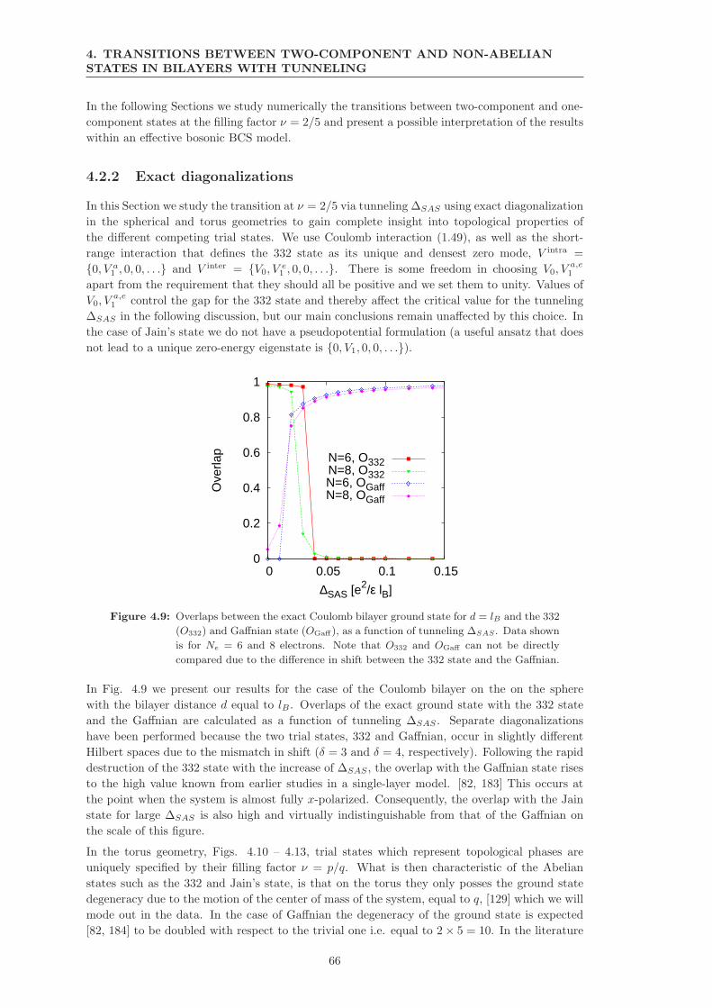
4. TRANSITIONS BETWEEN TWO-COMPONENT AND NON-ABELIAN
STATES IN BILAYERS WITH TUNNELING
In the following Sections we study numerically the transitions between two-component and one-
component states at the filling factor ν = 2/5 and present a possible interpretation of the results
within an effective bosonic BCS model.
4.2.2 Exact diagonalizations
In this Section we study the transition at ν = 2/5 via tunneling ∆SAS using exact diagonalization
in the spherical and torus geometries to gain complete insight into topological properties of
the different competing trial states. We use Coulomb interaction (1.49), as well as the short-
range interaction that defines the 332 state as its unique and densest zero mode, V intra =
0, V a1 , 0, 0, . . . and V inter = V0, V
e1 , 0, 0, . . .. There is some freedom in choosing V0, V
a,e1
apart from the requirement that they should all be positive and we set them to unity. Values of
V0, Va,e1 control the gap for the 332 state and thereby affect the critical value for the tunneling
∆SAS in the following discussion, but our main conclusions remain unaffected by this choice. In
the case of Jain’s state we do not have a pseudopotential formulation (a useful ansatz that does
not lead to a unique zero-energy eigenstate is 0, V1, 0, 0, . . .).
0
0.2
0.4
0.6
0.8
1
0 0.05 0.1 0.15
Ove
rlap
∆SAS [e2/ε lB]
N=6, O332N=8, O332N=6, OGaffN=8, OGaff
Figure 4.9: Overlaps between the exact Coulomb bilayer ground state for d = lB and the 332
(O332) and Gaffnian state (OGaff), as a function of tunneling ∆SAS . Data shown
is for Ne = 6 and 8 electrons. Note that O332 and OGaff can not be directly
compared due to the difference in shift between the 332 state and the Gaffnian.
In Fig. 4.9 we present our results for the case of the Coulomb bilayer on the on the sphere
with the bilayer distance d equal to lB . Overlaps of the exact ground state with the 332 state
and the Gaffnian are calculated as a function of tunneling ∆SAS . Separate diagonalizations
have been performed because the two trial states, 332 and Gaffnian, occur in slightly different
Hilbert spaces due to the mismatch in shift (δ = 3 and δ = 4, respectively). Following the rapid
destruction of the 332 state with the increase of ∆SAS , the overlap with the Gaffnian state rises
to the high value known from earlier studies in a single-layer model. [82, 183] This occurs at
the point when the system is almost fully x-polarized. Consequently, the overlap with the Jain
state for large ∆SAS is also high and virtually indistinguishable from that of the Gaffnian on
the scale of this figure.
In the torus geometry, Figs. 4.10 – 4.13, trial states which represent topological phases are
uniquely specified by their filling factor ν = p/q. What is then characteristic of the Abelian
states such as the 332 and Jain’s state, is that on the torus they only posses the ground state
degeneracy due to the motion of the center of mass of the system, equal to q, [129] which we will
mode out in the data. In the case of Gaffnian the degeneracy of the ground state is expected
[82, 184] to be doubled with respect to the trivial one i.e. equal to 2× 5 = 10. In the literature
66
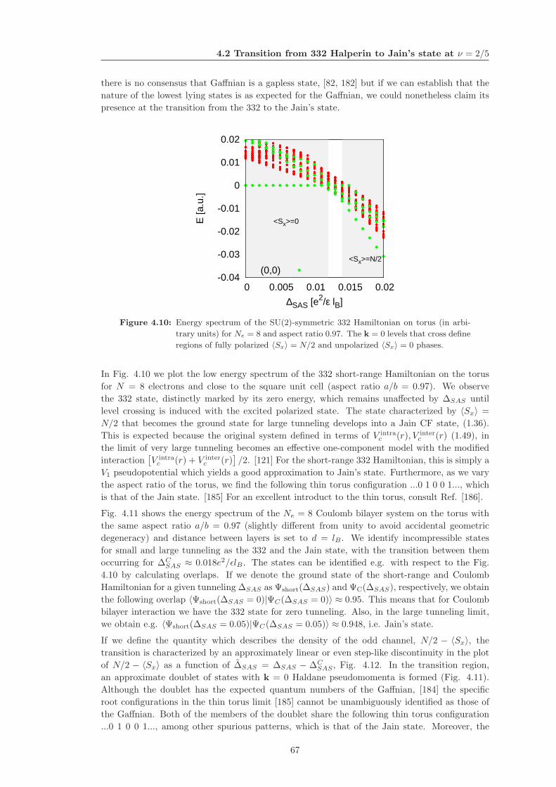
4.2 Transition from 332 Halperin to Jain’s state at ν = 2/5
there is no consensus that Gaffnian is a gapless state, [82, 182] but if we can establish that the
nature of the lowest lying states is as expected for the Gaffnian, we could nonetheless claim its
presence at the transition from the 332 to the Jain’s state.
-0.04
-0.03
-0.02
-0.01
0
0.01
0.02
0 0.005 0.01 0.015 0.02
E [a
.u.]
∆SAS [e2/ε lB]
(0,0)
<Sx>=0
<Sx>=N/2
Figure 4.10: Energy spectrum of the SU(2)-symmetric 332 Hamiltonian on torus (in arbi-
trary units) for Ne = 8 and aspect ratio 0.97. The k = 0 levels that cross define
regions of fully polarized 〈Sx〉 = N/2 and unpolarized 〈Sx〉 = 0 phases.
In Fig. 4.10 we plot the low energy spectrum of the 332 short-range Hamiltonian on the torus
for N = 8 electrons and close to the square unit cell (aspect ratio a/b = 0.97). We observe
the 332 state, distinctly marked by its zero energy, which remains unaffected by ∆SAS until
level crossing is induced with the excited polarized state. The state characterized by 〈Sx〉 =
N/2 that becomes the ground state for large tunneling develops into a Jain CF state, (1.36).
This is expected because the original system defined in terms of V intrac (r), V inter
c (r) (1.49), in
the limit of very large tunneling becomes an effective one-component model with the modified
interaction[
V intrac (r) + V inter
c (r)]
/2. [121] For the short-range 332 Hamiltonian, this is simply a
V1 pseudopotential which yields a good approximation to Jain’s state. Furthermore, as we vary
the aspect ratio of the torus, we find the following thin torus configuration ...0 1 0 0 1..., which
is that of the Jain state. [185] For an excellent introduct to the thin torus, consult Ref. [186].
Fig. 4.11 shows the energy spectrum of the Ne = 8 Coulomb bilayer system on the torus with
the same aspect ratio a/b = 0.97 (slightly different from unity to avoid accidental geometric
degeneracy) and distance between layers is set to d = lB . We identify incompressible states
for small and large tunneling as the 332 and the Jain state, with the transition between them
occurring for ∆CSAS ≈ 0.018e2/ǫlB . The states can be identified e.g. with respect to the Fig.
4.10 by calculating overlaps. If we denote the ground state of the short-range and Coulomb
Hamiltonian for a given tunneling ∆SAS as Ψshort(∆SAS) and ΨC(∆SAS), respectively, we obtain
the following overlap 〈Ψshort(∆SAS = 0)|ΨC(∆SAS = 0)〉 ≈ 0.95. This means that for Coulomb
bilayer interaction we have the 332 state for zero tunneling. Also, in the large tunneling limit,
we obtain e.g. 〈Ψshort(∆SAS = 0.05)|ΨC(∆SAS = 0.05)〉 ≈ 0.948, i.e. Jain’s state.
If we define the quantity which describes the density of the odd channel, N/2 − 〈Sx〉, the
transition is characterized by an approximately linear or even step-like discontinuity in the plot
of N/2 − 〈Sx〉 as a function of ∆SAS = ∆SAS − ∆CSAS , Fig. 4.12. In the transition region,
an approximate doublet of states with k = 0 Haldane pseudomomenta is formed (Fig. 4.11).
Although the doublet has the expected quantum numbers of the Gaffnian, [184] the specific
root configurations in the thin torus limit [185] cannot be unambiguously identified as those of
the Gaffnian. Both of the members of the doublet share the following thin torus configuration
...0 1 0 0 1..., among other spurious patterns, which is that of the Jain state. Moreover, the
67
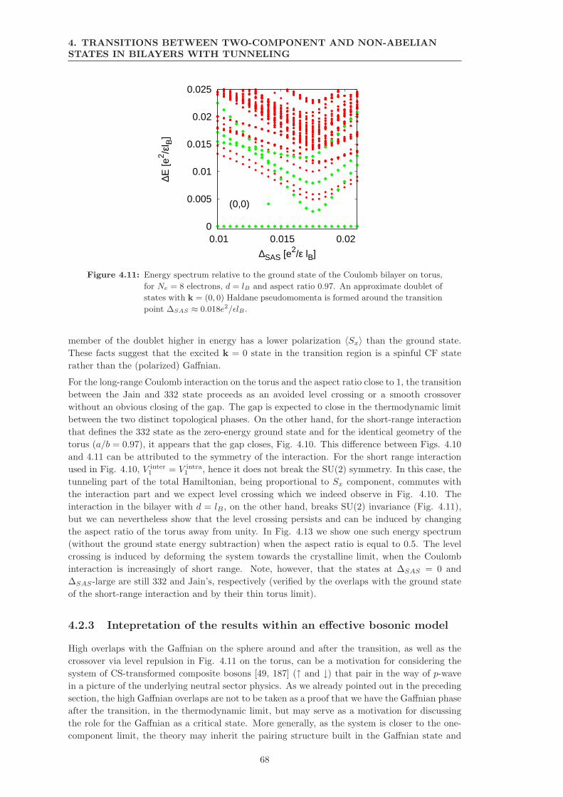
4. TRANSITIONS BETWEEN TWO-COMPONENT AND NON-ABELIAN
STATES IN BILAYERS WITH TUNNELING
0
0.005
0.01
0.015
0.02
0.025
0.01 0.015 0.02
∆E [e
2 /εl B
]
∆SAS [e2/ε lB]
(0,0)
Figure 4.11: Energy spectrum relative to the ground state of the Coulomb bilayer on torus,
for Ne = 8 electrons, d = lB and aspect ratio 0.97. An approximate doublet of
states with k = (0, 0) Haldane pseudomomenta is formed around the transition
point ∆SAS ≈ 0.018e2/ǫlB .
member of the doublet higher in energy has a lower polarization 〈Sx〉 than the ground state.
These facts suggest that the excited k = 0 state in the transition region is a spinful CF state
rather than the (polarized) Gaffnian.
For the long-range Coulomb interaction on the torus and the aspect ratio close to 1, the transition
between the Jain and 332 state proceeds as an avoided level crossing or a smooth crossover
without an obvious closing of the gap. The gap is expected to close in the thermodynamic limit
between the two distinct topological phases. On the other hand, for the short-range interaction
that defines the 332 state as the zero-energy ground state and for the identical geometry of the
torus (a/b = 0.97), it appears that the gap closes, Fig. 4.10. This difference between Figs. 4.10
and 4.11 can be attributed to the symmetry of the interaction. For the short range interaction
used in Fig. 4.10, V inter1 = V intra
1 , hence it does not break the SU(2) symmetry. In this case, the
tunneling part of the total Hamiltonian, being proportional to Sx component, commutes with
the interaction part and we expect level crossing which we indeed observe in Fig. 4.10. The
interaction in the bilayer with d = lB , on the other hand, breaks SU(2) invariance (Fig. 4.11),
but we can nevertheless show that the level crossing persists and can be induced by changing
the aspect ratio of the torus away from unity. In Fig. 4.13 we show one such energy spectrum
(without the ground state energy subtraction) when the aspect ratio is equal to 0.5. The level
crossing is induced by deforming the system towards the crystalline limit, when the Coulomb
interaction is increasingly of short range. Note, however, that the states at ∆SAS = 0 and
∆SAS-large are still 332 and Jain’s, respectively (verified by the overlaps with the ground state
of the short-range interaction and by their thin torus limit).
4.2.3 Intepretation of the results within an effective bosonic model
High overlaps with the Gaffnian on the sphere around and after the transition, as well as the
crossover via level repulsion in Fig. 4.11 on the torus, can be a motivation for considering the
system of CS-transformed composite bosons [49, 187] (↑ and ↓) that pair in the way of p-wave
in a picture of the underlying neutral sector physics. As we already pointed out in the preceding
section, the high Gaffnian overlaps are not to be taken as a proof that we have the Gaffnian phase
after the transition, in the thermodynamic limit, but may serve as a motivation for discussing
the role for the Gaffnian as a critical state. More generally, as the system is closer to the one-
component limit, the theory may inherit the pairing structure built in the Gaffnian state and
68
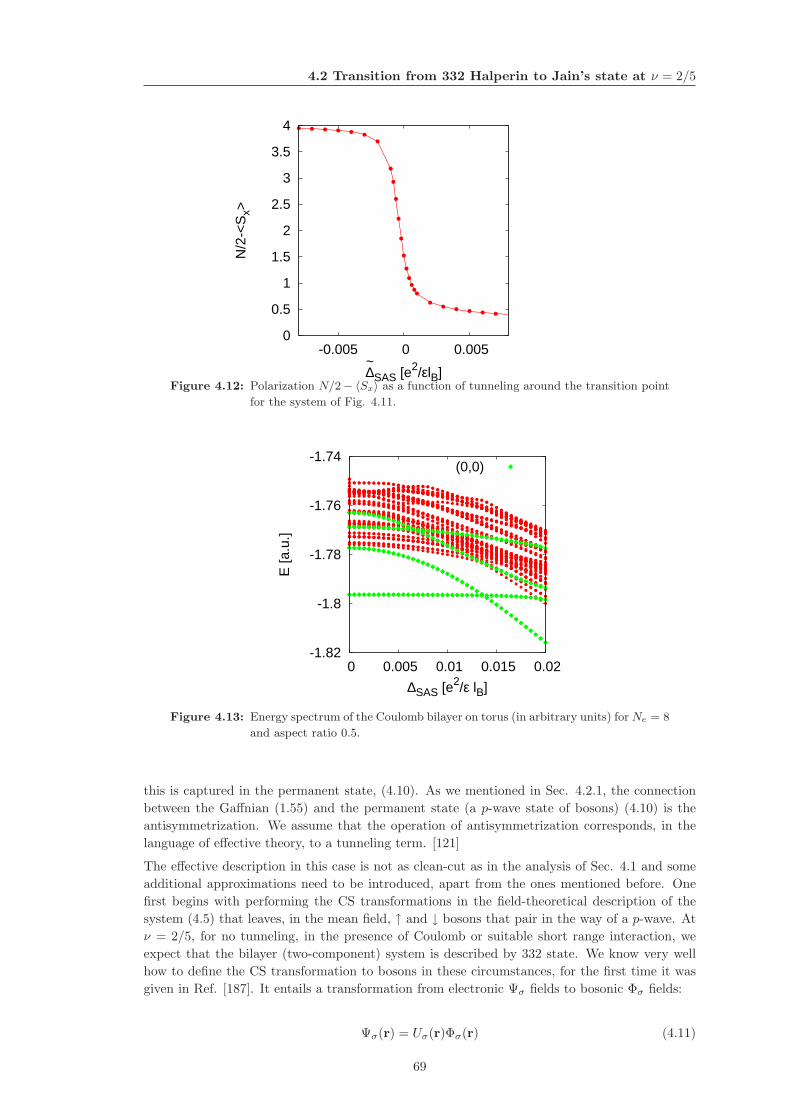
4.2 Transition from 332 Halperin to Jain’s state at ν = 2/5
0
0.5
1
1.5
2
2.5
3
3.5
4
-0.005 0 0.005
N/2
-<S
x>
∆~
SAS [e2/εlB]Figure 4.12: Polarization N/2− 〈Sx〉 as a function of tunneling around the transition point
for the system of Fig. 4.11.
-1.82
-1.8
-1.78
-1.76
-1.74
0 0.005 0.01 0.015 0.02
E [a
.u.]
∆SAS [e2/ε lB]
(0,0)
Figure 4.13: Energy spectrum of the Coulomb bilayer on torus (in arbitrary units) for Ne = 8
and aspect ratio 0.5.
this is captured in the permanent state, (4.10). As we mentioned in Sec. 4.2.1, the connection
between the Gaffnian (1.55) and the permanent state (a p-wave state of bosons) (4.10) is the
antisymmetrization. We assume that the operation of antisymmetrization corresponds, in the
language of effective theory, to a tunneling term. [121]
The effective description in this case is not as clean-cut as in the analysis of Sec. 4.1 and some
additional approximations need to be introduced, apart from the ones mentioned before. One
first begins with performing the CS transformations in the field-theoretical description of the
system (4.5) that leaves, in the mean field, ↑ and ↓ bosons that pair in the way of a p-wave. At
ν = 2/5, for no tunneling, in the presence of Coulomb or suitable short range interaction, we
expect that the bilayer (two-component) system is described by 332 state. We know very well
how to define the CS transformation to bosons in these circumstances, for the first time it was
given in Ref. [187]. It entails a transformation from electronic Ψσ fields to bosonic Φσ fields:
Ψσ(r) = Uσ(r)Φσ(r) (4.11)
69
4. TRANSITIONS BETWEEN TWO-COMPONENT AND NON-ABELIAN
STATES IN BILAYERS WITH TUNNELING
where
Uσ(r) = exp−i∫
dr′arg(r− r′)[3ρσ(r′) + 2ρ−σ(r′)] (4.12)
where arg(r − r′) is the angle the vector r − r′ forms with the x axis. In the mean field (when
the fluctuations of gauge fields are neglected) we, in fact, describe a system of ↑ and ↓ bosons
that interact. Therefore we have in the first approximation two ordinary Bose condensates. By
the virtue of the Anderson-Higgs mechanism i.e. gauge fluctuations, the two Goldstone modes
become gapped and the two gapped bosonic systems describe the two-component 332 system.
The complication comes when we consider the tunneling term as an extra perturbation and an
extra term in our starting Hamiltonian for the electrons. The tunneling term is
HT = −λ(
Ψ†↑(r)Ψ↓(r) + Ψ†
↓(r)Ψ↑(r))
, (4.13)
where λ denotes the tunneling amplitude in this section. Due to the CS transformation (4.11)
this can not be translated simply into the hopping of bosons because:
Ψ†σΨ−σ = Φ†
σU†σU−σΦ−σ (4.14)
and only in the mean field approximation for which
U†σU−σ ≈ I (4.15)
(where I is the identity) we have a simple tunneling of bosons i.e.
HT ≈ −λ(
Φ†↑(r)Φ↓(r) + h.c.
)
(4.16)
The necessary assumption in Eq.(4.15) is ρs = ρ↑(r) − ρ↓(r) ≈ 0 i.e. that the fluctuations in
density in ↑ parallel the ones in ↓, or the fluctuations in the pseudospin density are negligible.
This is a crucial approximation that reconciles the CS transformation with the tunneling term
and enables the similar analysis as in Sec. 4.1. Unfortunately, this approximation is difficult to
quantify, but nonetheless we expect to get the qualitatively correct insight into the transition.
Additional justification for the bosonic model arises from numerics. Namely, the results for SU(2)
symmetric interaction (4.10) and Coulomb interaction (4.11) both reflect the abrupt change in
polarization at the transition. In this case, we may use the SU(2)-invariant interaction as a
starting point and the symmetric-antisymmetric basis for the Chern-Simons transformation.
This way, the tunneling term will retain the same form as in the fermionic basis.
Treating the residual interaction in a mean field manner i.e. taking the Hartree-Fock and BCS
decomposition, we come to the following form of the Hamiltonian for the effective description of
↑ and ↓ bosons around the k = 0 point in the momentum space:
H =∑
k
(
∑
σ
ǫkb†kσbkσ − λ(b†k↑bk↓ + b†k↓bk↑) + ∆k b
†k↑b
†−k↓ + ∆∗
k b−k↓bk↑
)
(4.17)
where ǫk = ǫk − µ, σ =↑, ↓ and ∆k is the p-wave order parameter function ∆k ∼ kx − iky. The
question of mutual statistics (between ↑ and ↓ electrons and the ensuing composite bosons) may
be raised but we assume that it is bosonic. In Ref. [168] we show that the Hamiltonian above
can be diagonalized by a Bogoliubov transformation to obtain two pairs of eigenvalues:
E + λ,E − λ, and − E + λ,−E − λ, (4.18)
where E =√
ǫ2k − |∆k|2. The last two eigenvalues −E±λ correspond to well-defined excitations
of the system. For µ > 0:
− E ± λ ≈ −µ+ ǫk +∆2
2µ± λ (4.19)
i.e. we have an ordinary, non-interacting boson description where the tunneling λ defines the
transition at λ = µ from the two Bose condensates to a one Bose condensate (one disappears
70
4.3 Conclusions
because µeff = µ − λ < 0 i.e. we have vacuum for these particles). This motivates to consider
that a viable composite boson effective description of the ν = 2/5 Jain’s state is with only one
composite boson condensate and a Bose vacuum. This stems as a natural consequence from our
analysis and the multicomponent approach to Jain’s states. [117] Any effective description of
quantum Hall states must encompass the edge physics as the low energy physics of these states
happens on the edge. In the effective description based on composite bosons [50] of the ν = 2/5
fractional quantum Hall edge, one encounters both charge and neutral modes that propagate in
the same direction as relativistic particles and the discrepancy with respect to experiments [188]
has to be resolved [189]. In the effective description based on composite fermions, [190] at ν = 2/5
edge only the charge mode is propagating, in agreement with the experiment, but the reason why
the neutral mode does not propagate is not obvious. Here we suggest an effective picture of the
multicomponent degrees of freedom of Jain’s state at ν = 2/5 via a Bose vacuum. Any time we
have to describe an excitation of the system that involves also these, multicomponent, degrees
of freedom, we excite a boson in a vacuum that propagates, not relativistically, but according
to Schrodinger equation [191], which in an effective description can be neglected with respect to
the charge wave propagation along the edge.
Going back to the eigenvalue problem, one may consider the remaining pair of the eigenvalues:
E ± λ. (4.20)
It is then obvious from (4.19) that these excitations are unstable and hence may relate to the
excited states. In fact, it can be shown [168] that these excitations, in the long distance limit,
describe a permanent state (4.10), if we assume that the Hamiltonian H is regularized by a
phenomenological term H + λN . [121] Therefore before reaching the strong tunneling limit and
the incompressible FQH state connected with the single BCS condensate in this description at
ν = 2/5 (Jain’s state), we may find a state at the transition that evolves from an excited state
described by the permanent. It may appear mysterious why we choose the theory with pairing
to describe a transition which the numerics seem to suggest to occur between two Abelian states.
As we pointed out in Sec. 4.1, the formalism of Read and Green [171] also applies to the situation
where the pairing structure of the theory is reflected in what turns out to be the excited state
(such as the Pfaffian), whereas the ground state (i.e. CFL) has no pairing.
4.3 Conclusions
In Section 4.1 we investigated the possibility of creating the Moore-Read Pfaffian out of the paired
two-component 331 state via tunneling. Exact diagonalization, performed under the constraint
of the LLL projection and the fixed total number of particles, could not detect a stable Pfaffian
phase, but a critical one between 331 and CFL phases. While the short-range interaction is likely
to favor a direct transition from the 331 to the CFL phase, long-range Coulomb interactions leave
the possibility for a Pfaffian-like phase if the parameters of the system are tuned in a special
way. Based on the connection between our numerical results and the effective BCS Hamiltonian
theory of paired states, we argue that one way to stabilize the Pfaffian state is to change the
density (number of particles) of the system while increasing the tunneling.
The transition at ν = 2/5 is studied in the presence of Coulomb interaction appropriate for the
quantum Hall bilayer and a model short-ranged interaction appropriate for the 332 Halperin’s
state. We established an avoided level crossing in the first case and, in the latter, a first order
transition. With respect to the appearance of the Gaffnian state in the transition region between
332 and Jain, we can conclude that in finite systems this is only possible for the interaction that
breaks SU(2) invariance, like the Coulomb bilayer interaction, but remains an unlikely possibility
because of the difficulty in establishing the thin torus limit for the approximate k = 0 doublet
found for the torus with the aspect ratio close to unity (Fig. 4.11). Within the effective bosonic
model, we find that the transition in the presence of the Coulomb interaction may be viewed as
71
4. TRANSITIONS BETWEEN TWO-COMPONENT AND NON-ABELIAN
STATES IN BILAYERS WITH TUNNELING
a transition from two Bose condensates to a Bose condensate and a Bose vacuum, as one type of
bosons gradually disappears from the system. The outcome, with the Bose vacuum, can serve
as an effective description of the Jain state.
72
Chapter 5
Wide quantum wells
In this Chapter we explore multicomponent and non-Abelian states in wide quantum wells.
The first system we analyze in Sec. 5.1 is a single QH layer with finite thickness. We model
the thickness by the Zhang-Das Sarma (ZDS) potential and find quantum phase transitions
between compressible and incompressible states as the parameter of the ZDS interaction is var-
ied. In particular, we show that incompressible ground states evolve adiabatically under tuning
the parameter of ZDS interaction, whereas the compressible ones are driven through a phase
transition. Overlap calculations show that the resulting phase is increasingly well described
by appropriate analytic model wave functions (Laughlin, Moore-Read, Read-Rezayi). This sce-
nario is shared by both odd (ν = 1/3, 1/5, 3/5, 7/3, 11/5, 13/5) and even denominator states
(ν = 1/2, 1/4, 5/2, 9/4). In particular, the Fermi liquid-like state at ν = 1/2 gives way, at large
enough value of the width parameter, to an incompressible state identified as the Moore-Read
Pfaffian on the basis of its entanglement spectrum. The second system we analyze (Sec. 5.2) is
explicitly a two-component model of the quantum well which takes into account the two low-
est subbands. We make a direct connection between this model of the quantum well and the
effective-bilayer model. We focus on the filling factors ν = 1/2 and ν = 1/4. In the case of
former, we explore the transition between the 331 state and the Moore-Read Pfaffian, subject
of Chapter 4. At ν = 1/4 we investigate the nature of the ground state examining different
multicomponent candidates (553, 771, Haldane-Rezayi state) and the generalized Moore-Read
Pfaffian. This Chapter contains some unpublished results and summarizes the main findings of
Refs. [133] and [140].
5.1 Finite thickness and phase transitions between com-
pressible and incompressible states
As a warm-up to the realistic quantum well model that is the subject of Sec. 5.2, here we address,
via large-scale ED calculations on finite spheres, the important and interesting question of how
to tune various FQH ground states between ungapped compressible and gapped incompressible
phases by continuously varying the effective electron-electron interaction in a single QH layer.
We show that a simple single-parameter parametrization of the effective interaction through the
ZDS model (1.17) provides a flexible and powerful method of studying quantum phase transitions
(QPTs) between compressible and incompressible phases at both even and odd-denominator
FQH states. ZDS interaction (1.17) for the quantum well of width w
V (r, w) =e2
ǫ√r2 + w2
, (5.1)
possesses a rich structure that can drive the system from parameter regions where it appears
to be compressible (manifested by the ground state that breaks rotational invariance i.e. the
73
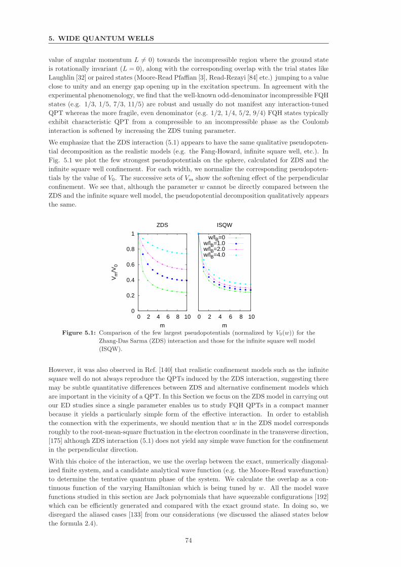
5. WIDE QUANTUM WELLS
value of angular momentum L 6= 0) towards the incompressible region where the ground state
is rotationally invariant (L = 0), along with the corresponding overlap with the trial states like
Laughlin [32] or paired states (Moore-Read Pfaffian [3], Read-Rezayi [84] etc.) jumping to a value
close to unity and an energy gap opening up in the excitation spectrum. In agreement with the
experimental phenomenology, we find that the well-known odd-denominator incompressible FQH
states (e.g. 1/3, 1/5, 7/3, 11/5) are robust and usually do not manifest any interaction-tuned
QPT whereas the more fragile, even denominator (e.g. 1/2, 1/4, 5/2, 9/4) FQH states typically
exhibit characteristic QPT from a compressible to an incompressible phase as the Coulomb
interaction is softened by increasing the ZDS tuning parameter.
We emphasize that the ZDS interaction (5.1) appears to have the same qualitative pseudopoten-
tial decomposition as the realistic models (e.g. the Fang-Howard, infinite square well, etc.). In
Fig. 5.1 we plot the few strongest pseudopotentials on the sphere, calculated for ZDS and the
infinite square well confinement. For each width, we normalize the corresponding pseudopoten-
tials by the value of V0. The successive sets of Vm show the softening effect of the perpendicular
confinement. We see that, although the parameter w cannot be directly compared between the
ZDS and the infinite square well model, the pseudopotential decomposition qualitatively appears
the same.
0
0.2
0.4
0.6
0.8
1
0 2 4 6 8 10
Vm
/V0
m
ZDS
0 2 4 6 8 10
m
ISQW
w/lB=0w/lB=1.0w/lB=2.0w/lB=4.0
Figure 5.1: Comparison of the few largest pseudopotentials (normalized by V0(w)) for the
Zhang-Das Sarma (ZDS) interaction and those for the infinite square well model
(ISQW).
However, it was also observed in Ref. [140] that realistic confinement models such as the infinite
square well do not always reproduce the QPTs induced by the ZDS interaction, suggesting there
may be subtle quantitative differences between ZDS and alternative confinement models which
are important in the vicinity of a QPT. In this Section we focus on the ZDS model in carrying out
our ED studies since a single parameter enables us to study FQH QPTs in a compact manner
because it yields a particularly simple form of the effective interaction. In order to establish
the connection with the experiments, we should mention that w in the ZDS model corresponds
roughly to the root-mean-square fluctuation in the electron coordinate in the transverse direction,
[175] although ZDS interaction (5.1) does not yield any simple wave function for the confinement
in the perpendicular direction.
With this choice of the interaction, we use the overlap between the exact, numerically diagonal-
ized finite system, and a candidate analytical wave function (e.g. the Moore-Read wavefunction)
to determine the tentative quantum phase of the system. We calculate the overlap as a con-
tinuous function of the varying Hamiltonian which is being tuned by w. All the model wave
functions studied in this section are Jack polynomials that have squeezable configurations [192]
which can be efficiently generated and compared with the exact ground state. In doing so, we
disregard the aliased cases [133] from our considerations (we discussed the aliased states below
the formula 2.4).
74
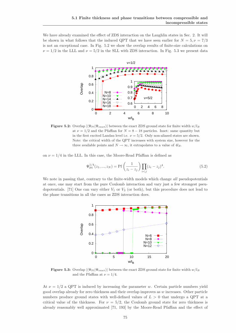
5.1 Finite thickness and phase transitions between compressible and
incompressible states
We have already examined the effect of ZDS interaction on the Laughlin states in Sec. 2. It will
be shown in what follows that the induced QPT that we have seen earlier for N = 5, ν = 7/3
is not an exceptional case. In Fig. 5.2 we show the overlap results of finite-size calculations on
ν = 1/2 in the LLL and ν = 5/2 in the SLL with ZDS interaction. In Fig. 5.3 we present data
0
0.2
0.4
0.6
0.8
1
0 2 4 6 8 10
Ove
rlap
w/lB
ν=1/2
N=8N=10N=14N=16N=18
0.6
0.7
0.8
0.9
1
0 2 4 6 8
ν=5/2
Figure 5.2: Overlap |〈ΨPf |Ψexact〉| between the exact ZDS ground state for finite width w/lBat ν = 1/2 and the Pfaffian for N = 8 − 18 particles. Inset: same quantity but
in the first excited Landau level i.e. ν = 5/2. Only non-aliased states are shown.
Note: the critical width of the QPT increases with system size, however for the
three available points and N → ∞, it extrapolates to a value of 4lB .
on ν = 1/4 in the LLL. In this case, the Moore-Read Pfaffian is defined as
Ψ1/4Pf (z1, ..., zN ) = Pf
(
1
zi − zj
)
∏
i<j
(zi − zj)4. (5.2)
We note in passing that, contrary to the finite-width models which change all pseudopotentials
at once, one may start from the pure Coulomb interaction and vary just a few strongest pseu-
dopotentials. [71] One can vary either V1 or V3 (or both), but this procedure does not lead to
the phase transitions in all the cases as ZDS interaction does.
0
0.2
0.4
0.6
0.8
1
0 5 10 15 20
Ove
rlap
w/lB
N=6N=8
N=10N=12
Figure 5.3: Overlap |〈ΨPf |Ψexact〉| between the exact ZDS ground state for finite width w/lBand the Pfaffian at ν = 1/4.
At ν = 1/2 a QPT is induced by increasing the parameter w. Certain particle numbers yield
good overlap already for zero thickness and their overlap improves as w increases. Other particle
numbers produce ground states with well-defined values of L > 0 that undergo a QPT at a
critical value of the thickness. For ν = 5/2, the Coulomb ground state for zero thickness is
already reasonably well approximated [71, 193] by the Moore-Read Pfaffian and the effect of
75
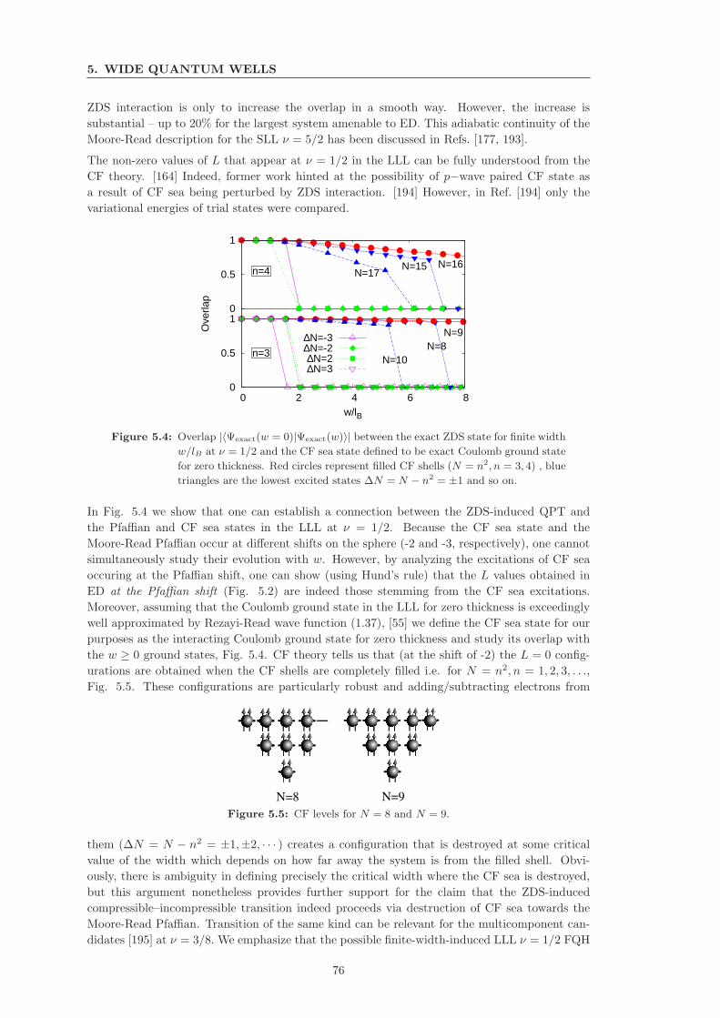
5. WIDE QUANTUM WELLS
ZDS interaction is only to increase the overlap in a smooth way. However, the increase is
substantial – up to 20% for the largest system amenable to ED. This adiabatic continuity of the
Moore-Read description for the SLL ν = 5/2 has been discussed in Refs. [177, 193].
The non-zero values of L that appear at ν = 1/2 in the LLL can be fully understood from the
CF theory. [164] Indeed, former work hinted at the possibility of p−wave paired CF state as
a result of CF sea being perturbed by ZDS interaction. [194] However, in Ref. [194] only the
variational energies of trial states were compared.
0
0.5
10
0.5
1
0 2 4 6 8
Ove
rlap
w/lB
∆N=-3∆N=-2∆N=2∆N=3
n=4
n=3
N=16N=15N=17
N=9N=8
N=10
Figure 5.4: Overlap |〈Ψexact(w = 0)|Ψexact(w)〉| between the exact ZDS state for finite width
w/lB at ν = 1/2 and the CF sea state defined to be exact Coulomb ground state
for zero thickness. Red circles represent filled CF shells (N = n2, n = 3, 4) , blue
triangles are the lowest excited states ∆N = N − n2 = ±1 and so on.
In Fig. 5.4 we show that one can establish a connection between the ZDS-induced QPT and
the Pfaffian and CF sea states in the LLL at ν = 1/2. Because the CF sea state and the
Moore-Read Pfaffian occur at different shifts on the sphere (-2 and -3, respectively), one cannot
simultaneously study their evolution with w. However, by analyzing the excitations of CF sea
occuring at the Pfaffian shift, one can show (using Hund’s rule) that the L values obtained in
ED at the Pfaffian shift (Fig. 5.2) are indeed those stemming from the CF sea excitations.
Moreover, assuming that the Coulomb ground state in the LLL for zero thickness is exceedingly
well approximated by Rezayi-Read wave function (1.37), [55] we define the CF sea state for our
purposes as the interacting Coulomb ground state for zero thickness and study its overlap with
the w ≥ 0 ground states, Fig. 5.4. CF theory tells us that (at the shift of -2) the L = 0 config-
urations are obtained when the CF shells are completely filled i.e. for N = n2, n = 1, 2, 3, . . .,
Fig. 5.5. These configurations are particularly robust and adding/subtracting electrons from
Figure 5.5: CF levels for N = 8 and N = 9.
them (∆N = N − n2 = ±1,±2, · · · ) creates a configuration that is destroyed at some critical
value of the width which depends on how far away the system is from the filled shell. Obvi-
ously, there is ambiguity in defining precisely the critical width where the CF sea is destroyed,
but this argument nonetheless provides further support for the claim that the ZDS-induced
compressible–incompressible transition indeed proceeds via destruction of CF sea towards the
Moore-Read Pfaffian. Transition of the same kind can be relevant for the multicomponent can-
didates [195] at ν = 3/8. We emphasize that the possible finite-width-induced LLL ν = 1/2 FQH
76
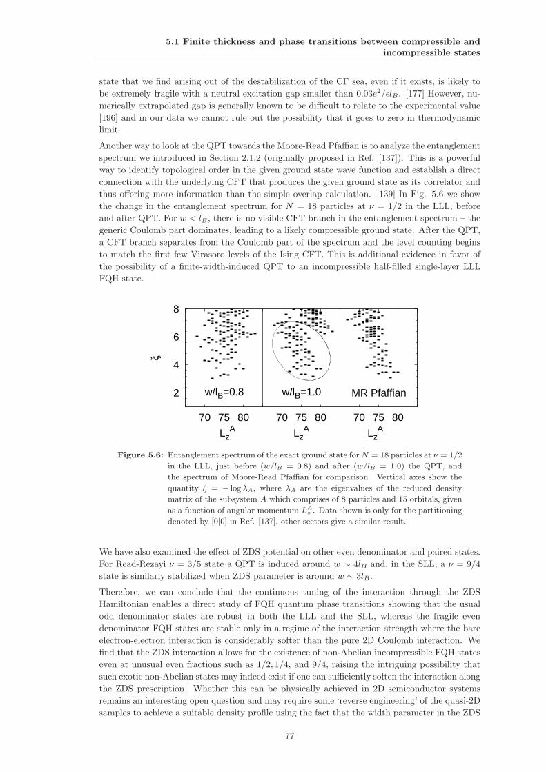
5.1 Finite thickness and phase transitions between compressible and
incompressible states
state that we find arising out of the destabilization of the CF sea, even if it exists, is likely to
be extremely fragile with a neutral excitation gap smaller than 0.03e2/ǫlB . [177] However, nu-
merically extrapolated gap is generally known to be difficult to relate to the experimental value
[196] and in our data we cannot rule out the possibility that it goes to zero in thermodynamic
limit.
Another way to look at the QPT towards the Moore-Read Pfaffian is to analyze the entanglement
spectrum we introduced in Section 2.1.2 (originally proposed in Ref. [137]). This is a powerful
way to identify topological order in the given ground state wave function and establish a direct
connection with the underlying CFT that produces the given ground state as its correlator and
thus offering more information than the simple overlap calculation. [139] In Fig. 5.6 we show
the change in the entanglement spectrum for N = 18 particles at ν = 1/2 in the LLL, before
and after QPT. For w < lB , there is no visible CFT branch in the entanglement spectrum – the
generic Coulomb part dominates, leading to a likely compressible ground state. After the QPT,
a CFT branch separates from the Coulomb part of the spectrum and the level counting begins
to match the first few Virasoro levels of the Ising CFT. This is additional evidence in favor of
the possibility of a finite-width-induced QPT to an incompressible half-filled single-layer LLL
FQH state.
2
4
6
8
70 75 80 70 75 80 70 75 80
ξ
LzA Lz
A LzA
w/lB=0.8 w/lB=1.0 MR Pfaffian
Figure 5.6: Entanglement spectrum of the exact ground state for N = 18 particles at ν = 1/2
in the LLL, just before (w/lB = 0.8) and after (w/lB = 1.0) the QPT, and
the spectrum of Moore-Read Pfaffian for comparison. Vertical axes show the
quantity ξ = − log λA, where λA are the eigenvalues of the reduced density
matrix of the subsystem A which comprises of 8 particles and 15 orbitals, given
as a function of angular momentum LAz . Data shown is only for the partitioning
denoted by [0|0] in Ref. [137], other sectors give a similar result.
We have also examined the effect of ZDS potential on other even denominator and paired states.
For Read-Rezayi ν = 3/5 state a QPT is induced around w ∼ 4lB and, in the SLL, a ν = 9/4
state is similarly stabilized when ZDS parameter is around w ∼ 3lB .
Therefore, we can conclude that the continuous tuning of the interaction through the ZDS
Hamiltonian enables a direct study of FQH quantum phase transitions showing that the usual
odd denominator states are robust in both the LLL and the SLL, whereas the fragile even
denominator FQH states are stable only in a regime of the interaction strength where the bare
electron-electron interaction is considerably softer than the pure 2D Coulomb interaction. We
find that the ZDS interaction allows for the existence of non-Abelian incompressible FQH states
even at unusual even fractions such as 1/2, 1/4, and 9/4, raising the intriguing possibility that
such exotic non-Abelian states may indeed exist if one can sufficiently soften the interaction along
the ZDS prescription. Whether this can be physically achieved in 2D semiconductor systems
remains an interesting open question and may require some ‘reverse engineering’ of the quasi-2D
samples to achieve a suitable density profile using the fact that the width parameter in the ZDS
77
5. WIDE QUANTUM WELLS
model corresponds roughly to the variance of the electron position in the transverse direction.
5.2 Two-subband model of the quantum well
In the preceding Section we used a simple, one-component model of the wide quantum well.
In this Section we will introduce a realistic model that takes into account the two lowest sub-
bands as the relevant low-energy degrees of freedom available to the electrons. We consider an
infinite square well of width w in the direction z ∈ [0, w], Fig. 1.4. The electronic motion in
the z-direction will then be quantized, yielding an electronic subband structure. Instead of a
full description with all the electronic subbands, we only consider the two lowest subbands (we
comment on the validity of two-subband approximation in Sec. 5.2.1). We identify the two
subbands with the two pseudospin states, Ψ↑,↓ = φ↑,↓(z)YNφ/2,Nφ/2,m(θ, φ), where φ↑,↓ were
defined in (1.48) but we now label them as ↑ and ↓, instead of by their reflection symmetry
property (symmetric and antisymmetric, respectively). Y ’s represent monopole spherical har-
monics with −Nφ/2 ≤ m ≤ Nφ/2 (we assume that the states are entirely within the LLL). If the
energy splitting between the subbands is denoted by ∆SAS , the corresponding second quantized
Hamiltonian is given by [197]
H = −∆SASSz −∆ρSx +1
2
∑
m
∑
σV σ1σ2σ3σ4
m1,m2,m3,m4c†m1σ1
c†m2σ2cm4σ4
cm3σ3, (5.3)
where the first term stands for the Zeeman splitting between the subbands, followed by the
term which represents the density imbalance ∆ρ. For the infinite square well, ∆SAS is directly
determined by the width of the well w, however it is expected to be renormalized in each sample,
so it is convenient to think of it as a free parameter.
The matrix elements V σ1,σ2,σ3,σ4m1,m2,m3,m4
can be evaluated from the Haldane pseudopotentials for the
effective in-plane interaction
V σ1,σ2,σ3,σ4
2D (r1 − r2) =e2
ǫlB
∫
dz1
∫
dz2φ∗σ1
(z1)φ∗σ2
(z2)φσ3(z1)φσ4
(z2)√
|r1 − r2|2 + (z1 − z2)2, (5.4)
where the position variables are expressed in units of lB such that the integral is dimensionless.
To evaluate the pseudopotentials for the effective interaction (5.4) we sample the pseudopoten-
tials for the interaction 1/√r2 + z2 for many values of z and then use numerical interpolation
scheme to perform the integral over z variables.
As we are interested in the possible phases that may occur and the transitions between them, we
expect the model described by the Hamiltonian (5.3) to be qualitatively correct and in agreement
with other confinement models (e.g. the Fang-Howard, (1.14)) that assume the lowest subband
to be symmetric and the first excited one to have a node. Any difference of the confining potential
away from the infinite square well will modify the energy eigenvalues and the associated wave
functions φσ(z). However, it is expected that the energies are more strongly affected than the
wave functions. In particular, the nodal structure of the wave functions is robust, such that the
two lowest eigenstates of the infinite well faithfully represent the underlying features. However,
we will allow for the general values of the level splitting ∆SAS to account for the variations in
the eigen-energies.
5.2.1 Connection between the quantum-well model and the bilayer
The wide quantum well allows the electrons to reduce their mutual Coulomb repulsion by explor-
ing more efficiently the z-direction, and it has been argued that due to this effect, a spontaneous
bilayer may be formed, under appropriate conditions. [106, 109] Here, a connection is made
between both two-component models, on the basis of the Hamiltonian (5.3). We consider the
78
5.2 Two-subband model of the quantum well
quantum well to be symmetric around w/2, i.e. the lowest subband (↑) state is symmetric, and
the first excited one (↓) is antisymmetric. Furthermore, we consider, in this section, the electrons
to be in the 2D plane, for illustration reasons, although the conclusions remain valid also in the
spherical geometry.
The interaction part of the Hamiltonian (5.3) may be rewritten in terms of the density and spin-
density operators projected to a single Landau level. The Fourier components of the projected
density operator of pseudospin-σ electrons reads
ρσ(q) =∑
m,m′
⟨
m∣
∣e−iq·R∣∣m′⟩ c†mσcm′σ ,
in terms of the 2D wave vector q and the guiding-center operator R, the latter acting on the
states labeled by the quantum numbers m. It is furthermore useful to define the total (projected)
density operator
ρ(q) = ρ↑(q) + ρ↓(q) (5.5)
and the projected pseudospin density operators,
Sµ(q) =∑
m,m′
⟨
m∣
∣e−iq·R∣∣m′⟩ c†mσ
τµσ,σ′
2cm′σ′ , (5.6)
where τµσ,σ′ are the usual 2× 2 Pauli matrices with µ = x, y, z.
Using (5.5) and (5.6), we can organize the terms in the Hamiltonian (5.3) into density-density
interaction and terms beyond, which may be described as a spin-spin interaction. Indeed, the
density-density part consists of the effective interactions (5.4) V ↑↑↑↑2D , V ↓↓↓↓
2D , and V ↑↓↑↓2D = V ↓↑↓↑
2D .
Notice that the interactions in the first excited subband (↓) are generally weaker than in the
lowest one (↓) because the wave function φ↓(z) possesses a node at w/2, in the center of the
well, i.e. V ↑↑↑↑2D > V ↓↓↓↓
2D . With the help of the (spin) density operators (5.5) and (5.6), the
density-density part of the interaction Hamiltonian reads
Hρ−ρ =1
2
∑
q
VSU(2)(q)ρ(−q)ρ(q) + 2∑
q
V zsb(q)Sz(−q)Sz(q) +
∑
q
V zB(q)ρ(−q)Sz(q), (5.7)
in terms of the SU(2)-symmetric interaction
VSU(2)(q) =1
4
[
V ↑↑↑↑2D (q) + V ↓↓↓↓
2D (q) + 2V ↑↓↑↓2D (q)
]
, (5.8)
and the SU(2)-symmetry breaking interaction terms
V zsb(q) =
1
4
[
V ↑↑↑↑2D (q) + V ↓↓↓↓
2D (q)− 2V ↑↓↑↓2D (q)
]
(5.9)
and
V zB(q) =
1
2
[
V ↑↑↑↑2D (q)− V ↓↓↓↓
2D (q)]
. (5.10)
The remaining 12 interaction terms, which cannot be treated as density-density interactions, fall
into two different classes; the 8 terms with three equal spin orientations σ and one opposite −σare zero due to the antisymmetry of the integrand in Eq. (5.4). The remaining 4 interaction
terms with two ↑-spins and two ↓-spins are all equal due to the symmetry of the quantum well
around w/2,
V xsb ≡ V ↑↑↓↓
2D = V ↓↓↑↑2D = V ↑↓↓↑
2D = V ↓↑↑↓2D . (5.11)
They yield the term
Hzsb = 2
∑
q
V xsb(q)Sx(−q)Sx(q) , (5.12)
which needs to be added to the interaction Hamiltonian (5.7), as well as the term
HSAS = −∆SAS Sz(q = 0) , (5.13)
79
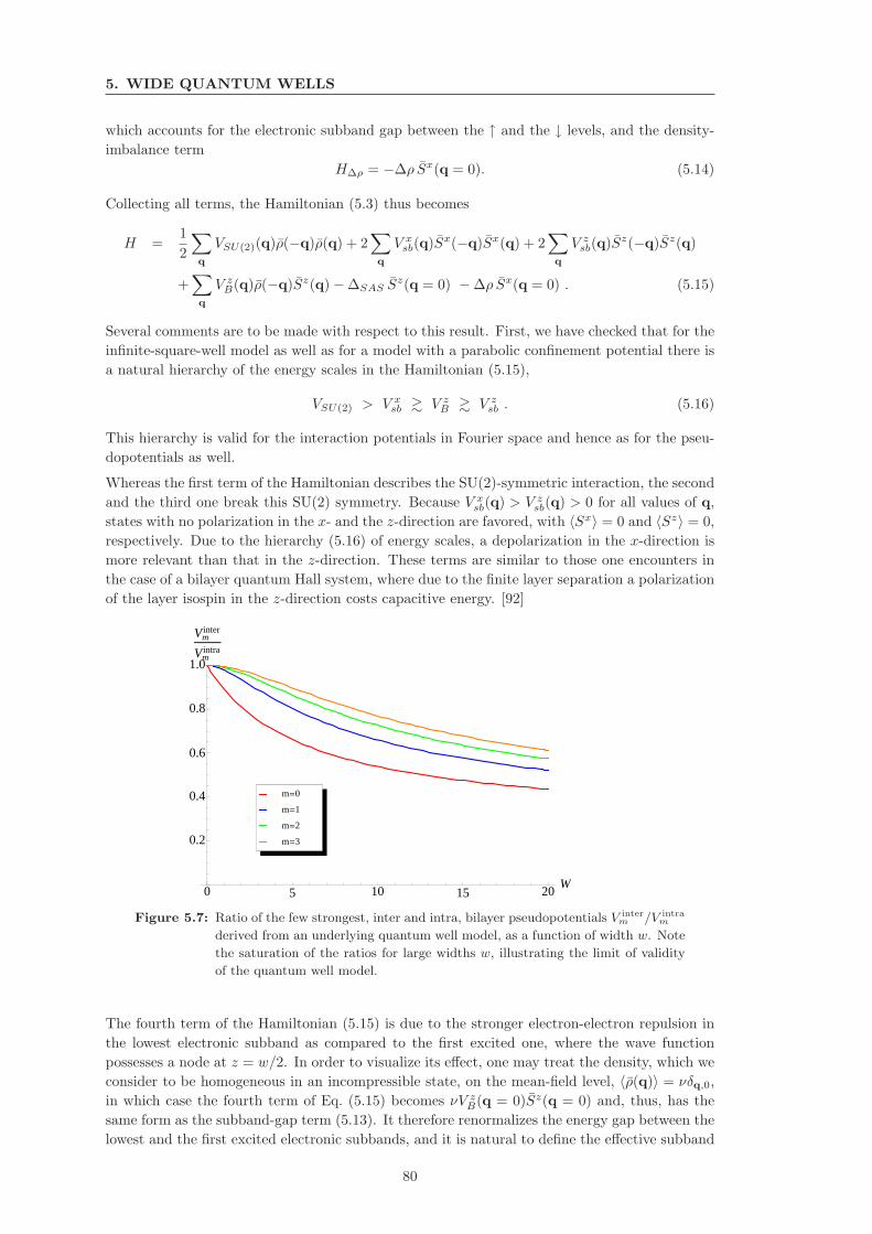
5. WIDE QUANTUM WELLS
which accounts for the electronic subband gap between the ↑ and the ↓ levels, and the density-
imbalance term
H∆ρ = −∆ρ Sx(q = 0). (5.14)
Collecting all terms, the Hamiltonian (5.3) thus becomes
H =1
2
∑
q
VSU(2)(q)ρ(−q)ρ(q) + 2∑
q
V xsb(q)Sx(−q)Sx(q) + 2
∑
q
V zsb(q)Sz(−q)Sz(q)
+∑
q
V zB(q)ρ(−q)Sz(q)−∆SAS S
z(q = 0) −∆ρ Sx(q = 0) . (5.15)
Several comments are to be made with respect to this result. First, we have checked that for the
infinite-square-well model as well as for a model with a parabolic confinement potential there is
a natural hierarchy of the energy scales in the Hamiltonian (5.15),
VSU(2) > V xsb & V z
B & V zsb . (5.16)
This hierarchy is valid for the interaction potentials in Fourier space and hence as for the pseu-
dopotentials as well.
Whereas the first term of the Hamiltonian describes the SU(2)-symmetric interaction, the second
and the third one break this SU(2) symmetry. Because V xsb(q) > V z
sb(q) > 0 for all values of q,
states with no polarization in the x- and the z-direction are favored, with 〈Sx〉 = 0 and 〈Sz〉 = 0,
respectively. Due to the hierarchy (5.16) of energy scales, a depolarization in the x-direction is
more relevant than that in the z-direction. These terms are similar to those one encounters in
the case of a bilayer quantum Hall system, where due to the finite layer separation a polarization
of the layer isospin in the z-direction costs capacitive energy. [92]
0 5 10 15 20W
0.2
0.4
0.6
0.8
1.0
Vminter
Vmintra
m=3
m=2
m=1
m=0
Figure 5.7: Ratio of the few strongest, inter and intra, bilayer pseudopotentials V interm /V intra
m
derived from an underlying quantum well model, as a function of width w. Note
the saturation of the ratios for large widths w, illustrating the limit of validity
of the quantum well model.
The fourth term of the Hamiltonian (5.15) is due to the stronger electron-electron repulsion in
the lowest electronic subband as compared to the first excited one, where the wave function
possesses a node at z = w/2. In order to visualize its effect, one may treat the density, which we
consider to be homogeneous in an incompressible state, on the mean-field level, 〈ρ(q)〉 = νδq,0,
in which case the fourth term of Eq. (5.15) becomes νV zB(q = 0)Sz(q = 0) and, thus, has the
same form as the subband-gap term (5.13). It therefore renormalizes the energy gap between the
lowest and the first excited electronic subbands, and it is natural to define the effective subband
80
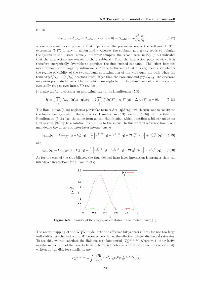
5.2 Two-subband model of the quantum well
gap as
∆SAS → ∆SAS = ∆SAS − νV zB(q = 0) = ∆SAS − γν
e2
ǫlB
w
lB, (5.17)
where γ is a numerical prefactor that depends on the precise nature of the well model. The
expression (5.17) is easy to understand – whereas the subband gap ∆SAS tends to polarize
the system in the ↑ state, namely in narrow samples, the second term in Eq. (5.17) indicates
that the interactions are weaker in the ↓ subband. From the interaction point of view, it is
therefore energetically favorable to populate the first excited subband. This effect becomes
more pronounced in larger quantum wells. Notice furthermore that this argument also delimits
the regime of validity of the two-subband approximation of the wide quantum well; when the
term γν(e2/ǫlB)× (w/lB) becomes much larger than the bare subband gap ∆SAS , the electrons
may even populate higher subbands, which are neglected in the present model, and the system
eventually crosses over into a 3D regime.
It is also useful to consider an approximation to the Hamiltonian (5.3)
H ≃ 1
2
∑
q
VSU(2)(q)ρ(−q)ρ(q) + 2∑
q
V xsb(q)Sx(−q)Sx(q)− ∆SASS
z(q = 0). (5.18)
The Hamiltonian (5.18) neglects a particular term ∝ Sz(−q)Sz(q), which turns out to constitute
the lowest energy scale in the interaction Hamiltonian (5.3) [see Eq. (5.16)]. Notice that the
Hamiltonian (5.18) has the same form as the Hamiltonian which describes a bilayer quantum
Hall system, [92] up to a rotation from the z- to the x-axis. In this rotated reference frame, one
may define the intra- and inter-layer interactions as
Vintra(q) = VSU(2)(q) + V xsb(q) =
1
4
[
V ↑↑↑↑2D (q) + V ↓↓↓↓
2D (q) + 2V ↑↓↑↓2D (q)
]
+ V ↑↑↓↓2D (q) (5.19)
and
Vinter(q) = VSU(2)(q)− V xsb(q) =
1
4
[
V ↑↑↑↑2D (q) + V ↓↓↓↓
2D (q) + 2V ↑↓↑↓2D (q)
]
− V ↑↑↓↓2D (q) . (5.20)
As for the case of the true bilayer, the thus defined intra-layer interaction is stronger than the
inter-layer interaction, for all values of q.
0
0.5
1
1.5
2
2.5
3
3.5
0 0.2 0.4 0.6 0.8 1
|φ(z
)|2
z
|+>|->
Figure 5.8: Densities of the single-particle states in the rotated frame, |±〉.
The above mapping of the WQW model onto the effective bilayer works best for not too large
well widths. As the well width W becomes very large, the effective bilayer distance d saturates.
To see this, we can calculate the Haldane pseudopotentials V σ1σ2σ3σ4m , where m is the relative
angular momentum of the two electrons. The pseudopotentials for the effective interaction (5.4),
written on the disk for simplicity, are
V σ1σ2σ3σ4
m =
∫
d2k
(2π)2e−k2
Lm(k2)V σ1σ2σ3σ4
2D (k),
81
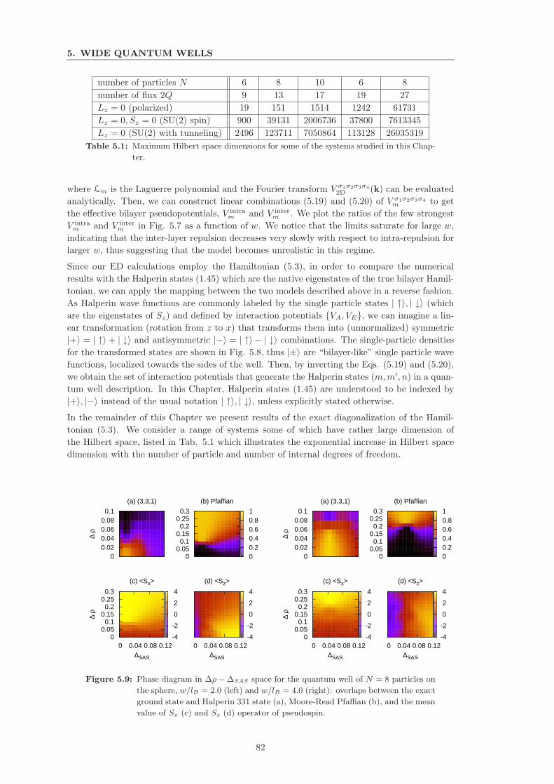
5. WIDE QUANTUM WELLS
number of particles N 6 8 10 6 8
number of flux 2Q 9 13 17 19 27
Lz = 0 (polarized) 19 151 1514 1242 61731
Lz = 0, Sz = 0 (SU(2) spin) 900 39131 2006736 37800 7613345
Lz = 0 (SU(2) with tunneling) 2496 123711 7050864 113128 26035319
Table 5.1: Maximum Hilbert space dimensions for some of the systems studied in this Chap-
ter.
where Lm is the Laguerre polynomial and the Fourier transform V σ1σ2σ3σ4
2D (k) can be evaluated
analytically. Then, we can construct linear combinations (5.19) and (5.20) of V σ1σ2σ3σ4m to get
the effective bilayer pseudopotentials, V intram and V inter
m . We plot the ratios of the few strongest
V intram and V inter
m in Fig. 5.7 as a function of w. We notice that the limits saturate for large w,
indicating that the inter-layer repulsion decreases very slowly with respect to intra-repulsion for
larger w, thus suggesting that the model becomes unrealistic in this regime.
Since our ED calculations employ the Hamiltonian (5.3), in order to compare the numerical
results with the Halperin states (1.45) which are the native eigenstates of the true bilayer Hamil-
tonian, we can apply the mapping between the two models described above in a reverse fashion.
As Halperin wave functions are commonly labeled by the single particle states | ↑〉, | ↓〉 (which
are the eigenstates of Sz) and defined by interaction potentials VA, VE, we can imagine a lin-
ear transformation (rotation from z to x) that transforms them into (unnormalized) symmetric
|+〉 = | ↑〉+ | ↓〉 and antisymmetric |−〉 = | ↑〉 − | ↓〉 combinations. The single-particle densities
for the transformed states are shown in Fig. 5.8, thus |±〉 are “bilayer-like” single particle wave
functions, localized towards the sides of the well. Then, by inverting the Eqs. (5.19) and (5.20),
we obtain the set of interaction potentials that generate the Halperin states (m,m′, n) in a quan-
tum well description. In this Chapter, Halperin states (1.45) are understood to be indexed by
|+〉, |−〉 instead of the usual notation | ↑〉, | ↓〉, unless explicitly stated otherwise.
In the remainder of this Chapter we present results of the exact diagonalization of the Hamil-
tonian (5.3). We consider a range of systems some of which have rather large dimension of
the Hilbert space, listed in Tab. 5.1 which illustrates the exponential increase in Hilbert space
dimension with the number of particle and number of internal degrees of freedom.
(a) (3,3,1)
0 0.02 0.04 0.06 0.08
0.1
∆ ρ
0 0.2 0.4 0.6 0.8 1
(b) Pfaffian
0 0.05
0.1 0.15
0.2 0.25
0.3
-4
-2
0
2
4
(c) <Sx>
0 0.04 0.08 0.12∆SAS
0 0.05
0.1 0.15
0.2 0.25
0.3
∆ ρ
-4
-2
0
2
4
(d) <Sz>
0 0.04 0.08 0.12∆SAS
(a) (3,3,1)
0 0.02 0.04 0.06 0.08
0.1
∆ ρ
0 0.2 0.4 0.6 0.8 1
(b) Pfaffian
0 0.05 0.1
0.15 0.2
0.25 0.3
-4
-2
0
2
4
(c) <Sx>
0 0.04 0.08 0.12∆SAS
0 0.05
0.1 0.15
0.2 0.25
0.3
∆ ρ
-4
-2
0
2
4
(d) <Sz>
0 0.04 0.08 0.12∆SAS
Figure 5.9: Phase diagram in ∆ρ − ∆SAS space for the quantum well of N = 8 particles on
the sphere, w/lB = 2.0 (left) and w/lB = 4.0 (right): overlaps between the exact
ground state and Halperin 331 state (a), Moore-Read Pfaffian (b), and the mean
value of Sx (c) and Sz (d) operator of pseudospin.
82
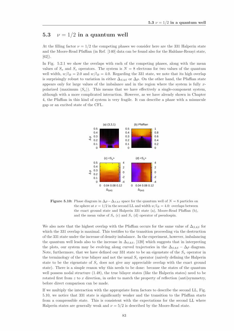
5.3 ν = 1/2 in a quantum well
5.3 ν = 1/2 in a quantum well
At the filling factor ν = 1/2 the competing phases we consider here are the 331 Halperin state
and the Moore-Read Pfaffian (in Ref. [140] data can be found also for the Haldane-Rezayi state,
[62]).
In Fig. 5.2.1 we show the overlaps with each of the competing phases, along with the mean
values of Sx and Sz operators. The system is N = 8 electrons for two values of the quantum
well width, w/lB = 2.0 and w/lB = 4.0. Regarding the 331 state, we note that its high overlap
is surprisingly robust to variation in either ∆SAS or ∆ρ. On the other hand, the Pfaffian state
appears only for large values of the imbalance and in the region where the system is fully x-
polarized (maximum 〈Sx〉). This means that we have effectively a single-component system,
although with a more complicated interaction. However, as we have already shown in Chapter
4, the Pfaffian in this kind of system is very fragile. It can describe a phase with a minuscule
gap or an excited state of the CFL.
(a) (3,3,1)
0 0.1 0.2 0.3 0.4 0.5
∆ ρ
0 0.2 0.4 0.6 0.8 1
(b) Pfaffian
0 0.1 0.2 0.3 0.4 0.5
-4
-2
0
2
4
(c) <Sx>
0 0.04 0.08 0.12∆SAS
0 0.1 0.2 0.3 0.4 0.5
∆ ρ
-4
-2
0
2
4
(d) <Sz>
0 0.04 0.08 0.12∆SAS
Figure 5.10: Phase diagram in ∆ρ−∆SAS space for the quantum well of N = 8 particles on
the sphere at ν = 1/2 in the second LL and width w/lB = 4.0: overlaps between
the exact ground state and Halperin 331 state (a), Moore-Read Pfaffian (b),
and the mean value of Sx (c) and Sz (d) operator of pseudospin.
We also note that the highest overlap with the Pfaffian occurs for the same value of ∆SAS for
which the 331 overlap is maximal. This testifies to the transition proceeding via the destruction
of the 331 state under the increase of density imbalance. In the experiment, however, imbalancing
the quantum well leads also to the increase in ∆SAS , [120] which suggests that in interpreting
the plots, our system may be evolving along curved trajectories in the ∆SAS − ∆ρ diagram.
Note, furthermore, that we have defined our 331 state to be an eigenstate of the Sx operator in
the terminology of the true bilayer and not the usual Sz operator (naively defining the Halperin
state to be the eigenstate of Sz does not give any appreciable overlap with the exact ground
state). There is a simple reason why this needs to be done: because the states of the quantum
well possess nodal structure (1.48), the true bilayer states (like the Halperin states) need to be
rotated first from z to x direction, in order to match the property of reflection (anti)symmetry,
before direct comparison can be made.
If we multiply the interaction with the appropriate form factors to describe the second LL, Fig.
5.10, we notice that 331 state is significantly weaker and the transition to the Pfaffian starts
from a compressible state. This is consistent with the expectations for the second LL where
Halperin states are generally weak and ν = 5/2 is described by the Moore-Read state.
83
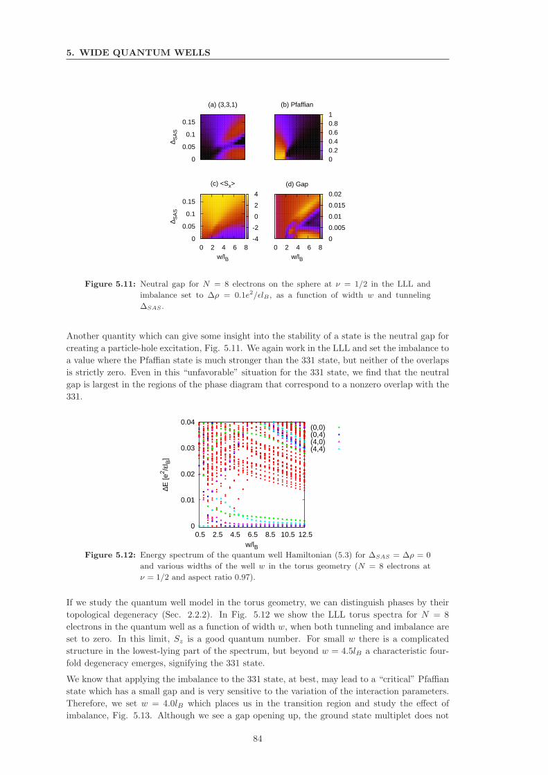
5. WIDE QUANTUM WELLS
(a) (3,3,1)
0
0.05
0.1
0.15
∆ SA
S
0 0.2 0.4 0.6 0.8 1
(b) Pfaffian
-4
-2
0
2
4
(c) <Sx>
0 2 4 6 8w/lB
0
0.05
0.1
0.15
∆ SA
S
0
0.005
0.01
0.015
0.02
(d) Gap
0 2 4 6 8w/lB
Figure 5.11: Neutral gap for N = 8 electrons on the sphere at ν = 1/2 in the LLL and
imbalance set to ∆ρ = 0.1e2/ǫlB , as a function of width w and tunneling
∆SAS .
Another quantity which can give some insight into the stability of a state is the neutral gap for
creating a particle-hole excitation, Fig. 5.11. We again work in the LLL and set the imbalance to
a value where the Pfaffian state is much stronger than the 331 state, but neither of the overlaps
is strictly zero. Even in this “unfavorable” situation for the 331 state, we find that the neutral
gap is largest in the regions of the phase diagram that correspond to a nonzero overlap with the
331.
0
0.01
0.02
0.03
0.04
0.5 2.5 4.5 6.5 8.5 10.5 12.5
∆E [e
2 /εl B
]
w/lB
(0,0)(0,4)(4,0)(4,4)
Figure 5.12: Energy spectrum of the quantum well Hamiltonian (5.3) for ∆SAS = ∆ρ = 0
and various widths of the well w in the torus geometry (N = 8 electrons at
ν = 1/2 and aspect ratio 0.97).
If we study the quantum well model in the torus geometry, we can distinguish phases by their
topological degeneracy (Sec. 2.2.2). In Fig. 5.12 we show the LLL torus spectra for N = 8
electrons in the quantum well as a function of width w, when both tunneling and imbalance are
set to zero. In this limit, Sz is a good quantum number. For small w there is a complicated
structure in the lowest-lying part of the spectrum, but beyond w = 4.5lB a characteristic four-
fold degeneracy emerges, signifying the 331 state.
We know that applying the imbalance to the 331 state, at best, may lead to a “critical” Pfaffian
state which has a small gap and is very sensitive to the variation of the interaction parameters.
Therefore, we set w = 4.0lB which places us in the transition region and study the effect of
imbalance, Fig. 5.13. Although we see a gap opening up, the ground state multiplet does not
84
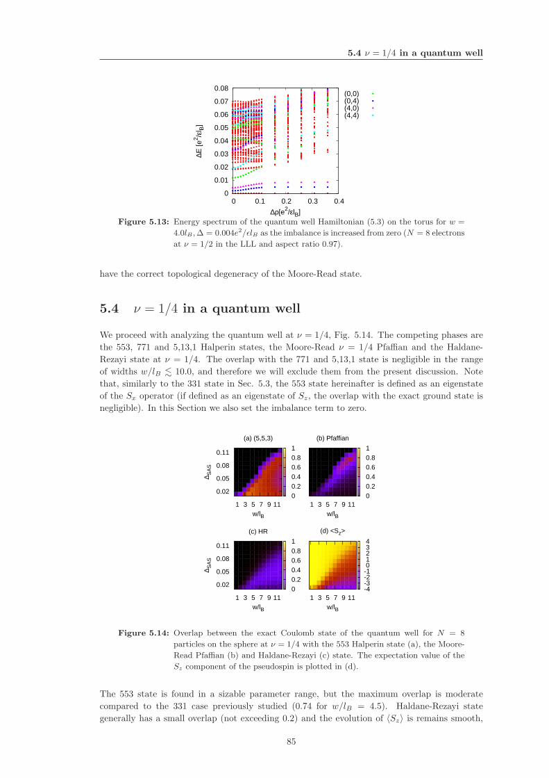
5.4 ν = 1/4 in a quantum well
0
0.01
0.02
0.03
0.04
0.05
0.06
0.07
0.08
0 0.1 0.2 0.3 0.4∆E
[e2 /ε
l B]
∆ρ[e2/εlB]
(0,0)(0,4)(4,0)(4,4)
Figure 5.13: Energy spectrum of the quantum well Hamiltonian (5.3) on the torus for w =
4.0lB , ∆ = 0.004e2/ǫlB as the imbalance is increased from zero (N = 8 electrons
at ν = 1/2 in the LLL and aspect ratio 0.97).
have the correct topological degeneracy of the Moore-Read state.
5.4 ν = 1/4 in a quantum well
We proceed with analyzing the quantum well at ν = 1/4, Fig. 5.14. The competing phases are
the 553, 771 and 5,13,1 Halperin states, the Moore-Read ν = 1/4 Pfaffian and the Haldane-
Rezayi state at ν = 1/4. The overlap with the 771 and 5,13,1 state is negligible in the range
of widths w/lB . 10.0, and therefore we will exclude them from the present discussion. Note
that, similarly to the 331 state in Sec. 5.3, the 553 state hereinafter is defined as an eigenstate
of the Sx operator (if defined as an eigenstate of Sz, the overlap with the exact ground state is
negligible). In this Section we also set the imbalance term to zero.
0 0.2 0.4 0.6 0.8 1
(a) (5,5,3)
1 3 5 7 9 11w/lB
0.02
0.05
0.08
0.11
∆ SA
S
0 0.2 0.4 0.6 0.8 1
(b) Pfaffian
1 3 5 7 9 11w/lB
0 0.2 0.4 0.6 0.8 1
(c) HR
1 3 5 7 9 11w/lB
0.02
0.05
0.08
0.11
∆ SA
S
-4-3-2-1 0 1 2 3 4
(d) <Sz>
1 3 5 7 9 11w/lB
Figure 5.14: Overlap between the exact Coulomb state of the quantum well for N = 8
particles on the sphere at ν = 1/4 with the 553 Halperin state (a), the Moore-
Read Pfaffian (b) and Haldane-Rezayi (c) state. The expectation value of the
Sz component of the pseudospin is plotted in (d).
The 553 state is found in a sizable parameter range, but the maximum overlap is moderate
compared to the 331 case previously studied (0.74 for w/lB = 4.5). Haldane-Rezayi state
generally has a small overlap (not exceeding 0.2) and the evolution of 〈Sz〉 is remains smooth,
85
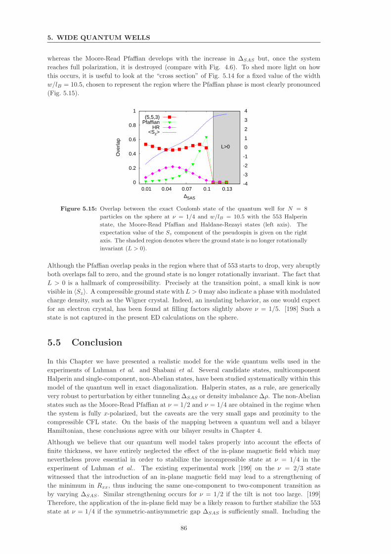
5. WIDE QUANTUM WELLS
whereas the Moore-Read Pfaffian develops with the increase in ∆SAS but, once the system
reaches full polarization, it is destroyed (compare with Fig. 4.6). To shed more light on how
this occurs, it is useful to look at the “cross section” of Fig. 5.14 for a fixed value of the width
w/lB = 10.5, chosen to represent the region where the Pfaffian phase is most clearly pronounced
(Fig. 5.15).
0
0.2
0.4
0.6
0.8
1
0.01 0.04 0.07 0.1 0.13-4
-3
-2
-1
0
1
2
3
4O
verla
p
∆SAS
L>0
(5,5,3)Pfaffian
HR<Sz>
Figure 5.15: Overlap between the exact Coulomb state of the quantum well for N = 8
particles on the sphere at ν = 1/4 and w/lB = 10.5 with the 553 Halperin
state, the Moore-Read Pfaffian and Haldane-Rezayi states (left axis). The
expectation value of the Sz component of the pseudospin is given on the right
axis. The shaded region denotes where the ground state is no longer rotationally
invariant (L > 0).
Although the Pfaffian overlap peaks in the region where that of 553 starts to drop, very abruptly
both overlaps fall to zero, and the ground state is no longer rotationally invariant. The fact that
L > 0 is a hallmark of compressibility. Precisely at the transition point, a small kink is now
visible in 〈Sz〉. A compressible ground state with L > 0 may also indicate a phase with modulated
charge density, such as the Wigner crystal. Indeed, an insulating behavior, as one would expect
for an electron crystal, has been found at filling factors slightly above ν = 1/5. [198] Such a
state is not captured in the present ED calculations on the sphere.
5.5 Conclusion
In this Chapter we have presented a realistic model for the wide quantum wells used in the
experiments of Luhman et al. and Shabani et al. Several candidate states, multicomponent
Halperin and single-component, non-Abelian states, have been studied systematically within this
model of the quantum well in exact diagonalization. Halperin states, as a rule, are generically
very robust to perturbation by either tunneling ∆SAS or density imbalance ∆ρ. The non-Abelian
states such as the Moore-Read Pfaffian at ν = 1/2 and ν = 1/4 are obtained in the regime when
the system is fully x-polarized, but the caveats are the very small gaps and proximity to the
compressible CFL state. On the basis of the mapping between a quantum well and a bilayer
Hamiltonian, these conclusions agree with our bilayer results in Chapter 4.
Although we believe that our quantum well model takes properly into account the effects of
finite thickness, we have entirely neglected the effect of the in-plane magnetic field which may
nevertheless prove essential in order to stabilize the incompressible state at ν = 1/4 in the
experiment of Luhman et al.. The existing experimental work [199] on the ν = 2/3 state
witnessed that the introduction of an in-plane magnetic field may lead to a strengthening of
the minimum in Rxx, thus inducing the same one-component to two-component transition as
by varying ∆SAS . Similar strengthening occurs for ν = 1/2 if the tilt is not too large. [199]
Therefore, the application of the in-plane field may be a likely reason to further stabilize the 553
state at ν = 1/4 if the symmetric-antisymmetric gap ∆SAS is sufficiently small. Including the
86
5.5 Conclusion
effect of an in-plane field is a rather complicated problem, even in the simpler models, because
the motion along z-axis is no longer separable from the in-plane motion. Another possibility is
that ν = 1/2 state in the wide quantum well is an imbalanced two-component CF state, [122]
however there is no such simple candidate for ν = 1/4.
In order to answer without ambiguity which of the possibilities is actually realized in the quantum
well under the experimental conditions of Refs. [118, 119], it would be useful to know the
dependence of the activation gap as a function of ∆SAS and also as a function of transferred
charge from the front to the back of the quantum well using a gate biasing. These results would
help to discriminate between the one-component and two-component nature of the ground state.
87
5. WIDE QUANTUM WELLS
88
Chapter 6
Graphene as a multicomponent
FQH system
This Chapter explores interacting states in graphene in a strong magnetic field. Due to the
valley and spin degrees of freedom, graphene can be described by an internal SU(4) symmetry.
We analyze how the four-component structure of graphene may have particular signatures in
possible FQHEs. We introduce the interaction model for electrons restricted to a single graphene
LL (Sec. 6.1) and concentrate on the spin-valley SU(4) symmetric part of the interaction model,
which constitutes the leading energy scale. In Section 6.2 we investigate via the pseudopotential
method the possible FQH states in graphene in the LLs n = 0 and 1. Recent reviews [200, 201]
contain many details on the interaction model for graphene and expectations for a FQHE, as
well as the original papers [200] and [202] that this Chapter is based on.
6.1 Interaction model for graphene in a strong magnetic
field
From a theoretical point of view, long-range interactions in graphene are expected to be relevant.
Let us look at the dimensionless ratio rs of the characteristic Coulomb energy EC and the kinetic
energy Ekin:
rs =EC
Ekin=
e2/ǫl
~vF kF≈ 2.2
ǫ, (6.1)
where we substituted EC = e2/ǫl (l being the average inter-electronic distance and ǫ the dielectric
constant of the graphene sheet environment) and Ekin = ~vF kF ∼ ~vF /l, vF being the Fermi
velocity. Therefore, the ratio rs places graphene in an intermediate range of correlation strengths
(large values of rs would signal strong coupling). Notice in (6.1) that a convenient way to vary
the correlation strength in graphene is via adjustment of the dielectric constant of the substrate.
Additionally, we can estimate the Thomas-Fermi wave vector kGTF which defines the characteristic
length λTF ∼ 1/kGTF above which the Coulomb interaction potential is screened:
kGTF ∼ rskF ∼
√nel, (6.2)
which vanishes at the Dirac points where the carrier density nel goes to zero. Therefore, the
screening length is very large in graphene and one has to treat the long-range Coulomb interaction
directly, instead of attempting to use a Hubbard-like model.
In order to quantify the degree of separation between the energy scales in graphene in the
magnetic field, one needs to compare the typical energy for exchange interaction
VC = e2/ǫRC ≃ 25√
B[T]/ǫ√
2n+ 1 meV,
89
6. GRAPHENE AS A MULTICOMPONENT FQH SYSTEM
in terms of the cyclotron radius RC = lB√
2n+ 1, with the magnetic length lB =√
~/eB =
25/√
B[T] nm, to the LL separation
∆n =√
2~(vF /lB)(√n+ 1−
√n).
In spite of the decreasing LL separation in the large-n limit, the ratio between both energy scales
remains constant and reproduces the fine-structure constant of graphene,
αG = VC/∆n = e2/~vF ǫ ≃ 2.2/ǫ.
Notice that the Coulomb interaction respects the fourfold spin-valley degeneracy to lowest order
in a/lB ≃ 0.005√
B[T], where a = 0.14 nm is the distance between nearest-neighbour carbon
atoms in graphene. [201] This fourfold spin-valley symmetry is described in the framework of the
SU(4) group which covers the two copies of the SU(2) spin and the SU(2) valley isospin. Lattice
effects break this SU(4) symmetry at an energy scale VC(a/lB) ≃ 0.1B[T]/ǫ meV [203, 204, 205,
206], which is roughly on the same order of magnitude as the expected Zeeman effect in graphene
[207]. Other symmetry-breaking mechanisms have been proposed [208, 209, 210, 211] but happen
to be equally suppressed with respect to the leading interaction energy scale VC . An exception
may be graphene on a graphite substrate, where the natural lattice commensurability of the
substrate and the sample may lead to a stronger coupling than for graphene on a SiO2 substrate
[212]. This yields a mass term in the Dirac Hamiltonian which lifts the valley degeneracy of the
zero-energy LL [208].
Based on these considerations, graphene in a strong magnetic field may thus be viewed as a
four-component quantum Hall system. An interesting theoretical expectation resulting from
this feature is the formation of a quantum Hall ferromagnet at ν = ±1 [203, 204, 213, 214] with
SU(4)-skyrmion excitations, which may have peculiar magnetic properties [214, 215]. Also for
the FQHE, the SU(4) spin-valley symmetry is expected to play a relevant role and has been
considered within a CF approach [216] as well as one based on SU(4) Halperin wave functions
[87, 126].
In the case of a partially filled LL, we can use the Hamiltonian we defined in (1.19), describing
only intra-LL excitations, where the Fourier components ρλn(q) of the density operator are
constructed solely from states within the n-th LL in the band λ (λ = + for the conduction and
λ = − for the valence band). This construction is analogous to that used in the conventional
2DEG, but the density operators ρn(q) are now built up from spinor states of the 2D Dirac
equation,
ψξλn,m =
1√2
(
|n− 1,m〉λ|n,m〉
)
(6.3)
for n 6= 0 and
ψξn=0,m =
(
0
|n = 0,m〉
)
(6.4)
for the zero-energy LL n = 0, in terms of the harmonic oscillator states |n,m〉 and the guiding-
center quantum number m = 0. Here, we have chosen the first component of the spinor to
represent at the K point (ξ = +) the amplitude on the A sublattice and that on the B sublattice
at the K ′ point (ξ = −). Notice that the valley and the sublattice indices happen to be the same
in the zero-energy LL n = 0 and that, thus, a perturbation that breaks the inversion symmetry
(the equivalence of the two sublattices) automatically lifts the valley degeneracy [208, 209, 210,
211]. In terms of the spinor states (6.3) and (6.4), the density operator may be written
ρλn(q) =∑
ξ,m
(
ψξλn,m
)†e−iq·rψξ
λn,m′c†λn,m;ξcλn,m′;ξ , (6.5)
where c(†)λn,m;ξ annihilates (creates) an electron in the state ψξ
λn,m. In Eq. (6.5), we have neglected
the contributions that are off-diagonal in the valley index. Indeed, these contributions give rise
90
6.1 Interaction model for graphene in a strong magnetic field
to a rapidly oscillating phase exp(±iK · r) in the matrix elements, where ±K = ±(4π/3√
3a)ex
is the location of the K and K ′ points, respectively, and yield terms in the Hamiltonian (1.19),
which break the valley-SU(2) symmetry of the interaction. They are suppressed by a factor a/lBwith respect to the leading interaction energy scale e2/ǫlB [203] and, for the sake of simplicity
and because of their smallness, we neglect these terms here.
Within the symmetric gauge, A = (B/2)(−y, x, 0), the position operator r in Eq. (6.5) may be
decomposed into the guiding-center position R and the cyclotron variable η. Whereas the latter
only affects the quantum number n, R acts on m, and we may therefore rewrite the density
operator (6.5), ρλn(q) = Fn(q)ρ(q), as a product of the projected density operator
ρ(q) =∑
ξ;m,m′
⟨
m∣
∣e−iq·R∣∣m′⟩ c†λn,m;ξcλn,m′;ξ (6.6)
and the graphene form factor
Fn(q) =1
2
(⟨
n− 1∣
∣e−iq·η∣∣n− 1
⟩
+⟨
n∣
∣e−iq·η∣∣n⟩)
=1
2
[
Ln−1
(
q2
2
)
+ Ln
(
q2
2
)]
e−q2/4
(6.7)
for n 6= 0, in terms of Laguerre polynomials, and
Fn=0(q) =⟨
0∣
∣e−iq·η∣∣ 0⟩
= e−q2/4 (6.8)
for n = 0. With the help of the projected density operators, the interaction Hamiltonian (1.19)
reads
Hλn =1
2
∑
q
vGn (q)ρ(−q)ρ(q), (6.9)
where we have defined the effective interaction potential for graphene LLs,
vGn (q) =
2πe2
ǫq[Fn(q)]
2. (6.10)
Notice that the structure of the Hamiltonian (6.9) is that of electrons in a conventional 2DEG
restricted to a single LL if one notices that the projected density operators satisfy the magnetic
translation algebra [45]
[ρ(q), ρ(q′)] = 2i sin
(
q′ ∧ q
2
)
ρ(q + q′), (6.11)
where q′ ∧ q ≡ q′xqy − qxq′y is the 2D vector product. This is a remarkable result in view of
the different translation symmetries of the zero-field Hamiltonian; whereas the electrons in the
2DEG are non-relativistic and therefore satisfy Galilean invariance, the relativistic electrons
in graphene are Lorentz-invariant. However, once submitted to a strong magnetic field and
restricted to a single LL, the translation symmetry of the electrons is described by the magnetic
translation group in both cases.
6.1.1 SU(4) symmetry
The most salient difference between the conventional 2DEG and graphene arises from the larger
internal symmetry of the latter, due to its valley degeneracy. This valley degeneracy may be
accounted for by an SU(2) valley isospin in addition to the physical SU(2) spin, which we
have omitted so far and the symmetry of which is respected by the interaction Hamiltonian.
91
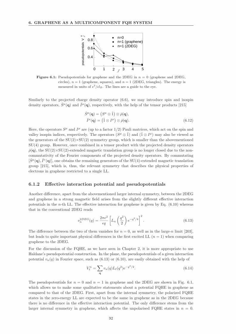
6. GRAPHENE AS A MULTICOMPONENT FQH SYSTEM
1 2 3 4 5 6
0.4
0.6
0.8
nps
eudo
pote
ntia
ls V
n=1 (2DEG)n=1 (graphene)n=0
0 1 2 3 4 5
0.8
0.6
0.4
Figure 6.1: Pseudopotentials for graphene and the 2DEG in n = 0 (graphene and 2DEG,
circles), n = 1 (graphene, squares), and n = 1 (2DEG, triangles). The energy is
measured in units of e2/ǫlB . The lines are a guide to the eye.
Similarly to the projected charge density operator (6.6), we may introduce spin and isospin
density operators, Sµ(q) and Iµ(q), respectively, with the help of the tensor products [215]
Sµ(q) =(
Sµ ⊗ 1)
⊗ ρ(q),
Iµ(q) =(
1⊗ Iµ)
⊗ ρ(q). (6.12)
Here, the operators Sµ and Iµ are (up to a factor 1/2) Pauli matrices, which act on the spin and
valley isospin indices, respectively. The operators (Sµ ⊗ 1) and (1⊗ Iµ) may also be viewed as
the generators of the SU(2)×SU(2) symmetry group, which is smaller than the abovementioned
SU(4) group. However, once combined in a tensor product with the projected density operators
ρ(q), the SU(2)×SU(2)-extended magnetic translation group is no longer closed due to the non-
commutativity of the Fourier components of the projected density operators. By commutating
[Sµ(q), Iν(q)], one obtains the remaining generators of the SU(4)-extended magnetic translation
group [215], which is, thus, the relevant symmetry that describes the physical properties of
electrons in graphene restricted to a single LL.
6.1.2 Effective interaction potential and pseudopotentials
Another difference, apart from the abovementioned larger internal symmetry, between the 2DEG
and graphene in a strong magnetic field arises from the slightly different effective interaction
potentials in the n-th LL. The effective interaction for graphene is given by Eq. (6.10) whereas
that in the conventional 2DEG reads
v2DEGn (q) =
2πe2
ǫq
[
Ln
(
q2
2
)
e−q2/4
]2
. (6.13)
The difference between the two of them vanishes for n = 0, as well as in the large-n limit [203],
but leads to quite important physical differences in the first excited LL (n = 1) when comparing
graphene to the 2DEG.
For the discussion of the FQHE, as we have seen in Chapter 2, it is more appropriate to use
Haldane’s pseudopotential construction. In the plane, the pseudopotentials of a given interaction
potential vn(q) in Fourier space, such as (6.13) or (6.10), are easily obtained with the help of
V nℓ =
∑
q
vn(q)Lℓ(q2)e−q2/2. (6.14)
The pseudopotentials for n = 0 and n = 1 in graphene and the 2DEG are shown in Fig. 6.1,
which allows us to make some qualitative statements about a potential FQHE in graphene as
compared to that of the 2DEG. First, apart from the internal symmetry, the polarized FQHE
states in the zero-energy LL are expected to be the same in graphene as in the 2DEG because
there is no difference in the effective interaction potential. The only difference stems from the
larger internal symmetry in graphene, which affects the unpolarised FQHE states in n = 0.
92
6.2 Multicomponent trial wave functions for graphene
Second, the n = 1 LL in graphene is much more reminiscent of the n = 0 LL than of the n = 1
LL in the 2DEG. From an interaction point of view, one would therefore expect that the quantum
phases encountered in the n = 1 graphene LL are merely a copy of those in n = 0. Furthermore,
if one considers spin-polarised FQHE states, only pseudopotentials with odd angular momentum
are relevant due to the fermionic nature of the electrons. It is apparent from Fig. 6.1 that odd-ℓ
pseudopotentials are systematically larger in n = 1 than in n = 0. Therefore, the overall energy
scale of FQHE states in n = 1 is slightly larger (by ∼ 10%) than in n = 0, and one would expect,
somewhat counterintuitively, that the n = 1 FQHE states are more stable than those in n = 0,
for the same B-field value. These qualitative predictions [203] have been corroborated within
ED studies, where only the valley isospin degree of freedom was considered and the physical spin
was taken as completely polarized [217, 218].
6.2 Multicomponent trial wave functions for graphene
In the following, we consider some particular subclasses of the trial wave functions (1.47), which
are natural candidates for a FQHE in graphene. Explicitely, we label the four spin-valley com-
ponents as 1 = (↑,K), 2 = (↑,K ′), 3 = (↓,K), and 4 = (↓,K ′), where the first component
denotes the spin orientation (↑ or ↓) and the second the valley (K or K ′). We investigate wave
functions, where all intracomponent exponents are identical mi = m, i.e. we consider the same
interaction potential for any of the components, as it is the case in graphene. Furthermore, we
consider n13 = n24 ≡ na and n12 = n14 = n23 = n34 ≡ ne, which makes an explicit distinction
between inter-component correlations in the same valley (na) and those in different valleys (ne).
This distinction may occur somewhat arbitrary – indeed, it does no longer treat the spin on the
same footing as the valley isospin – but it happens to be useful in some cases if one intends to
describe states with intermediate polarization, such as for a moderate Zeeman field. The equiv-
alence between spin and valley isospin is naturally restored for ne = na. We use the notation
[m;ne, na] to describe these subclasses of trial wave functions (1.47), the validity of which we
check by ED of N particles on a sphere [42].
6.2.1 [m; m,m] wave functions
If all exponents are identical odd integers m, we obtain a completely antisymmetric orbital
wave function, which is nothing other than the Laughlin wave function (1.20). In this case, the
distinction between the components vanishes, and the component filling factors are not fixed –
one may, without changing the orbital wave function, fill only one particular component as well
as another or distribute the particles over all components. Only the total filling factor is fixed
at ν = 1/m. The corresponding exponent matrix M (1.56) is indeed not invertible (of rank 1),
and the residual freedom of distributing the electrons over the four components may be viewed
as the arbitrary orientation of a four-spinor in SU(4) space. The Laughlin wave function in
graphene is therefore associated with an SU(4) ferromagnetism, similar to that of the state at
νG = ±1 [203, 204, 213, 214, 215], where a graphene quantum Hall effect has been observed at
high magnetic fields [207].
As already mentioned above, the Laughlin wave function has the good property of screening all
pseudopotentials with angular momentum ℓ < m and has, for m = 3, the usual large overlap
with the Coulomb ground state [216]. However, states described by the [m;m,m] wave function
are ground-state candidates for the filling factors ν = 1/m, which correspond to the graphene
filling factors (see Eq. 1.57) νG = −2+1/m or hole states at νG = 2−1/m. These filling factors
do not correspond to the FQHE at νG = ±1/3 observed in the experiments [124, 125].
93
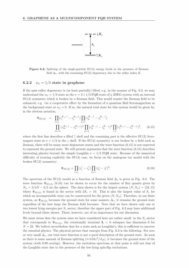
6. GRAPHENE AS A MULTICOMPONENT FQH SYSTEM
Figure 6.2: Splitting of the single-particle SU(4) energy levels in the presence of Zeeman
field ∆z, with the remaining SU(2) degeneracy due to the valley index K.
6.2.2 νG = 1/3 state in graphene
If the spin-valley degeneracy is (at least partially) lifted, e.g. in the manner of Fig. 6.2, we may
understand the νG = 1/3 state as the ν = 2+1/3 FQH state of a 2DEG system with an internal
SU(4) symmetry which is broken by a Zeeman field. This would require the Zeeman field to be
enhanced, e.g. via a cooperative effect by the formation of a quantum Hall ferromagnetism as
the background state at νG = 0. If so, the natural trial state for this system would be given by,
in the obvious notation,
ΨSU(4) =∏
i<j
(zK+,↑i − zK+,↑
j )∏
k<l
(zK−,↑k − zK−,↑
l )
∏
m<n
(zK+,↓m − zK+,↓
n )3∏
p<q
(zK−,↓p − zK−,↓
q )3∏
r,s
(zK+,↓r − zK−,↓
s )3, (6.15)
where the first line describes a filled ↑ shell and the remaining part is the effective SU(2) ferro-
magnet state at ν = 1/3 in the ↓ shell. If the SU(4) symmetry is not broken by a field such as
Zeeman, there will be many more degenerate states and the wave function (6.15) is not expected
to represent the ground state. We will present arguments that the wave function (6.15) describes
interesting physics beyond the simple Laughlin ν = 1/3 FQH state. Because of the numerical
difficulty of treating explicitly the SU(4) case, we focus on the analogous toy model with the
broken SU(2) symmetry:
ΨSU(2) =∏
i<j
(z↑i − z↑j )∏
k<l
(z↓k − z↓l )3. (6.16)
The spectrum of the SU(2) model as a function of Zeeman field ∆z is given in Fig. 6.3. The
wave function ΨSU(2) (6.16) can be shown to occur for the number of flux quanta given by
Nφ = 3/4N − 3/2 on the sphere. The data shown is for the largest system (N,Nφ) = (22, 15)
where ΨSU(2) is found in the sector with 2Sz = 10. This is also the largest value of Sz for
which an incompressible state can be constructed for the given (N,Nφ). Therefore, in our finite
system, as ΨSU(2) becomes the ground state for some nonzero ∆z, it remains the ground state
regardless of the how large the Zeeman field becomes. Note that we have shown only one or
two lowest lying energies per Sz sector, therefore the upper part of Fig. 6.3 may have additional
levels beyond those shown. These, however, are of no importance for our discussion.
We must stress that the system sizes we have considered here are rather small: in the Sz sector
that corresponds to ΨSU(2), the rotationally invariant L = 0 subspace has dimension 6 for
N = 22. We believe nevertheless that for a state such as Laughlin’s, this is sufficient to uncover
the essential physics. The physical picture that emerges from Fig. 6.3 is the following. For zero
or very small ∆z, our trial wave function is not a good description of the ground state. As soon
as there is some amount of Zeeman splitting (≈ 0.01e2/ǫlB), it becomes the ground state of the
system (with 0.99 overlap). However, the excitation spectrum at that point is still not that of
the Laughlin state due to the presence of the low-lying spin-flip excitations.
94
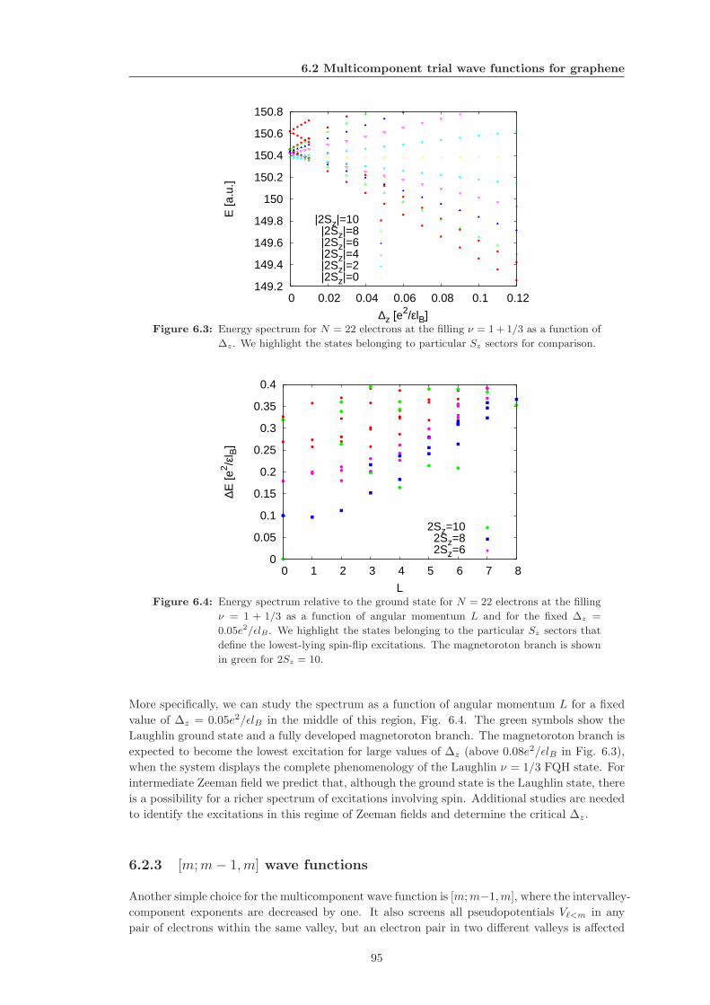
6.2 Multicomponent trial wave functions for graphene
149.2
149.4
149.6
149.8
150
150.2
150.4
150.6
150.8
0 0.02 0.04 0.06 0.08 0.1 0.12
E [a
.u.]
∆z [e2/εlB]
|2Sz|=10|2Sz|=8|2Sz|=6|2Sz|=4|2Sz|=2|2Sz|=0
Figure 6.3: Energy spectrum for N = 22 electrons at the filling ν = 1 + 1/3 as a function of
∆z. We highlight the states belonging to particular Sz sectors for comparison.
0
0.05
0.1
0.15
0.2
0.25
0.3
0.35
0.4
0 1 2 3 4 5 6 7 8
∆E [e
2 /εl B
]
L
2Sz=102Sz=82Sz=6
Figure 6.4: Energy spectrum relative to the ground state for N = 22 electrons at the filling
ν = 1 + 1/3 as a function of angular momentum L and for the fixed ∆z =
0.05e2/ǫlB . We highlight the states belonging to the particular Sz sectors that
define the lowest-lying spin-flip excitations. The magnetoroton branch is shown
in green for 2Sz = 10.
More specifically, we can study the spectrum as a function of angular momentum L for a fixed
value of ∆z = 0.05e2/ǫlB in the middle of this region, Fig. 6.4. The green symbols show the
Laughlin ground state and a fully developed magnetoroton branch. The magnetoroton branch is
expected to become the lowest excitation for large values of ∆z (above 0.08e2/ǫlB in Fig. 6.3),
when the system displays the complete phenomenology of the Laughlin ν = 1/3 FQH state. For
intermediate Zeeman field we predict that, although the ground state is the Laughlin state, there
is a possibility for a richer spectrum of excitations involving spin. Additional studies are needed
to identify the excitations in this regime of Zeeman fields and determine the critical ∆z.
6.2.3 [m; m− 1,m] wave functions
Another simple choice for the multicomponent wave function is [m;m−1,m], where the intervalley-
component exponents are decreased by one. It also screens all pseudopotentials Vℓ<m in any
pair of electrons within the same valley, but an electron pair in two different valleys is affected
95
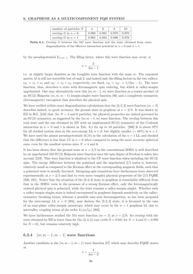
6. GRAPHENE AS A MULTICOMPONENT FQH SYSTEM
number of particles N 4 6 8 10
overlap O in n = 0 0.990 0.985 0.979 0.970
overlap O in n = 1 0.965 0.882 0.896 0.876
Table 6.1: Overlap O between the 332 wave function and the state obtained from exact
diagonalization of the effective interaction potential in n = 0 and n = 1.
by the pseudopotential Vℓ=m−1. The filling factor, where this wave function may occur, is
ν =2
2m− 1,
i.e. at slightly larger densities as the Laughlin wave function with the same m. The exponent
matrix M is still not invertible but of rank 2, and indeed only the filling factors in the two valleys,
νK = ν1 + ν3 and νK′ = ν2 + ν4, respectively, are fixed, νK = νK′ = 1/(2m − 1). The wave
function, thus, describes a state with ferromagnetic spin ordering, but which is valley-isospin
unpolarized. One may alternatively view this [m;m−1,m] wave function as a tensor product of
an SU(2) Halperin (m,m,m− 1) isospin-singlet wave function [86] and a completely symmetric
(ferromagnetic) two-spinor that describes the physical spin.
We have verified within exact diagonalization calculations that the [3; 2, 3] wave function (m = 3)
describes indeed, to great accuracy, the ground state in graphene at ν = 2/5. It was shown by
ED in Ref. [216] that, for N = 4 and 6 particles, the physical properties are indeed governed by
an SU(2) symmetry, as suggested by the [m;m− 1,m] wave function. The overlap between this
trial state and the one obtained by ED with an implemented SU(2) symmetry of the Coulomb
interaction in n = 0 and 1 is shown in Tab. 6.1 for up to 10 particles. [200] It is above 97%
for all studied system sizes in the zero-energy LL n = 0, but slightly smaller (∼ 88%) in n = 1.
We have used the planar pseudopotentials (6.14) in the calculation of the n = 1 LL and checked
that the difference is less than 1% in n = 0 when compared to using the more accurate spherical
ones, even for the smallest system sizes N = 4 and 6.
It has been shown that the ground state at ν = 2/5 in the conventional 2DEG is well described
by an unpolarized 332 SU(2) Halperin wave function once the spin degree of freedom is taken into
account [219]. This wave function is identical to the CF wave function when including the SU(2)
spin. The energy difference between the polarized and the unpolarized 2/5 states is, however,
relatively small as compared to the Zeeman effect at the corresponding magnetic fields, such that
a polarized state is usually favoured. Intriguing spin transitions have furthermore been observed
experimentally at ν = 2/5 and hint to even more complex physical properties of the 2/5 FQHE
[220, 221]. Notice that the situation of the [3; 2, 3] state in graphene is remarkably different from
that in the 2DEG: even in the presence of a strong Zeeman effect, only the ferromagnetically
ordered physical spin is polarized, while the state remains a valley-isospin singlet. Whether such
a valley-isospin singlet state is indeed encountered in graphene depends sensitively on the valley-
symmetry breaking terms; whereas a possible easy-axis ferromagnetism, as has been proposed
for the zero-energy LL n = 0 [204], may destroy the [3; 2, 3] state, it is favoured in the case
of an easy-plane valley-isospin anisotropy, which may occur in the n = 1 graphene LL due to
intervalley coupling terms of the order VC(a/lB) [203].
We have furthermore studied the 554 wave function (m = 5) at ν = 2/9. Its overlap with the
state obtained by ED is lower than for the (3, 3, 2) case (with O = 0.941 for N = 4 and O = 0.892
for N = 6), but remains relatively high.
6.2.4 [m; m− 1,m− 1] wave functions
Another candidate is the [m;m− 1,m− 1] wave function [87] which may describe FQHE states
at
ν =4
4m− 3.
96
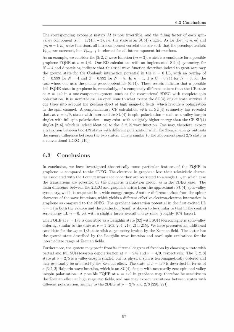
6.3 Conclusions
The corresponding exponent matrix M is now invertible, and the filling factor of each spin-
valley component is ν = 1/(4m− 3), i.e. the state is an SU(4) singlet. As for the [m;m,m] and
[m;m−1,m] wave functions, all intracomponent correlations are such that the pseudopotentials
Vℓ<m are screened, but Vℓ=m−1 is relevant for all intercomponent interactions.
As an example, we consider the [3; 2, 2] wave function (m = 3), which is a candidate for a possible
graphene FQHE at ν = 4/9. Our ED calculations with an implemented SU(4) symmetry, for
N = 4 and 8 particles, indicate that this trial wave function describes indeed to great accuracy
the ground state for the Coulomb interaction potential in the n = 0 LL, with an overlap of
O = 0.999 for N = 4 and O = 0.992 for N = 8. In n = 1, it is O = 0.944 for N = 8, for the
case where one uses the planar pseudopotentials (6.14). These results indicate that a possible
4/9 FQHE state in graphene is, remarkably, of a completely different nature than the CF state
at ν = 4/9 in a one-component system, such as the conventional 2DEG with complete spin
polarization. It is, nevertheless, an open issue to what extent the SU(4) singlet state survives if
one takes into account the Zeeman effect at high magnetic fields, which favours a polarization
in the spin channel. A complementary CF calculation with an SU(4) symmetry has revealed
that, at ν = 4/9, states with intermediate SU(4) isospin polarization – such as a valley-isospin
singlet with full spin polarization – may exist, with a slightly higher energy than the CF SU(4)
singlet [216], which is indeed identical to the [3; 2, 2] wave function. One may, therefore, expect
a transition between two 4/9 states with different polarization when the Zeeman energy outcasts
the energy difference between the two states. This is similar to the abovementioned 2/5 state in
a conventional 2DEG [219].
6.3 Conclusions
In conclusion, we have investigated theoretically some particular features of the FQHE in
graphene as compared to the 2DEG. The electrons in graphene lose their relativistic charac-
ter associated with the Lorentz invariance once they are restricted to a single LL, in which case
the translations are governed by the magnetic translation group, as in the 2DEG case. The
main difference between the 2DEG and graphene arises from the approximate SU(4) spin-valley
symmetry, which is respected in a wide energy range. Another difference arises from the spinor
character of the wave functions, which yields a different effective electron-electron interaction in
graphene as compared to the 2DEG. The graphene interaction potential in the first excited LL
n = 1 (in both the valence and the conduction band) is shown to be similar to that in the central
zero-energy LL n = 0, yet with a slightly larger overall energy scale (roughly 10% larger).
The FQHE at ν = 1/3 is described as a Laughlin state [32] with SU(4)-ferromagnetic spin-valley
ordering, similar to the state at ν = 1 [203, 204, 213, 214, 215]. We have presented an additional
candidate for the νG = 1/3 state with a symmetry broken by the Zeeman field. The latter has
the ground state described by the Laughlin wave function and novel spin excitations for the
intermediate range of Zeeman fields.
Furthermore, the system may profit from its internal degrees of freedom by choosing a state with
partial and full SU(4)-isospin depolarisation at ν = 2/5 and ν = 4/9, respectively. The [3; 2, 3]
state at ν = 2/5 is a valley-isospin singlet, but its physical spin is ferromagnetically ordered and
may eventually be oriented by the Zeeman effect. The state at ν = 4/9 is described in terms of
a [3; 2, 2] Halperin wave function, which is an SU(4) singlet with necessarily zero spin and valley
isospin polarisation. A possible FQHE at ν = 4/9 in graphene may therefore be sensitive to
the Zeeman effect at high magnetic fields, and one may expect transitions between states with
different polarisation, similar to the 2DEG at ν = 2/5 and 2/3 [220, 221].
97
6. GRAPHENE AS A MULTICOMPONENT FQH SYSTEM
98
Chapter 7
Outlook
In this thesis we have presented studies of a variety of systems where multicomponent degrees
of freedom determine the physics or can be used as a proxy towards more exotic, non-Abelian
phases of matter. The latter remain one of the most exciting theoretical concepts advanced in
condensed matter physics awaiting their experimental confirmation. Such phases include, among
others, the p-wave paired phase in the ν = 1 bilayer, the Pfaffian-like states in the wide quantum
wells or yet unobserved analogues in graphene, which all represent exciting venues for future
studies.
The quantum Hall bilayer at ν = 1 remains the subject of much experimental work. Recent
studies point out to the importance of spin physics in the incompressible-compressible transition
that was entirely neglected in almost all of the theoretical work including our discussion in
Section 3. The question of an intermediate phase between the 111 state and the two Fermi
liquids ,although an unlikely possibility, remains open. Moreover, the new measurements probe
the nature of the critical current in the zero bias anomaly experiments and find that the simple
models of a clean, homogeneous bilayer are insufficient and more work is needed to understand
the fine details of the disordering of the QH bilayer superfluid.
Understanding of the non-Abelian phases of matter in the context of FQHE has significantly
advanced over the last decade, but this knowledge is certainly incomplete because we do not know
what kind of physical interaction favors such phases of matter and how they can be potentially
engineered in real samples. Is there a ν = 5/2 analogue of the Moore-Read state in graphene?
Having a clearer idea of material properties, even outside the usual GaAs structures, that would
favor states such as the Moore-Read Pfaffian should also give a definitive answer as to whether
the even-denominator states in the wide quantum wells in the LLL are non-Abelian or not. The
effect of Landau level mixing which seems to play an important role in the experiment should
also prove interesting to study in more detail. Systems such as graphene bilayers could be useful
to develop a feeling for the magnitude of its effect because graphene bilayer represents a case of
an extreme LL mixing when the zeroth and first excited LL can be brought to coincide.
Finally, there is a fundamental theoretical problem of the role of non-unitary conformal field the-
ories and the wave functions they define as the trial QH states. Can these describe incompressible
QH states and, if not, what is the precise nature of gaplessness of their excitations.
99
7. OUTLOOK
100
Appendix A
DiagHam
Numerical calculations in this thesis have been performed using DiagHam libraries:
http://www.nick-ux.org/diagham/
DiagHam is a set of C++ classes and in-built programs that provide the framework for exact
diagonalization of various quantum models, in particular the fractional quantum Hall effect.
It is subject to the GPL public license and the source code is most easily obtained from the
Subversion repositories:
svn checkout https://www.nick-ux.org/diagham/svn/trunk DiagHam
The minimal installation assumes that internal DiagHam libraries will be used for full diagonal-
ization. In the root of the checked-out source package one needs to execute
./bootstrap.sh
./configure <options>
make
where configure supports various options that can be listed with the switch --help. For FQHE
programs, one has to use --enable-fqhe. In addition, it is possible to use Lapack libraries for
full diagonalization, routines from Gnu Scientific Library (GSL), partial support for MPI etc.
DiagHam has been used for very large-scale diagonalization problems (matrices of the order 108).
Diagonalization of a given quantum lattice model such as the FQHE proceeds by defining (1)
the Hilbert space of the system and (2) the Hamiltonian which acts on the vectors in the given
Hilbert space. The Hilbert space of the FQH system depends on the kind of particles (fermions or
bosons), the geometry (disk, sphere and torus) and the internal symmetry (fully polarized, SU(2),
SU(3), SU(4)). Hamiltonian on the other hand also depends on the kind of interaction (two-
body, three-body etc.). We work in the Fock basis where states |j1, j2, . . . , jNe〉 are understood
as binary forms of integer numbers, which makes it easy to manipulate them. This is referred
to as the usual n-body basis, however DiagHam also allows to define reduced bases such as the
squeezed (Haldane) basis, which is useful for Jack polynomial states. Interaction is defined by
creation and annihilation operators, cj and c†j , which act like bit operators on the vectors.
In the remainder of this Appendix we will illustrate the typical steps in the standard calculations
from Sec. 2. To obtain Fig.2.1 one needs to calculate the ground state of the finite-thickness
Coulomb interaction on the sphere for the given number of electrons and flux quanta and compare
101
A. DIAGHAM
it with the Laughlin state. Any two-body interaction is parametrized by Haldane pseudopoten-
tials and to obtain such a decomposition for the Coulomb interaction on the sphere, one can use
the following code:
/DiagHam/FQHE/src/Programs/FQHEOnSphere/CoulombPseudopotentials --landau-level
<LL> --nbr-flux <Nφ> -d <width or distance> -o <output file>
The full list of options for any in-built DiagHam program can be obtained with the switch -h.
The above will calculate the Haldane pseudopotentials on the sphere for the given number of
flux quanta Nφ and the thickness or distance parameter d (1.17) in the Landau level LL=0,1,...
The series of pseudopotentials will be stored in a given output file.
Now we may proceed to the actual diagonalization which is done by QHEFermionsTwoBodyGeneric
routine:
/DiagHam/FQHE/src/Programs/FQHEOnSphere/QHEFermionsTwoBodyGeneric
--nbr-particles <N> --lzmax <Nφ> --nbr-lz <NLz> --interaction-file <file>
-interaction-name <interaction name> -S --processors <Nprocessors> --nbr-eigen
<Neigen> --full-diag <dimmax> --eigenstate -m <memory>
The essential parameters are the number of electrons N , flux quanta Nφ, the interaction (given
in the file e.g. as generated by CoulombPseudopotentials), the number of Lz sectors NLz(for
the ground state it is sufficient to consider only Lz = 0). The number of sought eigenvalues is
controlled by an option n and the parameter full-diag determines what is the largest size of
the Hamiltonian matrix that should be fully diagonalized. If the actual dimension is less than
that indicated by full-diag, we will obtain all eigenvalues of the matrix; if the dimension is
bigger than full-diag, Lanczos algorithm will be used for diagonalization. In the latter case,
there are additional options which should be understood before blindly calling the program. The
switch eigenvectors is needed if we seek also the eigenvectors of the Hamiltonian matrix (they
will be stored in binary files following the DiagHam naming convention). Finally, there is a
range of options which are not essential but are very useful in speeding up the calculation. The
switch S invokes the symmetric multiprocessing mode which divides the calculation between a
few processors whose number is given by processors. The amount of RAM memory that can be
allocated to store the matrix is defined by the number -m (in megabytes). It is always advisable
to store the whole matrix in memory if possible. If the matrix requires a larger memory than
available, the program will calculate the remaining matrix elements “on the fly”. This is of
course much slower than reading them off the RAM, but it is the only choice for very large
systems. Lanczos algorithm is fortunate in that it does not require the knowledge of the entire
matrix, but only the action of the Hamiltonian H on the given vector v, v′ ← Hv, which can
be calculated at each iteration. The virtue of the Haldane pseudopotential description is that
by repeating the same calculation, only with a different interaction (2.7), we can obtain the
decomposition of the Laughlin state. After that, we only need to evaluate the scalar product:
/DiagHam/src/Programs/GenericOverlap <Coulomb eigenvector> <Laughlin
eigenvector>
which will give us the overlap between the two. DiagHam contains the routines for diagonaliza-
tion of FQH systems with SU(K),K = 2, 3, 4 spin which are straightforward extensions of the
one for polarized systems. For SU(2) spin, one needs to specify the Sz projection of the spin
and define the interaction via different kinds of Haldane pseudopotentials (V ↑↑, V ↑↓, V ↓↓). To
diagonalize the Coulomb bilayer on the torus for the given distance d between the layers, one
would use the following command line:
/DiagHam/FQHE/src/Programs/FQHEOnTorus/FQHETorusFermionsWithSpinAndTranslations
102
-p <N> -l <Nφ> -s <Sz> -x <Kx> -y <Ky> --interaction-name coulomb -d <d> -r
<aspect ratio>
and append the usual Lanczos/full diagonalization options. The above will perform a diagonal-
ization of the bilayer Hamiltonian in the given momentum sector K = (Kx,Ky).
After obtaining the eigenvectors, various quantities can be calculated e.g. to evaluate the en-
tanglement spectrum on the sphere corresponding to the given state eigenvector, one first
calculates the reduced density matrix:
/DiagHam/FQHE/src/Programs/FQHEOnSphere/FQHESphereFermionEntanglementEntropy
<eigenvector> --density-matrix <density matrix file>
Using the reduced density matrix stored in density matrix file, one can calculate the entan-
glement spectrum:
/DiagHam/FQHE/src/Programs/FQHEOnSphere/FQHESphereEntanglementSpectrum
<density matrix file> -n <number of particles in subsystem A> -l <number of
orbitals in subsystem A> -o <output file>
for the given choice of particles and orbitals in the subsystem A.
103

A. DIAGHAM
104
References
[1] J. Jain. Composite fermions. Cambridge University Press, 2007. xvii, 1, 9, 20, 25, 37, 58,
59
[2] X. G. Wen. Quantum Field Theory of Many-Body Systems. Oxford University Press, 2004.
xvii, 7, 44
[3] G. Moore and N. Read. Nucl. Phys. B., 360:362, 1991. xviii, 10, 11, 12, 50, 74
[4] S. Das Sarma, M. Freedman, and C. Nayak. Physics Today, 49:32, 2006. xviii
[5] Chetan Nayak, Steven H. Simon, Ady Stern, Michael Freedman, and Sankar Das Sarma.
Rev. Mod. Phys., 80:1083, 2008. xviii, 12
[6] Parsa Bonderson, Sankar Das Sarma, Michael Freedman, and Chetan Nayak.
arXiv:1003.2856, 2010. xviii
[7] M. Z. Hasan and C. L. Kane. arXiv:1002.3895, 2010. xviii
[8] Xiao-Liang Qi and Shou-Cheng Zhang. Physics Today, 63:33, 2010. xviii
[9] S. M. Girvin and A. H. MacDonald. Multicomponent quantum Hall systems: The sum of
their parts and more. In S. Das Sarma and A. Pinczuk, editors, Perspectives in Quantum
Hall Effects. New York : Wiley, 1997. xviii, 16
[10] J.P. Eisenstein and A.H. MacDonald. Nature, 432:691, 2004. xviii, 37, 41
[11] K. von Klitzing, G. Dorda, and M. Pepper. Phys. Rev. Lett., 45:660, 1980. 1
[12] K. von Klitzing. Rev. Mod. Phys., 58:519, 1986. 1
[13] D. C. Tsui, H. L. Stormer, and A. C. Gossard. Phys. Rev. Lett., 48:1559, 1982. 1
[14] H. L. Stormer. Rev. Mod. Phys., 71:875, 1999. xi, 1, 2
[15] Richard E. Prange and Steven M. Girvin. The Quantum Hall Effect (2nd ed.). Springer-
Verlag, 1990. 1
[16] Steven Girvin. The Quantum Hall Effect: Novel Excitations and Broken Symmetries.
In A. Comtet, T. Jolicoeur, S. Ouvry, and F. David, editors, Topological Aspects of Low
Dimensional Systems. Addison Wesley, 2000. 1
[17] A. H. MacDonald. cond-mat/9410047, 1994. 1
[18] T. Chakraborty and P. Pietilainen. The Quantum Hall Effects, Integral and Fractional.
Springer-Verlag, 1995. 1, 25, 30, 31
[19] S. Das Sarma and A. Pinczuk. Perspectives in Quantum Hall Effects. New York: Wiley,
1997. 1
105
REFERENCES
[20] O. Heinonen. Composite fermions: a unified view of the quantum Hall regime. World
Scientific Publishing, 1998. 1
[21] Daijiro Yoshioka. The Quantum Hall Effect. Springer, 2002. 1, 25
[22] M. O. Goerbig. Quantum Hall Effects. In Lecture notes for the Singapore session “Ultracold
Gases and Quantum Information” of Les Houches Summer School. 2009. 1
[23] M. Manfra, L. Pfeiffer, K. West, H. Stormer, S. Syed, K. Baldwin, J. Hsu, D. Lang, and
R. Molnar. APS March meeting, 2001. 2
[24] K. Lai, W. Pan, D. C. Tsui, S. Lyon, M. Muhlberger, and F. Schaffler. Phys.Rev .Lett.,
93:156805, 2004. 2
[25] K. S. Novoselov, A. K. Geim, S. V. Morozov, and et al. Nature, 438:197, 2005. 2, 22
[26] Yuanbo Zhang, Yan-Wen Tan, H. Horst, L. Stormer, and P. Kim. Nature, 438:201, 2005.
2, 22
[27] E. Balthes, D. Schweitzer, and P.Wyder. Solid State Commun., 136:238, 2005. 2
[28] L. D. Landau and L. M. Lifshitz. Quantum Mechanics. Pergamon, 1991. 3, 4, 8
[29] B. I. Halperin. Phys. Rev. B, 25:2185, 1982. 4
[30] F. F. Fang and W. E. Howard. Phys. Rev. Lett., 16:797, 1966. 4
[31] F. C. Zhang and S. Das Sarma. Phys. Rev. B., 33:2903, 1986. 5
[32] R. B. Laughlin. Phys. Rev. Lett., 50:1395, 1983. 6, 74, 97
[33] R. B. Laughlin. Elementary theory: The incompressible quantum fluid. In R. E. Prange
and S. M. Girvin, editors, The Quantum Hall Effect. Springer-Verlag, 1987. 6, 48
[34] R. de Picciotto, M. Reznikov, M. Heiblum, V. Umansky, G. Bunin, and D. Mahalu. Nature,
389:162, 1997. 6
[35] L. Saminadayar, R. V. Glattli, Y. Jin, and B. Etienne. Phys. Rev. Lett., 79:2526, 1997. 6
[36] B. I. Halperin. Phys. Rev. Lett., 52:1583, 1984. 6
[37] V. Gurarie and C. Nayak. Nucl. Phys. B, 506:685, 1997. 6, 11
[38] Steven H. Simon. Phys. Rev. Lett., 100:116803, 2008. 6, 11
[39] N. Read. Phys. Rev. B, 79:045308, 2009. 6, 11, 12, 65
[40] D. P. Arovas, J. R. Schrieffer, and F. Wilczek. Phys. Rev. Lett., 53:722, 1984. 6
[41] F. D. M. Haldane and E. H. Rezayi. Phys. Rev. Lett., 54:237, 1985. 7, 25
[42] F. D. M. Haldane. The hierarchy of fractional states and numerical studies. In R. E.
Prange and S. M. Girvin, editors, The Quantum Hall Effect. New York: Springer, 1990.
7, 25, 26, 27, 30, 57, 65, 93
[43] N. K. Wilkin and J. M. F. Gunn. Phys. Rev. Lett., 84:6, 2000. 7
[44] N. R. Cooper, N. K. Wilkin, and J. M. F. Gunn. Phys. Rev. Lett., 87:120405, 2001. 7
[45] S. M. Girvin, A. H. MacDonald, and P. M. Platzman. Phys. Rev. B, 33:2481, 1986. 7, 27,
91
[46] S. M. Girvin and A. MacDonald. Phys. Rev. Lett., 58:1252, 1987. 7
106
REFERENCES
[47] X. G. Wen and Q. Niu. Phys. Rev. B., 41:9377, 1990. 7
[48] S. C. Zhang, H. Hansson, and S. Kivelson. Phys. Rev. Lett., 62:82, 1989. 7, 37, 42, 43
[49] S. C. Zhang. Int. J. Mod. Phys. B, 6:25, 1992. 7, 8, 9, 43, 46, 48, 68
[50] X.-G. Wen. Int. J. Mod. Phys. B, 6:1711, 1992. 8, 71
[51] N. Nagaosa. Quantum Field Theory in Condensed Matter Physics. Springer, 1999. 8, 9,
16, 38, 39, 40
[52] Th. Jolicoeur. Phys. Rev. Lett., 99:036805, 2007. 9
[53] B. I. Halperin, P. A. Lee, and N. Read. Phys. Rev. B., 47:7312, 1993. xiii, 9, 42, 43, 44,
56, 61
[54] R. L. Willett, R. R. Ruel, K. W. West, and L.N. Pfeiffer. Phys. Rev. Lett., 71:3846, 1993.
10
[55] E. H. Rezayi and N. Read. Phys. Rev. Lett., 72:900, 1994. 10, 76
[56] A. A. Koulakov, M. M. Fogler, and B. I. Shklovskii. Phys. Rev. Lett., 76:499, 1996. 10, 33
[57] R. Moessner and J. T. Chalker. Phys. Rev. B, 54:5006, 1996. 10, 33
[58] G. Gervais, L. W. Engel, H. L. Stormer, D. C. Tsui, K. W. Baldwin, K. W. West, and
L. N. Pfeiffer. Phys. Rev. Lett., 93:266804, 2004. 10
[59] R. Willett, J. P. Eisenstein, H. L. Stormer, D. C. Tsui, A. C. Gossard, and J. H. English.
Phys. Rev. Lett., 59:1776, 1987. 10
[60] J. P. Eisenstein, K. B. Cooper, L. N. Pfeiffer, and K. W. West. Phys. Rev. Lett., 88:076801,
2002. 10
[61] J.-S. Xia, W. Pan, C. L. Vicente, E. D. Adams, N. S. Sullivan, H. L. Stormer, D. C. Tsui,
L. N. Pfeiffer, K.W. Baldwin, , and K.W.West. Phys. Rev. Lett., 93:176809, 2004. xi, 10,
12
[62] F. D. M. Haldane and E. H. Rezayi. Phys. Rev. Lett., 60:956, 1988. 10, 19, 83
[63] R. H. Morf. Phys. Rev. Lett., 80:1505, 1998. 10
[64] M. Greiter, X. G. Wen, and F. Wilczek. Phys. Rev. Lett., 66:3205, 1991. 10
[65] N. Read and E. Rezayi. Phys. Rev. B, 54:16864, 1996. 11, 57, 65
[66] C. Nayak and F. Wilczek. Nucl. Phys. B, 479:529, 1996. 11
[67] Yaroslav Tserkovnyak and Steven H. Simon. Phys. Rev. Lett., 90:016802, 2003. 11
[68] R. L. Willett, L. N. Pfeiffer, and K. W. West. arXiv:0911.0345, 2009. 11
[69] M. Dolev, M. Heiblum, V. Umansky, A. Stern, and D. Mahalu. Nature, 452:829, 2008. 11
[70] I. P. Radu, J. B. Miller, C. M. Marcus, M. A. Kastner, L. N. Pfeiffer, and K. W. West.
Science, 320:899, 2008. 11
[71] E. H. Rezayi and F.D. M. Haldane. Phys. Rev. Lett., 84:4685, 2000. 11, 33, 75
[72] M. Levin, B. I. Halperin, and B. Rosenow. Phys. Rev. Lett., 99:236806, 2007. 11
[73] S.-S. Lee, S. Ryu, C. Nayak, and M. P. A. Fisher. Phys. Rev. Lett., 99:236807, 2007. 11
[74] Hao Wang, D. N. Sheng, and F. D. M. Haldane. Phys. Rev. B, 80:241311, 2009. 11
107
REFERENCES
[75] Edward H. Rezayi and Steven H. Simon. arXiv:0912.0109, 2009. 11, 64
[76] P. Di Francesco, P. Mathieu, and D. Senechal. Conformal Field Theory. New York,
Springer-Verlag, 1997. 12
[77] A. A. Belavin, A. M. Polyakov, and A. B. Zamolodchikov. Nucl. Phys. B, 241 (2):333,
1984. 12
[78] E. Ardonne. A conformal field theory description of fractional quantum Hall states. 2002.
12
[79] T. H. Hansson, M. Hermanns, N. Regnault, and S. Viefers. Phys. Rev. Lett., 102:166805,
2009. 12
[80] M. Flohr and K. Osterloh. Phys. Rev. B, 67:235316, 2003. 12
[81] T. H. Hansson, C.-C. Chang, J. K. Jain, and S. Viefers. Phys. Rev. B, 76:075347, 2007. 12
[82] Steven H. Simon, E. H. Rezayi, N. R. Cooper, and I. Berdnikov. Phys. Rev. B, 75:075317,
2007. 12, 28, 65, 66, 67
[83] Steven H. Simon, E. H. Rezayi, and N. Regnault. arXiv:0908.0947, 2009. 12
[84] N. Read and E. Rezayi. Phys. Rev. B, 59:8084, 1999. 12, 74
[85] N. Read. Phys. Rev. B, 79:245304, 2009. 12
[86] B. I. Halperin. Helv. Phys. Acta, 56:75, 1983. 13, 96
[87] R. de Gail, N. Regnault, and M. O. Goerbig. Phys. Rev. B, 77:165310, 2008. 13, 90, 96
[88] S. Q. Murphy, J. P. Eisenstein, G. S. Boebinger, L. N. Pfeiffer, and K.W.West. Phys. Rev.
Lett., 72:728, 1994. xi, 15
[89] H. A. Fertig. Phys. Rev. B, 40:1087, 1989. 16, 37, 41
[90] I. Stanic and M. V. Milovanovic. Phys. Rev. B, 71:035329, 2005. 16
[91] S. Girvin. Physics Today, 53:39, 2000. 16
[92] K. Moon, H. Mori, Kun Yang, S. M. Girvin, A. H. MacDonald, L. Zheng, D. Yoshioka,
and Shou-Cheng Zhang. Phys. Rev. B, 51:5138, 1995. 16, 17, 37, 39, 41, 80, 81
[93] I. B. Spielman, J. P. Eisenstein, L. N. Pfeiffer, and K. W. West. Phys. Rev. Lett., 84:5808,
2000. xi, 16, 17, 37, 39
[94] M. Kellogg, J. P. Eisenstein L. N. Pfeiffer, and K. W. West. Phys. Rev. Lett., 93:036801,
2004. xi, 16, 18, 43, 53
[95] E. Tutuc, M. Shayegan, and D. A. Huse. Phys. Rev. Lett., 93:036802, 2004. 16, 53
[96] M. Kellogg, J. P. Eisenstein, L. N. Pfeiffer, and K. W. West. Phys. Rev. Lett., 90:246801,
2003. xi, 19, 53
[97] H. A. Fertig and G. Murthy. Phys. Rev. Lett., 95:156802, 2005. 17, 53
[98] I. Ussishkin and A. Stern. Phys. Rev. Lett., 81:3932, 1998. 17
[99] M. P. Lilly, J. P. Eisenstein, L. N. Pfeiffer, and K. W. West. Phys. Rev. Lett., 80:1714,
1998. 17
[100] N. E. Bonesteel, I. A. McDonald, and C. Nayak. Phys. Rev. Lett., 77:3009, 1996. 17, 45
108
REFERENCES
[101] Steven H. Simon, E. H. Rezayi, and M. V. Milovanovic. Phys. Rev. Lett., 91:046803, 2003.
17, 37, 40, 42, 50
[102] Gunnar Moller, Steven H. Simon, and Edward H. Rezayi. Phys. Rev. Lett., 101:176803,
2008. 17, 45, 47, 50
[103] Gunnar Moller, Steven H. Simon, and Edward H. Rezayi. Phys. Rev. B, 79:125106, 2009.
17, 18, 45, 47, 50, 51
[104] Z. Papic and M. V. Milovanovic. Phys. Rev. B, 75:195304, 2007. xii, 17, 37, 41, 42, 43, 44,
45, 46, 47
[105] M. V. Milovanovic and Z. Papic. Phys. Rev. B, 79:115319, 2009. 17, 37, 48, 49, 50, 53
[106] Y.W. Suen, L.W. Engel, M. B. Santos, M. Shayegan, and D. C. Tsui. Phys. Rev. Lett.,
68:1379, 1992. xi, 18, 20, 78
[107] J. P. Eisenstein, G. S. Boebinger, L. N. Pfeiffer, K.W.West, and S. He. Phys. Rev. Lett.,
68:1383, 1992. 18
[108] D. Yoshioka, A. H. MacDonald, and S. M. Girvin. Phys. Rev. B, 39:1932, 1989. 18, 20,
30, 65
[109] S. He, S. Das Sarma, and X. C. Xie. Phys. Rev. B, 47:4394, 1993. 18, 78
[110] K. Nomura and D. Yoshioka. J. Phys. Soc. Jpn., 73:2612, 2004. 18, 57, 58
[111] I. G. MacDonald. Symmetric Functions and Hall Polynomials. Clarendon, Oxford, 1979.
19, 20
[112] F. D. M. Haldane and E. H. Rezayi. Phys. Rev. Lett., 60:1886, 1988. 19
[113] M. Greiter, X. G. Wen, and F. Wilczek. Phys. Rev. B, 46:9586, 1992. 19
[114] T. Chakraborty and F. C. Zhang. Phys. Rev. B, 29:7032, 1984. 20
[115] W. Kang, J. B. Young, S. T. Hannahs, E. Palm, K. L. Campman, and A. C. Gossard.
Phys. Rev. B, 56:R12776, 1997. 20
[116] I. K. Kukushkin, K. v. Klitzing, and K. Eberl. Phys. Rev. Lett., 82:3665, 1999. 20
[117] N. Regnault, M. O. Goerbig, and Th. Jolicoeur. Phys. Rev. Lett., 101:066803, 2008. 20,
55, 65, 71
[118] D. R. Luhman, W. Pan, D. C. Tsui, L. N. Pfeiffer, K. W. Baldwin, and K. W. West. Phys.
Rev. Lett., 101:266804, 2008. xi, 20, 21, 29, 55, 87
[119] J. Shabani, T. Gokmen, Y. T. Chiu, and M. Shayegan. Phys. Rev. Lett., 103:256802, 2009.
xi, 21, 55, 87
[120] J. Shabani, T. Gokmen, and M. Shayegan. Phys. Rev. Lett., 103:046805, 2009. 21, 55, 83
[121] Z. Papic, M. O. Goerbig, N. Regnault, and M. V. Milovanovic. arxiv:0912.3103, 2009. 22,
55, 63, 65, 67, 69, 71
[122] V.W. Scarola, C. May, M. R. Peterson, and M. Troyer. arXiv:1004.1636, 2010. 22, 87
[123] A. H. Castro Neto, F. Guinea, N. M. R. Peres, K. S. Novoselov, and A. K. Geim. Rev.
Mod. Phys., 81:109, 2009. 22
[124] Xu Du, Ivan Skachko, Fabian Duerr, Adina Luican, and Eva Y. Andrei. Nature, 462:192,
2009. 22, 93
109
REFERENCES
[125] Kirill I. Bolotin, Fereshte Ghahari, Michael D. Shulman, Horst L. Stormer, and Philip
Kim. Nature, 462:196, 2009. 22, 93
[126] M. O. Goerbig and N. Regnault. Phys. Rev. B, 75:241405, 2007. 23, 90
[127] F. D. M. Haldane. Phys. Rev. Lett., 51:605, 1983. 25, 26
[128] D. Yoshioka, B. I. Halperin, and P. A. Lee. Phys. Rev. Lett., 50:1219, 1983. 25, 30, 60
[129] F. D. Haldane. Phys. Rev. Lett., 55:2095, 1985. 25, 30, 31, 65, 66
[130] G. Fano, F. Ortolani, and E. Colombo. Phys. Rev. B, 34:2670, 1986. 25, 27
[131] T. T. Wu and C. N. Yang. Nucl. Phys. B, 107:365, 1976. 25
[132] T. T.Wu and C. N. Yang. Phys. Rev. D, 16:1018, 1977. 25
[133] Z. Papic, N. Regnault, and S. Das Sarma. Phys. Rev. B, 80:201303, 2009. xi, 28, 59, 60,
62, 73, 74
[134] A. Kitaev and J. Preskill. Phys. Rev. Lett., 96:110404–1, 2006. 28
[135] M. Levin and X. G. Wen. Phys. Rev. Lett., 96:110405, 2006. 28
[136] L. Amico, R. Fazio, A. Osterloh, and V. Vedral. Rev. Mod. Phys., 80:517, 2008. 28
[137] H. Li and F. D. Haldane. Phys. Rev. Lett., 101:010504, 2008. xi, xiv, 28, 29, 77
[138] Andreas M. Lauchli, Emil J. Bergholtz, Juha Suorsa, and Masudul Haque.
arXiv:0911.5477, 2010. 28
[139] O. S. Zozulya, M. Haque, and N. Regnault. Phys. Rev. B, 79:045409, 2009. 28, 77
[140] Z. Papic, G. Moller, M. V. Milovanovic, N. Regnault, and M. O. Goerbig. Phys. Rev. B,
79:245325, 2009. xi, 30, 55, 73, 74, 83
[141] F. D. M. Haldane and E. H. Rezayi. Phys. Rev. B, 31:2529, 1985. 32
[142] M. Hermanns, J. Suorsa, E. J. Bergholtz, T. H. Hansson, and A. Karlhede. Phys. Rev. B,
77:125321, 2008. 32
[143] X.-G. Wen and A. Zee. Phys. Rev. B, 46:2290, 1992. 33, 65
[144] I. A. McDonald. Phys. Rev. B, 51:10851, 1995. 34
[145] N. E. Bonesteel. Phys. Rev. B, 48:11484, 1993. 40
[146] G. Murthy and R. Shankar. Rev. Mod. Phys., 75:1101, 2003. 42
[147] N. Read. Phys. Rev. Lett., 65:1502, 1990. 42
[148] R. L. Willett. Adv. Phys., 46:447, 1997. 42
[149] A. Stern and B. I. Halperin. Phys. Rev. Lett., 88:106801, 2002. 43, 53
[150] Kun Yang. Phys. Rev. B, 58:R4246, 1998. 43
[151] M. V. Milovanovic. Phys. Rev. B, 75:035314, 2007. 44, 45
[152] J. Ye and L. Jiang. Phys. Rev. Lett., 98:236802, 2007. 48, 49
[153] L. Jiang and J. Ye. Phys. Rev. B, 74:245311, 2006. 48
[154] A. Lopez and E. Fradkin. Phys. Rev. B, 51:4347, 1995. 48
110
REFERENCES
[155] T.H. Hansson, V. Oganesyan, and S.L. Sondhi. Ann. Phys., 313:497, 2004. 50
[156] G.S. Jeon and J. Ye. Phys. Rev. B, 71:125314, 2005. 50
[157] E. Demler, C. Nayak, and S. Das Sarma. Phys. Rev. Lett., 86:1853, 2001. 50
[158] J. Schliemann, S. M. Girvin, and A. H. MacDonald. Phys. Rev. Lett., 86:1849, 2001. 50
[159] K. Nomura and D. Yoshioka. Phys. Rev. B, 66:153310, 2002. 50
[160] N. Shibata and D. Yoshioka. J.Phys.Soc.Jpn, 75:043712, 2006. 50
[161] P. Giudici, K. Muraki, N. Kumada, Y. Hirayama, and T. Fujisawa. Phys. Rev. Lett.,
100:106803, 2008. 51
[162] P. Giudici, K. Muraki, N. Kumada, and T. Fujisawa. Phys. Rev. Lett., 104:056802, 2010.
51
[163] A. D. K. Finck, J. P. Eisenstein, L. N. Pfeiffer, and K. W. West. Phys. Rev. Lett.,
104:016801, 2010. 51
[164] R. Morf and N. d’Ambrumenil. Phys. Rev. Lett., 74:5116, 1995. 52, 76
[165] S. Luin, V. Pellegrini, A. Pinczuk, B.S. Dennis, L.N. Pfeiffer, and K.W. West. Phys. Rev.
Lett., 97:216802, 2006. 53
[166] X.-G. Wen. Phys. Rev. Lett., 84:3950, 2000. 55
[167] I. A. McDonald and F. D. M. Haldane. Phys. Rev. B, 53:15845, 1996. 55
[168] M. V. Milovanovic and Z. Papic. Phys. Rev. B, 82:035316, 2010. 55, 70, 71
[169] A. Cappelli, L. S. Georgiev, and I. T. Todorov. Nucl. Phys. B, 599:499, 2001. 55
[170] H. W. Jiang, H. L. Stormer, D. C. Isui, L. N. Pfeiffer, and K. W. West. Phys. Rev. B,
40:12013, 1989. 56
[171] N. Read and D. Green. Phys. Rev. B, 61:10267, 2000. xiii, 56, 57, 61, 63, 64, 71
[172] N. E. Bonesteel. Phys. Rev. Lett., 82:984, 1999. 56
[173] Michael R. Peterson and S. Das Sarma. arXiv:1002.4359, 2010. 57, 58
[174] Daijiro Yoshioka. Phys. Rev. B, 29:6833, 1984. 60
[175] M. Peterson, Th. Jolicoeur, and S. Das Sarma. Phys. Rev. B, 78:155308, 2008. 60, 63, 74
[176] M. Peterson, Th. Jolicoeur, and S. Das Sarma. Phys. Rev. Lett., 101:016807, 2008. 60
[177] M. Storni, R. H. Morf, and S. Das Sarma. arXiv:0812.2691, 2009. 63, 76, 77
[178] Waheb Bishara and Chetan Nayak. Phys. Rev. B, 80:121302, 2009. 64
[179] X.-G. Wen. Phys. Rev. B, 40:7387, 1989. 65
[180] X.-G. Wen and A. Zee. Phys. Rev. B, 69:953, 1992. 65
[181] D. Yoshioka, A. H. MacDonald, and S. M. Girvin. Phys. Rev. B, 38:3636, 1988. 65
[182] C. Toke and J. K. Jain. Phys. Rev. B, 80:205301, 2009. 65, 67
[183] N. Regnault, B. A. Bernevig, and F. D. M. Haldane. Phys. Rev. Lett., 103:016801, 2009.
65, 66
[184] Eddy Ardonne. Phys. Rev. Lett., 102:180401, 2009. 66, 67
111
REFERENCES
[185] E. J. Bergholtz, T. H. Hansson, M. Hermanns, A. Karlhede, and S. Viefers. Phys. Rev. B,
77:165325, 2008. 67
[186] E. J. Bergholtz. One-dimensional theory of the quantum Hall system. 2009. 67
[187] Z. F. Ezawa and A. Iwazaki. Phys. Rev. B, 48:15189, 1993. 68, 69
[188] M. Grayson, D. C. Tsui, L. N. Pfeiffer, K. W. West, and A. M. Chang. Phys. Rev. Lett.,
80:1062, 1998. 71
[189] D.-H. Lee and X.-G. Wen. cond-mat/9809160, 1998. 71
[190] Ana Lopez and Eduardo Fradkin. Phys. Rev. B, 59:15323, 1999. 71
[191] S. Sachdev. Quantum Phase Transitions. Cambridge University Press, 1999. 71
[192] B. Andrei Bernevig and F. D. M. Haldane. Phys. Rev. Lett., 100:246802, 2008. 74
[193] G. Moller and S. H. Simon. Phys. Rev. B, 77:075319, 2008. 75, 76
[194] K. Park, V. Melik-Alaverdian, N. E. Bonesteel, and J. K. Jain. Phys. Rev. B, 58:R10167,
1998. 76
[195] V. W. Scarola, J. K. Jain, and E. H. Rezayi. Phys. Rev. Lett., 88:216804, 2002. 76
[196] R. Morf and N. d’Ambrumenil. Phys. Rev. B, 68:113309, 2003. 77
[197] M. Abolfath, L. Belkhir, and N. Nafari. Phys. Rev. B, 55:10643, 1997. 78
[198] H. Jiang, R. L. Willet, H. L. Stormer, D. C. Tsui, L. N. Pfeiffer, and K. W. West. Phys.
Rev. Lett., 65:633, 1990. 86
[199] T. S. Lay, T. Jungwirth, L. Smrcka, and M. Shayegan. Phys. Rev. B, 56:R7092, 1997. 86
[200] Z. Papic, M. O. Goerbig, and N. Regnault. Solid State Commun., 149:1056, 2009. 89, 96
[201] M. O. Goerbig. Electronic properties of graphene in a strong magnetic field. In
arXiv:1004.3396. 2010. 89, 90
[202] Z. Papic, M. O. Goerbig, and N. Regnault. arXiv:1005.5121, 2010. 89
[203] M. O. Goerbig, R. Moessner, and B. Doucot. Phys. Rev. B, 74:161407, 2006. 90, 91, 92,
93, 96, 97
[204] J. Alicea and M. P. A. Fisher. Phys. Rev. B, 74:075422, 2006. 90, 93, 96, 97
[205] D. A. Abanin, P. A. Lee, and L. S. Levitov. Phys. Rev. Lett., 98:156801, 2007. 90
[206] R. L. Doretto and C. Morais Smith. Phys. Rev. B, 76:195431, 2007. 90
[207] Y. Zhang, Z. Jiang, J. P. Small, M. S. Purewal, Y.-W. Tan, M. Fazlollahi, J. D. Chudow,
J. A. Jaszczak, H. L. Stormer, and P. Kim. Phys. Rev. Lett., 96:136806, 2006. 90, 93
[208] F. D. M. Haldane. Phys. Rev. Lett., 61:2015, 1988. 90
[209] J.-N. Fuchs and P. Lederer. Phys. Rev. Lett., 98:016803, 2007. 90
[210] I. Herbut. Phys. Rev. B, 75:165411, 2007. 90
[211] I. Herbut. Phys. Rev. B, 76:085432, 2007. 90
[212] G. Li, A. Luican, and E. Y. Andrei. arXiv:0803.4016, 2008. 90
[213] K. Nomura and A. H. MacDonald. Phys. Rev. Lett., 96:256602, 2006. 90, 93, 97
112
REFERENCES
[214] K. Yang, S. Das Sarma, and A. H. MacDonald. Phys. Rev. B, 74:075423, 2006. 90, 93, 97
[215] B. Doucot, M. O. Goerbig, P. Lederer, and R. Moessner. Phys. Rev. B, 78:195327, 2008.
90, 92, 93, 97
[216] C. Toke and J. K. Jain. Phys. Rev. B, 75:245440, 2007. 90, 93, 96, 97
[217] V. M. Apalkov and T. Chakraborty. Phys. Rev. Lett., 97:126801, 2006. 93
[218] C. Toke, P. E. Lammert, V. H. Crespi, and J. K. Jain. Phys. Rev. B, 74:235417, 2006. 93
[219] T. Chakraborty and F. C. Zhang. Phys. Rev. B, 29:7032, 1984. 96, 97
[220] W. Kang, J. B. Young, S. T. Hannahs, E. Palm, K. L. Campman, and A. C. Gossard.
Phys. Rev. B, 56:R12776, 1997. 96, 97
[221] I. K. Kukushkin, K. v. Klitzing, and K. Eberl. Phys. Rev. Lett., 82:3665, 1999. 96, 97
113
Top Related