Foundations of Data Structures

Practical Session #11Sort properties, Quicksort algorithm

2

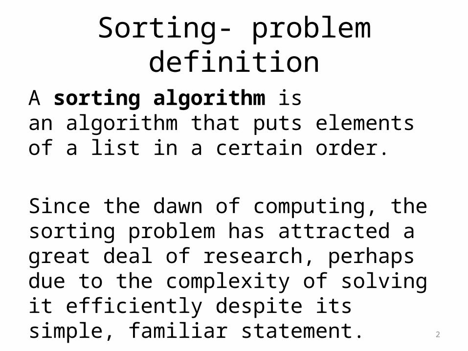
Sorting- problem definition

A sorting algorithm is an algorithm that puts elements of a list in a certain order.

Since the dawn of computing, the sorting problem has attracted a great deal of research, perhaps due to the complexity of solving it efficiently despite its simple, familiar statement.

3

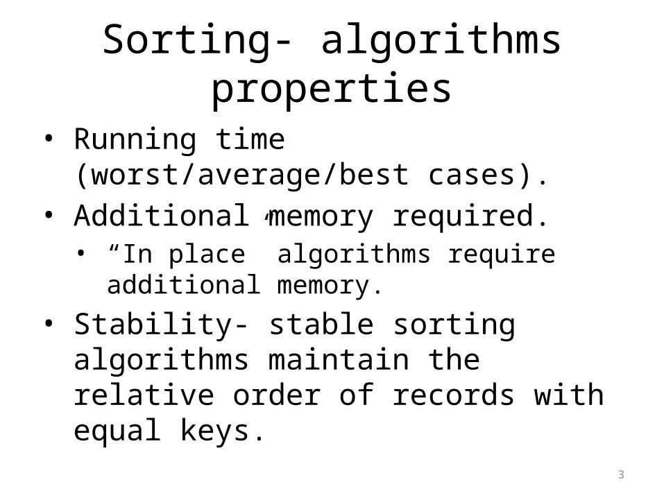
Sorting- algorithms properties

• Running time (worst/average/best cases).• Additional memory required.• “In place” algorithms require additional

memory.• Stability- stable sorting algorithms maintain

the relative order of records with equal keys.

4

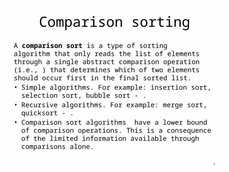
Comparison sorting

A comparison sort is a type of sorting algorithm that only reads the list of elements through a single abstract comparison operation (i.e., ) that determines which of two elements should occur first in the final sorted list.• Simple algorithms. For example: insertion sort, selection

sort, bubble sort - .• Recursive algorithms. For example: merge sort, quicksort - .• Comparison sort algorithms have a lower bound

of comparison operations. This is a consequence of the limited information available through comparisons alone.

5

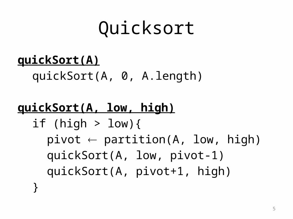
Quicksort

quickSort(A)quickSort(A, 0, A.length)

quickSort(A, low, high)if (high > low){

pivot partition(A, low, high)quickSort(A, low, pivot-1)quickSort(A, pivot+1, high)

}

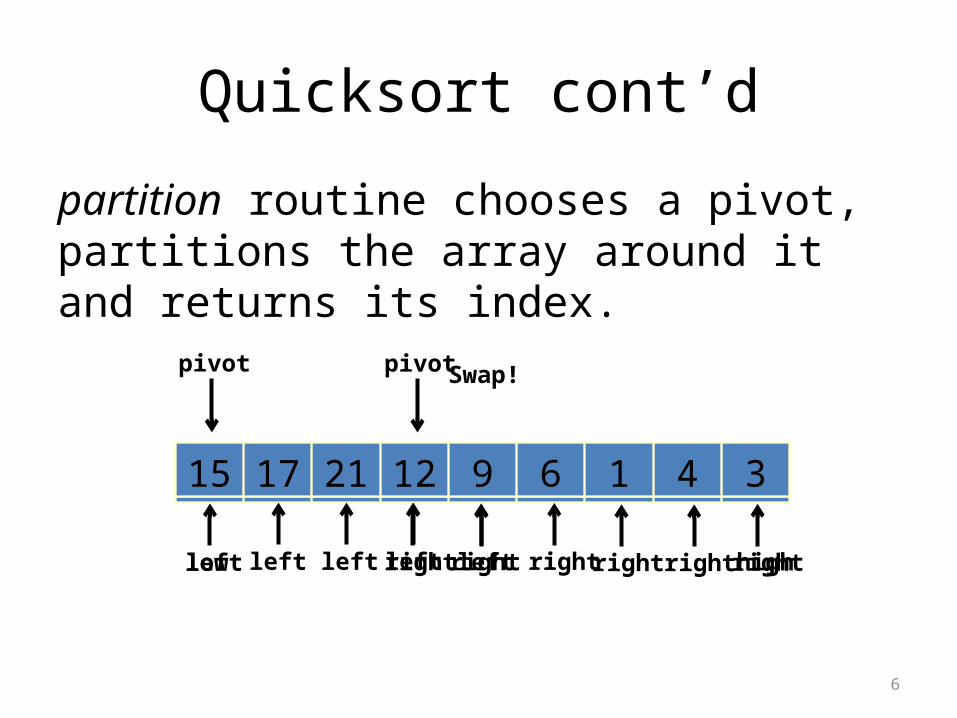
Quicksort cont’d

partition routine chooses a pivot, partitions the array around it and returns its index.

6

4 17 21 12 3 9 1 15 615 17 21 12 3 9 1 4 6

low

pivot

highleft rightleft

Swap!

left left rightrightrightright

15 17 21 12 9 3 1 4 6

rightleft

15 17 21 12 9 6 1 4 3

pivot

7

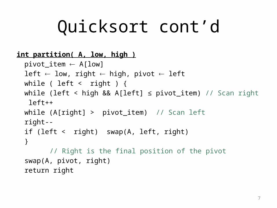
Quicksort cont’dint partition( A, low, high )

pivot_item A[low]left low, right high, pivot leftwhile ( left < right ) {

while (left < high && A[left] ≤ pivot_item) // Scan right left++

while (A[right] > pivot_item) // Scan leftright--

if (left < right) swap(A, left, right) } // Right is the final position of the pivot

swap(A, pivot, right)return right

8

Quicksort cont’d

Run-time complexity analysis• Partition on each step costs .• Best case scenario- chosen pivot is a median

(or close). Then , and the solution is .• Worst case scenario- pivot is the min/max

key. Then , and the solution is .

9

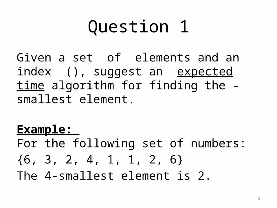
Question 1

Given a set of elements and an index (), suggest an expected time algorithm for finding the -smallest element.

Example: For the following set of numbers: {6, 3, 2, 4, 1, 1, 2, 6} The 4-smallest element is 2.

10

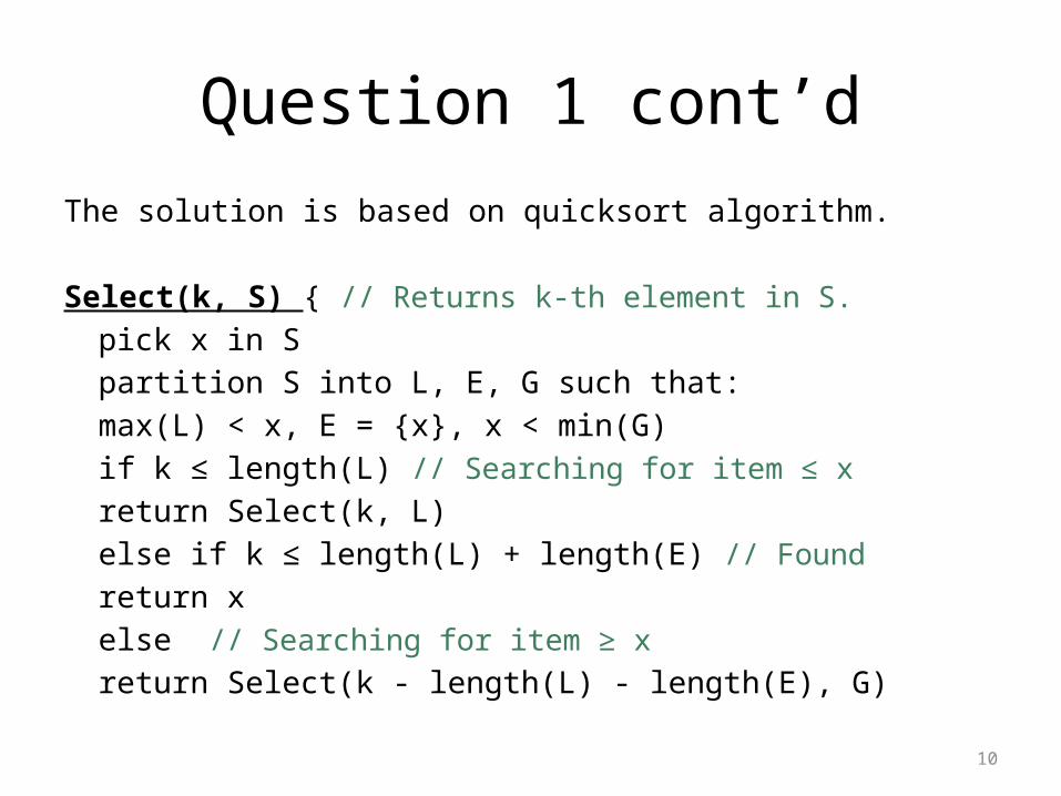
Question 1 cont’dThe solution is based on quicksort algorithm.

Select(k, S) { // Returns k-th element in S.pick x in Spartition S into L, E, G such that:max(L) < x, E = {x}, x < min(G)if k ≤ length(L) // Searching for item ≤ xreturn Select(k, L)else if k ≤ length(L) + length(E) // Foundreturn xelse // Searching for item ≥ xreturn Select(k - length(L) - length(E), G)

11

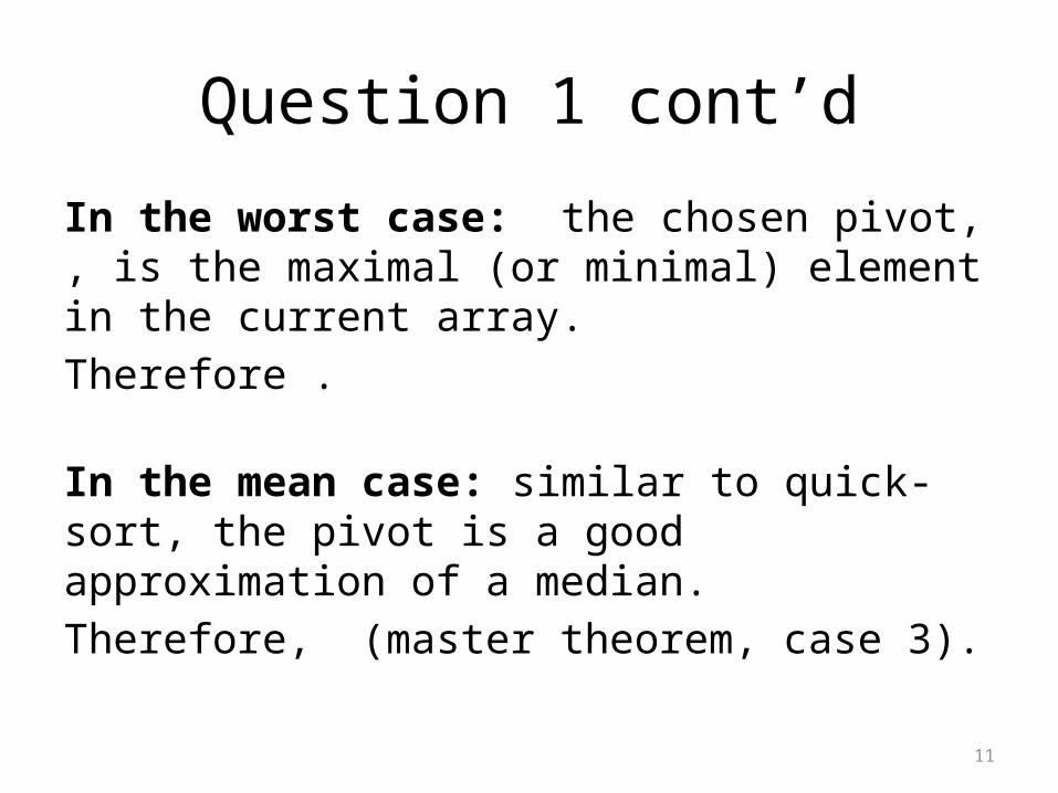
Question 1 cont’d

In the worst case: the chosen pivot, , is the maximal (or minimal) element in the current array. Therefore .

In the mean case: similar to quick-sort, the pivot is a good approximation of a median.Therefore, (master theorem, case 3).

12

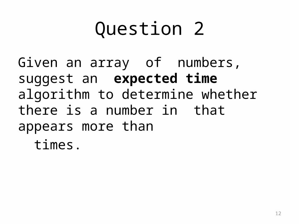
Question 2

Given an array of numbers, suggest an expected time algorithm to determine whether there is a number in that appears more than times.

13

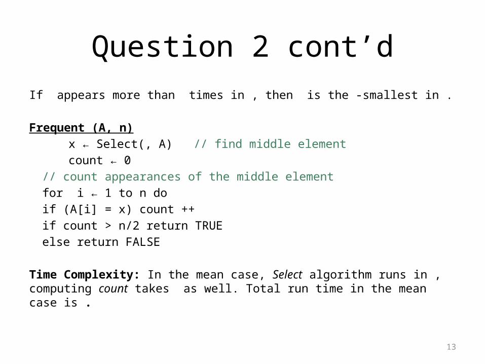
Question 2 cont’dIf appears more than times in , then is the -smallest in .

Frequent (A, n) x ← Select(, A) // find middle element count ← 0

// count appearances of the middle elementfor i ← 1 to n do if (A[i] = x) count ++if count > n/2 return TRUEelse return FALSE

Time Complexity: In the mean case, Select algorithm runs in , computing count takes as well. Total run time in the mean case is .

14

Question 2 cont’d

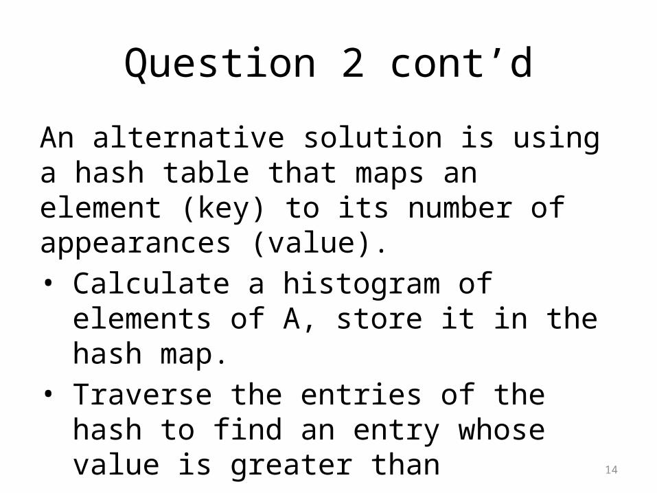
An alternative solution is using a hash table that maps an element (key) to its number of appearances (value).• Calculate a histogram of elements of A, store

it in the hash map.• Traverse the entries of the hash to find an

entry whose value is greater than • Average running time is .

15

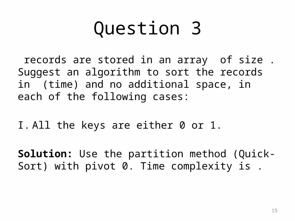
Question 3

records are stored in an array of size .Suggest an algorithm to sort the records in (time) and no additional space, in each of the following cases:

I. All the keys are either 0 or 1.

Solution: Use the partition method (Quick-Sort) with pivot 0. Time complexity is .

16

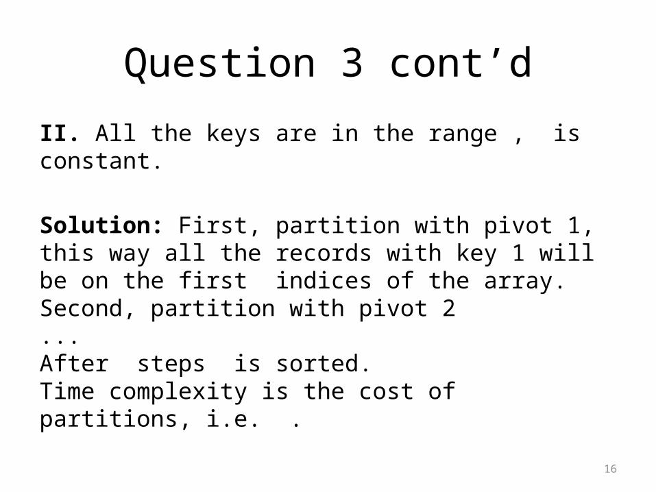
Question 3 cont’d

II. All the keys are in the range , is constant.

Solution: First, partition with pivot 1, this way all the records with key 1 will be on the first indices of the array.Second, partition with pivot 2...After steps is sorted.Time complexity is the cost of partitions, i.e. .

17

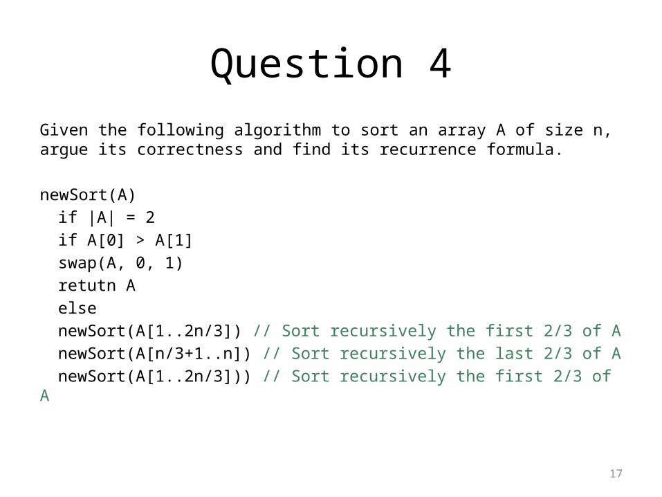
Question 4

Given the following algorithm to sort an array A of size n, argue its correctness and find its recurrence formula.

newSort(A)if |A| = 2

if A[0] > A[1] swap(A, 0, 1)

retutn Aelse

newSort(A[1..2n/3]) // Sort recursively the first 2/3 of AnewSort(A[n/3+1..n]) // Sort recursively the last 2/3 of AnewSort(A[1..2n/3])) // Sort recursively the first 2/3 of A

18

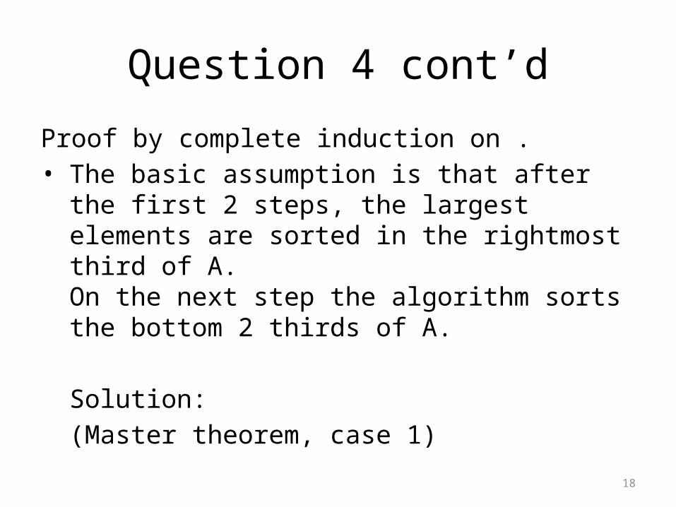
Question 4 cont’d

Proof by complete induction on . • The basic assumption is that after the first 2

steps, the largest elements are sorted in the rightmost third of A.On the next step the algorithm sorts the bottom 2 thirds of A.

Solution: (Master theorem, case 1)