


Languages
Pages
Legal

Flattening via Multi-Dimensional Scaling
Ron Kimmel
www.cs.technion.ac.il/~ron
Computer Science Department
Geometric Image Processing Lab
Technion-Israel Institute of Technology

On isometric surfaces and bending invariant signatures.
Multi-dimensional scaling techniques: Classical. Least squares. Fast.
Surface classification: experimental results.
Outline
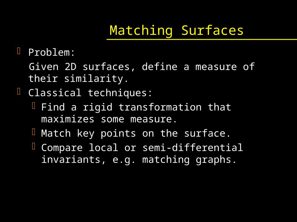
Matching Surfaces
Problem: Given 2D surfaces, define a measure of their
similarity. Classical techniques:
Find a rigid transformation that maximizes some measure.
Match key points on the surface. Compare local or semi-differential invariants,
e.g. matching graphs.
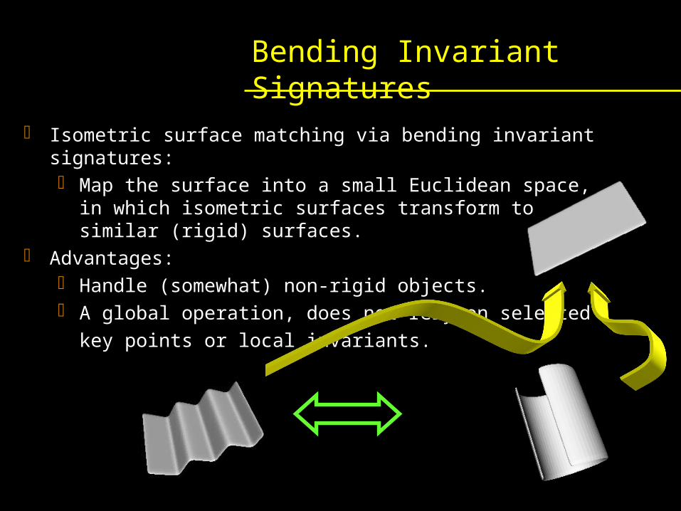
Isometric surface matching via bending invariant signatures: Map the surface into a small Euclidean space, in which
isometric surfaces transform to similar (rigid) surfaces.
Advantages: Handle (somewhat) non-rigid objects. A global operation, does not rely on selected
key points or local invariants.
Bending Invariant Signatures

Bending invariant signatures Basic Concept
Input – a surface in 3D
Extract from [D] coordinates in an m dimensional Euclidean space via
Multi-Dimensional Scaling (MDS).
Output – A 2D surface embedded in in R (for some small
m)
i j
ij ij
ij
Compute geodesic distance matrix [D] between each pair of vertices
δ = geodesic_distance(vertex ,vertex )
[D] = δ
m
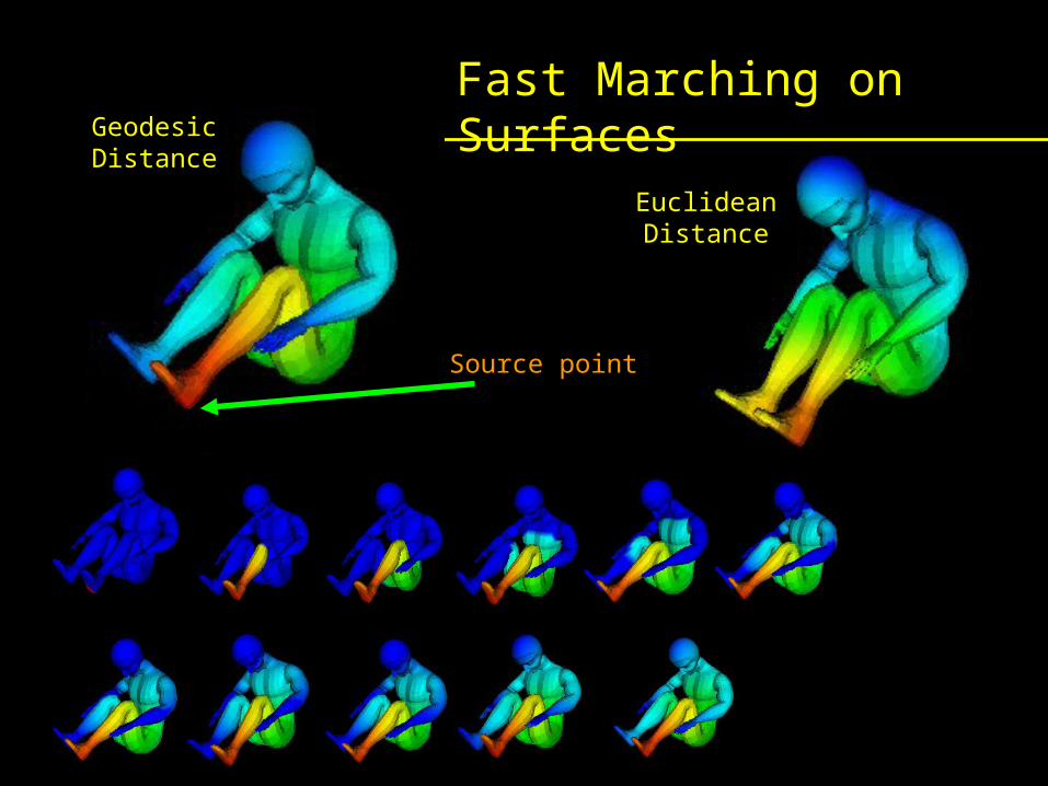
Fast Marching on Surfaces
Source point
Euclidean Distance
Geodesic Distance

Multi-Dimensional Scaling
MDS is a family of methods that map similarity measurements among objects, to points in a small dimensional Euclidean space.
The graphic display of the similarity measurements provided by MDS enables to explore the geometric structure of the data. ix
Stress =
Σ(δ - d )ij ij
2
Σδij
MDS Dissimilarity measures
coordinates in m-dimensional Euclidean Space
Stress Function
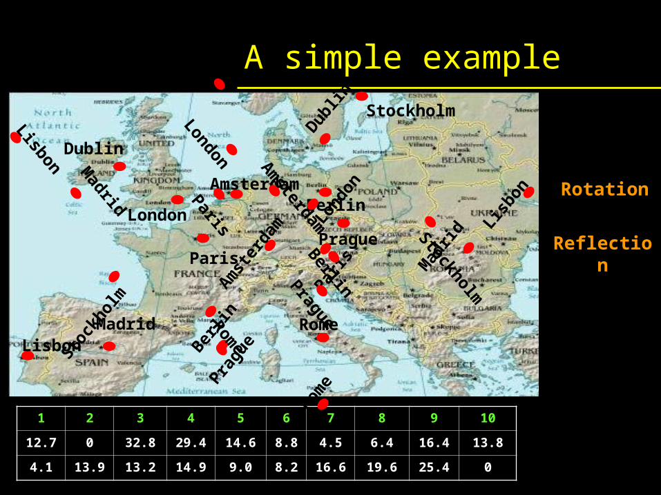
A simple example1 2 3 4 5 6 7 8 9 10
1. London 0
2. Stockholm
569 0
3. Lisbon 667 1212
0
4. Madrid 530 1043
201 0
5. Paris 141 617 596 431 0
6. Amsterdam
140 446 768 608 177 0
7. Berlin 357 325 923 740 340 218
0
8. Prague 396 423 882 690 337 272
114 0
9. Rome 569 787 714 516 436 519
472 364 0
10. Dublin 190 648 714 622 320 302
514 573 755
01 2 3 4 5 6 7 8 9 10
12.7 0 32.8 29.4 14.6 8.8 4.5 6.4 16.4 13.8
4.1 13.9 13.2 14.9 9.0 8.2 16.6 19.6 25.4 0
x
Y Stockholm
London
Dublin
Lisbon
Amsterdam
ParisPrague
Berlin
RomeMadrid
Stoc
khol
m
Lond
on
Dub
lin
Lisb
on
Am
ster
dam
Paris
Prag
ueBerlin
Rom
e
Mad
ridStockholm
London
Dublin
Lisbon Am
sterda
mParis
PragueBerlin
Rom
e
Madrid
Rotation
Reflection

Flattening via MDS Compute geodesic distances between pairs of
points. Construct a square distance matrix of
geodesic distances^2. Find the coordinates in the plane via multi-
dimensional scaling. The simplest is `classical scaling’.
Use the flattened coordinates for texturing the surface, while preserving the
texture features. Zigelman, Kimmel, Kiryati, IEEE TVCG 2002
Grossmann, Kiryati, Kimmel, IEEE TPAMI 2002
Bending invariant surface matchingElad (Elbaz), Kimmel CVPR 2001
00
0

Flattening

Flattening

Distances - comparison
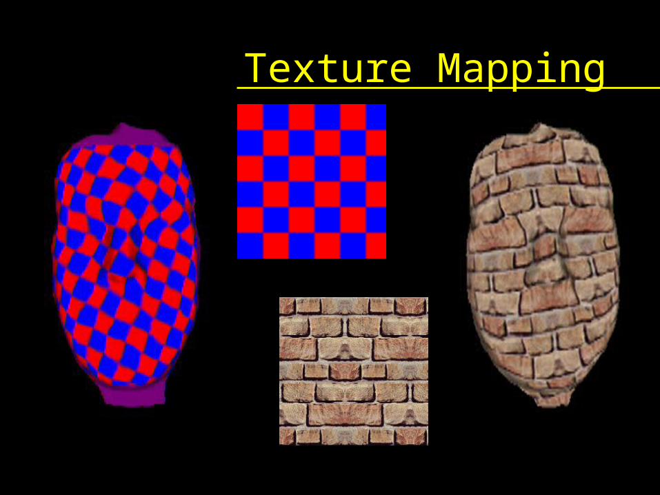
Texture Mapping
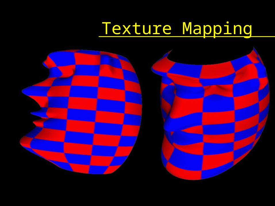
Texture Mapping
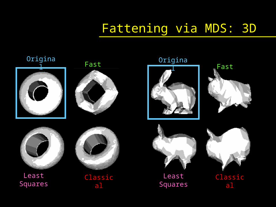
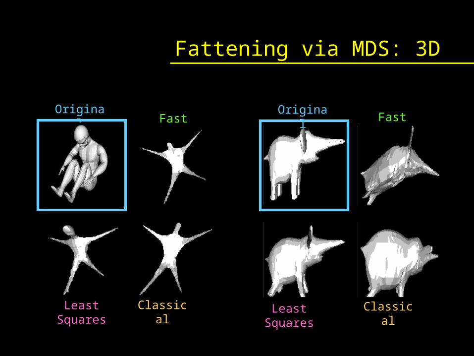
Fattening via MDS: 3D
OriginalFast
ClassicalLeast Squares
OriginalFast
Least Squares
Classical
Fattening via MDS: 3D
OriginalFast
ClassicalLeast Squares
OriginalFast
Least Squares
Classical
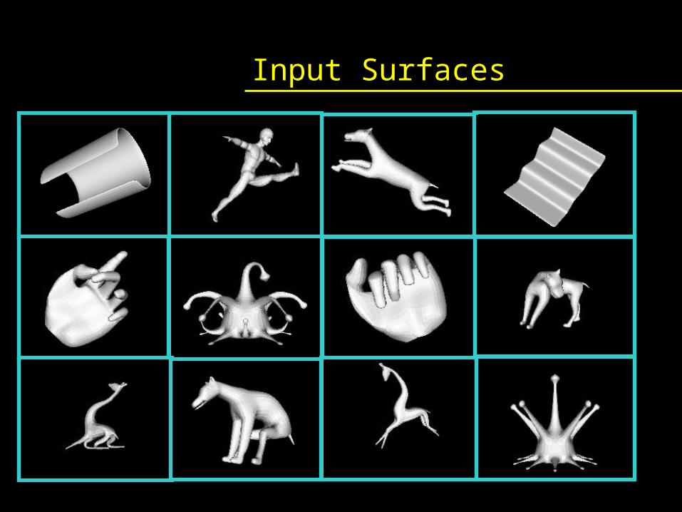
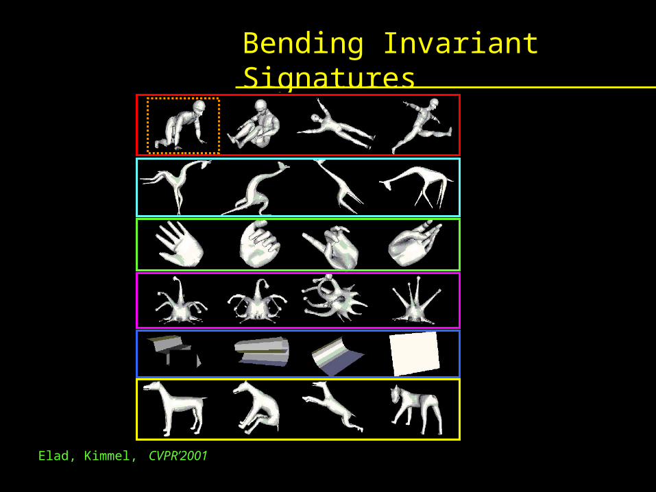
Input Surfaces
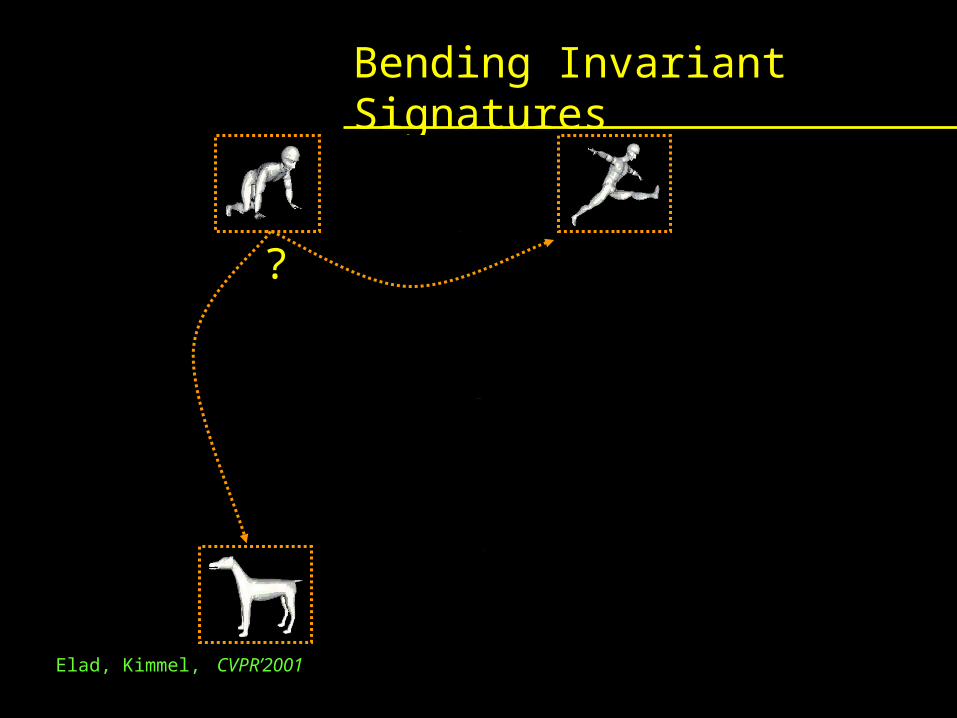
Bending Invariant Signatures
Elad, Kimmel, CVPR’2001
?
Bending Invariant Signatures
?
Elad, Kimmel, CVPR’2001

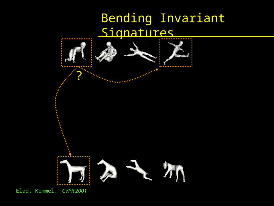
Bending Invariant Signatures
?
Elad, Kimmel, CVPR’2001

Bending Invariant Signatures
Elad, Kimmel, CVPR’2001
Bending Invariant Signatures
Elad, Kimmel, CVPR’2001
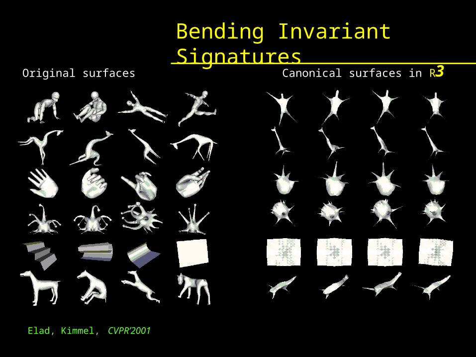
Bending Invariant Signatures
3Original surfaces Canonical surfaces in R
Elad, Kimmel, CVPR’2001

00.2
0.40.6
0.81
00.2
0.40.6
0.810
0.1
0.2
0.3
0.4
0.5
0.6
0.7
0.8
CCCC
AAAA
D
DDD
BBBB
EEEE
FFFF
00.2
0.40.6
0.81
00.2
0.40.6
0.810
0.1
0.2
0.3
0.4
0.5
0.6
0.7
0.8
CE
CC
B
A
DE
EE
B
C
A
B
D
B
F
DAD
F
A
FF
Bending Invariant Clustering
2nd moments based MDS for clustering
Original surfaces Canonical forms
*A=human body*B=hand*C=paper*D=hat*E=dog*F=giraffe
Elad, Kimmel, CVPR’2001
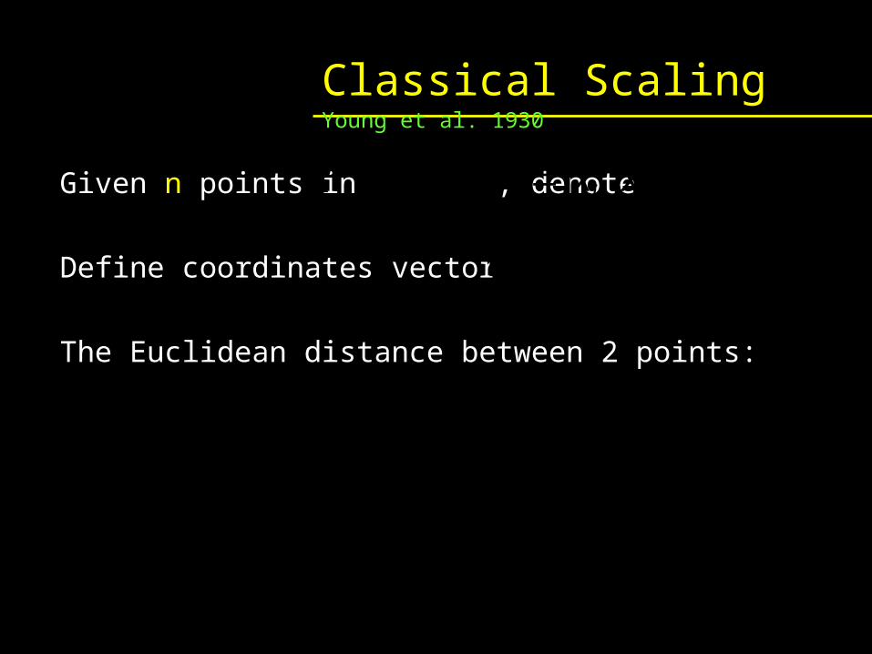
Classical Scaling Young et al.
1930
Given n points in , denote
Define coordinates vector
The Euclidean distance between 2 points:
22
1
22
1
222
2
2
jjii
k
l
lj
lj
li
li
k
l
lj
lijiij xxxxxxd
pppp
pp
T
Tp ],...,,[ 21 kiiii xxxkR
TpppP ],...,,[ 21 n

Define the `centering’ matrix where
Let the matrix
We have that and also
Thus,
Classical Scaling
Tn 11IJ 1
T
n
,...,, ][1 111
222
2
2
2
2
2
2
2
1
2
1
2
1
...
......
...
...
nnn ppp
ppp
ppp
Qnn
TTT
TT
PP00JJPPJJQJQJ
JPPQQJJDJ~~
22
)2(
0QJ 0JQQJ TT

Classical Scaling
The coordinates are related to by Thus the operation is also called `double centering’.Applying SVD, we can compute where and the coordinates can be extracted asIf we choose to take only part of the eignstructure,
then, our approximation minimizes the Frobenius norm
TPPJDJ~~
21
P~
P 1~
1
n
m
lm
li
li x
nxx
TUUJDJ 21
21UP ~
F
TUU ̂
IUUT
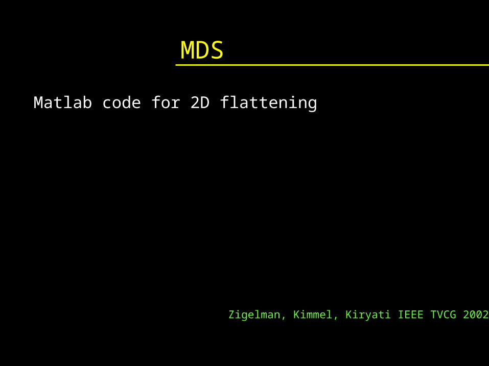
MDS
Matlab code for 2D flattening
);2(:,*)).2,2((
);1(:,*)).1,1((
);'',2,(],[
;***5.0
;/).()(
QLsqrtnewx
QLsqrtnewy
LMBeigsLQ
JDJB
nnonesneyeJ
Zigelman, Kimmel, Kiryati IEEE TVCG 2002
Classical Scaling
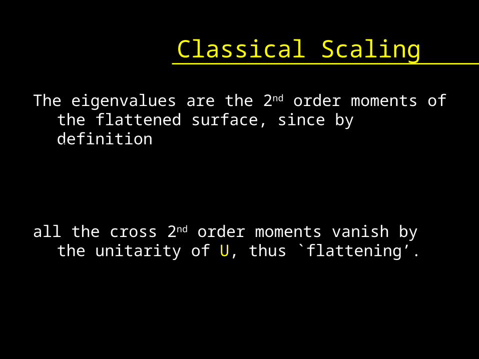
The eigenvalues are the 2nd order moments of the flattened surface, since by definition
all the cross 2nd order moments vanish by the unitarity of U, thus `flattening’.
iiii
n
m
im iiiix
TTUUUU :],[:],[:],[:],[~ 2121
1
2

Conclusions A method for bending invariant signatures Based on:
Fast marching on surfaces MDS LS/Classical/Fast
Results: Texture mapping Bending invariant signatures Classification of isometric surfaces.
00.2
0.40.6
0.81
00.2
0.40.6
0.810
0.1
0.2
0.3
0.4
0.5
0.6
0.7
0.8
CCCC
AAAA
DDDD
BBBB
EEEE
FFFF
00.2
0.40.6
0.81
00.20.40.6
0.810
0.1
0.2
0.3
0.4
0.5
0.6
0.7
0.8
CE
CC
B
ADE
EE
B
C
A
B
D
B
F
DA
D
F
A
FF
Least Squares MDS
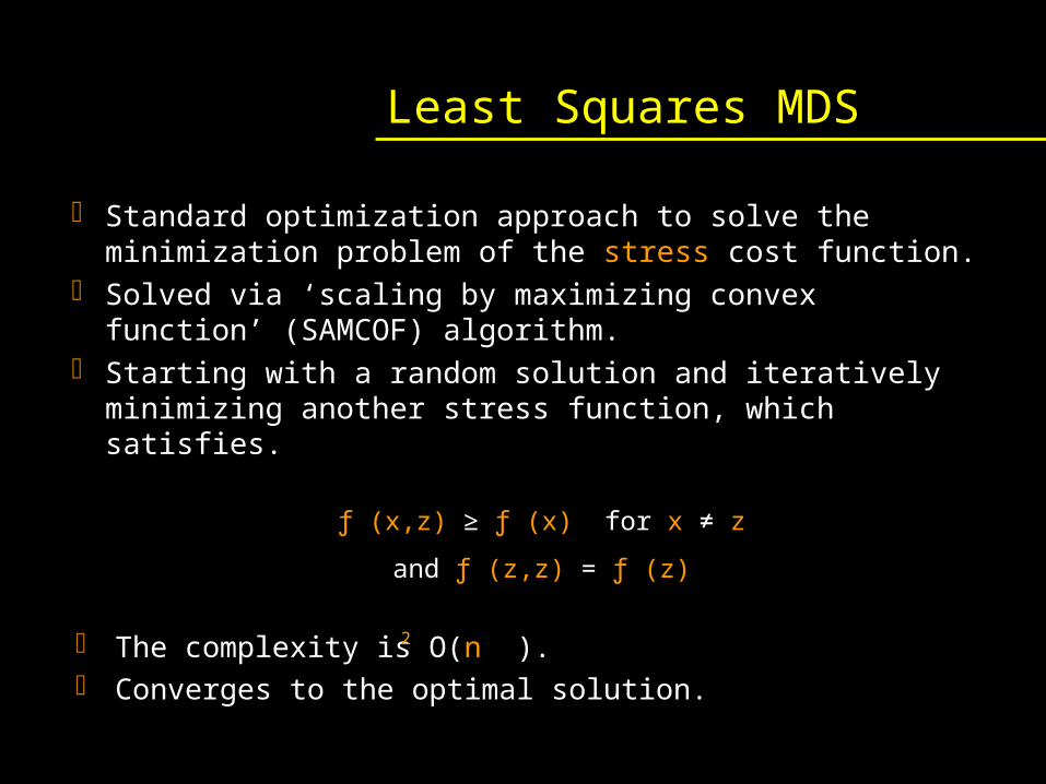
Standard optimization approach to solve the minimization problem of the stress cost function.
Solved via ‘scaling by maximizing convex function’ (SAMCOF) algorithm.
Starting with a random solution and iteratively minimizing another stress function, which satisfies.
ƒ (x,z) ≥ ƒ (x) for x ≠ z
and ƒ (z,z) = ƒ (z)
The complexity is O(n ). Converges to the optimal solution.
2

Fast MDS
The fast MDS: heuristic efficient technique O(mn). Works recursively by generating a new dimension at each step, Providing m-dimensional coordinates after m recursion steps. Project the vertices on a selected ‘line’.
First, the algorithm selects the Farthest two vertices. Next, all other vertices are projected On that line using the cosine law. Next step is to project all items to An (n-1) hyper plane (H) that is Perpendicular to the line that Connects those vertices. Generate a new distance matrix. Repeat the last three steps m times.
Top Related