


Languages
Pages
Legal

WP/15/59
Fiscal Decentralization and the Efficiency of
Public Service Delivery
Moussé Sow and Ivohasina F. Razafimahefa
© 2015 International Monetary Fund WP/15/59
IMF Working Paper
Fiscal Affairs Department
Fiscal Decentralization and the Efficiency of Public Service Delivery
Prepared by Moussé Sow and Ivohasina F. Razafimahefa1
Authorized for distribution by Bernardin Akitoby
March 2015
Abstract
This paper explores the impact of fiscal decentralization on the efficiency of public service
delivery. It uses a stochastic frontier method to estimate time-varying efficiency coefficients
and analyzes the impact of fiscal decentralization on those efficiency coefficients. The
findings indicate that fiscal decentralization can improve the efficiency of public service
delivery but only under specific conditions. First, the decentralization process requires
adequate political and institutional environments. Second, a sufficient degree of expenditure
decentralization seems necessary to obtain favorable outcomes. Third, decentralization of
expenditure needs to be accompanied by sufficient decentralization of revenue. Absent those
conditions, fiscal decentralization can worsen the efficiency of public service delivery.
JEL Classification Numbers: C16, C26, H50, H77
Keywords: Decentralization, efficiency, stochastic frontier analysis
Authors’ E-Mail Addresses: [email protected] and [email protected]
1 The authors are grateful to B. Akitoby, M. De Broeck, J.L. Combes, V. Gaspar, F. Grigoli, S. Gupta,
M. Marinkov, A. Minea, A. Schaechter and participants in the IMF Fiscal Affairs Department seminar for their
useful comments.
This Working Paper should not be reported as representing the views of the IMF.
The views expressed in this Working Paper are those of the author(s) and do not necessarily
represent those of the IMF or IMF policy. Working Papers describe research in progress by the
author(s) and are published to elicit comments and to further debate.

2
Contents Page
I. Introduction ............................................................................................................................3
II. Literature Review and Theoretical Background ...................................................................3
III. Empirical Analysis ...............................................................................................................5
A. Methodology .............................................................................................................5 B. Data ...........................................................................................................................8 C. Efficiency Estimates ................................................................................................10 D. Direct Channel and Non-Linear Relationship .........................................................11 E. Political and Institutional Conditions ......................................................................13
F. Robustness ...............................................................................................................16
G. Revenue Decentralization .......................................................................................20
IV. Conclusions and Policy Implications.................................................................................22
Tables
1. Descriptive Statistics ............................................................................................................10 2. Stochastic Frontier Estimates of Public Service Efficiency ................................................10 3. Fiscal Decentralization and Public Expenditure Efficiency ................................................12
4. Fiscal Decentralization and Public Expenditure Efficiency (Non-linearity) .......................13 5. Fiscal Decentralization and Political/Institutional Environments........................................15
6. Fiscal Decentralization and Political/Institutional Environments (Sub-groups) .................15 7. Fiscal Decentralization and Public Expenditure Efficiency: Excluding Outliers ................16
8. Fiscal Decentralization and Public Expenditure Efficiency: Alternative
Efficiency Estimates ..........................................................................................................18
9. Fiscal Decentralization and Public Expenditure Efficiency: Absorbing
Short-Term Fluctuations ....................................................................................................19 10. Fiscal Decentralizatiojn and Public Expenditure Efficiency: Alternative
Political and Institutional Variables ...................................................................................19 11. Revenue Decentralization: Baseline and Country-Specific Estimates ..............................20 12. Revenue Decentralization: Alternative Efficiency Estimates ............................................21
13. Revenue Decentralization: Excluding Outliers ..................................................................21 14. Revenue Decentralization: Political/Institutional Interactions ..........................................22
Figure
1. Share of Subnational Government Expenditure/Revenue .....................................................9
References ...............................................................................................................................23
Annexes
I. Countries, Data Coverage, and Sources ...............................................................................27 II. Variables, Definition and Data Sources ..............................................................................28
III. Alternative Policy Outcome Variables ..............................................................................29
3
I. INTRODUCTION
This paper analyzes the impacts of fiscal decentralization on the efficiency of public
service delivery. It contributes to existing studies by focusing explicitly on the efficiency of
public service delivery instead of the policy outcome. The policy outcome can be improved by
augmenting policy inputs (for instance, spending allocation); in contrast, efficiency is measured
as the difference in policy outcomes—across countries and over time—under a similar set of
policy inputs. This paper also covers a large sample of countries, including developed,
emerging, and developing economies.2 Last, it uses recent empirical techniques to reach the
findings and ascertain their robustness.
The paper’s findings suggest that fiscal decentralization can serve as a policy tool to
improve performance, but only under specific conditions. Our findings focus on the
efficiency of spending on education and health and indicate that an adequate institutional
environment is needed for decentralization to improve public service delivery. Such conditions
include effective autonomy of local governments, strong accountability at various levels of
institutions, good governance, and strong capacity at the local level. Moreover, a sufficient
degree of expenditure decentralization seems necessary to obtain a positive outcome. And
finally, decentralization of expenditure needs to be accompanied by sufficient decentralization
of revenue to obtain favorable outcomes. Absent those conditions, fiscal decentralization can
worsen the efficiency of public service delivery. The paper is structured as follows. Section II
reviews the existing literature and summarizes the merits and risks of fiscal decentralization.
Section III presents the empirical analysis. Section IV concludes with the main policy
recommendations.
II. LITERATURE REVIEW AND THEORETICAL BACKGROUND
Fiscal decentralization can improve the efficiency of public service delivery through
preference matching and allocative efficiency. Local governments possess better access to
local preferences and, consequently, have an informational advantage over the central
government in deciding which provision of goods and services would best satisfy citizens’
needs (Hayek, 1945; Tiebout, 1956; Musgrave, 1969). When provided by the jurisdiction that
has the control over the minimum geographic area, costs and benefits of public services are
fully internalized, which is expected to improve allocative efficiency (Oates, 1972).
Fiscal decentralization can also ameliorate efficiencies by fostering stronger
accountability. Geographical closeness of public institutions to the local population (final
beneficiaries) fosters accountability and can improve public service outcomes, particularly in
social sectors such as education and health (Ahmad, Brosio, and Tanzi, 2008; Cantarero and
2 Previous studies focused solely on a specific country or a specific group of countries.
4
Pacual Sanchez, 2006). Local accountability is expected to put pressure on local authorities to
continuously search for ways to produce and deliver better public service under limited
resources, leading to “productive effeciency.” Accountability can foster larger spending in
public investment and in growth-enhancing sectors, such as education and health (Keen and
Marchand, 1997; Arze del Granado and others, 2005; Bénassy-Quéré and others, 2007;
Kappeler and Valila, 2008; Fredriksen, 2013). Local accountability can be strengthened through
a direct election of local authorities by the local population.
Furthermore, fiscal decentralization can improve efficiency through the “voting with one’s
feet” hypothesis. Decentralization gives voters more electoral control over the authorities
(Seabright, 1996; Persson and Tabellini, 2000; Hindriks and Lockwood, 2005). It encourages
competition across local governments to improve public services; voters can use the
performance of neighboring governments to make inferences about the competence or
benevolence of their own local politicians (Bordignon and others, 2004). Fiscal decentralization
may lead to a decrease in lobbying by interest groups, distorting policy choices and increasing
waste of public funds.
However, fiscal decentralization can worsen public service delivery if scale economy is
important. Devolution of public service delivery to a small-scale local government can
decrease efficiency and increase costs if economies of scale are important in the process of
production and provision of some specific public goods. For instance, shifting the production
and provision of public services to a municipality with a small size of government officials
(producers and providers) and a small population (beneficiaries) can reduce efficiency.
Fiscal decentralization can also obstruct the redistribution role of the central government.
To guarantee a minimum level of public service and basic needs (or standard of living) for the
entire population (regardless of their geographical location), the central government often
carries out equalization transfers, which would be disrupted in cases of insufficient leverage on
resources (Ter-Minassian, 1997). When a large share of revenue and expenditure is shifted to
local governments, the central government does not possess sufficient resources to ensure a
minimum equity across the entire territory.
Fiscal decentralization can also hinder public service delivery if accountability is loose. If
accountability is not broadly anchored in a local democratic process, but instead is based on
rent-seeking political behavior, local governments would be tempted to allocate higher
decentralized expenditure to non-productive expenditure items (such as wages and goods and
services instead of capital expenditure). This can hinder efficiency, economic growth, and
overall macroeconomic performance (Davoodi and Zou, 1998; Woller and Phillips, 1998;
Zhang and Zou, 1998; Rodriguez-Pose and others, 2009; Gonzalez Alegre, 2010; Grisorio and
Prota, 2011).
5
III. EMPIRICAL ANALYSIS
A. Methodology
This paper investigates the efficiency, rather than just the outcome, of public service
delivery in health and education. Policy outcome is the directly measurable impact of public
service delivery; outcome indicators can include infant mortality rate and school enrollment
rate. Policy outcomes can be improved by augmenting policy inputs, such as expenditure
allocation for health and education. However, the efficiency analysis focuses on the
improvement in outcome while keeping inputs unchanged.3 This approach allows analyzing the
impact of policies other than inputs in improving the provision of public goods and services;
such policies can include fiscal decentralization.
The methodology is based on a two-step approach, estimating efficiency coefficients and
analyzing the impact of fiscal decentralization on the latter. In a first step, the efficiency of
public service delivery is estimated using stochastic frontier techniques. These techniques
provide time-varying coefficients that measure the distance of the public services in a specific
country at a specific year to the best public services provided using similar inputs in the sample
of countries considered in this analysis. In a second step, this paper estimates the effects of
fiscal decentralization on the estimated efficiencies. Instrumental variable methods are used to
obtain bias-corrected coefficients. These methods address concerns about endogeneity
associated with the decentralization process; they can also tackle reverse causality that could
plague the estimated parameters.
In a first step, efficiency coefficients are estimated from stochastic frontier techniques.
Methodologies on efficiency estimates can be grouped in two main approaches: (i) a parametric
approach (Battese and Coelli, 1988; Jayasuriya and Wodon, 2003; Grigoli and Kapsoli, 2013)
and (ii) a non-parametric approach (Gupta and Verhoeven, 2001; Herrera and Pang, 2005;
Gupta and others, 2007). This paper uses the parametric approach-based stochastic frontier
analysis (SFA). The SFA allows estimating models with multiple inputs, as opposed to non-
parametric models that do not take into account the effect of exogenous factors on the outcome
variable because of the restriction on the number of variables. As the outcome variables in this
paper, that is, infant mortality and enrollment ratio, are plausibly affected by structural factors
other than public expenditure, such as socioeconomic characteristics of the country, a
multivariable model is better suited for the analysis. Moreover, the SFA allows estimating
country-specific and time-varying coefficients.
The SFA techniques assume that no economic agent (i.e., country) can exceed the ideal
“frontier.” The frontier refers to the optimum output—infant mortality rate or enrollment
rate—produced with limited inputs, such as public expenditure. The deviation of the output in a
3 Alternatively, the efficiency analysis can also aim at reducing inputs while keeping the outcome unchanged.
6
specific country at a specific time from this frontier represents the individual measure of
efficiency of that country. Efficient governments are those operating at, or very close to, the
frontier as they try to reduce the infant mortality rate or improve the enrollment rate, given a
limited amount of public expenditure.
The first-step model is specified as follows:
1 , 1
1
1K
it it k k it it
k
Y PE Z
2 and exp
it it it
it i ig t g t t T
The dependent variable itY in equation (1) represents public expenditure outcomes on health and
education, namely the infant mortality rate and the secondary school enrollment rate, with
subscripts i and t denoting respectively country and time dimensions. The interest variable
1itPE corresponds to public expenditure on health and education as a percent of GDP. A set of
control variables ,k itZ are added and are likely to influence the infant mortality rate or the
enrollment rate. The error term it in equation (1) has two components as shown in equation (2);
it represents an idiosyncratic disturbance, capturing measurement error or any other classical
noise, and the remaining part it is a one-sided disturbance capturing the country-specific and
time-varying efficiencies of public expenditure.4 Equations (1) and (2) allow obtaining the
country-specific and time-varying efficiencies of public expenditure, following the formula
provided by Battese and Coelli (1988) and Jondrow and others (1988).
The second step consists of measuring the extent to which fiscal decentralization affects
the estimated efficiencies. The impact of fiscal decentralization is analyzed through a direct
channel, a non-linear relationship, and interactions with political and institutional variables. The
baseline model is the following:
1 1ˆ 3it it it itfd GDP
The dependent variable ˆit is the country-specific and time-varying efficiencies estimated from
equations (1) and (2), α is a common constant term, and 1itfd measures fiscal decentralization.
4 A stream of existing literature assumes time-invariant efficiency. However, the assumption of invariant efficiency
might be questionable, especially in the presence of long panel data. We relax the assumption of time-invariant
efficiency and allow for time-varying individual-specific efficiencies (Cornwell and others, 1990).
7
To explore non-linearities in the relationship between fiscal decentralization and public
expenditure efficiency, a quadratic specification is added—i.e., squared fiscal decentralization
2
1itfd —as shown in equation (4). Non-linearities, if any, are detected by computing the
derivatives:
2
1 1 2 1 1ˆ 4it it it it itfd fd GDP
Furthermore, the impact of the political and institutional environment on the relationship
between decentralization and the efficiency of public service delivery is investigated. Political
and institutional variables are introduced additively ( 1itI ) but also in interaction with fiscal
decentralization 1 1it itfd I , as shown in equation (5).
1 1 1 1 1ˆ 5it it it it it it itfd fd I I GDP
Parameter corresponds to the direct effect of political and institutional variables on
efficiency. Parameters and correspond respectively to the effect of fiscal decentralization on
the efficiency and the influence of the political and institutional environments on the causal link
between fiscal decentralization and public service efficiency. it in equations (3)–(5) is a
composite error term, taking into account country-specific characteristics.
Fiscal decentralization is measured as the share of subnational fiscal variables over
general government fiscal variables.5 The main estimates in this paper are based on the
expenditure side of fiscal decentralization, using the share of subnational expenditure to general
government expenditure.6 The main focus is on expenditure as it is directly linked to health and
education outcomes and efficiency (as opposed to revenue). However, to ensure a
comprehensive study, the paper also analyzes the impacts of revenue decentralization on the
efficiency of public service delivery, using the share of local government revenue to general
government revenue.7 The political and institutional variables focus on the level of corruption,
the degree of autonomy of the regions, the strength of the democracy, and the constitutional
regime (presidential or parliamentary). Control variables in the stochastic frontier analysis
comprise the real GDP per capita as a measure of the level of development, the density and
population size, and the average years of primary and secondary schooling. All these variables
5 Local governments can include states, regions, districts, municipalities, and other level(s) of government,
depending on the institutional arrangement in the country.
6 Owing to difficulties in obtaining data from local and regional governments, our fiscal decentralization index is
obtained as the residual after deducting the ratio of central government share of expenditure over total general
government expenditure. This approach can have some caveats, but it allows large country and period coverages.
7 The vertical fiscal imbalance, i.e., the share of local government expenditure financed with its own revenue, can
also provide important insights; however, this indicator is not available for the full sample in this study.

8
are considered to influence the infant mortality rate and the secondary school enrollment rate.8 It
would be insightful to use the share of subnational expenditure on health and education to
general government expenditure in each of the two sectors; however, such data are not available
for many of the countries in the sample. Furthermore, the efficiency is influenced by factors
beyond expenditure, and an analysis using aggregate expenditure ratio allows clearer
comparison with the analysis using aggregate revenue ratio.
Endogeneity and causality concerns are addressed through lag and instrument techniques
that motivate the introduction of additional variables. An initial attempt at reducing any bias
consists of introducing all explanatory variables, including fiscal decentralization, with a one-
period lag. Furthermore, two-stage least squares techniques are applied for the fiscal
decentralization variable, using three instrumental variables. First, the population size is
considered a significant variable affecting the decentralization process because larger countries
generally tend to be more decentralized despite some counter examples (Dziobek et al., 2011;
Jiménez-Rubio, 2011; Escolano et al., 2012). The rationale is that in countries with large
populations, it is more difficult for central authorities to have sufficient information to target
citizens’ needs, which leads to decentralization. Second, the existence of natural resources can
act as an obstacle to decentralization, because of possible rent-seeking behaviors of fiscal
authorities that benefit directly from the resource windfalls. Under such circumstances,
embarking on a fiscal decentralization process would imply a subsequent private loss for
incumbent authorities. On the other hand, residents of resource-rich regions can claim larger
shares of resources through accelerated decentralization. Moreover, natural resources might be
seen as a blessing, triggering the decentralization process because windfalls may constitute an
additional source of revenue to share with the subnational governments. Third, government
fractionalization and fractionalization in the legislative system can affect the decentralization
process. Fractionalization is measured as the probability that two deputies randomly picked
either from the government or the legislature will be from different parties. Higher
fractionalization may either act against the decentralization process, owing to political motives,
or accelerate decentralization. The expected signs of these two last instrumental variables on the
decentralization process cannot be determined a priori.
B. Data
The sample covers an unbalanced panel of 64 countries, including advanced, emerging,
and developing economies, during 1990–2012. Data are taken from various sources, including
the IMF’s Governments Financial Statistics, the World Bank’s World Development Indicators,
Eurostat, and OCED databases, among others. Annexes I and II present the full sample, variable
definitions, and sources.
8 To avoid perfect collinearity, we exclude the variable average year of schooling while estimating the effect of
public education expenditure on the secondary school enrollment rate. GDP per capita is used as a control variable
when estimating the effect of fiscal decentralization on public expenditure efficiency.
9
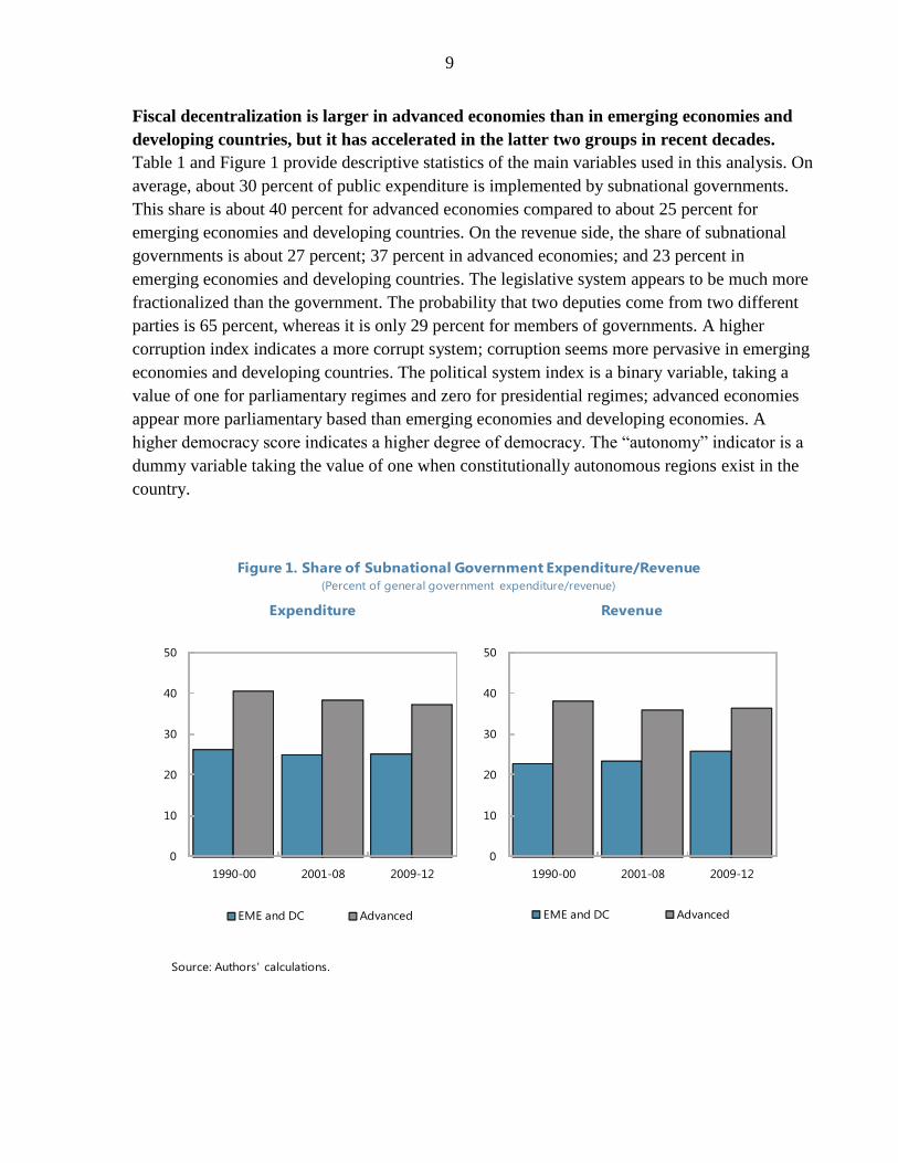
Fiscal decentralization is larger in advanced economies than in emerging economies and
developing countries, but it has accelerated in the latter two groups in recent decades.
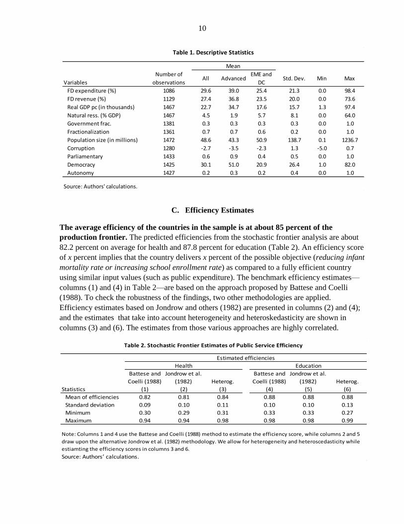
Table 1 and Figure 1 provide descriptive statistics of the main variables used in this analysis. On
average, about 30 percent of public expenditure is implemented by subnational governments.
This share is about 40 percent for advanced economies compared to about 25 percent for
emerging economies and developing countries. On the revenue side, the share of subnational
governments is about 27 percent; 37 percent in advanced economies; and 23 percent in
emerging economies and developing countries. The legislative system appears to be much more
fractionalized than the government. The probability that two deputies come from two different
parties is 65 percent, whereas it is only 29 percent for members of governments. A higher
corruption index indicates a more corrupt system; corruption seems more pervasive in emerging
economies and developing countries. The political system index is a binary variable, taking a
value of one for parliamentary regimes and zero for presidential regimes; advanced economies
appear more parliamentary based than emerging economies and developing economies. A
higher democracy score indicates a higher degree of democracy. The “autonomy” indicator is a
dummy variable taking the value of one when constitutionally autonomous regions exist in the
country.
Figure 1. Share of Subnational Government Expenditure/Revenue
(Percent of general government expenditure/revenue)
Source: Authors' calculations.
0
10
20
30
40
50
1990-00 2001-08 2009-12
EME and DC Advanced
Expenditure
0
10
20
30
40
50
1990-00 2001-08 2009-12
EME and DC Advanced
Revenue
10
C. Efficiency Estimates
The average efficiency of the countries in the sample is at about 85 percent of the
production frontier. The predicted efficiencies from the stochastic frontier analysis are about
82.2 percent on average for health and 87.8 percent for education (Table 2). An efficiency score
of x percent implies that the country delivers x percent of the possible objective (reducing infant
mortality rate or increasing school enrollment rate) as compared to a fully efficient country
using similar input values (such as public expenditure). The benchmark efficiency estimates—
columns (1) and (4) in Table 2—are based on the approach proposed by Battese and Coelli
(1988). To check the robustness of the findings, two other methodologies are applied.
Efficiency estimates based on Jondrow and others (1982) are presented in columns (2) and (4);
and the estimates that take into account heterogeneity and heteroskedasticity are shown in
columns (3) and (6). The estimates from those various approaches are highly correlated.
Variables
Number of
observationsAll Advanced
EME and
DCStd. Dev. Min Max
FD expenditure (%) 1086 29.6 39.0 25.4 21.3 0.0 98.4
FD revenue (%) 1129 27.4 36.8 23.5 20.0 0.0 73.6
Real GDP pc (in thousands) 1467 22.7 34.7 17.6 15.7 1.3 97.4
Natural ress. (% GDP) 1467 4.5 1.9 5.7 8.1 0.0 64.0
Government frac. 1381 0.3 0.3 0.3 0.3 0.0 1.0
Fractionalization 1361 0.7 0.7 0.6 0.2 0.0 1.0
Population size (in millions) 1472 48.6 43.3 50.9 138.7 0.1 1236.7
Corruption 1280 -2.7 -3.5 -2.3 1.3 -5.0 0.7
Parliamentary 1433 0.6 0.9 0.4 0.5 0.0 1.0
Democracy 1425 30.1 51.0 20.9 26.4 1.0 82.0
Autonomy 1427 0.2 0.3 0.2 0.4 0.0 1.0
Source: Authors' calculations.
Table 1. Descriptive Statistics
Mean
Battese and
Coelli (1988)
Jondrow et al.
(1982) Heterog.
Battese and
Coelli (1988)
Jondrow et al.
(1982) Heterog.
Statistics (1) (2) (3) (4) (5) (6)
Mean of efficiencies 0.82 0.81 0.84 0.88 0.88 0.88
Standard deviation 0.09 0.10 0.11 0.10 0.10 0.13
Minimum 0.30 0.29 0.31 0.33 0.33 0.27
Maximum 0.94 0.94 0.98 0.98 0.98 0.99
Source: Authors’ calculations.
Health Education
Table 2. Stochastic Frontier Estimates of Public Service Efficiency
Note: Columns 1 and 4 use the Battese and Coelli (1988) method to estimate the efficiency score, while columns 2 and 5
draw upon the alternative Jondrow et al. (1982) methodology. We allow for heterogeneity and heteroscedasticity while
estiamting the efficiency scores in columns 3 and 6.
Estimated efficiencies
11
D. Direct Channel and Non-Linear Relationship
Through a direct channel, expenditure decentralization seems to improve the efficiency of
public service delivery in advanced economies but has a negative impact in emerging
economies and developing countries. Estimating equation (3), the first step of the two-stage
least squares points to the appropriateness of the instrument variables. The latter are
significantly correlated with the endogenous regressor in almost all cases (the associated p-
values are < 0.05). Besides, using the Kleibergen-Paap’s p values, the null hypothesis that “the
equations are underidentified” can be rejected at the 5 percent level. The results of the second
step are presented in Table 3. Pooling the advanced economies, emerging markets, and
developing economies, it appears that fiscal decentralization has no significant effect on the
efficiency of public expenditure (columns 1 and 6). Considering that the various countries
exhibit dissimilar levels of decentralization (as shown in the previous section), the sample is
divided in two groups: (i) advanced economies, and (ii) emerging markets and developing
economies.9 For advanced economies, fiscal decentralization shows positive impacts on the
efficiency of public expenditure on health (column 2). To quantify this effect, one could say that
a 5 percent increase in fiscal decentralization would lead to 2.9 percentage points of efficiency
gains in public service delivery. The coefficient is statistically insignificant for education
(column 7). In contrast, for emerging markets and developing economies, the impacts are
negative (columns 3 and 8). These positive and negative effects of decentralization, respectively
for the first and second group of countries, are robust to the inclusion of time dummies, albeit
with a slight reduction in the magnitude of the parameters (columns 4,5,9, and 10). This seems
to confirm that the results are not driven by common shocks hitting all countries at the same
time, nor by a time-trend evolution of the efficiency scores.
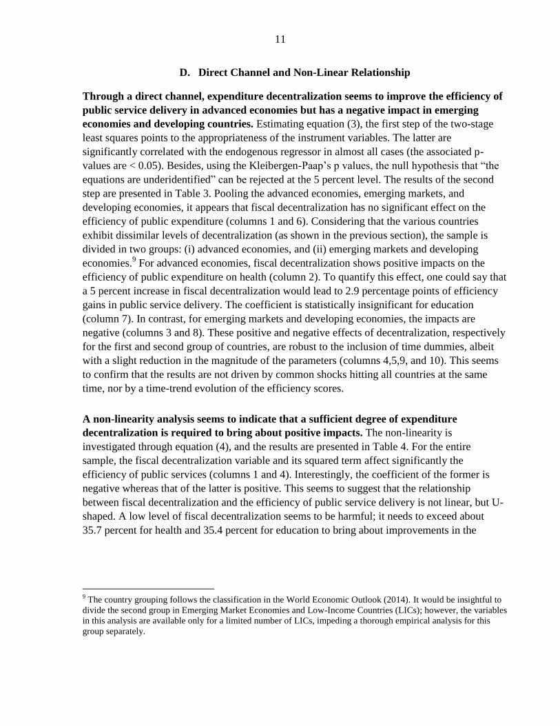
A non-linearity analysis seems to indicate that a sufficient degree of expenditure
decentralization is required to bring about positive impacts. The non-linearity is
investigated through equation (4), and the results are presented in Table 4. For the entire
sample, the fiscal decentralization variable and its squared term affect significantly the
efficiency of public services (columns 1 and 4). Interestingly, the coefficient of the former is
negative whereas that of the latter is positive. This seems to suggest that the relationship
between fiscal decentralization and the efficiency of public service delivery is not linear, but U-
shaped. A low level of fiscal decentralization seems to be harmful; it needs to exceed about
35.7 percent for health and 35.4 percent for education to bring about improvements in the
9 The country grouping follows the classification in the World Economic Outlook (2014). It would be insightful to
divide the second group in Emerging Market Economies and Low-Income Countries (LICs); however, the variables
in this analysis are available only for a limited number of LICs, impeding a thorough empirical analysis for this
group separately.

12
efficiency of public services.10
At least, about one third of public expenditure would need to be
shifted to the local authorities to obtain positive outcomes from fiscal decentralization. This
non-linear relationship might imply the importance of the scale economy in the production and
delivery of public services. As many public services require substantial initial fixed costs, if the
scale of public services shifted to the local level is too small, the local authorities might have to
reduce the provision of services to reduce the variable costs to cover the large initial fixed costs.
Note, however, that the sufficient level of fiscal decentralization likely differs across countries,
depending on country-specific considerations.
10
Based on the estimated parameters in Table 4, the decentralization indicative threshold for the health sector is
computed as 1
1 2
ˆ *
1 2 22it
itfdfd fd
or fd*
) 100=35.7 percent. The threshold for
the education sector was derived similarly.
All Advanced EME and DC All Advanced EME and DC
Variables (1) (2) (3) (4) (5) (6) (7) (8) (9) (10)
FD(t-1) 0.109 0.599*** -0.322*** 0.433*** -0.187*** 0.0373 -0.0453 -0.872** 0.800*** -0.616**
(0.925) (7.956) (-2.919) (5.211) (-2.737) (0.126) (-0.339) (-2.545) (3.674) (-2.305)
Real GDP pc(t-1) 0.035*** 0.008 0.023*** -0.061*** -0.093*** -0.020** -0.077*** -0.007 0.044 -0.070**
(5.402) (0.778) (2.730) (-3.286) (-6.865) (-2.200) (-4.339) (-0.386) (1.284) (-2.564)
Time dummies Yes Yes Yes Yes Yes Yes Yes Yes Yes Yes
Number of observations 875 269 606 269 606 690 213 477 213 477
Countries 55 14 41 14 41 53 14 39 14 39
Fisher (p-value ) 0.000 0.000 0.000 0.000 0.000 0.056 0.000 0.041 0.000 0.249
Hansen OID (p-value ) 0.000 0.008 0.000 0.000 0.007 0.000 0.000 0.004 0.042 0.000
KP-under 0.000 0.000 0.000 0.000 0.000 0.057 0.002 0.048 0.013 0.034
FD(t-1) instrumentation (p-value ) 0.000 0.000 0.000 0.000 0.000 0.052 0.000 0.029 0.019 0.029
Source: Authors’ calculations.
Table 3. Fiscal Decentralization and Public Expenditure Efficiency
Dependent variable: estimated efficiencies
Note: (*), (**) and (***) denote statistical significance level of 10%, 5% and 1% percent respectively. Robust t-statistics are shown in parentheses. Fisher
statistic presents a test of join significance of estimated coefficients. Hansen OID and Kleibergen-Paap (KP) test respectively the over-identification
restriction and the hypothesis that equations are underidentified. FD instrumentation test, with a lower p-value indicates that endogenous regressors (fiscal
decentralization) are significantly correlated with the instrumental variables proposed (political and government fractionalization, and natural resource
Health Education
Time dummies Time dummies
13
The U-shaped relationship is confirmed when the sample observations are split below and
above the indicative threshold. For health, when the fiscal decentralization ratio is below the
estimated indicative threshold of 35.7 percent, a 1 percent increase in fiscal decentralization
ratio reduces the efficiency by about 0.8 percentage point (column 2 of Table 4). In contrast,
when the decentralization ratio reaches or exceeds the indicative threshold, decentralization
improves the efficiency of public service delivery. A 1 percent increase in the decentralization
ratio increases the efficiency by 0.2 percentage point (column 3 of Table 4). For education, the
coefficients of the fiscal decentralization are not statistically significant when the sample
observations are divided.
The findings on the U-shape relationship are supported by the dissimilar impacts of fiscal
decentralization in advanced economies and in emerging markets and developing
countries. As shown in Table 3, fiscal decentralization positively affects the efficiency of
public services in advanced economies and negatively affects efficiency in emerging markets
and developing countries. Interestingly, the level of expenditure decentralization is on average
about 40 percent in advanced economies, which is above the mentioned indictive threshold of
about 35 percent. In contrast, the average level of expenditure decentralization is only about 25
percent in emerging markets and developing countries, far below the indicative threshold of 35
percent.
E. Political and Institutional Conditions
To support public expenditure efficiency, fiscal decentralization requires an adequate
political and institutional environment. Table 5 presents the results of the estimation from
model (5). It appears that the interactions of the decentralization and political and institutional
All FD < fd* FD ≥ fd* All FD < fd* FD ≥ fd*
Variables (1) (2) (3) (4) (5) (6)
FD(t-1) -2.247*** -0.797*** 0.210** -1.307** 0.717 -0.061
(-3.518) (-3.487) (2.415) (-1.963) (0.980) (-0.395)
FD2(t-1) 3.149*** 1.847**
(3.622) (2.259)
Real GDP pc(t-1) -0.003 0.032*** -0.006 -0.035** 0.049 -0.047***
(-0.226) (2.699) (-1.056) (-2.537) (1.513) (-4.222)
Number of observations 875 481 390 690 365 321
Countries 55 37 29 53 35 27
Fisher (p-value ) 0.000 0.000 0.049 0.036 0.311 0.000
Hansen OID (p-value ) 0.010 0.000 0.188 0.011 0.051 0.176
KP-under 0.001 0.004 0.000 0.077 0.019 0.000
FD(t-1) instrumentation (p-value ) 0.000 0.011 0.000 0.052 0.053 0.000
(FD(t-1))2
instrumentation (p-value ) 0.000 0.000 0.006
Source: Authors’ calculations.
Table 4. Fiscal Decentralization and Public Expenditure Efficiency (Non-linearity)
Note: (*), (**) and (***) denote statistical significance level of 10%, 5% and 1% percent respectively. Robust T-
statistics are shown in parentheses.
Health Education
Dependent variable: estimated efficiencies
14
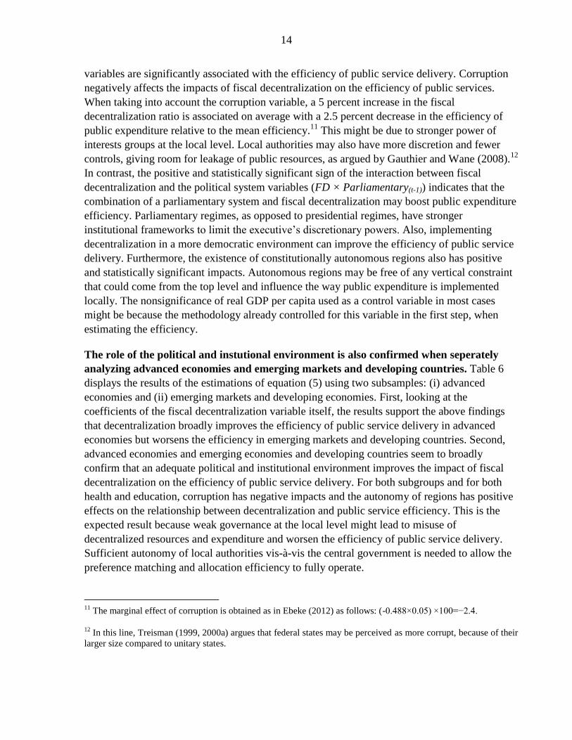
variables are significantly associated with the efficiency of public service delivery. Corruption
negatively affects the impacts of fiscal decentralization on the efficiency of public services.
When taking into account the corruption variable, a 5 percent increase in the fiscal
decentralization ratio is associated on average with a 2.5 percent decrease in the efficiency of
public expenditure relative to the mean efficiency.11
This might be due to stronger power of
interests groups at the local level. Local authorities may also have more discretion and fewer
controls, giving room for leakage of public resources, as argued by Gauthier and Wane (2008).12
In contrast, the positive and statistically significant sign of the interaction between fiscal
decentralization and the political system variables (FD × Parliamentary(t-1)) indicates that the
combination of a parliamentary system and fiscal decentralization may boost public expenditure
efficiency. Parliamentary regimes, as opposed to presidential regimes, have stronger
institutional frameworks to limit the executive’s discretionary powers. Also, implementing
decentralization in a more democratic environment can improve the efficiency of public service
delivery. Furthermore, the existence of constitutionally autonomous regions also has positive
and statistically significant impacts. Autonomous regions may be free of any vertical constraint
that could come from the top level and influence the way public expenditure is implemented
locally. The nonsignificance of real GDP per capita used as a control variable in most cases
might be because the methodology already controlled for this variable in the first step, when
estimating the efficiency.
The role of the political and instutional environment is also confirmed when seperately
analyzing advanced economies and emerging markets and developing countries. Table 6
displays the results of the estimations of equation (5) using two subsamples: (i) advanced
economies and (ii) emerging markets and developing economies. First, looking at the
coefficients of the fiscal decentralization variable itself, the results support the above findings
that decentralization broadly improves the efficiency of public service delivery in advanced
economies but worsens the efficiency in emerging markets and developing countries. Second,
advanced economies and emerging economies and developing countries seem to broadly
confirm that an adequate political and institutional environment improves the impact of fiscal
decentralization on the efficiency of public service delivery. For both subgroups and for both
health and education, corruption has negative impacts and the autonomy of regions has positive
effects on the relationship between decentralization and public service efficiency. This is the
expected result because weak governance at the local level might lead to misuse of
decentralized resources and expenditure and worsen the efficiency of public service delivery.
Sufficient autonomy of local authorities vis-à-vis the central government is needed to allow the
preference matching and allocation efficiency to fully operate.
11
The marginal effect of corruption is obtained as in Ebeke (2012) as follows: (-0.488×0.05) ×100=−2.4.
12 In this line, Treisman (1999, 2000a) argues that federal states may be perceived as more corrupt, because of their
larger size compared to unitary states.
15
Variables (1) (2) (3) (4) (5) (6) (7) (8)
FD(t-1) -0.523 -0.809 -1.307*** -0.727*** -1.079* -0.171 -0.764* -0.696
(-1.540) (-1.137) (-2.703) (-3.159) (-1.780) (-0.217) (-1.889) (-1.275)
FD × Corruption(t-1) -0.488*** -0.608***
(-3.291) (-2.738)
FD × Parliamentary(t-1) 4.373** 1.160
(2.206) (0.836)
FD × Regime(t-1) 0.033*** 0.0125
(2.967) (1.477)
FD × Autonomy(t-1) 2.057*** 1.952***
(5.457) (2.931)
Real GDP pc(t-1) -0.040 -0.122 -0.117*** 0.013 -0.130** -0.044 -0.0717** -0.020
(-1.535) (-1.598) (-2.803) (1.154) (-2.371) (-0.920) (-2.257) (-1.120)
Number of observations 810 875 874 875 639 690 689 690
Countries 51 55 55 55 49 53 53 53
Fisher (p-value ) 0.006 0.097 0.001 0.000 0.029 0.700 0.241 0.061
Hansen OID (p-value ) 0.408 0.868 0.422 0.139 0.900 0.012 0.004 0.141
KP-under 0.040 0.175 0.013 0.001 0.076 0.134 0.067 0.092
FD(t-1) instrumentation (p-value ) 0.000 0.000 0.000 0.000 0.038 0.229 0.014 0.047
FD × I (t-1) instrument. (p-value ) 0.058 0.226 0.000 0.000 0.161 0.115 0.000 0.000
Source: Authors’ calculations.
Health Education
Dependent variable: estimated efficiencies
Table 5. Fiscal Decentralization and Political/Institutional Environments
Note: (*), (**) and (***) denote statistical significance level of 10%, 5% and 1% percent respectively. Robust t-statistics in
parentheses.
Variables (1) (2) (3) (4) (5) (6) (7) (8)
FD(t-1) 0.106 0.874* -0.734*** -0.489*** 0.17 -1.255*** -1.455*** -0.975***
-0.264 -1.692 (-4.688) (-3.894) -0.392 (-2.614) (-4.384) (-2.864)
FD × Corruption(t-1) -0.274 -0.287*** -0.13 -0.470***
(-1.254) (-4.618) (-0.448) (-3.294)
FD × Autonomy(t-1) -0.264 1.344*** 1.754** 1.835***
(-0.509) -3.908 -2.54 -2.942
Real GDP pc(t-1) -0.108 0.013 0.002 0.017* -0.154 -0.064** -0.056* -0.010
(-1.146) -0.802 -0.147 -1.698 (-1.115) (-2.077) (-1.694) (-0.560)
Number of observations 266 269 544 606 211 213 428 477
Countries 14 14 37 41 14 14 35 39
Fisher (p-value ) 0.003 0.000 0.000 0.000 0.002 0.006 0.000 0.005
Hansen OID (p-value ) 0.472 0.036 0.400 0.002 0.228 0.404 0.922 0.101
KP-under 0.521 0.036 0.004 0.000 0.642 0.049 0.064 0.007
FD(t-1) instrumentation (p-value ) 0.000 0.000 0.000 0.000 0.000 0.000 0.027 0.018
FD × I (t-1) instrument. (p-value ) 0.171 0.000 0.002 0.000 0.538 0.002 0.050 0.000
Source: Authors’ calculations.
Note: (*), (**) and (***) denote statistical significance level of 10%, 5% and 1% percent respectively. Robust t-statistics in parentheses.
Table 6. Fiscal Decentralization and Political/Institutional Environments (sub-groups)
Dependent variable: estimated efficiencies
Health Education
Advanced EME and DC Advanced EME and DC
16
F. Robustness
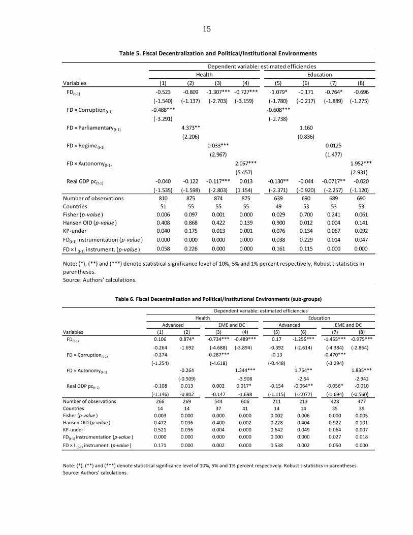
A range of sensitivity analysis is performed to assess the robustness of the findings.
Outliers are excluded from the baseline estimates. Then, the baseline model is reestimated using
a dependent variable—efficiency of public service delivery—that is derived through alternative
methodologies. Finally, the political and institutional variables are replaced with alternative
indicators.
The results are robust to the exclusion of countries with extreme ratios of fiscal
decentralization. The analysis is conducted using a narrowed sample. Countries totally or
almost totally centralized, i.e., with decentralization ratios close to zero, are excluded. Also,
countries that have extremely high degrees of decentralization, i.e., decentralization ratios
exceeding 90 percent, are dropped. A comparison of the results displayed in Table 7 with those
in Table 3 shows that the results are not driven by outliers. Regarding health, the impact of
decentralization remains positive for advanced economies, and negative for emerging markets
and developing economies, corroborating the baseline findings. The thrust of the results also
remains unchanged for education despite a slight difference in the magnitude of the coefficients.
The findings are robust to alternative methodologies of efficiency estimates. Two
methodologies are employed to compute alternative estimates of the efficiency of public service
delivery: a variante of stochastic frontier analysis based on Jondrow and others (1982) and a
methodology that takes into account the sample heterogeneity and heteroskedasticity. The
results shown in Table 8 focus on the role of political and institutional variables, and confirm
Advanced EME and DC Advanced EME and DC Advanced EME and DC Advanced EME and DC
Variables (1) (2) (3) (4) (5) (6) (7) (8)
FD(t-1) 0.599*** -0.338*** 0.599*** -0.388*** -0.0453 -0.884** -0.0453 -0.931**
-7.956 (-3.023) -7.956 (-3.315) (-0.339) (-2.560) (-0.339) (-2.410)
Real GDP pc(t-1) 0.00763 0.0224*** 0.00763 0.0134 -0.0767*** -0.00773 -0.0767*** -0.00673
(0.778) (2.627) (0.778) (1.426) (-4.339) (-0.437) (-4.339) (-0.341)
Number of observations 269 593 269 531 213 467 213 426
Countries 14 40 14 37 14 38 14 35
Fisher (p-value ) 0.000 0.000 0.000 0.000 0.000 0.039 0.000 0.056
Hansen OID (p-value ) 0.008 0.000 0.008 0.000 0.000 0.005 0.000 0.037
KP-under 0.000 0.000 0.000 0.000 0.002 0.056 0.002 0.061
FD(t-1) instrumentation (p-value ) 0.000 0.000 0.000 0.000 0.000 0.033 0.000 0.035
Note: (*), (**) and (***) denote statistical significance level of 10%, 5% and 1% percent respectively. Robust t-statistics in parentheses.
Source: Authors’ calculations.
0%<fd<90%
Table 7. Fiscal Descentralization and Public Expenditure Efficiency: Excluding Outliers
Health Education
Dependent variable: estimated efficiencies
Excluding outliers 0%<fd<90% Excluding outliers
17
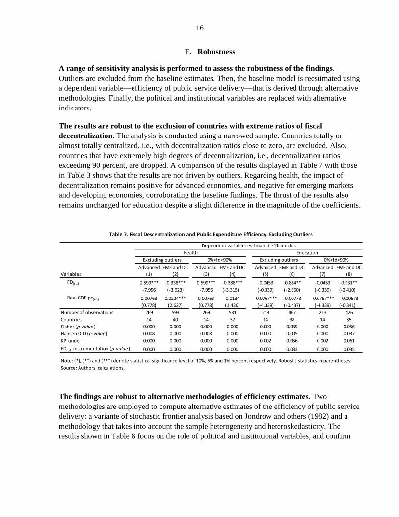
the findings from the baseline analysis.13 Under both alternative efficiency estimates, and for
both health and education, corruption hinders—with high statistical significance—the impacts
of fiscal decentralization on public service efficiency. The favorable role of parliamentary
regimes and more democratic institutions in combination with fiscal decentralization is also
confirmed, despite weak statistical significance in some cases. The positive impact of the
autonomy of regions on the relationship between fiscal decentralization and efficiency of public
service delivery is ascertained with high statistical significance in all cases (alternative
efficiency estimates and health and education).
The thrusts of the results remain unchanged under an approach that absorbs short-term
fluctuations. Fiscal decentralization changes slowly over time and plausibly affects the
efficiency of public services with time lags. Thus, it would be useful to check the robustness of
the results using averages of the variables over a few-year period. Accordingly, all variables are
averaged over a four-year period. In the efficiency of public service delivery and the fiscal
decentralization variables, the latter is introduced with a one-period lag. The results, displayed
in Table 9, support the baseline findings. Decentralization improves the efficiency of public
expenditure in advanced economies (columns 2 and 8). The impact seems negative for emerging
markets and developing countries, but it is not statistically significant. In terms of interactive
variables, the negative impact of corruption is confirmed (columns 4 and 10). The favorable
contribution of parliamentary regimes is also ascertained (columns 5 and 11). As for the
autonomy of regions, the impact is positive but not statistically significant.
Furthermore, the results are broadly robust to alternative political and institutional
variables. The following alternative variables are employed: bureaucracy, political stability,
and checks and balances.14 All those alternative variables lead to broadly similar inferences as
under the baseline analysis; the signs of the coefficiencts are mostly as expected, although
statistical significance is low in many cases (Table 10).
13
The pattern of nonlinearity is also broadly confirmed under the alternative efficiency estimates, but with lower
statistical significance.
14 The checks and balances variable measures the existence of effective control over the executive and legislative
branches in a presidential system. In parliamentary systems, checks and balances measure whether there is a one,
two, or three or more party coalition controlling the government.

18
Variables (1) (2) (3) (4) (5) (6) (7) (8) (9) (10) (11) (12) (13) (14) (15) (16)
FD(t-1) -0.560 -0.866 -1.392*** -0.781*** -0.488*** -0.389 -0.552*** -0.546*** -1.087* -0.174 -0.774* -0.702 -1.726** -0.694 -1.254** -1.327*
(-1.556) (-1.142) (-2.711) (-3.181) (-2.962) (-1.424) (-2.770) (-2.665) (-1.780) (-0.220) (-1.897) (-1.277) (-2.319) (-0.632) (-2.074) (-1.798)
FD × Corruption(t-1) -0.518*** -0.110** -0.612*** -0.778***
(-3.284) (-2.543) (-2.738) (-2.873)
FD × Parliamentary(t-1) 4.663** 0.979 1.161 1.777
(2.208) (1.508) (0.833) (0.872)
FD × Regime(t-1) 0.0355*** 0.009** 0.0126 0.0184
(2.970) (2.052) (1.477) (1.451)
FD × Autonomy(t-1) 2.199*** 1.069*** 1.965*** 3.121***
(5.504) (2.732) (2.939) (3.243)
Real GDP pc(t-1) -0.0415 -0.13 -0.125*** 0.0144 -0.099*** -0.112*** -0.132*** -0.084*** -0.131** -0.044 -0.072** -0.020 -0.089 0.023 -0.036 0.053**
(-1.516) (-1.596) (-2.825) (1.182) (-11.046) (-4.312) (-5.617) (-7.668) (-2.377) (-0.922) (-2.256) (-1.136) (-1.306) (0.322) (-0.732) (2.185)
Number of observations 810 875 874 875 719 778 777 778 639 690 689 690 639 690 689 690
Countries 51 55 55 55 51 55 55 55 49 53 53 53 49 53 53 53
Fisher (p-value ) 0.006 0.095 0.001 0.000 0.000 0.000 0.000 0.000 0.029 0.695 0.239 0.060 0.001 0.011 0.001 0.000
Hansen OID (p-value ) 0.398 0.871 0.437 0.136 0.009 0.154 0.085 0.246 0.901 0.012 0.004 0.141 0.722 0.028 0.033 0.425
KP-under 0.040 0.175 0.013 0.001 0.000 0.013 0.000 0.000 0.076 0.134 0.067 0.092 0.076 0.134 0.067 0.092
FD(t-1) instrumentation (p-value ) 0.000 0.000 0.000 0.000 0.000 0.000 0.000 0.000 0.038 0.229 0.014 0.047 0.038 0.229 0.014 0.047
FD × I (t-1) instrument. (p-value ) 0.058 0.226 0.000 0.000 0.000 0.039 0.000 0.000 0.161 0.116 0.000 0.000 0.161 0.116 0.000 0.000
Note: (*), (**) and (***) denote statistical significance level of 10%, 5% and 1% percent respectively. Robust t-statistics in parentheses.
Source: Authors’ calculations.
Table 8. Fiscal Decentralization and public expenditure efficiency: Alternative Efficiency Estimates
Dependent variables: Estimated efficiencies
Health Education
The Jondrow et al. (1982) approach Heterogeneous efficiencies The Jondrow et al. (1982) approach Heterogeneous efficiencies

19
All Advanced EME and DC All Advanced EME and DC
Variables (1) (2) (3) (4) (5) (6) (7) (8) (9) (10) (11) (12)
FD(t-1) -0.092 0.294*** -0.759 -0.350 -0.313 -1.637 -0.001 0.482*** -0.460 -0.550 -3.718 0.180
(-0.362) (3.091) (-1.514) (-1.198) (-0.512) (-1.506) (-0.001) (3.636) (-0.642) (-1.179) (-1.139) (0.136)
FD × Corruption(t-1) -0.136 -0.343***
(-1.539) (-2.654)
FD × Parliamentary(t-1) 1.977* 4.912
(1.689) (1.148)
FD × Autonomy(t-1) 1.455 0.0738
(1.607) (0.068)
Real GDP pc(t-1) 0.033*** 0.013 0.028 0.003 -0.049 0.020 -0.012 -0.124*** 0.007 -0.047 -0.155 -0.011
(3.484) (0.698) (1.400) (0.109) (-0.868) (0.832) (-0.414) (-3.991) (0.217) (-1.187) (-0.969) (-0.268)
Number of observations 221 63 158 203 221 221 199 61 138 184 199 199
Countries 55 14 41 51 55 55 52 14 38 48 52 52
Fisher (p-value ) 0.002 0.002 0.016 0.011 0.231 0.218 0.909 0.001 0.815 0.078 0.83 0.996
Hansen OID (p-value ) 0.012 0.219 0.318 0.422 0.674 0.691 0.065 0.059 0.045 0.267 0.899 0.087
KP-under 0.522 0.107 0.698 0.361 0.569 0.717 0.507 0.134 0.667 0.255 0.646 0.704
Note: (*), (**) and (***) denote statistical significance level of 10%, 5% and 1% percent respectively. Robust t-statistics in parentheses.
Source: Authors’ calculations.
Table 9: Fiscal Decentralization and Public Expenditure Efficiency: Absorbing Short-term Fluctuations
Dependent variables: 4-year average of estimated efficiencies
Health Education
Political interactions Political interactions
Variables (1) (2) (3) (4) (5) (6) (7) (8) (9) (10) (11) (12)
FD(t-1) -0.486* 0.953*** -0.597*** -1.408 -0.480*** -0.022 -0.007 0.786** -0.409 -0.811 0.565 -0.014
(-1.838) (3.609) (-3.131) (-1.513) (-2.741) (-0.061) (-0.003) (2.143) (-1.382) (-1.310) (1.519) (-0.008)
FD × Assembly elec.(t-1) 3.672*** 5.499
(3.093) (0.525)
FD × Presidential(t-1) -1.737*** -1.410***
(-4.999) (-2.583)
FD × All house(t-1) 0.541*** 0.13
(3.846) (1.452)
FD × Bureaucracy(t-1) 0.379 0.16
(0.953) (0.644)
FD × Political stab.(t-1) 0.102 0.459
(0.781) (1.394)
FD × Checks and balances(t-1) 0.141 -1.032
(0.924) (-1.216)
Real GDP pc(t-1) 0.054*** 0.002 0.004 -0.008 0.006 0.009 0.023 -0.034** -0.027*** -0.032 -0.022 0.080
(5.817) (0.169) (0.394) (-0.282) (0.412) (0.540) (0.786) (-2.319) (-2.715) (-1.541) (-1.065) (0.910)
Additional controls Yes Yes Yes Yes Yes Yes Yes Yes Yes Yes Yes Yes
Number of observations 875 875 844 807 602 868 690 690 664 639 482 684
Countries 55 55 54 51 55 55 53 53 51 49 51 53
Fisher (p-value ) 0.000 0.000 0.000 0.000 0.000 0.596 0.533 0.016 0.003 0.074 0.039 0.812
Hansen OID (p-value ) 0.009 0.631 0.001 0.003 0.000 0.012 0.598 0.011 0.000 0.002 0.094 0.483
KP-under 0.013 0.000 0.000 0.135 0.024 0.426 0.872 0.109 0.062 0.262 0.007 0.858
FD(t-1) instrumentation (p-value ) 0.000 0.000 0.000 0.000 0.004 0.000 0.302 0.024 0.034 0.057 0.045 0.075
FD × I (t-1) instrument. (p-value ) 0.042 0.000 0.000 0.002 0.141 0.622 0.263 0.228 0.000 0.385 0.059 0.938
Note: (*), (**) and (***) denote statistical significance level of 10%, 5% and 1% percent respectively. Robust t-statistics in parentheses.
Source: Authors’ calculations.
Health Education
Table 10: Fiscal Decentralization and Public Expenditure Efficiency: alternative political and institutional variables.
Dependent variable: estimated efficiencies
20
G. Revenue Decentralization
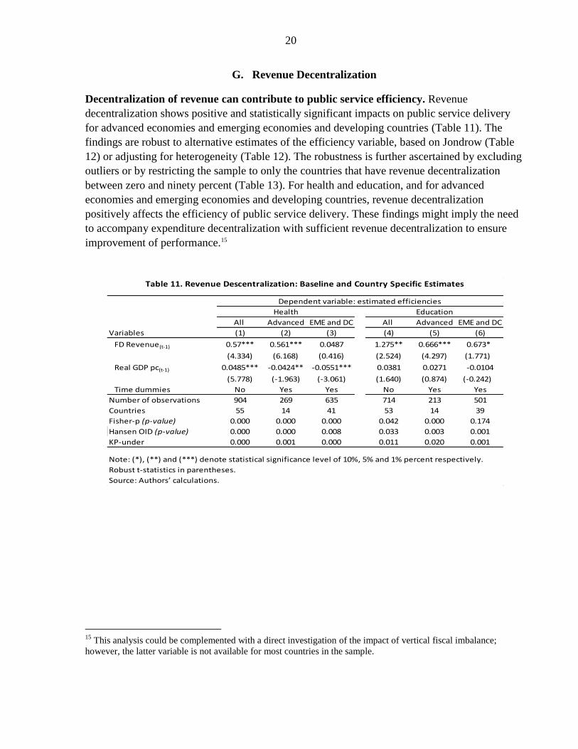
Decentralization of revenue can contribute to public service efficiency. Revenue
decentralization shows positive and statistically significant impacts on public service delivery
for advanced economies and emerging economies and developing countries (Table 11). The
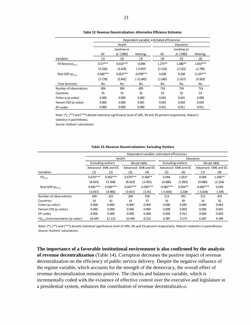
findings are robust to alternative estimates of the efficiency variable, based on Jondrow (Table
12) or adjusting for heterogeneity (Table 12). The robustness is further ascertained by excluding
outliers or by restricting the sample to only the countries that have revenue decentralization
between zero and ninety percent (Table 13). For health and education, and for advanced
economies and emerging economies and developing countries, revenue decentralization
positively affects the efficiency of public service delivery. These findings might imply the need
to accompany expenditure decentralization with sufficient revenue decentralization to ensure
improvement of performance.15
15
This analysis could be complemented with a direct investigation of the impact of vertical fiscal imbalance;
however, the latter variable is not available for most countries in the sample.
All Advanced EME and DC All Advanced EME and DC
Variables (1) (2) (3) (4) (5) (6)
FD Revenue(t-1) 0.57*** 0.561*** 0.0487 1.275** 0.666*** 0.673*
(4.334) (6.168) (0.416) (2.524) (4.297) (1.771)
Real GDP pc(t-1) 0.0485*** -0.0424** -0.0551*** 0.0381 0.0271 -0.0104
(5.778) (-1.963) (-3.061) (1.640) (0.874) (-0.242)
Time dummies No Yes Yes No Yes Yes
Number of observations 904 269 635 714 213 501
Countries 55 14 41 53 14 39
Fisher-p (p-value) 0.000 0.000 0.000 0.042 0.000 0.174
Hansen OID (p-value) 0.000 0.000 0.008 0.033 0.003 0.001
KP-under 0.000 0.001 0.000 0.011 0.020 0.001
Source: Authors’ calculations.
Note: (*), (**) and (***) denote statistical significance level of 10%, 5% and 1% percent respectively.
Robust t-statistics in parentheses.
Health Education
Table 11. Revenue Descentralization: Baseline and Country Specific Estimates
Dependent variable: estimated efficiencies
21
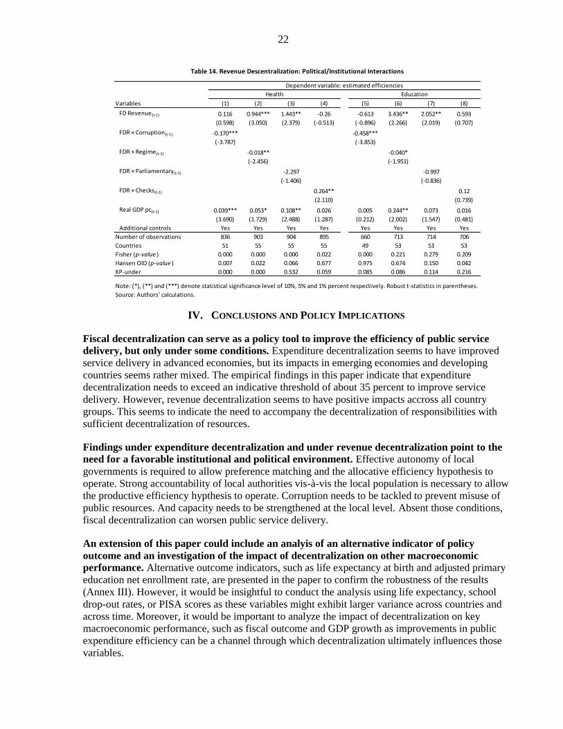
The importance of a favorable institutional environment is also confirmed by the analysis
of revenue decentralization (Table 14). Corruption decreases the positive impact of revenue
decentralization on the efficiency of public service delivery. Despite the negative influence of
the regime variable, which accounts for the strength of the democracy, the overall effect of
revenue decentralization remains positive. The checks and balances variable, which is
incrementally coded with the existence of effective control over the executive and legislature in
a presidential system, enhances the contribution of revenue decentralization.
All
Jondrow et
al. (1982) Heterog. All
Jondrow et
al. (1982) Heterog.
Variables (1) (2) (3) (4) (5) (6)
FD Revenue(t-1) 0.57*** 0.616*** -0.098 1.275** 1.286** 1.653***
(4.334) (4.429) (-0.997) (2.524) (2.532) (2.799)
Real GDP pc(t-1) 0.048*** 0.053*** -0.078*** 0.038 0.038 0.125***
(5.778) (5.842) (-12.645) (1.640) (1.627) (4.503)
Time dummies No No No No No No
Number of observations 904 904 805 714 714 714
Countries 55 55 55 53 53 53
Fisher-p (p-value) 0.000 0.000 0.000 0.042 0.041 0.000
Hansen OID (p-value) 0.000 0.000 0.001 0.033 0.034 0.029
KP-under 0.000 0.000 0.000 0.011 0.011 0.011
Source: Authors’ calculations.
Table 12: Revenue Decentralization: Alternative Efficiency Estimates
Health Education
Dependent variable: estimated efficiencies
Note: (*), (**) and (***) denote statistical significance level of 10%, 5% and 1% percent respectively. Robust t-
statistics in parentheses.
Advanced EME and DC Advanced EME and DC Advanced EME and DC Advanced EME and DC
Variables (1) (2) (3) (4) (5) (6) (7) (8)
FD(t-1) 0.670*** 0.463*** 0.670*** 0.366** 0.094 1.051* 0.094 1.036**
(8.023) (3.308) (8.023) (2.455) (0.680) (1.892) (0.680) (2.324)
Real GDP pc(t-1) 0.041*** 0.046*** 0.041*** 0.036*** -0.082*** 0.054** -0.082*** 0.039
(3.057) (4.983) (3.057) (3.35) (-5.654) -2.028 (-5.654) -1.595
Number of observations 269 622 269 528 213 491 213 423
Countries 14 41 14 37 14 39 14 35Fisher (p-value ) 0.000 0.000 0.000 0.004 0.000 0.081 0.000 0.063
Hansen OID (p-value ) 0.040 0.000 0.040 0.000 0.000 0.003 0.000 0.007
KP-under 0.000 0.000 0.000 0.000 0.004 0.012 0.004 0.003
FD(t-1) instrumentation (p-value ) 10.445 11.122 10.445 8.222 6.387 3.573 6.387 4.399
Source: Authors’ calculations.
Note: (*), (**) and (***) denote statistical significance level of 10%, 5% and 1% percent respectively. Robust t-statistics in parentheses.
Table 13: Revenue Decentralization: Excluding Outliers
Dependent variable: estimated efficiencies
Health Education
Excluding outliers 0%<fd <90% Excluding outliers 0%<fd <90%
22
IV. CONCLUSIONS AND POLICY IMPLICATIONS
Fiscal decentralization can serve as a policy tool to improve the efficiency of public service
delivery, but only under some conditions. Expenditure decentralization seems to have improved
service delivery in advanced economies, but its impacts in emerging economies and developing
countries seems rather mixed. The empirical findings in this paper indicate that expenditure
decentralization needs to exceed an indicative threshold of about 35 percent to improve service
delivery. However, revenue decentralization seems to have positive impacts accross all country
groups. This seems to indicate the need to accompany the decentralization of responsibilities with
sufficient decentralization of resources.
Findings under expenditure decentralization and under revenue decentralization point to the
need for a favorable institutional and political environment. Effective autonomy of local
governments is required to allow preference matching and the allocative efficiency hypothesis to
operate. Strong accountability of local authorities vis-à-vis the local population is necessary to allow
the productive efficiency hypthesis to operate. Corruption needs to be tackled to prevent misuse of
public resources. And capacity needs to be strengthened at the local level. Absent those conditions,
fiscal decentralization can worsen public service delivery.
An extension of this paper could include an analyis of an alternative indicator of policy
outcome and an investigation of the impact of decentralization on other macroeconomic
performance. Alternative outcome indicators, such as life expectancy at birth and adjusted primary
education net enrollment rate, are presented in the paper to confirm the robustness of the results
(Annex III). However, it would be insightful to conduct the analysis using life expectancy, school
drop-out rates, or PISA scores as these variables might exhibit larger variance across countries and
across time. Moreover, it would be important to analyze the impact of decentralization on key
macroeconomic performance, such as fiscal outcome and GDP growth as improvements in public
expenditure efficiency can be a channel through which decentralization ultimately influences those
variables.
Variables (1) (2) (3) (4) (5) (6) (7) (8)
FD Revenue(t-1) 0.116 0.944*** 1.443** -0.26 -0.613 3.436** 2.052** 0.593
(0.598) (3.050) (2.379) (-0.513) (-0.896) (2.266) (2.019) (0.707)
FDR × Corruption(t-1) -0.170*** -0.458***
(-3.787) (-3.853)
FDR × Regime(t-1) -0.018** -0.040*
(-2.456) (-1.951)
FDR × Parliamentary(t-1) -2.297 -0.997
(-1.406) (-0.836)
FDR × Checks(t-1) 0.264** 0.12
(2.110) (0.739)
Real GDP pc(t-1) 0.039*** 0.053* 0.108** 0.026 0.005 0.244** 0.073 0.016
(3.690) (1.729) (2.488) (1.287) (0.212) (2.002) (1.547) (0.481)
Additional controls Yes Yes Yes Yes Yes Yes Yes Yes
Number of observations 836 903 904 895 660 713 714 706
Countries 51 55 55 55 49 53 53 53
Fisher (p-value ) 0.000 0.000 0.000 0.022 0.000 0.221 0.279 0.209
Hansen OID (p-value ) 0.007 0.022 0.066 0.677 0.975 0.674 0.150 0.042
KP-under 0.000 0.000 0.532 0.059 0.085 0.086 0.114 0.216
Source: Authors’ calculations.
Health Education
Dependent variable: estimated efficiencies
Note: (*), (**) and (***) denote statistical significance level of 10%, 5% and 1% percent respectively. Robust t-statistics in parentheses.
Table 14. Revenue Descentralization: Political/Institutional Interactions
23
References
Ahmad, E., Brosio, G. and Tanzi, V. (2008) “Local Service Provision in Selected OECD
Countries: Do Decentralized Operations Work Better?”, IMF Working Paper 08/67.
Arze del Granado, F.A., Martinez-Vazquez, J. and McNab, R. (2005) "Fiscal Decentralization
and The Functional Composition of Public Expenditures", International Center for
Public Policy Working Paper Series.
Barankay, I. and Lockwood, B. (2007) "Decentralization and the Productive Efficiency of
Government: Evidence from Swiss Cantons", Journal of Public Economics, 91(5-6), pp.
1197-1218.
Bardhan, P. and Mukherjee, D. (2002) “Decentralization of Governance and Development”,
Journal of Economic Perspectives, pp. 185-205.
Battese G.E. and Coelli, T.J. (1988) “Prediction of Firm-level Technical Efficiencies: With a
Generalized Frontier Production Function and Panel Data”, Journal of Econometrics,
38, pp. 387-399.
Battese, G. E. and Coelli, T. J. (1995) “A Model for Technical Inefficiency Effects in a
Stochastic Frontier Production Function for Panel Data”, Empirical Economics, 20, pp.
325–332.
Bénassy-Quéré A., Gobalraja N. and Trannoy A. (2007) "Tax and Public Input Competition",
Economic Policy, CEPR & CES & MSH, 22(4), pp. 385-430.
Besley, T. and Smart, M. (2007) “Fiscal Restraints and Voter Welfare”, Journal of Public
Economics, 91, pp. 755–773.
Bordignon, M., Cerniglia, F., and Revelli, F. (2004) “Yardstick competition in
intergovernmental relationships: theory and empirical predictions”, Economics Letters,
83, pp. 325–333.
Cantarero, P.D. and Sanchez, M.P. (2006) “Decentralization and Health Care Outcomes: An
Empirical Analysis within the European Union”, Working Paper, University of
Cantabria, Spain.
Cornwell, C., Schmidt, P. and Sickles, R. (1990) "Production Frontiers with Cross Sectional
and Time Series Variation in Efficiency Levels", Journal of Econometrics, 46, pp. 185-
200.
Davoodi, H., Xie, D. and Zou, H. (1999) “Fiscal Decentralization and Economic Growth in the
United States”, Journal of Urban Economics 45, pp. 228-239.
24
Davoodi, H. and Zou, H. F. (1998) “Fiscal Decentralization and Economic Growth: A Cross-
country Study”, Journal of Urban Economics, 43(2), pp. 244-257.
Dziobek, C., Gutierrez-Mangas, C. and Kufa P. (2011) “Measuring Fiscal Decentralization –
Exploring the IMF’s Databases”, IMF Working Paper 11/126.
Ebeke, C. H. (2012) “The Power of Remittances on the International Prevalence of Child
Labor”, Structural Change and Economic Dynamics, 23(4), pp. 452–462.
Escolano, J., Eyraud, L., Moreno-Badia, M., Sarnes, J. and Tuladhar, A. (2012) “Fiscal
Performance, Institutional Design and Decentralization in European Union Countries”,
IMF Working Papers 12/45.
Ezcurra, R. and Rodríguez-Pose, A. (2010) "Does Decentralization Matter for Regional
Disparities? A Cross-country Analysis", Journal of Economic Geography, Oxford
University Press, 10(5), pp. 619-644.
Fredriksen, K. (2013) “Decentralization and Economic Growth-Part 3: Decentralization,
Infrastructure Investment and Educational Performance”, OECD Working Papers on
Fiscal Federalism, 16.
Gauthier, B. and Wane, W. (2007) "Leakage of Public Resources in the Health Sector: an
Empirical Investigation of Chad", Policy Research Working Paper Series, 4351.
Gonzalez-Alegre, J. (2010) "Decentralization and the Composition of Public Expenditure in
Spain", Regional Studies, 44(8), pp. 1067-1083.
Greene, W.H. (2005) “Efficiency of Public Spending in Developing Countries: A Stochastic
Frontier Approach,” World Bank.
Grigoli, F. (2014) “A Hybrid Approach to Estimating the Efficiency of Public Spending on
Education in Emerging and Developing Economies”, IMF Working Paper 14/19.
Grigoli, F. and Kapsoli, J. (2013) “Waste Not, Want Not: The Efficiency of Health Expenditure
in Emerging and Developing Economies”, IMF Working Papers 13/187.
Grisorio, M.J. and Prota, F. (2011) “The Impact of Fiscal Decentralization on the Composition
of Public Expenditure: Panel Data Evidence from Italy”, Societa italiana degli
economisti, 52.
25
Gupta, S. and Verhoeven, M. (2001) “The Efficiency of Government Expenditure. Experiences
from Africa” Journal of Policy Modelling, 23, pp. 433–467.
Gupta, S., Schwartz, G., Tareq, S., Allen, R., Adenauer, I., Fletcher, K. and Last D. (2007)
“Fiscal Management of Scale-Up Aid” IMF Working Paper No. 07/222.
Hayek, V. F. (1945) “The Use of Knowledge in Society”, American Economic Review, 35(4),
pp. 519-530.
Herrera, S. and Pang, G. (2005) “Efficiency of Public Spending in Developing Countries: An
Efficiency Frontier Approach” World Bank Policy Research Working Paper, 3645.
Hindriks, J. and Lockwood, B. (2005) “Decentralization and Electoral Accountability:
Incentives, Separation and Voter Welfare”, CEPR Discussion Paper, 5125.
Jayasuriya, R. and Wodon, Q. (2003) “Efficiency in Reaching the Millennium Development
Goals” World Bank Working Paper, 9.
Jiménez-Rubio, D. (2011) "The Impact of Fiscal Decentralization on Infant Mortality Rates:
Evidence from OECD Countries", Social Science & Medicine, 73(9), pp. 1401-1407.
Jondrow, J., Lovell, C.A.K., Materov, I.S. and Schmidt, P. (1982) "On the Estimation of
Technical Inefficiency in the Stochastic Frontier Production Function Model", Journal
of Econometrics, 19, pp. 233-238.
Kappeler, A. and Valila, T. (2008) "Fiscal Federalism and the Composition of Public
Investment in Europe”, European Journal of Political Economy, 24(3), pp. 562-570.
Kavosi, Z., Keshtkaran, A., Samadi, A.H. and Vahedi, S. (2013) “The Effect of Fiscal
Decentralization on Under-five Mortality in Iran: A Panel Data Analysis”, International
Journal of Health Policy and Management, 1(4), pp. 301-306.
Keen, M. and Marchand. M (1997) "Fiscal Competition and the Pattern of Public Spending"
Journal of Public Economics, Elsevier, 66(1), pp. 33-53.
Musgrave, R. (1969) “Theories of Fiscal Federalism”, Public Finance, 24(4), 521–32.
__________ (1999) “An Essay on Fiscal Federalism” Journal of Economic Literature.
Persson, T. and Tabellini, G. (2000) “Political Economics: Explaining Economic Policy”, MIT
Press, Cambridge, MA.
Phillips, K. and Woller, G.M. (1998) "Fiscal Decentralization and LDC Economic Growth: An
empirical Investigation", Journal of Development Studies, 34(4), pp. 139-148.
26
Redoano, M. (2003) “Does centralization affect the number and size of lobbies?”, CSGR
Discussion Paper, University of Warwick, 604.
Picazo, O. F., Robalino, D.A. and Voetberg, A. (2001) “Does Fiscal Decentralization Improve
Health Outcomes? Evidence from a cross-country analysis”, World Bank Policy
Research Working Paper, 2565.
Seabright, Paul. (1996) “Accountability and Decentralization in Government: An Incomplete
Contracts Model” European Economic Review, 40, pp. 61-89.
Ter-Minassian, T. (1997) “Decentralization and Macroeconomic Management”, IMF Working
Paper 97/155.
__________ (1997a) “Fiscal Federalism in Theory and Practice”, (Washington: International
Monetary Fund).
Thornton, J. (2007) "Fiscal Decentralization and Economic Growth Reconsidered", Journal of
Urban Economics, 61(1), pp. 64-70.
Tiebout, C.M. (1956) “A Pure Theory of Local Expenditures”, Journal of Political Economy, 64,
pp. 416-424.
Treisman, D. (1999a) “After the Deluge: Regional Crises and Political Consolidation in
Russia”, American Journal of Political Science.
____ (2000a) “The Causes of Corruption: A Cross-National Study”, Journal of Public
Economics.
Zhang, T. and Zou, H. (1998) "Fiscal Decentralization, Public Spending, and Economic Growth
in China", Journal of Public Economics, 67(2), pp. 221-240.
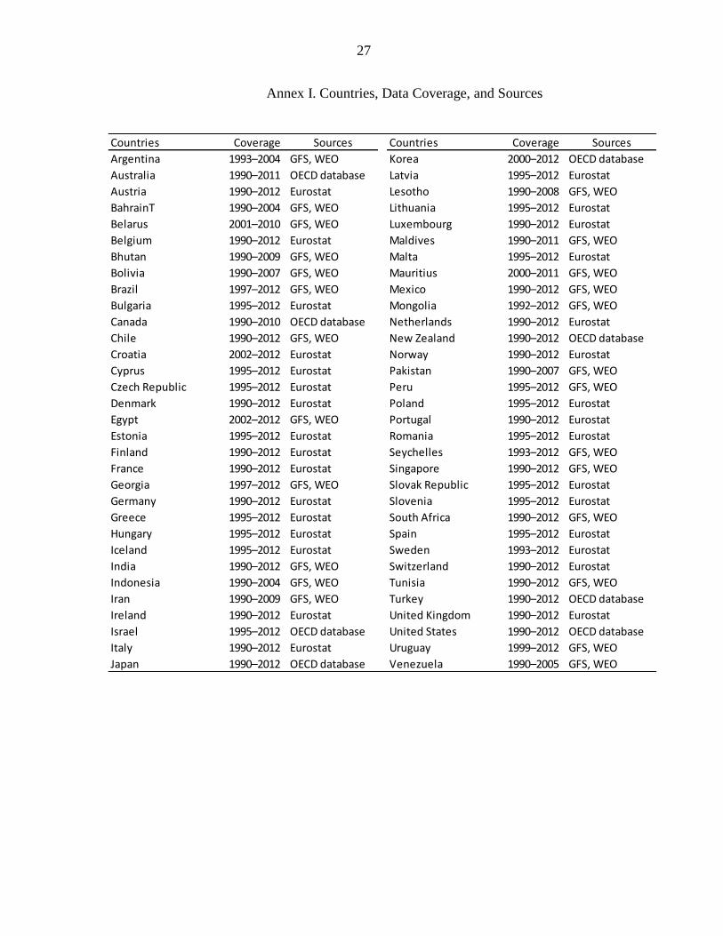
27
Annex I. Countries, Data Coverage, and Sources
Countries Coverage Sources Countries Coverage Sources
Argentina 1993–2004 GFS, WEO Korea 2000–2012 OECD database
Australia 1990–2011 OECD database Latvia 1995–2012 Eurostat
Austria 1990–2012 Eurostat Lesotho 1990–2008 GFS, WEO
BahrainT 1990–2004 GFS, WEO Lithuania 1995–2012 Eurostat
Belarus 2001–2010 GFS, WEO Luxembourg 1990–2012 Eurostat
Belgium 1990–2012 Eurostat Maldives 1990–2011 GFS, WEO
Bhutan 1990–2009 GFS, WEO Malta 1995–2012 Eurostat
Bolivia 1990–2007 GFS, WEO Mauritius 2000–2011 GFS, WEO
Brazil 1997–2012 GFS, WEO Mexico 1990–2012 GFS, WEO
Bulgaria 1995–2012 Eurostat Mongolia 1992–2012 GFS, WEO
Canada 1990–2010 OECD database Netherlands 1990–2012 Eurostat
Chile 1990–2012 GFS, WEO New Zealand 1990–2012 OECD database
Croatia 2002–2012 Eurostat Norway 1990–2012 Eurostat
Cyprus 1995–2012 Eurostat Pakistan 1990–2007 GFS, WEO
Czech Republic 1995–2012 Eurostat Peru 1995–2012 GFS, WEO
Denmark 1990–2012 Eurostat Poland 1995–2012 Eurostat
Egypt 2002–2012 GFS, WEO Portugal 1990–2012 Eurostat
Estonia 1995–2012 Eurostat Romania 1995–2012 Eurostat
Finland 1990–2012 Eurostat Seychelles 1993–2012 GFS, WEO
France 1990–2012 Eurostat Singapore 1990–2012 GFS, WEO
Georgia 1997–2012 GFS, WEO Slovak Republic 1995–2012 Eurostat
Germany 1990–2012 Eurostat Slovenia 1995–2012 Eurostat
Greece 1995–2012 Eurostat South Africa 1990–2012 GFS, WEO
Hungary 1995–2012 Eurostat Spain 1995–2012 Eurostat
Iceland 1995–2012 Eurostat Sweden 1993–2012 Eurostat
India 1990–2012 GFS, WEO Switzerland 1990–2012 Eurostat
Indonesia 1990–2004 GFS, WEO Tunisia 1990–2012 GFS, WEO
Iran 1990–2009 GFS, WEO Turkey 1990–2012 OECD database
Ireland 1990–2012 Eurostat United Kingdom 1990–2012 Eurostat
Israel 1995–2012 OECD database United States 1990–2012 OECD database
Italy 1990–2012 Eurostat Uruguay 1999–2012 GFS, WEO
Japan 1990–2012 OECD database Venezuela 1990–2005 GFS, WEO

28
Annex II. Variables, Definitions and Data Sources
Variables Description Sources
Fiscal variables
Expenditure decentralization Fiscal decentralization - Expenditures side
Revenue decentralization Fiscal decentralization - Revenue side
Demographic and macro variables
Imr Mortality rate, infant (per 1,000 live births)
Umr Mortality rate, under-5 (per 1,000 live births)
Primary education Primary education, duration (years)
Secondary education Secondary education, duration (years)
Average year of schooling Average year of primary and secondary schooling
Total population Measures the size of the population
Density Population density (people per sq. km of land area)
Real GDP pc GDP per capita, PPP (constant 2011 international)
Natural ressources (% GDP) Natural resource rents
Health and education variables
Health expenditure Health expenditure, public (% of GDP)
Primary enrollment Gross enrollment ratio, primary, both sexes (%)
Secondary enrollment Gross enrollment ratio, secondary, both sexes (%)
Education exp. Government expenditure on education as % of GDP (%)
Political and institutional variables
Polstab Political stability measures the likelihood that the
government will be destabilized by unconstitutional or
violent means.
The WGI, 2013 Update
Government fractionalization Probability that two deputies randomly picked from the
government parties will be of different parties.
Fractionalization The probability that two deputies picked from the
legislature will be of different parties.
Parliamentary Dummy variable that takes value 1 if the political system
is parliamentary
Democracy Variable recording the strenght of the democracy
Autonomy Dummy variable taking value 1 with the existence of
autonomous region
Corruption Assessment of corruption within the political system. ICRG database
Eurostat, GFS, OECD
and WEO
World Bank, World
Development
Indicators 2014
OECD and UNESCO
databases
DPI2012 Database of
Political Institutions:
Note: Expenditure and Revenue descentralization for European and OECD countries are taken respectively from
Eurostat and OECD databases. For emerging economies and developing countries, data are from GFS and WEO.
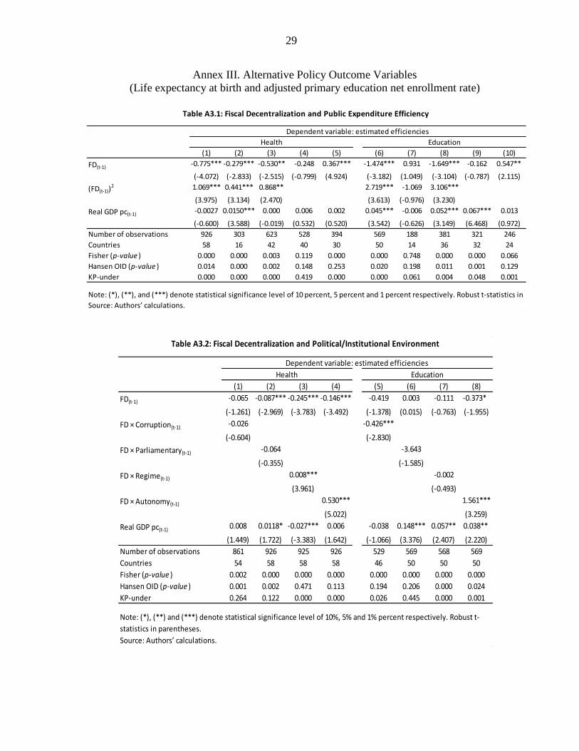
29
Annex III. Alternative Policy Outcome Variables
(Life expectancy at birth and adjusted primary education net enrollment rate)
(1) (2) (3) (4) (5) (6) (7) (8) (9) (10)
FD(t-1) -0.775*** -0.279*** -0.530** -0.248 0.367*** -1.474*** 0.931 -1.649*** -0.162 0.547**
(-4.072) (-2.833) (-2.515) (-0.799) (4.924) (-3.182) (1.049) (-3.104) (-0.787) (2.115)
(FD(t-1))2 1.069*** 0.441*** 0.868** 2.719*** -1.069 3.106***
(3.975) (3.134) (2.470) (3.613) (-0.976) (3.230)
Real GDP pc(t-1)-0.0027 0.0150*** 0.000 0.006 0.002 0.045*** -0.006 0.052*** 0.067*** 0.013
(-0.600) (3.588) (-0.019) (0.532) (0.520) (3.542) (-0.626) (3.149) (6.468) (0.972)
Number of observations 926 303 623 528 394 569 188 381 321 246
Countries 58 16 42 40 30 50 14 36 32 24
Fisher (p-value ) 0.000 0.000 0.003 0.119 0.000 0.000 0.748 0.000 0.000 0.066
Hansen OID (p-value ) 0.014 0.000 0.002 0.148 0.253 0.020 0.198 0.011 0.001 0.129
KP-under 0.000 0.000 0.000 0.419 0.000 0.000 0.061 0.004 0.048 0.001
Source: Authors’ calculations.
Table A3.1: Fiscal Decentralization and Public Expenditure Efficiency
Health Education
Dependent variable: estimated efficiencies
Note: (*), (**), and (***) denote statistical significance level of 10 percent, 5 percent and 1 percent respectively. Robust t-statistics in
(1) (2) (3) (4) (5) (6) (7) (8)
FD(t-1) -0.065 -0.087*** -0.245*** -0.146*** -0.419 0.003 -0.111 -0.373*
(-1.261) (-2.969) (-3.783) (-3.492) (-1.378) (0.015) (-0.763) (-1.955)
FD × Corruption(t-1) -0.026 -0.426***
(-0.604) (-2.830)
FD × Parliamentary(t-1) -0.064 -3.643
(-0.355) (-1.585)
FD × Regime(t-1) 0.008*** -0.002
(3.961) (-0.493)
FD × Autonomy(t-1) 0.530*** 1.561***
(5.022) (3.259)
Real GDP pc(t-1)0.008 0.0118* -0.027*** 0.006 -0.038 0.148*** 0.057** 0.038**
(1.449) (1.722) (-3.383) (1.642) (-1.066) (3.376) (2.407) (2.220)
Number of observations 861 926 925 926 529 569 568 569
Countries 54 58 58 58 46 50 50 50
Fisher (p-value ) 0.002 0.000 0.000 0.000 0.000 0.000 0.000 0.000
Hansen OID (p-value ) 0.001 0.002 0.471 0.113 0.194 0.206 0.000 0.024
KP-under 0.264 0.122 0.000 0.000 0.026 0.445 0.000 0.001
Source: Authors’ calculations.
Health Education
Table A3.2: Fiscal Decentralization and Political/Institutional Environment
Dependent variable: estimated efficiencies
Note: (*), (**) and (***) denote statistical significance level of 10%, 5% and 1% percent respectively. Robust t-
statistics in parentheses.
Top Related