


Languages
Pages
Legal


Bank of Canada Banque du Canada
Working Paper 2004-22 / Document de travail 2004-22
Financial Conditions Indexes for Canada
by
Céline Gauthier, Christopher Graham, and Ying Liu

ISSN 1192-5434
Printed in Canada on recycled paper

Bank of Canada Working Paper 2004-22
June 2004
Financial Conditions Indexes for Canada
by
Céline Gauthier, 1 Christopher Graham, 2 and Ying Liu 1
1Monetary and Financial Analysis DepartmentBank of Canada
Ottawa, Ontario, Canada K1A [email protected]
2 International DepartmentBank of Canada
Ottawa, Ontario, Canada K1A [email protected]
The views expressed in this paper are those of the authors.No responsibility for them should be attributed to the Bank of Canada.


iii
Contents
Acknowledgements. . . . . . . . . . . . . . . . . . . . . . . . . . . . . . . . . . . . . . . . . . . . . . . . . . . . . . . . . . . . ivAbstract/Résumé. . . . . . . . . . . . . . . . . . . . . . . . . . . . . . . . . . . . . . . . . . . . . . . . . . . . . . . . . . . . . . . v
1. Introduction . . . . . . . . . . . . . . . . . . . . . . . . . . . . . . . . . . . . . . . . . . . . . . . . . . . . . . . . . . . . . . 1
2. The Literature on FCIs. . . . . . . . . . . . . . . . . . . . . . . . . . . . . . . . . . . . . . . . . . . . . . . . . . . . . . 4
2.1 Variables included in an FCI . . . . . . . . . . . . . . . . . . . . . . . . . . . . . . . . . . . . . . . . . . . . 4
2.2 Detrending the variables . . . . . . . . . . . . . . . . . . . . . . . . . . . . . . . . . . . . . . . . . . . . . . . . 5
2.3 Weighting the variables . . . . . . . . . . . . . . . . . . . . . . . . . . . . . . . . . . . . . . . . . . . . . . . . 6
2.4 FCIs as tools . . . . . . . . . . . . . . . . . . . . . . . . . . . . . . . . . . . . . . . . . . . . . . . . . . . . . . . . . 7
2.5 Criticisms of FCIs. . . . . . . . . . . . . . . . . . . . . . . . . . . . . . . . . . . . . . . . . . . . . . . . . . . . . 8
3. Three Ways to Derive an FCI for Canada . . . . . . . . . . . . . . . . . . . . . . . . . . . . . . . . . . . . . . . 9
3.1 FCIs based on a reduced-form model . . . . . . . . . . . . . . . . . . . . . . . . . . . . . . . . . . . . . . 9
3.2 FCIs based on generalized impulse-response functions . . . . . . . . . . . . . . . . . . . . . . . 11
3.3 FCIs based on factor analysis . . . . . . . . . . . . . . . . . . . . . . . . . . . . . . . . . . . . . . . . . . . 13
4. Properties of Our FCIs. . . . . . . . . . . . . . . . . . . . . . . . . . . . . . . . . . . . . . . . . . . . . . . . . . . . . 14
4.1 FCIs based on a reduced-form model . . . . . . . . . . . . . . . . . . . . . . . . . . . . . . . . . . . . . 15
4.2 FCIs based on generalized impulse-response functions . . . . . . . . . . . . . . . . . . . . . . . 19
4.3 FCIs based on factor analysis . . . . . . . . . . . . . . . . . . . . . . . . . . . . . . . . . . . . . . . . . . . 20
4.4 Comparison of our FCIs . . . . . . . . . . . . . . . . . . . . . . . . . . . . . . . . . . . . . . . . . . . . . . . 21
5. Comparing the IS-Curve-Based FCI with the MCI . . . . . . . . . . . . . . . . . . . . . . . . . . . . . . . 22
6. Interpreting the FCI as a Measure of Financial Stance . . . . . . . . . . . . . . . . . . . . . . . . . . . . 23
7. Conclusion . . . . . . . . . . . . . . . . . . . . . . . . . . . . . . . . . . . . . . . . . . . . . . . . . . . . . . . . . . . . . . 24
Bibliography . . . . . . . . . . . . . . . . . . . . . . . . . . . . . . . . . . . . . . . . . . . . . . . . . . . . . . . . . . . . . . . . . 26
Tables . . . . . . . . . . . . . . . . . . . . . . . . . . . . . . . . . . . . . . . . . . . . . . . . . . . . . . . . . . . . . . . . . . . . . . 29
Figures. . . . . . . . . . . . . . . . . . . . . . . . . . . . . . . . . . . . . . . . . . . . . . . . . . . . . . . . . . . . . . . . . . . . . . 37

iv
Acknowledgements
This paper has benefited from the useful comments of Pierre St-Amant, Jean-Paul Lam, Jackson
Loi, Virginie Traclet, Carolyn Wilkins, and participants at two Bank of Canada workshops. We
thank Marc-André Gosselin and Greg Tkacz for sharing their RATS codes for the factor analysis,
and Lingyun Xue for research assistance. All remaining errors are our own.

v
r
ditions
cal
in-
ing
risk
ificant
f
ier est
et le
es
étaires
alués à
, leur
ique
la
de
latives
nt
étaires
Abstract
The authors construct three financial conditions indexes (FCIs) for Canada based on three
approaches: an IS-curve-based model, generalized impulse-response functions, and facto
analysis. Each approach is intended to address one or more criticisms of the monetary con
index (MCI) and existing FCIs. To evaluate their three FCIs, the authors consider five
performance criteria: the consistency of each FCI’s weight with economic theory, its graphi
ability to predict turning points in the business cycle, its dynamic correlation with output, its
sample fit in explaining output, and its out-of-sample performance in forecasting output. Us
monthly data, the authors find, in general, that housing prices, equity prices, and bond yield
premiums, in addition to short- and long-term interest rates and the exchange rate, are sign
in explaining output from 1981 to 2000. They also find that the FCIs outperform the Bank o
Canada’s MCI in many areas.
JEL classification: E44, E52Bank classification: Monetary and financial indicators; Monetary conditions index
Résumé
Les auteurs élaborent trois nouveaux indices des conditions financières au Canada. Le prem
fondé sur la courbe IS, le second sur l’établissement de courbes de réaction généralisées
troisième sur l’analyse factorielle. Les méthodes retenues pour la construction de ces indic
visent à répondre à l’un ou plusieurs des reproches adressés à l’indice des conditions mon
de la Banque du Canada et aux autres indices en usage. Les trois nouveaux indices sont év
l’aune des cinq critères suivants : la conformité de leur pondération à la théorie économique
capacité à prévoir les points de retournement du cycle économique, leur corrélation dynam
avec la production, leur capacité à expliquer la production à l’intérieur de l’échantillon et à
prévoir hors échantillon. Travaillant avec des données mensuelles, les auteurs constatent,
manière générale, que le prix des logements, les cours boursiers et les primes de risque re
aux obligations, tout comme les taux d’intérêt à court et à long terme et le taux de change,
permettent d’expliquer l’évolution que la production a connue entre 1981 et 2000. Ils relève
également que leurs indices surpassent, à de nombreux égards, l’indice des conditions mon
de la Banque.
Classification JEL : E44, E52Classification de la Banque : Indicateurs monétaires et financiers; Indice des conditionsmonétaires


1
equity
ect
fect
o a
itional
en
t role
ck
tock
at
-7
rices
an the
possess
mine
ection
ely,
ns,
n
the
hich
aas
1. Introduction
The transmission of monetary policy has traditionally been explained using an interest rate
channel and an exchange rate channel. Some research, however, implies that property and
prices may also play an important role in the transmission mechanism through a wealth eff
(e.g., Modigliani 1971) and a credit channel (e.g., Bernanke and Gertler 1989). A wealth ef
occurs when a change in asset prices affects the financial wealth of individuals and leads t
change in their consumption decisions. A credit channel exists when a rise in asset prices
increases the borrowing capacity of individuals and firms by expanding the value of their
collateral. This increase in available credit allows households and businesses to make add
purchases of goods and services and, therefore, boost aggregate demand.
The usefulness of asset prices in determining aggregate demand and inflation has long be
controversial. Although, from a theroretical viewpoint, asset prices seem to play a significan
in the transmission mechanism, the empirical evidence is mixed. Many studies find that sto
returns possess little predictive content for future output (e.g., Fama 1981; Harvey 1989; S
and Watson 1989, 1999; Estrella and Mishkin 1998). Goodhart and Hofmann (2000) find th
stock prices have no marginal predictive content for inflation in their international data set of
seventeen developed countries. Using a backward-looking IS-Phillips curve model for the G
countries, however, Goodhart and Hofmann (2001) suggest that both housing and share p
have a significant impact on theoutput gap. They also find that the effect of housing prices is
larger than that of stock prices and, in most cases—including that of Canada—also larger th
effect of the exchange rate.1
Research at the Bank of Canada suggests that asset prices, especially property prices, may
important information about future inflationary pressure. Pichette and Tremblay (2003) exa
the link between consumption and disaggregate wealth in Canada. Using a vector-error-corr
model, the authors find evidence of a significant housing wealth effect for Canada. Convers
the evidence regarding the stock market wealth effect is weak. In terms of policy implicatio
other things being equal, Pichette and Tremblay suggest that more weight should be put o
fluctuations in housing prices than on fluctuations in stock prices. On the other hand, using
same methodology to examine the links between financial markets and the real economy,
Gauthier and Li (2004) find that real stock prices and output are cointegrated one for one, w
1. Because Goodhart and Hofmann obtain similar weights when using the impulse responses fromstructural vector autoregression (VAR), these weights can be considered to be structural as longtheir identification assumptions are considered reasonable.

2
t
ve
t the
er cent,
only
rform
S&P)
to be
prices,
nism.
r a
ly
the
ny
sition
authors
nce.
asures
sures
ding to
e
nd
ly
suggests that stock price movements at low frequency are closely linked to potential outpu
changes.
In another Bank of Canada study, Zhang (2002) suggests that bond risk premiums may ha
strong predictive power for future output. Using U.S. data from 1988 to 2001, Zhang finds tha
high-yield bond spread and the investment-grade spread can explain 68 per cent and 42 p
respectively, of employment variations one year ahead, while the term spread can explain
12 per cent. For output forecasts up to one year ahead, corporate bond spreads also outpe
popular indicators such as the commercial paper–treasury bill spread, federal funds rate,
consumer sentiment index, Conference Board leading indicator, and the Standard & Poor’s (
index both in-sample and out-of-sample. The forecasts from the high-yield spread are found
more accurate than those from the investment-grade spreads.
The composition of Canadian household total assets (Table 1) also suggests that housing
equity prices, and relative bond yields may play an important role in the transmission mecha
Property assets account for a third of total household assets in Canada. Stocks account fo
significant portion (more than 10 per cent) of total assets and their importance has gradual
increased over the past 20 years. While the direct holding of bonds has decreased slightly,
importance of life insurance and pensions has risen significantly. This suggests that so ma
households hold more bonds indirectly through an investment vehicle that the actual compo
of bonds in the investment vehicle portfolio may have in fact increased.2
In an attempt to capture these possible effects of asset prices on the real economy, several
and institutions include them when they construct new measures of the monetary policy sta
These measures, often called financial conditions indexes (FCIs), expand on traditional me
of policy stance by including other indicators of the tightness of financial conditions that
economic agents face and that are affected by monetary policy. FCIs normally contain mea
of interest rates, exchange rates, and housing and equity market conditions, weighted accor
an economic model. Studies show that these indexes generally outperform the traditional
monetary conditions index (MCI), a weighted average of the short-term interest rate and th
exchange rate, in tracing and predicting output and inflation (see, for example, Goodhart a
Hofmann 2002, Lack 2002).3 Nevertheless, FCIs still suffer from certain criticisms that also app
to the MCI, such asmodel dependency, ignored dynamics, parameter inconstancy, andnon-
exogeneity of regressors(see, for example, Eika, Ericsson, and Nymoen 1996; Ericsson et al.
1998).
2. The wealth effect from an increase in the value of an insurance policy or a pension plan onconsumption may not be significant.
3. Section 5 provides a more detailed comparison between the MCI and our FCIs.

3
d on
dress
he
t of
ded by
s
out-
rly
ential
em of
the
st
ificant
ond
d. Out
d
tput
t-
I that
CIs
ture
cusses
ank’s
nd
In this paper, we review these existing indexes and propose several FCIs for Canada base
different approaches. Our contribution to the literature is that each approach is intended to ad
one or more criticisms of the MCI and existing FCIs. Our first approach derives component
weights from an IS-Phillips curve framework in two ways: using the sum of coefficients on t
lags of variables, and including individual lags in the FCI to take into account thedynamics of
variables over time. Our second and third approaches focus on the criticism ofnon-exogeneity of
regressors andmodel dependency, deriving weights based on generalized impulse-response
functions from a VAR and factor analysis. For all three methods, we experiment with one se
variables detrended with a Hodrick and Prescott (HP) (1980) filter and a second set detren
first-differencing. We then evaluate our different FCIs according to the consistency of their
weights with economic theory, their graphical ability to predict turning points in the busines
cycle, their dynamic correlation with output, their in-sample fit in explaining output, and their
of-sample performance in forecasting output. Although it is common practice to use quarte
data starting from the 1960s, we use monthly data from 1981 to 2000. We thereby avoid pot
structural breaks caused by the oil-price shocks of the 1970s, and partly address the probl
parameter inconstancy. Furthermore, the higher data frequency is more analytically useful for
Bank’s yearly fixed schedule of eight dates for announcing decisions on its key policy intere
rate.
Based on the IS-curve method, we find that housing prices, equity prices, and bond risk
premiums, in addition to short- and long-term interest rates and the exchange rate, are sign
in explaining output from 1981 to 2000. We also find that our FCIs that use a U.S. high-yield b
spread perform better than our FCIs that include a Canadian investment-grade bond sprea
of the eight FCIs that are based on all three approaches, two have particularly well-rounde
attributes, according to our criteria. The best short-term (less than one year) predictor of ou
growth is the FCI that derives its weights from summed coefficients of an IS curve using firs
differenced data; the best longer-term (one to two years) predictor of output growth is the FC
derives its weights from VAR impulse-response functions using first-differenced data. Our F
also largely outperform the MCI in many criteria considered in this paper.
The rest of this paper is organized as follows. Section 2 provides a critical review of the litera
on FCIs. Section 3 describes the three approaches we use to construct FCIs. Section 4 dis
the properties and performance of our FCIs. Section 5 compares the IS-based FCI with the B
MCI. Section 6 discusses the interpretation of our FCIs as a measure of financial stance, a
section 7 concludes with suggestions for future research.

4
ing
which
bles
te is
e
me
inder
ich the
term
levant
hs and
at the
a, the
d
hile
n, the
hold
the
into
the
ns
Mayes
ictive
f
2. The Literature on FCIs
Researchers from central banks and various private organizations have developed FCIs to
complement existing measures of policy stance. Table 2 summarizes the variables, detrend
methods, and weighting schemes used in these FCIs.
2.1 Variables included in an FCI
All FCIs, so far as we can ascertain, include a short-term interest rate and an exchange rate,
implies that all FCIs are extensions of the MCI. As Freedman (1995) illustrates, the two varia
contain important information about the stance of monetary policy. The short-term interest ra
sometimes considered a measure of this stance in itself, since it is highly correlated with th
policy instrument—the overnight rate—and has been found in numerous studies to bear so
predictive power for output and inflation (see, for example, Sims 1980 and Bernanke and Bl
1992). The inclusion of the exchange rate captures the exchange rate channel, through wh
relative price of imports and exports affects aggregate demand. This channel is particularly
important for a small open economy like Canada.
Some FCIs include a long-term interest rate or a corporate bond risk premium. While long-
rates are affected less directly by monetary policy than the short-term rate, they are more re
to the financing decisions of businesses and households. It is interesting that Goldman Sac
J.P. Morgan include the term spread in their FCI for Canada. While many studies suggest th
term spread has more predictive power for inflation than the short-term interest rate in Canad
use of both these variables may imply overlapping information (see, for example, Cozier an
Tkacz 1994).
Existing FCIs differ most in the variables they use to represent equity market conditions. W
stock prices are most intuitive, some private institutions also use measures of stock valuatio
equity market capitalization-to-GDP ratio, the dividend price ratio, and a measure of house
equity wealth. Macroeconomic Advisers (1998) reports that the idea behind their choice of
dividend-price ratio and household equity wealth is that the wealth channel can be divided
two parts: that which affects households directly, and that which affects businesses through
equity cost of capital. Apart from that, there is insufficient information on how other institutio
in Table 2 chose their particular measures of stock market conditions over alternatives.
Property prices are used in the FCIs of Goodhart and Hofmann (2001) and, subsequently,
and Virén (2001). Both studies find that property prices have stronger explanatory and pred
power for inflation than do equity prices. Goodhart and Hofmann also find that the impact o
5
r, they
ses of
en so
t the
ables
ity in
e
ng the
n
lies
ses
se
y-
rium
s
me
e rate
rying
02).s.
housing prices on the output gap is larger than that of the exchange rate in Canada. Howeve
acknowledge that the timeliness of data on housing prices remains a challenge for the purpo
an FCI.
In Table 2, only J.P. Morgan’s FCI includes monetary aggregates. The variables were chos
that the index includes “monetary and financial indicators that the Bank of Canada has
emphasized at various times in the past [or] well known financial market indicators that reflec
cost of funds to Canadian businesses.”4
2.2 Detrending the variables
Detrending of variables is an important issue because it is directly related to the way the vari
are modelled and the FCI interpreted. Detrending is mainly used to deal with non-stationar
many economic series for the purpose of econometric modelling. Depending on whether th
series has a stochastic trend or a deterministic trend, first-differencing the variables and taki
deviation from a linear trend can be applied, respectively. A time-varying trend or a deviatio
from an estimated equilibrium value can also be used.
The HP filter is a popular method of deriving a time-varying trend. Despite its simplicity,
however, the filter is subject to some criticism, particularly that it is two-sided. This fact imp
that the calculated trend in a given period depends on data from the next period, which cau
practical problems when generating timely analysis and forecasts.5 One way to reduce this
problem would be to complete the observed data with mechanical projections, such as tho
obtained from a univariate process.
An advantage of deriving a long-run trend, or equilibrium value, for all the variables is that a
positive deviation of the FCI from its equilibrium value can be interpreted as a relatively
accommodative stance, and vice versa. This interpretation is particularly important if a polic
maker wants to use the FCI as an operational target. However, finding a time-varying equilib
value for these variables, as for any other economic variable, is difficult and usually involve
extensive modelling work.
Goodhart and Hofmann (2001) define all four of their chosen variables in deviation from so
trend. The “trend” for the short-term interest rate is its sample mean and that of the exchang
and housing prices is their linear trend. In the case of equity prices, because of the time-va
nature of the expectations for future dividend growth, an HP filter with a high smoothing
4. This quotation is taken from correspondence with Ted Carmichael, of J.P. Morgan (25 March 205. See Guay and St-Amant (1996) for a more detailed explanation of the HP filter and its drawback

6
e
bles of
ough
is:
to
uced-
and
ality,
ensus
mand
e as a
est
output
in the
gy is
lead to
that
an
d based
g 12
ons
ll
parameter of 10,000 is used. The deviation of each variable from its trend is then used in th
construction of the index.6
2.3 Weighting the variables
In the literature, two main methods are used to determine and weight the component varia
an FCI. The first is to try to explain the role of asset prices in the transmission mechanism thr
economic modelling. As Goodhart and Hofmann (2000) state, there are three ways to do th
• simulation in a large-scale macroeconometric model• reduced-form aggregate-demand equations• VAR impulse-response functions
Large-scale models are designed to capture structural features of the economy and take in
account the interaction of all variables. Therefore, they might be more appropriate than red
form aggregate-demand equations and VAR impulse-response functions. Goldman Sachs
Macroeconomic Advisers use this approach to construct an FCI for the United States. In re
however, stock and other asset prices play a limited role in many large-scale macro models
currently used by central banks and other organizations. This is partly due to the lack of cons
in the theoretical literature on the channels through which asset prices affect aggregate de
and inflation. As a result, reduced-form equations and VAR impulse-response functions serv
useful alternative to estimate such an effect from empirical data.
A typical reduced-form model consists of an IS equation that relates the output gap to inter
rates, exchange rates, and other asset prices, and a Phillips curve that relates inflation to the
gap. Generally, the choice of explanatory variables depends on their statistical significance
model. The coefficient estimates then determine the weight of each variable. This methodolo
perhaps the most widely used in the construction of FCIs (Table 2). However, its simple
assumption that all asset prices are exogenous to each other and to the real economy may
estimation bias and/or identification problems.
Goodhart and Hofmann (2001) also extend the reduced-form approach to a VAR technique
includes all variables in the reduced-form model and one-period lagged world oil prices as
exogenous variable. The relative weights between the endogenous variables are calculate
on the average impact of a one-unit shock to each asset price on inflation over the followin
quarters.7 Compared with the reduced-form model, the use of VAR impulse-response functi
6. In a later study, Goodhart and Hofmann (2002) recognize the need for a time-varying trend for avariables and apply the HP filter to all four series.
7. Goodhart and Hofmann (2001) identify the shocks using a standard Cholesky factorization withorderings of variables supported by economic assumptions. We argue, however, that theseassumptions are hard to justify. See section 3.2 for a discussion.

7
rs find
eight
I is
ast
e
38
d
s. The
and
with
based
FCIs
tral
licy-
future
arket
a
s a
rate.
and
lso to
rices.
ting
., J.P.
imposes less economic theory and allows for more interaction between variables. The autho
that FCIs from both approaches yield similar results, whereas housing prices have a higher w
under the VAR approach.
The second main method used to determine and weight the component variables of an FC
based on the abilities of various leading indicators and their different combinations to forec
output or inflation.8 This method is motivated by Stock and Watson (2000), who calculate th
median and trimmed mean (removing the largest and smallest outliers) of the forecasts by
individual indicators from a bivariate model. They find that the performance of the combine
forecasts exceeds that of many univariate benchmarks, as well as individual bivariate model
median or trimmed mean of individual forecasts already implicitly weights the indicators
according to their coefficient in the bivariate regression. This approach, however, as Mayes
Virén (2001) note, does not allow for time-varying weights.
2.4 FCIs as tools
Private institutions (Goldman Sachs, J.P. Morgan, Macroeconomic Advisers) link their FCIs
output growth several quarters ahead and often gauge the future course of monetary policy
on the current level of their FCI. They use graphs to show that their FCI foreshadows future
output growth better than the Bank of Canada’s MCI. While these external organizations use
to predict monetary policy actions, the use of such indexes can be more diverse for the cen
bank itself. First, when there is a shock to the economy, changes in the FCI can give the po
maker an indication of the market’s interpretation of the shock and expectations regarding
monetary policy. Second, the central bank can obtain leading information on the impact of m
conditions and expectations of the future economic outlook. Third, the FCI can be used as
synthetic measure of the financial conditions that economic agents face and thus constitute
broad assessment of the “financial” stance.9
A more aggressive use of the FCI would be to derive a policy rule by normalizing the interest
Using a model similar to the one developed in their earlier studies (2000, 2001), Goodhart
Hofmann (2002) show that the optimal policy reaction function is such that the interest rate
should not only react to current and lagged values of CPI inflation and the output gap, but a
the real exchange rate, real housing prices, real share prices, and the change in world oil p
This is similar to an “MCI-based” rule suggested by Ball (1999), in which exchange rate targe
8. An extreme case of an atheoretic approach is to take the simple average of all components (e.gMorgan and Goldman Sachs) for Canada.
9. Section 6 discusses this function of the FCI in greater detail.

8
it is
2002)
ers
are
r
er it
of the
e
I,
dels
sing
nents
this
e
d by
(see
years.
d.
the
plays a role in setting monetary policy. This use of an FCI or MCI is, however, controversial;
opposed by Bernanke and Gertler (1999) and Gertler et al. (1998). Goodhart and Hofmann (
also denounce the mechanical policy response to asset prices, and advise that policy-mak
should proceed with caution when they interpret information in asset prices.
2.5 Criticisms of FCIs
Although many of the studies argue that their FCIs are an improvement over the MCI, they
subject to many of the same main criticisms. In particular, many FCIs fail to address the fou
technical issues identified below.
(i) Model dependency
Like those of an MCI, the weights of existing FCIs are usually derived from a model, wheth
be a single-equation IS curve or a large-scale macroeconomic model. Therefore, the ability
FCI to capture the impact of financial variables on aggregate demand is only as good as th
assumptions that underlie the model. This argument is particularly true in the case of an FC
since asset prices, especially housing prices, do not play an explicit role in many macro mo
(Goodhart and Hofmann 2001).
(ii) Ignored dynamics
FCIs contain variables that affect output and inflation with varying speed. While a rise in the
short-term interest rate lowers inflation within 6 to 8 quarters, for example, a change in hou
prices could have an instantaneous impact on inflation. Thus, an examination of the compo
of the FCI at a given period would ignore these dynamics across time. A common solution to
problem is to include a lag structure in the IS curve or the model from which the weights ar
derived. The contemporaneous value of each component in the index can then be multiplie
the sum of the coefficients on the lags, although this is obviously an oversimplified approach
Batini and Turnbull 2002 for a detailed discussion).10
(iii) Parameter inconstancy
Often, FCIs are derived from an estimated model or equation that covers the past 20 to 30
There have likely been regime changes and other structural breaks within the sample perio
Some FCIs, especially those from the private sector, do not address this problem. Even in
cases where this problem is addressed, only simple breakpoint tests are applied.
10. In the survey, only Macroeconomic Advisers have an FCI that includes individual lags of thecomponents.

9
delled
ach
. One
n
ard-
s, we
om a
nto
e
ed by
ting
tural
ntial
pact
nt, can
94)
pose
e unit-
(iv) Non-exogeneity of regressors
In models or equations where weights are derived, the variables in the index are usually mo
as exogenous variables. It is probable, however, that they are simultaneously affected by e
other and by the dependent variables (output and inflation), which leads to simultaneity bias
simple way to overcome this problem is to estimate a reduced-form VAR, but it introduces a
identification problem. Moreover, housing and equity prices are often characterized as forw
looking variables; namely, they depend on future output and inflation outlooks. This further
complicates the identification problem.
3. Three Ways to Derive an FCI for Canada
In an effort to improve some of the aforementioned weaknesses of the MCI and existing FCI
propose three methods to construct an FCI for Canada. The first method derives weights fr
reduced-form IS-Phillips curve framework. The weights are derived by using the sum of
coefficients on the lags of the variables, and by including individual lags in the FCI to take i
account thedynamics of those variables over time. Our second and third methods focus on th
criticisms ofnon-exogeneity andmodel dependency, deriving weights based on generalized
impulse-response functions from a VAR or factor analysis, respectively. For each of these
versions, we experiment with a dataset detrended using an HP filter and a dataset detrend
first-differencing.11 Although it is common practice in the literature to use quarterly data star
from the 1960s, we use monthly data from 1981 to 2000; we thereby avoid the potential struc
breaks caused by oil prices in the 1970s and marginally improve the problem ofparameter
inconstancy.
3.1 FCIs based on a reduced-form model
The advantage of deriving an FCI from a reduced-form model is that the effect of each pote
transmission channel on the real economy can be identified under a sufficient number of
identification restrictions. Besides monetary policy actions, other shocks that may have an im
on the economy, such as fiscal shocks, external shocks, supply shocks, and market sentime
also be modelled in such a framework.
This method was adopted in the construction of the Bank of Canada’s MCI (see Duguay 19
and is a popular methodology in the construction of FCIs (Table 2). Models used for this pur
11. A series of unit-root tests suggest that all our variables are integrated of order one. Results of throot tests are available upon request.
10
urve
th,
he
ly)
ry
e
t gap
n,
odel
) and
ng
take
e
oil
sus onRavn
irable
two-
usually consist of an IS curve and a Phillips curve. For example, in Duguay (1994), the IS c
relates the components of the MCI (the interest rate and the exchange rate) to output grow
controlling for external output, commodity prices, and fiscal policy. The Phillips curve links t
output gap to inflation, controlling for inflation expectations (assumed to be formed adaptive
and the effects of oil prices, tax rates, and changes in the real exchange rate. All explanato
variables are modelled as moving averages.
Goodhart and Hofmann (2000, 2001, 2002) use a framework proposed by Rudebusch and
Svensson (1999). Their IS curve contains the output gap as the dependent variable and th
components of their FCI, in addition to the lagged output gap and an external (OECD) outpu
for some countries. Their Phillips curve, on the other hand, relates the output gap to inflatio
controlling for oil prices and lags of inflation.
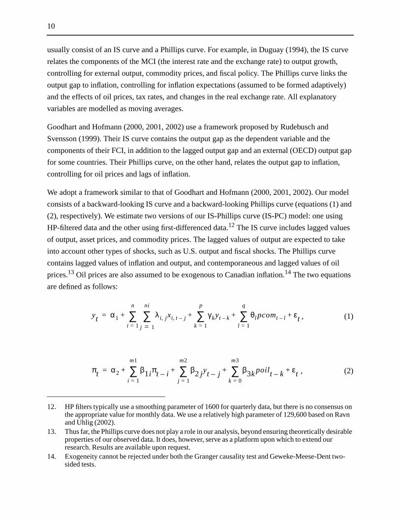
We adopt a framework similar to that of Goodhart and Hofmann (2000, 2001, 2002). Our m
consists of a backward-looking IS curve and a backward-looking Phillips curve (equations (1
(2), respectively). We estimate two versions of our IS-Phillips curve (IS-PC) model: one usi
HP-filtered data and the other using first-differenced data.12 The IS curve includes lagged values
of output, asset prices, and commodity prices. The lagged values of output are expected to
into account other types of shocks, such as U.S. output and fiscal shocks. The Phillips curv
contains lagged values of inflation and output, and contemporaneous and lagged values of
prices.13 Oil prices are also assumed to be exogenous to Canadian inflation.14 The two equations
are defined as follows:
, (1)
, (2)
12. HP filters typically use a smoothing parameter of 1600 for quarterly data, but there is no consenthe appropriate value for monthly data. We use a relatively high parameter of 129,600 based onand Uhlig (2002).
13. Thus far, the Phillips curve does not play a role in our analysis, beyond ensuring theoretically desproperties of our observed data. It does, however, serve as a platform upon which to extend ourresearch. Results are available upon request.
14. Exogeneity cannot be rejected under both the Granger causality test and Geweke-Meese-Dentsided tests.
yt α1 λi j, xi t j–,j 1=
ni
∑i 1=
n
∑ γkyt k–k 1=
p
∑ θl pcomt l–l 1=
q
∑ εt+ + + +=
πt α2 β1iπt i–i 1=
m1
∑ β2 j yt j–j 1=
m2
∑ β3kpoilt k–k 0=
m3
∑ εt+ + + +=

11
real
h of
, real
mium
.
se)
ther).
f an
tfalls,
1). In
arding
y
.
les in
e
ed by
ing
pact
del,
hich
wherey is the output gap in our HP-filtered specification (i.e., the percentage gap between
monthly GDP and its potential level, calculated as its HP-filtered trend) or the monthly growt
real GDP in our first-differenced specification.15 xi is componenti of the FCI, wherex = real
90-day commercial paper rate, real 10-year government bond rate, C-6 real exchange rate
residential housing prices, real S&P 500 stock price index, and AA corporate bond risk pre
or the U.S. high-yield bond spread.16 pcom is the real Bank of Canada commodity price index
In our Phillips curve,π is year-over-year core inflation (CPI excluding its eight most volatile
components and the effects of indirect taxes) andpoil is the monthly growth in crude oil prices.
3.2 FCIs based on generalized impulse-response functions
The IS-PC framework discussed in section 3.1 has a specification problem: the implicit (fal
assumption that the variables in the FCI are exogenous to output and inflation (and to each o
A natural way to solve this problem is to base our FCI weights on the impulse responses o
atheoretic VAR in which all the variables are treated as endogenous. This approach has pi
however, since the traditional procedure, suggested by Sims (1980), is to use a Cholesky
decomposition to orthogonalize the shocks (see, for example, Goodhart and Hofmann 200
doing so, the orthogonalized impulse-response functions are dependent on assumptions reg
the order in which each variable affects the others. In the case of an FCI that includes man
financial variables, all reacting instantaneously to shocks in the economy, there is no clear
guidance as to what set of assumptions should be made.
An appealing alternative is to base the weights on generalized impulse-response functions
Although orthogonalized impulse responses are not invariant to the reordering of the variab
the VAR, generalized impulse responses are. They are unique and take into full account th
historical patterns of correlations observed among different shocks. An FCI can be construct
weighting the variables according to their relative average impact on output over the follow
18 to 24 months, the period of time over which monetary policy is thought to have its full im
on output and inflation.
The generalized impulse-response function can be illustrated simply. Consider the VAR mo
15. A constant is included in equation (1) when using first-differenced data, but not when using HP-filtered data.
16. The U.S. high-yield spread is considered based on the results of Djoudad and Wright (2002), wsuggest a strong relationship between this spread and Canadian real GDP growth.

12
y
ls,
e
tcome
cks
at
tion
erties
o
the
n by
t,
(3)
where is an vector of jointly determined, dependent, stationar
variables and is an coefficient matrix. Under standard assumptions on the residua
equation (3) can be rewritten as the infinite moving-average representation,
, (4)
with and for .
An impulse-response function measures the effects of shocks at a given point in time on th
(expected) future values of variables in a dynamic system. It can best be described as the ou
of an experiment in which the time profile of the effect of a hypothetical vector of sho
of size hitting the economy at time is compared with a baseline profile
time , given the economy’s history.
We denote the known history of the economy up to time by the non-decreasing informa
set ; the generalized impulse-response function of at horizon is defined by
. (5)
Substituting equation (4) into (5), we have , which is independent of
but depends on the composition of shocks defined by .
Clearly, the appropriate choice of the hypothesized vector of shocks, , is central to the prop
of the impulse-response function. The traditional approach, suggested by Sims (1980), is t
resolve the problem surrounding the choice of by using a Cholesky decomposition of the
variance-covariance matrix of the residuals, ,
,
where is an lower triangular matrix. It is then easy to show that the vector of
orthogonalized impulse-response function of a unit shock to the th equation on is give
, where is an selection vector with unity as its th elemen
Xt Φi Xt i– εt , t+i 1=
p
∑ 1 2 … T,, , ,= =
Xt x1t x2t … xmt, , ,( )′= m 1×φi m m×
Xt Aiεt i– , ti 0=
∞
∑ 1 2 … T, , ,= =,
A0 I m= Ai 0= i 0<
m 1×δ δ1 δ2 … δm, , ,( )′= t
t n+
t 1–
Ωt 1– Xt n
GIX n δ Ωt 1–, ,( ) E Xt n+ εt = δ, Ωt 1–( ) E Xt n+ Ωt 1–( )–=
GIX n δ Ωt 1–, ,( ) Anδ=
Ωt 1– δ
δ
δΣ
PP' Σ=
P m m× m 1×j Xt n+
OIX n ej Ωt 1–, ,( ) AnPej= ej m 1× j

13
ry with
(1998).
oose
using
one
ctors)
nd
o-
ne
ctors
that
l
e
t
and zeros elsewhere. As stated earlier, these orthogonalized impulse-response functions va
the reordering of variables.
The alternative approach we follow in this paper was first suggested by Pesaran and Shin
They propose to use (4) directly, but instead of shocking all the elements of , we could ch
to shock only one element, say its th element, and integrate out the effects of other shocks
the historically observed distribution of errors. In this case, it is easily shown that the effect of
standard-error shock to the th equation at time on expected values of X at time is
(6)
where is the variance of and .
3.3 FCIs based on factor analysis
A third option in developing an FCI is to derive a linear weighted combination of financial
variables through factor analysis. Factor analysis extracts weighted linear combinations (fa
from a number of variables. This helps to detect the common structure in these variables a
remove “noise” created by irregular movements of certain variables at certain times. In a tw
variable example, the principal factor of the two variables is the least-squared regression li
between them. An advantage of this approach is that it does not depend on any model; a
disadvantage is that weights on individual variables are unknown.
Many studies have applied factor analysis to a large number of explanatory variables in
forecasting models. For example, Stock and Watson (1989, 1999) forecast GDP with a few fa
derived from 215 monthly indicators and find that the factor model outperforms various
benchmark models. Combining the information content in 334 Canadian and 110 U.S.
macroeconomic variables into a few representative factors, Gosselin and Tkacz (2001) find
factor models perform as well as more elaborate models in forecasting Canadian inflation.
English, Tsatsaronis, and Zoli (2003) construct an FCI by extracting factors (called financia
factors) from around 50 financial and real variables for the United States, Germany, and th
United Kingdom. They find that the financial factors provide considerable information abou
output and investment, but are not very informative about future inflation.
We apply factor analysis to a set of financial variables and derive our FCI from their primary
factor. We can express these variables as a function of the unknown factors:
, (7)
εt
j
j t t n+
GIX n δ Ω, t 1–,( ) σ jj AnΣej ,=
σ jj ej δ E εt ε jt = σ jj( )=
Xit λi L( )Ft eit+=

14
-linear
o
dict
d its
rs are
best of
whereXit is theith variable,Ft = (ft,..., ft-q) is an vector,q is the maximum number of lags,
, is the number of factors we would like to extract and is set to 10, andλi(L) is a
lag polynomial.17 The factorsft and disturbanceseit are assumed to be mean-zero stochastic
processes. The factorFt is estimated by the method of principal components. This involves
minimizing the sum of squared residuals of equation (7), which can be expressed as a non
objective function:
(8)
whereN is the number of variables andT is the sample length. After reorganizingF to the left-
hand side of equation (8), minimization is equivalent to maximizing , subject t
, where and eachλ is of dimension (see Stock and Watson
1999). The principal-components estimator ofF is thus
(9)
where is obtained by setting it equal to times the eigenvectors of the matrix
corresponding to its r largest eigenvalues.
4. Properties of Our FCIs
To evaluate our three FCIs, we consider five desirable properties or performance criteria18: the
consistency of each FCI’s estimated weight with economic theory, its graphical ability to pre
turning points in the business cycle, its dynamic correlation with the output gap (or monthly
growth in real GDP), its in-sample econometric fit with the output gap (or output growth), an
out-of-sample performance in forecasting the output gap (or output growth).
17. The marginal information content decreases rapidly after the first three to four factors. Ten factousually sufficient to capture the common variance of the entire data set.
18. Several combinations of variables were estimated within each of our three methodologies. Thethese are reported herein. The results of alternative formulations are available upon request.
r 1×r q 1+( )r= r
V F Λ,( )
Xit λi'Ft–( )2
t 1=
T
∑i 1=
N
∑NT
---------------------------------------------------,=
tr Λ' X'X( )Λ[ ]Λ'Λ( )N
-------------- I r= Λ λ0 … λq, ,( )= N 1×
FXΛ( )N
-------------,=
Λ N
12---
N N× X'X

15
st
ll lags
001,
t in the
ded
y
ion of
ll
er, to
s
FCIs
d rate,
ach of
d risk
d
n of
rcise
es are
4.1 FCIs based on a reduced-form model
In section 3.1, our IS-PC equations (1) and (2) are estimated separately using ordinary lea
squares (OLS) over the sample period 1981m1–2000m12.19 The lag structure for each variable
has been chosen by a general-to-specific strategy that begins with twelve lags and keeps a
between the first and the last significant lag.
We use two methods to derive the weights for the FCI. Following Goodhart and Hofmann (2
2002), we apply coefficients summarized across lags to each contemporaneous componen
FCI. In other words, the coefficients on each lag of a particular explanatory variable are ad
together and taken as the weight on that variable at timet. This method is subject to the criticism
that different asset prices have an impact on the real economy with varying lags, and that b
multiplying the summarized weights by the contemporaneous value of those variables, the
dynamics over time are ignored. In response to this criticism, we construct a separate vers
our FCI, allowing for the full dynamics of individual lags. This is similar to Batini and Turnbu
(2002), who use this method to construct a dynamic MCI for the United Kingdom.
In either case, we cannot make comparative statements regarding the size of the estimated
coefficients, because they are based on a reduced-form model and therefore partly reflect
contemporaneous relationships between explanatory variables. We find it desirable, howev
obtain weights and signs consistent with economic intuition, for communication purposes. A
such, Table 3 reports the estimated weights andp-values on our “summarized-weight” FCIs, using
alternatively HP-filtered data and first-differenced data.
As described for our general IS curve specification (equation (1)), each of our four IS-based
includes the real 90-day commercial paper rate, the real 10-year Government of Canada bon
the real C-6 exchange rate, real housing prices, and the real S&P 500 stock price index. E
these FCIs, however, differs somewhat in its use of variables to measure the corporate-bon
premium. Our HP-filterindividual-lag FCI contains the Canadian AA long-term corporate bon
spread, whereas our first-differenceindividual-lag FCI and both oursummarized-coefficient FCIs
use the U.S. high-yield spread.20
Regarding the first criterion by which we judge the performance of our FCI, further inspectio
Table 3 reveals that both our summarized-coefficient FCIs have estimated weights that are
19. Our estimation period ends in 2000 for the purpose of performing an out-of-sample forecast exeover 2001m1 to 2002m6, the results of which are reported later in this section.
20. Recall that both the Canadian AA corporate spread and the U.S. high-yield spread were tried asalternative measures of the risk premium in each FCI. The FCIs with the most desirable propertireported here.

16
CIs
of
CIs,
reted
rest
wth.
kness
Is. In
it
r our
-vis
d-
and
and
rsus
f the
th
001,
eaks
pliesmple.
consistent with economic theory. The traditional policy transmission channels upon which M
are built dictate that a higher short-term interest rate or higher exchange rate (appreciation
domestic currency) indicate a tighter policy stance. Indeed, in our summarized-coefficient F
both of these variables carry a negative coefficient. The long-term interest rate is often interp
as a proxy for future output growth: a higher long-term interest rate for a given short-term inte
rate, or a steeper yield curve, is well known to be a good indicator of higher future output gro
Accordingly, our FCIs have a positive summarized weight on the long-term interest rate.
Alternatively, a higher corporate bond risk premium, for a given long-term government bond
yield, suggests a rising cost of external financing for high-risk businesses and ensuing wea
in output via the credit channel. Thus, we expect a negative weight on this variable in our FC
fact, this is the case. Our FCIs suggest some combination of a wealth channel and/or cred
channel for monetary policy, in that both housing and stock prices hold positive estimated
coefficients. Furthermore, the test statistic put forth by Andrews (1993) suggests that our
estimated parameters, using either HP-filtered data or first-differenced data, are stable ove
sample.21 The estimation results for the specification of the FCI based on the IS curve with
individual lags and for the Phillips curve are also consistent with economic intuition and are
available upon request.
The second criterion by which we judge the performance of our FCI is visual inspection vis-à
the output gap (or output growth). Ideally, the FCI will perform as a leading indicator and
effectively signify business cycle turning points. Figure 1 compares our HP-filter summarize
coefficient FCI with the output gap. This FCI appears to follow the output gap fairly closely
often catches turning points in advance (e.g., upturns in 1986 and 1991, downturns in 1994
1999). Table 4 reports dynamic correlations, our third criterion, of all four IS-based FCIs ve
the output gap/output growth for various lag lengths. This table provides further evidence o
leading-indicator property of our HP-filter summarized-coefficient FCI, with a solid dynamic
correlation peaking at 0.606 two and three months in advance of the output gap.
Figure 2 compares our first-difference summarized-coefficient FCI (in annualized terms) wi
year-over-year real GDP growth. Visually, this FCI also generally performs well as a leading
indicator. Various turning points are clearly predicted in advance (e.g., upturns in 1995 and 2
downturns in 1983, 1987, 1994, and 1998). The correlation of this index with output growth p
at 0.609 four months in advance.
21. Specifically, a SupF statistic of 2.4 using HP-filtered data, and 2.2 using first-differenced data, imthat we cannot reject the null hypothesis of parameter stability at the 99 per cent level over our sa

17
ntly
g
ing
000).
our
gy—
real
nd
ith
ding-
f-
of the
a
.
cess,
a one-
I
,
n
ated
5,
h to
Figure 3 compares our HP-filter individual lag FCI with the output gap. This index is significa
more volatile than the other three IS-curve-based FCIs, primarily because of its dynamic la
structure. Nonetheless, it is able to follow the output gap fairly closely and does well in lead
some turning points (e.g., upturns in 1982, 1986, 1992, and 2001; downturns in 1989 and 2
This FCI has a slightly lower correlation with the output gap, peaking at 0.459 at a lead of f
months.
Figure 4 compares (in annualized terms) our final FCI based on the reduced-form methodolo
featuring first-differenced data and an individual, dynamic lag structure—with year-over-year
GDP growth. Similar to the preceding FCIs, this index follows output growth quite well over
some periods. This FCI also appears to lead various turning points (e.g., upturns in 1991 a
1996, downturns in 1987 and 1999–2000). However, the maximum correlation of this FCI w
output growth occurs with a lead of only one month, at a level of 0.583. In this respect, its lea
indicator property is not as strong as in our other three IS-curve-based FCIs.
The final two criteria by which we judge the performance of our FCIs are their in- and out-o
sample properties in a simple forecasting exercise. The exercise utilizes a rolling estimation
form
, (10)
wherey is the output gap (or year-over-year growth of real output),FCI is the particular FCI
under consideration, andk takes the value of 6, 9, 12, 18, 24. In other words, this forecast is
simple way of determining whether a given FCI helps explainy 6, 9, 12, 18, or 24 periods ahead
The length of the estimation sample for equation (10) is constant throughout the rolling pro
beginning in the early 1980s and ending at the last available observation, thereby providing
step-ahead forecast of the output gap (or output growth)k-steps ahead from our incorporated FC
data. Forecast observations are obtained for each month from January 2001 to June 2002
regardless of the value ofk in equation (6).22 This method of forecasting allows strict compariso
of results between FCIs for any particular value ofk, but not across values ofk (since the number
of observations used in the estimation varies). Recall that the weights for our FCIs are estim
22. For example, whenk = 24, estimation begins over 1983m1 to 2000m12, forecasting a value for2001m1. In the last iteration of the rolling regression, the estimation sample is 1984m6 to 2002mforecasting a value for 2002m6. Whenk = 6, the initial estimation period is 1981m6 to 2002m12 andthe final period is 1982m11 to 2002m5. Forecast values are still generated from 2001m1 throug2002m6.
yt α3 βFCIt k– εt+ +=
18
first
on a
on a
of the
isons
for
ent
ever,
output
up
h rate
is
, is
cient
point
nd
endent
from 1981 to 2000, to ensure the “out-of-sample” properties of our forecast over 2001 and the
half of 2002.
Table 5 reports the in-sample properties (coefficient on the FCI, itsp-value, and the adjusted R2)
as well as the mean squared forecast error (MSFE) for the forecasts using our FCIs based
reduced-form model. As one would expect, it is generally true that the size of the coefficient
given FCI, and the R2 value, fall ask increases. Conversely, thep-value of the coefficient on the
FCI and the mean squared forecast error both increase ask grows larger. The message behind
these numbers is that the further ahead one looks, the less of an explanation today’s value
FCI provides regarding the output gap (or output growth). As noted above, however, compar
across values ofk must be treated with caution, because of differing estimation sample sizes
eachk.
Our HP-filtered summarized-coefficient FCI shows up statistically significant at the 10 per c
level when explaining the output gap 6, 9, 12, and 18 months ahead. It is insignificant, how
when looking 24 months ahead. The largest coefficient on the FCI is 1.91 whenk = 6. In this case,
a one-point increase in the FCI translates into about a 1.91 percentage point increase in the
gap. This lag length also provides the maximum R2 of 0.311 for this FCI. Subsequent values ofk
give an R2 level that peters off in a fairly linear fashion to a value of approximately zero whenk =
24. Our first-difference summarized-coefficient FCI performs quite well in-sample, showing
statistically significant at all observed horizons (6, 9, 12, 18, and 24 months). Its maximum
coefficient is 1.20 at a horizon of six months, which suggests that the year-over-year growt
of real output half a year in the future will move 1.2 percentage points with each one-point
increase in today’s FCI value. The six-month horizon also gives the strongest R2 for this FCI at a
level of 0.310.
Our individual-lag FCI based on HP-filtered data shows up statistically significant ifk = 6, 9, 12,
and 18, but not whenk = 24. This FCI also has a stronger coefficient when it is significant. For
example, its largest coefficient, 2.83, comes atk = 6, which suggests that a one-point change in th
FCI translates into a 2.83 percentage point increase in the output gap half a year later. The
coefficient on this variable drops off quickly oncek reaches 18, and is insignificantly different
from zero whenk =24. Our other individual-lag-coefficient FCI, based on first-differenced data
statistically significant throughout our relevant horizon of 6 to 24 months. The strongest coeffi
on this FCI suggests that a one-point increase in the FCI translates into a 1.33 percentage
increase in the year-over-year growth of real output six months ahead.
Referring again to Table 5 for the reported MSFEs of our out-of-sample forecast exercise, a
keeping in mind that they can be compared only between FCIs that forecast the same dep

19
sing
r.
, 6
nths,
term
k
the
ts the
-
tent
icator
rt too
utput.
n the
d,
ator of
rm
ee
ssion.
iance of
warz
variable, our summarized-coefficient FCIs perform best (i.e., have the lowest MSFE) overall u
both HP-filter and first-difference definitions. The HP-filtered summarized-coefficient FCI
performs better at the 9-, 12-, and 18-month horizon in comparison with the HP-filtered
individual-lag FCI. At 6 and 24 months ahead, the individual-lag FCI performs slightly bette
Likewise, the first-difference summarized-coefficient FCI performs better at all relevant lags
through 24, compared with its individual-lag counterpart.
4.2 FCIs based on generalized impulse-response functions
Our VAR models are estimated with an 18-order lag structure.23 Our FCI weights have been
defined as the cumulative impact of a typical shock to each component on output over 24 mo
the period of time over which monetary policy is believed to have most of its impact. The
resulting FCI based on first-differenced data includes the short-term interest rate, the long-
interest rate, the exchange rate, the TSX index, housing prices, and the U.S. high-yield risk
spread. Its HP-filter counterpart is composed of the same six variables, except for the stoc
market, which is measured using the S&P 500. In Figure 5, the HP-filter FCI is plotted with
output gap. In Figure 6, the first-difference FCI is plotted with the output growth.
These FCIs can be viewed using the same five criteria described in section 4.1. Table 6 lis
weights for both impulse-response-function FCIs, and Figures 7 and 8 illustrate the impulse
response functions themselves. Both FCIs have positive weights on housing prices, consis
with expectations that high housing prices are a signal of excess demand and a leading ind
of strong construction activity. In the long run, however, output is adversely affected by an
increase in new housing prices (Figure 8). This suggests that high housing prices may dive
much capital from more-productive sectors of the economy, therefore depressing potential o
Both FCIs also place negative weights on the U.S. high-risk premium. A higher risk spread i
United States means tighter credit conditions and lower growth in that country going forwar
which, given the strong economic links between Canada and the United States, is an indic
lower growth in Canada as well. Our FCIs also both have a negative weight on the short-te
interest rate, which is consistent with the impact of monetary policy. The weights on the thr
remaining variables are of different signs in the different indexes; this deserves some discu
23. Akaike’s information criteria (AIC) and Schwarz’s criteria contradict each other. Schwarz’s critersuggest only one lag, whereas AIC suggests too many lags. This could be attributed to the presecointegration between the variables. Eighteen lags (six quarters) is in-between the AIC and Schsuggestions.

20
nd,
n the
ening
HP-
tput
ction
e HP-
he
. This
ave
ese
hese
he
y out-
g-term
ate
x and
riance
to
actor.
ed in
e HP-
1989
most
U.S.
, and
The negative weight on the stock market in the first-difference FCI is relatively quite small a
accordingly, should not be given much importance. This same FCI places a positive weight o
long-term interest rate, which suggests that a positive surprise in this interest rate, or a steep
yield curve, means stronger economic growth going forward. This weight is negative in the
filter index, but may be explained as a higher long-term interest rate increasing potential ou
still more than it increases short-run output. This is consistent with the impulse-response fun
shown in Figure 8. The negative weight on the exchange rate in the first-difference index is
consistent with the expected trade-balance effect of an appreciation. Its positive weight in th
filter FCI is plausible, because a higher exchange rate may decrease potential output, via t
higher cost of imported machinery and equipment, by more than it decreases actual demand
again is in line with the impulse-response function shown in Figure 8.
Table 4 shows that both the HP-filter and first-difference impulse-response function FCIs h
relatively dynamic correlations with output. This fact is also reflected in the in-sample fit of th
two FCIs (Table 7 and Figures 5 and 6). Overall, these FCIs perform fairly well according to t
criteria. In particular, the first-difference index leads the 1988, 1994, and 1999 downturns. T
HP-filter index is disappointing over the late 1990s. Both indexes also perform competitivel
of-sample at a relatively long forecast horizon (Table 7).
4.3 FCIs based on factor analysis
Our factor-analysis FCI based on HP-filtered data contains the short-term interest rate, lon
interest rate, exchange rate, housing prices, S&P/TSX composite index, and the AA corpor
spread. Its first-difference counterpart replaces the last two variables with the S&P 500 inde
the U.S. high-yield bond spread, respectively. Table 8 reports the percentage of common va
explained by each of the first four factors for these two indexes. The first factor captures 80
90 per cent of the common variance of output; thus, we specify our FCIs according to this f
Our two factor-analysis FCIs can be evaluated using four of the five performance criteria us
section 4.24 Figures 9 and 10 plot these two FCIs with their comparable GDP measures. Th
filter version (Figure 9) leads the recovery in 1982, 1986, 1993, 1995, and the downturn in
and 1994 by about one to three months, and coincides with the recession in 1982 and the
recent economic downturn. On the other hand, the first-difference version (Figure 10) with
equity and bond variables leads the boom in 1982, 1991, 1995, the busts in 1987 and 1999
24. Recall that, in a factor analysis, weights change over time and are unknown.

21
rning
tor
all
8-,
is are
ast,
cast
well-
-
ced
bles 3
ong-
), the
ear to
he
d, the
onth
-based
better
the pickup in 2002. On average, the first-difference FCI appears to pick up more economic tu
points and predict them with a longer lead than the HP-filter version.
Table 4 shows that the HP-filter version has a higher correlation with output than the first-
difference version at almost all horizons.
Table 7 shows the in-sample and out-of-sample performance of our two FCIs based on fac
analysis. The first-difference version is statistically significant in explaining future output at
horizons; the HP-filter version performs worse, with an insignificant coefficient at the 12-, 1
and 24-month horizons. The forecast-equation coefficients of all FCIs based on factor analys
relatively high compared with other methods of weighting. In terms of the out-of-sample forec
both versions perform better at a shorter horizon, with the HP-filter FCI yielding smaller fore
errors overall than the first-difference version.
4.4 Comparison of our FCIs
While each of our FCIs performs well in some respects, two specifications have particularly
rounded attributes according to our five performance criteria: the summarized-coefficient IS
curve-based FCI and the impulse-response-based FCI, both constructed using first-differen
data.
Both of these FCIs feature estimated weights and signs that are consistent with theory (Ta
and 6, respectively). While they each share several variables (the short-term interest rate, l
term interest rate, C-6 exchange rate, housing prices, and U.S. corporate bond risk premium
IS-curve-based FCI contains the S&P 500 index as a measure of stock prices, whereas the
impulse-response-based FCI utilizes the TSX composite index. Overall, the two indexes app
pick up roughly the same number of turning points in output growth.
The IS-curve-based FCI is more highly correlated with output at shorter horizons than the
impulse-response-based FCI. It also performs better in terms of in-sample significance in t
forecasting equation and in short-term forecasting 6 and 9 months ahead. On the other han
impulse-response-based FCI performs better in longer-term forecasts, at 12-, 18-, and 24-m
horizons.
Thus, both of these specifications are useful, depending on the task at hand. The IS-curve
FCI is better for predicting near-term output growth and the impulse-response-based FCI is
for predicting longer-term output growth.

22
me
hey
eflect
ave
ry
rest
only
effect
nd can
re
ables
e in the
lue in
ase
uch
ol in
we
e the
It is
vel.
5. Comparing the IS-Curve-Based FCI with the MCI
At first glance, an FCI resembles a traditional MCI in several ways. They share a similar na
and they contain similar variables. In fact, the FCI includes all of the variables of the MCI. T
are also similar in that their weights are usually derived using an IS-curve-based model to r
the relative impact of the variables on aggregate demand. Nevertheless, the two indexes h
significant differences.
The Bank of Canada’s MCI was created mainly to measure the effect of the Bank’s moneta
policy stance on the economy.25 The concept of an MCI is based on the belief that monetary
policy affects aggregate demand (and thus inflation via the output gap) mainly through inte
rate and exchange rate channels. On the other hand, the FCI contains asset prices that are
partially affected by monetary policy and yet may have an important impact on aggregate
demand. As discussed in section 1, this potential impact can take place through the wealth
or the credit channel. In a sense, the FCI is a much broader measure of the policy stance, a
be called the “financial stance.”
Another important difference between the two indexes is the way in which their variables a
detrended. In the HP-filter and first-difference versions of our FCI, we assume that the vari
are non-stationary. The MCI, in contrast, implicitly assumes that the interest rate and the
exchange rate are stationary. The MCI is expressed as the weighted average of the chang
interest rate from its value in January 1987 and the change in the exchange rate from its va
the same time period. It is hard to believe that the economy was in equilibrium during the b
period and that the nature of equilibrium has not changed since.26
In addition, the signs of the MCI and the FCI are interpreted differently. The MCI is defined s
that a higher value means a tighter monetary policy, whereas a higher FCI signifies a more
accommodative financial stance.
Despite its desirable features, the FCI must outperform the MCI empirically to be a useful to
the conduct of monetary policy. To investigate the properties and performance of the MCI,
perform a set of exercises similar to those we performed for our FCIs. Specifically, we explor
MCI’s graphical representations, correlations, and forecasting ability with respect to output.
25. While the Bank of Canada (Freedman 1995) refers to “using the MCI as an operational target ofmonetary policy,” the importance of the MCI in setting monetary policy has been largely de-emphasized.
26. In practice, however, more emphasis is usually placed on the change in the MCI instead of its leThe problem of non-stationarity is, in a sense, addressed in this way. See also section 6.

23
el,
e 11
wth.
ms to
the
at
is
GDP
put
lly
nd 24
ns,
the
owth
ased
MCI
, their
se the
m
th.
tain:
important to note, however, that we focus on the MCI’s first-difference as opposed to its lev
given that changes in policy stance are more clearly reflected in the former measure. Figur
plots the first-differenced MCI and our IS-curve-based FCI against year-over-year GDP gro
Graphically, our FCI seems to do much better at tracing the dynamics of GDP growth and
capturing the turning points in the business cycle. The first-differenced MCI, in contrast, see
capture excessive quarter-over-quarter noise.
Table 9 shows the dynamic correlation between the MCI and GDP growth. The MCI yields
wrong sign in the correlation with output growth, except for the correlation with output growth
12 and 18 months. Even at those two horizons, the dynamic correlation with output growth
much lower than that between our FCIs and output growth.
Table 10 shows the results of the MCI-based forecast of the output gap and year-over-year
growth. The MCI yields the wrong sign in forecasting the output gap at all horizons and out
growth 6 and 9 months ahead. Compared with our FCIs, the MCI is generally less statistica
significant, and produces a lower adjusted R2. In terms of forecasting the output gap, our first-
difference IS-curve-based FCI outperforms the MCI 6, 9, and 12 months ahead, but not 18 a
months ahead. Nevertheless, our FCI that uses weights from the impulse-response functio
which has been found to forecast better in longer horizons, produces a smaller MSFE than
MCI 24 months ahead. Similarly, our IS-curve-based FCI does better in forecasting output gr
than the MCI in shorter horizons (6 to 18 months ahead), whereas the impulse-response-b
FCI does better in the longer horizon (24 months ahead). Overall, our FCIs outperform the
under our set of criteria.
6. Interpreting the FCI as a Measure of Financial Stance
Given that our best FCIs are a weighted sum of the first-differences of our chosen variables
interpretation as a measure of stance is not clear a priori. In this section we argue that, becau
first difference of a I(1) series is simply its deviation from its stochastic trend or its equilibriu
value, the higher the FCI, the looser the “financial stance” and the higher the expected grow
Decomposing each variable in our FCI into its permanent and transitory component, we ob
,
where the permanent component is the equilibrium value of the variable, , and is its
transitory component or its deviation from equilibrium. Take the first difference of :
.
xt xte
tct+=
xte
tct
xt
∆xt xte
xt 1–e
–( ) tct tct 1––+=

24
nthly
of the
rium
e
s a
s the
ices
he
are
ed on
f the
using
nt
istent
ints,
and
wth).
the
take
000,
- and
e HP-
l
Then assume that the equilibrium changes very slowly, so that we can approximate the mo
change, , as:
.
This assumption cannot be made if is large. It is more complicated to compare the value
FCI two years ago with its value today in terms of monetary policy stance, since the equilib
values have probably changed over that period.27 But from one monetary policy fixed
announcement date to another, it seems reasonable to assume that equilibrium levels of th
variables have not changed much, if at all.
Under this assumption, a positive change in the short-term interest rate, for example, mean
tighter money market. Since the short-term interest rate is negatively weighted, it decrease
FCI, which implies lower expected output growth. Symmetrically, an increase in housing pr
directly stimulates housing supply, and, indirectly, through the credit channel, it increases t
borrowing capacity of consumers, which stimulates consumption. Because housing prices
positively weighted in the FCI, a higher level is indicative of a looser “financial stance” and
signals higher output growth.
7. Conclusion
We have provided a survey of the existing FCIs and proposed several FCIs for Canada bas
three different approaches. Each approach is intended to address one or more criticisms o
MCI and existing FCIs. For each approach, we experimented with one set of data detrended
an HP filter and a second set detrended by first-differencing. We then evaluated the differe
versions of our FCIs based on five criteria: estimated weights on components that are cons
with theory, graphical leading-indicator properties with respect to business cycle turning po
strong dynamic correlation versus the output gap (or monthly growth in real GDP), and in-
out-of-sample performance in a simple forecasting exercise of the output gap (or output gro
Our first approach derived its weights from an IS-Phillips curve framework in two ways: using
sum of the coefficients on the lags of the variables, and including individual lags in the FCI to
into account the dynamics of those variables over time. Using monthly data from 1981 to 2
we found that housing prices, equity prices, and bond risk premiums, in addition to the short
long-term interest rates and the exchange rate, are significant in explaining output. In both th
filter and first-difference specifications, estimated parameters are consistent with theoretica
27. The same critique applies to the MCI.
∆xt
∆xt tct tct 1––( )=
∆t

25
use
adian
well-
the
erm
m
t over
a we
asting
hts of
.
expectations. Consistent with Djoudad and Wright (2002), we also found that the FCIs that
U.S. stock prices and high-yield bond spreads perform better than the ones that include Can
stock prices and investment bond spreads.
Our second and third approaches derived weights based on generalized impulse-response
functions from a VAR and a factor analysis, respectively.
Out of our eight FCIs based on all three approaches, two specifications showed particularly
rounded attributes considering several different criteria. The FCI that derived its weights from
summed coefficients of an IS curve using first-differenced data served the best as a short-t
(less than one year) predictor of output growth, whereas the FCI that derived its weights fro
VAR impulse-response functions using first-differenced data served the best to predict outpu
the longer term (one to two years). Our FCIs also outperformed the MCI in most of the criteri
considered.
Future research can further investigate the properties of these FCIs by comparing their forec
performance with benchmark univariate models. It may also be possible to derive the weig
the FCIs from a large-scale macro model in which financial variables play an important role

26
n
netary
s
omic
Can-
htNo.
nism
ndi-
s ofumn
ondi-pers
ading
the
Bibliography
Andrews, D.W.K. 1993. “Test for Parameter Instability and Structural Change with UnknowChange Point.”Econometrica 61(4): 821–56.
Ball, L. 1999. “Policy Rules for Open Economies.” InMonetary Policy Rules, edited by J.B. Taylor.University of Chicago Press for NBER.
Batini, N. and K. Turnbull. 2002. “A Dynamic Monetary Conditions Index for the UK.”Journalof Policy Modelling 24: 257–81.
Bernanke, B.S. and A.S. Blinder. 1992. “The Federal Funds Rates and the Channels of MoTransmission.”American Economic Review 82: 901–21.
Bernanke, B. and M. Gertler. 1989. “Agency Costs, Collateral and Business Fluctuations.”Ameri-can Economic Review 79: 14–31.
———. 1999. “Monetary Policy and Asset Price Volatility.” Federal Reserve Bank of KansaCity Economic Review, Fourth Quarter 1999: 17–51.
Carmichael, T. 2002. “Canada’s Financial Conditions Point to Recovery.” J.P. Morgan. EconResearch Note: February 7.
Cozier, B. and G. Tkacz. 1994. “The Term Structure and Real Activity in Canada.” Bank of ada Working Paper No. 1994-03.
Dudley, W. and J. Hatzius. 2000. “The Goldman Sachs Financial Conditions Index: The RigTool for a New Monetary Policy Regime.” Goldman Sachs Global Economics Paper 44.
Duguay, P. 1994. “Empirical Evidence on the Strength of the Monetary Transmission Mechain Canada.”Journal of Monetary Economics 33: 39–61.
Eika, K.H., N.R. Ericsson, and R. Naymoen. 1996. “Hazards in Implementing a Monetary Cotions Index.”Oxford Bulletin of Economics and Statistics 58(4): 765–90.
English, W., K. Tsatsaronis, and E. Zoli. 2003. “Assessing the Predictive Power of MeasureFinancial Conditions for Macroeconomic Variables.” Paper presented at the BIS AutEconomists’ Meeting, 9-10 October, BIS papers, forthcoming.
Ericsson, N., E. Jansen, N. Kerbeshian, and R. Nymoen. 1998. “Interpreting a Monetary Ctions Index in Economic Policy.” In Bank for International Settlements Conference PaVol 6.
Estrella, A. and F.S. Mishkin. 1998. “Predicting U.S. Recessions: Financial Variables as LeIndicators.”Review of Economics and Statistics 80: 45–61.
Fama, E.F. 1981. “Stock Returns, Real Activity, Inflation and Money.”American EconomicReview 71: 545–65.
Freedman, C. 1995. “The Role of Monetary Conditions and the Monetary Conditions Index inConduct of Policy.”Bank of Canada Review (Autumn): 53–60.

27
l.”
Set-
Infla-
licy.”
y.”Policy,
oyal
i-
iga-
em-
riate
ada
Gauthier, C. and F. Li. 2004. “Linking Financial Markets and the Real Economy: BEAM ModeBank of Canada. Unpublished manuscript.
Gerlach, S. and F. Smets. 2000. “MCIs and Monetary Policy.”European Economic Review 44:1677–1700.
Gertler, M., M. Goodfriend, O. Issing, and L. Spaventa. 1998.Asset Prices and Monetary Policy:Four Views. Centre for Economic Policy Research (CEPR) and Bank for Internationaltlements. CEPR: London.
Goodhart, C. 2001. “What Weight Should be Given to Asset Prices in the Measurement of tion?” The Economic Journal 111(June): 335–56.
Goodhart, C. and B. Hofmann. 2000. “Financial Variables and the Conduct of Monetary PoSveriges Riksbank Working Paper No. 112.
———. 2001. “Asset Prices, Financial Conditions, and the Transmission of Monetary PolicPaper prepared for the conference on Asset Prices, Exchange Rates, and MonetaryStanford University, 2-3 March.
———. 2002. “Asset Prices and the Conduct of Monetary Policy.” Paper presented at the REconomic Society Annual Conference, University of Warwick, 25-27 March.
Gosselin, M. and G. Tkacz. 2001. “Evaluating Factor Models: An Application to ForecastingInflation in Canada.” Bank of Canada Working Paper No. 2001-18.
Guay, A. and P. St-Amant. 1996.Do Mechanical Filters Provide a Good Approximation of Busness Cycles? Technical Report No. 78. Ottawa: Bank of Canada.
Harvey, C.R. 1989. “Forecasts of Economic Growth from the Bond and Stock Markets.”Finan-cial Analyst Journal 45(5): 38–45.
Hodrick, R.J. and E.C. Prescott. 1980. “Postwar U.S. Business Cycles: an Empirical Investtion.” Discussion Paper No. 451, Carnegie Mellon University.
Lack, C. 2002. “A Financial Conditions Index for Switzerland.” Paper prepared for the BISAutumn Central Bank Economist Meeting of 14-15 October 2002.
Macroeconomic Advisers. 1998. “From the U.S. Economic Outlook.” Technical Notes: Septber 5.
Mayes, D. and M. Virén. 2001. “Financial Conditions Indexes.” Bank of Finland DiscussionPaper No. 2001-17.
Modigliani, F. 1971. “Monetary Policy and Consumption.” InConsumer Spending and MonetaryPolicy: The Linkages. Federal Reserve Bank of Boston.
Pesaran, M.H. and Y. Shin. 1998. “Generalized Impulse Response Analysis in Linear MultivaModels.”Economics Letters 58: 17–29.
Pichette, L. and D. Tremblay. 2003. “Are Wealth Effects Important for Canada?” Bank of CanWorking Paper No. 2003-30.

28
d.”
dica-R.
d atarket
ing
Ravn, M.O. and H. Uhlig 2002. “Notes on Adjusting the Hodrick-Prescott Filter for the Fre-quency of Observations.”The Review of Economics and Statistics 84(2): 371–80.
Rudebusch, G. and L. Svensson. 1999. “Policy Rules for Inflation Targeting.” InMonetary PolicyRules, edited by J.B. Taylor. University of Chicago Press for NBER.
Sims, C.A. 1980. “A Comparison of Interwar and Postwar Cycles: Monetarism ReconsidereAmerican Economic Review 70 (May): 250–57.
Stock, J.H. and M.W. Watson. 1989. “New Indexes of Coincident and Leading Economic Intors.” In Macroeconomic Annual,edited by O.J. Blanchard and S. Fischer, 352–94. NBE
———. 1999. “Forecasting Inflation.”Journal of Monetary Economics 44: 293–335.
———. 2000. “Forecasting Output and Inflation: The Role of Asset Prices.” Paper presentethe Sverriges Riksbank and Stockholm School of Economics Conference on Asset Mand Monetary Policy, Stockholm, June.
Zhang, Z. 2002. “Corporate Bond Spreads and the Business Cycle.” Bank of Canada WorkPaper No. 2002-15.

29
Table 1: Composition of Canadian Household Total Assets
YearsProperty(per cent)
Equitya
(per cent)
a. Including mutual funds.Source: Statistics Canada Cansim matrix 751
Bonds(per cent)
Life insuranceand pension(per cent)
Others(per cent)
1981–1985 36 10 5 14 35
1986–1990 36 10 5 17 32
1991–1995 36 11 4 19 30
1996–2000 34 14 3 22 27

30
c Studies
DetrendingSource ofweights
ange from a base period IS curve
r” to the BoC index IMF’s and OECD’smacro models
f real interest andge rate; first-difference
rest
IS curve (singleequation)
wn Simple average
t and exchange ratesion from historic mean)
Fed macro model
ion from mean dividedance
Simple averagec
CI.
ecified; referred to asical adjustment”
Washington Uni-versity MacroModel (WUMM)
ion from trend: long-an for interest rate; lin-nd for exchange rateuse prices; HP filter for
ricesd
P filter.
1) Reduced-form ISand PC model2) Impulse-response functionsof a VAR
ifference Shocks to a:1) Restricted2) Structuralmacro model
Table 2: MCI and FCIs Constructed by Orgarizations and Academi
Organizations/studiesShort-term
ratesLong-term rates
Exchangerates
Equity marketOther
variables
Bank of Canada Nominal 90 CP Nominal C-6 Ch
Banque de France forG-7
Real 3-monthmarket rate
Real 10-year govern-ment rate
Real effec-tive
“simila
Mayes and Virén,(2001) for 17 countries
Real 3-monthmarket rate
Real bilat-eral vs. U.S.
Real stock price Real houseprices
Level oexchanfor the
Goldman Sachs forCanada
Real 3-monthmarket rate
Real effec-tive
Measure of stockvaluation
Yield curve Unkno
Goldman Sachs (2000)
for U.S.a
a. See Dudley and Hatzius (2000).
Real 3-monthLIBOR
Real A-rated corpo-rate, indexed
Real trade-weighted
Equity mkt cap/GDP ratio
Interes(deviat
J.P. Morgan for Canada
(2002)b
b. See Carmichael (2002).
Nominal 3-month marketrate
10-year corporatespread
Nominal C-6 Nominal TSXindex
(1) Yield curve(2) M1(3) M2++
Deviatby vari
c. The short-term interest rate and exchange rate are combined as one component to mimic the Bank of Canada’s M
MacroeconomicAdvisers (1998) for theU.S.
Real fed fundsrate
Real 10-year Treas-ury yield
Real (1) Dividend/ priceratio(2) Householdequity wealth
Not sp“techn
Goodhart and Hof-mann (2001) for G-7
Real 3-monthmarket rate
Real effec-tive
Real stock price Real propertyprices
Deviatrun meear treand ho
stock p
d. Goodhart and Hofmann (2002) construct an FCI only for the U.K., in which all variables are detrended using the H
Lack (2002) Real 3-monthLIBOR
Real trade-weighted
Real propertyprices
First-d

31
. Neither
Table 3: Specification of FCIs Based on IS Curve with Summarized Lagsa
a. Both regressions contain contemporaneous and lagged values of commodity prices, as well as lags of the output gapof these variables is included in the calculation of the FCIs.
VariableFCI—HP filter FCI—First-difference
Weight Weight
Constant - 0.137
Real 90-day commercial paper ratet -0.118 -0.164
Real 10-year Government of Canadabond ratet
0.288 0.554
Real C-6 exchange ratet -0.044 -0.111
Real housing price indext 0.073 0.108
Real S&P 500 stock indext 0.019 0.067
U.S. high-yield risk spreadt -0.224 -0.194
Adjusted R2 94.0 21.8
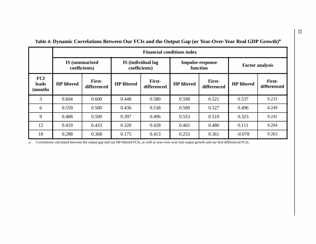
32
er-Year Real GDP Growth)a
th and our st-differenced FCIs.
Factor analysis
edHP filtered First-
differenced
21 0.537 0.233
27 0.496 0.249
10 0.323 0.241
80 0.111 0.204
61 -0.078 0.263
Table 4: Dynamic Correlations Between Our FCIs and the Output Gap (or Year-Ov
a. Correlations calculated between the output gap and our HP-filtered FCIs, as well as year-over-year real output growfir
Financial conditions index
IS (summarizedcoefficients)
IS (individual lagcoefficients)
Impulse-responsefunction
FCIleads
(monthsHP filtered
First-differenced
HP filteredFirst-
differencedHP filtered
First-differenc
3 0.604 0.600 0.448 0.580 0.598 0.5
6 0.559 0.580 0.436 0.538 0.589 0.5
9 0.488 0.500 0.397 0.496 0.553 0.5
12 0.419 0.433 0.320 0.428 0.465 0.4
18 0.288 0.368 0.175 0.413 0.253 0.3

33
s fore-
Table 5: Properties of FCI-Based Forecasting Exercise (IS-Based FCIs)
FCI based onStepsahead
Coefficient onFCIa,b
a. Values in parentheses denotet-test statistical significance.b. Estimated over entire sample: 1981 to 2000.
Adjusted R2 b MSFEb,c
c. RMSE calculated using a rolling forecast with an initial sample beginning in 1981. Output gap (or real GDP growth) icast over 2001m1 to 2002m6.
IS curveHP-filtered data
Summed coefficients
6 1.91 (0.00) 0.311 0.814
9 1.62 (0.00) 0.223 0.315
12 1.40 (0.00) 0.170 0.578
18 0.97 (0.06) 0.099 1.363
24 0.23 (0.64) 0.002 1.098
IS curveFirst-differenced dataSummed coefficients
6 1.20 (0.00) 0.310 0.783
9 0.97 (0.00) 0.206 1.111
12 0.84 (0.00) 0.156 1.514
18 0.73 (0.01) 0.121 2.180
24 0.60 (0.02) 0.083 2.505
IS curveHP-filtered data
Indiv. lag coefficients
6 2.83 (0.00) 0.183 0.578
9 2.63 (0.00) 0.160 0.847
12 2.10 (0.00) 0.105 1.145
18 1.24 (0.05) 0.043 1.401
24 0.48 (0.50) 0.003 1.097
IS curveFirst-differenced dataIndiv. lag coefficients
6 1.33 (0.00) 0.256 1.233
9 1.20 (0.00) 0.213 1.274
12 1.05 (0.01) 0.162 1.526
18 1.04 (0.01) 0.167 2.207
24 0.92 (0.04) 0.134 2.624

34
Table 6: FCI Weights as Derived From VAR Generalized Impulse-Response Function
VariableFCI—HP filter FCI—First-difference
Coefficient Coefficient
Real 90-day commercial paperratet
-2.089 -0.15
Real 10-year Government ofCanada bond ratet
-1.75 0.249
Real C-6 exchange ratet 0.066 -0.21
Real housing price indext 7.95 0.38
Real S&P 500 stock index 0.54
Real TSX composite indext -0.02
U.S. high-yield risk spreadt -9.22 -0.74
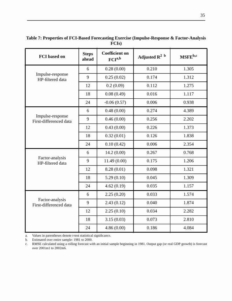
35
is
forecast
Table 7: Properties of FCI-Based Forecasting Exercise (Impulse-Response & Factor-AnalysFCIs)
FCI based onStepsahead
Coefficient onFCIa,b
a. Values in parentheses denotet-test statistical significance.b. Estimated over entire sample: 1981 to 2000.
Adjusted R2 b MSFEb,c
c. RMSE calculated using a rolling forecast with an initial sample beginning in 1981. Output gap (or real GDP growth) isover 2001m1 to 2002m6.
Impulse-responseHP-filtered data
6 0.28 (0.00) 0.210 1.305
9 0.25 (0.02) 0.174 1.312
12 0.2 (0.09) 0.112 1.275
18 0.08 (0.49) 0.016 1.117
24 -0.06 (0.57) 0.006 0.938
Impulse-responseFirst-differenced data
6 0.48 (0.00) 0.274 4.389
9 0.46 (0.00) 0.256 2.202
12 0.43 (0.00) 0.226 1.373
18 0.32 (0.01) 0.126 1.838
24 0.10 (0.42) 0.006 2.354
Factor-analysisHP-filtered data
6 14.2 (0.00) 0.267 0.768
9 11.49 (0.00) 0.175 1.206
12 8.28 (0.01) 0.098 1.321
18 5.29 (0.10) 0.045 1.309
24 4.62 (0.19) 0.035 1.157
Factor-analysisFirst-differenced data
6 2.25 (0.20) 0.033 1.574
9 2.43 (0.12) 0.040 1.874
12 2.25 (0.10) 0.034 2.282
18 3.15 (0.03) 0.073 2.810
24 4.86 (0.00) 0.186 4.084
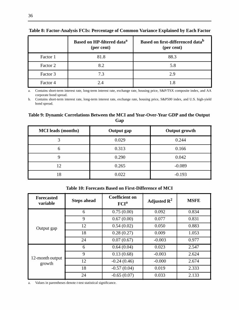
36
and AA
igh-yield
Table 8: Factor-Analysis FCIs: Percentage of Common Variance Explained by Each Factor
Based on HP-filtered dataa
(per cent)
a. Contains short-term interest rate, long-term interest rate, exchange rate, housing price, S&P/TSX composite index,corporate bond spread.
Based on first-differenced datab
(per cent)
b. Contains short-term interest rate, long-term interest rate, exchange rate, housing price, S&P500 index, and U.S. hbond spread.
Factor 1 81.8 88.3
Factor 2 8.2 5.8
Factor 3 7.3 2.9
Factor 4 2.4 1.8
Table 9: Dynamic Correlations Between the MCI and Year-Over-Year GDP and the OutputGap
MCI leads (months) Output gap Output growth
3 0.029 0.244
6 0.313 0.166
9 0.290 0.042
12 0.265 -0.089
18 0.022 -0.193
Table 10: Forecasts Based on First-Difference of MCI
Forecastedvariable
Steps aheadCoefficient on
FCIa
a. Values in parentheses denotet-test statistical significance.
Adjusted R2 MSFE
Output gap
6 0.75 (0.00) 0.092 0.834
9 0.67 (0.00) 0.077 0.831
12 0.54 (0.02) 0.050 0.883
18 0.28 (0.27) 0.009 1.053
24 0.07 (0.67) -0.003 0.977
12-month outputgrowth
6 0.64 (0.04) 0.023 2.547
9 0.13 (0.68) -0.003 2.624
12 -0.24 (0.46) -0.000 2.674
18 -0.57 (0.04) 0.019 2.333
24 -0.65 (0.07) 0.033 2.133

37
Output GapFCI
Figure 1IS-Based HP-Filter FCI and the Output Gap - Summarized Coefficients
Year-Over-Year Real GDP GrowthFCI (annualized)
Figure 2IS-Based First-Difference FCI and Real Output Growth - Summarized Coefficients

38
Output GapFCI
Figure 3IS-Based HP-Filter FCI and the Output Gap - Individual Lag Coefficients
Year-Over-Year Real GDP GrowthFCI (annualized)
Figure 4IS-Based First-Difference FCI and Real Output Growth - Individual Lag Coefficients

39
Output GapFCI
Figure 5Impulse-Response-Based HP-Filter FCI and the Output Gap
Year-Over-Year Real GDP GrowthFCI (annualized)
Figure 6Impulse-Response-Based First-Difference FCI and Real Output Growth

40
Figure 7Impulse Response of Output - Real HP-Filtered Data
(solid line - year-over-year real GDP growth ; dashed line - forecast)
90-day Commercial Paper Rate 10-year GOC bond
C6 Exchange Rate S&P 500 Stock Index
New Housing Price Index U.S. High-Yield Risk Premium
Figure 8Impulse Response of Output - Real First-Differenced Data
(solid line - year-over-year real GDP growth ; dashed line - forecast)
90-day Commercial Paper Rate 10-year GOC bond
C6 Exchange Rate S&P/TSX Composite Stock Index
New Housing Price Index U.S. High-Yield Risk Premium

41
Output GapFCI
Figure 9Factor-Analysis-Based HP-Filter FCI and the Output Gap
Year-Over-Year Real GDP GrowthFCI (annualized)
Figure 10Factor-Analysis-Based First-Difference FCI and Real Output Growth

42
Year-Over-Year Real GDP GrowthFirst-Difference of MCIFirst-Difference IS-Based FCI
Figure 11MCI, FCI and Output Growth

Bank of Canada Working PapersDocuments de travail de la Banque du Canada
Working papers are generally published in the language of the author, with an abstract in both officiallanguages.Les documents de travail sont publiés généralement dans la langue utilisée par les auteurs; ils sontcependant précédés d’un résumé bilingue.
Copies and a complete list of working papers are available from:Pour obtenir des exemplaires et une liste complète des documents de travail, prière de s’adresser à:
Publications Distribution, Bank of Canada Diffusion des publications, Banque du Canada234 Wellington Street, Ottawa, Ontario K1A 0G9 234, rue Wellington, Ottawa (Ontario) K1A 0G9E-mail: [email protected] Adresse électronique : [email protected] site: http://www.bankofcanada.ca Site Web : http://www.banqueducanada.ca
20042004-21 Exchange Rate Pass-Through and the Inflation
Environment in Industrialized Countries: AnEmpirical Investigation J. Bailliu and E. Fujii
2004-20 Commodity-Linked Bonds: A Potential Means forLess-Developed Countries to Raise Foreign Capital J. Atta-Mensah
2004-19 Translog ou Cobb-Douglas? Le rôle des duréesd’utilisation des facteurs E. Heyer, F. Pelgrin and A. Sylvain
2004-18 When Bad Things Happen to Good Banks:Contagious Bank Runs and Currency Crises R. Solomon
2004-17 International Cross-Listing and the Bonding Hypothesis M. King and D. Segal
2004-16 The Effect of Economic News on Bond Market Liquidity C. D’Souza and C. Gaa
2004-15 The Bank of Canada’s Business OutlookSurvey: An Assessment M. Martin and C. Papile
2004-14 National Saving–Investment Dynamics andInternational Capital Mobility F. Pelgrin and S. Schich
2004-13 Contraintes de liquidité et capital humaindans une petite économie ouverte F. Pelgrin
2004-12 Durées d’utilisation des facteurs et fonction deproduction : une estimation par la méthode desmoments généralisés en système E. Heyer, F. Pelgrin, and A. Sylvain
2004-11 Estimating New Keynesian Phillips CurvesUsing Exact Methods L. Khalaf and M. Kichian
2004-10 Public Venture Capital and Entrepreneurship O. Secrieru and M. Vigneault
2004-9 Estimating Policy-Neutral Interest Rates for CanadaUsing a Dynamic Stochastic General-EquilibriumFramework J.-P. Lam and G. Tkacz
2004-8 The Economic Theory of Retail Pricing: A Survey O. Secrieru
2004-7 The Demand for Money in a Stochastic Environment J. Atta-Mensah
Top Related