File: MANUAL.TXT

PPPPP EEEEEE N N EEEEEE L OOOO PPPPP EEEEEEP P E NN N E L O O P P EP P E N N N E L O O P P EPPPPP EEEE N N N EEEE L O O PPPPP EEEEP E N NN E L O O P EP EEEEEE N N EEEEEE LLLLLL OOOO P EEEEEE

(version 2003).

F. Salvat, J.M. Fernandez-Varea and J. Sempau

Facultat de Fisica (ECM). Universitat de Barcelona.Diagonal 647. 08028 Barcelona. Spain

---- GENERAL INFORMATION ----

The FORTRAN 77 code system PENELOPE performs Monte Carlo simulationof coupled electron-photon transport in arbitrary materials. Initially,it was devised to simulate the PENetration and Energy LOss of Positronsand Electrons in matter; photons were introduced later. The adoptedscattering model allows the simulation of electron/positron and photontransport in the energy range from 100 eV to 1 GeV. PENELOPE generatesrandom electron-photon showers in complex material structures consistingof any number of distinct homogeneous regions (bodies) of differentcompositions.

PENELOPE allows the user to write her/his own simulation program,with arbitrary geometry and scoring, without previous knowledge of theintricate features of scattering and transport theories. PENELOPE hasbeen devised to do a great part of the simulation work. The MAINprogram, which is provided by the user, only has to control theevolution of the simulated tracks and keep score of the relevantquantities.

For the sake of brevity, we use the term ’particle’ to refer toeither electrons, positrons or photons. Interactions with the mediumcause particles to lose energy, change their direction of movement and,occasionally, produce secondary particles. PENELOPE incorporates ascattering model that combines information from numerical databases withsimple analytical differential cross section models. The consideredinteractions and the corresponding differential cross sections are thefollowing:A) Elastic scattering of electrons and positrons: MW differential

cross section model with parameters determined from the mean freepath and first and second transport mean free paths read from the

input material definition file.B) Inelastic collisions of electrons and positrons: Born differential

cross section obtained from the Sternheimer-Liljequist generalizedoscillator strength model, including the density effect correction.The differential cross section is renormalized to reproduce thecollision stopping power read from the input file.

C) Bremsstrahlung emission by electrons and positrons: the energy ofthe emitted photons is sampled from numerical energy-loss spectraobtained from the scaled cross-section tables of Seltzer and Berger,renormalized to reproduce the radiative stopping power read from theinput file.The intrinsic angular distribution of emitted photons is describedby an analytical expression with parameters determined by fittingthe benchmark partial-wave shape functions of Kissel, Quarles andPratt.

D) Positron annihilation: Heitler differential cross section fortwo-photon annihilation in flight.

E) Inner-shell ionization by electron and positron impact: total crosssections obtained from an optical-data (virtual quanta) model.Correlations between the energy lost by the projectile and theemitted fluorescent radiation (Auger electrons and x-rays) aredisregarded.

F) Coherent (Rayleigh) scattering of photons: Born differential crosssection with an analytical atomic form factor.

G) Incoherent (Compton) scattering of photons: differential crosssection calculated using the relativistic impulse approximation withanalytical one-electron Compton profiles.

H) Photoelectric absorption of photons: total atomic cross sections andK- and L-shell partial cross sections from the LLNL Evaluated PhotonData Library. The initial direction of photoelectrons is sampledfrom Sauter’s K-shell hydrogenic differential cross section.

I) Electron-positron pair production: total cross sections obtainedfrom the XCOM program of Berger and Hubbell. The initial kineticenergies of the produced particles are sampled from the Bethe-Heitler differential cross section, with exponential screening andCoulomb correction, empirically modified to improve its reliabilityfor energies near the pair-production threshold.

The simulation of photon transport follows the usual detailedprocedure, i.e. all the interaction events in a photon history aresimulated in chronological succession.

The simulation of electron and positron tracks is performed by meansof a mixed (class II) algorithm. Individual hard elastic collisions,hard inelastic interactions and hard bremsstrahlung emission aresimulated in a detailed way, i.e. by random sampling from thecorresponding restricted differential cross sections. The track of aparticle between successive hard interactions, or between a hardinteraction and the crossing of an interface (i.e. a surface thatseparates two media with different compositions) is generated as aseries of steps of limited length (see below). The combined effect ofall (usually many) soft interactions that occur along a step is

2

simulated as a single ’artificial’ soft event (a random hinge) where theparticle loses energy and changes its direction of motion. The energyloss and angular deflection at the hinge are generated according to amultiple scattering approach that yields energy loss distributions andangular distributions with the correct mean and variance.

Secondary particles emitted with initial energy larger than theabsorption energy -see below- are stored, and simulated after completionof each primary track. Secondary particles are produced in directinteractions (hard inelastic collisions, hard bremsstrahlung emission,positron annihilation, Compton scattering, photoelectric absorption andpair production) and as fluorescent radiation (characteristic x-rays andAuger electrons). PENELOPE simulates the emission of characteristicx-rays and Auger electrons that result from vacancies produced inK-shells and L-subshells by photoelectric absorption and Comptonscattering of photons and by electron/positron impact. The relaxation ofthese vacancies is followed until the K- and L-shells are filled up,i.e. until the vacancies have migrated to M and outer shells. Theadopted transition probabilities were extracted from the LLNL EvaluatedAtomic Data Library.

A detailed description of the cross sections and simulation methodsadopted in PENELOPE, and a discussion of their reliability and domainsof validity, is given in the following references:- J. Baro, J. Sempau, J.M. Fernandez-Varea and F. Salvat, ’PENELOPE:An algorithm for Monte Carlo simulation of the penetration and energyloss of electrons and positrons in matter’. Nucl. Instrum. and Meth.B100 (1995) 31-46.

- J. Sempau, E. Acosta, J. Baro, J.M. Fernandez-Varea and F. Salvat,’An algorithm for Monte Carlo simulation of coupled electron-photontransport’. Nucl. Instrum. and Meth. B132 (1997) 377-390.

- F. Salvat, J.M. Fernandez-Varea, E. Acosta and J. Sempau, ’PENELOPE,A Code System for Monte Carlo Simulation of Electron and PhotonTransport’. OECD Nuclear Energy Agency (Issy-les-Moulineaux, France;2001).The PDF version of this document can be downloaded from the web siteof the Nuclear Energy Agency Data Bank (www.nea.fr).

---- MATERIAL DATA FILE ----

PENELOPE reads the required information about each material (whichincludes tables of physical properties, interaction cross sections andphysical information) from the input material data file (identified asUNIT=IRD in the code source listing). The material data file is createdby means of the auxiliary program MATERIAL, which extracts atomicinteraction data from the database. This program runs interactively andis self-explanatory. Basic information about the considered material issupplied by the user from the keyboard, in response to prompts from theprogram. The required information is: 1) chemical composition (i.e.elements present and stoichiometric index of each element), 2) massdensity, 3) mean excitation energy and 4) energy and oscillator strength

3

of plasmon excitations. Alternatively, for a set of 279 preparedmaterials, the program MATERIAL can read data directly from thePDCOMPOS.TAB file (see below). Alloys and mixtures are treated ascompounds, with stoichiometric indices equal, or proportional, to thepercent number of atoms of the elements.

The database consists of the following 465 ASCII files,-- PDATCONF.TAB: atomic ground-state configurations, ionization energies

and central values of the one-electron shell Compton profiles forthe elements, from hydrogen to uranium.

-- PDCOMPOS.TAB: prepared composition data for 279 different materialsof radiological interest (adapted from Berger, NISTIR 4999, 1992).

-- PDEFLIST.TAB: list of materials included in the PDCOMPOS.TAB file,with their identification numbers (see the appendix).

-- PDRELAX.TAB: data on atomic relaxation, extracted from the LLNLEvaluated Atomic Data Library. To describe atomic transitions,each atomic shell is assigned a numerical label IS as follows;

1 = K (1s1/2), 11 = N2 (4p1/2), 21 = O5 (5d5/2),2 = L1 (2s1/2), 12 = N3 (4p3/2), 22 = O6 (5f5/2),3 = L2 (2p1/2), 13 = N4 (4d3/2), 23 = O7 (5f7/2),4 = L3 (2p3/2), 14 = N5 (4d5/2), 24 = P1 (6s1/2),5 = M1 (3s1/2), 15 = N6 (4f5/2), 25 = P2 (6p1/2),6 = M2 (3p1/2), 16 = N7 (4f7/2), 26 = P3 (6p3/2),7 = M3 (3p3/2), 17 = O1 (5s1/2), 27 = P4 (6d3/2),8 = M4 (3d3/2), 18 = O2 (5p1/2), 28 = P5 (6d5/2),9 = M5 (3d5/2), 19 = O3 (5p3/2), 29 = Q1 (7s1/2),

10 = N1 (4s1/2), 20 = O4 (5d3/2), 99 = outer shells (>N1).In the case of non-radiative transitions the label 99 indicatesshells beyond the M5 shell.

-- 92 files named PDEELZZ.TAB with ZZ=atomic number (01-92). These filescontain electron and positron elastic scattering data. The samegrid of energies is used for all elements.

-- 92 files named PDEBRZZ.TAB that contain electron bremsstrahlung data.These files were produced from the database of Seltzer and Berger.The same grid of energies for all elements.

-- PDBRANG.TAB: parameters of the intrinsic angular distribution ofbremsstrahlung photons. Determined by fitting the set of benchmarkpartial-wave shape functions of Kissel, Quarles and Pratt.

-- 92 files named PDGPPZZ.TAB with cross sections for pair productionin the field of neutral atoms (sum of pair and triplet contribu-tions), obtained from the XCOM program of Berger and Hubbell. Thesame energy grid for all elements.

-- 92 files named PDGPHZZ.TAB, containing total atomic photoelectriccross sections and partial cross sections for inner (K and L)shells, generated from the EPDL97 data library of Cullen et al.

-- 92 files named PDEINZZ.TAB with cross sections for ionization ofinner (K and L) shells by electron and positron impact.

Notice that PENELOPE does not work for elements with atomic number Z>92.

The energy-dependent quantities tabulated in the input material datafile determine the most relevant characteristics of the scatteringmodel. Thus, the MW differential cross section for electron and positron

4

elastic scattering is completely defined by the mean free paths andtransport mean free paths. Collision and radiative stopping powers readfrom the input file are used to renormalize the built-in analyticaldifferential cross sections, i.e. these are multiplied by anenergy-dependent factor such that the input stopping powers are exactlyreproduced. The mean free paths used in the simulation of photontransport are directly obtained from the input cross sections. Noticethat one can modify the scattering model, without altering the program,by simply modifying these energy-dependent quantities in the inputmaterial data file.

To simulate geometrical structures with several materials, thecorresponding material data files generated by the program MATERIAL mustbe catenated in a single input file. PENELOPE labels the M-th materialin this file with the index MAT=M, which is used during the simulationto identify the material where the particle moves. The maximum number ofdifferent materials that PENELOPE can handle simultaneously is fixed bythe parameter MAXMAT, which in the present version is set equal to 10.The required memory storage is roughly proportional to the value of thisparameter. The user can increase MAXMAT by editing the program sourcefiles. Notice that the value of MAXMAT _must_ be the same in allsubprograms.

---- STRUCTURE OF THE MAIN PROGRAM ----

As mentioned above, PENELOPE must be complemented with a steeringMAIN program, which controls the geometry and the evolution of tracks,keeps score of the relevant quantities, and performs the requiredaverages at the end of the simulation.

The connection of PENELOPE and the MAIN program is done via the namedcommon block--> COMMON/TRACK/E,X,Y,Z,U,V,W,WGHT,KPAR,IBODY,MAT,ILB(5)that contains the following particle state variables and labels:

KPAR: kind of particle (1: electron, 2: photon, 3: positron).E: current particle energy (eV) (kinetic energy for electrons and

positrons).X, Y, Z: position coordinates (cm).U, V, W: direction cosines of the direction of movement.WGHT: in analogue simulations, this is a dummy variable. When using

variance reduction methods, the particle weight can be storedhere.

IBODY: this auxiliary flag serves to identify different bodies incomplex material structures.

MAT: material where the particle moves (i.e. the one in the bodylabelled IBODY).

ILB(5): an auxiliary array of 5 labels that describe the origin ofsecondary particles. It is useful e.g. in studying partialcontributions from particles originated by a given process.

The position coordinates (X,Y,Z) and the direction cosines (U,V,W) of

5

the direction of movement are referred to the ’laboratory’ frame, whichcan be arbitrarily defined. During the simulation, all energies andlengths are expressed in eV and cm, respectively.

The label KPAR identifies the kind of particle: KPAR=1, electron;KPAR=2, photon; KPAR=3, positron. A particle that moves in material M isassumed to be absorbed when its energy becomes less than a valueEABS(KPAR,M) (in eV) specified by the user. Positrons are assumed toannihilate, by emission of two photons, when absorbed. In dosecalculations, EABS(KPAR,M) should be determined so that the residualrange of particles with this energy is smaller than the dimensions ofthe volume bins used to tally the spatial dose distribution. As theinteraction database is limited to energies above 100 eV, absorptionenergies EABS(KPAR,M) must be larger than this value.

The transport algorithm for electrons and positrons in each materialM is controlled by the following simulation parameters,

C1(M): Average angular deflection, 1-<cos(theta)>, produced bymultiple elastic scattering along a path length equal to themean free path between hard elastic events. C1(M) should beof the order of 0.05; its maximum allowed value is 0.2.

C2(M): Maximum average fractional energy loss between consecutivehard elastic events. Usually, a value of the order of 0.05is adequate. The maximum allowed value of C2(M) is 0.2.

WCC(M): Cutoff energy loss (in eV) for hard inelastic collisions.WCR(M): Cutoff energy loss (in eV) for hard bremsstrahlung emission.

These parameters determine the accuracy and speed of the simulation. Toensure accuracy, C1(M) and C2(M) should have small values (of the orderof 0.01 or so). With larger values of C1(M) and C2(M) the simulationgets faster, at the expense of a certain loss in accuracy. The cutoffenergies WCC(M) and WCR(M) mainly influence the simulated energydistributions. The simulation speeds up by using larger cutoff energies,but if these are too large, the simulated energy distributions may besomewhat distorted. In practice, simulated energy distributions arefound to be insensitive to the adopted values of WCC(M) and WCR(M) whenthese are less than the bin width used to tally the energy histograms.Thus, the desired energy resolution determines the maximum allowedcutoff energies. The reliability of the whole simulation rests on asingle condition: the number of steps (or random hinges) per primarytrack must be ’statistically sufficient’, i.e. larger than 10 or so.

The simulation package is initialized from the MAIN program with thestatement--> CALL PEINIT(EMAX,NMAT,IRD,IWR,INFO)Subroutine PEINIT reads the data files of the different materials,evaluates relevant scattering properties and prepares look-up tables ofenergy-dependent quantities that are used during the simulation. Itsinput arguments are:

EMAX: Maximum energy (in eV) of the simulated particles. Notice thatif the primary particles are positrons with initial kineticenergy EP, the maximum energy of annihilation photons equalsEMAX=1.21*(EP+5.11E5) eV; in this special case, the maximum

6

energy is larger than the initial kinetic energy.NMAT: Number of different materials (less than or equal to MAXMAT).IRD : Input unit.IWD : Output unit.INFO: Determines the amount of information that is written on the

output file. Minimal for INFO=0 and increasingly detailed forINFO=1, 2, ...

For the preliminary computations, PEINIT needs to know the absorptionenergies EABS(KPAR,M) and the simulation parameters C1(M), C2(M), WCC(M)and WCR(M). This information is introduced through the named commonblock--> COMMON/CSIMPA/EABS(3,MAXMAT),C1(MAXMAT),C2(MAXMAT),WCC(MAXMAT),

1 WCR(MAXMAT)that has to be loaded before invoking the PEINIT subroutine. Notice thatwe can employ different values of the simulation parameters fordifferent materials. This possibility can be used to speed up thesimulation in regions of lesser interest.

PENELOPE has been structured in such a way that a particle track isgenerated as a sequence of track segments (free flights or ’jumps’); atthe end of each segment the particle suffers an interaction event (a’knock’) where it loses energy, changes its direction of movement and,in certain cases, produces secondary particles. Electron-photon showersare simulated by successively calling the following subroutines:--> SUBROUTINE CLEANS

Initiates the secondary stack.--> SUBROUTINE START

For electrons and positrons, this subroutine forces the followinginteraction event to be a soft artificial one. It must be calledbefore starting a new -primary or secondary- track and also whena track crosses an interface.

Calling START is strictly necessary only for electrons andpositrons; for photons this subroutine has no physical effect.However, it is advisable to call START for any kind of particlesince it checks whether the energy is within the expected range,and can thus help to detect ’bugs’ in the MAIN program.

--> SUBROUTINE JUMP(DSMAX,DS)Determines the length DS of the track segment to the followinginteraction event.

The input parameter DSMAX defines the maximum allowed steplength for electrons/positrons; for photons, it has no effect. Tolimit the step length, PENELOPE places delta interactions alongthe particle track. These are fictitious interactions that do notalter the physical state of the particle. Their only effect is tointerrupt the sequence of simulation operations (which requiresaltering the values of inner control variables to allow thesimulation to be resumed consistently). The combined effect ofthe soft interactions that occur along the step preceding thedelta interaction is simulated by the usual random hinge method.Owing to the Markovian nature of hard interactions, theintroduction of delta interactions does not alter thedistribution of path lengths between consecutive hard events.

7

As mentioned above, to ensure the reliability of the mixedsimulation algorithm, the number of artificial soft events perparticle track in each body should be larger than, say, 10. Forrelatively thick bodies (say, thicker than 10 times the mean freepath between hard interactions), this condition is automaticallysatisfied. In this case we can switch off the step-length controlby setting DSMAX=1.0D35 (or any other very large value). On theother hand, when the particle moves in a thin body, DSMAX shouldbe given a value of the order of one tenth of the ’thickness’ ofthat body. Limiting the step length is also necessary to simulateparticle transport in external electromagnetic fields.

--> SUBROUTINE KNOCK(DE,ICOL)Simulates an interaction event, computes new energy and directionof movement, and stores the initial states of the generatedsecondary particles, if any. On output, the arguments are:

DE: deposited energy in the course of the event,ICOL: kind of event that has been simulated, according to thefollowing convention,-- Electrons (KPAR=1)ICOL=1, artificial soft event (random hinge).

=2, hard elastic collision.=3, hard inelastic collision.=4, hard bremsstrahlung emission.=5, inner-shell ionization.

-- Photons (KPAR=2):ICOL=1, coherent (Rayleigh) scattering.

=2, incoherent (Compton) scattering.=3, photoelectric absorption.=4, electron-positron pair production.

-- Positrons (KPAR=3):ICOL=1, artificial soft event (random hinge).

=2, hard elastic collision.=3, hard inelastic collision.=4, hard bremsstrahlung emission.=5, inner-shell ionization.=6, annihilation.

For electrons and positrons ICOL=7 corresponds to deltainteractions. The value ICOL=8 is used for the ’auxiliary’interactions (an additional mechanism that may be defined bythe user, e.g. to simulate photonuclear interactions).

--> SUBROUTINE SECPAR(LEFT)Sets the initial state of a secondary particle and removes itfrom the secondary stack. The output value LEFT is the number ofsecondary particles remaining in the stack at the calling time.

--> SUBROUTINE STORES(E,X,Y,Z,U,V,W,WGHT,KPAR,ILB)Stores a particle in the secondary stack. Arguments have the samemeaning as in COMMON/TRACK/, but refer to the particle that isbeing stored. The variables IBODY and MAT are set equal to thecurrent values in COMMON/TRACK/.

Calling STORES from the MAIN program is useful e.g. to storeparticles produced by splitting, a variance-reduction method.

8

The sequence of calls to generate a random track is independent ofthe kind of particle that is being simulated. The generation of randomshowers proceeds as follows:1) Set the initial state of the primary particle, i.e. assign values to

the state variables KPAR, E, position coordinates =(X,Y,Z) anddirection of movement =(U,V,W). Specify the body and materialwhere the particle moves by defining the values of IBODY and MAT,respectively. Optionally, set the values of WGHT and ILB.

2) CALL CLEANS to initialize the secondary stack.3) CALL START to initiate the simulation of the track.4) CALL JUMP(DSMAX,DS) to determine the length DS of the next track

segment (for electrons and positrons, DS will never exceed the inputvalue DSMAX).

5) Compute the position of the following event:-- If the track has crossed an interface, stop the particle at the

position where the track intersects the interface.Change to the new body and material (the ones behind theinterface) by redefining the values of IBODY and MAT.-- When the particle escapes from the system, the simulation of

the track has been finished.Increment counters and go to step 7.

Go to step 3.6) CALL KNOCK(DE,ICOL) to simulate the following event.

-- If the energy is less than EABS(KPAR,MAT), end the track,increment counters and go to step 7.

-- Go to step 4.7) CALL SECPAR(LEFT) to start the track of a particle in the secondary

stack (this particle is then automatically removed from the stack).-- If LEFT>0, go to step 3 (the initial state of a secondary

particle has already been set).-- If LEFT=0, the simulation of the shower produced by the primary

particle has been completed. Go to step 1 to generate a newprimary track (or leave the simulation loop after simulating asufficiently large number of showers).

Notice that subroutines JUMP and KNOCK keep the position coordinatesunaltered; the positions of successive events have to be followed by theMAIN program (simply by performing a displacement of length DS along thedirection of movement after each call to JUMP). The energy of theparticle is automatically reduced by subroutine KNOCK, after generatingthe energy loss from the relevant probability distribution function.KNOCK also modifies the direction of movement according to thescattering angles of the simulated event. Thus, at the output of KNOCK,the values of the energy E, the position (X,Y,Z) and the direction ofmovement (U,V,W) define the particle state immediately after theinteraction event.

In order to avoid problems related to possible overflows of thesecondary stack, when a secondary particle is produced its energy istemporarily assumed to be locally deposited. Hence, the energy E of asecondary must be subtracted from the corresponding dose counter whenthe secondary track is started. Occasional overflows of the secondary

9

stack are remedied by eliminating the less energetic secondary electronor photon in the stack (positrons are not eliminated since they willeventually produce quite energetic annihilation radiation). As the maineffect of secondary particles is to spread out the energy deposited bythe primary one, the elimination of the less energetic secondaryelectrons and photons should not invalidate local dose calculations.

It is the responsibility of the user to avoid calling subroutinesJUMP and KNOCK with energies outside the interval (EABS(KPAR,M),EMAX).This could cause inaccurate interpolation of the cross sections. Thesimulation is aborted (and an error message is printed in unit 6) if theconditions EABS(KPAR,M)<E<EMAX are not satisfied when a primary orsecondary track is started (whenever subroutine START is called at thebeginning of that track).

Pseudo-random numbers uniformly distributed in the interval (0,1) aresupplied by function RAND(DUMMY) that implements a 32-bit generator dueto L’Ecuyer. The seeds of the generator (two integers) are transferredfrom the main program through the named common block RSEED. The randomnumber generator can be changed by merely replacing that FUNCTIONsubprogram (the new one has to have a single dummy argument). Somecompilers incorporate an intrinsic random number generator with the samename (but with different argument lists). To avoid conflict, the usershould declare RAND as an external function in all subprograms that callit.

Owing to the long execution time, the code will usually be run inbatch mode. It is advisable to limit the simulation time rather than thenumber of tracks to be simulated, since the time required to follow eachtrack is difficult to predict. To this end, one can link a clock routineto the simulation code and stop the computation after exhausting theallotted time.

**** Notice that1) In the simulation routines, real and integer variables are declared

as DOUBLE PRECISION and INTEGER*4, respectively. To prevent typemismatches, it is prudent to use the following IMPLICIT statement

IMPLICIT DOUBLE PRECISION (A-H,O-Z), INTEGER*4 (I-N)in the MAIN program and other user program units.

2) The MAIN program must include the following three common blocks:COMMON/TRACK/E,X,Y,Z,U,V,W,WGHT,KPAR,IBODY,MAT,ILB(5)COMMON/CSIMPA/EABS(3,MAXMAT),C1(MAXMAT),C2(MAXMAT),WCC(MAXMAT),

1 WCR(MAXMAT)COMMON/RSEED/ISEED1,ISEED2

As mentioned above, ILB(5) is an array of labels that describe theorigin of secondary particles. It is assumed that the user has setILB(1) equal to 1 (one) when a primary (source) particle history isinitiated. PENELOPE then assigns the following labels to each particlein a shower;ILB(1): generation of the particle. 1 for primary particles, 2 for their

direct descendants, etc.

10

ILB(2): kind KPAR of the parent particle, only if ILB(1)>1 (secondaryparticles).

ILB(3): interaction mechanism ICOL (see above) that originated theparticle, only when ILB(1)>1.

ILB(4): a non-zero value identifies particles emitted from atomicrelaxation events and describes the atomic transition where theparticle was released. The numerical value is

= Z*10**6+IS1*10**4+IS2*100+IS3,where Z is the atomic number of the parent atom and IS1, IS2 andIS3 are the numerical labels of the active electron shells (seeabove).

ILB(5): this label can be defined by the user; it is transferred to alldescendants of the particle.

The ILB label values are delivered by subroutine SECPAR, through commonTRACK, and remain unaltered during the simulation of the track.

The subroutine package PENELOPE.F is intended to perform analoguesimulation and, therefore, does not include any variance reductionmethods. The source file PENVARED.F contains subroutines to performsplitting (VSPLIT), Russian roulette (VKILL) and interaction forcing(JUMPF, KNOCKF) in an automatic way. Splitting and Russian roulette donot require changes in PENELOPE; the necessary manipulations on thenumbers and weights WGHT of particles could be done directly in the mainprogram. Particles resulting from splitting are stored in the secondarystack by calling subroutine STORES. Interaction forcing implies changingthe mean free paths of the forced interactions and, at the same time,redefining the weights of the generated secondary particles. Inprinciple, it is possible to apply interaction forcing from the MAINprogram by manipulating the interaction probabilities, that are madeavailable through the named common block CJUMP0. These manipulations areperformed automatically by calling the subroutines JUMPF and KNOCKFinstead of JUMP and KNOCK.

---- QUADRIC GEOMETRY PACKAGE ----

PENELOPE incorporates the geometry subroutine package PENGEOM, whichperforms particle tracking in material systems consisting of homogeneousregions (bodies) limited by quadric surfaces. The structure andoperation of PENGEOM are described in detail in chapter 5 of thewrite-up. Here we just mention the information that is essential forusing this package.

A quadric surface is defined by the implicit equationF(x,y,z) = AXX*x*x+AXY*x*y+AXZ*x*z+AYY*y*y

+AYZ*y*z+AZZ*z*z+AX*x+AY*y+AZ*z+A0 = 0,which includes planes, pairs of planes, spheres, cylinders, cones,ellipsoids, paraboloids, hyperboloids, etc. Positions are referred tothe laboratory coordinate system; all lengths are in cm.

In practice, limiting surfaces are frequently known in ’graphical’form and it may be very difficult to obtain the corresponding quadric

11

parameters. Try with a simple example: calculate the parameters of acircular cylinder of radius R such that its symmetry axis goes throughthe origin and is parallel to the vector (1,1,1). To facilitate thedefinition of the geometry, each quadric surface can be specified eitherthrough its implicit equation or by means of its reduced form, which iseasily visualized, and a few simple geometrical transformations. Areduced quadric is defined by an expression of the form

FR(x,y,z) = I1*x*x+I2*y*y+I3*z*z+I4*z+I5 = 0,where the coefficients (indices) I1, I2, I3, I4 and I5 can only take thevalues -1, 0 or 1. Notice that reduced quadrics have central symmetryabout the z-axis, i.e. FR(-x,-y,z)=FR(x,y,z). The possible (real)reduced quadrics are:

reduced form indices quadric---------------------------------------------------------------z-1=0 0 0 0 1 -1 planez*z-1=0 0 0 1 0 -1 pair of parallel planesx*x+y*y+z*z-1=0 1 1 1 0 -1 spherex*x+y*y-1=0 1 1 0 0 -1 cylinderx*x+y*y-z*z=0 1 1 -1 0 0 conex*x-y*y-1=0 1 -1 0 0 -1 hyperbolic cylinderx*x+y*y-z*z-1=0 1 1 -1 0 -1 one sheet hyperboloidx*x+y*y-z*z+1=0 1 1 -1 0 +1 two sheet hyperboloidx*x-z=0 1 0 0 -1 0 parabolic cylinderx*x+y*y-z=0 1 1 0 -1 0 paraboloidx*x-y*y-z=0 1 -1 0 -1 0 hyperbolic paraboloid(... and permutations of x, y and z that preserve the central

symmetry with respect to the z-axis).

A quadric is obtained from the corresponding reduced form by applyingthe following transformations (in the quoted order):1) An expansion along the directions of the axes, defined by the

scaling factors X-SCALE=a, Y-SCALE=b and Z-SCALE=c. The equation ofthe scaled quadric isF(x,y,z) = I1*(x/a)**2+I2*(y/b)**2+I3*(z/c)**2+I4*(z/c)+I5 = 0.Thus, for instance, the reduced sphere transforms into an ellipsoidwith semiaxes equal to the scaling factors.

2) A rotation, defined through the Euler angles OMEGA, THETA and PHI,which specify a sequence of rotations about the coordinate axes:first a rotation of angle OMEGA about the z-axis, followed by arotation of angle THETA about the y-axis and, finally, a rotationof angle PHI about the z-axis. Notice that rotations are active;the coordinate axes remain fixed and only the quadric surface isrotated. A positive rotation about a given axis would carry aright-handed screw in the positive direction along the axis.Positive (negative) angles define positive (negative) rotations.The global rotation transforms a plane perpendicular to thez-axis into a plane perpendicular to the direction defined bythe polar and azimuthal angles THETA and PHI, respectively. Thefirst rotation R(z,OMEGA) has no effect when the initial (expanded)quadric is symmetric about the z-axis.

3) A shift, defined by the components of the displacement vector

12

(X-SHIFT,Y-SHIFT,Z-SHIFT).Thus, a quadric is completely specified by giving the set of indices(I1,I2,I3,I4,I5), the scale factors (X-SCALE,Y-SCALE,Z-SCALE), the Eulerangles (OMEGA,THETA,PHI) and the displacement vector (X-SHIFT,Y-SHIFT,Z-SHIFT). Any quadric surface can be expressed in this way.

A point with coordinates (x,y,z) is said to be inside a surfaceF(x,y,z)=0 if F(x,y,z)<0, and outside it if F(x,y,z)>0. A quadricsurface divides the space into two exclusive regions that are identifiedby the sign of F(x,y,z), the surface side pointer. A body can be definedby its limiting quadric surfaces and corresponding side pointers (+1 or-1). Previously defined bodies can also be used to delimit a new body;this is very convenient when the new body contains inclusions or when itis penetrated by other bodies. However, the use of limiting bodies maylengthen the calculation.

To speed up the geometry operations, the bodies of the materialsystem can be grouped into modules (connected volumes, limited byquadric surfaces, that contain one or several bodies); modules can inturn form part of larger modules, and so on. This hierarchic modularstructure allows a reduction of the work of the geometry routines, whichbecomes more effective when the complexity of the system increases.

The geometry is defined from the input file (UNIT=IRD in the sourcecode), which consists of a number of data sets that define the differentelements (surfaces, bodies and modules). For details on the structure ofthe geometry definition file see section 5.4 in the write-up (see alsothe examples in directory GVIEW). Except for trivial cases, thecorrectness of the geometry definition is difficult to check and,moreover, 3D structures with interpenetrating bodies are difficult tovisualize. A pair of programs, named GVIEW2D and GVIEW3D, have beenwritten to display the geometry on the computer screen. These programsuse specific computer graphics software and, therefore, they are notportable. The executable files included in the PENELOPE distributionpackage run on personal computers under Microsoft Windows; they aresimple and effective tools for debugging the geometry definition file.

In practical simulations, the following PENGEOM routines are to beinvoked from the MAIN program:--> SUBROUTINE GEOMIN(PARINP,NPINP,NMAT,NBOD,IRD,IWR)

Reads geometry data from the input file and initializes thegeometry package.Input arguments:

PARINP ... Array containing optional parameters, which mayreplace the ones entered from the input file. Thisarray must be declared in the MAIN program, evenwhen NPINP=0.

NPINP .... Number of parameters defined in PARINP (positive).IRD ...... Input file unit (opened in the main program).IWR ...... Output file unit (opened in the main program).

Output arguments:NMAT ..... Number of different materials in full bodies

13

(excluding void regions).NBOD ..... Number of defined bodies.

The program is stopped when a clearly incorrect input datum isfound, the wrong quantity appears in the last printed line.

--> SUBROUTINE LOCATEDetermines the body that contains the point with coordinates(X,Y,Z).Input values (through COMMON/TRACK/):

X, Y, Z ... particle position coordinates.U, V, W ... direction cosines of the particle velocity.

Output values (through COMMON/TRACK/):IBODY ..... Body where the particle moves.MAT ...... Material in IBODY. The output MAT=0 indicates that

the particle is in a void region.--> SUBROUTINE STEP(DS,DSEF,NCROSS)

This subroutine handles the geometrical part of the tracksimulation. The particle starts from the point (X,Y,Z) andproceeds to travel a length DS in the direction (U,V,W) withinthe material where it moves. STEP displaces the particle andstops it at the end of the step, or just after entering a newmaterial. The output value DSEF is the distance travelled withinthe initial material. If the particle enters a void region(MAT=0), STEP continues the particle track, as a straightsegment, until it penetrates a material body or leaves the system(the path length through void regions is not included in DSEF).When the particle arrives from a void region (MAT=0), it isstopped after entering the first material body. The output valueMAT=0 indicates that the particle has escaped from the system.Input-output values (through COMMON/TRACK/):

X, Y, Z ... Input: coordinates of the initial position.Output: coordinates of the final position.

U, V, W ... direction cosines of the displacement. Theyare kept unaltered

IBODY . ... Input: initial body, i.e. the one that contains theinitial position.Output: final body.

MAT ....... material in body IBODY (automatically changed whenthe particle crosses an interface).

Input argument:DS ........ distance to travel (unaltered).

Output arguments:DSEF ...... travelled path length before leaving the initial

material or completing the jump (less than DS ifthe track crosses an interface).

NCROSS .... number of interface crossings (=0 if the particledoes not leave the initial material, greater than 0if the particle enters a new material).

Before starting the simulation, the user should make sure that thegeometry has been defined correctly. To this end, subroutine GEOMINwrites a geometry report in the output file (UNIT=IWR), which is a

14

duplicate of the input definition file. When the input file is formallyincorrect, the program stops and an error message is issued in unit IWR,usually just after printing the conflicting information (i.e. verylikely the error is in the last printed line of the geometry report).When the geometry definition is formally correct, the only differencesbetween the input file and the output report are the labels assigned tothe different surfaces, bodies and modules; in the output report, theseelements are numbered in strictly increasing order. It is important tobear in mind that PENGEOM internally uses this sequential labelling toidentify bodies and surfaces. Knowing the internal label assigned toeach element is necessary for scoring purposes, e.g. to determine thedistribution of energy deposited within a particular body.

---- EXAMPLES OF MAIN PROGRAMS ----

In general, the user must provide the MAIN program for each specificgeometry. The distribution package includes various examples of MAINprograms for simple geometries (slab and cylindrical) and for generalquadric geometries with limited scoring. For details on the operation ofthese codes, see the heading comments in the corresponding source files.

-- PENSLABThe program PENSLAB simulates electron/photon showers within amaterial slab. It illustrates the use of the simulation routines forthe simplest geometry (as geometry operations are very simple, thisprogram is faster than the ones described below). PENSLAB generatesdetailed information on many quantities and distributions of physicalinterest.

The slab is limited by the planes Z=0 and Z=thickness (its lateralextension is assumed to be infinite, i.e. much larger than themaximum range of the particles). Primary particles start with a givenenergy E0 from a point source at a given ’height’ Z0 on the Z-azis,and moving in directions distributed uniformly in a spherical’sector’ defined by the limiting polar angles THETA1 and THETA2. Thatis, to generate the initial direction, the polar cosine W=cos(THETA)is sampled uniformly in the interval from cos(THETA1) to cos(THETA2)and the azimuthal angle PHI is sampled uniformly in (0,2*PI). Thus,the case THETA1=0 and THETA2=180 deg corresponds to an isotropicsource, whereas THETA1=THETA2 =0 defines a beam parallel to theZ-axis.

-- PENCYLThe program PENCYL simulates electron-photon showers in multilayeredcylindrical structures. The material system consists of one orseveral layers of given thicknesses. Each layer contains a number ofconcentric homogeneous rings of given compositions and radii (andthickness equal to that of the layer). The layers are perpendicularto the Z-axis and the centre of the rings in each layer is specifiedby giving its X and Y coordinates. When all the centres are on theZ-axis, the geometrical structure is symmetrical about the Z-axis.

Primary particles of a given kind, KPARP, are emitted from the

15

active volume of the source, either with fixed energy SE0 or with aspecified (histogram-like) energy spectrum. The initial direction ofthe primary particles is sampled uniformly inside a cone of (semi-)aperture SALPHA and with central axis in the direction (STHETA,SPHI).Thus, SALPHA=0 defines a monodirectional source and SALPHA=180 degcorresponds to an isotropic source.

The program can simulate two different types of sources:a) An external point or extense (cylindrical) homogeneous source,

defined separately from the geometry of the material system, withits centre at the point (SX0, SY0, SZ0). The initial position ofa primary particle is sampled uniformly within the volume of thesource. Notice that when SX0=0, SY0=0 and STHETA=0 or 180 deg, thesource is axially symmetrical about the Z-axis.

b) A set of internal sources spread over specified bodies, each onewith uniform activity concentration. The original position of theprimary particle is sampled uniformly within the active cylinderor ring, which is selected randomly with probability proportionalto the total activity in its volume.

In the distributed form of the program, we assume that both thesource and the material structure are symmetrical about the Z-axis,because this eliminates the dependence on the azimuthal angle PHI. Itis possible to consider geometries that are not axially symmetrical,but then the program only delivers values averaged over PHI. Toobtain the dependence of the angular distributions on the azimuthalangle, we need to increase the value of the parameter NBPHM (themaximum number of bins for PHI, which is set equal to 1 in thedistributed source file) and, in the input data file, set NBPH equalto NBPHM.The source file PENCYL.F includes a (self-contained) set of

geometry routines for tracking particles through multilayeredcylindrical structures. These routines can be used for simulationeven when the source is off-axis. Cylindrical geometries can beviewed with the program GVIEWC (which is similar to GVIEW2D and runsunder Microsoft Windows). This program reads the geometry definitiondirectly from the input file of PENCYL and displays a two-dimensionalmap of the materials intersected by the window plane on the screen.It is useful for debugging the geometry definition list.

PENCYL delivers detailed information on the transport and energydeposition, which includes energy and angular distributions ofemerging particles, depth-dose distribution, depth-distribution ofdeposited charge, distributions of deposited energy in selectedmaterials and 2D (depth-radius) dose and deposited chargedistributions in selected bodies (cylinders). This program can bedirectly used to study radiation transport in a wide variety ofpractical systems, e.g. planar ionization chambers, cylindricalscintillation detectors, solid state detectors and multilayeredstructures.

WARNING: In output files of programs PENSLAB and PENCYL, the terms’transmitted’ and ’backscattered’ are used to denote particles that

16

leave the material system moving upwards (W>0) and downwards (W<0),respectively. Notice that this agrees with the usual meaning of theseterms only when primary particles impinge on the system coming frombelow (i.e. with W>0).

-- PENDOSESThis MAIN program provides a practical example of simulation withcomplex material structures (quadric geometry only). It assumes apoint source of primary particles at a given position (X0,Y0,Z0),which emits particles in directions uniformly distributed in a conewith (semi)aperture SALPHA and central axis in the direction (STHETA,SPHI). The geometry of the material system is described by means ofthe package PENGEOM.

PENDOSES computes only the average energy deposited on each bodyper primary particle. With minor modifications, it also provides theprobability distribution function of the energy deposited on selectedbodies or groups of bodies. It is a simple exercise to introduce aspatial grid, and the corresponding counters, and tally spatial dosedistributions. Any future user of PENELOPE should become familiarwith the programming details of PENDOSES before attempting her/hisown application of PENELOPE.

---- INSTALLATION ----

The FORTRAN 77 source files of PENELOPE, the auxiliary programs andthe database are distributed as a single ZIP compressed file namedPENELOPE.ZIP. To extract the files, keeping the directory structure,create the directory ’PENELOPE’ in your hard disk, copy the distributionfile PENELOPE.ZIP into this directory and, from there, inflate (unzip)it. The directory structure and contents of the PENELOPE code system arethe following:

-- Directory FSOURCE (6 files):- PENELOPE.F ..... simulation subroutine package.- MATERIAL.F ..... main program to generate material data files.- PENGEOM.F ...... modular quadric geometry subroutine package

(up to 250 surfaces and 125 bodies).- PENVARED.F ..... variance reduction subroutines (splitting,

Russian roulette and interaction forcing).- TABLES.F ....... main program to tabulate interaction data

(mean free paths, ranges, stopping powers, ...)of particles in a given material. It alsodetermines interpolated values.

- MANUAL.TXT ..... this file.

-- Directory EXAMPLES (11 files):- PENSLAB.F ...... main program for particle transport in a slab.- PENSLAB.IN ..... input data file of PENSLAB.- AL.MAT ......... material data file for PENSLAB.

- PENCYL.F ....... main program for multilayered cylindrical

17

geometries and axially symmetric beams.- PENCYL.IN ...... input data file of PENCYL. Describes the same

geometry as PENDOSES.GEO.

- PENDOSES.F ..... main program for arbitrary quadric geometries.- PENDOSES.IN .... input data file of PENDOSES.- PENDOSES.GEO ... geometry definition file for PENDOSES.

- NAIAL.MAT ...... material data file for PENCYL and PENDOSES.Illustrates the use of multiple materials.

- TIMER.F ........ clock subroutine, based on the function TIME(),that gives the execution time in seconds.It works with the Compaq Visual Fortran 6.5compiler and with the g77 Fortran compilerof the Free Software Foundation.

The compact G77 for Win32 (Windows 9x/NT/2000/XP) package can be downloaded fromhttp://www.geocities.com/Athens/Olympus/5564G77 is the default FORTRAN compiler in Linux.

- NOTIMER.F ...... a fake clock subroutine that is usable with anycompiler. It gives a constant time (1 sec).

To obtain the executable file of MATERIAL, compile and link thefiles MATERIAL.F and PENELOPE.F. This executable file must beplaced and run in the same subdirectory as the database files(PENDBASE).

The executable files of PENSLAB, PENCYL and PENDOSES are obtainedby compiling and linking the following groups of source files:PENSLAB : PENSLAB.F, PENELOPE.F, TIMER.FPENCYL : PENCYL.F, PENELOPE.F, PENVARED.F, TIMER.FPENDOSES: PENDOSES.F, PENELOPE.F, PENGEOM.F, TIMER.F

-- Directory PENDBASE: PENELOPE database. 465 files with the extension’.TAB’ and names beginning with the letters ’PD’ (see above).

-- Directory OTHER: Consists of the following subdirectories,--> GVIEW. Contains the geometry viewers GVIEW2D, GVIEW3D and GVIEWC(which are operable under Microsoft Windows), and several examples ofgeometry definition files.--> EMFIELDS. Contains the subroutine package PENFIELD.F, which doessimulation of electron/positron transport under external staticmagnetic (and electric) fields, and examples of programs that use it.--> SHOWER. Contains a single binary file named SHOWER.EXE, whichoperates only under Microsoft Windows. This code generates electron-photon showers within a slab (of one of the 279 materials defined inPDCOMPOS.TAB) and displays them (projected) on the screen. To use it,just copy the file SHOWER.EXE into the directory PENDBASE and run itfrom there. This little tool is particularly useful for teaching

18

purposes, it makes radiation physics ’visible’.--> PLOTTER. The programs PENSLAB, PENCYL and PENDOSES generatemultiple files with simulated probability distributions. Each outputfile has a heading describing its content, which is in a format readyfor visualization with a plotting program. We use GNUPLOT, which issmall in size, available for various platforms (including Linux andWindows) and free (distribution sites are listed at the GnuplotCentral site, http://www.gnuplot.info). The directory PLOTTERcontains GNUPLOT scripts that plot the probability distributionsevaluated by the simulation codes on your terminal. For instance,after running PENSLAB you can visualize the results by simply 1)copying the file PENSLAB.GNU from the directory PLOTTER to thedirectory that contains the results and 2) entering the command’GNUPLOT PENSLAB.GNU’ (or clicking the icon).

The simulation programs are written in standard FORTRAN 77 language,so that they should run on any computer with a FORTRAN compiler. Theonly exception is the clock subroutine, which must be adapted to yourcomputer’s compiler.

XXXXXXXXXXXXXXXXXXXXXXXXXXXXXXXXXXXXXXXXXXXXXXX Please report any bugs to F. Salvat, XX e-mail: cesc@ecm.ub.es XX Tel: 34-934021186, Fax: 34-934021174 XXXXXXXXXXXXXXXXXXXXXXXXXXXXXXXXXXXXXXXXXXXXXXX

---- APPENDIX (File PDEFLIST.TAB) ----

Materials included in the PDCOMPOS.TAB file, with identifying numbers.(adapted from Berger, NISTIR 4999, 1992).

*** ELEMENTS (id. no.=atomic number):1 Hydrogen 50 Tin2 Helium 51 Antimony3 Lithium 52 Tellurium4 Beryllium 53 Iodine5 Boron 54 Xenon6 Amorphous carbon 55 Cesium7 Nitrogen 56 Barium8 Oxygen 57 Lanthanum9 Fluorine 58 Cerium

10 Neon 59 Praseodymium11 Sodium 60 Neodymium12 Magnesium 61 Promethium13 Aluminum 62 Samarium14 Silicon 63 Europium15 Phosphorus 64 Gadolinium16 Sulfur 65 Terbium17 Chlorine 66 Dysprosium

19

18 Argon 67 Holmium19 Potassium 68 Erbium20 Calcium 69 Thulium21 Scandium 70 Ytterbium22 Titanium 71 Lutetium23 Vanadium 72 Hafnium24 Chromium 73 Tantalum25 Manganese 74 Tungsten26 Iron 75 Rhenium27 Cobalt 76 Osmium28 Nickel 77 Iridium29 Copper 78 Platinum30 Zinc 79 Gold31 Gallium 80 Mercury32 Germanium 81 Thallium33 Arsenic 82 Lead34 Selenium 83 Bismuth35 Bromine 84 Polonium36 Krypton 85 Astatine37 Rubidium 86 Radon38 Strontium 87 Francium39 Yttrium 88 Radium40 Zirconium 89 Actinium41 Niobium 90 Thorium42 Molybdenum 91 Protactinium43 Technetium 92 Uranium44 Ruthenium 93 Neptunium (*)45 Rhodium 94 Plutonium (*)46 Palladium 95 Americium (*)47 Silver 96 Curium (*)48 Cadmium 97 Berkelium (*)49 Indium 98 Californium (*)

(*) not usable in PENELOPE.

*** COMPOUNDS AND MIXTURES (in alphabetical order):99 A-150 tissue-equivalent plastic100 Acetone101 Acetylene102 Adenine103 Adipose tissue (ICRP)104 Air, dry (near sea level)105 Alanine106 Aluminum oxide107 Amber108 Ammonia109 Aniline110 Anthracene111 B-100 bone-equivalent plastic112 Bakelite113 Barium fluoride114 Barium sulfate115 Benzene

20

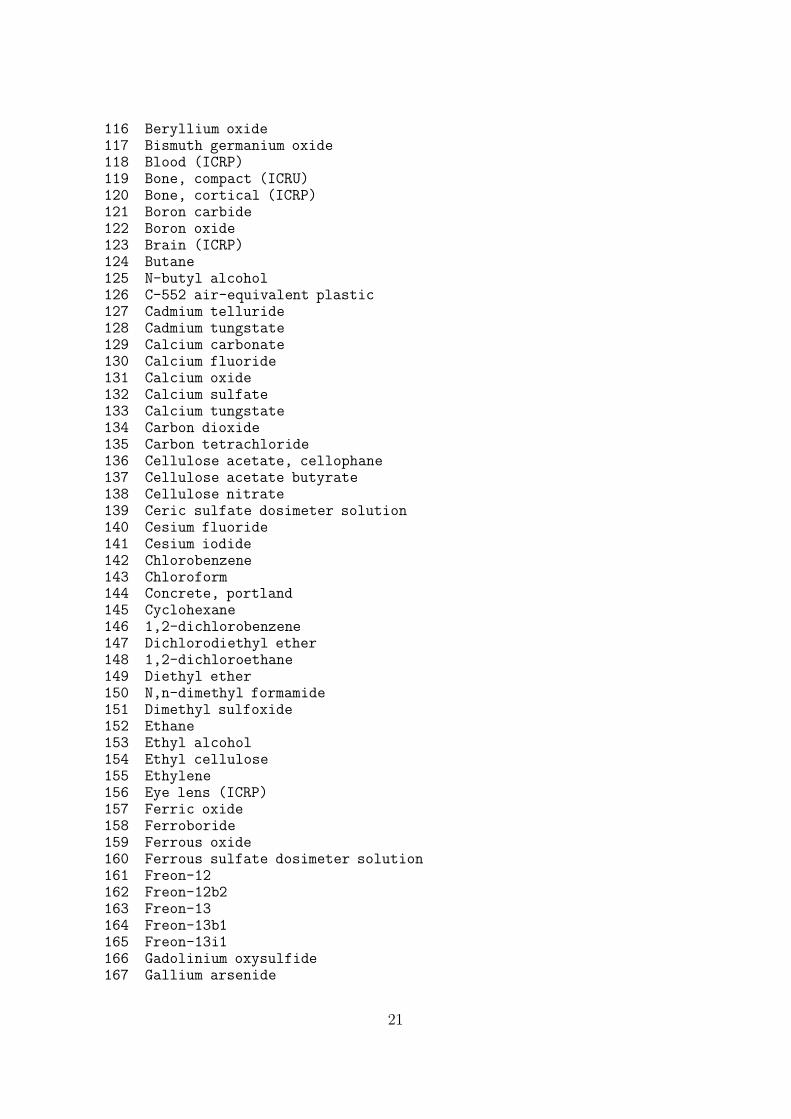
116 Beryllium oxide117 Bismuth germanium oxide118 Blood (ICRP)119 Bone, compact (ICRU)120 Bone, cortical (ICRP)121 Boron carbide122 Boron oxide123 Brain (ICRP)124 Butane125 N-butyl alcohol126 C-552 air-equivalent plastic127 Cadmium telluride128 Cadmium tungstate129 Calcium carbonate130 Calcium fluoride131 Calcium oxide132 Calcium sulfate133 Calcium tungstate134 Carbon dioxide135 Carbon tetrachloride136 Cellulose acetate, cellophane137 Cellulose acetate butyrate138 Cellulose nitrate139 Ceric sulfate dosimeter solution140 Cesium fluoride141 Cesium iodide142 Chlorobenzene143 Chloroform144 Concrete, portland145 Cyclohexane146 1,2-dichlorobenzene147 Dichlorodiethyl ether148 1,2-dichloroethane149 Diethyl ether150 N,n-dimethyl formamide151 Dimethyl sulfoxide152 Ethane153 Ethyl alcohol154 Ethyl cellulose155 Ethylene156 Eye lens (ICRP)157 Ferric oxide158 Ferroboride159 Ferrous oxide160 Ferrous sulfate dosimeter solution161 Freon-12162 Freon-12b2163 Freon-13164 Freon-13b1165 Freon-13i1166 Gadolinium oxysulfide167 Gallium arsenide

21

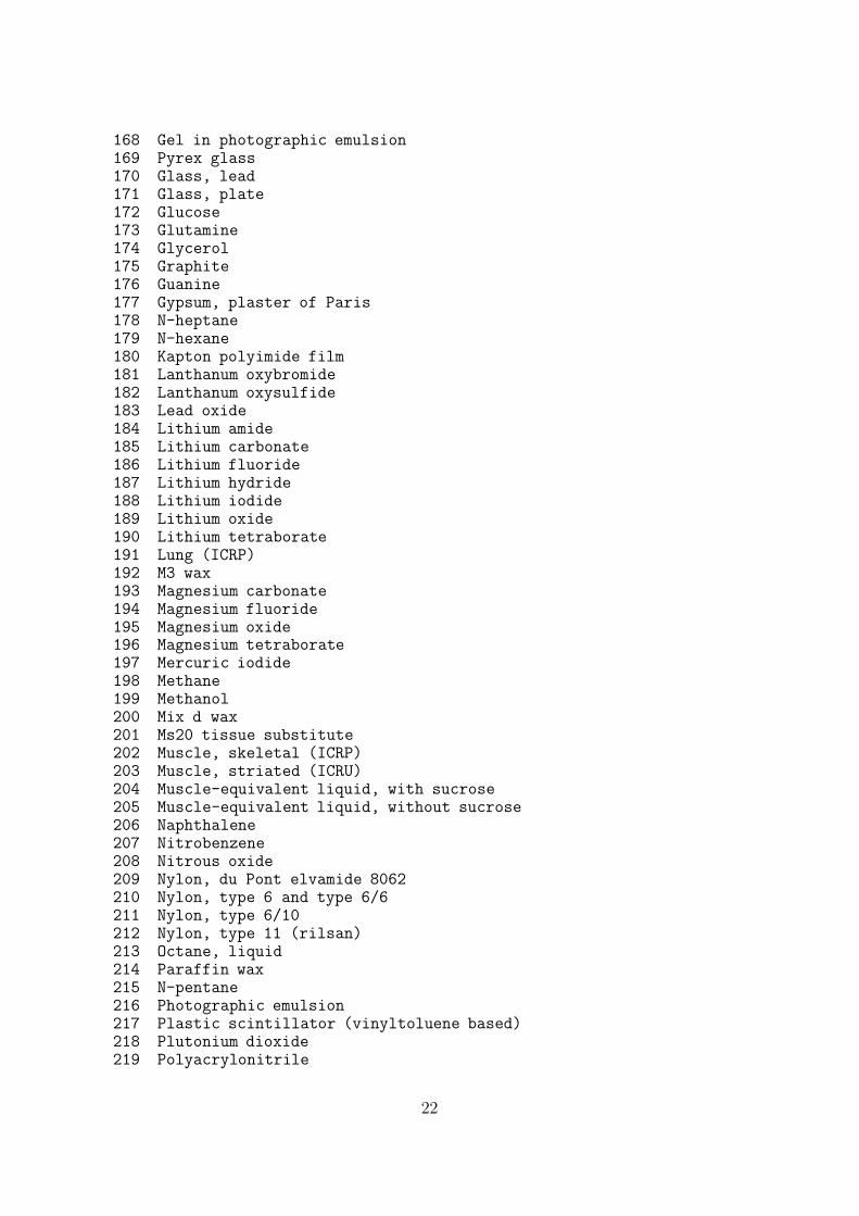
168 Gel in photographic emulsion169 Pyrex glass170 Glass, lead171 Glass, plate172 Glucose173 Glutamine174 Glycerol175 Graphite176 Guanine177 Gypsum, plaster of Paris178 N-heptane179 N-hexane180 Kapton polyimide film181 Lanthanum oxybromide182 Lanthanum oxysulfide183 Lead oxide184 Lithium amide185 Lithium carbonate186 Lithium fluoride187 Lithium hydride188 Lithium iodide189 Lithium oxide190 Lithium tetraborate191 Lung (ICRP)192 M3 wax193 Magnesium carbonate194 Magnesium fluoride195 Magnesium oxide196 Magnesium tetraborate197 Mercuric iodide198 Methane199 Methanol200 Mix d wax201 Ms20 tissue substitute202 Muscle, skeletal (ICRP)203 Muscle, striated (ICRU)204 Muscle-equivalent liquid, with sucrose205 Muscle-equivalent liquid, without sucrose206 Naphthalene207 Nitrobenzene208 Nitrous oxide209 Nylon, du Pont elvamide 8062210 Nylon, type 6 and type 6/6211 Nylon, type 6/10212 Nylon, type 11 (rilsan)213 Octane, liquid214 Paraffin wax215 N-pentane216 Photographic emulsion217 Plastic scintillator (vinyltoluene based)218 Plutonium dioxide219 Polyacrylonitrile

22

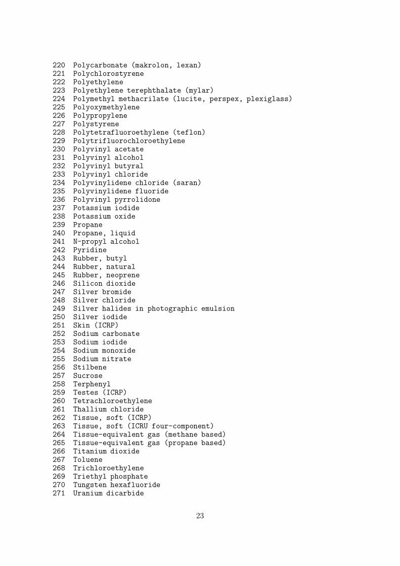
220 Polycarbonate (makrolon, lexan)221 Polychlorostyrene222 Polyethylene223 Polyethylene terephthalate (mylar)224 Polymethyl methacrilate (lucite, perspex, plexiglass)225 Polyoxymethylene226 Polypropylene227 Polystyrene228 Polytetrafluoroethylene (teflon)229 Polytrifluorochloroethylene230 Polyvinyl acetate231 Polyvinyl alcohol232 Polyvinyl butyral233 Polyvinyl chloride234 Polyvinylidene chloride (saran)235 Polyvinylidene fluoride236 Polyvinyl pyrrolidone237 Potassium iodide238 Potassium oxide239 Propane240 Propane, liquid241 N-propyl alcohol242 Pyridine243 Rubber, butyl244 Rubber, natural245 Rubber, neoprene246 Silicon dioxide247 Silver bromide248 Silver chloride249 Silver halides in photographic emulsion250 Silver iodide251 Skin (ICRP)252 Sodium carbonate253 Sodium iodide254 Sodium monoxide255 Sodium nitrate256 Stilbene257 Sucrose258 Terphenyl259 Testes (ICRP)260 Tetrachloroethylene261 Thallium chloride262 Tissue, soft (ICRP)263 Tissue, soft (ICRU four-component)264 Tissue-equivalent gas (methane based)265 Tissue-equivalent gas (propane based)266 Titanium dioxide267 Toluene268 Trichloroethylene269 Triethyl phosphate270 Tungsten hexafluoride271 Uranium dicarbide

23

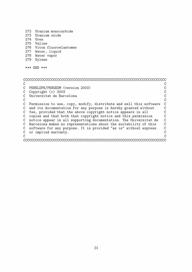
272 Uranium monocarbide273 Uranium oxide274 Urea275 Valine276 Viton fluoroelastomer277 Water, liquid278 Water vapor279 Xylene

*** END ***

CCCCCCCCCCCCCCCCCCCCCCCCCCCCCCCCCCCCCCCCCCCCCCCCCCCCCCCCCCCCCCCCCCCCCCCCC CC PENELOPE/PENGEOM (version 2003) CC Copyright (c) 2003 CC Universitat de Barcelona CC CC Permission to use, copy, modify, distribute and sell this software CC and its documentation for any purpose is hereby granted without CC fee, provided that the above copyright notice appears in all CC copies and that both that copyright notice and this permission CC notice appear in all supporting documentation. The Universitat de CC Barcelona makes no representations about the suitability of this CC software for any purpose. It is provided "as is" without express CC or implied warranty. CC CCCCCCCCCCCCCCCCCCCCCCCCCCCCCCCCCCCCCCCCCCCCCCCCCCCCCCCCCCCCCCCCCCCCCCCCC

24