1

FATIGUE LIFE PREDICTION OF THERMO-MECHANICALLY LOADED

ENGINE COMPONENTS

Csaba Halászi, Christian Gaier, Helmut Dannbauer

MAGNA Powertrain, Engineering Center Steyr GmbH & Co. KG

Steyrer str. 32, A-4300 St.Valentin, Austria

Keywords: thermo-mechanical fatigue, engine, Sehitoglu

INTRODUCTION

Nowadays engine components are subjected to higher loads at elevated temperatures than before,

due to the increasing requirements regarding weight, performance and exhaust gas emission. Thus,

fatigue due to simultaneous thermal and mechanical loading became determinant among the

damage forms.

At the same time, there is the need to reduce development times and costs to handle the growing

number of model variants. Therefore, the development of suitable simulation tools, which reduce

the number of necessary component tests, seems to be very rewarding.

The problem of thermo-mechanical fatigue (TMF) life prediction has received considerable

attention in recent years, with efforts principally concentrated on the prediction of TMF under

uniformly repeated loading conditions. Several researchers have developed models to treat this

problem, generally based on isothermal (IT) considerations. However, isothermal tests do not

capture all damage mechanisms that operate under variable strain-temperature conditions. As

Sehitoglu emphasizes, a deeper understanding of the different micro mechanisms affecting the

behavior of materials under isothermal and thermo-mechanical loading conditions is needed.

THERMO-MECHANICAL FATIGUE

Thermo-mechanical fatigue (TMF) is the case of fatigue failure due to simultaneous thermal and

mechanical loading. The life prediction of TMF loading cases has received considerable attention in

recent years mainly in engine and gas turbine development. The fluctuation of complex thermal and

mechanical strains is usually determinant for fatigue life of machine parts. The mechanical strain

arises either from external constraints or externally applied loadings.

Thermo-mechanical and low cycle fatigue (LCF) can show a lot of similarity, mainly because of

the presence of cyclic plastic strain. The cyclic thermal load occurs by nature in a small number of

cycles, but the stresses generated by the restrained thermal expansion may be far beyond the elastic

limit. In engine parts the superposition of a LCF/TMF effect due to start-stop cycles and a HCF

effect due to the combustion cycle is to be observed.

Throughout a thermo-mechanical cycle, one crosses different temperatures. The temperature

dependent processes that occur during a common TMF cycle are plastic deformation, cyclic aging,

2

creep and oxidation effects, coarsening of the microstructure and crack initiation and propagation.

The main damage mechanisms are fatigue (mechanical) damage, environmental (oxidation) damage

and creep damage. These may act independently or can interact depending on various material

characteristics like thermal conductivity, thermal strain coefficient, Young’s modulus, mechanical

properties and operating conditions, as maximum and minimum temperatures, mechanical strain

range, strain rate, phasing of temperature and mechanical strain, dwell time, environmental factor.

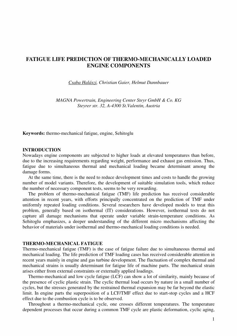
TMF testing methodology

In TMF tests a specimen is subjected to a desired thermal and mechanical strain with different

phasings. Two baselines of TMF tests are conducted in the laboratory with proportional phasings:

in-phase (IP), where the maximum strain (the strain is signed: tension has a positive, and

compression has a negative sign) occurs at maximum temperature, and out-of-phase (OP), with

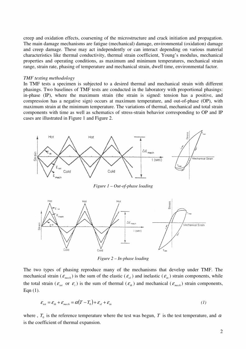
maximum strain at the minimum temperature. The variations of thermal, mechanical and total strain

components with time as well as schematics of stress-strain behavior corresponding to OP and IP

cases are illustrated in Figure 1 and Figure 2.

Figure 1 – Out-of-phase loading

Figure 2 – In-phase loading

The two types of phasing reproduce many of the mechanisms that develop under TMF. The

mechanical strain ( mechε ) is the sum of the elastic ( elε ) and inelastic ( inε ) strain components, while

the total strain ( totε or tε ) is the sum of thermal ( thε ) and mechanical ( mechε ) strain components,

Eqn (1).

( ) inelmechthtot TT εεαεεε ++−=+= 0 (1)

where , 0T is the reference temperature where the test was begun, T is the test temperature, and α

is the coefficient of thermal expansion.

3

SEHITOGLU’S TMF LIFE PREDICTION MODEL

Prof. Huseyin Sehitoglu and his colleagues at the University of Illinois, Urbana-Champaign

developed a method for life prediction of thermo-mechanically loaded components. This method

includes a unified constitutive visco-plastic material model to describe the material behavior at

different temperatures and strain rates in the stress-strain analysis, and a damage model.

The damage model is based on three separate damage mechanisms (fatigue, environmental

attack, creep) that are acting simultaneously. Depending on the strain rate, strain amplitude,

temperature and phasing these damage mechanisms can have different parts in the total damage,

which is the sum of these components. Formally:

creepoxfattot DDDD ++= or creepoxfattot

NNNN

1111++= (2)

where totD , fatD , oxD and creepD are total damage, fatigue (mechanical) damage, environmental

(oxidation) and creep damage, respectively, and totN , fat

N , oxN , creep

N are total cycles to failure,

cycles to failure due to mechanical fatigue, oxidation and creep damage, respectively.

Fatigue (mechanical) damage

Fatigue damage is represented by the classical fatigue mechanisms, which normally occur at

ambient temperature. These include crack nucleation and propagation due to the strain amplitude.

Since the cyclic plastic strain is remarkable, strain-life approach is used to describe the fatigue

behavior. The fatigue life term, fatN , is estimated with the Manson-Coffin-Basquin relationship:

( ) ( )cfat

f

bfatfpl

mech

e

mechmech NNE

2'2'

222ε

σεεε+=

∆+

∆=

∆ (3)

Tests performed with steel and aluminum showed that the room temperature (RT) strain-life curve

can be considered as an upper bound of all strain-life curves. Thus, the constants ( cbE ff ,,,, εσ ′′ ) are

determined from isothermal room-temperature fatigue tests. As the temperature increases, the

damage increases due to oxidation and creep.

Environmental (oxidation) damage

Oxidation damage mechanism includes crack nucleation in surface oxides and oxide-induced crack

growth. Crack nucleation is defined as the rupture of the first oxide layer. Oxide-induced crack

growth is described as the repeated formation of an oxide layer at the crack tip and its rupture,

exposing fresh metallic surface to the environment.

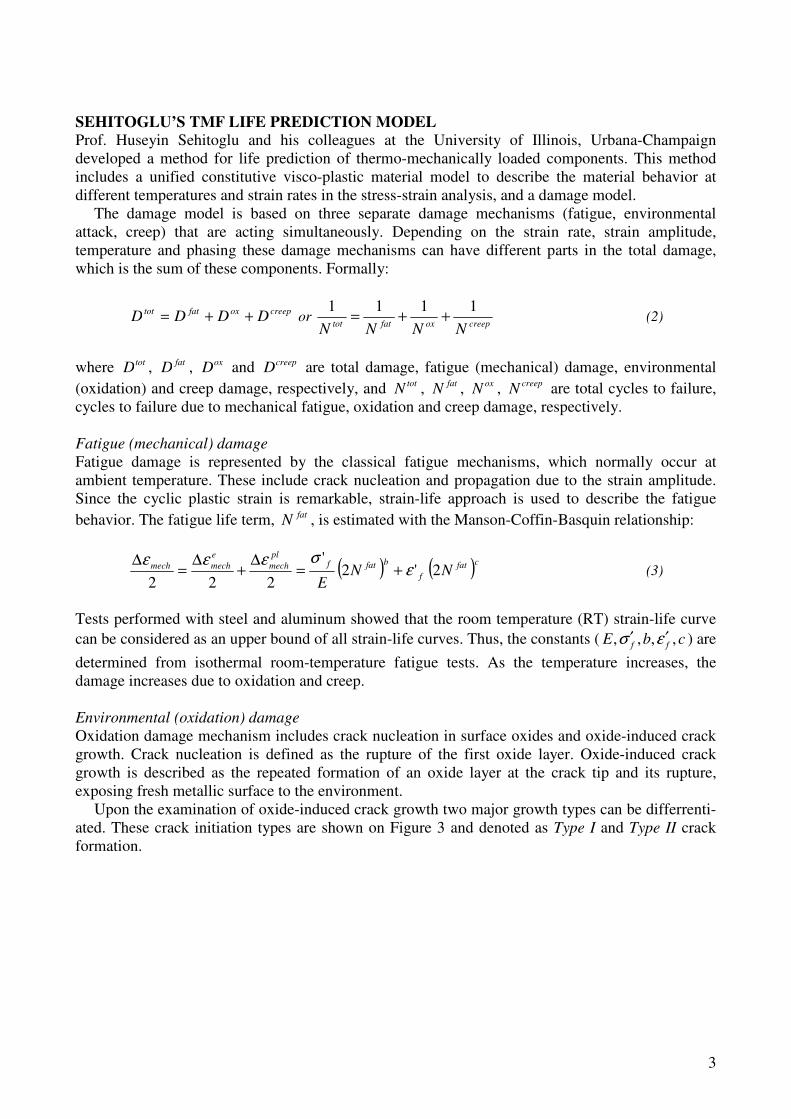
Upon the examination of oxide-induced crack growth two major growth types can be differrenti-

ated. These crack initiation types are shown on Figure 3 and denoted as Type I and Type II crack

formation.

4

Figure 3 – left: Type I growth, right: Type II growth

All oxide-induced crack growth process starts with an initial oxide layer formed on the surface of

the specimen. When this layer reaches a critical thickness, the oxide ruptures, and the crack

nucleation has occurred. Then a fresh metallic surface is exposed to the environment, which rapidly

oxidizes. When the thickness of this newly formed oxide reaches its own critical thickness, the

oxide ruptures again. The process continues as shown in Figure 3.

Type I growth is characterized by a “continuous” oxide layer. This layer results in oxide

intrusion without any visible stratification. Therefore, it will be distinguished from Type II, which is

characterized by “multilayered” or “stratificated” oxide growth. It is important to note, that the

progression of both growth types is similar until the layer reaches its critical thickness. The

difference comes up with the first rupture, as in Type II growth the oxide layer detaches from the

surface of the substrate. This results in exposition of a larger fresh surface area to the environment,

accounting for a wider intrusion,

The oxidation damage is calculated using following equation:

( )( )

( )β

ββ

ε

εδa

mech

mech

eff

p

ox

cr

ox

ox

KB

h

ND

−

+−

∆

Φ==

1

121

0 21

& (4)

where hcr, δ0, α, β and B are material parameters. mechε& is the mechanical strain rate and eff

pK is the

effective oxidation constant,

( )dt

tT

QD

tK

Ct

C

eff

p ∫

−=

0

0R

exp1

(5)

where D0 is a constant, Q is the activation energy for oxidation and R is the universal gas constant.

5

The Oxidation Phasing Factor

( )dt

tox

mechtht

c

ox c

+−=Φ ∫

2

0

1/

2

1exp

1

ξ

εε && (6)

where ξox measures the relative amount of damage associated with different phasing. thε& is the

thermal strain rate.

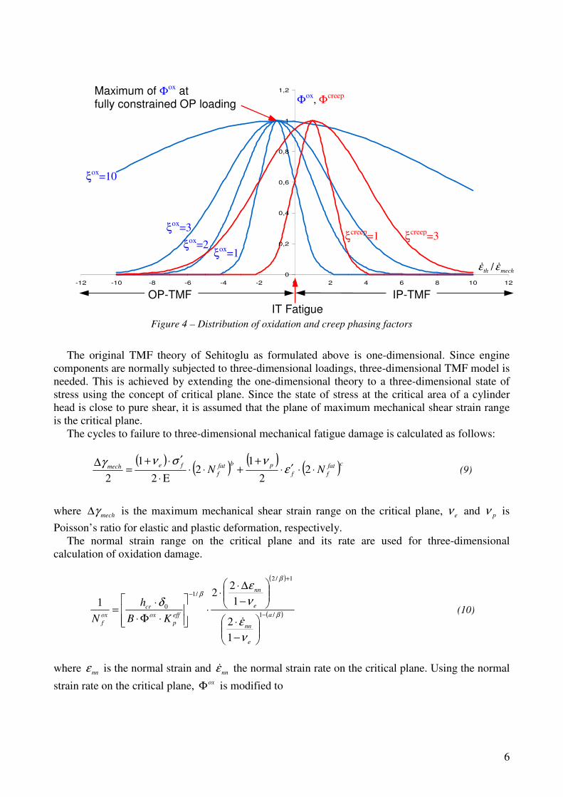
The form of oxΦ is chosen to represent the behavior of the oxidation damage observed in the

tests. The most detrimental TMF loading case is the fully constrained out-of-phase, which is

represented by the ratio ( )1/ −=mechth εε && . For the case of free expansion ( )±∞=mechth εε && / no

oxidation damage was observed, therefore oxΦ should approach zero. All other histories have a

unique value for oxΦ , which fall between these extremes.

Creep damage

Creep damage is observed in the form of internal intergranular cracking at the grain boundaries

perpendicular to the loading direction. Crack propagation continues until rapid crack growth

commences by linkup of these intergranular cracks, and make the specimen or component fracture.

The creep damage model is based on the integration of temperature, strain-temperature phasing

and stress history over time. This approach can handle the sensitivity of creep damage accumulation

for various conditions e.g. strain rate or different TMF phasings. Formally written:

( )∫

+

∆−Φ⋅=

Ctm

Heqcreepcreepdt

KtT

HAD

0

21

Rexp

σασα (7)

where eqσ is the equivalent stress, Hσ is the hydrostatic stress, K is the drag stress, creepΦ is the

creep phasing factor, A and m are material constants, and 1α and 2α are scaling factors. The test

specimens showed different creep damage for tension and compression, and the role of the scaling

factors 1α and 2α is to represent this asymmetry. The term H∆ describes the activation energy for

creep, and ( )tT is the temperature as a function of time.

To consider the influence of strain-temperature phasing, a creep phasing factor is introduced,

which is similar to the one used in the oxidation damage term. Formally:

( )dt

tcreep

mechth

t

c

creepc

−−=Φ ∫

2

0

1/

2

1exp

1

ξ

εε && (8)

The function creepΦ shows normal distribution characterizing the severity of creep damage for any

ratio of the thermal and mechanical strain rates. The constant creepξ defines the sensitivity of the

phasing to the creep damage. From laboratory tests, the in-phase TMF case ( 1/ =mechth εε && ) showed

the most creep damage, therefore this loading case is assigned the peak value 1=Φcreep .

6

0

0,2

0,4

0,6

0,8

1

1,2

-12 -10 -8 -6 -4 -2 0 2 4 6 8 10 12

Figure 4 – Distribution of oxidation and creep phasing factors

The original TMF theory of Sehitoglu as formulated above is one-dimensional. Since engine

components are normally subjected to three-dimensional loadings, three-dimensional TMF model is

needed. This is achieved by extending the one-dimensional theory to a three-dimensional state of

stress using the concept of critical plane. Since the state of stress at the critical area of a cylinder

head is close to pure shear, it is assumed that the plane of maximum mechanical shear strain range

is the critical plane.

The cycles to failure to three-dimensional mechanical fatigue damage is calculated as follows:

( ) ( ) ( ) ( )cfat

ff

pbfat

f

femech NN ⋅⋅′⋅+

+⋅⋅⋅

′⋅+=

∆2

2

12

E2

1

2ε

νσνγ (9)

where mechγ∆ is the maximum mechanical shear strain range on the critical plane, eν and pν is

Poisson’s ratio for elastic and plastic deformation, respectively.

The normal strain range on the critical plane and its rate are used for three-dimensional

calculation of oxidation damage.

( )

( )β

β

β

ν

ε

ν

ε

δ/1

1/2

/1

0

1

2

1

22

1a

e

nn

e

nn

eff

p

ox

cr

ox

f KB

h

N−

+

−

−

⋅

−

∆⋅⋅

⋅

⋅Φ⋅

⋅=

&

(10)

where nnε is the normal strain and nnε& the normal strain rate on the critical plane. Using the normal

strain rate on the critical plane, oxΦ is modified to

mechth εε && /

IT Fatigue

IP-TMF OP-TMF

Maximum of Φox at fully constrained OP loading Φox

, Φcreep

ξox=10

ξox=3

ξox=2

ξox=1

ξcreep=3 ξcreep

=1

7

( )

dtt

ct

ox

nn

the

c

ox

∫

+

⋅

⋅−

⋅−=Φ0

2

12

1

2

1exp

1

ξ

ε

εν

&

&

(11)

Since creep damage is based on stress invariants, Equation 7 is three-dimensional. creepΦ is

calculated using normal strain and normal strain rate on the critical plane

( )

dtt

ct

creep

nn

the

c

creep

∫

−

⋅

⋅−

⋅−=Φ0

2

12

1

2

1exp

1

ξ

ε

εν

&

&

(12)

DETERMINATION OF THE MATERIAL PARAMETERS FOR SEHITOGLU’S TMF

MODEL

Sehitoglu’s TMF life prediction model involves several material parameters which can only be

determined by special and usually expensive and time-consuming tests and measurements. In ECS

an alternative way was developed to determine these parameters using conventional isothermal LCF

and TMF test results. The method is based on parameter identification using evolutionary

algorithms like Evolution Strategy (ES) and Differential Evolution (DE). Above all the DE method

proved to be the most suitable for this problem because of its better convergence and less

computation time. The algorithms were implemented in user friendly software with GUI using

Maple.

Parameter optimization

The definition of the parameter optimization (also denoted as parameter identification) is as

follows: an objective function ( ) ℜ→ℜnf :x is given, whose – scalar – value depends on n

independent parameters nxx ,...,1 , which formulate a parameter vector x . The goal is to find over

the set 0/≠M a special vector M∈*x , which satisfies the following:

**)()(: fffM =≥∈∀ xxx (13)

Hence the value *f is called the global optimum, and the vector *x is the minimum location

(point or set).

Our objective function is based on the familiar least square fitting problem

( ){ }xfmin , where ( ) ( )[ ]∑=

−=m

i

ilii ppyyf1

2

,1 ,..., xx (14)

iy is the dependent variable (output), and ( )ili pp ,...,1 are the independent variables (input) to the

objective function.

8

Since fatigue tests are usually performed in several orders of magnitude, the use of the objective

function described above would hugely overestimate the failures, when the number of cycles is

great. Therefore, it seems to be practical to use the natural logarithm of the dependent variable:

( ) [ ] ∑∑==

=−=

m

ie

i

c

im

i

e

i

c

iN

NNNf

1

2

1

2lnlnlnx (15)

where c

iN is the calculated fatigue life and e

iN is the experimental fatigue life.

Strain rate can be given with strain range and cycle time, Cmechmech tεε ∆= 2& . Using this

relationship and joining together the three damage mechanisms the required independent variables

are

• Mechanical strain range mechε∆

• Young’s modulus E

• Temperature history ( )tT over the cycle time Ct

• Phasing history ( ) ( )tt mechth εε && over cycle time Ct

• Equivalent and hydrostatic stress history ( )teqσ and ( )tHσ over cycle time Ct

• An approximation of drag stress as a function of temperature ( )TK

Let’s start the definition of the parameters with two simplifications: first, the oxidation damage

term given in Eqn. (3) contains the parameters Bhcr ,, 0δ and 0D in eff

pK , which remain constant

over time. Mathematically seen they can be replaced with one constant

0

0

DB

hC cr

⋅

⋅=

δ (16)

Second the parameters 21 ,, ααA in the creep damage term are not independent from each other,

i.e. if all other variables are identical ( ) ( )( )mmmnAnnA 2121 ,, αααα ⋅=⋅⋅⋅ holds, giving different

results to all three values. Investigating only A and the ratio 21 αα solves this problem. Setting

12 =α reduces our optimization problem for searching only A and 1α .

Hereafter the three damage terms form the following parameter vectors

• Mechanical damage uses ( )cb ff ,',,' εσ

• Oxidation damage uses ( )oxCQa ξβ ,,,,

• Creep damage uses ( )crmHA ξα ,,,, 1∆

Evolution Strategies

The idea to use principles of organic evolution processes as rules for optimum seeking procedures

emerged in the USA and in Europe independently nearly four decades ago. Both approaches rely

upon imitating the natural selection described by Darwin in his framework „The Origin of Species”

in 1859.

These algorithms rely on the concept of a population of individuals (representing potential

solutions to a given optimization problem), which undergo probabilistic operators, such as

mutation, selection, and (sometimes) recombination to evolve towards increasingly better fitness

values of individuals. The fitness of an individual reflects its value with respect to a particular

objective function to be optimized. The main loop of the algorithm, consisting of recombination,

9

mutation, fitness evaluation and selection is iterated for a number of generations until the

computing time is exhausted, a sufficiently good solution is found, or some other termination

criterion is fulfilled.

All evolutionary algorithms cope with a group of possible solutions called population. Parents

denote the members of the population that serves as the generator of a subsequent population of

individuals called offsprings. Every time a new set of offsprings is spawned, the evolution process

advances one generation.

The initialisation is usually carried out by picking a defined number of individuals at random

from the search space.

The recombination operator allows us to create new individuals based on the members of the

previous generation. The main idea behind recombination was that it should help to avoid

unsuitable values for the individuals – mainly to the strategy parameters – by mixing the

information coded in the parents and hereby reduce the time/number of generations to reach the

optimum.

The mutation of the strategy parameters plays an important role in fitting the population to the

topological characteristics of the objective function. In the early phase of the optimization the

deviations should be large enough to scan the surface of the objective function. As soon as the

strategy finds an optimum, the deviations should decrease to lower the diversity of the population.

The mutation of the strategy parameters takes place according to some learning rules, which

make the algorithm possible to fit the deviations automatically. This process is called self-

adaptation.

Selection is the heart of evolution. Without selection, ES would perform a random walk due to

the random movements generated by the mutation operator. The selection gives the ‘direction’ to

the process by preferring the better individuals to survive, providing an active driving force for

improvement.

In order to stop the evolutionary process and accept the best found individual as the solution of

the optimization problem, one or several termination criteria have to be established. The most

widely used criteria are as follows:

1. maximum number of generations or function evaluations

2. minimum value of the fitness function

3. maximum number of generations without improvement

4. minimum threshold of the improvement in the fitness value in a certain number of

generations

All of these termination criteria have their advantages and drawbacks. Usually a combination of

these termination criteria (e.g. 1+2, or 2+4) is used in many applications.

FATIGUE LIFE PREDICTION OF A DIESEL PISTON

In this chapter the process of a TMF simulation will be presented based on a simple example of a

diesel piston.

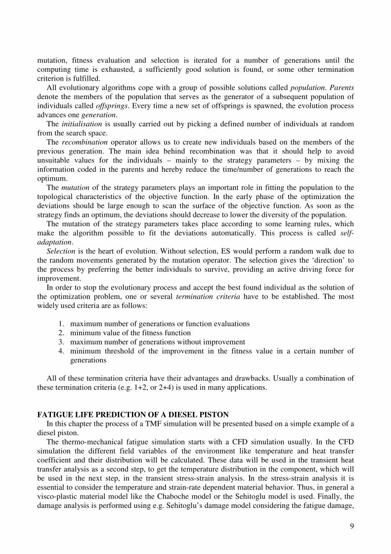
The thermo-mechanical fatigue simulation starts with a CFD simulation usually. In the CFD

simulation the different field variables of the environment like temperature and heat transfer

coefficient and their distribution will be calculated. These data will be used in the transient heat

transfer analysis as a second step, to get the temperature distribution in the component, which will

be used in the next step, in the transient stress-strain analysis. In the stress-strain analysis it is

essential to consider the temperature and strain-rate dependent material behavior. Thus, in general a

visco-plastic material model like the Chaboche model or the Sehitoglu model is used. Finally, the

damage analysis is performed using e.g. Sehitoglu’s damage model considering the fatigue damage,

10

environmental damage and creep damage. The process of the TMF simulation can be seen in the

next Figure.

Figure 5 – TMF simulation process

Heat transfer analysis

Since it was a test example, the CFD analysis was omitted. The temperature distribution of the oil

film and the gas were estimated based on experimental data. The material is a typical piston

aluminum cast alloy GK-AlSi12CuMgNi.

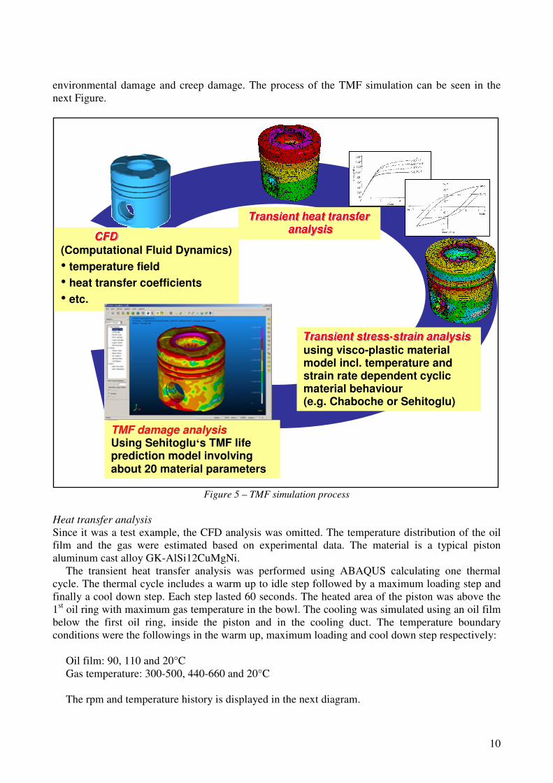
The transient heat transfer analysis was performed using ABAQUS calculating one thermal

cycle. The thermal cycle includes a warm up to idle step followed by a maximum loading step and

finally a cool down step. Each step lasted 60 seconds. The heated area of the piston was above the

1st oil ring with maximum gas temperature in the bowl. The cooling was simulated using an oil film

below the first oil ring, inside the piston and in the cooling duct. The temperature boundary

conditions were the followings in the warm up, maximum loading and cool down step respectively:

Oil film: 90, 110 and 20°C

Gas temperature: 300-500, 440-660 and 20°C

The rpm and temperature history is displayed in the next diagram.

TTTrrraaannnsssiiieeennnttt hhheeeaaattt tttrrraaannnsssfffeeerrr

aaannnaaalllyyysssiiisss CCCFFFDDD

(Computational Fluid Dynamics)

• temperature field

• heat transfer coefficients

• etc.

TTTrrraaannnsssiiieeennnttt ssstttrrreeessssss---ssstttrrraaaiiinnn aaannnaaalllyyysssiiisss using visco-plastic material model incl. temperature and strain rate dependent cyclic material behaviour (e.g. Chaboche or Sehitoglu)

TTMMFF ddaammaaggee aannaallyyssiiss Using Sehitoglu‘s TMF life prediction model involving about 20 material parameters

11

Figure 6 – RPM and temperature history

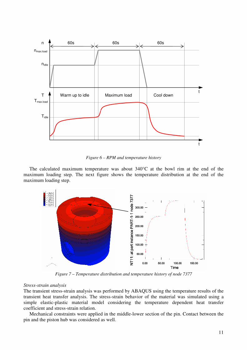
The calculated maximum temperature was about 340°C at the bowl rim at the end of the

maximum loading step. The next figure shows the temperature distribution at the end of the

maximum loading step.

Figure 7 – Temperature distribution and temperature history of node 7377

Stress-strain analysis

The transient stress-strain analysis was performed by ABAQUS using the temperature results of the

transient heat transfer analysis. The stress-strain behavior of the material was simulated using a

simple elastic-plastic material model considering the temperature dependent heat transfer

coefficient and stress-strain relation.

Mechanical constraints were applied in the middle-lower section of the pin. Contact between the

pin and the piston hub was considered as well.

n

T

nidle

nmax.load

Tmax.load

Tidle

Warm up to idle Maximum load Cool down

60s 60s 60s

t

t

12

Pressure distribution was applied above the 1st oil ring for each time increment to simulate the

operational combustion pressure. Neither side nor mass force was considered.

The Mises stress distribution at maximum loading is shown in the next figure.

Figure 8 – Mises stress distribution and Mises stress history of node 7377

Damage analysis

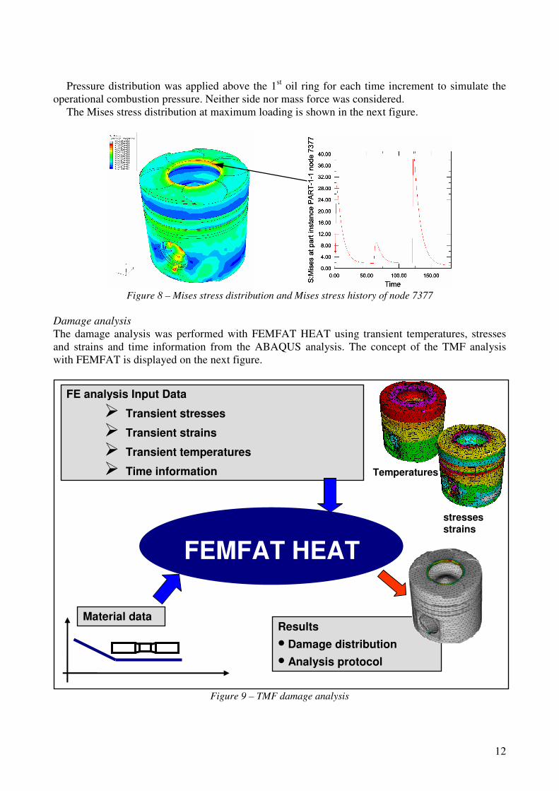
The damage analysis was performed with FEMFAT HEAT using transient temperatures, stresses

and strains and time information from the ABAQUS analysis. The concept of the TMF analysis

with FEMFAT is displayed on the next figure.

Figure 9 – TMF damage analysis

Results

• Damage distribution

• Analysis protocol

FE analysis Input Data

� Transient stresses

� Transient strains

� Transient temperatures

� Time information

Material data

FEMFAT HEAT

Temperatures

stresses strains

13

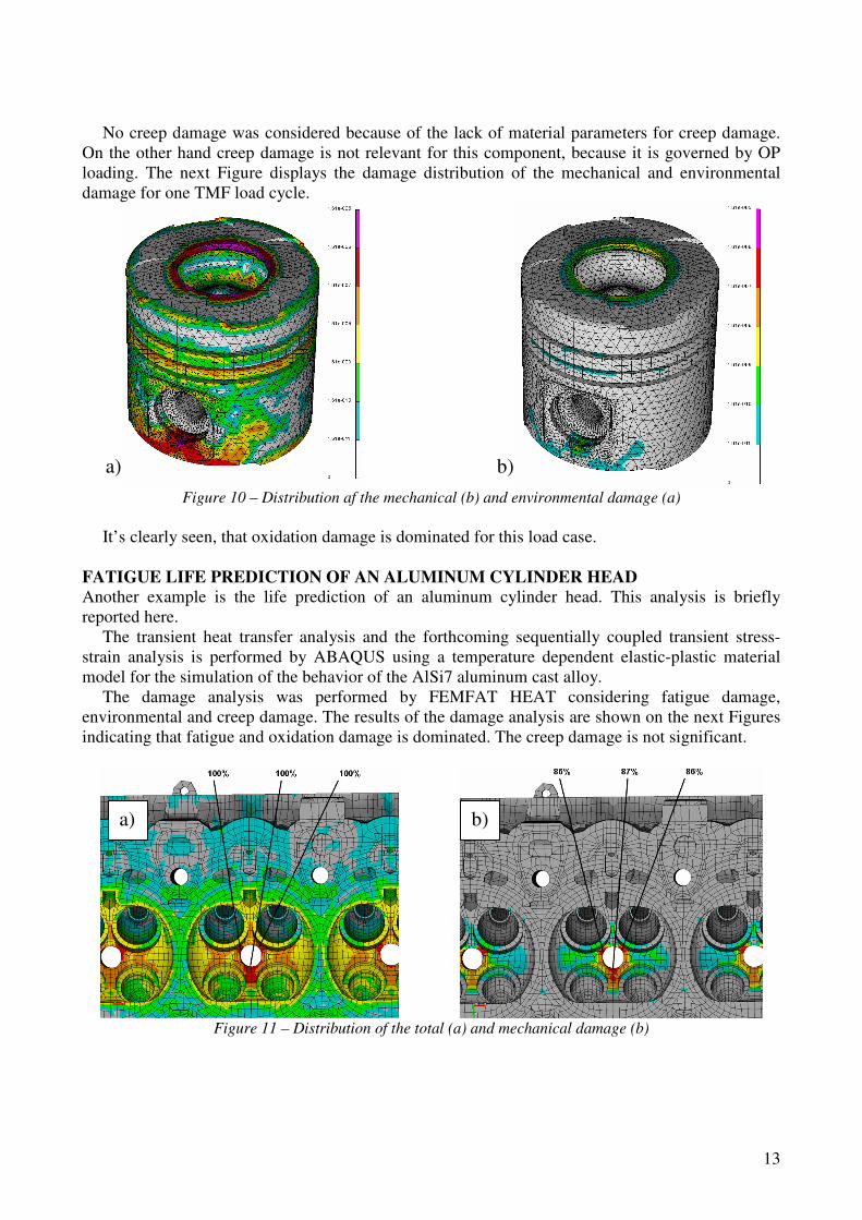
No creep damage was considered because of the lack of material parameters for creep damage.

On the other hand creep damage is not relevant for this component, because it is governed by OP

loading. The next Figure displays the damage distribution of the mechanical and environmental

damage for one TMF load cycle.

Figure 10 – Distribution af the mechanical (b) and environmental damage (a)

It’s clearly seen, that oxidation damage is dominated for this load case.

FATIGUE LIFE PREDICTION OF AN ALUMINUM CYLINDER HEAD

Another example is the life prediction of an aluminum cylinder head. This analysis is briefly

reported here.

The transient heat transfer analysis and the forthcoming sequentially coupled transient stress-

strain analysis is performed by ABAQUS using a temperature dependent elastic-plastic material

model for the simulation of the behavior of the AlSi7 aluminum cast alloy.

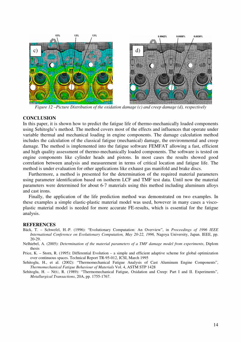
The damage analysis was performed by FEMFAT HEAT considering fatigue damage,

environmental and creep damage. The results of the damage analysis are shown on the next Figures

indicating that fatigue and oxidation damage is dominated. The creep damage is not significant.

Figure 11 – Distribution of the total (a) and mechanical damage (b)

a) b)

a) b)

14

Figure 12 –Picture Distribution of the oxidation damage (c) and creep damage (d), respectively

CONCLUSION

In this paper, it is shown how to predict the fatigue life of thermo-mechanically loaded components

using Sehitoglu’s method. The method covers most of the effects and influences that operate under

variable thermal and mechanical loading in engine components. The damage calculation method

includes the calculation of the classical fatigue (mechanical) damage, the environmental and creep

damage. The method is implemented into the fatigue software FEMFAT allowing a fast, efficient

and high quality assessment of thermo-mechanically loaded components. The software is tested on

engine components like cylinder heads and pistons. In most cases the results showed good

correlation between analysis and measurement in terms of critical location and fatigue life. The

method is under evaluation for other applications like exhaust gas manifold and brake discs.

Furthermore, a method is presented for the determination of the required material parameters

using parameter identification based on isotherm LCF and TMF test data. Until now the material

parameters were determined for about 6-7 materials using this method including aluminum alloys

and cast irons.

Finally, the application of the life prediction method was demonstrated on two examples. In

these examples a simple elastic-plastic material model was used, however in many cases a visco-

plastic material model is needed for more accurate FE-results, which is essential for the fatigue

analysis.

REFERENCES Bäck, T. – Schwefel, H.-P. (1996): “Evolutionary Computation: An Overview”, in Proceedings of 1996 IEEE

International Conference on Evolutionary Computation, May 20-22, 1996, Nagoya University, Japan. IEEE, pp.

20-29.

Nelhiebel, A. (2005): Determination of the material parameters of a TMF damage model from experiments, Diplom

thesis

Price, K. – Storn, R. (1995): Differential Evolution – a simple and efficient adaptive scheme for global optimization

over continuous spaces. Technical Report TR-95-012, ICSI, March 1995

Sehitoglu, H., et al. (2002): “Thermomechanical Fatigue Analysis of Cast Aluminum Engine Components”,

Thermomechanical Fatigue Behaviour of Materials Vol. 4, ASTM STP 1428

Sehitoglu, H. – NEU, R. (1989): “Thermomechanical Fatigue, Oxidation and Creep: Part I and II. Experiments”,

Metallurgical Transactions, 20A, pp. 1755-1767.

c) d)