


Languages
Pages
Legal

FACTORS CONTRIBUTING TO THE FORMATION
OF SHEETING JOINTS: A STUDY OF SHEETING JOINTS ON A DOME IN
YOSEMITE NATIONAL PARK
A THESIS SUBMITTED TO THE GRADUATE DIVISION OF THE
UNIVERSITY OF HAWAI„I AT MĀNOA IN PARTIAL FULFILLMENT
OF THE REQUIREMENTS FOR THE DEGREE OF
MASTERS OF SCIENCE
IN
GEOLOGY AND GEOPHYSICS
AUGUST 2010
By
Kelly J. Mitchell
Thesis Committee:
Steve Martel, Chairperson
Fred Duennebier
Paul Wessel
Keywords: sheeting joints, exfoliation joints, topographic stresses,
curvature, mechanics, spectral filtering, Yosemite

ii
Acknowledgements
I would like to extend my sincerest gratitude to those who helped make this thesis
possible. Thanks to the National Science Foundation for funding this research. Thank
you to my graduate advisor, Dr. Steve Martel, for your advice and support through the
past few years. This has been a long and difficult project but you have been patient and
supportive through it all. Special thanks to my committee, Dr. Fred Duennebier and Dr.
Paul Wessel for their advice and contributions; without your help I do not think this
project would have been possible. I appreciate the time all of you have spent discussing
the project with me. Thank you to Chris Hurren, Shay Chapman, and Carolyn Parcheta
for your hard work and moral support in the field; you kept a great attitude during the
field season. Special thanks to the National Park Service staff in Yosemite, particularly
Dr. Greg Stock and Brian Huggett for their assistance. I wish to thank NCALM, Ole
Kaven, Nicholas VanDerElst, and Emily Brodsky for LIDAR data collection. Thank you
to Carolina Anchietta Fermin, Lisa Swinnard, and Darwina Griffin for their moral
support. Finally, I want to express my deep gratitude to my family for their love and
encouragement. Mom, Dad, and Ryan, I love you. Thank you for your patience and
emotional support.
iii
Abstract
Sheeting joints (shallow, surface-parallel, opening-mode rock fractures) are widespread
and have been studied for centuries. They are commonly attributed to removal of
overburden by erosion, but erosion alone cannot open a sheeting joint. I test an
alternative hypothesis that sheeting joints open in response to surface-parallel
compression along a convex topographic surface using field observations, a large-
scale fracture map, and analyses of stresses, slopes, and surface-curvatures (derived from
aerial laser altimetry data) for a dome along Tenaya Creek in Yosemite National Park.
Approximately 90% of the surface of detailed study is convex in at least one direction.
Existing stresses and topography there can account for the nature and distribution of
sheeting joints on the doubly-convex surfaces. Sheeting joints parallel and constitute the
surface where the surface is doubly convex. Elsewhere, sheeting joints daylight,
implying the surface has been eroded since the sheeting joints formed. My findings
support the hypothesis.
iv
Table of Contents
Acknowledgements ........................................................................................................... ii
Abstract ............................................................................................................................. iii
List of Tables ................................................................................................................... vii
List of Figures ................................................................................................................. viii
Chapter 1. Introduction ....................................................................................................1
1.1 Motivation ..................................................................................................................1
1.2 Characteristics of sheeting joints ................................................................................2
1.3 Previous work .............................................................................................................3
1.4 Hypothesis to be tested ...............................................................................................7
1.5 Study area ...................................................................................................................7
1.6 Outline ........................................................................................................................8
Chapter 2. Mechanical Hypothesis ...................................................................................9
Chapter 3. Curvature Tutorial .......................................................................................16
3.1 Curvature of a plane curve .......................................................................................16
3.2 Curvature of surfaces ...............................................................................................18
Chapter 4. Geology ..........................................................................................................22
4.1 Geologic overview of the Tenaya Lake region ........................................................22
4.2 Sheeting joints of the Tenaya Lake region ...............................................................23
4.2.1 Characteristics ...................................................................................................24
4.2.2 Age ....................................................................................................................25
4.3 Geologic structures of the TC Dome study area ......................................................26
4.3.1 Structural features older than the sheeting joints ..............................................27
v
4.3.2 Sheeting joints ...................................................................................................28
4.3.3 Structural features younger than the sheeting joints ..........................................30
Chapter 5. Aerial LIDAR Data.......................................................................................32
5.1 Data collection ..........................................................................................................32
5.2 Calibration and point cloud data ..............................................................................33
5.3 Filtering and gridding by NCALM ..........................................................................34
Chapter 6. Stresses and Topographic Analyses ............................................................36
6.1 Stresses .....................................................................................................................36
6.2 Curvature of an ellipsoidal surface ...........................................................................38
6.3 Analyses of unsmoothed topographic data ...............................................................39
6.4 Spectral filtering .......................................................................................................39
6.5 Topographic geometry of filtered data .....................................................................41
6.6 Stress gradient analyses ............................................................................................45
Chapter 7. Discussion and Conclusions .........................................................................48
7.1 Scale of sheeting joints and topography ...................................................................48
7.2 Modern conditions for sheeting joint nucleation at TC Dome study area ...............49
7.3 Stress gradient and the distribution and nature of sheeting joints at TC Dome .......51
7.4 Other lessons ............................................................................................................55
7.5 Suggestions for future work .....................................................................................55
7.6 Conclusions ..............................................................................................................57
Figures ...............................................................................................................................60

vi
Appendix A. Orientation of Structural Features at TC Dome ..................................101
Appendix B. Curvature of Individual Sheeting Joints ...............................................104
References Cited.............................................................................................................108

vii
List of Tables
1. Topographic shapes based on principal curvature ...................................................13
2. Topographic shapes based on mean and Gaussian curvature .................................20
3. Orientation of Group F fractures ...............................................................................28
viii
List of Figures
1. Sheeting joints at Shuteye Peak, California ..............................................................60
2. Sheeting joints in cross-section ...................................................................................60
3. Tioga Quarry ................................................................................................................61
4. Map of Yosemite and Tenaya Lake study region .....................................................61
5. Shaded relief map of Tenaya Lake study region.......................................................62
6. Shaded relief map of TC Dome study area ................................................................63
7. Free body diagram .......................................................................................................64
8. Circular arc diagram ...................................................................................................64
9. Principal curvatures of a saddle-shaped surface ......................................................65
10. Curvature of a bell-shaped hill .................................................................................65
11. Heavily eroded sheeting joints ..................................................................................66
12. Groundwater seeping from sheeting joints..............................................................67
13. Hackle marks ..............................................................................................................68
14. Lack of slip across sheeting joint faces ....................................................................69
15. TC Dome as seen from Tenaya Creek......................................................................69
16. TC Dome as seen from East Ridge ...........................................................................70
17. East Ridge as seen from TC Dome ...........................................................................71
18. Sheeting joints at the base of TC Dome ...................................................................72
19. Buckled sheet on TC Dome .......................................................................................73
20. Orientation data for Group F Fractures .................................................................74
21. Fracture Map of TC Dome study area near the pond ............................................75
22. Topographic profiles and sheet thickness TC Dome ..............................................76
ix
23. Point cloud data coverage at TC Dome study area .................................................77
24. Gridded aerial LIDAR data at TC Dome study area .............................................78
25. Force balance diagram ..............................................................................................79
26. Surface-parallel stress results from conformal mapping solution ........................79
27. Curvature analysis of an ellipsoidal surface ............................................................80
28. Unfiltered slope map of TC Dome study area .........................................................81
29. Unfiltered k1 curvature map of TC Dome study area ............................................82
30. Unfiltered topography of TC Dome greater area and TC dome study area ........83
31. Unfiltered topography of TC Dome study area with best-fit plane removed ......84
32. Radial periodogram and lowpass filter ....................................................................85
33. Filtered topography of TC Dome study area ..........................................................86
34. Filtered slope map of TC Dome study area .............................................................87
35. Filtered k1 curvature map of TC Dome greater area .............................................88
36. Filtered k1 curvature map of TC Dome study area ................................................89
37. Filtered k2 curvature map of TC Dome study area ................................................90
38. Filtered mean curvature map of TC Dome study area ..........................................91
39. Filtered Gaussian curvature map of TC Dome study area ....................................92
40. Topographic classification of TC Dome study area ................................................93
41. Lower bound for stress gradient at TC Dome study area ......................................94
42. Upper bound stress gradient at TC Dome study area ............................................95
43. Sinusoid fit to regional topography ..........................................................................96
44. Histograms of upper and lower bounds for stress gradient ...................................97
x
45. Amount of glacial erosion at TC Dome ....................................................................98
46. Stresses beneath a cusp shaped valley ......................................................................99
47. Fracture F2 modeled as a thrust fault....................................................................100
A-1. Orientation data at TC Dome study area ............................................................102
A-2. Key map for notes at TC Dome study area .........................................................103
B-1. Shaded relief map of TC Dome from terrestrial LIDAR ...................................105
B-2. Curvature of individual sheeting joint surfaces ..................................................106
1
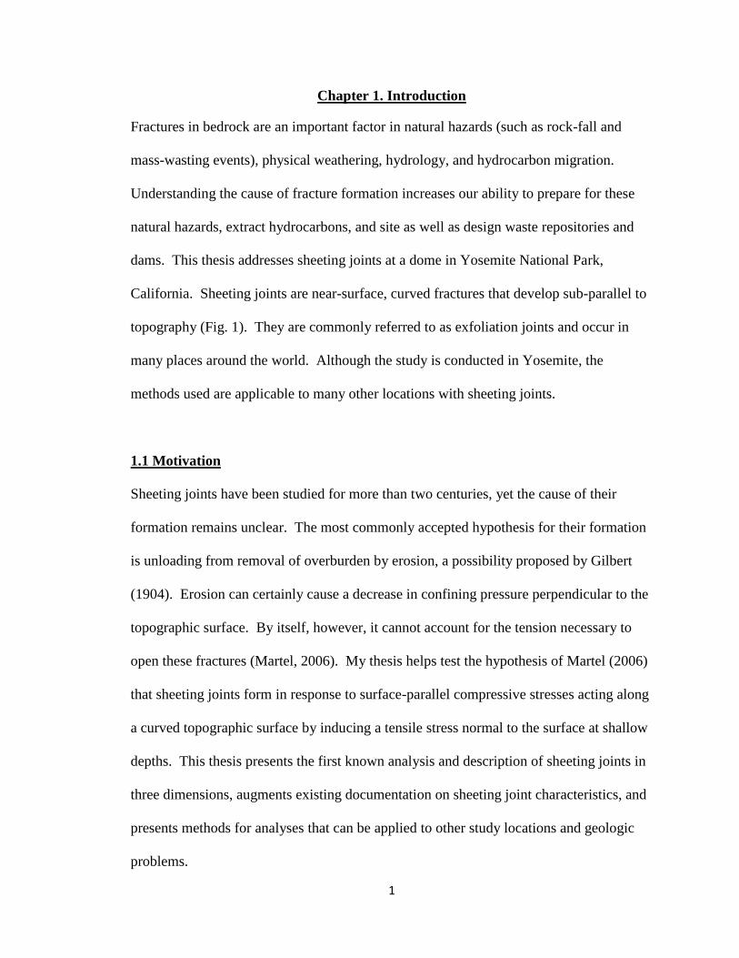
Chapter 1. Introduction
Fractures in bedrock are an important factor in natural hazards (such as rock-fall and
mass-wasting events), physical weathering, hydrology, and hydrocarbon migration.
Understanding the cause of fracture formation increases our ability to prepare for these
natural hazards, extract hydrocarbons, and site as well as design waste repositories and
dams. This thesis addresses sheeting joints at a dome in Yosemite National Park,
California. Sheeting joints are near-surface, curved fractures that develop sub-parallel to
topography (Fig. 1). They are commonly referred to as exfoliation joints and occur in
many places around the world. Although the study is conducted in Yosemite, the
methods used are applicable to many other locations with sheeting joints.
1.1 Motivation
Sheeting joints have been studied for more than two centuries, yet the cause of their
formation remains unclear. The most commonly accepted hypothesis for their formation
is unloading from removal of overburden by erosion, a possibility proposed by Gilbert
(1904). Erosion can certainly cause a decrease in confining pressure perpendicular to the
topographic surface. By itself, however, it cannot account for the tension necessary to
open these fractures (Martel, 2006). My thesis helps test the hypothesis of Martel (2006)
that sheeting joints form in response to surface-parallel compressive stresses acting along
a curved topographic surface by inducing a tensile stress normal to the surface at shallow
depths. This thesis presents the first known analysis and description of sheeting joints in
three dimensions, augments existing documentation on sheeting joint characteristics, and
presents methods for analyses that can be applied to other study locations and geologic
problems.
2
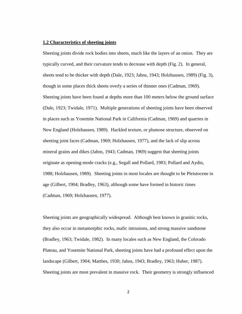
1.2 Characteristics of sheeting joints
Sheeting joints divide rock bodies into sheets, much like the layers of an onion. They are
typically curved, and their curvature tends to decrease with depth (Fig. 2). In general,
sheets tend to be thicker with depth (Dale, 1923; Jahns, 1943; Holzhausen, 1989) (Fig. 3),
though in some places thick sheets overly a series of thinner ones (Cadman, 1969).
Sheeting joints have been found at depths more than 100 meters below the ground surface
(Dale, 1923; Twidale, 1971). Multiple generations of sheeting joints have been observed
in places such as Yosemite National Park in California (Cadman, 1969) and quarries in
New England (Holzhausen, 1989). Hackled texture, or plumose structure, observed on
sheeting joint faces (Cadman, 1969; Holzhausen, 1977), and the lack of slip across
mineral grains and dikes (Jahns, 1943; Cadman, 1969) suggest that sheeting joints
originate as opening-mode cracks (e.g., Segall and Pollard, 1983; Pollard and Aydin,
1988; Holzhausen, 1989). Sheeting joints in most locales are thought to be Pleistocene in
age (Gilbert, 1904; Bradley, 1963), although some have formed in historic times
(Cadman, 1969; Holzhausen, 1977).
Sheeting joints are geographically widespread. Although best known in granitic rocks,
they also occur in metamorphic rocks, mafic intrusions, and strong massive sandstone
(Bradley, 1963; Twidale, 1982). In many locales such as New England, the Colorado
Plateau, and Yosemite National Park, sheeting joints have had a profound effect upon the
landscape (Gilbert, 1904; Matthes, 1930; Jahns, 1943; Bradley, 1963; Huber, 1987).
Sheeting joints are most prevalent in massive rock. Their geometry is strongly influenced
3
by pre-existing structures (Bradley, 1963; Cadman, 1969; Holzhausen, 1989). Sheeting
joints are most commonly observed on convex surfaces, such as domes, but they have
been observed on some concave surfaces such as U-shaped valleys (Gilbert, 1904).
1.3 Previous work
Some of the most notable work on sheeting joints has been done by Gilbert (1904), Dale
(1923), Matthes (1930), Jahns (1943), Bradley (1963), Cadman (1969), and Holzhausen
(1977, 1989). These investigators provide careful descriptions of sheeting joints.
Gilbert (1904) studied the sheeting joints of Yosemite National Park. He observed that:
1) sheeting joints are curved; 2) sheeting joints are present on domes, walls of canyons,
sides of ridges, and locally on valley walls; and 3) glacial polish is observed on sheets
suggesting that sheeting joints pre-date the last glacial episode. Of the three hypotheses
Gilbert considered for sheeting joint formation (surficial thermal effects, weathering, and
unloading from erosion), his "unloading" hypothesis has persisted and has become the
most commonly accepted mechanism (e.g., Chorley, et. al., 1984; Goudie, 2004),
although Gilbert himself did not explicitly endorse this as his favored explanation.
Dale (1923) made several key observations of the commercial granites of New England.
He noted that sheeting joints are sub-parallel to topography, that sheets have a lenticular
shape, and that sheet thickness tends to increase with depth. The most important
observation he made with respect to this thesis is that sheeting joints are present in areas
currently under high surface-parallel compressive stress. The importance of this
4
observation will be explained in detail in chapter 2. Among hypotheses Dale tested and
rejected are that sheeting joints form from insolation, contraction from cooling of the host
intrusive body, tensile stress in the rift direction from cooling, and concentric weathering
due to changes in texture or mineral composition. He could not reject surface-normal
tension, surface-parallel compressive stress, and some combination of insolation near the
surface and surface-parallel compressive stresses at depth as causes. He considered the
last of these hypotheses to be the most plausible cause of sheeting joint formation.
Matthes (1930) studied sheeting joints in his seminal research on Yosemite National
Park. He observed that sheeting joints become less curved and more widely spaced with
depth. The sheets he observed vary in thickness from less than a meter to ~ 30 m.
Matthes recognized that older joints influenced the formation of sheeting joints. He
attributed the sheeting joints to stresses in the rock as opposed to weathering. Matthes
determined that thermal stresses influence sheeting at shallow depths but would not cause
sheeting at depths as great as 30 m. He concluded that Yosemite's famous domes owe
their rounded form to sheeting joints. Finally, Matthes estimated that at least half of the
landscape in Yosemite owed its form to sheeting joints.
Jahns (1943) also studied the granites of New England. He noted that the curvature of
sheeting joints decreases with increased depth; that sheeting joints form independent of
mineral grains, dikes, xenoliths, and country rock; and that sheeting joints are best
developed in sparsely jointed rock masses. An important observation he, like Dale, made
is that New England granites are experiencing high lateral compressive stresses. He

5
postulated several causes for sheeting joint formation, including cooling; local or regional
compressive stress; insolation (daily and secular); hydration and or chemical alteration
(which he rejected); mechanical action of fire, frost, and vegetation; a decrease in
confining pressure by removal of overburden; or some combination of all previously
mentioned causes.
Bradley (1963) worked on sheeting joints of the Colorado Plateau. He observed that
sheeting joints are present there in rocks that were once deeply buried, are of Pleistocene
age, that pre-existing fractures control the prevalence of sheeting joints, and that sheeting
joints are best displayed in thick massive rock units such as sandstones and limestones,
being less prevalent in thinly bedded units. He also noted that sheets exposed during the
construction of Glen Canyon Dam thickened with depth into the canyon wall. He
postulated that sheeting joints form as a result of differential stress from unequal
confining pressure release from erosion.
Cadman (1969) studied sheeting joints of Yosemite National Park in California. He
observed that some sheeting joint surfaces have plumose structure, a feather-like texture
present on opening mode cracks. Cadman made in-situ strain measurements to obtain
stress values at Tuolumne Meadows; these are used in this thesis and will be discussed
further in later chapters. He postulated that sheeting joints result from surface-parallel
compressive stresses.
6
Holzhausen (1977, 1989) studied sheeting joints of New England. He observed that
multiple generations of sheeting joints exist, that younger sheeting joint sheets are
influenced by pre-existing structures, and that the hackle and rib marks like those found
on sheeting joint faces are also found on rock-burst faces in quarries suggesting that
sheeting joints grow rapidly. Holzhausen (1977) tested the hypothesis of Dale, that
sheeting joints form in response to high compressive stresses parallel to the ground
surface, and he could not reject it. He concluded that sheeting joints form from high
differential stress, dominated by high compressive stresses parallel to an exposed rock
surface. He also suggested that the cause of this high differential stress could be from
vertical unloading by erosion.
A recurring theme is that sheeting joints are most prominent on domes experiencing
surface-parallel compressive stresses (Martel, 2006). Holzhausen (1977) and Miller and
Dunne (1996) have suggested on theoretical grounds that sheeting joints are related to
strong compressive stresses parallel to topography, but they did not test the idea with real
topographic data.
Martel (2006) derived a two-dimensional expression of equilibrium to explain the
formation of sheeting joints. The key factors are surface-parallel stress, surface
curvature, and body forces. He tested his hypothesis using topographic data and stress
values from 9 locales across the U. S. and concluded that the sheeting joints present at 7
of the 9 locales can be accounted for by a combination of highly compressive surface-
parallel stresses and topographic curvature.
7
1.4 Hypothesis to be tested
My research further tests Martel‟s (2006) hypothesis that sheeting joints form in response
to surface-parallel stresses acting along a curved topographic surface. This thesis will
address two items that were not previously adequately addressed together: 1) a three-
dimensional shape of sheeting joints and topography (based on surface curvature), and 2)
three-dimensional mechanical analyses for sheeting joint formation. The main focus is
on whether sheeting joints at a particular dome in Yosemite National Park, referred to
here as Tenaya Creek (TC) Dome, and the surrounding area be accounted for by modern
topography and stresses.
1.5 Study area
Yosemite National Park, located in east-central California (Fig. 4), is well known for its
vast expanses of granites and spectacular displays of sheeting joints (e.g., Matthes, 1930).
It was selected for study because of its high quality sheeting joint exposures. The Tenaya
Lake region extends over 77 km2 near the center of the park (Figs. 4 and 5). Perhaps the
single most striking display of sheeting joints in the Tenaya Lake region occurs at TC
Dome along the northwest margin of Tenaya Canyon (Figs. 5 and 6). TC Dome is
located at UTM 282491 northing, 4187365 easting, zone 11 (Fig. 6); its summit
elevation is 2491 m. TC Dome has a gross doubly-convex shape (this will be discussed
further subsequently). It is bordered by a ridge to the north-northeast, Tenaya Canyon to
the east-southeast, and immediately to the east by Tenaya Creek (Fig. 6). This thesis
8
focuses on the TC Dome study area, but also utilizes observations from elsewhere in the
Tenaya Lake region.
1.6 Outline
The remainder of this thesis presents field observations coupled with topographic and
mechanical analyses to determine whether or not sheeting joints at TC Dome may be
accounted for by the modern stress state and current topography. Two key factors in the
analyses are surface-parallel stresses and surface curvature. The mechanical hypothesis
being tested is explained in detail in chapter 2. Chapter 3 presents a tutorial of surface
curvature, a concept from differential geometry that has only recently begun to be used in
geology (e.g., Bergbauer, 2002; Pearce et. al, 2006). Chapter 4 presents geologic
observations from the Tenaya Lake region and TC Dome, and describes the relative ages
of structural features at TC Dome and East Ridge (Fig. 6). Chapter 5 discusses the
collection, processing, and quality of aerial LIDAR data for the Tenaya Lake region. In
chapter 6, stress and topographic analyses are presented for the TC Dome study area.
Finally, chapter 7 discusses the findings and presents the key conclusions.
9
Chapter 2. Mechanical Hypothesis
Observations of sheeting joint faces overwhelmingly favor an opening-mode formation.
Opening-mode, or mode I, fractures can open in one of two ways. Either a far-field stress
normal to the fracture must be tensile, or the internal pressure (such as a fluid pressure)
acting within the fracture must exceed the far-field compressive stress acting to close it
(e.g., Pollard and Segall, 1987). One would anticipate either chemical alteration on
sheeting joint faces or mineralization within the joints if they were opened by fluid
pressure. Other than iron oxide stains along some sheeting joints, neither chemical
alteration nor mineralization was observed along sheeting joints at TC Dome. Therefore,
tension is required in order to open these joints.
The commonly accepted hypothesis that sheeting joints form in response to removal of
overburden is not mechanically acceptable because removal of overburden, by itself,
merely decreases the compressive stress normal to the topographic surface. While this
reduction of vertical compressive stress will lead to a positive elastic strain (extension)
normal to the surface, this does not equate to a tensile stress necessary to open a sheeting
joint. In contrast, tension perpendicular to sheeting joint walls can be induced by high
compressive stresses acting parallel to a convex topographic surface (Martel, 2006).
Figure 7 illustrates in two dimensions how a compressive stress (P) acting parallel to an
infinitesimal convex surface element along the ground surface can induce a tension
normal to the surface (N). Throughout the thesis, tension is considered as positive (hence
compression is negative). Curvature is positive if concave (and negative if convex). The
10
convex upper surface of the element in Fig. 7 is traction free, and no shear tractions (τ)
exist on the boundaries of the element. The compressive (negative) tractions on the
element ends induce a force directed away from the center of curvature (Fr) that must be
opposed by tensile tractions (N) perpendicular to the base of the element in order to
maintain equilibrium (Martel, 2006).
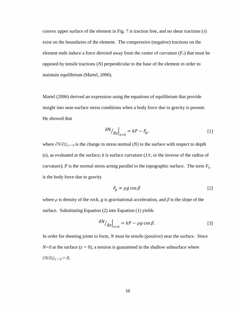
Martel (2006) derived an expression using the equations of equilibrium that provide
insight into near-surface stress conditions when a body force due to gravity is present.
He showed that
, [1]
where ∂N/∂z|z = 0 is the change in stress normal (N) to the surface with respect to depth
(z), as evaluated at the surface; k is surface curvature (1/r, or the inverse of the radius of
curvature); P is the normal stress acting parallel to the topographic surface. The term Fg
is the body force due to gravity
[2]
where ρ is density of the rock, g is gravitational acceleration, and β is the slope of the
surface. Substituting Equation (2) into Equation (1) yields
. [3]
In order for sheeting joints to form, N must be tensile (positive) near the surface. Since
N=0 at the surface (z = 0), a tension is guaranteed in the shallow subsurface where
∂N/∂z|z = 0 > 0.
11
Equation (3) pertains strictly to a profile across cylindrical topography, but it may be
expanded to a three-dimensional solution for use with topographic surfaces of arbitrary
shape (Martel, 2005):
[4]
where k1 and k2 are principal curvatures, P1 and P2 are normal stresses acting along the
directions of the principal curvatures, and β is the slope. Surface curvature will be
described in detail in the following chapter. For now, it suffices to say that the shape of a
topographic surface at a point can be described by the maximum and minimum
curvatures k1 and k2. Equation (4) allows one to predict conditions under which sheeting
joints could or should not nucleate based on topographic geometry and surface-parallel
stresses.
Threshold conditions for sheeting joint formation are set by the ρgcosβ term of Equation
(4). Assuming that sheeting joints open in tension, a necessary condition for sheeting
joint nucleation would be that k1P1+k2P2 ≥ ρgcosβ. In other words, the stress gradient
acting to open the fracture (k1P1+k2P2) exceeds that acting to close the fracture (ρgcosβ).
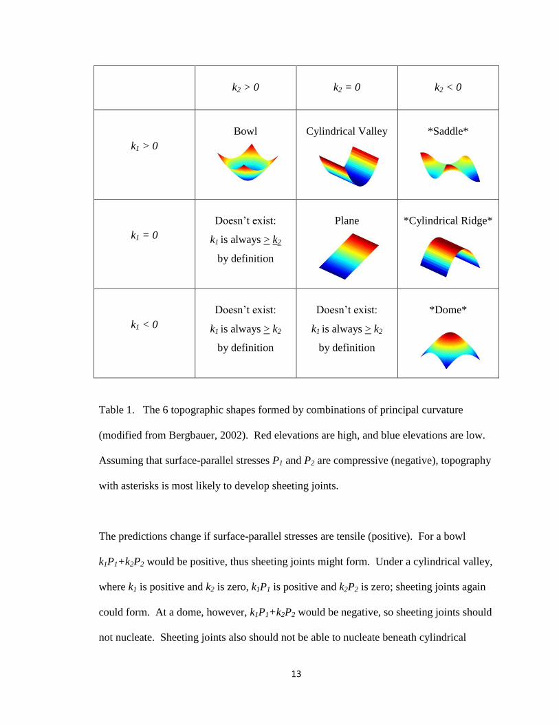
Table 1 illustrates topographic shapes based upon combinations of principal curvatures.
Those model landforms shown with an asterisk are most susceptible to developing
sheeting joints if surface-parallel stresses P1 and P2 are compressive (negative) and of
large magnitude, as is the case in the Tenaya Lake region (Cadman, 1969). For a dome,
both principal curvatures are negative, so k1P1+k2P2 would be positive, and sheeting
joints could develop if that sum exceeds ρgcosβ. Sheeting joints could develop in a
12
cylindrical ridge because even though k1 equals 0, k2 is negative, so k1P1+k2P2 could still
be positive and exceed ρgcosβ. For a bowl, however, both k1 and k2 are positive, hence
k1P1+k2P2 would be negative. According to the conditions of Equation (4), sheeting
joints should not nucleate beneath a bowl. Sheeting joints should not nucleate beneath a
cylindrical valley either because k1 is positive and k2 is zero, hence k1P1+k2P2 would be
negative. For a perfect plane (which is unlikely to exist in nature) both principal
curvatures equal zero, so sheeting joints should not nucleate beneath a perfectly planar
surface. For a saddle, perhaps the most common topographic shape, k1 and k2 have
opposite signs. Whether or not sheeting joints develop beneath a saddle depends on the
relative and absolute magnitudes of the products k1P1 and k2P2. Where k2P2 (the “convex
contribution”) sufficiently exceeds k1P1 (the “concave contribution”), sheeting joints
could form. Thus, assuming surface-parallel stresses are compressive, sheeting joints are
most likely to nucleate at domes, cylindrical ridges, and some saddles, but not at bowls,
cylindrical valleys, and perfect planes.
13
k2 > 0
k2 = 0
k2 < 0
k1 > 0
Bowl
Cylindrical Valley
*Saddle*
k1 = 0
Doesn‟t exist:
k1 is always > k2
by definition
Plane
*Cylindrical Ridge*
k1 < 0
Doesn‟t exist:
k1 is always > k2
by definition
Doesn‟t exist:
k1 is always > k2
by definition
*Dome*
Table 1. The 6 topographic shapes formed by combinations of principal curvature
(modified from Bergbauer, 2002). Red elevations are high, and blue elevations are low.
Assuming that surface-parallel stresses P1 and P2 are compressive (negative), topography
with asterisks is most likely to develop sheeting joints.
The predictions change if surface-parallel stresses are tensile (positive). For a bowl
k1P1+k2P2 would be positive, thus sheeting joints might form. Under a cylindrical valley,
where k1 is positive and k2 is zero, k1P1 is positive and k2P2 is zero; sheeting joints again
could form. At a dome, however, k1P1+k2P2 would be negative, so sheeting joints should
not nucleate. Sheeting joints also should not be able to nucleate beneath cylindrical
14
ridges if surface-parallel stresses are tensile because k1 is zero and k2 is negative, so k1P1
would be zero and k2P2 would be negative. Because perfect planes have principal
curvatures of zero, sheeting joints should not nucleate regardless of whether surface-
parallel stresses are compressive or tensile. Sheeting joints could still form beneath a
saddle if k1P1 (the “concave contribution”) sufficiently exceeds the absolute magnitude of
k2P2 (the “convex contribution”). Thus, assuming surface-parallel stresses are tensile
sheeting joints are most likely to nucleate at bowls, cylindrical valleys, and some saddles,
but not at domes, cylindrical ridges, and perfect planes. Sheeting joints are less likely to
form where surface-parallel stresses are tensile rather than compressive, however. This is
because rocks are relatively weak in tension and hence are unlikely to be able to sustain
surface-parallel tensile stresses large enough for the sum of the kP products to be large
enough to promote the opening of sheeting joints.
In summary, according to Equation (4), sheeting joint nucleation depends upon surface
curvature, surface-parallel stresses, the unit weight of the rock (ρg) and the slope. The
shape of the topographic surface can act to either permit or preclude the formation of
sheeting joints. Sheeting joints should not nucleate beneath a broad perfectly planar
surface, regardless of the sign of surface-parallel stresses. Beneath saddles, sheeting
joints could nucleate regardless of the sign of surface-parallel stresses. In regions where
surface-parallel stresses are tensile everywhere, sheeting joints could nucleate under
bowls, cylindrical valleys, and saddles; they are unlikely to nucleate beneath planes,
cylindrical ridges, and domes. Where surface-parallel stresses are compressive (such as
in the Tenaya Lake region), sheeting joint nucleation is most likely beneath domes,
15
cylindrical ridges, and saddles, and least likely beneath perfect planes, bowls, and
cylindrical valleys. This thesis uses the 3d expression of equilibrium (Eqn. 4) derived by
Martel (2006) to test whether or not the current topography and the stresses parallel to the
topographic surface at TC Dome can account for the formation of geologically young
sheeting joints.
16
Chapter 3. Curvature Tutorial
This chapter presents a brief tutorial of curvature for plane curves (two-dimensional) and
surfaces (three dimensional), both of which were used for topographic analyses
throughout this research. Curvature formulas are not derived here but can be found
elsewhere (e.g., Struik, 1961; Bergbauer and Pollard, 2003; Mynatt et. al, 2007).
Common usage to the contrary, the curvature of a plane curve is not merely the second
derivative, and the curvature of a surface is not merely the Laplacian. The second
derivative and Laplacian provide good estimates of curvature only in special cases.
3.1 Curvature of a plane curve
The curvature at a point along a plane curve is defined as the rate of change of a unit
tangent, or unit normal, with respect to distance along a curve (e.g., Bergbauer, 2002).
The curvature at a point along a plane curve y = y(x) is (e.g., Leithold, 1976; Roberts,
2001)
,
[5]
where y' and y" are the first and second derivatives of y with respect to x. The second
derivative equals the curvature only where the first derivative equals zero (i.e., at a local
maximum or minimum along a plane curve).
Perhaps the simplest plane curve is a circular arc (Fig. 8). Using three points, the radius
(r) of a circular arc can be obtained by fitting a circle to the three points, with the center
being at the intersection of perpendicular bisectors between line segments connecting
pairs of points. The curvature for a circular arc is the inverse of its radius. Another way
17
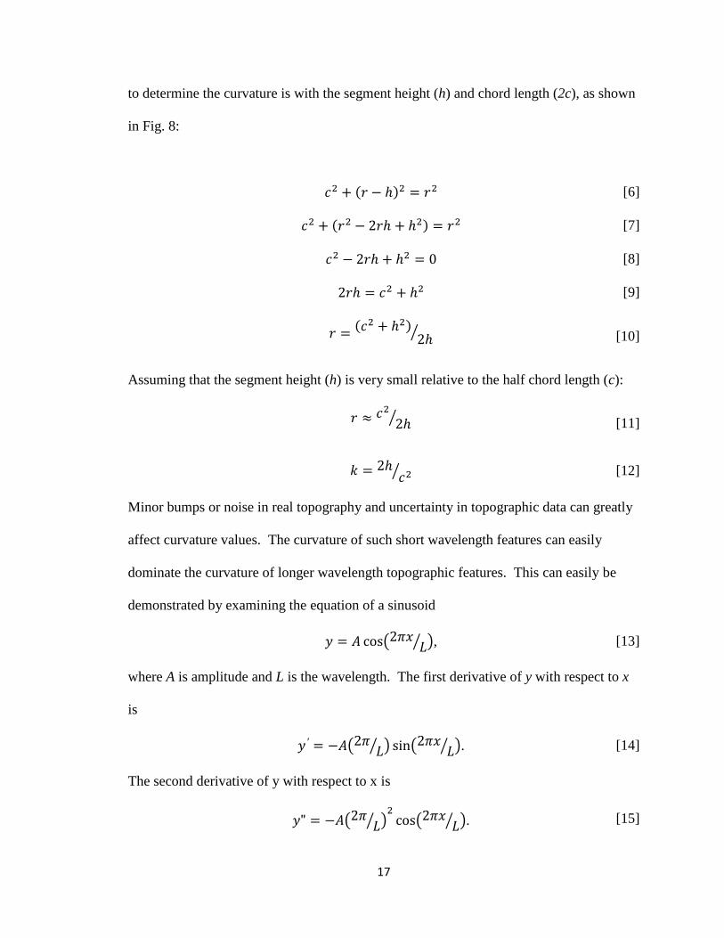
to determine the curvature is with the segment height (h) and chord length (2c), as shown
in Fig. 8:
[6]
[7]
[8]
[9]
[10]
Assuming that the segment height (h) is very small relative to the half chord length (c):
[11]
[12]
Minor bumps or noise in real topography and uncertainty in topographic data can greatly
affect curvature values. The curvature of such short wavelength features can easily
dominate the curvature of longer wavelength topographic features. This can easily be
demonstrated by examining the equation of a sinusoid
, [13]
where A is amplitude and L is the wavelength. The first derivative of y with respect to x
is
. [14]
The second derivative of y with respect to x is
. [15]
18
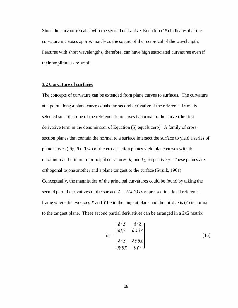
Since the curvature scales with the second derivative, Equation (15) indicates that the
curvature increases approximately as the square of the reciprocal of the wavelength.
Features with short wavelengths, therefore, can have high associated curvatures even if
their amplitudes are small.
3.2 Curvature of surfaces
The concepts of curvature can be extended from plane curves to surfaces. The curvature
at a point along a plane curve equals the second derivative if the reference frame is
selected such that one of the reference frame axes is normal to the curve (the first
derivative term in the denominator of Equation (5) equals zero). A family of cross-
section planes that contain the normal to a surface intersect the surface to yield a series of
plane curves (Fig. 9). Two of the cross section planes yield plane curves with the
maximum and minimum principal curvatures, k1 and k2, respectively. These planes are
orthogonal to one another and a plane tangent to the surface (Struik, 1961).
Conceptually, the magnitudes of the principal curvatures could be found by taking the
second partial derivatives of the surface Z = Z(X,Y) as expressed in a local reference
frame where the two axes X and Y lie in the tangent plane and the third axis (Z) is normal
to the tangent plane. These second partial derivatives can be arranged in a 2x2 matrix
[16]

19
This real matrix is symmetric (the entry in the upper right matches the entry in the lower
left), and hence can be re-expressed in the following form if the X-axis is aligned with
the k1-direction (Strang, 1998):
[17]
Calculation of the magnitudes and directions of the principal curvatures is not trivial in
practice, however, and the interested reader should consult references for details (e.g.,
Struik, 1961; Bergbauer and Pollard, 2003; Pollard and Fletcher, 2005).
Two principal curvatures completely describe the shape of a surface at a point.
Analogous to curvature for plane curves, the principal curvatures for a point on a surface
involve combinations of first and second partial derivatives of elevation (z) with respect
to easting (x) and northing (y); see Struik (1961) and Bergbauer and Pollard (2003) for
details. The principal curvatures are orthogonal, with one direction marking the most
positive curvature and the other the most negative curvature (e.g., Struik, 1961).
Although principal curvature directions at a point are orthogonal in a tangent plane, their
trends in map view are usually not. In the previous chapter, various combinations of k1
and k2 were used to illustrate topographic shapes (Table 1). Two other parameters based
on principal curvatures are frequently used to describe topographic shapes as well: mean
curvature (H) and Gaussian curvature (K). The mean curvature (H) is the mean value of
k1 and k2. Gaussian curvature is the product of k1 and k2. Table 2 illustrates topographic
shapes based upon combinations of mean and Gaussian curvature.
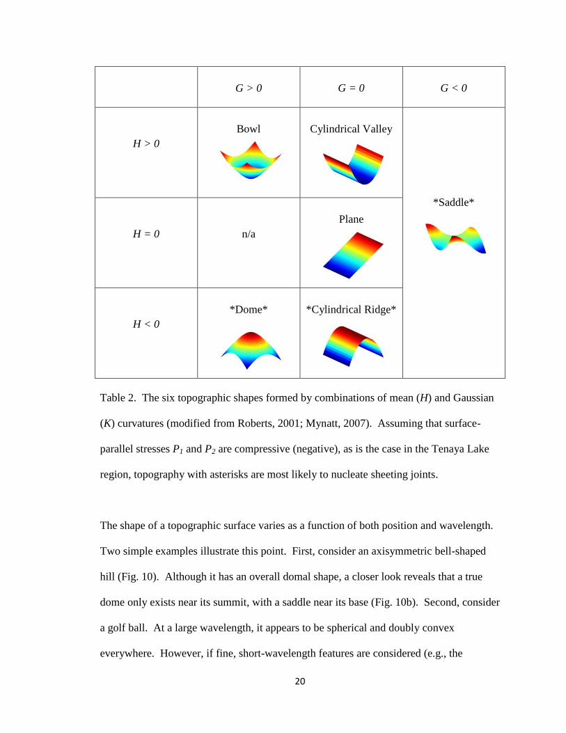
20
G > 0
G = 0
G < 0
H > 0
Bowl
Cylindrical Valley
*Saddle*
H = 0
n/a
Plane
H < 0
*Dome*
*Cylindrical Ridge*
Table 2. The six topographic shapes formed by combinations of mean (H) and Gaussian
(K) curvatures (modified from Roberts, 2001; Mynatt, 2007). Assuming that surface-
parallel stresses P1 and P2 are compressive (negative), as is the case in the Tenaya Lake
region, topography with asterisks are most likely to nucleate sheeting joints.
The shape of a topographic surface varies as a function of both position and wavelength.
Two simple examples illustrate this point. First, consider an axisymmetric bell-shaped
hill (Fig. 10). Although it has an overall domal shape, a closer look reveals that a true
dome only exists near its summit, with a saddle near its base (Fig. 10b). Second, consider
a golf ball. At a large wavelength, it appears to be spherical and doubly convex
everywhere. However, if fine, short-wavelength features are considered (e.g., the

21
dimples on the ball), then much of the surface would be seen to be doubly concave
(bowl-shaped). Sample spacing and wavelength thus play key roles in the determination
of curvature.
22
Chapter 4. Geology
Yosemite National Park, located in east-central California (Fig. 4), is well known for its
vast expanses of granitic rock and spectacular displays of sheeting joints (e.g., Matthes
1930). It was selected for study because of its quality of sheeting joint exposures. Aerial
LIDAR (Light Detection and Ranging) data were collected by NCALM (National Center
for Airborne Laser Mapping) over 77 km2 of the Tenaya Lake region (Fig. 5) of
Yosemite stretching approximately from Tuolumne Meadows to Olmsted Point, in the
late summer of 2006. The LIDAR data were collected for topographic analyses, and in
the hope that sheeting joints could be mapped from these data as well. Details of the
LIDAR data collection and its collection are presented in chapter 5.
4.1 Geologic overview of the Tenaya Lake region
Two igneous bodies from the Tuolumne Meadows Intrusive Suite underlie the Tenaya
Lake study area: the Cathedral Peak Granodiorite and the Half Dome Granodiorite (e.g.,
Huber, 1987). The Tuolumne Intrusive Suite was assembled over a period of roughly 10
m.y. between 95 Ma and 85 Ma, based on U-Pb dating (Glazner, et al., 2004). The Half
Dome Granodiorite was assembled over a period of nearly 4 m.y. from ~88 Ma to ~91
Ma (Coleman et al., 2004). The Half Dome Granodiorite is medium-grained, light-gray
in color, and composed of plagioclase, quartz, orthoclase, biotite, and hornblende
(Matthes, 1930). The Cathedral Peak Granodiorite was emplaced ~88 Ma. The
Cathedral Peak Granodiorite is easily recognized by its large (~10-20 cm) potassium
feldspar phenocrysts; its groundmass is composed of small grains of quartz, feldspar, and
23
minor amounts of biotite and hornblende (Matthes, 1930). TC Dome is composed of
Half Dome Granodiorite.
The uplift of the Sierra Nevada Range is a matter of renewed debate (e.g., Henry, 2009).
Some workers suggest that the Sierra Nevada was uplifted during the late Cenozoic ~10
Ma (Unruh, 1991; Wakabayashi and Sawyer, 2001), mainly through a westward tilting of
the range. In contrast, others argue that the range was uplifted in the late Mesozoic and
remained high in the Cenozoic (Small and Anderson, 1995; Wernicke et al., 1996). They
postulate that subsidence of the Basin and Range is responsible for faulting on the eastern
flank of the Sierra Nevada, as opposed to uplift of the Sierra. Based on isotopic
evidence, Cassel et al. (2009) concluded that the paleo-elevation of the northern
Sierra Nevada 31-28 Ma was similar to what is observed today, providing support that
most uplift occurred in the Late Cretaceous to early Cenozoic. Much of the current local
topography in the High Sierra, which includes Yosemite National Park, is nonetheless
likely to be of Quaternary age owing to extensive glaciation (e.g., Bateman and
Wahrhaftig, 1966; Gillespie, 1982; Phillips et al., 1996).
4.2 Sheeting joints of the Tenaya Lake region
Sheeting joints are prominently exposed throughout much of the Tenaya Lake region.
Some of the most notable locations include Clouds Rest, Cathedral Peak, Tenaya Peak, a
dome located immediately southwest of Tenaya Lake (282290 northing, 4188130 easting,
with a summit elevation of ~2586 m), Matthes Crest, Olmsted Point, a bowl (281355
northing, 4188295 easting) ~500m north of Olmsted Point, Tioga Road quarry and the
24
ridge containing it (278943 northing, 4187788 easting) ~3 km west of Olmsted Point,
May Lake, and numerous other areas along Tioga Road (Fig. 5).
In many locales where sheeting joints are not immediately apparent they can be observed
upon closer examination. Pothole Dome and the dome near BM 8452 (285854 northing,
4193386 easting), both in the northeastern part of the study area, appear to have few
sheeting joints. Pothole Dome has extensive glacial polish, potholes, and glacial flutes.
Sheeting joints crop out locally, but might have been more widespread and plucked away
by Pleistocene glaciers. Near the top of Pothole Dome, sheeting joints decorate the west
side of a natural amphitheater (Fig. 11a). Many of these joints do not parallel the modern
topography, indicating substantial erosion since the joints formed. At the dome near
benchmark 8452, across Tioga Road from Medlicott Dome, the southeastern face appears
nearly devoid of sheeting joints, but the northwestern face has heavily weathered sheeting
joint steps (Fig. 11b). Most of the southeastern face displays glacial polish and, upon
close examination, sheeting joint traces are observed there as well.
4.2.1 Characteristics
Sheeting joints and sheets in the Tenaya Lake region have many common characteristics.
Generally, sheets thicken with depth (e.g., Fig. 3), consistent with the findings of Jahns
(1943) for New England. This is not the case everywhere, though. Some sheets near the
base of TC Dome and at road-cuts along Tioga Road thin with depth. In some places
multiple generations of sheeting joints exist. At Mount Hoffman, two sets of sheeting
joints are present on an arête; the older set parallels an ancient topographic surface prior
25
to the last glacial erosion and the younger mimics modern topography (USGS, n.d.).
Sheets tend to have a lenticular shape. In many locations, water stains develop down-
slope of where sheeting joints daylight, and in several locales water was observed
flowing out of sheeting joints (Fig. 12). Sheeting joints and other fractures are a
particularly important factor in the shallow hydrology of the Yosemite region because the
host crystalline rock has virtually no intrinsic interconnected pore structure.
Sheeting joints of the Tenaya Lake region, like those studied elsewhere by other
researchers, exhibit evidence that they originate as opening mode (mode I) fractures
(Holman, 1976; Holzhausen, 1989; Bahat et. al, 1999) rather than as shear (mode II or
III) fractures. Hackled sheeting joint faces exist in several locales, for example on the
southwest face of Pywiak Dome along Tioga Road, and on the northwest face of the ridge
containing the Tioga Road quarry (Fig. 13). Where sheeting joints cut dikes, xenoliths,
and phenocrysts, no offset is visible (Figs. 11 and 14). All of these observations indicate
that sheeting joints in Tenaya Lake region formed as opening-mode fractures. If sheeting
joints opened in response to elevated fluid pressures in the rock, then hydro-chemical
alteration or mineralization might be expected along the joints. Fresh sheeting joint faces
in this region, however, generally are not chemically altered. These observations support
the idea that sheeting joints open in tension, not in response to elevated fluid pressure.
4.2.2 Age
Most sheeting joints mimic modern topography, and therefore are unlikely to be older
than the Pleistocene. Glacial polish burnishes many sheeting joint faces, demonstrating
26
that at least some sheeting joints were formed and uncovered prior to the retreat of Tioga-
age glaciers approximately 13,000 years ago (Clark, 1995). Other sheeting joints have
formed within the last few decades. Cadman (1969) deduced that sheeting joints near
Olmsted Point have formed since blasting occurred for the construction of Tioga road,
which occurred between 1957 and 1961 (Trexler, 1961). Furthermore, some sheeting
joints terminate against boreholes drilled in the quarry during the construction of Tioga
road, suggesting that sheeting joints may still be forming.
4.3 Geologic structures of the TC Dome study area
TC Dome, located where the hanging valley of Tenaya Creek drops into Tenaya Canyon
(Figs. 5 and 6), displays a spectacular array of sheeting joints (Figs. 14-19). The UTM
coordinates of the summit of TC Dome are approximately 282491 northing and 4187365
easting, with a summit elevation of 2491 m. Tenaya Creek flows southeast between TC
Dome and a ridge to the northeast (the "East Ridge"). Both TC Dome and the East Ridge
display (1) an impressive array of sheeting joints (Fig. 15-18), and (2) large planar
fractures that define domains of sheeting joints (Figs. 15, 17, and 18). In addition to
these prominent features, dikes, glacial polish, and relatively small fractures (< 2 m long)
occur.
The distribution, kinematics, and geometry of sheeting joints at TC Dome study area
were documented with photographs (e.g., Figs. 14-19), attitude measurements on
individual sheeting joint faces (appendix A), and a fracture map (Fig. 20). The fracture
map was made from more than 2,200 points surveyed using a Topcon 206, 0°0'06" total
27
station instrument. The total station occupied one base station location (282543.6
easting, 4187403.8 northing, and 2451.0 m elev.) and a back-sight was set across Tenaya
Canyon (282754.4 easting, 4187266.9 northing, and 2432.6 m elev.). The GPS
coordinates were recorded at the base station and back-sight locations using a Geneq
(SXBlue) GPS unit with < 2.5 m accuracy. Figures 15-19 show dikes in red and other
fractures in blue. Circled numbers mark prominent features: domains of sheeting joints
(numbers 1 and 2) and a scarp (number 3); see Fig. 16. The approximate extent of
mapping in Fig. 20 is shown in bright green in Figs. 16 and 17.
4.3.1 Structural features older than the sheeting joints
Two aplite dikes (D1 and D2 shown in red on Figs. 16-18, and 20) extend across Tenaya
Creek at TC Dome study area. They trend north-northeast, roughly parallel to Tenaya
Canyon. D1 strikes N67°W, dipping 21°NE and D2 strikes N63°W, dipping 34°NE.
Their lengths exceed 60 meters and they are approximately 0.3 meters thick. Because D1
and D2 extend across both TC Dome and East Ridge and do not cut any fractures, they
are likely to be the oldest geologic structures of the study area.
Group F includes fractures F1-F10 (Fig. 20). They are present on either side of Tenaya
Creek, but none cross either the streambed or the steeply dipping fracture (F1) along the
streambed. Group F fractures are at least several meters long, with apertures of less than
5 cm. Fractures F2 and F4 exceed 40 meters in length. The fractures appear to lack
mineral fillings. No lateral slip was observed across fracture faces where they cut dikes,
28
but the geometry of both the dikes and F fractures are such that slip would not be easily
detectable. Orientation data for fractures F1-F10 are shown in Table 3 and Fig. 21.
Group F fractures are younger than dikes D1 and D2 because they cut the dikes. The
relative ages of the F-fractures cannot be determined with certainty. Fracture F6
terminates against F4, suggesting that F4 is the older of the two fractures. Sheeting joints
terminate against F fractures but do not cross them, suggesting that F-fractures are older
than sheeting joints at TC Dome study area.
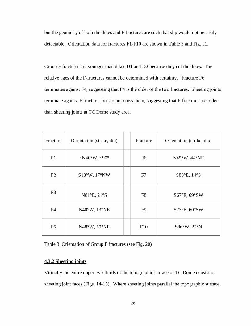
Fracture
Orientation (strike, dip) Fracture Orientation (strike, dip)
F1
~N40°W, ~90° F6 N45°W, 44°NE
F2
S13°W, 17°NW F7 S88°E, 14°S
F3
N81°E, 21°S
F8
S67°E, 69°SW
F4
N40°W, 13°NE F9 S73°E, 60°SW
F5
N48°W, 50°NE F10 S86°W, 22°N
Table 3. Orientation of Group F fractures (see Fig. 20)
4.3.2 Sheeting joints
Virtually the entire upper two-thirds of the topographic surface of TC Dome consist of
sheeting joint faces (Figs. 14-15). Where sheeting joints parallel the topographic surface,
29
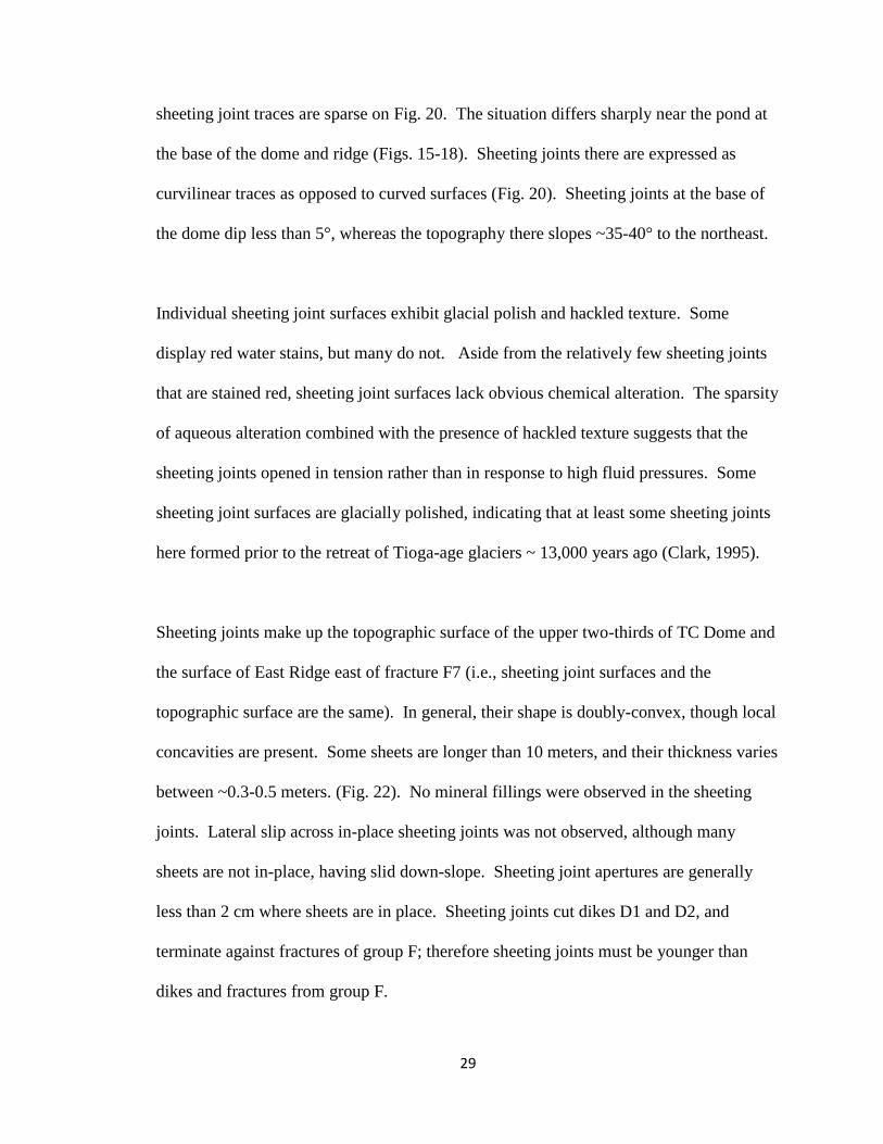
sheeting joint traces are sparse on Fig. 20. The situation differs sharply near the pond at
the base of the dome and ridge (Figs. 15-18). Sheeting joints there are expressed as
curvilinear traces as opposed to curved surfaces (Fig. 20). Sheeting joints at the base of
the dome dip less than 5°, whereas the topography there slopes ~35-40° to the northeast.
Individual sheeting joint surfaces exhibit glacial polish and hackled texture. Some
display red water stains, but many do not. Aside from the relatively few sheeting joints
that are stained red, sheeting joint surfaces lack obvious chemical alteration. The sparsity
of aqueous alteration combined with the presence of hackled texture suggests that the
sheeting joints opened in tension rather than in response to high fluid pressures. Some
sheeting joint surfaces are glacially polished, indicating that at least some sheeting joints
here formed prior to the retreat of Tioga-age glaciers ~ 13,000 years ago (Clark, 1995).
Sheeting joints make up the topographic surface of the upper two-thirds of TC Dome and
the surface of East Ridge east of fracture F7 (i.e., sheeting joint surfaces and the
topographic surface are the same). In general, their shape is doubly-convex, though local
concavities are present. Some sheets are longer than 10 meters, and their thickness varies
between ~0.3-0.5 meters. (Fig. 22). No mineral fillings were observed in the sheeting
joints. Lateral slip across in-place sheeting joints was not observed, although many
sheets are not in-place, having slid down-slope. Sheeting joint apertures are generally
less than 2 cm where sheets are in place. Sheeting joints cut dikes D1 and D2, and
terminate against fractures of group F; therefore sheeting joints must be younger than
dikes and fractures from group F.
30
Sheeting joints near the pond, on both TC Dome and East Ridge, are not parallel to the
topographic surface. The topographic surface slopes ~40-50° to the northeast at the base
of TC Dome, and ~30° to the southwest at East Ridge. Sheeting joint traces near the
pond trend north-northwest, sub-parallel to Tenaya Creek. On TC Dome, sheeting joints
near the pond are divided into two domains based upon their geometry and location
relative to fracture F2. Sheeting joints beneath or east of F2, and north of F3 are in
domain 1. Domain 1 sheeting joints dip less than 5° and are closely spaced (< 0.2 m)
(Fig. 22). Domain 2 sheeting joints, west of F2, are spaced less than 0.5 meters apart,
and curve sharply toward fracture F2. The dihedral angle between F2 and the sheeting
joints is approximately 45-60°. Sheeting joints on East Ridge near the pond dip 10-20° to
the southwest and are spaced less than 0.5 meters apart. Their apertures are less than 2
cm. No lateral slip was observed across sheeting joints near the pond. Sheeting joints
near the pond cut dikes D1 and D2 and terminate against fractures of group F, so sheeting
joints near the pond must be the youngest of these features.
4.3.3 Structural features younger than the sheeting joints
Group O fractures strike north-northeast, dip steeply (~ 80-90°), and are relatively short,
with lengths ranging from 0-3 meters. As with the other planar fracture groups,
O-fractures show no mineral fill and are not water stained. Group O fractures terminate
against F-fractures, indicating that O fractures are younger than F-fractures and hence
younger than the dikes too. Some sheeting joints terminate against fractures from group
31
O, however, at least one O-fracture terminates against sheeting joints, so the relative ages
of O-fractures and sheeting joints are unclear.
At least one sheet on TC Dome is fractured and buckled (B1 on Figs. 18 and 19).
Fracture B1 strikes N45°E along the hinge of the buckle and dips ~ 90. No lateral slip
was observed across B1, and aperture is ~ 1 cm. The presence of a buckled sheet
suggests that, at least recently, the area has been influenced by high surface-parallel
compression (Ericson and Olvmo, 2004).
32
Chapter 5. Aerial LIDAR Data
Aerial LIDAR data, along with aerial photographs, were collected by NCALM over the
Tenaya Lake region. The objective was to use these data for topographic analyses, and
mapping of individual sheeting joints. An overview of NCALM's data collection and
pre-processing is presented below; additional details can be found in NCALM's
processing report.
5.1 Data collection
Aerial LIDAR data were collected by NCALM on September 18 and September 22,
2006. Spatial data were collected with an Optech 1233 ALTM (serial #99B112) mounted
in a turbocharged twin engine Cessna 337 (tail number N86539). Color images were
acquired using a Redlake MS 4100 digital camera; however, the photographs were
overexposed and are not used in this thesis. Flight line spacing was held constant at 200
m. Because the flight line spacing was held constant and the height above terrain varied,
overlap percentages between swaths vary. The scan angle was held constant at ±19°, and
scan frequency (mirror oscillation frequency) was fixed at 30 Hz.
For the Tenaya Lake region, flying heights averaged approximately 1,000 m above the
ground surface. At this height, the cross-track point spacing is 1.2 m. The along-track
point spacing depends on the ground speed of the aircraft which averaged approximately
125 knots. The along-track spacing is approximately 1.1 m at nadir and increases up to
2.2 m at the swath edge. Swath width is 670 m and laser spot size is 0.30 m. Project

33
flight lines were oriented east-northeast, with cross-lines being flown perpendicular to
project flight lines.
GPS reference stations were set up at Olmsted Point and Pothole Dome. All observations
were submitted to the NGS on-line processor OPUS with solution files included in
Appendix A of NCALM‟s processing report. Final NAD83 UTM coordinates were
obtained from the OPUS solutions. Estimated horizontal errors are less than 8 cm, with
vertical errors less than 10 cm.
5.2 Calibration and point cloud data
The relative calibration procedure NCALM uses has cross-lines flown for every flight
with a heading perpendicular to the project flight line heading. Small polygons
containing both the cross lines and project flight lines are processed using approximate
calibration values for heading, roll, pitch, and scanner mirror scale. All lines are
processed separately and then filtered to remove vegetation. Individual flight line
surfaces are then created. An iterative algorithm then computes the best fit between
overlapping flight line surfaces, simultaneously accounting for heading, roll, pitch, and
scanner mirror scale. The output is checked for all flights using each flight‟s cross lines.
Each flight is calibrated by comparing the height of the nearest neighbor laser point to the
height of a set of check points collected by vehicle-mounted GPS.
The data received from NCALM include a 9 column ASCII file (space delimited), with
one file per flight strip. The columns are: GPS time (seconds of week), easting last
34
return, northing last return, height last return, intensity last return, easting first return,
northing first return, height first return, and intensity first return. The 9-column ASCII
files have ellipsoid heights that do not match the orthometric heights (elevations) found
in 3-column ASCII files or 1-meter DEM gridded files. The 1-meter gridded files were
used throughout this research. The point cloud (9-column ASCII data set) data set is
shown in Figure 23. Holes in the point cloud data set could be due to "shadowing" where
the laser is blocked from hitting the ground surface by trees, shrubs, boulders, and other
obstacles.
5.3 Filtering and gridding by NCALM
NCALM‟s filtering and DEM production consisted of three steps: removal of low points,
ground classification, and below surface removal. Low points are points that are clearly
below the ground surface. The ground classification routine iteratively builds a
triangulated surface model. The below-surface removal routine is run after the ground
classification and identifies points which are below the true ground surface, effectively
fine tuning the results from the low point removal.
After classification, the ground points were interpolated onto 2 km x 2 km overlapping
tiles (60 m overlap) with one-meter grid spacing. These ASCII formatted (XYZ) files
were created using Golden Software‟s SURFER ver. 8.01. The overlap allows consistent
transitions from one tile to an adjacent tile. The resultant Surfer grid tile set was exported
to ESRI ArcInfo floating point binary format. Then, using an NCALM C++ application,
the overlap was trimmed from each tile. The trimmed tiles were exported to ESRI

35
ArcInfo GRID format and merged into one seamless raster dataset. A similar process
was used to generate the unfiltered seamless grids. Filtered, gridded aerial LIDAR data
are shown as a contoured, hillshade digital elevation model in Figure 24.
36
Chapter 6. Stresses and Topographic Analyses
Two key factors for testing the hypothesis are surface-parallel stresses and topographic
geometry (surface-curvature and slope). This chapter presents stress data, followed by
analyses of topography and stress gradient (∂N/∂z). Topographic analyses are performed
in order to determine the shape of the TC Dome study area topographic surface. The
stress gradient analysis illuminates whether the current topographic and stress conditions
are sufficient to account for sheeting joints observed there.
6.1 Stresses
Existing measurements show surface-parallel compressive stresses of several MPa or
greater in Yosemite National Park. Using the over-coring method, Cadman (1969)
obtained principal stress values in Tuolumne Meadows (~11 km east-northeast of TC
Dome) of σ1 = -7.6 MPa oriented N60°W and σ2 = -13.9 MPa oriented N30°E. The most
compressive stress (σ2) in Tuolumne Meadows is roughly aligned with major topographic
features nearby (e.g., Tenaya Peak, Tenaya Lake, and Tenaya Canyon). Hickman
(personal communication, 3/2008) obtained similar magnitudes, but different
orientations, from hydrofracturing in two test holes near Wawona (~30 km south of TC
Dome). For test hole 1 (50 m below the ground surface), σ1 = -6.5 MPa at ~N49°E, and
σ2 = -13 MPa at N51°W. For test hole 2 (25 m below the ground surface), σ1 = -5.5 MPa
at ~N22°E, and σ2 = -9 MPa at N68°W. Trends of principal stresses near Wawona also
roughly coincide with large local topographic features. Although the methods used by
Hickman and Cadman differ, the least compressive stress (σ1) ranges from ~ -6 to ~ -8
37
MPa and most compressive (σ2) stress ranges from -9 to ~ -14 MPa, with principal stress
trends roughly corresponding to major nearby topographic features.
Figure 25 illustrates a horizontal force balance in cross section through a hill and valley.
If horizontal compressive stresses are applied to the sides of the section, the horizontal
compressive stresses at the valley bottom must on average exceed those beneath the hill
to maintain a force balance. Tuolumne Meadows is a few hundred meters higher than the
top of TC Dome; the normal stresses at TC Dome are likely to be at least as compressive
as those at Tuolumne Meadows (-13.9 MPa).
The conformal mapping solution of Savage, et al. (1984) was utilized to evaluate possible
stress variations along a profile that trends N60°E from the top of TC Dome to its base
(profile D-D' on Fig. 24). This solution may be used to evaluate stresses at depth (Savage
and Swolfs, 1986; Martel, 2000) as well as at the topographic surface, but the focus here
is on stresses at the surface. The solution of Savage et al. (1984) conformally maps a
half-space with a horizontal surface to one with a symmetric topographic surface. The
topographic surface is defined by two parameters: a and b, where b is the maximum ridge
height or valley depth and a+b/2 is the distance from the centerline of a ridge or valley to
the inflection point on the topographic surface. Positive values of b yield a ridge,
negative values a valley. For a valley, a must exceed the absolute value of b.
Figure 26 shows the model topography, the actual topography, and stress calculations for
a = 65 m, and b = -65 m. The far-field horizontal stress was set to a constant -14 MPa,
38
and vertical stress varies as a function of depth (ρg = -2.7x10⁴ Pa/m). In Fig. 26a, the
topography used by the conformal mapping solution is shown as a solid line overlain on a
topographic profile trending N60°E derived from aerial LIDAR data (Fig. 24). The
values of P (surface-parallel stress) vary between -14 MPa at the shoulder of the valley
and -25 MPa at the bottom (Fig. 26b). The compressive stresses at the base of TC dome
thus could be about twice those at the top.
6.2 Curvature of an ellipsoidal surface
In order to approximate the curvature range for TC Dome as a whole, an ellipsoidal
surface with similar dimensions to TC Dome is evaluated in Fig. 27. At 180 meters along
the long axis (trending north-south), 100 meters wide along the short axis, and 40 meters
high, the ellipsoid has the following range of principal curvature values:
k1 = -5.3 x 10⁻³
m-1
to -4.2 x 10⁻³
m-1
, and k2 = -1.6 x 10⁻²
m-1
to -9.8 x 10⁻³
m-1
. Vertical
uncertainty in the aerial LIDAR data could be as much as 10 cm, so normally distributed
noise of up to 10 cm is added to the nodes on a 1-m grid used to define the ellipsoidal
surface in order to gain insight into how much the vertical uncertainty can affect
curvature. Curvatures were calculated using an unpublished numerical code by Martel
(personal communication, 6/2007). Curvature of the noisy surface varies between -
1.7x10⁻¹
m-1
and 1.8x10⁻¹
m-1
for k1, and -2.0x10⁻¹
m-1
and -1.4x10⁻¹
m-1
for k2. These
values are much higher than those for the original surface and indicate that filtering is
necessary in order to obtain the overall surface curvature at TC Dome from the aerial
LIDAR data.
39
6.3 Analyses of unsmoothed topographic data
The slopes on TC Dome generally range from 0°-63°, with locally steeper slopes at the
"risers" between sheeting joints (Fig. 28). The 1 m gridded aerial LIDAR data are too
coarse to identify each individual sheeting joint on TC Dome, but the trend of groups of
sheeting joints can be seen as bands sub-parallel to the topographic contours.
The most positive curvature (k1) on TC Dome as calculated from unsmoothed aerial
LIDAR data using points on a 1 m grid shows a speckled or noisy pattern (Fig. 29).
Values of k1 range from -4.3x10⁻¹
m-1
to 9.0 x10⁻¹
m-1
. The magnitude, based on results
from the ellipsoidal surface, is too large to represent the overall surface of TC Dome.
The least positive curvature (k2) also shows a noisy pattern, as do the mean and Gaussian
curvatures.
6.4 Spectral filtering
Spectral filtering allows one to evaluate a topographic surface at different wavelengths
(e.g., Bergbauer, 2002; Perron et. al., 2008) and highlight or subdue various features. For
example, to evaluate the overall surface and eliminate noise, short wavelength features
can be filtered out. Conversely, to emphasize short wavelength features (e.g.,
streambeds), longer wavelength features can be filtered out. For spectral filtering, the
topographic surface is decomposed into a series of sine and cosine waves using a Fourier
transform (e.g., Smith, 1997; Smith, 2007), then evaluated and filtered in the wave
number domain. The wave number is 1/λ, where λ is the wavelength, and not 2π/λ. The
40
wave number thus is similar to frequency except that we are dealing with amplitude as a
function of space rather than time.
Several steps are required in order to perform spectral filtering. First, a least-squares
best-fit plane must be removed from the topographic data to remove the mean. The mean
elevation after de-trending should be zero. Fast Fourier transforms can introduce ringing,
particularly at the edges of a topographic data set. This can be mitigated by windowing
the data set and transforming an area larger than the area of interest.
Spectral analyses and lowpass filtering are performed on aerial LIDAR data for TC
Dome study area using a Matlab code modified from Perron et al. (2008). The area
analyzed (Fig. 30) is greatly extended to minimize edge effects. The extended area will
be referred to as the greater TC Dome area. A best fit plane striking 316° and dipping
14°NE is subtracted from TC Dome and the greater area elevation data to remove the
mean trend of the topographic surface. Figures 31a and 31b show the topographic
surface of TC Dome and the greater area and TC Dome study area, respectively, after the
best fit trend is removed, but before windowing the greater area. Elevations now vary
about a mean elevation of zero. A Hanning (raised cosine) window is applied to the
topographic data and the data are then transformed to the wave number domain using a
fast Fourier transform. Figure 32 is a periodogram showing the mean amplitude as a
function of radial wave number (or inverse wavelength). Vertical uncertainty in the
aerial LIDAR data is ~10 cm; amplitudes less than this could represent noise rather than
true variations in the topographic surface. The width of TC Dome from the summit to the
41
pond is ~50 m; wavelengths less than this are unlikely to represent dome-scale
topography. The low-pass filter was selected such that wavelengths less than ~70 m are
filtered out. This greatly smoothes the topographic surface such that small-amplitude and
short-wavelength noise are removed while the overall topographic shape is maintained.
To evaluate topographic shape (i.e., slope and surface-curvature) correctly, the data are
transformed back into the spatial domain and the best-fit plane is added back in. If the
best-fit plane were not included, slopes could be much too low and curvature values
greatly affected.
6.5 Topographic geometry of filtered data
The re-trended filtered topographic data (Fig. 33) show the same major topographic
features as the unfiltered data. Smaller wavelength features such as the gully northwest
of TC Dome have been filtered out. Topographic contours here are much smoother than
they were in Fig. 30. Tenaya Creek streambed has a shorter wavelength in cross-section
than what was chosen for the filter and has thus been smoothed considerably.
The filtered slope (β) map (Fig. 34) has a noticeably smoother appearance than the map
from the unfiltered data (Fig. 26). Many short wavelength features such as those
exceeding 40° in Fig. 28 were removed in the filtering process, so patterns corresponding
to features such as the gully and steps in topography caused by sheeting joints or other
features in Fig. 28 are no longer visible in Fig. 34. The steepest portions of the unfiltered
slope map (Fig. 34) correspond to the steepest portions in the filtered slope map (Fig. 28).
The area near the summit of TC Dome has a relatively gentle slope between ~0 and 25°,
42
while the flank of TC Dome is much steeper, varying between ~25 and 28°. The lower
portions of TC Dome, pond, and East Ridge have gentler slopes, once again between ~0
and 25°.
Maximum principal curvature (k1) is shown in Figs. 35 and 36. Figure 35 shows k1 of the
greater TC Dome area and illustrates the extent of edge effects. These edge effects are
visible in a border approximately 50 m wide in Fig. 35. The area of interest, TC Dome
study area (outlined in a white box) is far from the influence of edge effects. The
curvature of the overall topographic surface is much more apparent here (Fig. 36) than it
was on the unfiltered surface (Fig. 29), varying between -1.63x10⁻²
m-1
and 4.04 x10⁻²
m-1
.
These are within one order of magnitude of those for the ellipsoidal surface grossly
representing the dome (Fig. 27). The summit of TC Dome and a portion of East Ridge
are identified as convex topographic shapes seen in the southwest and northeast corners
of Fig. 36, respectively. Three locations in which k1 values are nearly zero are: TC
Dome, East Ridge, and a small area in the southeastern corner (~4187340 northing,
282560 easting). The green "rings" around TC Dome and TC ridge represent points
where k1 is approximately zero. The green area in the southeastern corner does not
correspond to a real topographic feature. The point cloud aerial LIDAR data set has a
hole in this location and values were interpolated for the 1 m gridded data set (Fig. 22);
the process likely introduced some error. Because filtering removed small wavelength
features, the pond and streambed were greatly smoothed and do not have a k1 value of
zero as one might anticipate. Tick marks representing the direction of k1 in the tangent
plane are reasonable, being aligned sub-parallel or roughly orthogonal to topographic

43
contours. Interestingly, sheeting joints from Fig. 20 are located in a positive or concave
area.
Minimum principal curvature (k2) is shown in Fig. 37, varying between -4.0x10⁻²
m-1
and
1.2 x10⁻²
m-1
. As with the maximum principal curvature, minimum principal curvature
values shown here depict large topographic shapes and range within an order of
magnitude of the ellipsoidal model. An area of positive curvature in the north-
northwestern portion of Fig. 37 is west of where the Tenaya Creek streambed changes
orientation from north-south to northwest-southeast and where the gully of Fig. 15 drops
down to the streambed. The topographic contours here are concave toward the east
whereas contours further south are concave towards the west. Additionally, the long-
wavelength topography across the streambed is concave. The green "ring" represents
points where k2 is approximately zero. The green area in the southwest corner is
artificial, caused by interpolation of data (Fig. 22). In all other areas of this plot k2 is
negative (convex). This represents 90% of the study area.
Mean curvature of the filtered topography, shown in Fig. 38, varies between
-2.6 x10⁻²
m-1
and 2.1 x10⁻²
m-1
. As expected, the mean curvature of the upper portion of
TC Dome and a portion of East Ridge is negative, and it is positive where Tenaya Creek
changes course near the north edge of the study area. The belt positive mean curvature
extends along Tenaya Creek (Fig. 38). The mean curvature ranges from -2x10⁻²
m-1
to
nearly 0 m-1
where sheeting joints make up the topographic surface of TC Dome.
44
Interestingly, the sheeting joints in Fig. 20 lie in an area of positive (concave) mean
curvature.
Gaussian curvature, the product of principal curvatures, can help identify topographic
shapes. Positive Gaussian curvature occurs either when a surface is doubly-convex or
dome-shaped (both k1 and k2 are negative) or doubly-concave or bowl-shaped (both k1
and k2 are positive). Negative Gaussian curvature occurs only at saddles (k1 is positive
and k2 is negative). Gaussian curvature of zero occurs on cylindrical ridges (k1 is zero
and k2 is negative), cylindrical valleys (k1 is positive and k2 is zero), or planes (both k1
and k2 are zero). One would expect that the Gaussian curvature plot for TC Dome study
area should have at least two large areas of positive Gaussian curvature corresponding to
TC Dome and East Ridge, with an area between the two having a value that is either zero
or negative.
Gaussian curvature for the filtered data is plotted on Fig. 39 and varies between
-3.8 x10⁻⁴
m-2
and 5.3 x10⁻⁴
m-2
. The color scale has changed magnitude from the
previous plots of k1, k2, and mean curvature, but warm colors still represent positive
values, cool colors represent negative values, and green represents values near zero. The
two large, oval-shaped, positive regions on the western side of the plot correspond to the
doubly-convex upper portion of TC Dome (southern oval) and the doubly-concave area
in which Tenaya Creek changes trend (northern oval). The portion of East Ridge that has
positive k1, k2, and mean curvature has positive Gaussian curvature values as well.
Sheeting joints mapped on Fig. 20 lie in an area of negative Gaussian curvature. The
45
distribution of sheeting joints compared to topographic shape will be discussed in the
next chapter.
The gross topographic forms are apparent using the filtered data (Fig. 40). As mentioned
in chapter 2, areas of positive (concave) k1 and k2 curvature are classified as bowls,
negative (convex) k1 and k2 as domes, and positive k1 and negative k2 as saddles. No
location in the TC Dome study area is planar at the 1-m resolution of Fig. 40. The upper
portion of TC Dome and a portion of TC ridge are doubly-convex or dome-shaped. The
doubly-concave region on the west side of Tenaya Creek and north-northeast of TC
Dome is classified as a bowl. The lower portion of TC Dome, East Ridge, and Tenaya
Creek streambed are technically classified as saddle-shaped. The small blue area in the
southwest corner of Fig. 40 is classified as a dome, but in Fig. 39 this area is colored
green and apparently has negative Gaussian curvature. This discrepancy arises because
the boundary between green and yellow colors in Fig. 39 actually occurs at ~7x10⁻⁷
m-2
instead of zero and the Gaussian curvature for the cells in question is 4x10⁻⁷
m-2
. The
sheeting joints mapped in Fig. 20 lie in a saddle, but sheeting joints are present above the
area mapped (Figs. 16-19). The relationship between sheeting joints shown here and the
topographic geometry will be discussed in detail in the following chapter.
6.6 Stress gradient analyses
According to the hypothesis, sheeting joints can nucleate where the surface-normal stress
gradient, ∂N/∂z, is positive at the surface. This gradient, evaluated using Eq. (4), requires
that surface parallel stresses be evaluated in the same directions as the respective
46
principal curvatures. Alternatively, this gradient can be bracketed in a way that does not
rely on the principal directions (Martel, personal communication, 5/2010)
[18]
where σ1 and σ2 are principal stresses. Equation (18) is used to model the stress gradient
(∂N/∂z) at the TC Dome study area using the principal stresses obtained for Tuolumne
Meadows by Cadman (1969): σ1 = -6.5 MPa and σ2 = -13.9 MPa. These stress
magnitudes will be considered as constant across the study area. The values for k1 and k2
in the stress gradient calculations are shown in Figs. 37 and 38, respectively.
Figure 41 shows the lower bound on the stress gradient, and Fig. 42 the upper bound.
Positive values of stress gradient in each figure are shown in warm colors (yellow
through red), values near zero in green, and negative values are shown in cool colors
(cyan through purple). On both figures the minimum stress gradient is about -0.6 MPa/m,
and the maximum stress gradient is about 1 MPa/m. The overall patterns of the stress
gradients in Figs. 41 and 42 are similar. The upper two-thirds of TC Dome has a positive
stress gradient, as does a portion of East Ridge. Sheeting joints form the topographic
surface here. Tenaya Creek lies within a belt with a negative stress gradient, as do the
lower portions of TC Dome and East Ridge. The biggest difference occurs near 282540
easting, between 4187330 and 4187360 northing, where stress gradient changes from
negative in Fig. 41 to positive in Fig. 42. This location corresponds to a break in slope
along Tenaya Canyon.
47
Most of the mapped sheeting joints in Fig. 20 lie in areas of negative stress gradient.
Additional sheeting joints are observed throughout much of TC Dome study area (Figs.
14-18), but outside the area mapped in Fig. 20. According to the hypothesis ∂N/∂z should
be positive in order for sheeting joints to nucleate. Reasons for this discrepancy will be
discussed in detail in the following chapter.
The range of the stress gradients in Figs. 41 and 42 is revealing. The range of 1.6 MPa/m
is roughly two orders of magnitude greater than the value of ρg. This means that the
stress gradient contribution from the products of the curvatures and the surface-parallel
stresses dwarf the contribution due to the gravitational body forces. This has two key
implications. First, scaling the stresses up or down by a constant factor will result in a
nearly commensurate scaling of the stress gradient. Doubling (or halving) the stress
magnitudes would effectively double (or halve) the stress gradients while maintaining the
shape of the stress gradient field. This means that the results here regarding the shape of
the stress gradient field are robust, assuming the surface-parallel stresses are constant
over the study area. Second, since the curvature magnitudes and slopes in the study area
are not particularly remarkable, the signs of the principal curvatures are decisive factors
in dictating the stress gradient, given the large magnitudes of the compressive stresses.
This explains why doubly convex surfaces in the study area, and probably throughout the
park as a whole, are decorated by sheeting joints.
48
Chapter 7. Discussion and Conclusions
This thesis tests the hypothesis that the presence or absence of recent sheeting joints can
be predicted based on the current topography and the current stress state. To address this,
I first discuss the scale of sheeting joints and topography in the Tenaya Lake region. This
sets the stage for focusing on the central hypothesis, that the existing topography and
stress state can account for sheeting joints formed in the recent past.
7.1 Scale of sheeting joints and topography
Sheeting joints in the Tenaya Lake region typically are visible on domes, ridges and
saddles less than 1 km in length. No single sheeting joints were observed extending
across an entire dome, ridge or saddle in the region. TC Dome, for example, is
approximately 90 m wide and 180 m long, but its sheeting joints are several tens of
meters long, approximately 10-20% of TC Dome‟s length. Longer sheeting joints
observed in the region occur on the ridge immediately east of Olmsted Point, and the
ridge containing Tioga Road quarry. Some sheeting joint trace lengths at these locales
exceed 90 m, but they are still short relative to the scale of the topography. All of these
observations are consistent with local topographic control on sheeting joint formation.
If sheeting joints were controlled primarily by regional topography (as opposed to local,
dome-scaled topography), one would expect sheeting joints to extend through individual
domes and across adjacent topography. Canyon wall exposures in the Tenaya Lake
region, however, indicate that sheeting joints do not cross large canyons. For example,
even though sheeting joint surfaces make up virtually the entire surface of TC Dome,
49
they do not extend from TC Dome through Tenaya Canyon, nor do they cross from TC
Dome to East Ridge across Tenaya Creek. These observations further suggest that
sheeting joints are controlled by local (i.e., individual domes, ridges, saddles, etc.) rather
than regional topography.
Quantitative analysis also shows that sheeting joints are not controlled by curvature at a
regional scale (i.e., topography with length scales greater than a few km). Consider a
profile E-E' trending N45°E through TC Dome and Tuolumne Meadows (Figs. 5 and 43).
The topographic relief over a distance of 8 km is ~ 0.3 km. A sinusoid with these
attributes exhibits curvatures ranging from -5x10⁻⁵
m-1
to 5x10⁻⁵
m-1
. Assuming the most
compressive stress at Tuolumne Meadows of -14 MPa (Cadman, 1969) can be applied
uniformly to the most highly convex points of the profile, the curvature must be negative
and have an absolute value of at least 1.9x10⁻³
m-1
for sheeting joints to nucleate (see
Equation (3)). The peak curvatures along the sinusoidal fit are less than one-tenth that
value. For sheeting joints to form where the curvature is -5x10⁻⁵
m-1
the surface-parallel
stress must be -540 MPa, more than twice the unconfined compressive strength of strong
granite (e.g., Carmichael, 1989). Sheeting joints at TC Dome study area cannot be
accounted for by regional-scale topography.
7.2 Modern conditions for sheeting joint nucleation at TC Dome study area
The aerial LIDAR data and Tuolumne Meadow stress measurements can be used to test
whether sheeting joints are controlled by local topography (e.g., ridges) in two
50
dimensions using Equation (3). Maximum principal curvature values (k1) at TC Dome
for filtered topography vary between -1.6x10⁻²
m-1
and 4.0x10⁻²
m-1
(Fig. 36). For
sheeting joints to nucleate where the curvature is -1.6x10⁻²
m-1
, surface-parallel stress
(P1) values need not be more compressive than -1.7 MPa. The most compressive stresses
reported by Cadman (1969) for Tuolumne Meadows are nearly an order of magnitude
greater than this; the values reported for Wawona (Hickman, personal communication
3/2008) are several times greater as well. Results from the conformal mapping solution
(see section 6.1) show that surface-parallel compressive stresses as great as -25 MPa may
be present at the base of TC Dome. All surface-parallel stress estimates at TC Dome far
exceed the levels necessary to nucleate sheeting joints there, based on two-dimensional
analysis.
The concept that sheeting joint formation is controlled by local topography can be
explored in three dimensions using the filtered aerial LIDAR data at the TC Dome study
area and the distributions for the stress gradient in Figs. 41 and 42. Figure 44 shows
histograms of ∂N/∂z values at points on a square grid with 1 m spacing. These nodes
could be considered to represent ∂N/∂z for 1 m2 cells. Columns to the left of the dashed
line represent locations where the stress gradient (∂N/∂z) is negative and sheeting joints
are predicted not to nucleate. Columns to the right of the dashed line represent locations
where the stress gradient is positive and sheeting joints are predicted to nucleate. In Fig.
44a, which represents the stress gradient in Fig. 41, 36% of TC Dome study area exceeds
the threshold for nucleating sheeting joints. In Fig. 44b, which represents the stress
gradient in Fig. 42, 64% of TC Dome study area exceeds the threshold for nucleating
51
sheeting joints. The histograms together suggest that the current topographic and stress
conditions in the study area as a whole cluster on the verge of being able to nucleate
sheeting joints.
7.3 Stress gradient and the distribution and nature of sheeting joints at TC Dome
Sheeting joints make up virtually the entire surface of TC Dome, the exception being the
steep face at its base (domain 1 of Figs. 16 and 18) where sheeting joints are not sub-
parallel to the present topographic surface. The analyses account for sheeting joints
(∂N/∂z > 0) above the elevation of the uppermost traces on Fig. 20, but predict sheeting
joints should not be able to nucleate below this elevation (∂N/∂z < 0). These findings
suggest that the distribution of sheeting joints is not entirely explained by nucleation sites
controlled by the current stress and topographic conditions.
Where sheeting joint nucleation is predicted (e.g., Figs. 41 and 42), most sheeting joints
are sub-parallel the surface (Figs. 15-18). In contrast, near the pond, where ∂N/∂z < 0
and joint nucleation is not predicted, the sheeting joints are nearly horizontal (dipping <
5°), very closely spaced (10-20 cm) (Fig. 22), and do not lie sub-parallel to the
topographic surface of TC Dome (~35°-40° slope). Their character is very different from
the rest of TC Dome, and their geometry cannot be accounted for by the modern
topography.
At least three non-exclusive factors may account for these apparent discrepancies without
violating the proposed mechanical explanation for the nucleation of sheeting joints. First,
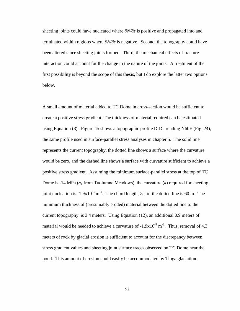
52
sheeting joints could have nucleated where ∂N/∂z is positive and propagated into and
terminated within regions where ∂N/∂z is negative. Second, the topography could have
been altered since sheeting joints formed. Third, the mechanical effects of fracture
interaction could account for the change in the nature of the joints. A treatment of the
first possibility is beyond the scope of this thesis, but I do explore the latter two options
below.
A small amount of material added to TC Dome in cross-section would be sufficient to
create a positive stress gradient. The thickness of material required can be estimated
using Equation (8). Figure 45 shows a topographic profile D-D' trending N60E (Fig. 24),
the same profile used in surface-parallel stress analyses in chapter 5. The solid line
represents the current topography, the dotted line shows a surface where the curvature
would be zero, and the dashed line shows a surface with curvature sufficient to achieve a
positive stress gradient. Assuming the minimum surface-parallel stress at the top of TC
Dome is -14 MPa (σ1 from Tuolumne Meadows), the curvature (k) required for sheeting
joint nucleation is -1.9x10⁻³
m-1
. The chord length, 2c, of the dotted line is 60 m. The
minimum thickness of (presumably eroded) material between the dotted line to the
current topography is 3.4 meters. Using Equation (12), an additional 0.9 meters of
material would be needed to achieve a curvature of -1.9x10⁻³
m-1
. Thus, removal of 4.3
meters of rock by glacial erosion is sufficient to account for the discrepancy between
stress gradient values and sheeting joint surface traces observed on TC Dome near the
pond. This amount of erosion could easily be accommodated by Tioga glaciation.
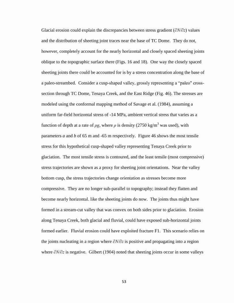
53
Glacial erosion could explain the discrepancies between stress gradient (∂N/∂z) values
and the distribution of sheeting joint traces near the base of TC Dome. They do not,
however, completely account for the nearly horizontal and closely spaced sheeting joints
oblique to the topographic surface there (Figs. 16 and 18). One way the closely spaced
sheeting joints there could be accounted for is by a stress concentration along the base of
a paleo-streambed. Consider a cusp-shaped valley, grossly representing a “paleo" cross-
section through TC Dome, Tenaya Creek, and the East Ridge (Fig. 46). The stresses are
modeled using the conformal mapping method of Savage et al. (1984), assuming a
uniform far-field horizontal stress of -14 MPa, ambient vertical stress that varies as a
function of depth at a rate of ρg, where ρ is density (2750 kg/m3 was used), with
parameters a and b of 65 m and -65 m respectively. Figure 46 shows the most tensile
stress for this hypothetical cusp-shaped valley representing Tenaya Creek prior to
glaciation. The most tensile stress is contoured, and the least tensile (most compressive)
stress trajectories are shown as a proxy for sheeting joint orientations. Near the valley
bottom cusp, the stress trajectories change orientation as stresses become more
compressive. They are no longer sub-parallel to topography; instead they flatten and
become nearly horizontal. like the sheeting joints do now. The joints thus might have
formed in a stream-cut valley that was convex on both sides prior to glaciation. Erosion
along Tenaya Creek, both glacial and fluvial, could have exposed sub-horizontal joints
formed earlier. Fluvial erosion could have exploited fracture F1. This scenario relies on
the joints nucleating in a region where ∂N/∂z is positive and propagating into a region
where ∂N/∂z is negative. Gilbert (1904) noted that sheeting joints occur in some valleys
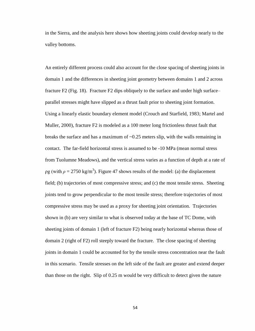
54
in the Sierra, and the analysis here shows how sheeting joints could develop nearly to the
valley bottoms.
An entirely different process could also account for the close spacing of sheeting joints in
domain 1 and the differences in sheeting joint geometry between domains 1 and 2 across
fracture F2 (Fig. 18). Fracture F2 dips obliquely to the surface and under high surface–
parallel stresses might have slipped as a thrust fault prior to sheeting joint formation.
Using a linearly elastic boundary element model (Crouch and Starfield, 1983; Martel and
Muller, 2000), fracture F2 is modeled as a 100 meter long frictionless thrust fault that
breaks the surface and has a maximum of ~0.25 meters slip, with the walls remaining in
contact. The far-field horizontal stress is assumed to be -10 MPa (mean normal stress
from Tuolumne Meadows), and the vertical stress varies as a function of depth at a rate of
ρg (with ρ = 2750 kg/m3). Figure 47 shows results of the model: (a) the displacement
field; (b) trajectories of most compressive stress; and (c) the most tensile stress. Sheeting
joints tend to grow perpendicular to the most tensile stress; therefore trajectories of most
compressive stress may be used as a proxy for sheeting joint orientation. Trajectories
shown in (b) are very similar to what is observed today at the base of TC Dome, with
sheeting joints of domain 1 (left of fracture F2) being nearly horizontal whereas those of
domain 2 (right of F2) roll steeply toward the fracture. The close spacing of sheeting
joints in domain 1 could be accounted for by the tensile stress concentration near the fault
in this scenario. Tensile stresses on the left side of the fault are greater and extend deeper
than those on the right. Slip of 0.25 m would be very difficult to detect given the nature
55
of the outcrops and markers near F2. Similar effects could be achieved with an even
shorter fault with less slip.
Geologic evidence suggests that sufficient time for topographic modification has elapsed
since sheeting joints near the pond formed. Glacial polish on the surface of some
sheeting joints at TC Dome indicates that at least some of them formed, and were
uncovered, prior to the retreat of Tioga glaciation, ~ 13,000 years ago (Clark, 1995).
Fracture F1 and the closely spaced sheeting joints make the region near the pond
particularly susceptible to glacial and fluvial erosion.
7.4 Other lessons
My research illuminated two other important points. First, filtering of the LIDAR data
was essential to calculate curvatures relevant to this project. Otherwise the curvatures
were dominated by short wavelength effects that would be regarded as “noise”. Second,
although sheeting joints have been noted for more than a century (Gilbert, 1904) as being
characteristically curved, their curvature was never measured. The sheeting joints at TC
Dome have curvatures with absolute values as great as ~4x10⁻³ m-1
over lengths of a few
tens of meters.
7.5 Suggestions for future work
The stress analyses for this project are based on the nearest stress measurement (Cadman,
1969), at Tuolumne Meadows ~ 11 km away from TC Dome. This measurement is the
only one within Tenaya Lake region. Additional stress measurements could greatly
56
enhance the project. If additional stress measurements were made available, one might
use a mechanical numerical model to help interpolate the stresses in the region.
The approach applied at TC Dome could be extended to other areas. Research-grade
aerial LIDAR data have been collected across the whole 77 km2 Tenaya Lake region by
NCALM. NCALM also has collected aerial LIDAR data across other regions of
Yosemite for the National Park Service. Analyses similar to those presented in this thesis
could be performed for these regions. Hundreds of photographs have been taken, by the
author and others, of the topography and individual sheeting joints in the Tenaya Lake
region. A map marking the location where many of these photographs were taken has
been made by the author in ArcGIS along with a database that could be useful for future
analyses. High-resolution topographic contour and hillshade digital elevation maps at a
scale of 1:10,000 have also been made by the author, based on aerial LIDAR data gridded
to 1 m resolution, for the entire Tenaya Lake region.
At least six specific locations are suggested for further study in the Tenaya Lake region:
1) The ridge containing the quarry near the road to May Lake, 2) Tenaya Canyon, 3)
Olmsted Point, 4) the bowl immediately north of Olmsted Point, 5) the ridge immediately
east of Olmsted Point, and 6) a dome above the southwest shore of Tenaya Lake (Fig. 5).
Data available for the quarry include: terrestrial LIDAR data collected by NCALM,
photographs, slab thickness measurements, and strike and dip measurements collected by
the author. Tenaya Canyon is an ideal place to study the effects of curvature on sheeting
joint formation because so few sheeting joints exist there. The bowl across Tioga Road
57
from Olmsted Point features displays numerous sheeting joints. High resolution (~ 5-7
cm) tripod-mounted LIDAR data were collected at the bowl by Ole Kaven (Stanford) and
Nicholas VanDerElst (UC Santa Cruz) using equipment loaned by Emily Brodsky (UC
Santa Cruz). The ridge east of Olmsted Point displays large sheeting joints with a unique
geometry on its NW slope. Further study of this ridge may yield insight into the
propagation and bifurcation of individual sheeting joints. Finally, the dome (elev. 2491
m) just east of Tenaya Lake has many sheeting joints. Sheeting joints there could be
mapped and characterized easily. The suggested study locations include each of the
major topographic features: domes (Olmsted Point), ridges (quarry and ridge east of
Olmsted Point), saddles (one at the top of a bowl 0.7 km north of Olmsted Point and one
along Tenaya Canyon), bowls (0.7 km north of Olmsted Point), and valleys (Tenaya
Canyon).
Although the aerial LIDAR data set was collected specifically to test the hypothesis
presented in this thesis, it could be used in many other ways. For example,
geomorphologists could use these data to explore glacial extent, ice volume, and fluvial
geomorphology. Structural geologists could examine the long bedrock fractures easily
seen in the data set as well.
7.6 Conclusions
The hypothesis that sheeting joints open in tension as a result of high, surface-parallel
compressive stresses acting parallel to a convex topographic surface is supported by field
evidence in Tenaya Lake region. The presence of sheeting joints on domes, ridges, and
58
saddles less than 1 km long indicate local topographic control of the joints rather than
regional topographic control because the local topographic curvature is sufficient for
sheeting joints to form, whereas the regional curvature is not. The presence of hackles on
sheeting joint faces and the lack of slip across features cut by sheeting joints (e.g., dikes,
veins, xenoliths, phenocrysts, and fractures) indicates that sheeting joints are tensile
fractures. The general lack of chemical alteration on sheeting joint faces suggests that
sheeting joints do not open from fluid pressure, but rather from a tension induced by high
compressive stresses acting parallel to a curved topographic surface. Further evidence of
high, surface-parallel compressive stresses is present in the form of buckled sheeting joint
slabs. Measurements by Cadman (1969) and Hickman (personal communication, 3/2008)
indicate that surface-parallel stresses are highly compressive (on the order of -10 MPa) in
the Yosemite region. The study area is on the verge of nucleating additional sheeting
joints given stresses of this magnitude and the curvature and slope of the topography.
The presence of many sheeting joints at TC Dome study area is consistent with modern
topographic and stress conditions. Compressive stresses parallel to the surface are likely
to have absolute magnitudes of at least 14 MPa and could be as high as 25 MPa. The
upper portion of TC Dome is doubly-convex; however much of the lower surface is
saddle-shaped, likely the result of glacial erosion. Sheeting joints at the lower portion of
TC Dome requires no more than 4.3 meters of erosion of the topographic surface since
the joints formed. Glacial erosion could have accomplished this.
59
The sheeting joint distribution everywhere at TC Dome cannot be accounted for entirely
by current topographic and regional stress conditions. The sheeting joints on the doubly
convex upper portions of the dome can be accounted for, both in terms of their
distribution and the orientation parallel to topography. Current topography and stress
conditions do not account for sheeting joints at the base of the dome in domains 1 and 2.
Sheeting joints of domain 1 are closely spaced, nearly horizontal, and are oblique to the
topographic surface. In domain 2, sheeting joints have an unusual geometry, dipping
steeply towards fracture F2. Both differences can be accounted for by plausible local
stress variations and erosion. The nearly horizontal sheeting joints in domain 1 can be
accounted for, at least in part, if the topography across Tenaya Creek were doubly convex
when the joints formed. The stress trajectories beneath a cusp-shaped valley are
consistent with sub-horizontal sheeting joints develop near the cusp. With a few meters
of glacial and stream erosion, the flat sheeting joints would be exposed. The close
spacing of sheeting joints in domain 1 and unusual geometry in domain 2 can be
accounted for if fracture F2 were activated as a thrust fault prior to sheeting joint
formation. A tensile stress concentration caused by the fault could account for the
closely spaced sheeting joints in domain 1. Trajectories of most compressive stress (a
proxy for sheeting joint orientation) roll toward the fault, thus accounting for the sheeting
joints in domain 2 steeply dipping toward fracture F2. Subtle geologic factors and
topographic modification need to be considered to account for the sheeting joints low on
TC Dome; presumably they would need to be considered in other places as well.
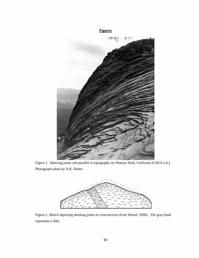
60
Figures
Figure 1. Sheeting joints sub-parallel to topography on Shuteye Peak, California (USGS n.d.).
Photograph taken by N.K. Huber.
Figure 2. Sketch depicting sheeting joints in cross-section (from Martel, 2006). The gray band
represents a dike.
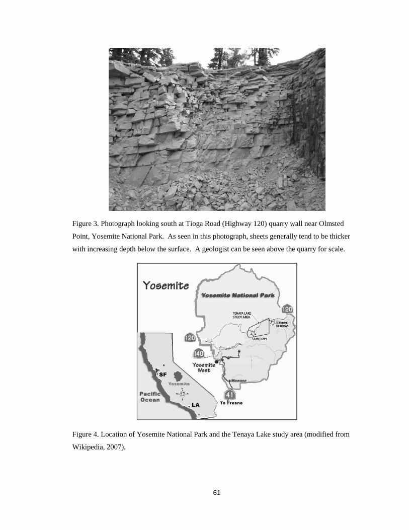
61
Figure 3. Photograph looking south at Tioga Road (Highway 120) quarry wall near Olmsted
Point, Yosemite National Park. As seen in this photograph, sheets generally tend to be thicker
with increasing depth below the surface. A geologist can be seen above the quarry for scale.
Figure 4. Location of Yosemite National Park and the Tenaya Lake study area (modified from
Wikipedia, 2007).
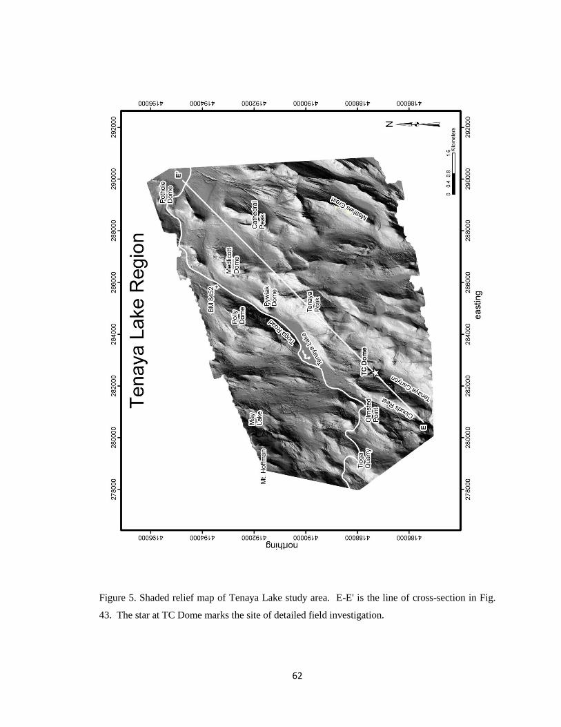
62
Figure 5. Shaded relief map of Tenaya Lake study area. E-E' is the line of cross-section in Fig.
43. The star at TC Dome marks the site of detailed field investigation.
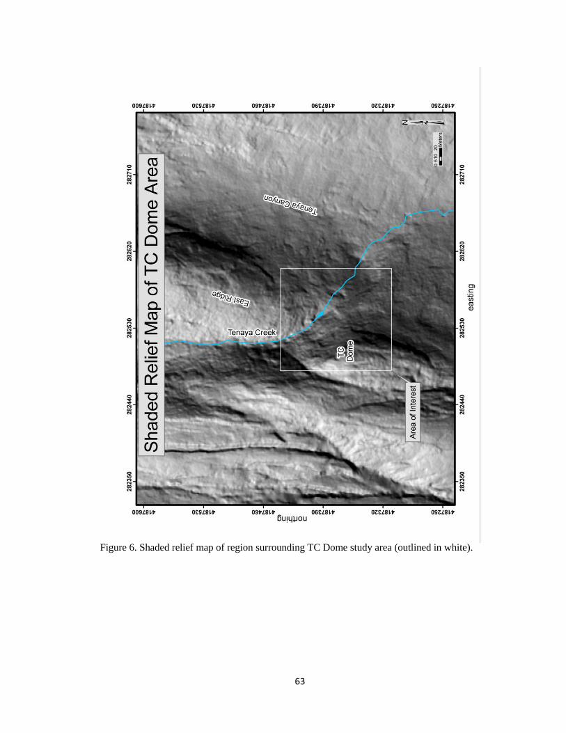
63
Figure 6. Shaded relief map of region surrounding TC Dome study area (outlined in white).
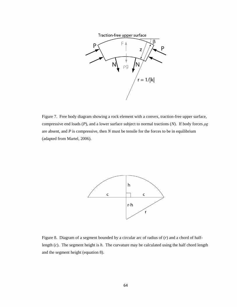
64
Figure 7. Free body diagram showing a rock element with a convex, traction-free upper surface,
compressive end loads (P), and a lower surface subject to normal tractions (N). If body forces ρg
are absent, and P is compressive, then N must be tensile for the forces to be in equilibrium
(adapted from Martel, 2006).
Figure 8. Diagram of a segment bounded by a circular arc of radius of (r) and a chord of half-
length (c). The segment height is h. The curvature may be calculated using the half chord length
and the segment height (equation 8).
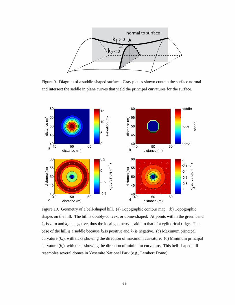
65
Figure 9. Diagram of a saddle-shaped surface. Gray planes shown contain the surface normal
and intersect the saddle in plane curves that yield the principal curvatures for the surface.
Figure 10. Geometry of a bell-shaped hill. (a) Topographic contour map. (b) Topographic
shapes on the hill. The hill is doubly-convex, or dome-shaped. At points within the green band
k1 is zero and k2 is negative, thus the local geometry is akin to that of a cylindrical ridge. The
base of the hill is a saddle because k1 is positive and k2 is negative. (c) Maximum principal
curvature (k1), with ticks showing the direction of maximum curvature. (d) Minimum principal
curvature (k2), with ticks showing the direction of minimum curvature. This bell-shaped hill
resembles several domes in Yosemite National Park (e.g., Lembert Dome).
a
c d
b
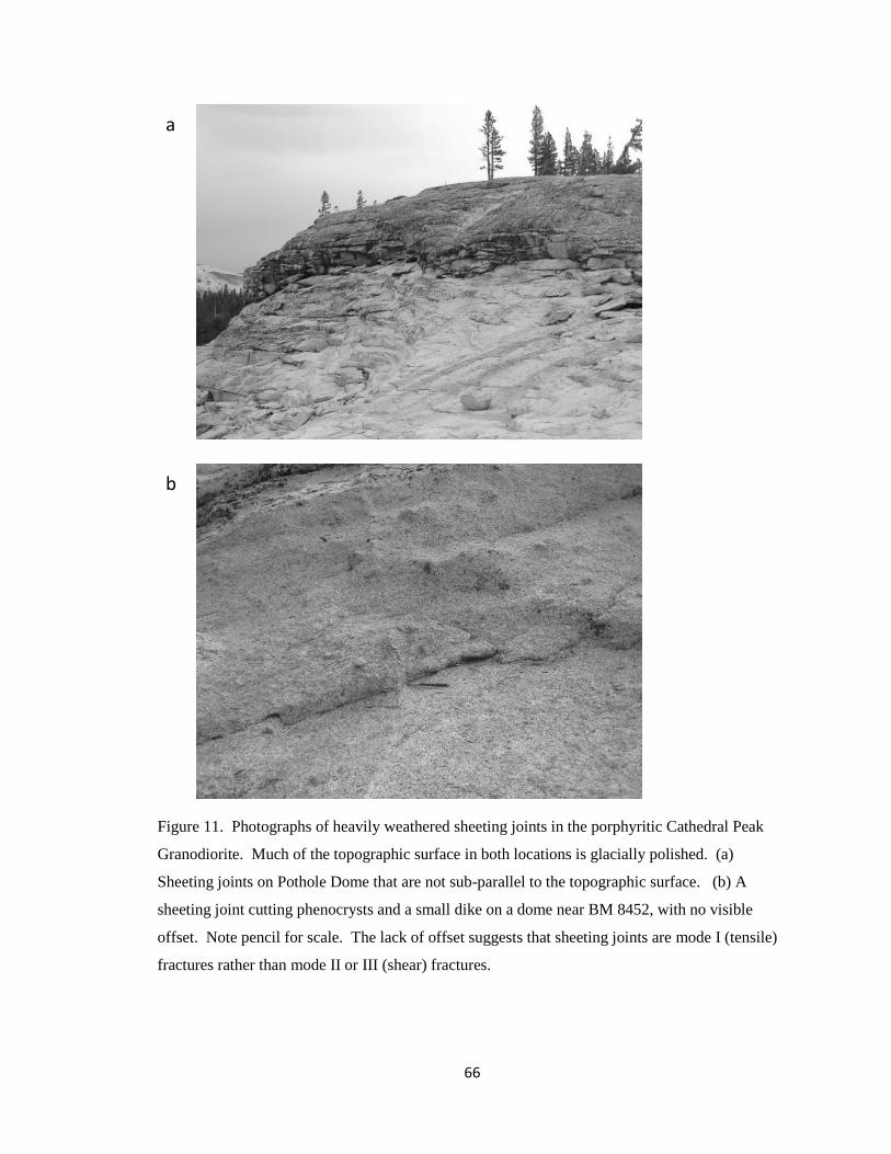
66
Figure 11. Photographs of heavily weathered sheeting joints in the porphyritic Cathedral Peak
Granodiorite. Much of the topographic surface in both locations is glacially polished. (a)
Sheeting joints on Pothole Dome that are not sub-parallel to the topographic surface. (b) A
sheeting joint cutting phenocrysts and a small dike on a dome near BM 8452, with no visible
offset. Note pencil for scale. The lack of offset suggests that sheeting joints are mode I (tensile)
fractures rather than mode II or III (shear) fractures.
a
b
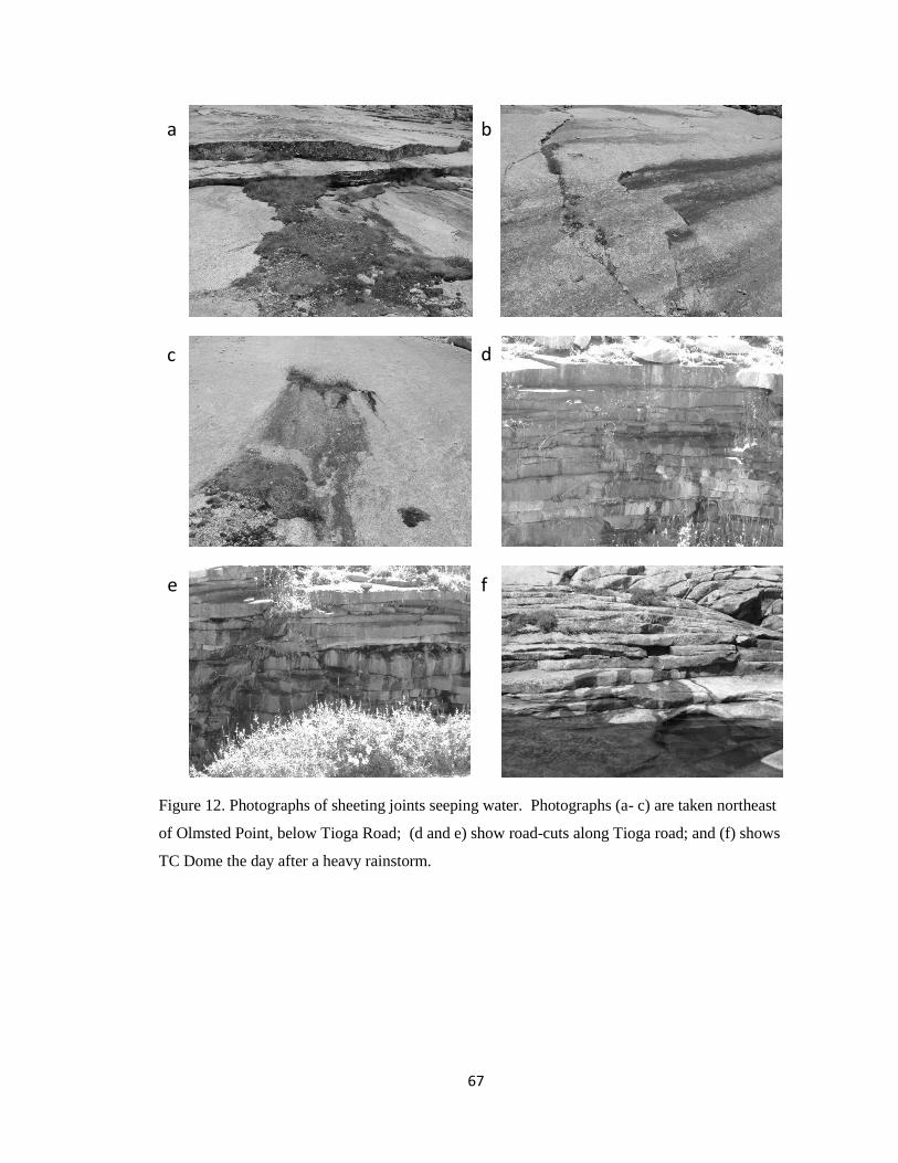
67
Figure 12. Photographs of sheeting joints seeping water. Photographs (a- c) are taken northeast
of Olmsted Point, below Tioga Road; (d and e) show road-cuts along Tioga road; and (f) shows
TC Dome the day after a heavy rainstorm.
a b
d c
e f
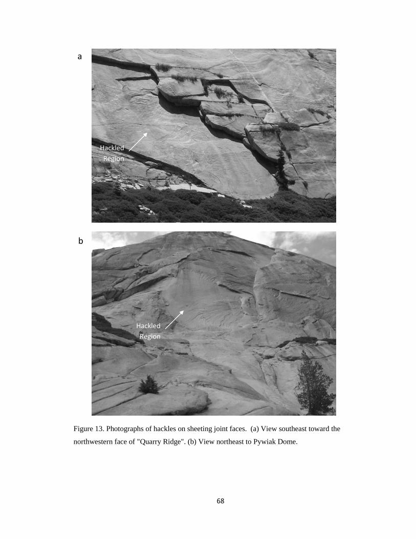
68
Figure 13. Photographs of hackles on sheeting joint faces. (a) View southeast toward the
northwestern face of "Quarry Ridge". (b) View northeast to Pywiak Dome.
Hackled
Region
Hackled
Region
b
a
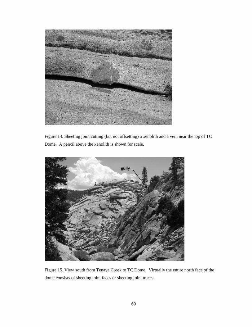
69
Figure 14. Sheeting joint cutting (but not offsetting) a xenolith and a vein near the top of TC
Dome. A pencil above the xenolith is shown for scale.
Figure 15. View south from Tenaya Creek to TC Dome. Virtually the entire north face of the
dome consists of sheeting joint faces or sheeting joint traces.
gully
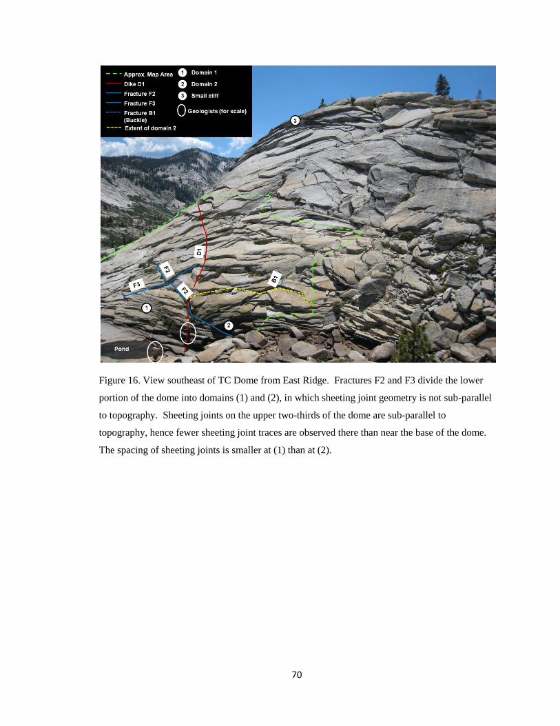
70
Figure 16. View southeast of TC Dome from East Ridge. Fractures F2 and F3 divide the lower
portion of the dome into domains (1) and (2), in which sheeting joint geometry is not sub-parallel
to topography. Sheeting joints on the upper two-thirds of the dome are sub-parallel to
topography, hence fewer sheeting joint traces are observed there than near the base of the dome.
The spacing of sheeting joints is smaller at (1) than at (2).

71
Figure 17. View northeast to East Ridge. The green line marks the approximate extent of fracture
map on Figure 20. Dike D1 extends further than shown. The east side of the ridge faces Tenaya
Canyon and displays extensive glacial polish. Sheets on the ridge tend to be more heavily
fractured than those on TC Dome.
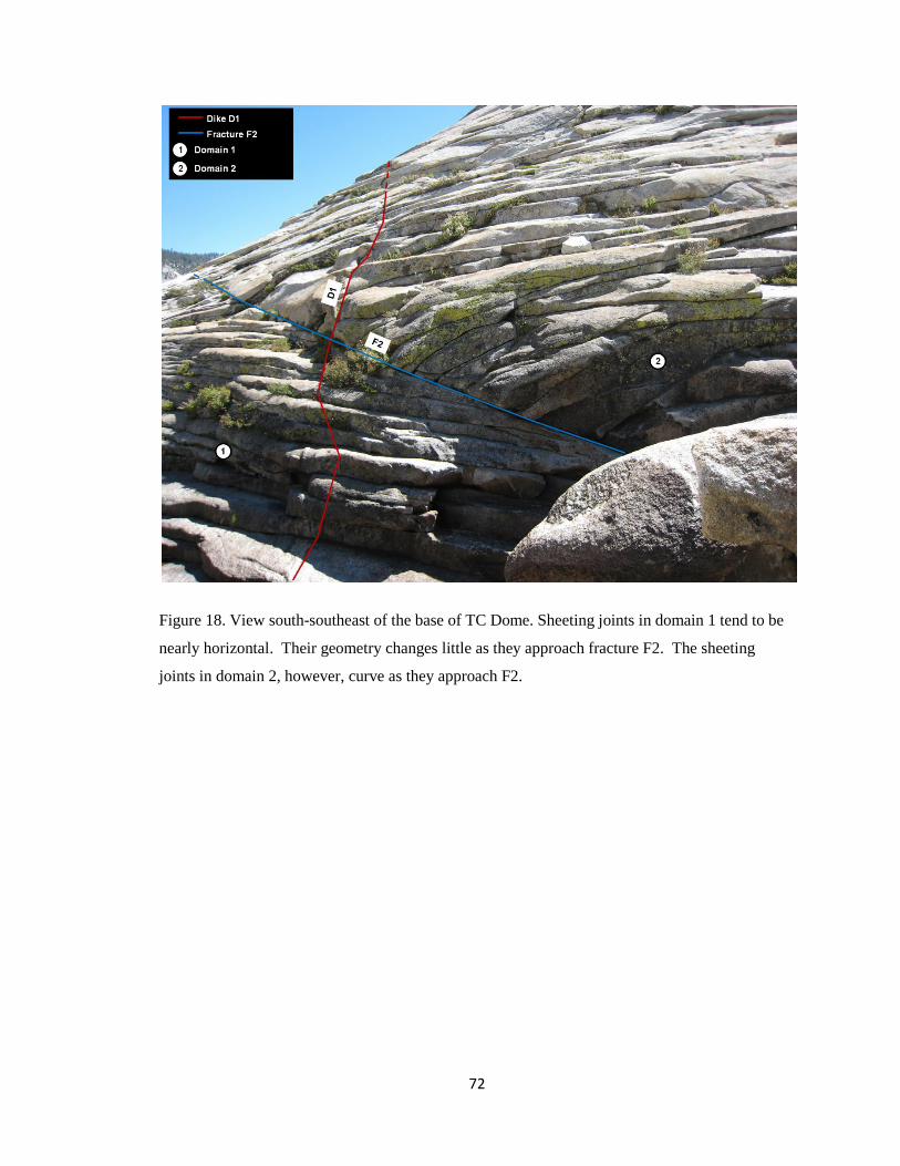
72
Figure 18. View south-southeast of the base of TC Dome. Sheeting joints in domain 1 tend to be
nearly horizontal. Their geometry changes little as they approach fracture F2. The sheeting
joints in domain 2, however, curve as they approach F2.
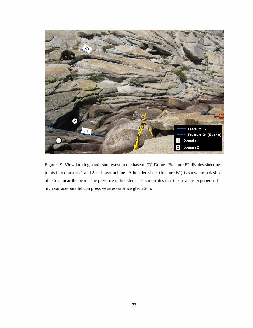
73
Figure 19. View looking south-southwest to the base of TC Dome. Fracture F2 divides sheeting
joints into domains 1 and 2 is shown in blue. A buckled sheet (fracture B1) is shown as a dashed
blue line, near the bear. The presence of buckled sheets indicates that the area has experienced
high surface-parallel compressive stresses since glaciation.
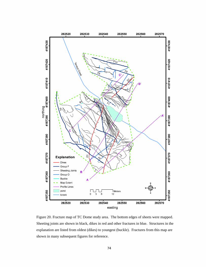
74
Figure 20. Fracture map of TC Dome study area. The bottom edges of sheets were mapped.
Sheeting joints are shown in black, dikes in red and other fractures in blue. Structures in the
explanation are listed from oldest (dikes) to youngest (buckle). Fractures from this map are
shown in many subsequent figures for reference.
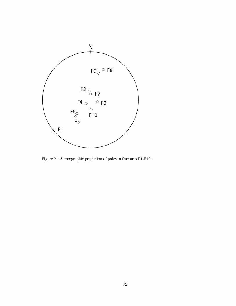
75
Figure 21. Stereographic projection of poles to fractures F1-F10.
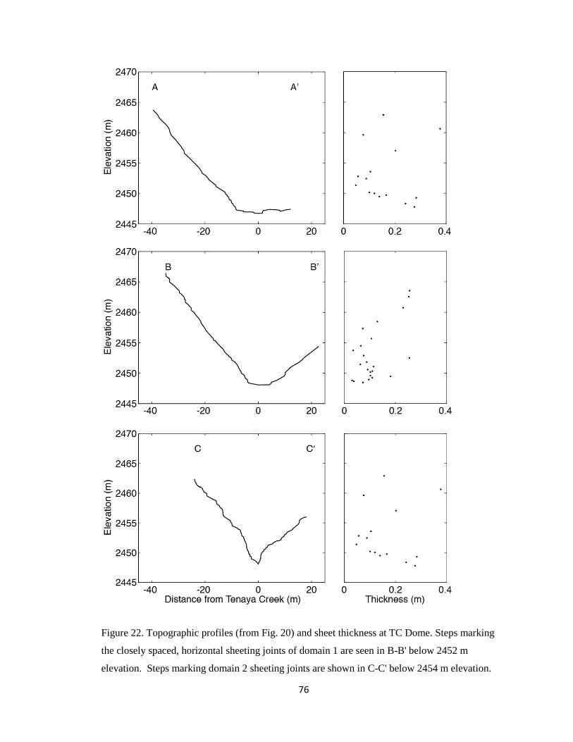
76
Figure 22. Topographic profiles (from Fig. 20) and sheet thickness at TC Dome. Steps marking
the closely spaced, horizontal sheeting joints of domain 1 are seen in B-B' below 2452 m
elevation. Steps marking domain 2 sheeting joints are shown in C-C' below 2454 m elevation.
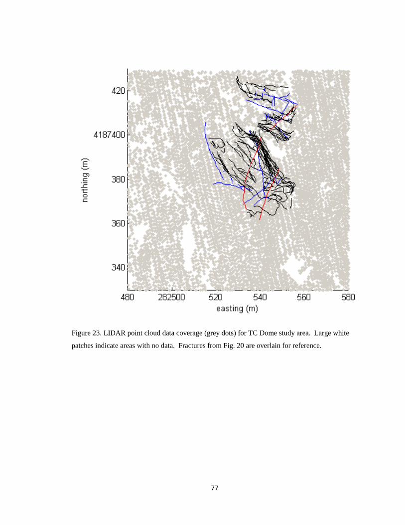
77
Figure 23. LIDAR point cloud data coverage (grey dots) for TC Dome study area. Large white
patches indicate areas with no data. Fractures from Fig. 20 are overlain for reference.
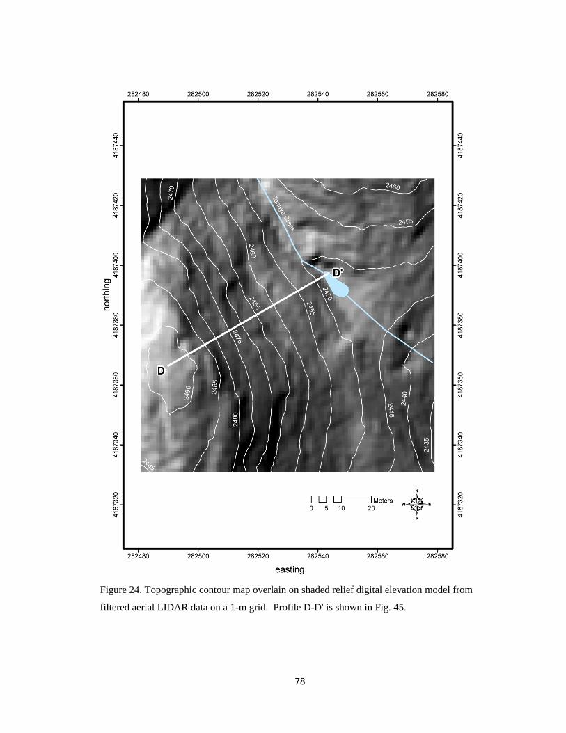
78
Figure 24. Topographic contour map overlain on shaded relief digital elevation model from
filtered aerial LIDAR data on a 1-m grid. Profile D-D' is shown in Fig. 45.
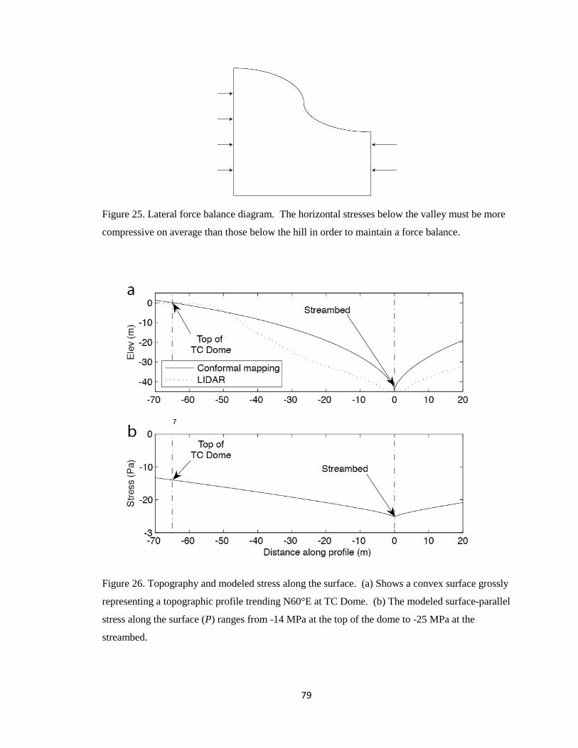
79
Figure 25. Lateral force balance diagram. The horizontal stresses below the valley must be more
compressive on average than those below the hill in order to maintain a force balance.
Figure 26. Topography and modeled stress along the surface. (a) Shows a convex surface grossly
representing a topographic profile trending N60°E at TC Dome. (b) The modeled surface-parallel
stress along the surface (P) ranges from -14 MPa at the top of the dome to -25 MPa at the
streambed.
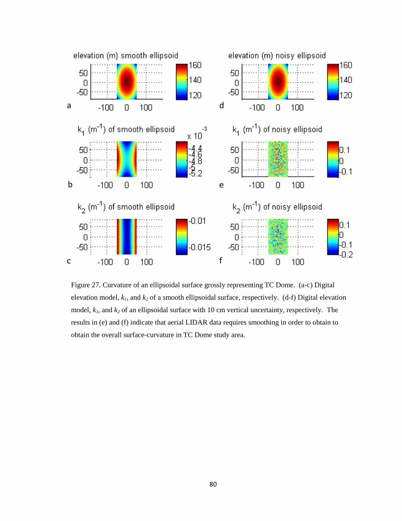
80
Figure 27. Curvature of an ellipsoidal surface grossly representing TC Dome. (a-c) Digital
elevation model, k1, and k2 of a smooth ellipsoidal surface, respectively. (d-f) Digital elevation
model, k1, and k2 of an ellipsoidal surface with 10 cm vertical uncertainty, respectively. The
results in (e) and (f) indicate that aerial LIDAR data requires smoothing in order to obtain to
obtain the overall surface-curvature in TC Dome study area.
a
b
c
d
e
f
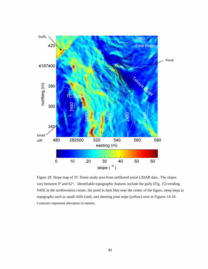
81
Figure 28. Slope map of TC Dome study area from unfiltered aerial LIDAR data. The slopes
vary between 0° and 62°. Identifiable topographic features include the gully (Fig. 15) trending
N45E in the northwestern corner, the pond in dark blue near the center of the figure, steep steps in
topography such as small cliffs (red), and sheeting joint steps (yellow) seen in Figures 14-18.
Contours represent elevation in meters.
Gully
Small
cliff
Pond
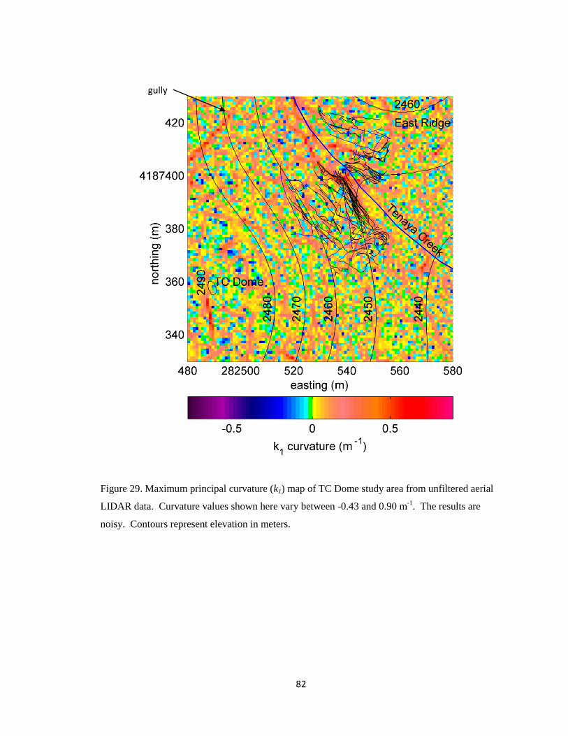
82
Figure 29. Maximum principal curvature (k1) map of TC Dome study area from unfiltered aerial
LIDAR data. Curvature values shown here vary between -0.43 and 0.90 m-1
. The results are
noisy. Contours represent elevation in meters.
gully
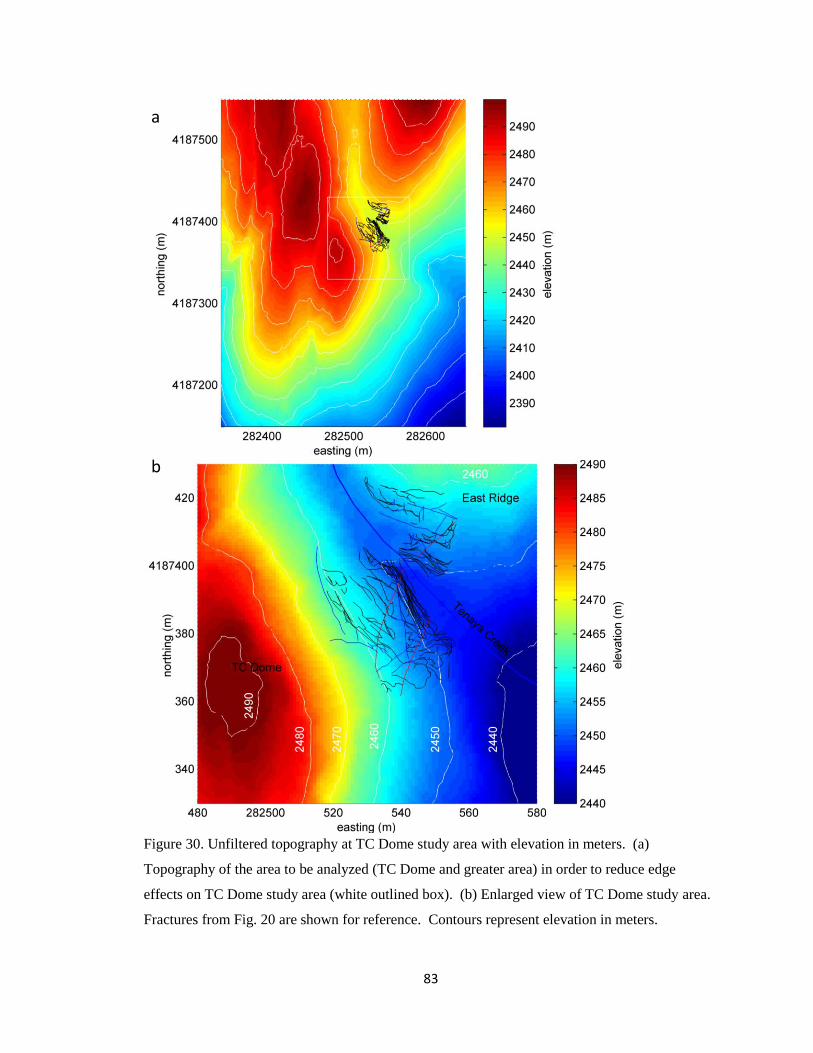
83
Figure 30. Unfiltered topography at TC Dome study area with elevation in meters. (a)
Topography of the area to be analyzed (TC Dome and greater area) in order to reduce edge
effects on TC Dome study area (white outlined box). (b) Enlarged view of TC Dome study area.
Fractures from Fig. 20 are shown for reference. Contours represent elevation in meters.
a
b
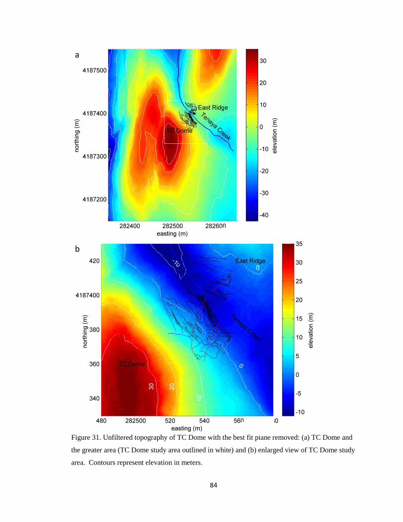
84
Figure 31. Unfiltered topography of TC Dome with the best fit plane removed: (a) TC Dome and
the greater area (TC Dome study area outlined in white) and (b) enlarged view of TC Dome study
area. Contours represent elevation in meters.
a
b
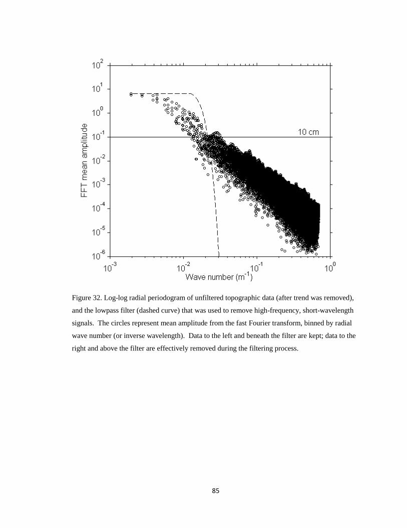
85
Figure 32. Log-log radial periodogram of unfiltered topographic data (after trend was removed),
and the lowpass filter (dashed curve) that was used to remove high-frequency, short-wavelength
signals. The circles represent mean amplitude from the fast Fourier transform, binned by radial
wave number (or inverse wavelength). Data to the left and beneath the filter are kept; data to the
right and above the filter are effectively removed during the filtering process.

86
Figure 33. Filtered and re-trended digital elevation map of TC Dome study area. The overall
topographic shape remains, but smaller features such as the gully (Fig. 15) are no longer visible.
Contours represent elevation in meters.
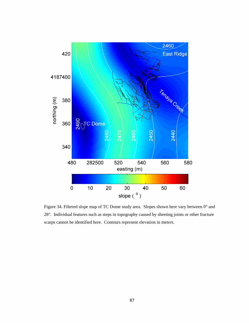
87
Figure 34. Filtered slope map of TC Dome study area. Slopes shown here vary between 0° and
28°. Individual features such as steps in topography caused by sheeting joints or other fracture
scarps cannot be identified here. Contours represent elevation in meters.
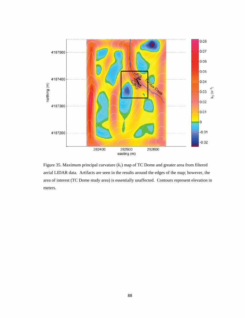
88
Figure 35. Maximum principal curvature (k1) map of TC Dome and greater area from filtered
aerial LIDAR data. Artifacts are seen in the results around the edges of the map; however, the
area of interest (TC Dome study area) is essentially unaffected. Contours represent elevation in
meters.
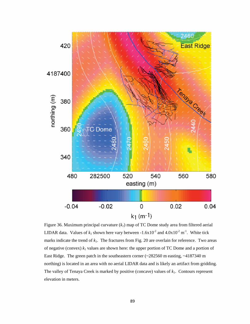
89
Figure 36. Maximum principal curvature (k1) map of TC Dome study area from filtered aerial
LIDAR data. Values of k1 shown here vary between -1.6x10⁻²
and 4.0x10⁻²
m-1
. White tick
marks indicate the trend of k1. The fractures from Fig. 20 are overlain for reference. Two areas
of negative (convex) k1 values are shown here: the upper portion of TC Dome and a portion of
East Ridge. The green patch in the southeastern corner (~282560 m easting, ~4187340 m
northing) is located in an area with no aerial LIDAR data and is likely an artifact from gridding.
The valley of Tenaya Creek is marked by positive (concave) values of k1. Contours represent
elevation in meters.
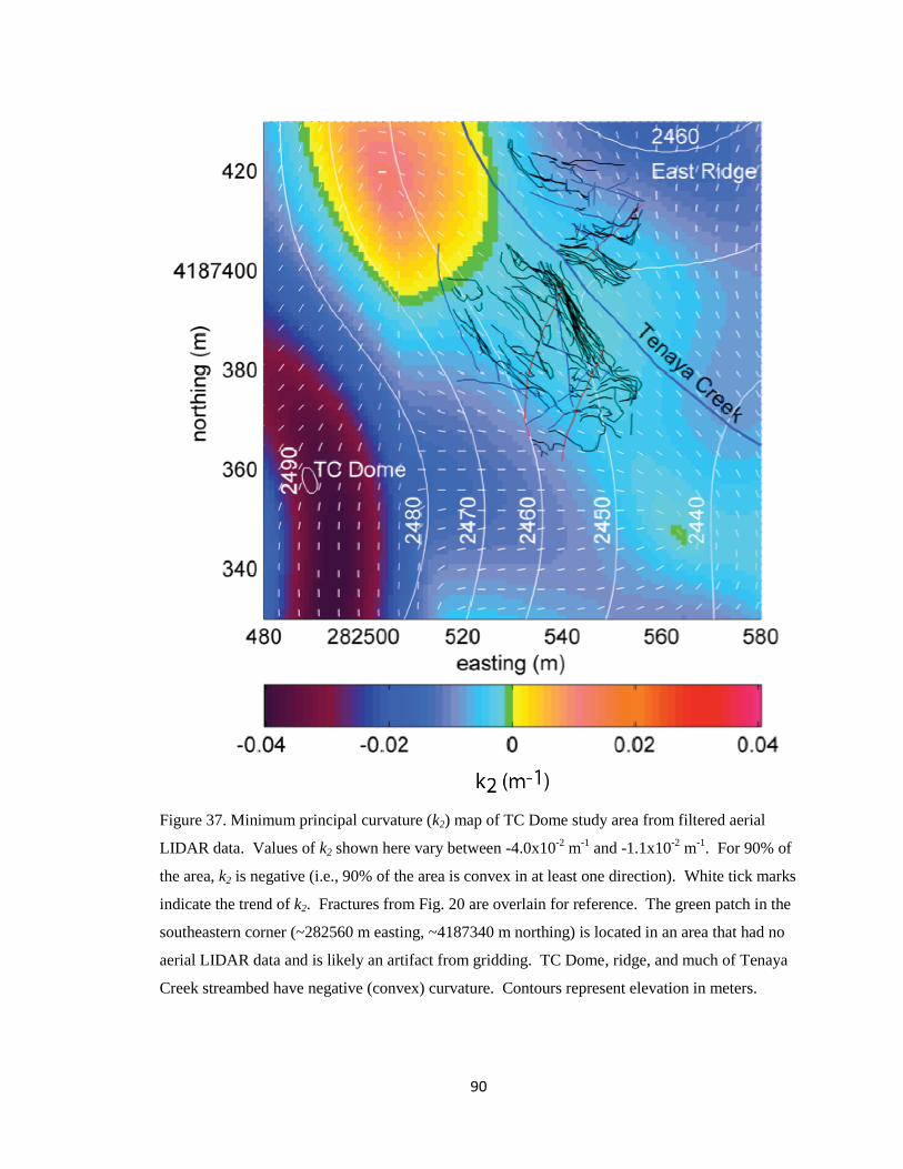
90
Figure 37. Minimum principal curvature (k2) map of TC Dome study area from filtered aerial
LIDAR data. Values of k2 shown here vary between -4.0x10⁻²
m-1
and -1.1x10⁻²
m-1
. For 90% of
the area, k2 is negative (i.e., 90% of the area is convex in at least one direction). White tick marks
indicate the trend of k2. Fractures from Fig. 20 are overlain for reference. The green patch in the
southeastern corner (~282560 m easting, ~4187340 m northing) is located in an area that had no
aerial LIDAR data and is likely an artifact from gridding. TC Dome, ridge, and much of Tenaya
Creek streambed have negative (convex) curvature. Contours represent elevation in meters.
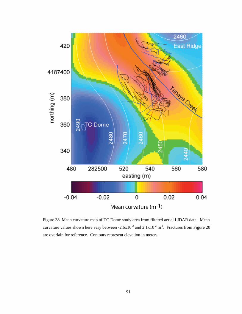
91
Figure 38. Mean curvature map of TC Dome study area from filtered aerial LIDAR data. Mean
curvature values shown here vary between -2.6x10⁻²
and 2.1x10⁻²
m-1
. Fractures from Figure 20
are overlain for reference. Contours represent elevation in meters.
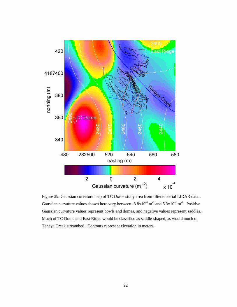
92
Figure 39. Gaussian curvature map of TC Dome study area from filtered aerial LIDAR data.
Gaussian curvature values shown here vary between -3.8x10⁻⁴
m-2
and 5.3x10⁻⁴
m-2
. Positive
Gaussian curvature values represent bowls and domes, and negative values represent saddles.
Much of TC Dome and East Ridge would be classified as saddle-shaped, as would much of
Tenaya Creek streambed. Contours represent elevation in meters.
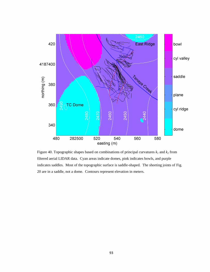
93
Figure 40. Topographic shapes based on combinations of principal curvatures k1 and k2 from
filtered aerial LIDAR data. Cyan areas indicate domes, pink indicates bowls, and purple
indicates saddles. Most of the topographic surface is saddle-shaped. The sheeting joints of Fig.
20 are in a saddle, not a dome. Contours represent elevation in meters.
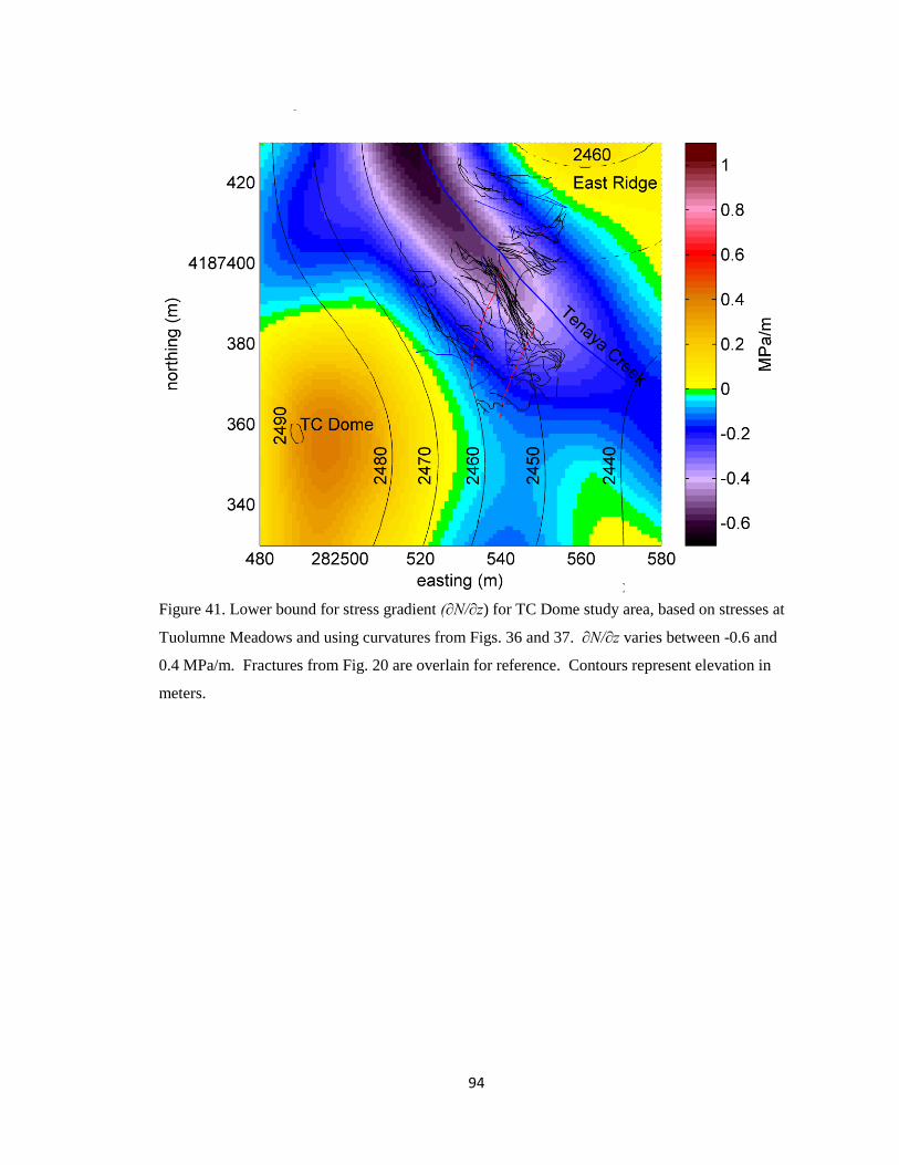
94
Figure 41. Lower bound for stress gradient (∂N/∂z) for TC Dome study area, based on stresses at
Tuolumne Meadows and using curvatures from Figs. 36 and 37. ∂N/∂z varies between -0.6 and
0.4 MPa/m. Fractures from Fig. 20 are overlain for reference. Contours represent elevation in
meters.
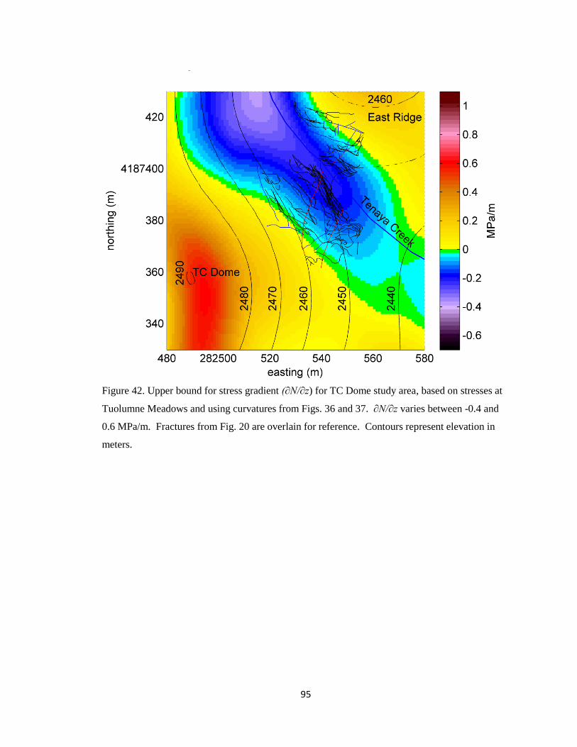
95
Figure 42. Upper bound for stress gradient (∂N/∂z) for TC Dome study area, based on stresses at
Tuolumne Meadows and using curvatures from Figs. 36 and 37. ∂N/∂z varies between -0.4 and
0.6 MPa/m. Fractures from Fig. 20 are overlain for reference. Contours represent elevation in
meters.
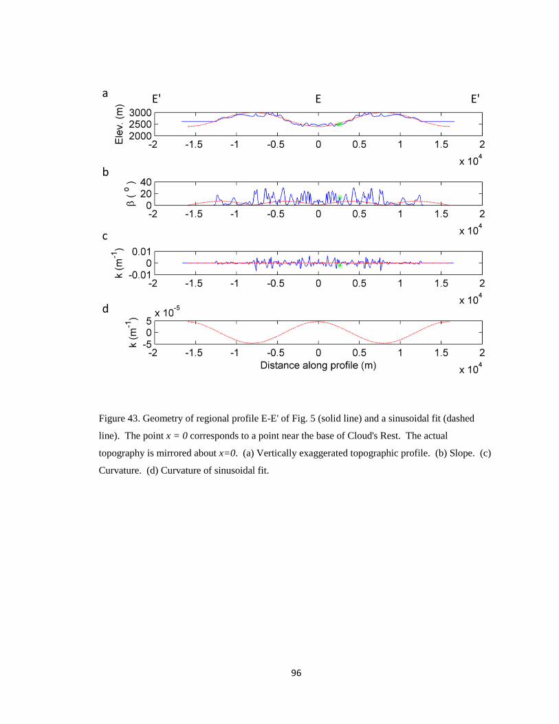
96
Figure 43. Geometry of regional profile E-E' of Fig. 5 (solid line) and a sinusoidal fit (dashed
line). The point x = 0 corresponds to a point near the base of Cloud's Rest. The actual
topography is mirrored about x=0. (a) Vertically exaggerated topographic profile. (b) Slope. (c)
Curvature. (d) Curvature of sinusoidal fit.
a
b
c
d
E E' E'
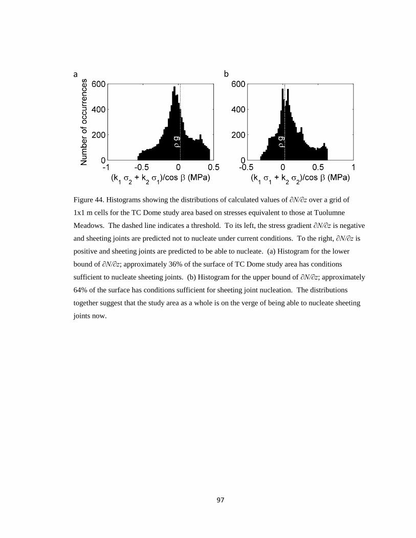
97
Figure 44. Histograms showing the distributions of calculated values of ∂N/∂z over a grid of
1x1 m cells for the TC Dome study area based on stresses equivalent to those at Tuolumne
Meadows. The dashed line indicates a threshold. To its left, the stress gradient ∂N/∂z is negative
and sheeting joints are predicted not to nucleate under current conditions. To the right, ∂N/∂z is
positive and sheeting joints are predicted to be able to nucleate. (a) Histogram for the lower
bound of ∂N/∂z; approximately 36% of the surface of TC Dome study area has conditions
sufficient to nucleate sheeting joints. (b) Histogram for the upper bound of ∂N/∂z; approximately
64% of the surface has conditions sufficient for sheeting joint nucleation. The distributions
together suggest that the study area as a whole is on the verge of being able to nucleate sheeting
joints now.
a b
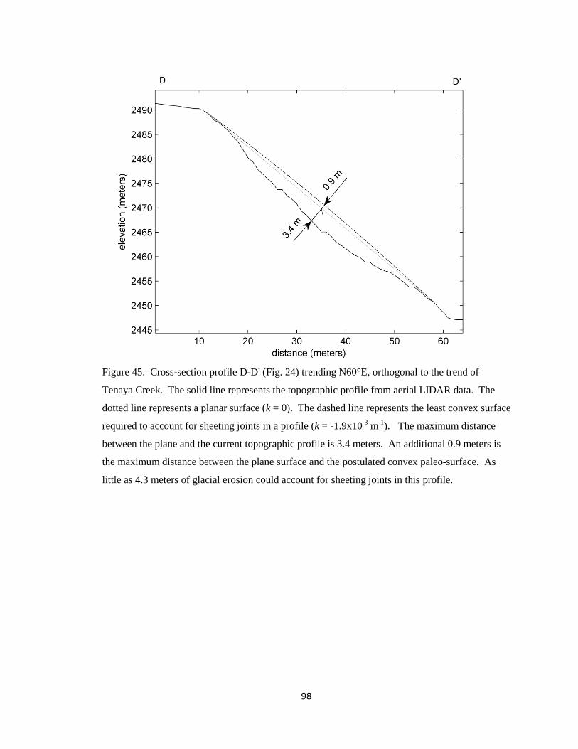
98
Figure 45. Cross-section profile D-D' (Fig. 24) trending N60°E, orthogonal to the trend of
Tenaya Creek. The solid line represents the topographic profile from aerial LIDAR data. The
dotted line represents a planar surface (k = 0). The dashed line represents the least convex surface
required to account for sheeting joints in a profile (k = -1.9x10⁻³
m-1
). The maximum distance
between the plane and the current topographic profile is 3.4 meters. An additional 0.9 meters is
the maximum distance between the plane surface and the postulated convex paleo-surface. As
little as 4.3 meters of glacial erosion could account for sheeting joints in this profile.
D D'
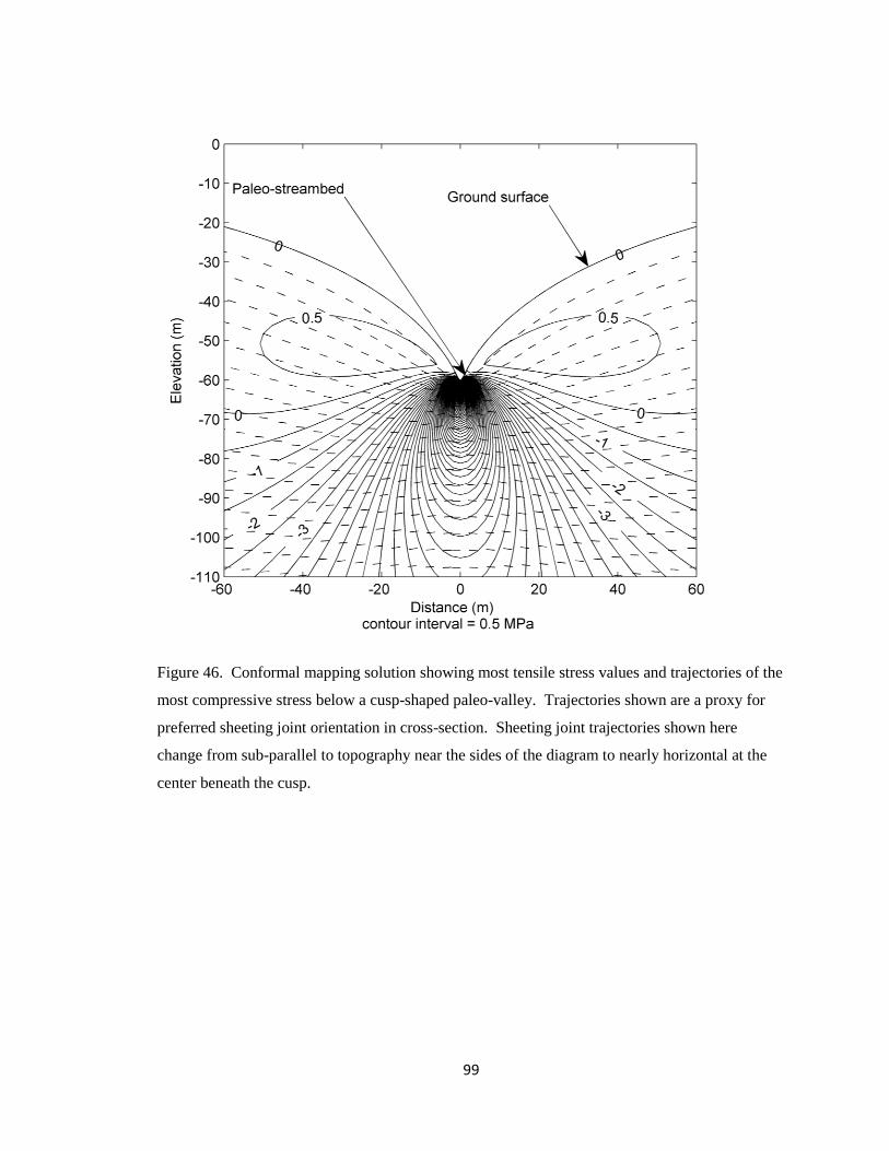
99
Figure 46. Conformal mapping solution showing most tensile stress values and trajectories of the
most compressive stress below a cusp-shaped paleo-valley. Trajectories shown are a proxy for
preferred sheeting joint orientation in cross-section. Sheeting joint trajectories shown here
change from sub-parallel to topography near the sides of the diagram to nearly horizontal at the
center beneath the cusp.
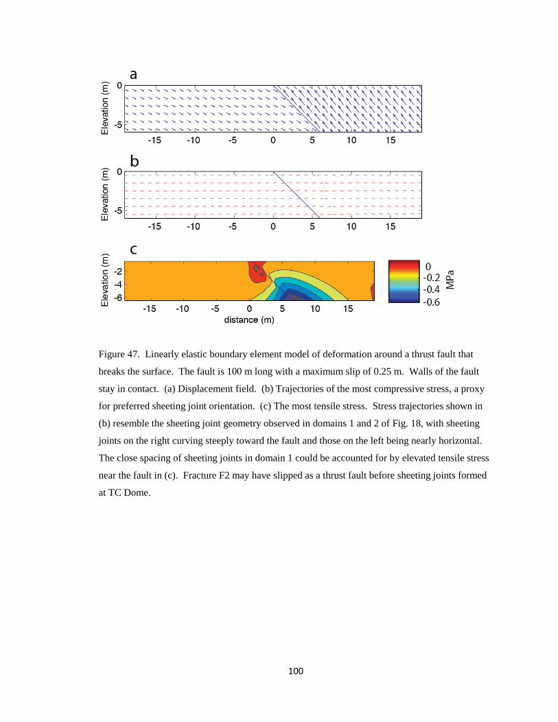
100
Figure 47. Linearly elastic boundary element model of deformation around a thrust fault that
breaks the surface. The fault is 100 m long with a maximum slip of 0.25 m. Walls of the fault
stay in contact. (a) Displacement field. (b) Trajectories of the most compressive stress, a proxy
for preferred sheeting joint orientation. (c) The most tensile stress. Stress trajectories shown in
(b) resemble the sheeting joint geometry observed in domains 1 and 2 of Fig. 18, with sheeting
joints on the right curving steeply toward the fault and those on the left being nearly horizontal.
The close spacing of sheeting joints in domain 1 could be accounted for by elevated tensile stress
near the fault in (c). Fracture F2 may have slipped as a thrust fault before sheeting joints formed
at TC Dome.

101
Appendix A: Orientation of Structural Features at TC Dome
Appendix A includes maps showing strike and dip of sheeting joint and fracture surfaces,
and the locations for which detailed notes are available. Two maps are included in this
appendix: A-1 shows the orientation data (strike and dip); A-2 shows locations for which
detailed notes are available in the database.
All data used to make these maps as well as the fracture map from Fig. 20 are available in
ASCII format (from myself or Dr. Martel) and include point names, location (northing,
easting, and elevation in meters), and any additional information (e.g., strike and dip or
other notes). Names are based upon the type of feature, the order in which it was
surveyed, and the point along the feature. For example: SJ28B corresponds to the 28th
sheeting joint surveyed, and the 2nd point (B) surveyed along that particular sheeting
joint. Dikes and planar fractures are named DIKE and FRAC respectively; CPT indicates
control points; and P indicates profile. For both the orientation data and the notes, the
names and locations listed are the nearest surveyed point, usually within 0.5 meters of the
actual strike and dip or location for which notes were taken.
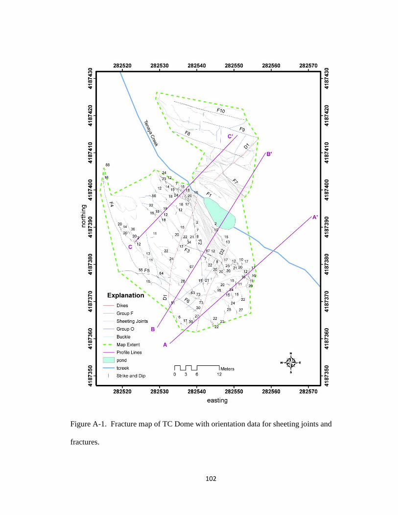
102
Figure A-1. Fracture map of TC Dome with orientation data for sheeting joints and
fractures.
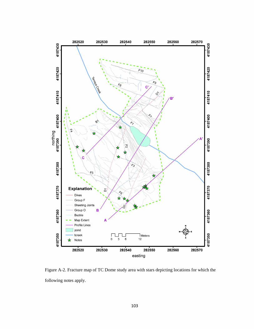
103
Figure A-2. Fracture map of TC Dome study area with stars depicting locations for which the
following notes apply.
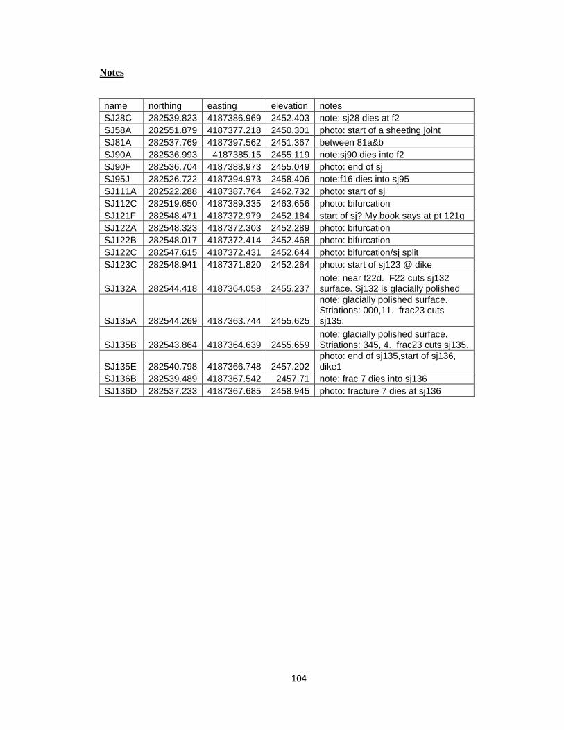
104
Notes
name northing easting elevation notes
SJ28C 282539.823 4187386.969 2452.403 note: sj28 dies at f2
SJ58A 282551.879 4187377.218 2450.301 photo: start of a sheeting joint
SJ81A 282537.769 4187397.562 2451.367 between 81a&b
SJ90A 282536.993 4187385.15 2455.119 note:sj90 dies into f2
SJ90F 282536.704 4187388.973 2455.049 photo: end of sj
SJ95J 282526.722 4187394.973 2458.406 note:f16 dies into sj95
SJ111A 282522.288 4187387.764 2462.732 photo: start of sj
SJ112C 282519.650 4187389.335 2463.656 photo: bifurcation
SJ121F 282548.471 4187372.979 2452.184 start of sj? My book says at pt 121g
SJ122A 282548.323 4187372.303 2452.289 photo: bifurcation
SJ122B 282548.017 4187372.414 2452.468 photo: bifurcation
SJ122C 282547.615 4187372.431 2452.644 photo: bifurcation/sj split
SJ123C 282548.941 4187371.820 2452.264 photo: start of sj123 @ dike
SJ132A 282544.418 4187364.058 2455.237 note: near f22d. F22 cuts sj132 surface. Sj132 is glacially polished
SJ135A 282544.269 4187363.744 2455.625
note: glacially polished surface. Striations: 000,11. frac23 cuts sj135.
SJ135B 282543.864 4187364.639 2455.659 note: glacially polished surface. Striations: 345, 4. frac23 cuts sj135.
SJ135E 282540.798 4187366.748 2457.202 photo: end of sj135,start of sj136, dike1
SJ136B 282539.489 4187367.542 2457.71 note: frac 7 dies into sj136
SJ136D 282537.233 4187367.685 2458.945 photo: fracture 7 dies at sj136

105
Appendix B: Sheet Curvature
Appendix B includes terrestrial (tripod-mounted) LIDAR data for TC Dome, and results
of the curvature analyses of two individual sheeting joint surfaces. LIDAR data were
collected by Ole Kaven (Stanford) and Nicholas VanDerElst (UC Santa Cruz) during the
summer of 2007 with equipment loaned by Emily Brodsky (UC Santa Cruz). The spot
spacing is approximately 5 cm. Figure B-1shows a hillshade digital elevation model of
TC Dome in map view, with the sheets of interest highlighted. Figure B-2 shows the
maximum and minimum principal curvatures of individual sheeting joint surfaces.
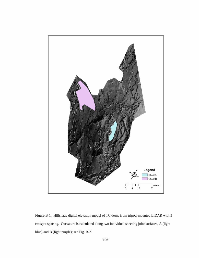
106
Figure B-1. Hillshade digital elevation model of TC dome from tripod-mounted LIDAR with 5
cm spot spacing. Curvature is calculated along two individual sheeting joint surfaces, A (light
blue) and B (light purple); see Fig. B-2.
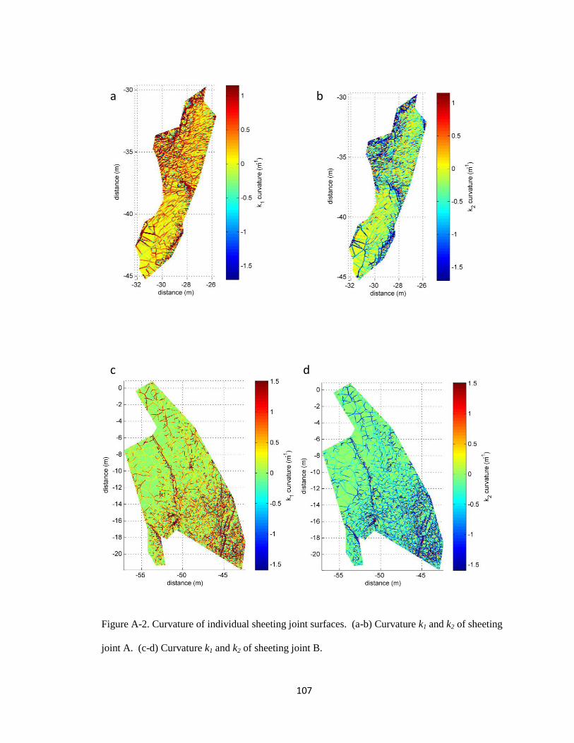
107
Figure A-2. Curvature of individual sheeting joint surfaces. (a-b) Curvature k1 and k2 of sheeting
joint A. (c-d) Curvature k1 and k2 of sheeting joint B.
a b
c d
108
References Cited
Bahat, D., Grossenbacher, K., and Karaski, K., 1999, Mechanism of exfoliation joint formation in
granitic rocks, Yosemite National Park: Journal of Structural Geology, v. 21, p. 85-96.
Bateman, P.C., and Wahrhaftig, C., 1966, Geology of the Sierra Nevada. In: Bailey, E.H. (Ed.),
Geology of Northern California (special issue): California Division of Mines and Geology
Bulletin, 190, p. 107-172.
Bergbauer, S., 2002, The use of curvature for the analysis of folding and fracturing with
application to the Emigrant Gap Anticline, Wyoming [PhD thesis]: Stanford University, 200 p.
Bergbauer, S., and Pollard, D.D., 2003, How to calculate normal curvatures of sampled
geological surfaces: Journal of Structural Geology, v. 25, p. 277–289.
Bradley, W.C., 1963, Large-scale exfoliation in massive sandstones of the Colorado Plateau:
Geological Society of America Bulletin, v. 74, p. 519–528.
Cadman, J., 1969, The origin of exfoliation joints in granitic rocks [Ph.D. thesis]: Berkeley,
University of California, 277 p.
Carmichael, R.S., 1989, Practical handbook of physical properties of rocks and minerals: Boca
Raton, Florida, CRC, 741 p.
Cassel, E.J., Graham, S.A., and Chamberlain, C.P., 2009, Cenozoic tectonic and topographic
evolution of the northern Sierra Nevada, California, through stable isotopic paleoaltimetry in
volcanic glass: Geology, v. 37, p. 547-550.
Chorley, R.J., Schumm, S.A., and Sugden, D.E., 1984, Geomorphology: London, Methuen, 605
p.
Clark, D.H., 1995, Extent, timing, and climatic significance of latest Pleistocene and Holocene
glaciation in the Sierra Nevada, California [Ph.D. thesis]: Seattle, Washington University, 191 p.
109
Coleman, D.S., Gray, W., Glazner, A.F., 2004, Rethinking the emplacement and evolution of
zoned plutons: Geochronologic evidence for incremental assembly for the Tuolumne Intrusive
Suite, California: Geology, v. 32, p. 433-436.
Crouch, S.L., and Starfield, A.M., 1983, Boundary element methods in solid mechanics: London,
Allen and Unwin, 334 p.
Dale, T.N., 1923, The commercial granites of New England: U.S. Geological Survey Bulletin,
738, 488 p.
Ericson, K., and Olvmo, M., 2004, A-tents in the central Sierra Nevada, California: a
geomorphological indicator of tectonic stress: Physical Geography, v. 25, p. 291-312.
Gilbert, G.K., 1904, Dome and dome structures of the High Sierra: Geological Society of
America Bulletin, v. 15, p. 29-36.
Gillespie, A.R., 1982, Quaternary glaciation and tectonism in the southeastern Sierra Nevada,
Inyo County, California [Ph. D. thesis]: Pasadena, California Institute of Technology, 695 p.
Glazner, A.F., Bartley, J.M., Coleman, D.S., Gray, W., and Taylor, R.Z., 2004, Are plutons
assembled over millions of years by amalgamation from small magma chambers?: GSA Today, v.
14, p. 4-11.
Goudie, A.S. (Ed.), 004, Encyclopedia of geomorphology: London, Rutledge, 1156 p.
Henry, C.D., 2009, Uplift of the Sierra Nevada, California: Geology, v. 37, p. 575-576.
Holman, W.R, 1976, The origin of sheeting joints: A hypothesis [Ph.D. thesis]: Los Angeles,
University of California, 75 p.
Holzhausen, G.R., 1977, Sheet structure in rock and some related problems in rock mechanics
[Ph. D. thesis]: Stanford, California, Stanford University, 515 p.
110
Holzhausen, G.R., 1989, Origin of sheet structure, 1, Morphology and boundary conditions:
Engineering Geology, v. 27, p. 225-278.
Huber, N.K., 1987, The geologic story of Yosemite National Park: U.S. Geological Survey
Bulletin, 1595, 64 p.
Jahns, R.H., 1943, Sheet structure in granites, its origin and use as a measure of glacial erosion in
New England: Journal of Geology, v. 51, p. 71-98.
Leithold, L.,1967, The calculus with analytical geometry: New York, Harper and Row, 976 p.
Martel, S.J., 2000, Modeling elastic stresses in long ridges with the displacement discontinuity
method: Pure and Applied Geophysics, v. 157, p. 1039-1057.
Martel, S.J., and Muller, J.R., 2000, A two-dimensional boundary element method for calculating
elastic gravitational stresses in slopes: Pure and Applied Geophysics, v. 157, p. 989-1007.
Martel, S.J., 2005, Effect of surface curvature on the normal stress normal to the topographic
surface, with application to sheeting joints: American Geophysical Union 2005 fall meeting, San
Francisco, CA, United States, Dec. 5-9, 2005
Martel, S.J., 2006, Effect of topographic curvature on near-surface stresses and application to
sheeting joints: Geophysical Research Letters, 33, L01308.
Matthes, F.E., 1930, Geologic history of the Yosemite Valley: U.S. Geological Survey
Professional Paper, 160, 137 p.
Miller, D.J., and Dunne, T., 1996, Topographic perturbations of regional stresses and consequent
bedrock fracturing: Journal of Geophysical Research, v. 101, p. 523-525, 536.
Mynatt, I., Bergbauer S., and Pollard D.D., 2007, Using differential geometry to describe 3-D
folds: Journal of Structural Geology, v. 29, p. 1256-1266.
111
Pearce, M.A., Jones R.R.,, Smith S.A.F.,, McCaffrey K.J.W., and, Clegg P., 2006, Numerical
analysis of fold curvature using data acquired by high-precision GPS: Journal of Structural
Geology, v. 28, p. 1640-1646.
Perron, J.T., J.W. Kirchner, and W.E. Dietrich, 2008, Spectral signatures of characteristic spatial
scales and nonfractal structure in landscapes: Journal of Geophysical Research, v. 113, F04003,
doi:10.1029/2007JF000866.
Phillips, F.M., Zreda, M.G., Benson, L.V., Plummer, M.A., Elmore, D., and Sharma, P., 1996,
Chronology for fluctuations in late Pleistocene Sierra Nevada glaciers and lakes: Science, v. 274,
p. 749-761.
Pollard, D.D., and Segall, P., 1987, Theoretical displacements and stresses near fractures in rock;
with application to faults, joints, veins, dikes, and solution surfaces. In: Atkinson, B.K. (ed.),
Fracture mechanics of rock: London, Academic Press, p. 277-349.
Pollard, D.D., and Aydin, A.A., 1988, Progress in understanding jointing
over the past century: Geological Society of America Bulletin, v. 100, p. 1181–1204.
Pollard, D.D., and Fletcher, R.C., 2005, Fundamental of structural geology: Cambridge, U.K.,
Cambridge University Press, 500 p.
Roberts, A., 2001, Curvature attributes and their application to 3D interpreted horizons:
2001 First Break, v. 19, p. 85-100.
Savage, W.Z., Powers, P.S., and Swolfs, H.S., 1984, In situ geomechanics of crystalline and
sedimentary rocks; Part V, RVT, a Fortran program for an exact elastic solution for tectonics and
gravity stresses in isolated symmetric ridges and valleys: U. S. Geological Survey open-file report
OF 84-0827, 12 p.
Savage, W.Z., and Swolfs, H.S., 1986, Tectonic and gravitational stress in long symmetric ridges
and valleys: Journal of Geophysical Research, v. 91, p. 3677-3685.
112
Segall, P., and Pollard, D.D., 1983, Joint formation in granitic rock of the Sierra Nevada:
Geological Society of America Bulletin, v. 94, p. 563– 575.
Small, E.E., and Anderson, R.S., 1995, Geomorphically driven late Cenozoic rock uplift in the
Sierra Nevada, California: Science, v. 270, p. 277-280.
Smith, J.O., 2007, Mathematics of the discrete Fourier transform (DFT) with audio applications,
second edition: http://ccrma.stanford.edu/~jos/mdft/, online book, accessed 10/19/2008.
Smith, S.W., 1997, The scientist and engineer's guide to digital signal processing:
http://www.dspguide.com/, online book, accessed 4/20/2010.
Strang, G., 1988, Introduction to linear algebra: Wellesley, MA, Wellesley-Cambridge Press, 503
p.
Struik, D.J., 1961, Lectures on classical differential geometry: New York, Dover, 232 p.
Trexler, K.A., 1961, The Tioga Road; a History 1883-1961, Yosemite Natural History
Association: http://www.yosemite.ca.us/library/tioga_road/, online book, accessed 4/28/2010.
Turcotte, D.L., and Schubert, G., 2002, Geodynamics: New York, Cambridge University Press,
456 p.
Twidale, C.R., 1971, Structural landforms; landforms associated with granitic rocks, faults, and
folded strata: An introduction to systematic geomorphology, v. 5: Cambridge, MA, MIT Press,
247 p.
Twidale, C.R., 1982, Granite landforms: New York, Elsevier, 372 p.
Unruh, J.R., 1991, The uplift of the Sierra Nevada and implications for late Cenozoic epeirogeny
in the western Cordillera: Geological Society of America Bulletin, v. 103, p. 1395-1404.
113
USGS, n.d., U.S. Geological Survey Photographic Library, ID. Huber, N.K. 50ct, accessed July 6,
2010, <http://libraryphoto.cr.usgs.gov/cgi-
bin/show_pciture.cgi?ID=ID.%20Huber,%20N.K.%20%2050ct>.
USGS, n.d., U.S. Geological Survey Photographic Library, ID. Gilbert, G.K. 3162, accessed July
6, 2010, <http://libraryphoto.cr.usgs.gov/cgi-bin/show_pciture.cgi?ID=ID.Gilbert, G.K. 3162>.
Wakabayashi, J., and Sawyer, T.L., 2001, Stream incision, tectonics, uplift, and evolution of
topography of the Sierra Nevada, California: Journal of Geology, v. 109, p. 539-562.
Wernicke, B., Clayton, R., Ducea, M., Jones, C.H., Park, S., Ruppert, S., Saleeby, J., Snow, J.K.,
Squires, L., Fliedner, M., Jiracek, G., Keller, R., Klemperer, S., Luetgert, J., Malin, P., Miller, K.,
Monney, W., Oliver, H., and Phinney, R., 1996, Origin of high mountains in the continents: The
southern Sierra Nevada: Science, v. 271, p. 190-193.
Wikipedia, January 15, 2007, Yosemite West map, accessed July 6, 2010,
< http://en.wikipedia.org/wiki/index.html?curid=8790592>.
Top Related