


Languages
Pages
Legal


Facility Location Decisions
Chapter 13
Experience teaches that men are so much governed by what they are accustomed to see and practice, that the simplest and most obvious improvements in the most ordinary occupations are adopted with hesitation, reluctance, and by slow graduations. Alexander Hamilton, 1791
Thursday, 10 November, 11
Facility Location in Location Strategy
PLA
NN
ING
OR
GA
NIZ
ING
CO
NTR
OLL
ING
Transport Strategy• Transport fundamentals• Transport decisionsCustomer
service goals• The product• Logistics service• Ord. proc. & info. sys.
Inventory Strategy• Forecasting• Inventory decisions• Purchasing and supply
scheduling decisions• Storage fundamentals• Storage decisions
Location Strategy• Location decisions• The network planning process
Thursday, 10 November, 11
Location OverviewO que é localizado?• “Fontes” − Fábricas− Distribuidores− Portos
• Pontos Intermediários− CD− Terminais− Serviços Públicos (bombeiros, policia, saúde)− Centros de Serviço
• Distribuição− Varejo− Consumidores / Usuários
Thursday, 10 November, 11
Location Overview (Cont’d)Questões Chave• Quantas facilidades devm ser localizadas?• Onde devem ser localizadas?• Qual o tamanho ideal?
Porque localização é importante?
• Fornece a estrutura da rede logística• Afeta significantemente os custos logísticos• Impacta o nível de serviço ao cliente
Thursday, 10 November, 11
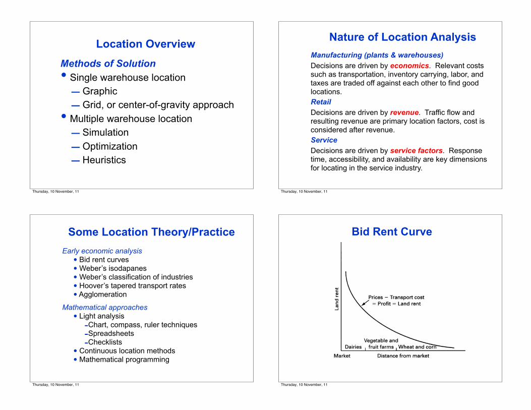
Methods of Solution• Single warehouse location
– Graphic– Grid, or center-of-gravity approach
• Multiple warehouse location– Simulation– Optimization– Heuristics
Location Overview
Thursday, 10 November, 11
Nature of Location AnalysisManufacturing (plants & warehouses)Decisions are driven by economics. Relevant costs such as transportation, inventory carrying, labor, and taxes are traded off against each other to find good locations.RetailDecisions are driven by revenue. Traffic flow and resulting revenue are primary location factors, cost is considered after revenue.ServiceDecisions are driven by service factors. Response time, accessibility, and availability are key dimensions for locating in the service industry.
Thursday, 10 November, 11
Some Location Theory/PracticeEarly economic analysis
• Bid rent curves• Weber’s isodapanes• Weber’s classification of industries• Hoover’s tapered transport rates• Agglomeration
Mathematical approaches• Light analysis
-Chart, compass, ruler techniques-Spreadsheets-Checklists
• Continuous location methods• Mathematical programming
Thursday, 10 November, 11
Bid Rent Curve
Thursday, 10 November, 11

Weber’s Classification of Industries
Thursday, 10 November, 11
Hoover’s Transport Curves
Thursday, 10 November, 11
CR (2004) Prentice Hall, Inc.
Method appraisal• A continuous location method• Locates on the basis of transportation costs alone
The COG method involves• Determining the volumes by source and destination point• Determining the transportation costs based on $/unit/mi.• Overlaying a grid to determine the coordinates of source and/or destination points• Finding the weighted center of gravity for the graph
COG Method
Thursday, 10 November, 11
COG Method (Cont’d)
where Vi = volume fluindo do e/ou para o ponto i Ri = custo unitário do transporte de Vi para o ponto iXi,Yi = coordenadas do ponto i = coordenadas do ponto a ser localizado
Thursday, 10 November, 11

COG Method (Cont’d)Example Suppose a regional medical warehouse is to be established to serve several Veterans Administration hospitals throughout the country. The supplies originate at S1 and S2 and are destined for hospitals at H1 through H4. The relative locations are shown on the map grid. Other data are: Note rate is a
per mile costPointi
Prod-ucts Location
Annualvolume,
cwt.
Rate,$/cwt/
mi. Xi Yi1 S1 A Seattle 8,000 0.02 0.6 7.32 S2 B Atlanta 10,000 0.02 8.6 3.03 H1 A & B Los
Angeles5,000 0.05 2.0 3.0
4 H2 A & B Dallas 3,000 0.05 5.5 2.45 H3 A & B Chicago 4,000 0.05 7.9 5.56 H4 A & B New York 6,000 0.05 10.6 5.2
Thursday, 10 November, 11
COG Method (Cont’d)Map scaling factor, K
Thursday, 10 November, 11
COG Method (Cont’d)
Solve the COG equations in table form
i Xi Yi Vi Ri ViRi ViRiXi ViRiYi1 0.6 7.3 8,000 0.02 160 96 1,1682 8.6 3.0 10,000 0.02 200 1,720 6003 2.0 3.0 5,000 0.05 250 500 7504 5.5 2.4 3,000 0.05 150 825 3605 7.9 5.5 4,000 0.05 200 1,580 1,1006 10.6 5.2 6,000 0.05 300 3,180 1,560
1,260 7,901 5,538
Thursday, 10 November, 11
COG Method (Cont’d)Now,
X = 7,901/1,260 = 6.27
Y = 5,538/1,260 = 4.40
This is approximately Columbia, MO.
The total cost for this location is found by:
where K is the map scaling factor to convertcoordinates into miles.CR (2004) Prentice Hall, Inc.
Thursday, 10 November, 11
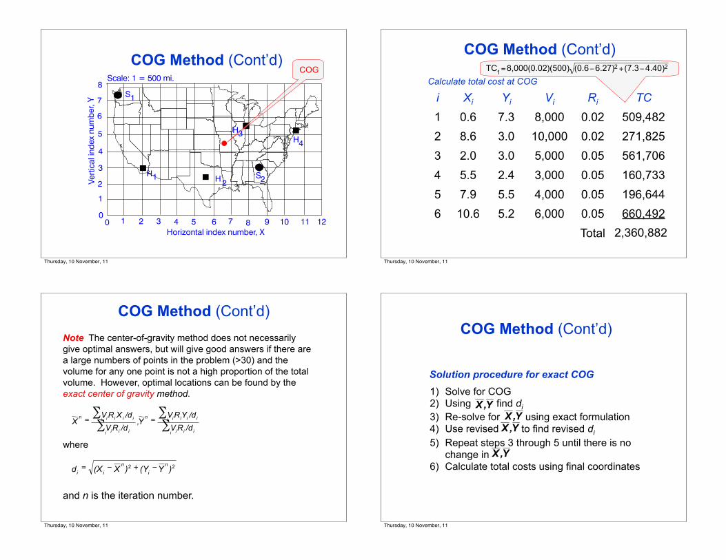
COGCOG Method (Cont’d)
Thursday, 10 November, 11
COG Method (Cont’d)
2,360,882Total660,4920.056,0005.210.66196,6440.054,0005.57.95160,7330.053,0002.45.54561,7060.055,0003.02.03271,8250.0210,0003.08.62509,4820.028,0007.30.61
TCRiViYiXiiCalculate total cost at COG
Thursday, 10 November, 11
Note The center-of-gravity method does not necessarilygive optimal answers, but will give good answers if there area large numbers of points in the problem (>30) and thevolume for any one point is not a high proportion of the totalvolume. However, optimal locations can be found by theexact center of gravity method.
∑∑
∑∑
==
i iii
i iiiin
i iii
i iiiin
/dRV/dYRV
Y,/dRV/dXRV
X
where
22 )Y(Y)X(Xdn
in
ii−+−=
and n is the iteration number.
COG Method (Cont’d)
Thursday, 10 November, 11
Solution procedure for exact COG
COG Method (Cont’d)
1) Solve for COG2) Using find di3) Re-solve for using exact formulation4) Use revised to find revised di
5) Repeat steps 3 through 5 until there is no change in
6) Calculate total costs using final coordinates
Thursday, 10 November, 11

CR (2004) Prentice Hall, Inc.
• A more complex problem that most firms have. • It involves trading off the following costs:
− Transportation inbound to and outbound from the facilities − Storage and handling costs− Inventory carrying costs− Production/purchase costs− Facility fixed costs
• Subject to:− Customer service constraints− Facility capacity restrictions
• Mathematical methods are popular for this type of problemthat:− Search for the best combination of facilities to minimize
costs− Do so within a reasonable computational time− Do not require enormous amounts of data for the analysis
Multiple Location Methods
Thursday, 10 November, 11
Location Cost Trade-Offs
Number of warehouses
Cos
t
Production/purchaseand order processing
Inventory carryingand warehousing
Warehousefixed
Inbound andoutboundtransportation
Total cost
00
CR (2004) Prentice Hall, Inc.
Thursday, 10 November, 11
CR (2004) Prentice Hall, Inc.
• A method used commercially- Has good problem scope- Can be implemented on a PC- Running times may be long and memory requirements substantial- Handles fixed costs well- Nonlinear inventory costs are not well
handled
• A linear programming-like solution procedure can be used (MIPROG in LOGWARE)
Mixed Integer Programming
Thursday, 10 November, 11
• Less complicated than previous example, butbased on integer programming
• Locates on basis of transportation costs andfacility fixed costs
• Locations are restricted to the node (e.g.,demand) points in the problem
• Method finds the optimal location of M facilities at a time
P-Median Location Method
Thursday, 10 November, 11

Example Five incinerators are to be located for toxic chemicalreclamation. The cost to move chemicals from 12 market areas tothe incinerators is $0.0867/cwt./mi. The areas, the chemicalvolume, and fixed costs to operate an incinerator are:
Market
Annualvolume,
cwt.
Fixedoperating
cost, $ Market
Annualvolume,
cwt.
Fixedoperating
cost, $Boston MA 30,000 3,100,000 Chicago IL 240,000 2,900,000New York NY 50,000 3,700,000 Minneapolis MN 140,000 --Atlanta GA 170,000 1,400,000 Phoenix AZ 230,000 1,100,000Baltimore MD 120,000 -- Denver CO 300,000 1,500,000Cincinnati OH 100,000 1,700,000 Los Angeles CA 40,000 2,500,000Memphis TN 90,000 -- Seattle WA 20,000 1,250,000
P-Median (Cont’d)
13-31
Thursday, 10 November, 11
The database for this problem is PMED02.DAT inLOGWARE.
AnswerNo. Facility name Volume Assigned
node numbers 1 New York NY 200,000 1 2 4 2 Atlanta GA 260,000 3 6 3 Chicago IL 480,000 5 7 8 4 Phoenix AZ 270,000 9 11 5 Denver CO 320,000 10 12 Total 1,530,000
Total cost: $24,739,040.00and graphically shown…
P-Median (Cont’d)
Thursday, 10 November, 11
P-Median (Cont’d)
Repeating the analysis for a different number of incinerators can find the optimal number of incinerators as well.
13-33
Thursday, 10 November, 11
Selective Evaluation Using COG
Note : Inventorycosts and fixedcosts increase withmore warehouses
User selects the locations or the number of locations to be evaluated. Analysis is repeateduntil the optimum is found. Inventory value can be easily added as in the following examplewhere I NT = $6, ,000 000 . At 25% per year, the inventory carrying cost is CC = 0.25 I T .
Number ofWarehouses
TransportationCost, $
FixedCost, $
InventoryCost, $
TotalCost, $
1 41,409,628 2,000,000 1,500,000 44,909,6282 25,989,764 4,000,000 2,121,320 32,111,0843 16,586,090 6,000,000 2,598,076 25,184,1664 11,368,330 8,000,000 3,000,000 22,368,3305 9,418,329 10,000,000 3,354,102 22,772,4316 8,032,399 12,000,000 3,674,235 23,706,6347 7,478,425 14,000,000 3,968,627 25,447,0528 2,260,661 16,000,000 4,242,641 22,503,3029 948,686 18,000,000 4,500,000 23,448,686
10 0 20,000,000 4,743,416 24,743,416
Note : Transport cost declinewith more warehouses
Example
13-34
Thursday, 10 November, 11

Shows effect of inventory policy on location. Presence of local optima make it difficult to find the optimum solution in complex problems.
Total Cost Curve for Selective Evaluation Example
0
12,500,000
25,000,000
37,500,000
50,000,000
Total cost, $
1 2 3 4 5 6 7 8 9 10
Number of warehouses
Local optimumOptimum
Thursday, 10 November, 11
Location by Simulation
CR (2004) Prentice Hall, Inc.
•Can include more variables than typical algorithmic methods
•Cost representations can be precise so problem can be more accurately described than with most algorithmic methods
•Mathematical optimization usually is not guaranteed, although heuristics can be included to guide solution process toward satisfactory solutions
•Data requirements can be extensive
•Has limited use in practice
Thursday, 10 November, 11
Shyc
on/M
affe
i Sim
ulat
ion
CR (2004) Prentice Hall, Inc.
Thursday, 10 November, 11
Commercial Models for Location
Features
•Includes most relevant location costs
•Constrains to specified capacity and customer service levels
•Replicates the cost of specified designs
•Handles multiple locations over multiple echelons
•Handles multiple product categories
•Searches for the best network design
CR (2004) Prentice Hall, Inc.
Thursday, 10 November, 11
CR (2004) Prentice Hall, Inc.
Com
mer
cial
Mod
els
(Con
t’d)
13-45
Thursday, 10 November, 11
CR (2004) Prentice Hall, Inc.
Commercial Models (Cont’d)
13-46
Thursday, 10 November, 11
CR (2004) Prentice Hall, Inc.
Dynamic Location
Retail Location
Methods
• The general long-range nature of the location problem- Network configurations are not implemented immediately- There are fixed charges associated with moving to a new
configuration
• We seek to find a set of network configurations that minimizes the presentvalue over the planning horizon
• Contrasts with plant and warehouse location.- Revenue rather than cost driven- Factors other than costs such as parking, nearness to competitive
outlets, and nearness to customers are dominant
• Weighted checklist - Good where many subjective factors are involved - Quantifies the comparison among alternate locations
Thursday, 10 November, 11
CR (2004) Prentice Hall, Inc.
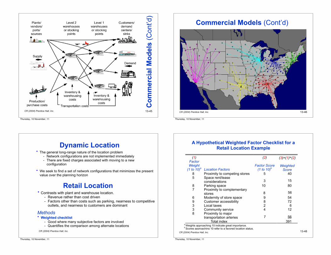
A Hypothetical Weighted Factor Checklist for a Retail Location Example
(1)FactorWeight
(1 to 10)a Location Factors
(2)
Factor Score(1 to 10)b
(3)=(1)×(2)
WeightedScore
8 Proximity to competing stores 5 405 Space rent/lease
considerations 3 158 Parking space 10 807 Proximity to complementary
stores 8 566 Modernity of store space 9 549 Customer accessibility 8 723 Local taxes 2 63 Community service 4 128 Proximity to major
transportation arteries 7 56 Total index 391
13-48
Thursday, 10 November, 11
Top Related