


Languages
Pages
Legal


EXPLORATORY MULTIVARIATE STATISTICAL METHODS APPLIED TO PHARMACEUTICAL
INDUSTRY CRM DATA
by
Jorge Manuel Santos Freire Tavares
Dissertation submitted in partial fulfilment of the requirements for the degree of
Mestre em Estatística e Gestão de Informação
[Master of Statistics and Information Management]
Instituto Superior de Estatística e Gestão de Informação
da
Universidade Nova de Lisboa

II
EXPLORATORY MULTIVARIATE STATISTICAL METHODS APPLIED TO PHARMACEUTICAL
INDUSTRY CRM DATA
Dissertation supervised by
Professor Doutor Fernando Lucas Bação
Professor Doutor Pedro Simões Coelho
November 2007

III
Acknowledgements To Professor Fernando Lucas Bação and Professor Pedro Simões Coelho for their orientation
and support during the execution of this work.
To my friends and family, because of my needed absences to do this work, thank you very much
for the support and understanding.

IV
ABSTRACT
An analysis of the current CRM systems in the Pharmaceutical Industry, the way the
pharmaceutical companies developed them and a comparison between Europe and United States
was done in this study. Overall the CRM in the pharmaceutical industry is far-behind, when
compared with other business areas, like consumer goods, finance (banking) or insurance
companies, being pharmaceutical CRM specifically less developed in Europe when compared to
United States.
One of the big obstacles for the success of CRM in the pharmaceutical industry is the poor
analytics applied to the current CRM programs. Improving Sales and Marketing Effectiveness
by apllying, multivariate exploratory statistical methods, specifically Factor Analysis and
Clustering into pharmaceutical CRM data from a Portuguese pharmaceutical company was the
main goal of this thesis. Their overall usefulness when applied to the business was
demonstrated, and specifically in relation to the cluster methods, SOMs outperformed the
hierarchical methods by producing a more meaningful business solution.
RESUMO Neste estudo, foi feita uma análise dos sistemas de CRM actualmente utilizados na indústria
farmacêutica, a maneira como as empresas farmacêuticas os desenvolvem, fazendo uma
comparação entre a Europa e os Estados Unidos da América. Na sua globalidade o CRM na
indústria farmacêutica está menos desenvolvido quando comparado com outras áreas de
negócio, tais como o grande consumo, banca ou seguradoras, sendo ainda menos desenvolvido
o CRM farmacêutico na Europa quando comparado com os Estados Unidos.
Um dos grandes obstáculos para o sucesso do CRM na indústria farmacêutica é a fraca análise
de dados feita nos actuais programas de CRM. Melhorar a eficiência nos processos associados
ao marketing e ás vendas, usando métodos exploratórios de análise multivariada,
especificamente Análise Factorial e Análise de Clusters, aplicados a um conjunto de dados
proveniente de uma empresa farmacêutica Portuguesa, é o principal objectivo desta tese. A
utilidade destes métodos quando aplicados no contexto da área de negócio em estudo
demonstrou a sua utilidade e especificamente em relação á análise de clusters, globalmente os
métodos hierárquicos foram inferiores na produção de uma solução válida para a área de
negócio em questão quando comparados com os SOMs.

V
Key Words
Customer Relatationship Management
Pharmaceutical Industry
Exploratory Multivariate Statistical Methods
Factor Analysis
Hierarchical Cluster analysis
Self- Organizing Map
Palavras- Chave.
Gestão de Relacionamento do Cliente
Indústria Farmacêutica
Analise de Dados Exploratória Multivariada
Análise Factorial
Análise Hierárquica de Clusters
Mapa Auto Organizável de Kohonen.

VI
Abbreviations
BMU Best Matching Unit
CLTV Customer Life Time Value
CRM Customer Relationship Management
DTC Direct to Consumer Advertising
ERP Enterprise Resourse Planing
HMO Health Maintainance Organization
IMS International Marketing Services
PAF Principal Axis Factoring
PCF Principal Components Factoring
PhRMA Pharmaceutical Research and Manufacturers of America
qe Average quantization error
SFA Sales Force Automation
SOM Self- Organizing Map
te Topographic error
U-Matrix Unified Matrix
U.S. United States

VII
Table of contents 1. INTRODUCTION..................................................................................................................... 1
1.1. Context............................................................................................................................... 1
1.2. Motivation.......................................................................................................................... 2
1.3. Objectives .......................................................................................................................... 3
1.4. Structure of the dissertation ............................................................................................... 4
2. LITERATURE ANALYSIS................................................................................................. 5
2.1. CURRENT PHARMACEUTICAL ENVIRONMENT..................................................... 7
2.1.1 Characteristics of the United States of America Pharmaceutical Market.................... 7
2.1.2 Characteristics of the European Pharmaceutical Market............................................. 7
2.1.3 Direct-To-Consumer advertising United States of America versus Europe and the
changing dynamics of promoting pharmaceutical drugs ...................................................... 8
2.2. ANALYSIS OF THE CURRENT CRM PROGRAMS IN THE PHARMACEUTICAL
INDUSTRY. ........................................................................................................................... 11
2.2.1 General Overview of CRM Programs in the Pharmaceutical Industry ..................... 11
2.2.2 Sales Force Automation Systems in Pharmaceutical Industry .................................. 14
2.2.3 CRM Programs focusing in online strategies and communication technologies ...... 19
2.2.4 CRM focusing in Supply Chain and Demand Management Integration ................... 22
2.2.5 Differences between the current CRM programs in Europe and United States ........ 23
3. METHODOLOGY.................................................................................................................. 25
3.1 BUSINESS PURPOSE OF APPLIYING MULTIVARIATE TECHNIQUES IN
PHARMACEUTICAL CRM.................................................................................................. 25
3.2 DESCRIPTION OF THE CRM DATA FILE USED. ...................................................... 26
3.3 FACTOR ANALYSIS ...................................................................................................... 28
3.3.1 Factor Model ............................................................................................................. 28
3.3.2 Factor Indeterminacy................................................................................................. 30
3.3.3 Factor Rotations......................................................................................................... 31
3.3.4 Data Matrix................................................................................................................ 37
3.3.5 Factor Extraction Methods ........................................................................................ 37
3.3.6 Methods to evaluate if data is appropriate for factor analysis ................................... 40
3.3.7 Determining the number of factors............................................................................ 41
3.3.8 Factor Solution Quality ............................................................................................. 44
3.3.9 Factor Scores ............................................................................................................. 45
3.3.10 Factor Analysis versus Principal Components Analysis ......................................... 46
3.3.11 Exploratory versus Confirmatory Factor Analysis .................................................. 47
3.4 HIERARCHICAL CLUSTERING................................................................................... 48

VIII
3.4.1 Introduction ............................................................................................................... 48
3.4.2 Agglomerative Methods ............................................................................................ 48
3.4.3 Distance Measures..................................................................................................... 51
3.4.4 Techniques to decide the number of Clusters............................................................ 56
3.4.5 Assess Reliability and Validity.................................................................................. 58
3.5 SELF-ORGANIZING MAPS........................................................................................... 61
3.5.1 Introduction ............................................................................................................... 61
3.5.2 Basic SOM Learning Algorithm: .............................................................................. 63
3.5.3 Neighbourhood Functions ......................................................................................... 63
3.5.4 U- Matrix ................................................................................................................... 64
3.5.5 Component Planes ..................................................................................................... 65
3.5.6 SOM Quality ............................................................................................................. 65
3.5.7 Market Segmentation using Self- Organizing Maps ................................................. 66
3.5.8 SOM Implementation in MATLAB .......................................................................... 67
4. RESULTS ............................................................................................................................... 70
4.1. DESCRIPTIVE REPORTING......................................................................................... 70
4.2. CHARACTERIZATION OF THE RELATIONSHIP BETWEEN BUSINESS
ATTRIBUTES. ....................................................................................................................... 75
4.3 CUSTOMER SEGMENTATION..................................................................................... 91
5. CONCLUSIONS AND FUTURE DEVELOPMENTS ........................................................ 110
6. REFERENCES...................................................................................................................... 115
APPENDIX A ........................................................................................................................... 118
APPENDIX B ........................................................................................................................... 131
APPENDIX C ........................................................................................................................... 138
APPENDIX D ........................................................................................................................... 158

IX
List of tables Table 1- Overview of the regional market differences between Europe and United States (CGEY &
Young and INSEAD 2002) ................................................................................................................10 Table 2- CRM dataset variables measured in 2004. ................................................................................27 Table 3- KMO measure of appropriateness for factor analysis .............................................................41 Table 4- Crosstabs with the values used for the association measures..................................................52 Table 5- SOM parameters in SOM toolbox in MATLAB (Vesanto et al. 2000) ..................................67 Table 6- Descriptive statistics per variable per region............................................................................71 Table 7- Correlation Matrix of the variables in analysis ........................................................................74 Table 8- Factor Analysis KMO and Bartlett’s Test for all the observations........................................76 Table 9- Factor Analysis KMO and Bartlett’s Test excluding outliers.................................................76 Table 10- PCF Factor Analysis Anti- image Matrices for all the observations....................................77 Table 11 - PCF Factor Analysis Anti- image Matrices for all the observations...................................77 Table 12 - Factor analysis Communalities for PCF two factors extraction method............................79 Table 13- PCF Factor Analysis Eigenvalues for two factor extraction .................................................79 Table 14- PCF Factor Matrix for two factor extraction .........................................................................80 Table 15- PCF Varimax Rotation Factor Matrix- two factor extraction..............................................81 Table 16- PCF Reproduced and Residual Correlation Matrices for two factors extraction..............81 Table 17- Factor analysis Communalities for PCF three factors extraction method..........................82 Table 18- PCF Factor Analysis Eigenvalues for three factor extraction ..............................................82 Table 19- PCF Factor Matrix for three factor extraction.......................................................................83 Table 20- PCF Varimax Rotation Factor Matrix for three factor extraction .....................................83 Table 21-PCF Reproduced and Residual Correlation Matrices for three factors extraction ............84 Table 22- Factor analysis Communalities for PAF two factors extraction method.............................85 Table 23- Factor analysis Communalities for PAF two factors extraction method.............................85 Table 24- PAF Factor Matrix for two factor extraction .........................................................................85 Table 25-PAF Varimax Rotation Factor Matrix- two factor extraction...............................................86 Table 26-PAF Reproduced and Residual Correlation Matrices for two factors extraction...............86 Table 27- Factor analysis Communalities for PAF two factors extraction method.............................87 Table 28- PAF Factor Analysis Eigenvalues for three factor extraction ..............................................87 Table 29- PAF Factor Matrix for three factor extraction.......................................................................87 Table 30- PAF Varimax Rotation Factor Matrix for three factor extraction ......................................88 Table 31- PAF Reproduced and Residual Correlation Matrices for three factors extraction ...........88 Table 32- RMSR calculated for the different methods. ..........................................................................89 Table 33- Factor labels and comments......................................................................................................89 Table 34- Dendogram solutions for the entire data set using the five clustering methods .................92 Table 35- Values for the last cluster solutions using the Mojena criteria .............................................93 Table 36- Custer solutions obtained according to the selection technique and the clustering method
..............................................................................................................................................................93 Table 37- Cluster solutions using the different clustering methods.......................................................94 Table 38- Characteristics of the top 6 hospitals .......................................................................................94 Table 39- Cophenetic Correlation Coeficients for the 5 different clustering methods........................95 Table 40- Dendogram solutions for the data set without outliers using the five clustering methods 96 Table 41- Values for the last cluster solutions without outliers using the Mojena criteria.................97 Table 42- Custer solutions obtained according to the selection technique and the clustering method
used excluding the outliers ................................................................................................................98 Table 43- Cluster solutions using the different clustering methods without using the outliers .........98 Table 44- Dashboard for the 5 cluster solution with ward method including all observations..........99 Table 45- Dashboard for the 5 cluster solution with ward method excluding the outliers ...............100 Table 46- Dashboard for the 5 cluster solution with ward method excluding the outliers ...............101 Table 47- Average quantization (qe) and topological errors (te) obtained.........................................105 Table 48- Dashboard with the SOM clustering solution .......................................................................106 Table 49- Dashboard with the SOM clustering solution with churners..............................................107 Table 50- Differences between the hierarchical methods and SOM in terms of the results achieved
............................................................................................................................................................108

X
List of figures Figure 1-The changing network of prescribing influence makers...........................................................9 Figure 2- Traditional push promotional channels in Pharmaceutical Industry ..................................14 Figure 3- Projection of vectors onto a two-dimentional space in a orthogonal factor model .............32 Figure 4- Oblique factor model-pattern loading......................................................................................36 Figure 5- Oblique factor model- structure loading..................................................................................36 Figure 6- Oblique factor model-pattern and structure loadings............................................................37 Figure 7- Cattell's scree test example ........................................................................................................42 Figure 8- Linkage methods; (a) single linkage; (b) complete linkage; average linkage adapted from
(Branco 2004)......................................................................................................................................49 Figure 9- Dendogram for hypothetical data .............................................................................................56 Figure 10- U-matrix .....................................................................................................................................65 Figure 11- Component planes.....................................................................................................................65 Figure 12- Map lattice and discrete neighbourhoods of the centremost unit. a) hexagonal lattice, b)
rectangular lattice. The innermost polygon corresponds to 0 neighbourhood, the second to 1 neighbourhood and the biggest to 2 neighbourhood. Adapted from (Vesanto et al. 2000)......68
Figure 13- Example of training of a SOM in a 2D input space. Note that the initial positions (in black) of the BMU and its neighbouring units are updated (in grey) according to the data patter (cross) presented to the SOM. Adapted from (Vesanto et al. 2000) .................................68
Figure 14- Activity performance................................................................................................................72 Figure 15- Z-Scores per variable per customer........................................................................................73 Figure 16- Factor analysis scree plot .........................................................................................................78 Figure 17- Factor analysis Parallel analysis .............................................................................................78 Figure 18-Agglomeration coefficient graphs for the 5 clustering methods...........................................92 Figure 19- Agglomeration coefficient graphs for the 5 clustering methods without outliers .............97 Figure 20- Component planes for the original variables.......................................................................103 Figure 21- U-matrix with neurons labelled.............................................................................................104 Figure 22- U-matrix with the hits and clusters pointed out. Small distances are represented at blue
while large are at red .......................................................................................................................104 Figure 23- SOM component planes .........................................................................................................105 Figure 24- ACE Concept for enhancement of the current CRM-SFA programs..............................114

1
1. INTRODUCTION ______________________________________________________________________
1.1. Context IMS, the world biggest supplier of pharmaceutical drug sales information, estimates that the
total value of the pharmaceutical market reached more than 560 thousand of millions US dollars
in 2006 (IMS 2007), making the pharmaceutical industry one of the most important businesses
in the world.
There are two types of medicines, the ethical drugs (prescribed by the physician) and the over
the counter drugs (OTCs) that are sold without the need of a medical prescription. In the OTCs,
the pharmaceutical industry can advertise directly to the patient, in the case of the ethical drugs,
only the healthcare professionals can receive promotion and scientific information in the
European Union.
In the USA it is possible to promote the ethical drugs directly to the patient, but like in Europe,
these drugs are prescribed by the physician, and for that reason the physician is the main target
of the pharmaceutical companies. The OTCs represent less than 10% of the total global market,
being the ethical drugs the main slice of the market. The ethical drugs can be divided in drugs
that are sold in Retail Pharmacies or in Hospitals.
With very restricted rules of advertising and promotion, and with the power of decision, mainly
centralized in the physicians, the pharmaceutical industry never developed advanced models of
market analysis (Carpenter 2006), like the other markets (ex: mass market, banking, insurance
companies, automobile industry, telecommunications, etc).
Nevertheless times are changing, patients have more access to information mainly trough
internet, and also with the cost containment measures that many European countries are
applying, including Portugal, the physicians are no longer the sole decision makers in the
process of prescription. The health authorities are pushing the generics into the market,
advertising them to the consumers, and allowing the pharmacists to replace under certain
conditions a brand ethical drug for a generic. In Hospitals the board of directors are also pushing
the physicians to use the most cost-effective drugs. So basically in the past, the pharmaceutical
industry relied in the quality of their drugs and in the ability of the sales reps to promote it to the
2
physicians, to achieve their sales goals. Now with the new stakeholders both in the retail and
hospital market, the reality is becoming more complex to be managed by the pharmaceutical
companies.
This thesis will focus in Customer Relationship Management in Pharmaceutical Industry.
Usually when looking to the Market, the pharmaceutical companies divide their clients in three
different types:
1. The hospitals or other institutions that buy pharmaceutical drugs.
2. The health professionals.
3. The patients (mainly in the USA).
The Pharmaceutical companies, very often segment the Hospitals using bivariate matrix’s (like
ABC type matrix), and the health professionals in targeted professionals and non-targeted
professionals. The target professionals are also usually ranked (ex: ABC) by prescribing or
influence to prescribe importance of a certain drug (Lerer and Piper 2003). Other external
influencers are gaining growing importance such as the Health Authorities or any other private
insurance institution (particularly in the United States) that are responsible for the
reimbursement of drugs, because very often it is required their approval before a drug can enter
in the market (Datamonitor 2006).
1.2. Motivation
The reason for the choice of the thesis topic, it is related to the fact that is starting to be an
important debate in the pharmaceutical industry, the need to have more sophisticated analysis
that can increase the efficiency of both marketing strategies and sales force activity in the field.
It was one of the main topics of the last European Sales Force Effectiveness Summit that took
place in Barcelona during March 2006.
Many pharmaceutical companies invested large amount of money in implementing Customer
Relationship Management (CRM) Tools. These systems should help pharmaceutical companies
to deal with the increase complexity of the market, providing segmentations of their clients
based on their customer profiles, but research from international analysts suggests that, across
all pharmaceutical industries, as much as 80 per cent of current CRM programmes will fail to
deliver satisfactory returns for the companies that have bough into them (Carpenter 2006). We
can easily conclude that there is a lot to be done in terms of CRM and market analysis in the
pharmaceutical industry.

3
Most of the European pharmaceutical companies are using their CRM systems as Sales Force
Automation Tools (SFA) producing basic reports, using only descriptive statistics (Carpenter
2006; Lerer and Piper 2003). Still in the Pharmaceutical Industry the product focus strategy is
predominant versus the customer centric approach (Lerer and Piper 2003). Is still common in
the pharmaceutical industry to have sales forces promoting only one product, but considering
that the estimated average cost of a sales representative visit to a physician in Europe is 150
Euros (Lerer and Piper 2003), and with the strong cost-containment governmental measures in
Europe concerning pharmaceutical drugs, the high margins in the pharmaceutical industry are
going down, so that approach will not be feasible in the future (Lerer and Piper 2003). Currently
the pharmaceutical industries are trying to find ways to save money and improve their
operational effectiveness in order to try to protect their margins. CRM in the pharmaceutical
industry should help pharmaceutical industry to improve their sales and marketing effectiveness
by accessing and enabling synergies between the existing drugs in the promotional effort (factor
analysis technique could be used for this purpose), and by developing customer segmentations
(using clustering techniques) that use all the critical business variables to segment the customers
not only by their value (current standard in pharmaceutical industry) but also by their specific
characteristics. A dataset from a CRM system from a Pharmaceutical Company operating in the
Portuguese hospital market is available to conduct the analysis mentioned above. The lack of
studies using multivariate statistical techniques in pharmaceutical CRM, when simple
descriptive statistics seem to be insufficient to provide the best business direction in a market
that must study more deeply the combined interaction of the business attributes to get a higher
sales and marketing efficiency is also an extra motivation for this thesis.
1.3. Objectives
The aim of this study is:
1. Do an analysis of the current CRM systems in the Pharmaceutical Industry, the way the
pharmaceutical companies developed them, and make a comparison between Europe
and United States.
2 Evaluate if exists or not relationships between the different business attributes (related
to the pharmaceutical business) in order to improve sales and marketing effectiveness of
the company by evaluating synergies and patterns established between the products and
the other business attributes in order to give strategic marketing insights and also to
promote the correct deployment of sales forces.

4
3 Provide customer segmentation that promotes synergies between business attributes and
enables alignment between sales and marketing strategies.
It will be our aim to find relationships between the business variables in the company CRM
dataset (product sales per hospital; sales representatives activities per hospital; number of
chemotherapy patients treated per hospital) in order to give evidence to the marketing
department which variables correlate together and can help driving the sales of the different
products, and also to deploy multi-product sales force that will promote products that share
common business characteristics, factor analysis will be used to help achieving these objectives.
Secondly we will segment company customers (Hospitals) not only by value but also by their
overall characteristics by using multivariate clustering techniques. Our analysis focus in the
European perspective of CRM, where CRM strategies where mainly developed around SFA
tools, with a specific focus in the Oncology Portuguese Hospital Market.
1.4. Structure of the dissertation
The structure of the dissertation is organized as follows. The introduction (Chapter 1) presents
the context, the goals and the purpose of the study and summarizes the structure of the
dissertation.
In Chapter 2 an analysis of the pharmaceutical market with an emphasis in United States and
Europe, together with a detailed analysis of the Customer Relationship Management in the
pharmaceutical industry, making a comparison between Europe and United States, is done.
In Chapter 3, the business purpose of applying multivariate techniques in pharmaceutical CRM
is described together with the description of the dataset used in our thesis. Also theoretical
concepts of exploratory multivariate techniques, specifically Factor Analysis and Clustering
techniques are described.
In Chapter 4, Factor Analysis and Clustering techniques are applied to real pharmaceutical
CRM data and the results and findings are discussed. The multivariate statistical techniques are
used according with the business needs and a comparison of hierarchical clustering methods
with Self-Organizing Maps is performed. In this chapter is also shown how the type of data used
can influence the decisions regarding the different multivariate statistical methods applied.
Chapter 5, presents the conclusions, some limitations of this work and future developments.

5
2. LITERATURE ANALYSIS ______________________________________________________________________ The total value of the pharmaceutical market reached more than 560 thousand of millions US
dollars in 2006 (IMS 2007), making the pharmaceutical industry one of the most important
businesses in the world.
Being a business area with a large financial capacity, many pharmaceutical companies invested
large amount of money in implementing Customer Relationship Management (CRM) Tools.
These systems should help pharmaceutical companies to deal with the increase complexity of
the market, providing segmentations of their clients based on their customer profiles, but in fact
most of the CRM programs implemented failed to deliver satisfactory returns for the companies
that have bough into them (Carpenter 2006). It is rumoured that one major pharmaceutical
company spent 200 million dollars on a CRM system that was never launched because it failed
to meet expectations (Lerer and Piper 2003).
Although other methods are also used to promote drugs, notably events, symposia and medical
journal advertising, sales force detailing remains the dominant approach, consuming over 70 per
cent of marketing budgets, so it was expected that the CRM programs could help
pharmaceutical companies to gain efficiencies in the sales force in order to reduce costs in an
area with a big impact in the overall pharmaceutical companies budgets, but weak analytics
applied to CRM-SFA systems did not enabled their correct usage neither to gain efficiency or to
improve customer segmentation (Lerer and Piper 2003).
One of the big issues in the pharmaceutical marketing it is the product focus approach that it is
still dominant versus the customer centric approach that it is critical for the successes of a CRM
program. Together with the excessive product focus approach it is the use of basic and poor
segmentations (bivariate segmentations) that are an obstacle to the pharmaceutical companies
knowledge of their customers. Others industries, like for example consumer goods use tools, to
collect information about the consumers and use more complex analysis to get a deeper
understanding about their needs (Lerer 2002). Pharmaceutical industry should adapt the best
practices of other areas to their own business (Lerer and Piper 2003).

6
Understanding customer’s needs is essential to maintain their loyalty and also to increase their
value by giving them the products or services that will satisfy them (Kotler and Keller 2007).
Pharmaceutical companies should maximize the synergies between the products in their
portfolio (Lerer and Piper 2003).
Currently a good customer segmentation should identify not only the high value customers but
segment them by their characteristics (Pepers and Rogers 2006), identify the midsize customers,
because usually they demand good service in a reasonable way, pay nearly full price, and are
often the most profitable and identify the low value customers, specifically the ones that the
company should not invest promotional effort (Kotler and Keller 2007). In the current hospital
market that is the source of our pharmaceutical company dataset, pharmaceutical companies are
facing tender negotiations per hospital resulting from the current governmental cost-
containment pressures what is changing the hospital market to a type of market similar to other
industries like the consumer goods (Garrat 2006; Lerer and Piper 2003), and if the segmentation
above applies very well to the consumer goods industry it should also make sense to apply to
the pharmaceutical market.
The pharmaceutical market is a highly regulated area where two big markets have a dominant
position in the world, the European and the United States markets. The way the pharmaceutical
market is structured the current changes in the pharmaceutical market, and the differences
between the European and the United States markets are subject to further analysis ahead in the
literature review. Subsequently to the analysis of the pharmaceutical environment, an analysis of
the current CRM programs is done and the differences between the current CRM programs in
Europe and United States are also analysed taking in consideration how the differences between
the two markets could have influenced the development of the CRM programs. Overall the
literature review plays a key role in this thesis and it will be fundamental to accomplish the first
objective of our study mentioned in the previous section.

7
2.1. CURRENT PHARMACEUTICAL ENVIRONMENT ______________________________________________________________________
2.1.1 Characteristics of the United States of America Pharmaceutical Market
In 2006, the North American market (United States and Canada, but with more than 93 per cent
of the sales coming from USA) was dominating, representing 47 percent of worldwide drug
revenues (266 thousand of millions dollars), followed by Europe with 30 percent and Japan with
11 percent (IMS 2007). American pharmaceutical companies focus on core competencies and
are today called “life science companies”. Supported by high revenues, they are leaders in the
development and commercialization of innovative therapy approaches. The relative position of
the United States as a place of innovation has increased over the past decade. During the past
few decades, investment in R&D has continued to grow in the United States. Accompanying
this increased investment is a doubling of the number of drugs in clinical or later development,
from more than 1300 in 1997 to more than 2700 in 2005. In the United States the drug pipeline
growth contrasts with trends in Europe, where rigid government policies have discouraged
continued pharmaceutical discovery (PhRMA 2006).
Price competition is very strong in this liberal environment. However, due to pressure applied
by the Health Maintenance Organizations (HMOs) Pharmaceutical Benefit Managers (PMB) on
the reduction of drug prices, prices have remained fairly stable since the mid-1990s (Schulman
et al 1996). The U.S. pharmaceutical market is characterized by an uptake of new products
relying on price premium and marketing access; generics and therapeutic substitution (the use of
generics by physicians is encouraged by HMOs); an expansion of access and usage; and an
emerging parallel trade (Lerer and Piper 2003).
2.1.2 Characteristics of the European Pharmaceutical Market
Europe’s pharmaceutical market share represented 30 percent of the total world market in 2006
(IMS 2007), accounting for 169 thousand of millions dollars. Europe is composed of countries
with different health care systems, and different laws for controlling pharmaceutical production,
logistic, distribution and sales.
There are five big markets in Europe, Germany and France represent about half of the European
market together with Italy, Spain and the United Kingdom they represent 75 percent of the
European market (Redwood 2007).

8
There is an intensified cost-containment policy in Europe and the pharmaceutical industry is a
target for savings. This leads to an active encouragement of generics and restrictions in
reimbursement of new drugs. The medical drug prices differ due to the different approaches
used by the E.U. member states for regulating pharmaceutical prices. The cheapest medicines
are found in the poorer countries such as Portugal and Greece. The prices in the Netherlands,
Denmark, Ireland, the United Kingdom and Belgium are the highest (Garratt 2006; Lerer and
Piper 2003).
2.1.3 Direct-To-Consumer advertising United States of America versus Europe and the changing dynamics of promoting pharmaceutical drugs
Most probably the biggest difference between Europe and the United States in the area of
promoting drugs is the fact that the United States allows advertising of prescription drugs to the
public.
In the United States pharmaceutical companies have been aggressively targeting consumers
since 1997 when pharmaceutical advertising regulations were relaxed. Since then United States
pharmaceutical companies spent huge amounts of money in direct-to-consumer (DTC)
advertising, in the year 2000 an estimated 2300 million dollars was spent on DTC advertising
(Lerer and Piper 2003).
Contrary to some reports in 2001, the European Union maintained the ban on DTC advertising.
Instead, European Union commissioners debated a provision allowing pharmaceutical
companies to provide the patients with non promotional data about prescription drugs for
specific chronic diseases (Lerer and Piper 2003). For example in Portugal the pharmaceutical
industry is allowed to give drug information to a patient if requested specifically by the patient.
Both in Europe and United States, the sales reps are finding harder than ever to gain access to
physicians to detail drugs. Some countries like France and Portugal are also imposing
governmental measures to limit the access of sales reps (sales representatives) to physicians
(Datamonitor 2006). Because of these difficulties, pharmaceutical companies have been
exploiting new marketing channels to reach the health professionals like the Internet and the E-
Learning (Datamonitor 2006; Lerer and Piper 2003).
While physicians remain an important target for promoting activities the growing influence of
other stakeholders, such as nurses, pharmacists and patients is having impact on prescribing
choices. Also the Health Authorities or any other private insurance institutions (particularly in

9
the United States) that are responsible for the reimbursement of drugs are important targets for
the pharmaceutical companies (Datamonitor 2006).
Figure 1-The changing network of prescribing influence makers
The diagram above explains very well how the different stakeholders influence the prescription
process, and how their influence in the process is being changed by the current environment.
The physicians are currently losing influence in the process because the key purchasing groups
(hospitals, insurers, governments, HMOs), both in Europe and United States are tightening cost-
containment policies by using restricted formularies, encouraging generic substitution and
limiting reimbursement, limiting the options available for the physician to prescribe. In the
United States and United Kingdom is possible to other health professionals, like nurses and
pharmacists with complementary training to prescribe certain pharmaceutical drugs
(Datamonitor 2006), but specifically the pharmacists are growing their influence because many
European Governments are allowing direct substitution by a generic in a pharmacy by a
pharmacist when a brand drug loses patent and a generic is already available (Redwood 2007).
The patients influence as grown a lot in the last years, patients are now searching information
about the quality and safety of the pharmaceutical drugs and influencing the physicians in the
drugs they prescribe (Datamonitor 2006; Lerer and Piper 2003). One recent survey showed that
sales representatives and consumers have similar influencing powers on physicians prescribing
decisions both in United Sates and Europe (Datamonitor 2006). Another survey conducted in
the United States revealed that 71 per cent of patients who requested a specific drug were indeed
prescribed that product (Lerer and Piper 2003).
There is no doubt that informed patients are influencing physician prescribing, but also lobbing
to have access to the best drugs. The accelerated approval of Glivec, an innovative anti-cancer

10
treatment develop by the pharmaceutical company Novartis, can to a great extent be attributed
to the activism of leukaemia patients and their families, who demanded that the drug, after
showing near-spectacular efficacy in early clinical trails be made available without delay (Lerer
and Piper 2003). The fact that DTC advertising in Europe is not allowed does not stops
European patients to access Internet and get the same type of information that most of the
United Sates patients receive (Datamonitor 2006; Lerer and Piper 2003).
Table 1- Overview of the regional market differences between Europe and United States (CGEY & Young and INSEAD 2002)
The table above resumes most of what as been already mentioned in this study about the
characteristics of the United States and European Market. Nevertheless it is important to
emphasis that the physician’s time spent with sales reps, specially the high prescribers, is
saturated in the United Sates and near saturation in Europe, because both in Europe and United
States the pharmaceutical companies increased their sales force size every year in the last
decade. The sales forces in South Europe countries are usually bigger in size because the
physicians in Southern European countries are usually more available to interact more often
with the sales representatives from the pharmaceutical companies than their colleges from
Central and North Europe countries (Datamonitor 2006; Lerer and Piper 2003).
Another very important difference between United States and Europe is regarding prescribing
data availability, because in Europe in opposition to United States there are strong privacy laws
and the customer sales data is presented at aggregated level, stripped of personal identification
information. But even in United Sates, regulatory authorities are study some measures to control
the access to personal information (Datamonitor 2006; Lerer and Piper 2003).

11
2.2. ANALYSIS OF THE CURRENT CRM PROGRAMS IN THE PHARMACEUTICAL INDUSTRY.
______________________________________________________________________
2.2.1 General Overview of CRM Programs in the Pharmaceutical Industry
Customer relationship management is not a new concept in this industry indeed traditionally the
pharmaceutical industry, established with the physicians a close relationship through the
personalized contact made by their sales representatives. Long time relationship between the
sales representative and the physician resulted in knowledge about the physician needs by the
sales representative that very often was not shared systematically trough the organization (Lerer
and Piper 2003).
Because of the historical and still current high importance of physicians for the pharmaceutical
companies as a key target group together with head offices desire to keep in touch with their
sales forces and understand what was happening in the field, resulted that most of the original
CRM systems evolved out of sales force automation tools in the late 1990s (Carpenter 2006;
Lerer and Piper 2003). The problem is that many of the CRM implementations using sales force
automation tools (SFA) were badly implemented and designed (Carpenter 2006; Lerer and Piper
2003; Weinstein and Ramko 2003) and the sales representatives consider them, according to a
2004 study conducted in the United States, only as a mean for head offices to check up on
employees activities, a waste of time entering data, together with little value coming out of the
CRM systems (Carpenter 2006).
A 2001 study revealed that initially, Pharmaceutical companies focused on IT- driven single
point solutions using SFA and Call Center Automation to improve the operational effectiveness
of marketing, sales and customer service, stating the interviewees that these were mainly CRM
implementations focusing in SFA applications (CGEY and INSEAD 2002). According to the
same study 57 percent of the executives interviewed expect CRM to grow in the next five years
and 76 percent of the pharmaceutical companies have already made some kind of CRM
investment (CGEY and INSEAD 2002). Showing that from the beginning, CRM investment by
the Pharmaceutical Industry was taken seriously.
Nevertheless a 2002 survey found that 71 percent of pharmaceutical companies did not have an
executive in charge of customer relationship management, 75 percent implemented CRM in
separate departments or channels and 53 percent said that IT was somewhat aligned with their
CRM efforts (CGEY and INSEAD 2002). Other studies find similar problems in the

12
implementation and development of CRM systems in the pharmaceutical companies, being the
most critical ones (Lerer and Piper 2003; Weinstein and Ramko 2003):
• The lack of a holistic approach together with a non-effective multi-channel strategy.
• Lack or incorrect assessment of ROI.
• Poor integration of data gathered from different sources such as the sales force,
customer information or service centers.
• Corporate culture factors.
A more recent report explains that pharmaceutical companies now employ one or more CRM
executives, but on the other hand many executives with CRM title come from the IT
environment and do not always embrace the idea of CRM as the wider philosophy of effective
customer relations (Carpenter 2006). Also more recent studies and reports from the
pharmaceutical companies reveal a bigger effort to try to implement multi-channel strategies in
their CRM systems and development of more sophisticated CRM programs (Bard 2007;
Carpenter 2006; Eyeforpharma 2006).
One of the big issues in the pharmaceutical marketing it is the product focus approach that it is
still dominant versus the customer centric approach that it is critical for the successes of a CRM
program (Lerer 2002).
Currently pharmaceutical companies concentrate their CRM programs in two target groups
physicians and patients, but most of them don’t consider both target groups together when
implementing a CRM program (Datamonitor 2006; Weinstein and Ramko 2003).
One of the problems when analysing CRM in the pharmaceutical market reported recently by
the Gartner Group is the fact that few case studies have been written about CRM in
pharmaceutical companies when compared with others sectors (Thompson 2005). The
pharmaceutical industry is often reluctant in giving detailed information about their commercial
strategies including CRM programs, most probably because the pharmaceutical market is highly
regulated and the pharmaceutical companies tend to protect themselves. So when a
pharmaceutical company talks about a specific CRM program is possible that sometimes they
are not revealing all the information.
In one study 78% of the companies describe themselves as having basic segmentation models
(CGEY and INSEAD 2002), recent reports and case studies presented by the pharmaceutical
companies about there CRM programs revealed an absence of use of multivariate predictive and
13
segmentation models or any type of data mining techniques in their CRM databases, but some
of them are already using OLAP cubes to make analysis in their CRM databases (Bard 2007;
Carpenter 2006; Eyeforpharma 2006).
In contrast to operational CRM, analytical CRM is still very poorly used by pharmaceutical
companies. Very often pharmaceutical companies try to collect large amounts of data through
their sales representatives that generate inaccurate final outputs, by the initially bad data quality,
weak statistical models used, or both (Lerer and Piper 2003).
The use of interactive web-sites targeting both health professionals and patients and the use of
direct to consumer advertising in the United States made possible the use of collaborative CRM
programs in the pharmaceutical industry, being more developed in the United States than in
Europe (Bard 2007; Carpenter 2006; Lerer and Piper 2003).
Analytical CRM compared with operational (most widely used in pharmaceutical companies)
and collaborative CRM is the less developed of all in the pharmaceutical industry. One of the
big problems is that in pharmaceutical industry, CRM is not regarded as a market research tool
and the non-involvement of market research departments in the CRM projects leads to a loss of
analytical potential for the CRM programs (CGEY and INSEAD 2002).
These systems should help pharmaceutical companies to deal with the increase complexity of
the market, providing segmentations of their clients based on their customer profiles, but
research from international analysts suggests that, across all pharmaceutical industries, as much
as 80 per cent of current CRM programmes will fail to deliver satisfactory returns for the
companies that have bough into them (Carpenter 2006).
In terms of the strategic focus of implementing CRM, the pharmaceutical companies try to
focus in one or more of the three following groups, but initially the usually try to develop only
one (Lerer and Piper 2003):
• Sales Force Automation Systems.
• Online strategies and communication technologies: Focusing in health professionals and
patients.
• Supply Chain and Demand Management Integration.
14
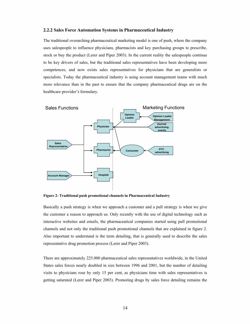
2.2.2 Sales Force Automation Systems in Pharmaceutical Industry
The traditional overarching pharmaceutical marketing model is one of push, where the company
uses salespeople to influence physicians, pharmacists and key purchasing groups to prescribe,
stock or buy the product (Lerer and Piper 2003). In the current reality the salespeople continue
to be key drivers of sales, but the traditional sales representatives have been developing more
competences, and now exists sales representatives for physicians that are generalists or
specialists. Today the pharmaceutical industry is using account management teams with much
more relevance than in the past to ensure that the company pharmaceutical drugs are on the
healthcare provider’s formulary.
Opinion LeaderManagement
Sales Representative
Account Manager
Physician
Pharmacist
Hospital
OpinionLeader
Journaladvertising.
events
Consumer DTC advertising
Sales Representative
Account Manager
Physician
Pharmacist
Hospital
OpinionLeader
Journaladvertising.
events
Consumer DTC advertising
Sales Functions Marketing Functions
Figure 2- Traditional push promotional channels in Pharmaceutical Industry
Basically a push strategy is when we approach a customer and a pull strategy is when we give
the customer a reason to approach us. Only recently with the use of digital technology such as
interactive websites and emails, the pharmaceutical companies started using pull promotional
channels and not only the traditional push promotional channels that are explained in figure 2.
Also important to understand is the term detailing, that is generally used to describe the sales
representative drug promotion process (Lerer and Piper 2003).
There are approximately 225.000 pharmaceutical sales representatives worldwide, in the United
States sales forces nearly doubled in size between 1996 and 2001, but the number of detailing
visits to physicians rose by only 15 per cent, as physicians time with sales representatives is
getting saturated (Lerer and Piper 2003). Promoting drugs by sales force detailing remains the

15
dominant approach, consuming 70 per cent of marketing budgets, which costs about 150 € per
sales representative visit (Lerer and Piper 2003).
Pharmaceutical companies aim to build sustainable partnership with target physicians, but this
must be achieved at the lowest possible cost, as margin pressure increases, companies are faced
with difficult resources allocation choices such as between putting more resources into gaining
market share in the highly competitive segment of high-prescribing physicians or developing
new market opportunities. The SFA systems are seen by the pharmaceutical companies as a
mean to improve the sales force effectiveness by helping the companies to determine the right
size for their sales force, targeting the key customers and get information from the field, all of
these at the lowest possible cost (Carpenter 2006; Lerer and Piper 2003). Looking to the high
costs of the sales forces in the pharmaceutical companies is easy to understand why in the late
1990s most of the original CRM systems in the pharmaceutical were focused in SFA tools.
The first SFA systems focused in the traditional push promotional systems exclusively in the
interaction of the sales functions with there clients (hospitals, pharmacists, physicians). The
initial SFA systems didn’t have any connection with the activities of the marketing functions
and there was no possibility of interaction and share of information between the push
promotional channels related to the sales functions and marketing functions (Carpenter 2006;
Lerer and Piper 2003).
The SFA are seen by the Pharmaceutical companies as the right mean to direct the sales forces
to the key customers and check the sales force performance. Pharmaceutical companies segment
their customers specially the physicians by their prescribing potential, these information can be
supplied at physician level in the United States by external vendors, but in Europe because of
legal restrictions the information is provided at territory level. In Europe because of the
restrictions the pharmaceutical companies rely on the sales representatives and their sales
managers to identify the physician’s high prescribers in their territories, and update the
information in the physician’s database in the SFA systems (Lerer and Piper 2003).
Another important use for the SFA systems is helping determine the size of the sales forces in
terms of sales representatives. Pharmaceutical companies usually buy an external database from
an external vendor with all the physician audience, if it is in the United States they might get
information about the number of prescriptions per physician but in Europe they will have to rely
in their internal available information about the physicians or if it is a completely new audience
they usually hire first the sales managers and a small number of reps to identify the high
16
prescribers and then hire the rest of the team according to the company needs (CGEY 2002;
Lerer and Piper 2003).
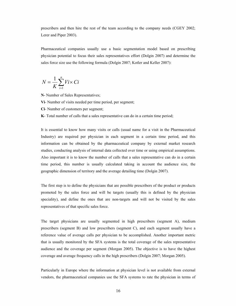
Pharmaceutical companies usually use a basic segmentation model based on prescribing
physician potential to focus their sales representatives effort (Dolgin 2007) and determine the
sales force size use the following formula (Dolgin 2007; Kotler and Keller 2007):
∑=
×=n
i
CiViK
N1
1
N- Number of Sales Representatives;
Vi- Number of visits needed per time period, per segment;
Ci- Number of customers per segment;
K- Total number of calls that a sales representative can do in a certain time period;
It is essential to know how many visits or calls (usual name for a visit in the Pharmaceutical
Industry) are required per physician in each segment in a certain time period, and this
information can be obtained by the pharmaceutical company by external market research
studies, conducting analysis of internal data collected over time or using empirical assumptions.
Also important it is to know the number of calls that a sales representative can do in a certain
time period, this number is usually calculated taking in account the audience size, the
geographic dimension of territory and the average detailing time (Dolgin 2007).
The first step is to define the physicians that are possible prescribers of the product or products
promoted by the sales force and will be targets (usually this is defined by the physician
speciality), and define the ones that are non-targets and will not be visited by the sales
representatives of that specific sales force.
The target physicians are usually segmented in high prescribers (segment A), medium
prescribers (segment B) and low prescribers (segment C), and each segment usually have a
reference value of average calls per physician to be accomplished. Another important metric
that is usually monitored by the SFA systems is the total coverage of the sales representative
audience and the coverage per segment (Morgan 2005). The objective is to have the highest
coverage and average frequency calls in the high prescribers (Dolgin 2007; Morgan 2005).
Particularly in Europe where the information at physician level is not available from external
vendors, the pharmaceutical companies use the SFA systems to rate the physician in terms of

17
prescribing potential, giving guidance to the sales representatives about how the range of
estimated prescriptions per month a sales representative should consider in order to classify a
physician in segment A, B or C in the company SFA system (Morgan 2005). The information is
usually updated periodically in the system, together with the targets for the number of calls and
coverage for the physicians in each segment (Dolgin 2007). This very simplistic segmentation
approach is the most commonly used by the pharmaceutical companies in their SFA systems
(CGEY 2002; Lerer and Piper 2003; Morgan 2005).
Generic pharmaceutical companies are also actively targeting pharmacists because in some
European countries they have the power to substitute brand drugs by generics when the generic
is available and because of this fact they have their SFA systems adapted also to target
pharmacists. Not only generic companies, but also pharmaceutical companies with OTC drugs
consider the pharmacist a key element, in this case because this type of pharmaceutical drugs
don’t require a medical prescription and the patient very often asks for advice to the pharmacist
(CGEY and INSEAD 2002).
The initial SFA systems were regarded by the salespeople as a mean more for management
information, entering data, command and control, than to aid the sales people in the field (Lerer
and Piper 2003).
More recent SFA systems are focusing in getting not only information in what the physicians
prescribe, but why they prescribe. Again the sales force is regarded as a very important source
of customer behavioural data in order to produce needs based segmentation models. The first
problem is that some sales representatives are not willing to share their customers in depth
knowledge built up over the years because they are afraid of losing power inside of the
organization (Lerer and Piper 2003). Another frequent problem is that the pharmaceutical
companies ask the sales representatives to enter data in the SFA systems about values,
behaviours and attitudes of physicians but at a certain point they struggle with large amounts of
data that is collected without clear rationale or strategy that produce a final output that is often
opaque and tenuous (CGEY and INSEAD 2002; Lerer and Piper 2003).
A basic classification of the data collected and incorporated in the CRM SFA systems and other
CRM components in today pharmaceutical environments is commonly accepted as (CGEY and
INSEAD 2002; Lerer and Piper 2003):
• Descriptive data: databases of customers including demographics, prescription behavior
(what they prescribe), professional status, etc..

18
• Activity data: sales calls, samples and promotional items, meetings and corporate events
invitations, requests for information and so on. This can be divided into activities of
various parties such as the sales representatives, physician and even the consumer.
• Sales data: this can be divided into company-generated (direct sales) or secondary
(external vendor like IMS) data.
• Profiling data: data specifically collected and used for segmentation purposes, it can be
for example, needs based data or behavior data collected directly from the SFA systems,
or through new channels like interactive web sites.
Even if the more recent CRM SFA systems generally have not been able to produce meaningful
physician’s needs-based segmentation models, they are incorporating more user-friendly
interfaces, and are linking the SFA systems to receive data from other functions such as
customer service or marketing, making the relationship between the sales representative and the
SFA system more interactive and productive (Carpenter 2006; Lerer and Piper 2003).
Many of the current CRM SFA systems are using new technologies to improve the effectiveness
of the sales rep work. The initial CRM systems required that every day the sales representative
had to update and connect through their computer at home all the information related to the
customer interaction during the day. Many of the current SFA systems offer the pharmaceutical
companies PDAs and Wireless PDAs with specific SFA software that can be used by the sales
representatives in the field to update directly the last call information in the PDA, for example
when they are waiting to be received by another physician (Carpenter 2006; Lerer and Piper
2003). Because only a small amount of sales representatives work time is spent in front of
customers, the rest is spent preparing, travelling, sitting in waiting rooms and doing
administrative time, the SFA mobile solutions are very well received by the sales
representatives as way to manage more effectively their time (Lerer and Piper 2003).
Another component that some SFA systems incorporate is an account management tool to be
used by the account managers particularly in the Hospital market (Dolgin 2007). More than the
frequency of calls made, this specific component focus in storing vital information collected by
the account managers about the account, objectives and activities developed by the account
managers in the accounts and behaviour information related to the different health professionals
that work in that account, and can influence the purchasing decisions in that specific health
institution.

19
2.2.3 CRM Programs focusing in online strategies and communication technologies
Online activities increasingly represent a diverse range of resources and applications including
websites, email, webcasts and others that are accessible 24 hours a day, seven days a week. The
pharmaceutical industry is using the online channel to develop specific CRM programs that
target health professionals or patients. Internet is a relatively inexpensive channel to develop
CRM programs compared to the traditional detailing done by the sales forces, what motivated
pharmaceutical companies to develop web based strategies to communicate with their costumers
(Bard 2007). In the United States where DTC advertising is allowed is frequent to see TV and
newspaper ads promoting a certain pharmaceutical drug and directing the consumer to a specific
product or pharmaceutical company website where the consumer can get more information
(Lerer and Piper 2003). This a good example of traditional channels working together with
online channels, that could be very useful to develop a more close relationship between the
consumer or patient and the pharmaceutical company (Lerer and Piper 2003).
The internet permits consumers in countries that ban DTC advertising to prescription
pharmaceutical drugs, like in Europe, to visit product websites in the United States and, despite
warnings found on pharmaceutical sites (saying that the information is exclusively for United
States citizens), there is little to prevent the free global transfer of consumer oriented
information on prescription drugs, giving to the European consumers the possibility to access
the same type of information about prescription drugs that the United States consumers receive
(Lerer and Piper 2003).
Some clinical trials require tens of thousands of participants and relying on investigators and
other physicians to identify and refer trial subjects is not a highly efficient approach. E-Clinical
trials it is a new process where a company uses Internet to recruit patients and uses web based
technology to establish effective communication between patients, investigators and the
pharmaceutical companies that sponsor the trial. This is a highly regulated area in terms of data
privacy, pharmaceutical companies are investing in E-Clinical Trials but their integration in a
company global CRM program is a topic that is not yet fully understood (Lerer and Piper 2003).
Pharmaceutical companies are using digital technologies to target health professionals and
patients. In the United States the pharmaceutical industry spent in 2005 an estimate of five
thousand million dollars in DTC, mainly in TV ads, but the lasts surveys done shown that the

20
public in the United Sates believes that too much money is spent in DTC, and part of this money
could be spent in making pharmaceutical drugs more affordable (Datamonitor 2006).
The pharmaceutical companies are investing both in Europe and United States in internet sites
targeting the patients, in the case of United States this approach is now regarded as being
considerable more affordable than investing in TV advertising, because more than 35% of all
internet users, survey the web to search for health information (Lerer and Piper 2003).
The local European web sites of pharmaceutical companies, avoid doing DTC advertising of
prescription drugs, but in some conditions the pharmaceutical companies can provide non-
promotional information about drugs for chronic diseases and they are allowed to answer to
specific questions posted in a web site or by email to a patient that is taking a pharmaceutical
drug supplied by the company if the answer is provided by a health professional working for the
pharmaceutical company (Lerer and Piper 2003).
Currently almost all pharmaceutical companies have product-focused or disease specific
websites aiming the consumer or patient. In Europe because of the ban on DTC the local
European websites focus in disease awareness campaigns using unbranded health information,
nevertheless many use creative procedures to overcome the regulation limitation (Lerer and
Piper 2003). A good example is the pharmaceutical company Organon that avoids mentioning
in their European websites the brand names of their pharmaceutical drugs, but when they are
talking about hormonal contraceptive vaginal ring, they are obviously talking about Nuvaring®
their own product because this is the only contraceptive of it’s kind in Europe without
mentioning the contraceptive brand name, they are promoting a contraceptive option that they
are the sole providers.
In the case of OTC in Europe it is possible to have product specific websites, and they have
already been implemented by several pharmaceutical companies to promote directly their
brands to the public. In the United States the internet is a channel used to DTC, so it is frequent
to have website that promote a pharmaceutical drug and disease awareness and the same time.
In the United states it’s possible to have a pharmaceutical company corporate website that have
all this features or in other cases the pharmaceutical companies have separate product websites
(Lerer and Piper 2003).
The internet allowed a very important channel for the pharmaceutical companies to interact with
the patients and develop patient relationship management (PRM) programs. PRM can be
regarded as consumer or patient focused CRM. Current PRM solutions in pharmaceutical

21
industry are designed to either support lifestyle programmes, such as smoking cessation and
weight reduction or for chronic diseases (Lerer and Piper 2003). In the next sections specific
European and American examples of PRM are described.
The American Medical Association released findings that showed that many of the United
States physicians in 2001, about 80%, were using internet (Lerer and Piper 2003) for medical
research and other professional activities, being a very common tool today for the vast majority
of the them, in Europe the initially acceptance as not so big like the United States, but now is
also a very important tool for the European physicians, with high acceptance (Bard 2007). In a
recent survey in Europe even if generally the physicians still consider the sales representative as
a very important source of information, yet 50 per cent of all survey responders admit that they
prefer to receive information electronically; via email, webcasts, product sites or corporate sites
provided directly by pharmaceutical companies.
E-detailing is one of the activities that the pharmaceutical companies are incorporating in their
websites, or even in PDA or laptop to help the sales representative in their detailing process. E-
detailing is the digital enablement of information delivery to health professionals, creating new
digital channels for interaction between the pharmaceutical company and the physicians (Lerer
and Piper 2003). A recent survey shown that e-detailing is already reaching regularly more than
50 per cent of the American physicians, where in Europe the market is still relatively young in
terms of development and uptake, with less than 40 per cent of European physicians saying that
they have participated in an e-detailing programme in the past 12 months (Bard 2007).
Physicians portals are typical implementations of eCRM programs that can be incorporated in
the company corporate website or be a stand alone website. These websites are only accessible
to physicians or in some cases also other health professionals and require a previous registration
and only after a check-up process to confirm if it is really a certified health professional the user
will receive a password to access the areas in the website that are reserved to health
professionals.
A recent survey indicates that 38 per cent of physicians who regularly go on-line say they
frequently change their prescribing behaviour as a result of information they have accessed
electronically (Bard 2007).
Some companies are also adopting Customer Service Center (CSC) multi-channel strategies as
part of an improved CRM package, using Internet, automated response, web tools, as compared
to previously CSC being almost exclusively telephone-based (Lerer and Piper 2003).

22
Others industries, like for example consumer goods used e-tools, to collect information about
the consumers and get a deeper understanding about their needs. In the area of analytics and
customer understanding using e-tools in the pharmaceutical industry one report mentioned that
only two or three companies are getting positive results without mentioning their name, but
saying that they are the exceptions (Lerer 2002). Again without using the correct analytics the
pharmaceutical industry can’t maximize the return of their CRM investments.
2.2.4 CRM focusing in Supply Chain and Demand Management Integration
In some specific pharmaceutical companies after the implementation of ERP systems, they took
the opportunity to make the integration of supply chain and demand chain elements (Oracle and
Peppers&Rogers Group 2007).
Pharmaceutical companies that deal with products of low differentiation, such as generic
products, medical devices and some types of hospital products see an effective integration of
supply chain and demand a very effective way of saving money by optimizing their supply
chain and at the same time deliver high quality services that increase their sales revenue (Oracle
and Peppers&Rogers Group 2007).
A good example is Baxter Medication Delivery a division of Baxter, a global provider of
medical products and services. Baxter Medication delivery packages up and ships a host of
products such as Intravenous (IV) solutions and frozen drugs to hospitals and physician offices
and it also negotiates with Group Purchasing Organizations on behalf of clients (Oracle and
Peppers&Rogers Group 2007).
Baxter Medication Delivery Operation Manager and CRM lead stated that the product line and
competitive pricing are always going to be important, but what really sets the brand are the
service and support that come with those products (Oracle and Peppers&Rogers Group 2007).
Baxter products are the type of products of low differentiation that require a very effective
supply chain management, we are talking about IV solutions and frozen drugs, that require very
effective supply because any failure in the supply chain can damage the products irreversibly.
Baxter CRM solutions used a SFA system that enables the sales representative to have access to
the company product stocks and orders per customer, information about contract compliance, to
know if the customer is buying what was agreed, and also to feedback customer requests to the

23
customer service. The implementation of the system also enabled the company to better forecast
their future sales and to better plan the manufacturing of products (Oracle and Peppers&Rogers
Group 2007).
2.2.5 Differences between the current CRM programs in Europe and United States
The possibility to make direct-to-consumer advertising in the United States enabled the
pharmaceutical industry to develop more sophisticated CRM programs than in Europe. A good
example it’s a loyalty program implemented by Novartis in United States. The program is
known as BP Success Zone and started in 2004 and promotes directly to the patients, the need
for them to take medication for controlling their Blood pressure. For enrolling in the program
they also need to be prescribed with a Novartis blood pressure medication by their physician.
Then the patient can request the physician a BP Success Zone Kit in order for him to receive the
program benefits. But first the patient needs to activate their Kit, and for that he needs to fill a
formulary in the internet or do the registration via a call center. The Kit consists of a free sample
for one month of medication, a Membership Card for Program discounts and benefits that
includes a 10 dollar discount per pack in any pharmacy and a free Omron® monitor for blood
pressure measurement, ongoing support materials and website access with specific tools for the
program, finally also includes a money back guarantee where patients can receive from
Novartis, reimbursement for up to 4 months of out-of-pocket drug costs if, after taking the
maximum dose of Novartis medication for at least 30 days their blood pressure is not controlled
to the goal determined by their healthcare professional they can use a Guarantee Affirmation
Form to get the money back, signed by their healthcare professional, stating that the patient was
not able to reach the blood pressure goal set by him (Novartis 2007).
This is a typical implementation of a loyalty program for a chronic disease with a concept
similar with other examples seen for example in the consumer industry. This example basically
demonstrates the biggest difference between the CRM programs in Europe and United States,
the fact that the focus in the patient in the United States is bigger and deeper than in Europe in
terms of CRM programs. In the last European Sales Force Effectiveness Summit for
Pharmaceutical industry held in 2006 (Eyeforfarma 2006), CRM was the main topic, but almost
all the European CRM approaches presented where focused in the physician and in improving
CRM SFA tools. The analytics presented to support the European CRM system were extremely
poor, segmentation methodologies were very rudimentary, for example physician segmentation
presented was based on empirical rules without any statistical validation. We can resume that
CRM programs in Europe were developed around physicians as the main target, with some

24
examples of internet use to target patients in contrast with more sophisticated CRM programs in
United States targeting the patients, and CRM programs targeting the physicians and other
health care professionals. The literature review indicates that the CRM programs in the
pharmaceutical industry focus separately health professionals and patients specially in Europe
that fact seems to be evident, in the United States the last examples like the one above
described, gives an indication that some linking could be already happening but without
consistent evidence to support it.

25
3. METHODOLOGY ______________________________________________________________________
3.1 BUSINESS PURPOSE OF APPLIYING MULTIVARIATE TECHNIQUES IN PHARMACEUTICAL CRM.
______________________________________________________________________
The so-far-described CRM approach does not yet seem completely adapted to the complexity of
the health care industry as many players are involved in the health care process, not just the
physician and the patient, and each are having an increasingly defined role. Nevertheless the
United States seems to be more advanced than Europe, probably because the legislation in the
United States it’s more liberal, allowing DTC advertising and the possibility to get prescribing
information per physician. Also in the pharmaceutical marketing the product focus approach it
is still dominant versus the customer centric approach, what is a clear obstacle to the success of
a CRM program.
Another important issue in pharmaceutical industry is the poor analytics applied to the current
CRM programs, probably because CRM is not regarded as a market research tool and the non-
involvement of market research departments in the project leads to a loss of analytical potential
for the CRM programs. Basically the poor use of analytics in CRM in the pharmaceutical
industry is one of the big obstacles to the success of CRM programs in this business area.
By identifying the issues it’s possible to take several approaches in order to improve the
pharmaceutical industry CRM programs, but this thesis will focus in one specific, but very
important topic, in demonstrating the overall usefulness of using exploratory multivariate
statistical techniques, and their exemplified use in a dataset from a Pharmaceutical CRM system
belonging to a company that operates in the Portuguese hospital pharmaceutical market,
focusing by this way in the European perspective of CRM in the pharmaceutical industry. By
using multivariate techniques we will demonstrate their usefulness in pharmaceutical CRM and
support the idea that the pharmaceutical companies should focus in implementing them in their
current CRM programs in order to increase sales and marketing effectiveness according to the
objectives defined in this thesis.
Considering the importance of analysing the current complexity of the pharmaceutical market,
and so, the importance of studying the relationships among sets of interrelated variables, and the

26
identification of factors that explain the correlations among them, makes factor analysis a very
suitable and appropriate technique to be used in a analysis that can explain the business
dynamics in the pharmaceutical market. It can also be useful to produce a new, smaller set of
uncorrelated variables to replace an original set of correlate variables in subsequent multivariate
analysis, such as cluster analysis.
Another important technique to be used in this thesis is cluster analysis, considering the poor
segmentation techniques currently employed in most of the CRM programs in the
pharmaceutical industry, particularly at European level, cluster analysis can improve the quality
of the segmentations. The primary objective of cluster analysis is to classify objects into
relatively homogeneous groups based on a set of variables. In this thesis, cluster analysis will be
used to segment the Hospitals in the CRM file used. Hierarchical techniques and Self-
Organizing Maps (SOMs) will be used. SOMs are known by their ability to deal well with large
amounts of data and it’s robustness to outliers. The use of both types of techniques will be
commented.
No multivariate techniques were ever applied to the dataset used in this thesis and also because
of the relative small size in terms of variables and observations of the dataset, make possible
and useful the use of exploratory multivariate techniques like hierarchical clustering or factor
analysis which are traditional market research techniques together with a data mining technique
like SOMs.
3.2 DESCRIPTION OF THE CRM DATA FILE USED. ______________________________________________________________________
A CRM file with 73 observations and 10 variables was provided to be used in this thesis by
Tactimed a consultancy company for the pharmaceutical industry. The observations correspond
to 73 Hospitals that are clients of a pharmaceutical industry in Portugal that operates in the
Oncology Hospital Market. One variable is a nominal variable and classifies the Hospitals by
regions (North, Center and South) the other nine variables used in the analysis are all
quantitative variables (ratio scale data) and are related to the sales representatives activities
(number of visits made to the health professionals in each hospitals), total number of
chemotherapy patients treated in each hospital, and total packs of each oncology company
product sold per hospital. The time period in analysis is the year 2004. For confidentiality
reasons the name of the pharmaceutical company will not be revealed or the products names,

27
but a brief description of each product will be provided. In Portugal IMS does not provide any
market share data per hospital, and for that reason no information about competitors is provided
in the file. In this file it is possible to have patient data (chemotherapy patients), sales
representative activity data, and product sales data, and by studying the relationships between
these different variables that together are critical for the success of a pharmaceutical company, it
will be possible to provide valuable business insights. A summary description of the
quantitative variables present in the data is provided:
Variable name Description
Total Calls Number of visits made by the company sales representatives to
the health care professionals in each Hospital.
Total Guideline Number of defined target visits per Hospital to be achieved by
the sales representatives.
Patients Number of chemotherapy patients treated in each Hospital
Product A It is a standard Oncology therapy. The variable is measured in
packs (units).
Product B It is an innovative oncology product. The variable is measured in
packs (units).
Product C It is a standard support therapy. The variable is measured in
packs (units).
Product D It is an innovative hemato-oncology product. The variable is
measured in packs (units).
Product E It is an innovative and recent hemato- oncology therapy with the
same therapeutic indication than Product D, but with a more
convenient administration schedule and slightly more expensive.
The variable is measured in packs (units).
Product F It is an innovative Hemato- Oncology therapy that by its
specificity can only be used in specific hospitals with the right
storing conditions. The variable is measured in packs (units)
Table 2- CRM dataset variables measured in 2004.
The innovative products have a cost per unit that is more expensive than the other products.
To conduct the analysis Microsoft Excel and the statistic software’s SPSS 11, and MatLab 7.0
with SOM_TOOLBOX were used in this thesis. EndNote was used to create bibliographic
references.

28
3.3 FACTOR ANALYSIS ______________________________________________________________________
Factor analysis was originally developed to explain student performance in various courses and
to understand the link between grades and intelligence. Spearman in 1904 hypothesized that
students' performances in various courses are intercorrelated and their intercorrelations could be
explained by students' general intelligence levels. The main objective of factor analysis is to
search or identify the underlying factor(s) or latent constructs that can explain the
intercorrelation among the variables (Sharma 1996). But factor analysis can also be used to
(Vilares and Coelho 2005):
- Identify a new set of variables, smaller in number, non-correlated that substitute the
original correlated variables in subsequent multivariate analysis (ex: regression analysis,
cluster analysis).
- Select a small set of salient variables from a larger set to be used in subsequent
multivariate analysis.
3.3.1 Factor Model
Consider a p-indicator m-factor model given by the following equations (Sharma 1996):
xι = λ11ξ1 + λ 12ξ2 +….+ λ1mξm + εl x2 = λ21ξ1+ λ 22ξ2 +….+ λ2mξm + ε2 . . xρ = λρ1ξ1 + λρ2ξ2 +….+ λpmξm + εp , (3.3.1)
where xι, x2,……, xρ are indicators of the m factors, λpm is the pattern loading of the pth variable on
the m factor, and εp is the unique factor for pth variable. The indicators and the common factor
are standardized. In these equations the intercorrelation among the p indicators is being
explained by the m common factors. It is usually assumed that the number of common factors,
m, is much less than the number of indicators, p. In other words, the intercorrelation among the
p indicators is due to a small (m < p) number of common factors. The number of unique factors
is equal to the number of indicators. In this model the unique factors (εp) are independent and
identically distributed with zero mean and variance Ψi and the common factors (ξm) and the
unique factors (εp) are independent. If the common factors are not correlated the factor model is

29
referred to as an orthogonal model, and if they are correlated it is referred to as an oblique
model (Vilares and Coelho 2005). In this thesis only orthogonal models will be used.
The variance of any variable x is given by (Sharma 1996): Var(x) = λi1
2 + λi22 + ……+ λim
2 + Ψi (3.3.2)
The variance of any given variable x can be divided in two components; where hi2= λi1
2 + λi22 +
……+ λim2, is the communality of x, an estimation of the variance of x explained by the
common factors and Ψi is the variance portion that is unique belonging to variable x.
Eq. (3.3.1) can be represented in matrix form as:
x = Λξ + ε, (3.3.3)
where x is a p × 1 of variables, Λ is a p × m matrix of factor pattern loadings, ξ is a m × 1 vector
of unobservable factors, and ε is p × 1 vector of unique factors. Eq. (3.3.3) is the basic factor
analysis equation. It will be assumed that the factors are not correlated with the error
components, and without loss of generality it will be assumed that the means and variances of
variables and factors are zero and one, respectively. The correlation matrix, R, of the indicators,
since the data are standardized, the correlation matrix is the same as the covariance matrix, is
given by:
Ε(xx’) = E [(Λξ + ε) (Λξ + ε)’]
= E [(Λξ + ε) (Λ’ξ’ + ε’)]
= E (Λξξ’Λ’ ) + E (ε ε’)
R = ΛΦΛ' +Ψ, (3.3.4)
where R is the correlation matrix of the observables, Λ is the pattern loading matrix., Φ is the
correlation matrix of the factors, and Ψ a diagonal matrix containing the unique variances. The
communalities are given by the diagonal of R-Ψ matrix. The off-diagonals of the matrix R give
the correlation among the indicators. Λ,Φ, and Ψ matrices are referred to as parameter matrices
of the factor analytic model, and it is clear that the correlation matrix of the observables is a
function of the parameters. The objective of factor analysis is to estimate the parameter matrices
given the correlation matrix.
For an orthogonal factor model, Eq. (3.3.4) can be rewritten as
R = ΛΛ' +Ψ, (3.3.5)

30
If no a priori constraints are imposed on the parameter matrices then we have exploratory factor
analysis; a priori constraints imposed on the parameter matrices result in a confirmatory factor
analysis.
The correlation between the indicators and the factors is given by:
Ε(xξ’) = E [(Λξ + ε) ξ’]
= Λ E(ξ ξ’) + E(ε ξ’)
A = Λ Φ, (3.3.6)
where A gives the correlation between indicators and factors. For an orthogonal model,
A = Λ (3.3.7)
Again, it can be clearly seen that for an orthogonal factor model the pattern loadings are equal
structure loadings and are commonly referred to as the loadings of the variables.
3.3.2 Factor Indeterminacy
In exploratory factor analysis the factor solution is not unique. A number of different factor pat-
tern loadings and factor correlations will produce the same correlation matrix for the indicators.
Mathematically it is not possible to differentiate between the alterative factor solutions, and this
is referred to as the factor indeterminacy problem. Factor indeterminacy results from two
sources: the first pertains to the estimation of the communalities and the second is the problem
of factor rotation. Each is described below (Sharma 1996).
Communality Estimation Problem
Eq. (3.3.5) can be rewritten as
ΛΛ’ = R -Ψ. (3.3.8)
This is known as the fundamental factor analysis equation. Note that the right-hand side of the
equation gives the correlation matrix with the communalities in the diagonal. Estimates of the or

31
loadings (i.e Λ ) are obtained by computing the eigenstructure of the R – Ψ matrix. However the
estimate of Ψ is obtained by solving the following equation:
Ψ = R - ΛΛ’ (3.3.9)
That is, the solution of Eq. (3.3.8) requires the solution of Eq. (3.3.9), but the solution of Eq.
(3.3.9) requires the solution of Eq.(3.3.8). It is this circularity that leads to the estimation of
communalities problem.
Factor Rotation Problem Once the communalities are known or have been estimated, the parameter matrices of the factor
model can be estimated. However, one can obtain a number of different estimates for Λ and Φ
matrices. Geometrically, this is equivalent to rotating the factor axes in the factor space without
changing the orientation of the vectors representing the variables. For example, suppose we
have any orthogonal matrix C such that C'C = CC' = I. Rewrite Eq. (3.3.4) as
R = ΛCC’Φ CC'Λ' + Ψ
= Λ* Φ* Λ*’ + Ψ, (3.3.10)
where Λ* = ΛC and Φ* = C’ΦC. As can be seen, the factor pattern matrix and the correlation
matrix of factors can be changed by the transformation matrix, C, without affecting the
correlation matrix of the observables. And, an infinite number of transformation matrices can be
obtained, each resulting in a different factor analytic model. Geometrically, the effect of
multiplying the Λ matrix by the transformation, C, is to rotate the factor axes without changing
the orientation of the indicator vectors. This source of factor indeterminacy is referred to as the
factor rotation problem. One has to specify certain constraints in order to obtain a unique esti-
mate of the transformation matrix, C. Some of the constraints common1y used are discussed in
the following section.
3.3.3 Factor Rotations
Rotations of the factor solution are the common type of constraints placed on the factor model
for obtaining a unique solution. There are two types of factor rotation techniques: orthogonal
and oblique. Orthogonal rotations result in orthogonal factor models, whereas oblique rotations
result in oblique factor models. Both types of rotation techniques are discussed below (Sharma
1996).

32
Orthogonal Rotation ln an orthogonal factor model it is assumed that Φ = I. Orthogonal rotation technique involves
the identification of a transformation matrix C such that the new loading matrix is given by Λ*
= ΛC and
R = Λ* Λ*’.
The transformation matrix is estimated such that the new loadings result in an interpretable
factor structure. Quartimax and varimax are the most commonly used orthogonal rotation
techniques for obtaining the transformation matrix.
Figure 3- Projection of vectors onto a two-dimentional space in a orthogonal factor model
The projection of a vector onto an axis gives the component of the point representing the vector
with the respect to that axis. These components (i.e., projections of the projection vectors) are
the structure loadings and also the pattern loadings for orthogonal factor models.
Quartimax Rotation The objective of quartimax rotation is to identify a factor structure such that all the indicators
have a fairly high loading on the same factor; in addition, each indicator should load on one
other factor and have near zero loadings on the remaining factors. This objective is achieved by
maximizing the variance of the loadings across factors, subject to the constraint that the
communality of each variable is unchanged. Thus, suppose for any given variable i, we define
( )m
Qiiij
m
j
22.
21
λλ −=
∑ = , (3.3.11)

33
where Qi; is the variance of the communalities (i.e., square of the loadings) of variable i, λij2 is
the squared loading of the ith variable on the jth factor, λi2. is the average squared loading of the
ith variable, and m is the number of factors. The preceding equation can be rewritten as
2
1
2
1
24
m
mQi
m
j
m
jijij∑ ∑=
=⎟⎟⎠
⎞⎜⎜⎝
⎛−
=
λλ (3.3.12)
The total variance of the variables is given by:
( )
∑∑ ∑
∑=
= =
= ⎥⎥⎥
⎦
⎤
⎢⎢⎢
⎣
⎡ −==
p
i
m
j
m
j ijijp
i m
mQiQ
12
1
2
124
1.
λλ (3.3.13)
For quartimax rotation the transformation matrix, C, is found such that Eq. (3.3.11) is
maximized subject to the condition that the communality of each variable remains the same.
Note that once the initial factor solution has been obtained, the number of factors, m, remains
constant. Furthermore, the second term in the equation, ( )∑ =
m
j ij12λ , is the communality of the
variable and, it will also be a constant. Therefore maximization of Eq. (3.3.11) reduces to
maximizing the following equation:
∑∑==
=m
jij
p
iQ
1
4
1λ (3.3.14)
In most cases, prior to performing rotation the loadings of each variable are norma1ized by di-
viding the loading of each variable by the total communality of the respective variable.
Varimax Rotation
The objective of varimax rotation is to determine the transformation matrix, C, such that any
given factor will have some variables that will load very high on it and some that will load very
low on it. This is achieved by maximizing the variance of the squared loading across variables,
subject to the constraint that the communality of each variable is unchanged. That is, for any
given factor:

34
( )
pV
p
i jijj
∑ =−
= 1
22.
2 λλ
=( )
21
2
124
pp p
i
p
i ijij∑ ∑= =− λλ
(3.3.15)
Where Vj is the variance of the communalities of the variables within factor j and 2. jλ is the
average squared loading for factor j. The total variance for all the factors is then given by:
∑=
=m
jjVV
1
= ( )
∑ ∑ ∑=
= =
⎟⎟⎟
⎠
⎞
⎜⎜⎜
⎝
⎛ −m
j
p
i
p
i ijij
pp
12
1
2
124 λλ
= ( )
21
2
12
1 14
pp
m
j
p
i ijm
j
p
i ij ∑ ∑∑ ∑ = == = −λλ
(3.3.16)
Since the number of variables remains the same, maximizing the preceding equation is the same
as maximizing
( )
ppV
m
j
p
i ijm
j
p
iij
∑ ∑∑∑ = =
= =
−= 1
2
12
1 1
4λ
λ (3.3.17)
The orthogonal matrix, C, is obtained such that Eq. (3.3.17) is maximized, subject to the con-
straint that the communality of each variable remains the same. Equamax Rotation The Equamax approach, a commonly used method in marketing, is used as a compromise
between two frequently used methods, Quartimax and Varimax. In practice, the objective of all
methods of rotation is to simplify the rows and columns of the factor matrix to facilitate
interpretation. Rather than concentrating either on simplification of the rows or simplification of
the columns, the Equamax approach tries to accomplish some of each.

35
( )
pmpV
m
j
p
i ijm
j
p
iij
∑ ∑∑∑ = =
= =
−= 1
2
12
1 1
4
2
λλ (3.3.18)
Overall consideration about orthogonal rotations.
It is clear from the preceding discussion that quartimax rotation maximizes the total variance of
the loadings row-wise and varimax maximizes it column-wise. It is therefore possible to have a
rotation technique that maximizes the weighted sum of row-wise and column-wise variance.
That is, maximize
Z = αQ + βpV, (3.3.19)
Where Q is given by Eq. (3.3.14) and pV is given by Eq. (3.3.17). Considering the following
equation:
( )p
m
j
p
i ijm
j
p
iij
∑ ∑∑∑ = =
= =
− 1
2
12
1 1
4λ
γλ (3.3.20)
Where γ = β/(α + β).
Different values of γ results in different types of rotation. Specially, the above criterion reduces
to a quartimax rotation if γ = 0 (i.e., α = 1; β = 0), reduces to a varimax rotation if γ = 1 (i.e., α =
o; β = 1), reduces to an equimax rotation if γ = m/2, and reduces to a biquartimax if γ = 0.5
(i.e., α = 1; β = 1).
Oblique Rotation
In oblique rotation the axes are not constrained to be orthogonal to each other. In other words, it
is assumed that the factors are correlated (i.e., Φ ≠ I). The pattern loadings and structure
loadings will not be the same, resulting in two loading matrices that need to be interpreted. The
projection of vectors or points onto the axes, which will give the loadings, can be determined in

36
two different ways. In Figure 4 the projection is obtained by dropping lines parallel to the axes.
These projections give the pattern loadings (i.e. λ's ). The square of the pattern loading gives the
unique contribution that the factor makes to the variance of an indicator.
Figure 4- Oblique factor model-pattern loading
In Figure 5 projections are obtained by dropping lines perpendicular to the axes. These
projections give the structure loadings. As seen previously, structure loadings are the simple
correlations among the indicators and the factors. The square of the structure loading of a
variable for any given factor measures the variance accounted for in the variable jointly by the
respective factor and the interaction effects of the factor with other factors. Consequently,
structure loadings are not very useful for interpreting the factor structure. It has been recom-
mended that the pattern loadings should be used for interpreting the factors.
Figure 5- Oblique factor model- structure loading
The coordinates of the vectors or points can be given with respect to another set of axes,
obtained by drawing lines through the origin perpendicular to the oblique axes. In order to dif-
ferentiate the two sets of axes, the original set of oblique axes is called the primary axes and the
new set of oblique axes is called the reference axes. Figure 6 gives the two sets of axes. It can be
clearly seen from the figure that the pattern loadings of the primary axes are the same as the
structure loadings of the reference axes, and vice versa. Therefore, one can either interpret the
pattern loadings of the primary axes or the structure loadings of the reference axes.

37
Figure 6- Oblique factor model-pattern and structure loadings
Interpretation of an oblique factor model is not very clear, therefore oblique rotation techniques
are not very popular, and will not be subject to use in this thesis (Sharma 1996).
3.3.4 Data Matrix
The most common data matrix in factor analysis is the correlation matrix, that corresponds to an
analysis to the variables centered and reduced, that as be the one used in the discussion above.
This method is particularly important when we want to avoid those variables with a larger scale to
influence the structure of produced factors (Vilares and Coelho 2005).
If we don’t consider the standardization of the observed variables, Eq. (3.3.3), can be written as:
x = μ + Λξ + ε, (3.3.21)
Another option is to use the covariance matrix. In this option only the mean is removed to
produce this matrix, and this option is interesting when is possible to accept that the variables
have similar variances (or when we want explicitly to consider the variance differences in
producing the factors), but we want to remove the differences between the medium values of the
variables. A third alternative is to use a non mean corrected covariance matrix, and this can be a
good option if the scales are all in the same metric and have approximately the same medium
level or if we want to consider the variances and level differences in the original variables to
produce the factors. (Vilares and Coelho 2005).
3.3.5 Factor Extraction Methods
The two most popular exploratory factor analysis extraction methods are principal components

38
factoring (PCF) and principal axis factoring (PAF). In most cases, there is very little difference
between the results of PCF and PAF, therefore in most of the cases it really does not matter
which of two techniques is used (Sharma 1996). However, there are conceptual differences
between the two methods that will be explained further bellow.
Maximum likelihood estimation procedure is not commonly used in exploratory factor analysis
and the procedure assumes that the data comes from a multivariate normal distribution, and is
used in confirmatory factor analysis. Other techniques not used in this thesis like image
analysis, unweighted least-squares factoring, generalized least-squares factoring and alfa factor
analysis, will also be briefly mentioned (Sharma 1996).
Principal Components Factoring (PCF) PCF assumes that the prior estimates of communality are one. The correlation matrix is then
subjected to a principal components analysis. The principal components solution is given by:
ξ = Λx (3.3.22)
where ξ is a p × 1 vector of principal components, Λ is a p × p matrix of weights to form the
principal components, and x is p × 1 vector of p variables. The weight matrix, Λ, is an
orthonormal matrix. That is, Λ’Λ = ΛΛ’ = I. Premultiplying Eq. (3.3.22) results in
Λ’ξ = Λ’Λx, (3.3.23)
or
x = Λ’ ξ (3.3.24)
As can be seen above, variables can be written as functions of the principal components. PCF
assumes that the first m principal components of the ξ matrix represent the m common factors
and the remaining p - m principal components are used to determine the unique variance.
Principal Axis Factoring (PAF)
PAF essentially reduces to PCF with iterations. In the first iteration the communalities are
assumed to be one. The correlation matrix is subjected to a PCF and the communalities are
estimated. These communalities are substituted in the diagonal of the correlation matrix. The
modified correlation matrix is subjected to another PCF. The procedure is repeated until the
estimates of communality converge according to a predetermined convergence criterion. PAF

39
implicitly assumes that a variable is composed of a common part and a unique part, and the
common part is due to the presence of common factors. That is PAF technique assumes an
implicit underlying factor model.
The iteration process is described bellow (Sharma 1996):
Step 1: First it assumed that the prior estimates of the communalities are one. A PCF solution is
then obtained. Based on the number of components (factors) retained, estimates of structure or
pattern loadings are obtained which are then used to reestimate the communalities.
Step 2: The maximum change in estimated communalities is computed. It is defined as the
maximum difference between previous and revised estimates of the communality for each
variable. Note that it was assumed that the previous estimates of communalities are one.
Step 3: If the maximum change in the communality is greater than a predefined convergence
criterion, then the original correlation matrix is modified by replacing the diagonals with the
new estimated communalities. A new principal components analysis is done on the modified
correlation matrix and the procedure described in Step 2 is repeated. Steps 2 and 3 are repeated
until the change in the estimated communalities is less than the convergence criterion.
In SPSS PAF is not more than Principal-axis factoring with iterated communalities or Iterated
principal factor analysis and the PAF procedure used in this thesis is an iterated procedure,
because we used SPSS.
Image Analysis In image analysis, the communality of a variable is defined as the square of the multiple
correlation obtained by regressing the variable on the remaining variables. That is, there is no
indeterminacy due to the estimation of the communality problem. The squared multiple
correlations are inserted in the diagonal of the correlation matrix and the off-diagonal values of
the matrix are adjusted so that none of the eigenvalues are negative.
Alpha Factor Analysis
In alpha factor analysis it is assumed that the data are the population, and the variables are a
sample from a population of variables. The objective is to determine if inferences about the

40
factor solution using a sample of variables holds for the population of variables. That is, the
objective is not to make statistical inferences, but to generalize the results of the study to a
population of variables. This technique is rarely used (Sharma 1996),
Maximum likelihood
This procedure assumes that the data comes from a multivariate normal distribution. The
solutions of Λ and Ψ are obtained by the minimization of the function:
( )[ ] ( ) ptrF −+ΛΛ−+ΛΛ=−− R'log R' 1212 ψψ (3.3.25)
Where tr is the trace of the matrix (i.e., the sum of the diagonal elements) and | | the determinant
of the matrix (Johnson and Wichern 1998).
Unweighted least squares factoring
Unweighted least squares factoring is based on minimizing the sum of squared differences
between observed and estimated correlation matrices, not counting the diagonal.
Generalized least squares factoring
Generalized least squares factoring is based on adjusting unweighted least squares factoring by
weighting the correlations inversely according to their uniqueness (more unique variables are
weighted less).
3.3.6 Methods to evaluate if data is appropriate for factor analysis
As one of the aims of factor analysis is to find factors that make it possible to explain the
correlations among variables, these variables must correlate with each other for the model to be
appropriate. Bartlett’s sphericity test can be used to test the hypothesis that the correlation
matrix is an identity matrix, consisting of the χ2 test (chi-squared transformation) of the
determinant of the correlation matrix. Nevertheless Bartlett’s is sensitive to sample size
meaning that for large samples one is liable to conclude that the correlation matrix departs from
orthogonality even when the correlations between the variables are small (Vilares 2005 and
Coelho 2005).

41
Another better way to test the appropriateness of the factor analysis is by means of the Kaiser-
Meyer-Olkin measurement (KMO), which compares the values of the coefficients of correlation
observed with the values of the partial correlation coefficients, which is calculated as follows:
∑ ∑∑ ∑
∑ ∑−
= +=
−
= +=
−
= +=
+= 1
1 1
21
1 1
2
1
1 1
2
0|
p
i jixxx
p
i
p
ijxx
p
i
p
ijxx
jiji
ji
rr
rKMO (3.3.26)
where ji xxr is the coefficient of simple correlation among the variables xi and xj, and 0
|xxx jir
is
the coefficient of partial correlation among the variables xi e xj. A low KMO value indicates that
the correlations between the pairs of variables could not be explained by other variables and
consequently factor analysis should not be used. KMO can be calculated not only at global level
but also for each of the variables in the analysis. (Vilares and Coelho 2005).
Although there are no statistical tests for the KMO measure, the following guidelines are
suggested (Sharma 1996).
KMO Measure Recommendation
≥ 0,90 Marvelous
> 0,80 Meritorious
> 0,70 Middling
> 0,60 Mediocre
> 0,50 Miserable
≤ 0,50 Unacceptable
Table 3- KMO measure of appropriateness for factor analysis
We can also examine the partial correlations controlling for other variables. These correlations,
also referred as negative anti-image correlations, should be small for the correlation matrix to be
appropriate for factoring. However, how small, is small is essentially a judgmental question
(Sharma 1996).
3.3.7 Determining the number of factors

42
The most popular heuristics are eigenvalue greater than one rule, total variance explained and
the scree plot. Several methods are described below to determine the number of factors but
interpretability should be one of the most important criteria in determining the number of
factors together with the other methods (Sharma 1996; Vilares and Coelho 2005).
Scree test
The scree test is a graphical technique attributed to Cattell who described it in term of retaining
the correct number of factors in a factor analysis. While a scree graph is simple to construct, its
interpretation may be highly subjective. Let λk represent the k-th eigenvalue obtained from a
covariance or correlation matrix. A graph of λk against k is known as a scree graph. The location
on the graph where a sharp change in slope occurs in the line segments joining the points is
referred to as an elbow. The value of k at which this occurs represents the number of
components that should be retained. Nevertheless interpretation might be confounded in cases
where the scree graph either does not have a clearly defined break or has more than one break.
Also, if the first few roots are widely separated, it may be difficult to interpret where the elbow
occurred due to a loss in detail caused by scaling (Sharma 1996).
Figure 7- Cattell's scree test example
In the example above since the first inflection point occurs between the fourth and fifth
eigenvalues, the implied dimension is five.
Average eigenvalue (Guttman-Kaiser rule and Jolliffe's Rule)
The most common stopping criterion in PCA is the Guttman-Kaiser criterion. Principal
components or factors associated with eigenvalues derived from a covariance matrix that are
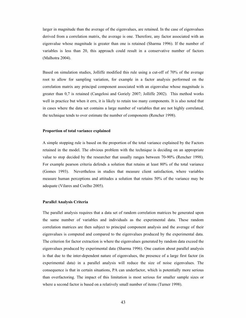
43
larger in magnitude than the average of the eigenvalues, are retained. In the case of eigenvalues
derived from a correlation matrix, the average is one. Therefore, any factor associated with an
eigenvalue whose magnitude is greater than one is retained (Sharma 1996). If the number of
variables is less than 20, this approach could result in a conservative number of factors
(Malhotra 2004).
Based on simulation studies, Jolliffe modified this rule using a cut-off of 70% of the average
root to allow for sampling variation, for example in a factor analysis performed on the
correlation matrix any principal component associated with an eigenvalue whose magnitude is
greater than 0,7 is retained (Cangelosi and Goriely 2007; Jolliffe 2002). This method works
well in practice but when it errs, it is likely to retain too many components. It is also noted that
in cases where the data set contains a large number of variables that are not highly correlated,
the technique tends to over estimate the number of components (Rencher 1998).
Proportion of total variance explained
A simple stopping rule is based on the proportion of the total variance explained by the Factors
retained in the model. The obvious problem with the technique is deciding on an appropriate
value to stop decided by the researcher that usually ranges between 70-90% (Rencher 1998).
For example pearson criteria defends a solution that retains at least 80% of the total variance
(Gomes 1993). Nevertheless in studies that measure client satisfaction, where variables
measure human perceptions and attitudes a solution that retains 50% of the variance may be
adequate (Vilares and Coelho 2005).
Parallel Analysis Criteria The parallel analysis requires that a data set of random correlation matrices be generated upon
the same number of variables and individuals as the experimental data. These random
correlation matrices are then subject to principal component analysis and the average of their
eigenvalues is computed and compared to the eigenvalues produced by the experimental data.
The criterion for factor extraction is where the eigenvalues generated by random data exceed the
eigenvalues produced by experimental data (Sharma 1996). One caution about parallel analysis
is that due to the inter-dependent nature of eigenvalues, the presence of a large first factor (in
experimental data) in a parallel analysis will reduce the size of noise eigenvalues. The
consequence is that in certain situations, PA can underfactor, which is potentially more serious
than overfactoring. The impact of this limitation is most serious for smaller sample sizes or
where a second factor is based on a relatively small number of items (Turner 1998).

44
It is, however, not necessary to run simulation studies described above for standardized data. A
regression equation has been developed to estimate eigenvalues for random data (Sharma 1996):
ln λk = ak + bk ln(n-1) + ck ln{(p-k-1)(p-k+2)/2}+ dk ln (λk-1) (3.3.27)
λk is the estimate for the kth eigenvalue, p is the number of variables, n is the number of
observations, ak,, bk , ck , dk are regression coefficients, and λ0 is assumed to be one (in appendix
B, the estimated regression coefficients using simulated data are displayed). Note from the
equation above that the two last eigenvalue values cannot be estimated because the third term
results in the logarithm of a zero or a negative value, which is undefined. Nevertheless the use
of simulation studies tends to produce better results and those will be used in this study.
3.3.8 Factor Solution Quality
Basically we want to assess how well can the factors account for the factor solution. The
residual correlation matrix can be used for this purpose. The residual correlation matrix gives
the amount of correlation that is not explained by the two factors, the diagonal contains the
unique variances and the off-diagonal elements contain the differences between observed
correlations and correlations explained by the estimated factor structure. Obviously, for a good
factor model the residual correlations should be as small as possible. The residual matrix can be
summarized by computing the square root of the average squared values of the off-diagonal
elements. This quantity, known as the root mean square residual (RMSR), should be small for a
good factor structure. The RMSR of the residual matrix is given by
2/)1(1 1
2
−=
∑ ∑= =
pp
resRMSR
p
i
p
j ij (3.3.28)
where resij is the correlation between the ith and jth variables and p is the number of variables
(Sharma 1996).

45
3.3.9 Factor Scores
As each factor is estimated as a linear combination of the original variables, for the observation
k, the score of the factor j is given by (Sharma 1996):
pkpjkjkjp
i ikijjk xwxwxwxwF +++==∑ =...22111
(3.3.29)
Where jkF is the estimated factor score for factor j for observation k, xik is the standardized
value of the variable i for the observation k, and wij is the factorial coefficient associated to the
variable i and the j. These scores can then be used in other analyses, such as the formation of
clusters, making it possible to classify individuals.
In Principal Component Analysis the scores are exact, but in Principal Axis Factoring they have
to be estimated (Vilares and Coelho 2005). There are four common methods to estimate factor
scores:
- Regression Scores: The factor scores are based on Z-scores and uses the matrix formula
(Z R-1 P = F), where Z is the Zscore matrix, R-1 is the inverse of the correlation matrix, P is the
pattern coefficient matrix, and F is the factor score matrix. The model assumes that the original
variables have a multivariate normal distribution (Johnson and Wichern 1998).
- Bartlett Scores: Uses least squares procedure to minimize the sum of squares of the unique
factors over the range of variables. Because the sum of squares of the unique factors are
minimized, non-common factors are used only to explain the discrepancies between observed
scores and those reproduced from the common factors. This method eventually leads to high
correlation between factor scores and factors being estimated (Bartlett 1937).
- Anderson-Rubin Scores: Proceed in the same manner as Bartlett except they added the
condition that the factor scores were required to be orthogonal, resulting in a more complex
equation than Bartlett’s. The Anderson-Rubin equation produces factor estimates whose
correlations form an identity matrix (Anderson and Rubin 1956).
However, these three (Regression, Bartlett, Anderson-Rubin) algorithms yield factor scores that
are in Zscore form (each set of factor scores has a mean of zero and a standard deviation of

46
one). The result does not allow comparison of the mean factor score on any given factor with
the mean on other factors for the same data set.
- Thompson Scores: Creates factor scores that are not generated in Zscore form and yields a
standardized, noncentered factor score, which allows comparisons of Fscore means. The
variables are converted to Zscore form then the original variable means are added back onto the
Zscores, so that the central tendency information is retrieved, then multiplied by the inverse of
the correlation matrix and by the pattern matrix as in the original regression algorithm.
Although, the standard deviation of the standardized factor scores is 1, like in Zscore based
formulas, the means of the measured variables are added back into factor scores (Thompson
1993).
Due to the factor indeterminacy problem a number of loading matrices are possible, each
resulting in a separate set of factor scores. In other words, the factor Scores are not unique. So
the factor scores to be used in other analysis should be the ones of the chosen solution.
3.3.10 Factor Analysis versus Principal Components Analysis
Although factor analysis and principal components analysis are typically labelled as data
reduction techniques, there are significant differences between the two techniques. The
objective of principal components analysis is to reduce the number of variables to few
components such that each component forms a new variable and the number of retained
components explains the maximum amount of variance in the data. The objective of factor
analysis, on the other hand, is to search or identify the underlying factor(s) or latent constructs
that can explain the intercorrelation among the variables. There are two major differences. First,
principal components analysis places emphasis on explaining the variance in the data, the
objective of factor analysis is to explain the correlation among the indicators. Second, in
principal components analysis the variables form an index. In factor analysis, on the other hand,
the variables or indicators reflect the presence of unobservable construct(s) or factor(s) (Sharma
1996).

47
3.3.11 Exploratory versus Confirmatory Factor Analysis
In an exploratory factor analysis the researcher has little or no knowledge about the factor
structure. In such a case, the researcher may collect data and explore or search for a factor
structure which can explain the correlations among the indicators. Such an analysis is called
exploratory factor analysis. Confirmatory factor analysis, on the other hand assumes that the
factor structure is known or hypothesized a priori. In other words, the complete factor structure
along with the respective indicators and the nature of pattern loadings is specified a priori. The
objective is to empirically verify or confirm the factor structure. Such an analysis is referred to
as confirmatory factor analysis (Sharma 1996).

48
3.4 HIERARCHICAL CLUSTERING ______________________________________________________________________
3.4.1 Introduction
Cluster analysis is used for classifying objects or cases, and sometimes variables, into relatively
homogeneous groups.
Hierarchical clustering is characterized by the development of a hierarchy or tree-like structure.
Hierarchical methods can be agglomerative or divisive. Agglomerative clustering starts with
each object in a separate cluster. Clusters are formed by grouping objects into bigger and bigger
clusters. This process is continued until all objects are members of a single cluster. Divisive
clustering starts with all the objects grouped in a single cluster. Clusters are divided or split until
each object is in separate cluster, this method is not commonly used and it’s computationally
demanding (Branco 2004; Malhotra 2004; Vilares and Coelho 2005).
3.4.2 Agglomerative Methods
Agglomerative methods are the most commonly used hierarchical methods. They consist of
linkage methods, error sums of squares or variance methods, and centroid methods (Malhotra
2004; Sharma 1996; Vilares and Coelho 2005).
Linkage methods are agglomerative methods of hierarchical clustering that cluster objects based
on a computation of the distance between them that include, single linkage, complete linkage,
and average linkage.
- Single linkage method: it’s based on minimum distance or the nearest neighbour rule. The
first two objects clustered are those that have the smallest distance between them. The next shortest distance is identified, and either the third object is clustered with the first two, or a, new
two-object cluster is formed. At every stage, the distance between two clusters is the distance
between their two closest points. Two clusters are merged at any stage by the single shortest
link between them. This process is continued until all objects are in one single cluster. The
single linkage method does not work well when the clusters are poorly defined (Branco 2004;
Malhotra 2004; Sharma 1996).
DAB = min {dij : i є A, j є B } (3.4.1)
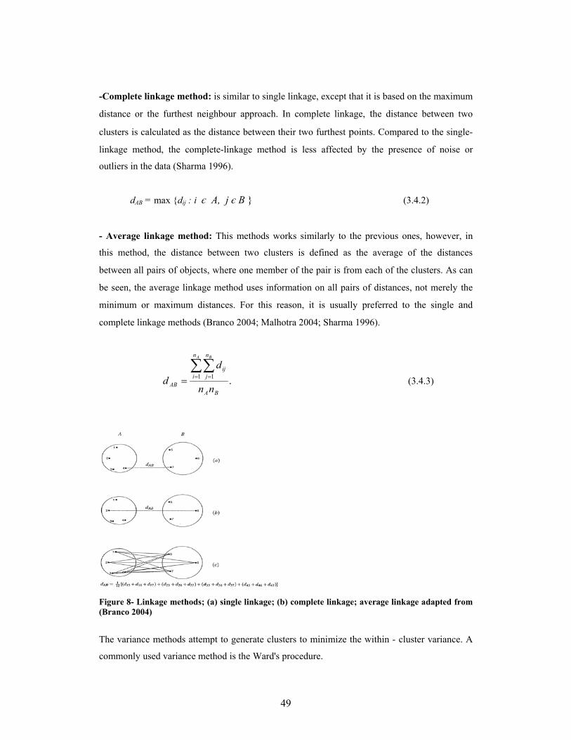
49
-Complete linkage method: is similar to single linkage, except that it is based on the maximum
distance or the furthest neighbour approach. In complete linkage, the distance between two
clusters is calculated as the distance between their two furthest points. Compared to the single-
linkage method, the complete-linkage method is less affected by the presence of noise or
outliers in the data (Sharma 1996).
dAB = max {dij : i є A, j є B } (3.4.2)
- Average linkage method: This methods works similarly to the previous ones, however, in
this method, the distance between two clusters is defined as the average of the distances
between all pairs of objects, where one member of the pair is from each of the clusters. As can
be seen, the average linkage method uses information on all pairs of distances, not merely the
minimum or maximum distances. For this reason, it is usually preferred to the single and
complete linkage methods (Branco 2004; Malhotra 2004; Sharma 1996).
.1 1
BA
n
i
n
jij
AB nn
dd
A B
∑∑= == (3.4.3)
Figure 8- Linkage methods; (a) single linkage; (b) complete linkage; average linkage adapted from (Branco 2004)
The variance methods attempt to generate clusters to minimize the within - cluster variance. A
commonly used variance method is the Ward's procedure.

50
- Ward's method: This, method does not compute distances between clusters. Rather, it forms
clusters by maximizing within-clusters homogeneity. The within-group (i.e., within-cluster) sum
of squares is used as the measure of homogeneity. That is, the Ward's method, tries to minimize
the total within-group or within-cluster sums of squares. Clusters are formed at each step such
that the resulting cluster solution has the fewest within-cluster sums of squares. The within-
cluster sums of squares that is minimized is also known as the error sums of squares (Sharma
1996).
SSWC − (SSWA + SSWB) (3.4.4)
Where
2
1
_
∑∑∈ =
⎟⎠⎞
⎜⎝⎛ −=
Ai
p
jjAijAA xxSSW
It’s the sum of squares within group A, 2
1
_
∑∑∈ =
⎟⎠⎞
⎜⎝⎛ −=
Ai
p
jjBijBB xxSSW
It’s the sum of squares within group B and 2
1
_
∑∑∈ =
⎟⎠⎞
⎜⎝⎛ −=
Ai
p
jjCijCC xxSSW
It’s the sum of squares within group C = A U B, that is the result of the agglutination of group A
with group B. ijAx ( ijBx ) it’s the observation of object i in group A and B in j variable, jAx_
and
jBx_
are the means of variable j in groups A and B.
- Centroid method: in this last method to be referred the distance between two clusters is the
distance between their centroids (means for a1l the variables). Every time objects are grouped, a
new centroid is computed (Johnson and Wichern 1998; Malhotra 2004;).
),(__
BAAB xxdd = (3.4.5)
Ax_
and Bx_
are the centroids of groups A and B.
A
Ai iA
nx
x ∑ ∈=_
and B
Bi iB
nx
x ∑ ∈=_
The centroid method is prone to the occurrence of inversions that is when an object joins an
existing cluster at a smaller distance than that of a previous consolidation, hence graphical

51
representations can be misleading, in all other four methods the dissimilarities are monotone.
Other methods exist but the ones above mentioned, are the more popular agglomerative
methods of hierarchical clustering (Malhotra 2004; Sharma 1996).
3.4.3 Distance Measures
The input for the clustering algorithm is the representation of the observations as a matrix of
similarity-dissimilarity. So it’s necessary to transform the original data to create these similarity
measures. These similarities – dissimilarities typically correspond to the distance between pairs
of objects. In fact all clustering algorithms require some type of measure or distance to asses the
similarity or dissimilarity of a pair of observations or clusters. The following distance measures
are considered to be the most commonly used in clustering (Sharma 1996; Vilares and Coelho
2005).
Distance measures between observations
The type of variables influence the distance measures used. There are distance measures for
quantitative variables and for qualitative variables (nominal and ordinal).
Quantitative Variables
In the case of quantitative variables the dissimilarity measure most known is the Euclidean
distance. In general the euclidean distance between points i and j in p dimensions is given by:
Euclidean Distance
( )2/1
1
2⎟⎟⎠
⎞⎜⎜⎝
⎛−= ∑
=
p
kjkikij XXD (3.4.6)
Where Dij is the distance between observations i and j, and p is the number of variables. It is
also common to use its square. The squared euclidean distance, as it follows above:

52
Squared Euclidean Distance
( )∑=
−=p
kjkikij XXD
1
22
(3.4.7)
Minkowski Distance
rp
k
r
jkikij xxD/1
1⎟⎟⎠
⎞⎜⎜⎝
⎛−= ∑
=
(3.4.8)
with r ≥ 1. If r =1 then we get city block distance, this measure is known by its robust behaviour
with outliers (Branco 2004). If r = 2 we get the Euclidean distance. Where Dij is the modulus of
the distance between observations i and j, and p is the number of variables.
Mahalanobis Distance
)()( 1/jijiij xxSxxD −−= − (3.4.9)
These dissimilarity distance, measures the distance between two observations i and j where S is
an estimation of the covariance matrix of the p variables. This measure accounts for the
correlation between variables and when S = I, Mahalonobis distance is equal to Euclidean
distance.
Qualitative Variables.
These types of variables will not be subject of analysis in this thesis but a brief description of
distance measures to be applied will be described. Of course when observations in a
multivariate sample are composed of qualitative nominal variables the distance metrics
mentioned above are not applicable, and association measures for crosstabs are used.
Obs j " 1 " " 0 "
Total
" 1 " a b a+b Obs i " 0 " c d c+d
Total a+c b+d p= a+b+c+d Table 4- Crosstabs with the values used for the association measures

53
Observations i and j are characterized by p- binary nominal variables where “1” and “0”, are the
presence or absence of the attribute. In this case a represents the number of attributes of the p
variables present in both individuals, b the number of attributes present in observation i but
absent in observation j, c represents the number of attributes absent in observation i, but present
in j and d represents the number of attributes absent in both observations.
Examples of common similarity coefficients:
Jacard
cbaasij ++
= (3.4.10)
Sorenson
cbaasij ++
=2
2 (3.4.11)
Russel & Rao
dcbaasij +++
= (3.4.12)
If the nominal variables have more than two levels the strategy is to transform each variable into
binary variables, as many, as the levels of the variable and proceed as above. In the case of
ordinal variables, we can decompose each variable in binary variables, but this procedure
despises the order, that is the propriety that distinguishes this type of variables from the
nominals. For example if the ordinal variable is the level of education of a person, we can
consider that a person has all the attributes related to the levels of education bellow the current
level (treat all the levels as binary levels, but consider 1 to current level and all levels bellow).
In a questionnaire with levels of satisfaction (very satisfied,…., unsatisfied) we can give a
ranking score and treat this variable as quantitative.
Proximity measures between variables
When the cluster analysis as the objective to group variables and not observations, the
appropriate similarity measures are the association and correlation coefficients (Branco 2004).

54
Quantitative Variables
The most commonly used for quantative variables is the Pearson Correlation,
∑ ∑
∑
= =
=
⎟⎠⎞
⎜⎝⎛ −⎟
⎠⎞
⎜⎝⎛ −
⎟⎠⎞
⎜⎝⎛ −⎟
⎠⎞
⎜⎝⎛ −
=n
K
n
K jkjiki
n
K jkjiki
ij
xxxx
xxxxr
1 1
2
.
_2
.
_
1 .
_
.
_
(3.4.13)
Qualitative Variables
For qualitative variables it is commonly used measures like Phi coefficient for nominal
variables and for ordinal variables the Spearman correlation (Vilares and Coelho 2005).
Phi Coefficient
Ф = (χ2/ n )1/2 where χ2 ∑∑= =
−=
r
i
s
j ji
jiij
fffff
n1 1 ..
2.. )(
(3.4.14)
But others like Cramer’s V can also be used for nominal variables.
)1(),1min(
2
−−Φ
=sr
V (3.4.15)
Spearman Correlation
=sr)1(
61 2
1
2
−−
∑=
nn
dn
kk
(3.4.16)
Where dk it’s the difference between the ranks that observation k takes in the variables i and j .

55
If the units are measured in vastly different units, the clustering solution will be influenced by
the units of measurement. In these cases, before clustering, we must standardize data by
rescaling each variable to have a mean of zero and a standard deviation of unity. Although
standardization can remove the influence of unit of measurement it can also reduce the
differences between groups on variables that may best discriminate groups or clusters (Malhotra
2004).
It is not uncommon to have data with variables of different types, different strategies can be
implemented, one is to transform quantitative variables into binary variables, another is to build
a combined similarity coefficient for observations i and j:
,321oij
nij
qijij swswsws ++= (3.4.17)
where qijs , n
ijs , oijs are the similarity coefficients, calculated for the quantitative, nominal and
ordinal variables and wk (k=1,2,3), are the weights.
A more elaborated formula of the combined similarity coefficient it’s presented (Gower 1971):
∑
∑
=
== p
kijk
p
kijkijk
ij
ss
1
1
ω
ω (3.4.18)
Where sijk it is the similarity between observations i and j in variable k. Generally ijkω takes
values one or zero in regard to the fact that the comparison of the observations i and j in variable
k is valid or not. Besides this ijkω is zero when the value in variable k is missed in at least one
of the observations i and j. When the variables are binary or nominal, sijk takes value one, if the
two objects have the same value in variable k and takes 0 if not. It is recommended for
continuous variables the use of the following similarity coefficient (Gower 1971):
k
jkikij r
xxs
−= (3.4.19)
Built based on the standardized city-block metric for variable k.

56
3.4.4 Techniques to decide the number of Clusters
A major issue in cluster analysis is to decide the number of clusters. Some of the most commons
techniques are explained (Sharma 1996):
- Theoretical, conceptual or practical considerations may suggest a certain number of clusters.
For example, if the purpose of clustering is to identify market segments, management may want
a particular number of clusters (Malhotra 2004).
- In hierarchical clustering the distances at which clusters are combined can be used as criteria.
This information can be obtained from the dendogram. In the dendogram bellow at the last two
stages, the clusters are being combined at large distances. Therefore in this example it appears
that a three-cluster solution is appropriate. For samples with a large number of observations this
method may not be more difficult to evaluate (Vilares and Coelho 2005).
Figure 9- Dendogram for hypothetical data
- Also using as criteria the distances at which clusters are combined, the agglomeration schedule
distances can be plotted against the number of clusters and the point when the slope decreases
reveals the number of clusters.
R2 Criteria
- Another common criteria, that can be used is the R- Squared. R2 is a measure of the percentage
of the total variance that it’s retained in each of the different cluster solutions that can be
obtained. It is the ratio between sum of the squares between cluster SSB and the sum of total
squares SST. R2 can be plotted against the number of clusters and the point at which an elbow or
a sharp bend occurs indicates an appropriate number of clusters.

57
∑
∑
=
=== g
kk
g
kk
g
SST
SSB
trTtrBR
1
12 (3.4.20)
∑∑∑= = =
⎟⎠⎞
⎜⎝⎛ −=
g
k
p
j
n
ijkji
k
xxtrT1 1 1
2_
..
_
2_
...
_
1 1⎟⎠⎞
⎜⎝⎛ −= ∑∑
= =jkj
g
k
p
jk xxntrB
with g groups of n1, n2, …… ng elements, where each observation is measured in a p dimensional
variable X(px1)
From the R 2 it is possible to obtain the semipartial R-squared (SPRSQ)
2
122
−−=Δ= gg RRRSPRSQ (3.4.21)
Cubic Clustering Criterion (CCC).
- A more complex criteria it’s the Cubic Clustering Criterion (CCC). CCC is obtained by
comparing the observed R2 to the approximate expected R2 using an approximate variance-
stabilizing transformation. Positive values of the CCC mean that the obtained R2 is greater than
would be expected if sampling from a uniform distribution in a hyperbox and therefore indicate
the possible presence of clusters. Treating the CCC as a standard normal test statistic provides a
crude test of the hypotheses. (Milligan and Cooper 1985):
the data has been sampled from a uniform distribution on a hyperbox (a p-
dimensional right parallelepiped).
the data has been sampled from a mixture of spherical multivariate normal
distributions with equal variances and equal sampling probabilities.
(3.4.22) Where:
p*= estimation of between-cluster dimension variation; n = number of groups in the solution;
E (R2)= expected R-Squared;
Peaks on the plot with the CCC greater than 2 or 3 indicate good clustering, peaks between 0
and 2 indicate possible clusters but should be interpreted cautiously. Very negative values of the

58
CCC, may be due to outliers. CCC is not an appropriate criterion for clusters that are highly
elongated or irregularly shaped (Milligan and Cooper 1985).
Mojena Criteria
- Also an effective selection rule is the Mojena Criteria. Milligan and Cooper (1985) revised the
initial criteria, because the initial one was not a stopping rule and proposed the following one:
jjj ksααα +=+
_
1 (3.4.23)
Where α1 ,α2,….. αj are the fusion coefficients and _
jα is the average and sαj the standard
deviation, the reference value for k in order to establish the number of cluster is 1,25.
Besides these criteria’s there are more. Milligan and Cooper (1985) compared more than 30
methods to determine the number of clusters. Nevertheless the most common criteria are
included in the discussion above.
3.4.5 Assess Reliability and Validity
Given the several judgments entailed in cluster analysis, no clustering solution should be
accepted without some assessment of its reliability and validity. The following procedures
provide adequate checks on the quality of clustering results (Branco 2004; Malhotra 2004).
- Perform cluster analysis on the same data using different distance measures. Compare the
results across measures to determine the stability of the solutions.
- Use different methods of clustering and compare the results.
- Split the data randomly into halves. Perform clustering separately on each half. Compare the
results between the two samples particularly compare cluster centroids across the two samp1es.
- In non-hierarchical clustering, the solution may depend on the order of the cases in the data
set. Make multiple runs using different order of cases until the solution stabilizes.
- When a natural structure in the data exist the dissimilarities between clusters became larger. A
measure of the magnitude of the existent structure is the agglomerative coefficient (AC). For

59
each observation i, m(i) is the dissimilarity between i and the first cluster in which i is
aggregated divided by the greatest level of fusion. The agglomerative coefficient is given by the
average of 1-m(i), i=1,…..,n:
( )( )
n
imAC
m
i∑
=
−= 1
1 (3.4.24)
If AC= 1, the groups are well separated and there is a natural structure in the data, in opposition
if AC=0, the observations make a unique group. AC has a propensity to increase with the
number of observations, what makes it a method not advisable to compare data structures with
large different sizes. Also when an outlier is included the AC usually increases, what should
take us to be careful when making an interpretation of a big AC (Branco 2004).
-The cophenetic correlation coefficient is an internal validation method that is the product
moment correlation between the distances in the proximity matrix and the cophenetic or
ultrametric distances in the solution. Values close to 1 indicate a solution of good quality, if the
value is bellow 0,8 we should question the existence of an hierarchical structure in the data and
consider using a non-hierarchical method. Also like in AC the presence of outliers should be
accounted when interpreting the result of cophenetic correlation coefficient (Branco 2004).
Cophenetic correlation coefficient is much more commonly used than AC.
- The Rand index or Rand measure is a measure of the similarity between two data clusters. It is
used for an external validation of the solution (Rand 1971).
Given a set of n elements S = {O1,…. On } and two partions of S to compare, X= {X1,…. Xr }
and, Y= {Y1,…. Ys } we define the following:
• a, the number of pairs of elements in S that are in the same set in X and in the same set in Y • b, the number of pairs of elements in S that are in different sets in X and in different sets in Y • c, the number of pairs of elements in S that are in the same set in X and in different sets in Y • d, the number of pairs of elements in S that are in different sets in X and in the same set in Y

60
The Rand index, R, is:
(3.4.25)
Intuitively, one can think of a + b as the number of agreements between X and Y and c + d as
the number of disagreements between X and Y. The Rand index has a value between 0 and 1,
with 0 indicating that the two data clusters do not agree on any pair of points and 1 indicating
that the data clusters are exactly the same.

61
3.5 SELF-ORGANIZING MAPS ______________________________________________________________________
3.5.1 Introduction
The Non Hierarchical Clustering methods are very useful to group large amount of data,
because they don’t need to calculate and store a new matrix of dissimilarity at each new step of
the algorithm Additionally the non hierarchical clustering methods are able to regroup the
individuals in a different cluster in which they were initially included, in opposition with the
Hierarchical Clustering methods were the inclusion of an individual in a cluster is definitive.
We can argue that the probability of a correct classification of an individual in a cluster is bigger
in the non hierarchical clustering.
There are other non hierarchical clustering methods, like k-means, fuzzy-set based clustering
algorithms and other partitioning clustering algorithms such as k-medoids, but the discussion of
these methods is beyond the scope of this work and they will not be used in this thesis, instead
this thesis will focus in using Self-Organizing Maps
Although the term “Self- Organizing Map”, could be applied to a number of different
approaches, we use it as a synonym of Kohonen’s Self organizing Map (Kohonen 2001), or
SOM for short, also known as Kohonen Neural Networks.
The basic idea of a SOM is to map the data patterns onto a n-dimensional grid of neurons or
units. That grid forms what is known as the output space, as opposed to the input space where
the data patterns are. This mapping tries to preserve the topological relations, i.e., patterns that
are close in the input space will be mapped to units that are close in the output space, and vice-
versa (Bação et al. 2005).
The output space will usually be 2-dimensional, and most of the implementation of SOM use a
rectangular grid of units. In order to provide even distances between the units in the output
space, hexagonal grids are sometimes used. Single-dimensional SOMs are also common, and
some authors have used 3-dimensional SOMs. Using higher SOMs, although posing no
theoretical difficulties is rare, since it is not possible to easy visualize the output space (Bação
2005).

62
There are two major ways of using the SOM, in clustering tasks. The first one consists on
building large SOMs, were each cluster can be represented by more than one unit (neuron). In
this case the U-Matrix is explored by the researcher to draw conclusions about the number and
nature of the clusters that are presented in the data.
The second approach consists on building small maps, were the number of units is much smaller
than the number of input vectors. In this case only one unit is supplied for each expected cluster.
This approach requires that the number of clusters be known in advance and is directly
comparable to k-means.
Each unit (neuron), being an input layer unit, has as many weights or coefficients as the input
patterns, and can be seen as a vector in the same space as patterns. When training or using a
SOM with a given input pattern, we calculate the distance between that pattern and every unit in
the network. We then select the unit that is closest as the winning unit, and say that the pattern is
mapped onto that unit. If the SOM as been trained with success, then patterns that are close in
the input space will be mapped to neurons that are close (or the same) in the output space. We
can say that SOM is topology preserving, in the sense that, as far as possible, neighborhoods are
preserved through the mapping process. (Bação 2005)
Before the training process, the units may be initialized randomly. Usually the training consists
on two parts (Kohonen 2001):
First: In this part of the training, also called the unfolding phase, the units are “spread out”, and
pulled towards the general area (in the input space).
Second: After the unfolding phase, the general shape of the network in the input space is
defined, and we can proceed to the second part of the training, that is the fine tuning phase,
where we will match the units as close as possible to the input patterns, thus decreasing the
quantization error.

63
3.5.2 Basic SOM Learning Algorithm:
The basic SOM training algorithm can be described as follows (Bação et al. 2004):
Let
W be a pxq grid of units wij where i and j are their coordinates on that grid.
X be the set of n training patterns x1, x2, .. xn
α be the learning rate assuming values in [0, 1], initialized to a given initial learning rate
r be the radius of the neighborhood function h (wij,, wmn,, r)
1 Repeat
2 For k=1 to n
3 For all wij ∈W, calculate dij = ││ xk - wij ││
4 Select the unit that minimizes dij as the winner wwinner
5 Update each unit wij ∈W: wij = wij + α h (wij,, wmn,, r) ││ xk - wij ││
6 Decreases the value of α and r
7 Until α reaches 0
This algorithm can be applied to a SOM with any dimension. The learning rate α, sometimes
referred to as η, must converge to 0 so as to guarantee convergence and stability to the SOM.
The decrease from the initial value of this parameter to zero is usually done linearly, but any
function may be used.
The neighborhood function, sometimes referred to as Λ or Nc, assumes values in [0,1], and is a
function of the position of two units (a winner unit, and another unit), and radius. It is large for
units that are close in the output space, and small (or 0) for units far away. Usually, it is a
function that as maximum at the center, monotonically decreases up to a radius r (also called the
neighborhood radius) and is zero from these onwards. The distance usually measured between
vectors it’s the Euclidean distance, but others can be used, like Minkowski distance, correlation,
Hausdorff distance etc…
3.5.3 Neighbourhood Functions
The two most common neighborhood functions are the Gaussian and the square (or bubble).
The update of both, the learning rate and the neighborhood radius, parameters may be done after
each training pattern is processed or after the whole training set is processed.

64
Gaussian
hg (wij,, wmn,) =
222 )()(
21
⎟⎟⎟
⎠
⎞
⎜⎜⎜
⎝
⎛ −+−−
rmjni
e
Square or Bubble
1 <= 22 )()( mjni −+− ≤ r
hg (wij,, wmn,) = 0 <= 22 )()( mjni −+− ≥ r
The algorithm is very robust in changes in the neighborhood function, and converges to final
maps very similarly. The Gaussian neighborhood function is usually more secure (all the
training sessions converge practically to the same map), and the bubble neighborhood function,
leads to less quantization errors (Kohonen 2001).
3.5.4 U- Matrix
There are several devices and techniques to visualize and explore the results of a SOM,
probably the most well- known output analysis tool is the U-Matrix. The U-Matrix constitutes a
representation of a SOM in which distances, in the input space, between neighboring units are
represented usually by a color code. If distances between neighboring units are small, then these
units represent a cluster of patterns of similar characteristics. If the units are far apart, then they
are located in a zone of the input space that has few patterns, and can be seen as a separation
between clusters. Distance can either be depicted as grey shades, or color ramps. Typically,
when using grey scales small distances between units are shown in white or light grey and big
distances in black or dark grey. In color ramps proximity is usually represented by deep blue
and large distances with dark red.
The development of the U-Matrix is fairly simple, first the distances between each pair of units
are calculated, this distance will be used to color the hexagons which separate the units. In a
second phase the distances calculated will be used to color the hexagons which represent the
units, leading to a U-Matrix which has the double (minus 1) of rows and columns of the initial
SOM (Bação 2005).

65
Figure 10- U-matrix
3.5.5 Component Planes
The basic idea is that each plane represents the value assumed by each neuron for each
component of the vector or variable. Thus, the color of each neuron represents the value of a
specific vector component. This method is useful to understand how the different variables that
compose the input vectors are organized in the SOM output space. Component planes analysis
can also be quite useful when searching for relations between variables (Bação 2005).
Figure 11- Component planes
3.5.6 SOM Quality
It is possible to measure the quality of the map using two different measures (Vesanto, Himberg
et al. 2000):
Average quantization error: This is simply the average distance from each data vector to
its best matching unit.
Topographic error: Gives the percentage of data vectors for which the best matching
unit and the second best matching are not neighboring map units.

66
3.5.7 Market Segmentation using Self- Organizing Maps
Market segmentation is above all a business need that emerges insides the companies and is
usually made inside the marketing departments or more recently by Customer Relationship
Management teams by organizations that already implemented this type of department or
structure.
Currently complex datamining software’s with large commercial implementation in the world
like SAS Enterprise Miner or Clementine already incorporate in their packages SOMs.
Nevertheless, for example, SAS Enterprise Miner approach is only based in the fact that the
number of clusters should be known in advance and is directly comparable to k-means in this
particularity, because in Enterprise Miner the visualization of the U-matrix is not incorporated
in the software, the researcher loses the possibility to draw conclusions about the number and
nature of the clusters that are presented in the data by doing the U-matrix analysis. Less
sophisticated and also less expensive statistical packages (like SPSS or SAS Enterprise Guide)
that are frequently used in market research usually only have the possibility to execute non-
hierarchical and k-means clustering methods, not being implemented in these software’s SOMs.
Even not being a so commonly used tool in market segmentation MatLab 7.0 with
SOM_TOOLBOX, enables the use of the U-matrix and a tighter control and a better definition
of the SOM algorithm parameters, and by these reasons was used in this thesis.
Self- Organizing Maps have been successfully applied as a classification tool to various
problems, including speech recognition, image or character recognition, applications in
geographical sciences and medical diagnosis but their use in market segmentations as a
clustering tool as been less used, nevertheless studies have been published using SOMs as a
clustering tool for market segmentation (Kiang et al 2002; Lien et al 2006; Rushmeir et al
1997). In commercial market research studies, the data tend to be markedly skewed, clearly
suggesting nonnormality and in these particular conditions SOMs demonstrated in some studies
to outperform k-means, being an useful and valid clustering tool for market segmentation
(Kiang et al 2002; Kiang et al 2006).

67
3.5.8 SOM Implementation in MATLAB
Due to the use o MATLAB in this thesis, a succinct description of the algorithm implementation
in MATLAB is described (Vesanto et al. 2000). The first step is to define all parameters needed
for the subsequent steps of the algorithm, which are summarized in Table 5. As there is no
theoretical definition of the optimal values for these initial parameters, user's experience and
knowledge is crucial on there definition and can be of greatest importance in the result of the
method.
The shape of the map is typically sheet type for its ease of visualization, but cylinder and toroid
shapes are also supported in MATLAB. Map lattice can be hexagonal or rectangular. The
initialization of the SOM units can be performed in two ways: linearly or in a random fashion. If a linear initialization is executed, the network is initially spread proportionally to the input
space. If a random initialization is selected, the units are set randomly in the input space. In this
case it means that most certainly the SOM will be folded in the beginning, but with correct
training parameters the unfolding is almost certain (Loureiro 2006).
Parameter name Parameter domain
Map Shape sheet; cylinder; toroid
Map lattice hexagonal; rectangular
Initialization type linear; random
Map size user dependent
Initial learning rate (α) user dependent, in [0,1]
Linear rate updating rule linear; power; inverse
Initial neighborhood radius (r) Gaussian; cut-Gaussian; bubble; epanechicov
Number of iterations user dependent
Number of training phases user dependent. If m more than one training phase is used, α, r, and number of iterations should be defined for each training phase.
Table 5- SOM parameters in SOM toolbox in MATLAB (Vesanto et al. 2000)
Map size is user dependent and the options have been already discussed above. The learning
rate α assumes values in [0,1] having an initial value α0 set by the user. It then decreases to zero
during the training phase, so as to guarantee convergence and stability for the SOM. In the
MATLAB implementation of SOM, the diminishing α value follows one of the three functions,
linear, power or inverse (Vesanto et al. 2000).
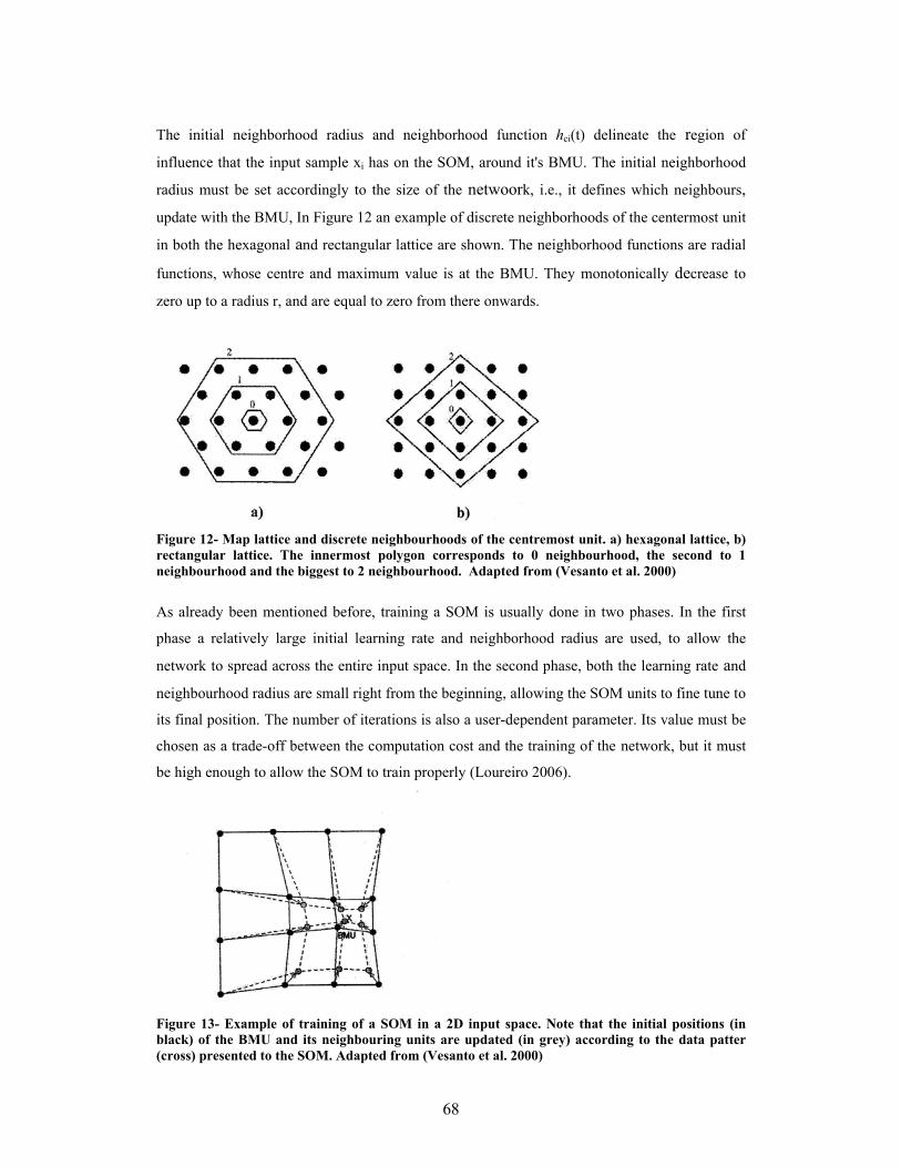
68
The initial neighborhood radius and neighborhood function hci(t) delineate the region of
influence that the input sample xi has on the SOM, around it's BMU. The initial neighborhood
radius must be set accordingly to the size of the netwoork, i.e., it defines which neighbours,
update with the BMU, In Figure 12 an example of discrete neighborhoods of the centermost unit
in both the hexagonal and rectangular lattice are shown. The neighborhood functions are radial
functions, whose centre and maximum value is at the BMU. They monotonically decrease to
zero up to a radius r, and are equal to zero from there onwards.
Figure 12- Map lattice and discrete neighbourhoods of the centremost unit. a) hexagonal lattice, b) rectangular lattice. The innermost polygon corresponds to 0 neighbourhood, the second to 1 neighbourhood and the biggest to 2 neighbourhood. Adapted from (Vesanto et al. 2000)
As already been mentioned before, training a SOM is usually done in two phases. In the first
phase a relatively large initial learning rate and neighborhood radius are used, to allow the
network to spread across the entire input space. In the second phase, both the learning rate and
neighbourhood radius are small right from the beginning, allowing the SOM units to fine tune to
its final position. The number of iterations is also a user-dependent parameter. Its value must be chosen as a trade-off between the computation cost and the training of the network, but it must
be high enough to allow the SOM to train properly (Loureiro 2006).
Figure 13- Example of training of a SOM in a 2D input space. Note that the initial positions (in black) of the BMU and its neighbouring units are updated (in grey) according to the data patter (cross) presented to the SOM. Adapted from (Vesanto et al. 2000)
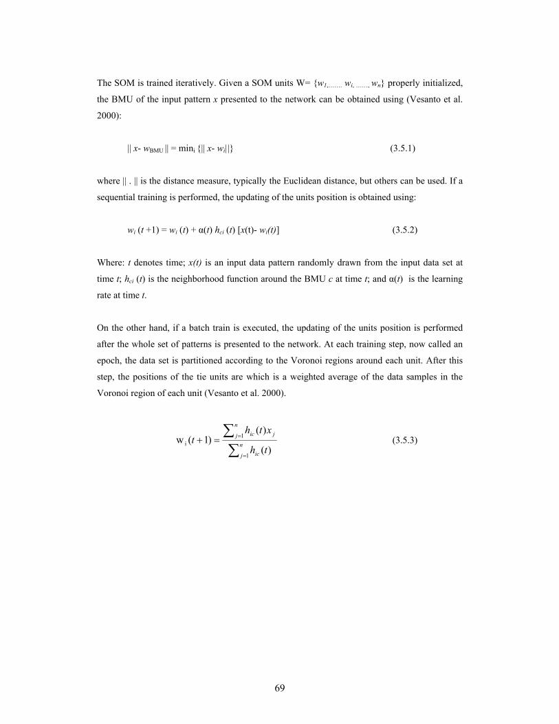
69
The SOM is trained iteratively. Given a SOM units W= {w1,……. wi, ……, wn} properly initialized,
the BMU of the input pattern x presented to the network can be obtained using (Vesanto et al.
2000):
|| x- wBMU || = mini {|| x- wi||} (3.5.1)
where || . || is the distance measure, typically the Euclidean distance, but others can be used. If a
sequential training is performed, the updating of the units position is obtained using:
wi (t +1) = wi (t) + α(t) hci (t) [x(t)- wi(t)] (3.5.2)
Where: t denotes time; x(t) is an input data pattern randomly drawn from the input data set at
time t; hci (t) is the neighborhood function around the BMU c at time t; and α(t) is the learning
rate at time t.
On the other hand, if a batch train is executed, the updating of the units position is performed
after the whole set of patterns is presented to the network. At each training step, now called an
epoch, the data set is partitioned according to the Voronoi regions around each unit. After this
step, the positions of the tie units are which is a weighted average of the data samples in the
Voronoi region of each unit (Vesanto et al. 2000).
∑
∑=
==+ n
j ic
n
j jic
th
xtht
1
1i
)(
)()1(w (3.5.3)

70
4. RESULTS ______________________________________________________________________
4.1. DESCRIPTIVE REPORTING ______________________________________________________________________
Most often customer databases in pharmaceutical industry are only subject to simple descriptive
statistical analysis and basic segmentations. It is important to start with a simple descriptive
statistical analysis of our data as a starting point for a next step multivariate statistical analysis,
but not to be strictly confined to descriptive statistics.
The database itself it is segmented by regions, aligned with the sales force distribution in the
field. An important absence in the file and in the CRM system in analysis is the absence of the
Customer Life Time Value that was not calculated. Sales information was given in the data file
in number of packs per product, in the original system this information is also in euros, but was
not made available for this study. All other variables used in the system for the company
Hospital business, were made available.
An annual patient treatment could range from 1-4 packs in all the products in the data file with
the exception of product F that it is only 1 pack per treatment per patient. Very often
management in the pharmaceutical industry likes to have analysis by regions, being these
regions aligned with the sales force distribution in order to check the performance of the
company in each of the regions and check the operational implementation of the sales and
marketing plans. Basically that’s why most of the pharmaceutical CRM programs in the
pharmaceutical industry are focused in SFA systems. The next table shows descriptive statistics
about the National results and different sales regions.

71
Region Total Calls Patients (anual)
Product B
Product A
Product C
Product D
Product F
Product E
Total Guideline
Mean 72,84 568,42 9,26 98 13,63 38,05 1,78 5,11 69,1Median 10 248 0 30 0 1 0 0 16Minimum 0 0 0 0 0 0 0 0 0Maximum 716 4745 169 850 116 808 35 86 530Std. Deviation 148,185 860,832 28,469 186,906 25,244 111,691 6,475 15,513 122,252
Total N=73 (100%)
Sum 5317 41495 676 7154 995 2778 130 373 5044
Mean 99,97 727,5 12,27 122,03 16,5 76,63 2,17 6,37 82,33Median 21,5 430 0 58 6,5 17 0 0 43Minimum 0 0 0 0 0 0 0 0 0Maximum 716 4745 150 800 83 808 35 82 436Std. Deviation 164,871 945,022 29,867 184,514 23,174 162,578 8,272 16,886 114,454Sum 2999 21825 368 3661 495 2299 65 191 2470
South N=30 (41,10%)
% of Total Sum 56,40% 52,60% 54,40% 51,20% 49,70% 82,80% 50,00% 51,20% 49,00%
Mean 41,78 300 0,65 42,78 7,74 1,09 0,87 5,39 42,26Median 0 42 0 0 0 0 0 0 0Minimum 0 0 0 0 0 0 0 0 0Maximum 525 1480 15 460 111 10 20 86 498Std. Deviation 116,685 464,049 3,128 101,338 24,443 2,678 4,17 18,364 110,638Sum 961 6900 15 984 178 25 20 124 972
Center N=23 (31,50%)
% of Total Sum 18,10% 16,60% 2,20% 13,80% 17,90% 0,90% 15,40% 33,20% 19,30%
Mean 67,85 638,5 14,65 125,45 16,1 22,7 2,25 2,9 80,1Median 11,5 282 0 31 1,5 2 0 0 27Minimum 0 0 0 0 0 0 0 0 0Maximum 610 3790 169 850 116 220 20 38 530Std. Deviation 153,632 1031,179 39,546 251,255 29,015 51,665 5,73 8,861 145,577Sum 1357 12770 293 2509 322 454 45 58 1602
North N=20 (27,4%)
% of Total Sum 25,50% 30,80% 43,30% 35,10% 32,40% 16,30% 34,60% 15,50% 31,80%
Table 6- Descriptive statistics per variable per region
Being all the products, drugs that are related with cancer patients, the variable patients that
measures the number of chemotherapy patients treated in 2004 is a good measure to access the
real potential of each region, ideally the proportion of product sales of each region should be
aligned with the region proportion of chemotherapy patients treated. Senior management
usually receives reports that show the deviation to the expected behaviour with highlights that
can be colours that like in the table above show in green the variables that are above or in line
with the expected performance, orange that are close to the expected performance, or red that in
this case are bellow 25% the expected performance in absolute value.
In the Center region, Product B and D performance are bellow expectations, in the case of
product D, this can be explained with the high proportion of sales of product E that is a

72
therapeutic equivalent to D. In the North region both product D and E are substantially bellow
the expected performance when compared with the proportion or percentage of chemotherapy
patients treated in this region. We can argue that the North might have a lower patient share in
product D and E, or the treatment approach in the North could be more conservative in the
number of packs they use to treat each patient, the same assumption can be draw to the Center
in respect to product B. In these cases the advice is to try to get more data that could help solve
these questions.
Ideally the company should have the right information per Hospital about the competitors
performance when a product have a therapeutically equivalent drug from other company, the
type of cancer tumours treated in each hospital and the number of patients treated per tumour in
each hospital, because the type of tumour is related with the type of treatment adoption and the
duration of the treatment, and with all these information it would be more easy to the company
to estimate the real number of patients treated with their pharmaceutical drugs. Because in
Europe and specifically in Portugal there are laws that limit the access to all these information,
very often we need to do assumptions with what we have available. Another important fact is
that very often epidemiological data is not immediately available and only in the beginning of
next year or even later is available, so it is not uncommon to start an analysis using sales data
from the current year with epidemiological data from last year, and update the analysis when the
epidemiological data from the year in analysis is made available.
Another very common type of analysis is to compare a target objective with actual performance.
Activity Performance
85%99%
121%
0500
100015002000250030003500
North Center South
num
ber
of c
alls
0%20%40%60%80%100%120%140%
Total Guideline Actual Calls % of Objective
Figure 14- Activity performance
In our case it seems that the total guideline that represents the number of target visits that the
sales representatives should do to the health professionals was not been accomplished in the
North in 2004. The calculation of the target visits or calls is made using internal empirical rules
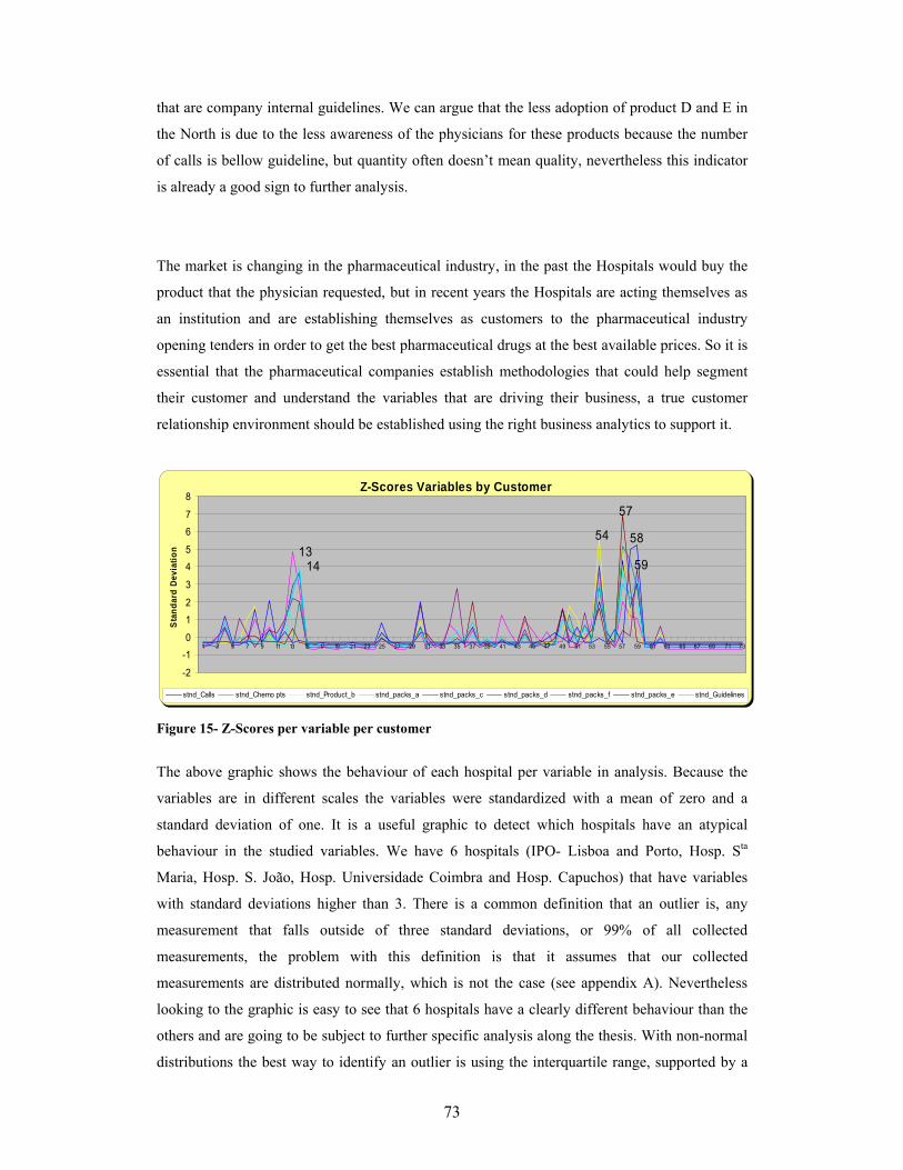
73
that are company internal guidelines. We can argue that the less adoption of product D and E in
the North is due to the less awareness of the physicians for these products because the number
of calls is bellow guideline, but quantity often doesn’t mean quality, nevertheless this indicator
is already a good sign to further analysis.
The market is changing in the pharmaceutical industry, in the past the Hospitals would buy the
product that the physician requested, but in recent years the Hospitals are acting themselves as
an institution and are establishing themselves as customers to the pharmaceutical industry
opening tenders in order to get the best pharmaceutical drugs at the best available prices. So it is
essential that the pharmaceutical companies establish methodologies that could help segment
their customer and understand the variables that are driving their business, a true customer
relationship environment should be established using the right business analytics to support it.
Z-Scores Variables by Customer
1354
14 59
57
58
-2
-1
0
1
2
3
4
5
6
7
8
1 3 5 7 9 11 13 15 17 19 21 23 25 27 29 31 33 35 37 39 41 43 45 47 49 51 53 55 57 59 61 63 65 67 69 71 73
Sta
ndar
d De
viat
ion
stnd_Calls stnd_Chemo pts stnd_Product_b stnd_packs_a stnd_packs_c stnd_packs_d stnd_packs_f stnd_packs_e stnd_Guidelines
Figure 15- Z-Scores per variable per customer
The above graphic shows the behaviour of each hospital per variable in analysis. Because the
variables are in different scales the variables were standardized with a mean of zero and a
standard deviation of one. It is a useful graphic to detect which hospitals have an atypical
behaviour in the studied variables. We have 6 hospitals (IPO- Lisboa and Porto, Hosp. Sta
Maria, Hosp. S. João, Hosp. Universidade Coimbra and Hosp. Capuchos) that have variables
with standard deviations higher than 3. There is a common definition that an outlier is, any
measurement that falls outside of three standard deviations, or 99% of all collected
measurements, the problem with this definition is that it assumes that our collected
measurements are distributed normally, which is not the case (see appendix A). Nevertheless
looking to the graphic is easy to see that 6 hospitals have a clearly different behaviour than the
others and are going to be subject to further specific analysis along the thesis. With non-normal
distributions the best way to identify an outlier is using the interquartile range, supported by a

74
graphical representation like the boxplot. These analysis were performed in appendix A and
these 6 hospitals appear all as extreme outliers in 3 variables (Total calls, Total Guideline,
Product A), and have a frequent outlier behaviour in other variables. Other hospitals have one or
another variable as an outlier but not as frequent as these 6. These 6 hospitals are obviously
extremely important customers for this pharmaceutical company (high positive z-scores) and
deserve a special treatment, they have common characteristics that were not included as a label
in the data file, the IPOs are Specialized Hospitals and the other four are Central Hospitals,
according to the Ministry of Health classifications in 2004. Two of them belong to the North
region (IPO Porto and S.João), one to the Center (Hosp. Universidade Coimbra) and three to the
South (Hosp. Capuchos, Hosp. Sta Maria, IPO- Lisboa).
Correlation Matrix(a)
Total Calls
Patients (anual)
Product B
Product A
Product C
Product D
Product F
Product E
Total Guideline
Total Calls 1 0,778 0,542 0,923 0,691 0,659 0,764 0,41 0,962Patients (anual) 0,778 1 0,539 0,831 0,681 0,445 0,519 0,242 0,815Product B 0,542 0,539 1 0,668 0,405 0,701 0,697 0,169 0,565Product A 0,923 0,831 0,668 1 0,707 0,628 0,795 0,303 0,941Product C 0,691 0,681 0,405 0,707 1 0,239 0,423 0,382 0,767Product D 0,659 0,445 0,701 0,628 0,239 1 0,754 0,181 0,569Product F 0,764 0,519 0,697 0,795 0,423 0,754 1 0,501 0,783Product E 0,41 0,242 0,169 0,303 0,382 0,181 0,501 1 0,485
Correlation
Total Guideline 0,962 0,815 0,565 0,941 0,767 0,569 0,783 0,485 1
Table 7- Correlation Matrix of the variables in analysis
Looking to the correlations between the variables in the analysis we can argue that most of the
variables have other variables that have high correlations between themselves, being the
exception, Product E, with more modest correlations. High correlations among the variables
indicate that the variables can be grouped in homogeneous sets of variables such that each set of
variables measures the same underlying constructs or dimensions.
Determinant = 6,405E-06

75
4.2. CHARACTERIZATION OF THE RELATIONSHIP BETWEEN BUSINESS ATTRIBUTES.
______________________________________________________________________
It is our aim to find relationships between the business variables in the company CRM dataset in
order to give evidence to the marketing department which variables correlate together and can
help driving the sales of the different products, and also to deploy multi-product sales force that
will promote products that share common business characteristics. Even being a relatively poor
data set that does not represent all the complexity of the pharmaceutical business, the
relationships that can be established between patient data, sales representatives activity data and
product sales data can be critical to improve the sales and marketing effectiveness of the
pharmaceutical company.
Factor analysis is an interdependence technique in which the whole set of interdependent
relationship is examined (Malhothra 2004). Particularly important in the Pharmaceutical
business as in other business area’s is to use techniques that can examine the relationships
among sets of interrelated variables, and that is why factor analysis is suitable for the purpose of
our study.
When using Principal Component Factoring (PCF) or Principal Axis Factoring (PAF) in
exploratory factor analysis as methods of extracting the factors from a set of data, no
distributional assumptions is needed, because none of our variables have a normal distribution
and no assumption was made on multivariate normality, makes these procedures as the ones to
be considered to be used in this study. PCF is generally preferred for purposes of data reduction,
while PAF is generally preferred when the research purpose is detecting data structure or casual
modelling. One of the objectives of factor analysis in this study is also to calculate factor scores
to be subsequently used in clustering techniques. Only in the case of principal component
factoring it is possible to compute exact factor scores. Moreover, in principal component
factoring these scores are uncorrelated, in PAF, estimates of these scores are obtained, and there
is no guarantee that the factors will be uncorrelated with each other. In most cases, there is very
little difference between the results of PCF and PAF, therefore in most of the cases it really does
not matter which of two techniques is used (Malhotra 2004; Sharma 1996). Both techniques will
be compared.
Because our variables are measured in different scales, it makes sense to use the correlation
matrix that is particularly important when we want to avoid those variables with a larger scale to
influence the structure of produced factors (Vilares and Coelho 2005).

76
Outliers can also influence the outcome of factor analysis. Single linkage clustering is a
hierarchical method that is very susceptible to the chaining effect and is affected by the presence
of outliers and by this reason can be used to detect the presence of them in multivariate data
(Branco 2004; Sharma 1996). Applying this method to our standardized data we detected the
atypical behaviour of the 6 hospitals mentioned before that by the observation of the dendogram
in appendix B we can easily cut the dendodrogram and see that we have 6 individual clusters
with these hospitals and one big cluster with all the other observations.
The following factor analysis includes all the observations, the comments about the correlation
matrix have been already mentioned in the descriptive statistics section.
KMO and Bartlett's Test
,784
815,16336
,000
Kaiser-Meyer-Olkin Measure of SamplingAdequacy.
Approx. Chi-SquaredfSig.
Bartlett's Test ofSphericity
Table 8- Factor Analysis KMO and Bartlett’s Test for all the observations
The table 8 shows two tests which indicate the suitability of our data for factor analysis. The
KMO value indicates a middling appropriateness for factor analysis close to meritorious. The
null hypothesis that the population correlation matrix is an identity matrix, is rejected by the
Bartlett’s test of sphericity. An orthogonal correlation matrix will have a determinant of one,
indicating that the variables are not correlated. On the other hand, if there is a perfect correlation
between two or more variables the determinant will be zero, and the correlation matrix cannot
be inverted, and certain factor extraction methods will be impossible to compute, our correlation
matrix determinant is low but is different from zero. Overall, though, it appears that our data is
appropriate for factoring.
The reason why we didn’t removed the 6 Hospitals identified as outliers by the single linkage
method is that their removal led to a decrease in the KMO value to the range of mediocreness as
seen in table 9.
KMO and Bartlett's Test
,679
401,74336
,000
Kaiser-Meyer-Olkin Measure of SamplingAdequacy.
Approx. Chi-SquaredfSig.
Bartlett's Test ofSphericity
Table 9- Factor Analysis KMO and Bartlett’s Test excluding outliers

77
Also an immediate consequence of the removal of these 6 observations led to a KMO value of
0,340 for Product F indicating that the variable doesn’t seem to fit with the structure of the other
variables when these 6 hospitals are removed. If we make another extraction after removing
Product F, Product B KMO reduced to 0,407. We can conclude that by removing these hospitals
from the analysis, two variables doesn’t seem to fit with the structure of the other variables,
demonstrating that a blind removal of atypical values from factor analysis leads to loss of
interpretability and quality in the factor solution provided by these observations (in appendix B
all the KMO values are provided).
Anti-image Matrices
3,960E-02 1,571E-02 3,428E-02 -1,04E-02 1,637E-02 -5,51E-02 2,019E-02 -1,51E-03 -2,245E-021,571E-02 ,208 -4,30E-02 -3,75E-02 2,913E-02 -3,08E-02 7,254E-02 -3,09E-02 -2,158E-023,428E-02 -4,30E-02 ,295 -2,77E-02 -6,42E-02 -,108 -3,66E-02 1,579E-02 1,246E-03
-1,042E-02 -3,75E-02 -2,77E-02 4,828E-02 -1,80E-02 2,139E-02 -3,21E-02 7,736E-02 -8,393E-031,637E-02 2,913E-02 -6,42E-02 -1,80E-02 ,275 1,297E-02 7,104E-02 -6,43E-02 -3,149E-02
-5,511E-02 -3,08E-02 -,108 2,139E-02 1,297E-02 ,204 -6,69E-02 5,255E-02 2,631E-022,019E-02 7,254E-02 -3,66E-02 -3,21E-02 7,104E-02 -6,69E-02 ,103 -9,77E-02 -1,819E-02
-1,509E-03 -3,09E-02 1,579E-02 7,736E-02 -6,43E-02 5,255E-02 -9,77E-02 ,397 -2,629E-02-2,245E-02 -2,16E-02 1,246E-03 -8,39E-03 -3,15E-02 2,631E-02 -1,82E-02 -2,63E-02 2,415E-02
,781a ,173 ,317 -,238 ,157 -,614 ,316 -1,20E-02 -,726,173 ,847a -,173 -,374 ,122 -,150 ,495 -,107 -,304,317 -,173 ,841a -,232 -,225 -,441 -,210 4,610E-02 1,475E-02
-,238 -,374 -,232 ,833a -,156 ,216 -,456 ,559 -,246,157 ,122 -,225 -,156 ,842a 5,482E-02 ,423 -,195 -,386
-,614 -,150 -,441 ,216 5,482E-02 ,708a -,462 ,185 ,375,316 ,495 -,210 -,456 ,423 -,462 ,725a -,483 -,365
-1,203E-02 -,107 4,610E-02 ,559 -,195 ,185 -,483 ,590a -,268-,726 -,304 1,475E-02 -,246 -,386 ,375 -,365 -,268 ,795a
Total CallsPatients (anual)Product BProduct AProduct CProduct DProduct FProduct ETotal GuidelineTotal CallsPatients (anual)Product BProduct AProduct CProduct DProduct FProduct ETotal Guideline
Anti-image Covariance
Anti-image Correlation
Total CallsPatients(anual) Product B Product A Product C Product D Product F Product E
TotalGuideline
Measures of Sampling Adequacy(MSA)a.
Table 10- PCF Factor Analysis Anti- image Matrices for all the observations
A very important result is given by the diagonal elements on the anti-image correlation matrix
that are the KMO individual statistics for each variable. Values less than 0,5 may indicate
variables that do not seem to fit with the structure of the other variables and we should consider
dropping such variables from your analysis (Malhotra 2004), what is not the case in any of the
variables in this study.
Total Variance Explained
5,954 66,160 66,1601,124 12,488 78,647
,902 10,019 88,667,413 4,594 93,260,260 2,892 96,152,211 2,343 98,495
8,532E-02 ,948 99,4433,404E-02 ,378 99,8211,611E-02 ,179 100,000
Component123456789
Total % of Variance Cumulative %Initial Eigenvalues
Extraction Method: Principal Component Analysis. Table 11 - PCF Factor Analysis Anti- image Matrices for all the observations

78
How many factors should we extract? According to Kaiser Rule we should drop all components
or factors with eigenvalues under 1.0, keeping two factors. Another example is the pearson
criteria that defends a solution that retains at least 80% of the total variance, being in this case a
solution of three factors. Jolliffe's Rule defends that a factor analysis performed on the
correlation matrix any principal component or factor associated with an eigenvalue whose
magnitude is greater than 0,7 is retained to allow for sampling variation, being in this case again
a solution of three factors.
A very common criterion like Kaiser Rule is the Scree test:
Scree Plot
0
1
2
3
4
5
6
7
1 2 3 4 5 6 7 8
Factor Number
Eige
nval
ue
Figure 16- Factor analysis scree plot
The Cattel scree test above indicates a possible solution of two factors. Another method that
also relies in graphical representation is parallel analysis but with a defined criterion for factor
extraction that is where the eigenvalues generated by random data exceed the eigenvalues
produced by experimental data, which can be graphical visualised by the location where the two
lines of eigenvalues values intersect.
Parallel Analysis
0
1
2
3
4
5
6
7
1 2 3 4 5 6 7 8Factor Number
Eige
nval
ue
Random Eigenvalues Experimental Eigenvalues
Figure 17- Factor analysis Parallel analysis

79
A first observation might indicate a solution of two factors, but if we are really strict to the rule,
only one factor should be extracted. Parallel analysis is usually known as a very good method
(Sharma 1996), but one caution about parallel analysis should be taken and is due to the inter-
dependent nature of eigenvalues, the presence of a large first factor (in experimental data)
particularly in small samples can lead in certain situations that parallel analysis can underfactor,
which is potentially more serious than overfactoring (Turner 1998), and this is the case in our
experimental data. In appendix B an explanation of how the calculation of the random
eigenvalues was done is provided.
So we have methods that indicate a possible two factor solution or three factor solution.
Particularly in our study where a business solution is required, interpretability should be one of
the most important criteria in determining the number of factors (Vilares and Coelho 2005), and
will be the decisive criteria to decide the appropriate number of factors, between a solution of
two or three.
Table 12 - Factor analysis Communalities for PCF two factors extraction method All variables have high communality in the PCF extraction for two factors, with the exception
of Product E, when a communality of a variable is low there is the possibility to remove the
variable from the model, but what is really critical is not the communality coefficient per se, but
rather the extent to which the item is contributing to a well defined factor, though often this role
is greater when communality is high.
Total Variance Explained
5,954 66,160 66,160 3,587 39,852 39,8521,124 12,488 78,647 3,492 38,795 78,647
Component12
Total % of Variance Cumulative % Total % of Variance Cumulative %Extraction Sums of Squared Loadings Rotation Sums of Squared Loadings
Extraction Method: Principal Component Analysis. Table 13- PCF Factor Analysis Eigenvalues for two factor extraction
Communalities
1,000 ,8981,000 ,7141,000 ,7541,000 ,9171,000 ,7811,000 ,8611,000 ,8041,000 ,3881,000 ,961
Total CallsPatients (anual)Product BProduct AProduct CProduct DProduct FProduct ETotal Guideline
Initial Extraction
Extraction Method: Principal Component Analysis.

80
Component Matrix a
,943 8,796E-02,825 ,184,730 -,469,957 1,260E-02,734 ,492,718 -,588,860 -,256,466 ,414,962 ,192
Total CallsPatients (anual)Product BProduct AProduct CProduct DProduct FProduct ETotal Guideline
1 2Component
Extraction Method: Principal Component Analysis.2 components extracted.a.
Table 14- PCF Factor Matrix for two factor extraction This table reports the factor loadings for each variable on the unrotated components or factors.
High loadings of a variable on a factor indicate that there is much in common between the factor
and the respective variable. It has been suggested that a loading should be consider high if it is
at least greater than 0,6 (Sharma 1996), although some researchers consider cutoff valus as low
as 0,4 (Sharma 1996), we will aim for 0,6 during this study. By examining table 14, none of the
variables load highly in the second factor, but we can argue that there is a clear pattern to the
signs of the loadings in the second factor. Loadings of Products, B, D and F have a negative
sign that implies a different behaviour compared to the other variables. In contrast to the other
variables Product E does not have high loadings in none of the factors.
In sales and marketing when we want to implement a strategy or to send out a message, it
should be meaningful and very objective. So it makes sense to apply a factor rotation to achieve
a simpler and more meaningful factor structure. The objective of varimax rotation is such that
any given factor will have some variables that will load very high on it and some that will load
very low on it. A varimax solution yields results which make it as easy as possible to identify
each variable with a single factor, what makes it suitable as an ideal method to implement
directed sales and marketing strategies to sets of Factors represented by specific variables.
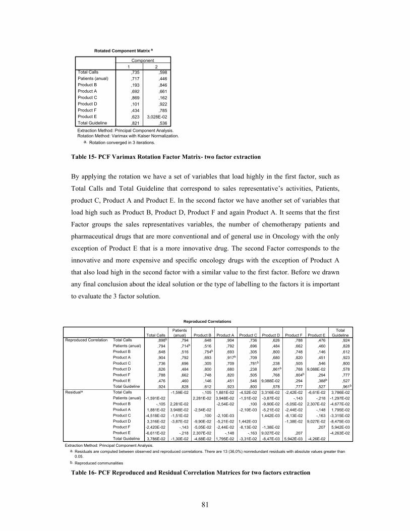
81
Rotated Component Matrix a
,735 ,598,717 ,446,193 ,846,692 ,661,869 ,162,101 ,922,434 ,785,623 3,028E-02,821 ,536
Total CallsPatients (anual)Product BProduct AProduct CProduct DProduct FProduct ETotal Guideline
1 2Component
Extraction Method: Principal Component Analysis. Rotation Method: Varimax with Kaiser Normalization.
Rotation converged in 3 iterations.a.
Table 15- PCF Varimax Rotation Factor Matrix- two factor extraction
By applying the rotation we have a set of variables that load highly in the first factor, such as
Total Calls and Total Guideline that correspond to sales representative’s activities, Patients,
product C, Product A and Product E. In the second factor we have another set of variables that
load high such as Product B, Product D, Product F and again Product A. It seems that the first
Factor groups the sales representatives variables, the number of chemotherapy patients and
pharmaceutical drugs that are more conventional and of general use in Oncology with the only
exception of Product E that is a more innovative drug. The second Factor corresponds to the
innovative and more expensive and specific oncology drugs with the exception of Product A
that also load high in the second factor with a similar value to the first factor. Before we drawn
any final conclusion about the ideal solution or the type of labelling to the factors it is important
to evaluate the 3 factor solution.
Reproduced Correlations
,898b ,794 ,648 ,904 ,736 ,626 ,788 ,476 ,924,794 ,714b ,516 ,792 ,696 ,484 ,662 ,460 ,828,648 ,516 ,754b ,693 ,305 ,800 ,748 ,146 ,612,904 ,792 ,693 ,917b ,709 ,680 ,820 ,451 ,923,736 ,696 ,305 ,709 ,781b ,238 ,505 ,546 ,800,626 ,484 ,800 ,680 ,238 ,861b ,768 9,088E-02 ,578,788 ,662 ,748 ,820 ,505 ,768 ,804b ,294 ,777,476 ,460 ,146 ,451 ,546 9,088E-02 ,294 ,388b ,527,924 ,828 ,612 ,923 ,800 ,578 ,777 ,527 ,961b
-1,59E-02 -,105 1,881E-02 -4,52E-02 3,316E-02 -2,42E-02 -6,61E-02 3,786E-02-1,591E-02 2,281E-02 3,948E-02 -1,51E-02 -3,87E-02 -,143 -,218 -1,297E-02
-,105 2,281E-02 -2,54E-02 ,100 -9,90E-02 -5,05E-02 2,307E-02 -4,677E-021,881E-02 3,948E-02 -2,54E-02 -2,10E-03 -5,21E-02 -2,44E-02 -,148 1,795E-02
-4,518E-02 -1,51E-02 ,100 -2,10E-03 1,442E-03 -8,13E-02 -,163 -3,315E-023,316E-02 -3,87E-02 -9,90E-02 -5,21E-02 1,442E-03 -1,38E-02 9,027E-02 -8,475E-03
-2,420E-02 -,143 -5,05E-02 -2,44E-02 -8,13E-02 -1,38E-02 ,207 5,942E-03-6,611E-02 -,218 2,307E-02 -,148 -,163 9,027E-02 ,207 -4,263E-023,786E-02 -1,30E-02 -4,68E-02 1,795E-02 -3,31E-02 -8,47E-03 5,942E-03 -4,26E-02
Total CallsPatients (anual)Product BProduct AProduct CProduct DProduct FProduct ETotal GuidelineTotal CallsPatients (anual)Product BProduct AProduct CProduct DProduct FProduct ETotal Guideline
Reproduced Correlation
Residuala
Total CallsPatients(anual) Product B Product A Product C Product D Product F Product E
TotalGuideline
Extraction Method: Principal Component Analysis.Residuals are computed between observed and reproduced correlations. There are 13 (36,0%) nonredundant residuals with absolute values greater than0.05.
a.
Reproduced communalitiesb.
Table 16- PCF Reproduced and Residual Correlation Matrices for two factors extraction

82
Instead of calculating RMSR, SPSS indicates how many residual correlations (bellow the
diagonal of the residual matrix) are above 0,05. It should be noted that there are no hard and fast
rules regarding how many should be less than 0,05 for a good factor solution (Sharma 1996) ,
though 36% of nonredundant residuals with values greater 0,05 could be regarded as an
acceptable solution. Nevertheless it is possible and is very important for accessing the quality of
the solution to use table 16 to compute the square root of the average squared values of the off-
diagonal elements or RMSR (Sharma 1996). The RMSR in this case is 0,067. A good indicator
for a good factor solution is an RMSR inferior to 0,1 (Sharma 1996). The RMSR is also a good
measure to compare the quality of different factor solutions.
Communalities
1,000 ,9001,000 ,8411,000 ,7561,000 ,9461,000 ,8271,000 ,8751,000 ,9121,000 ,9621,000 ,962
Total CallsPatients (anual)Product BProduct AProduct CProduct DProduct FProduct ETotal Guideline
Initial Extraction
Extraction Method: Principal Component Analysis. Table 17- Factor analysis Communalities for PCF three factors extraction method
All variables have high communality in the PCF extraction for three factors, including Product
E, showing the importance of the third factor in the communality of this variable.
Total Variance Explained
5,954 66,160 66,160 3,656 40,617 40,6171,124 12,488 78,647 2,991 33,238 73,855,902 10,019 88,667 1,333 14,811 88,667
Component123
Total % of Variance Cumulative % Total % of Variance Cumulative %Extraction Sums of Squared Loadings Rotation Sums of Squared Loadings
Extraction Method: Principal Component Analysis. Table 18- PCF Factor Analysis Eigenvalues for three factor extraction The extracted eigenvalue for the third component or factor is close to one but after Factor
Rotation the third value is now higher than one indicating that the rotation significantly
impacted the variance accounted by the third factor or component (particularly if we think about
the rationale behind the eigenvalue greater than one rule, that for standardized data the amount
of variance extracted by each component, should at a minimum, be equal to the variance of at
least one variable).

83
Component Matrixa
,943 8,796E-02 -4,78E-02,825 ,184 -,358,730 -,469 -4,52E-02,957 1,260E-02 -,171,734 ,492 -,214,718 -,588 ,117,860 -,256 ,327,466 ,414 ,757,962 ,192 -2,59E-02
Total CallsPatients (anual)Product BProduct AProduct CProduct DProduct FProduct ETotal Guideline
1 2 3Component
Extraction Method: Principal Component Analysis.3 components extracted.a.
Table 19- PCF Factor Matrix for three factor extraction
By examining table 19, none of the variables load highly in the second factor, but we can argue
that there is a clear pattern to the signs of the loadings in the second factor equal to the previous
unrotated two factors or components extraction. Product E as expected load highly in third
component or factor.
Table 20- PCF Varimax Rotation Factor Matrix for three factor extraction By applying the rotation we have a set of variables that load highly in the first factor, such as
Total Calls and Total Guideline that correspond to sales representative’s activities, Patients,
product C, Product A. In the second factor we have another set of variables that load high such
as Product B, Product D and Product F. Product E loads very high in the third factor.
Nevertheless only after PAF extraction and validation of the final solution we will provide the
labelling for the factors.
Rotated Component Matrixa
,756 ,513 ,258,861 ,317 -6,54E-03,321 ,807 -2,50E-02,786 ,560 ,124,881 4,615E-02 ,218,177 ,916 6,506E-02,348 ,783 ,422,194 9,061E-02 ,957,810 ,448 ,324
Total CallsPatients (anual)Product BProduct AProduct CProduct DProduct FProduct ETotal Guideline
1 2 3Component
Extraction Method: Principal Component Analysis. Rotation Method: Varimax with Kaiser Normalization.
Rotation converged in 5 iterations.a.
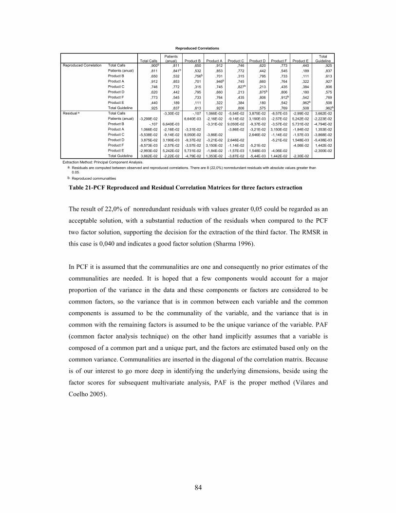
84
Reproduced Correlations
,900b ,811 ,650 ,912 ,746 ,620 ,773 ,440 ,925,811 ,841b ,532 ,853 ,772 ,442 ,545 ,189 ,837,650 ,532 ,756b ,701 ,315 ,795 ,733 ,111 ,613,912 ,853 ,701 ,946b ,745 ,660 ,764 ,322 ,927,746 ,772 ,315 ,745 ,827b ,213 ,435 ,384 ,806,620 ,442 ,795 ,660 ,213 ,875b ,806 ,180 ,575,773 ,545 ,733 ,764 ,435 ,806 ,912b ,542 ,769,440 ,189 ,111 ,322 ,384 ,180 ,542 ,962b ,508,925 ,837 ,613 ,927 ,806 ,575 ,769 ,508 ,962b
-3,30E-02 -,107 1,066E-02 -5,54E-02 3,875E-02 -8,57E-03 -2,99E-02 3,662E-02-3,299E-02 6,640E-03 -2,16E-02 -9,14E-02 3,190E-03 -2,57E-02 5,242E-02 -2,223E-02
-,107 6,640E-03 -3,31E-02 9,050E-02 -9,37E-02 -3,57E-02 5,731E-02 -4,794E-021,066E-02 -2,16E-02 -3,31E-02 -3,86E-02 -3,21E-02 3,150E-02 -1,84E-02 1,353E-02
-5,538E-02 -9,14E-02 9,050E-02 -3,86E-02 2,646E-02 -1,14E-02 -1,57E-03 -3,868E-023,875E-02 3,190E-03 -9,37E-02 -3,21E-02 2,646E-02 -5,21E-02 1,548E-03 -5,438E-03
-8,573E-03 -2,57E-02 -3,57E-02 3,150E-02 -1,14E-02 -5,21E-02 -4,06E-02 1,442E-02-2,993E-02 5,242E-02 5,731E-02 -1,84E-02 -1,57E-03 1,548E-03 -4,06E-02 -2,300E-023,662E-02 -2,22E-02 -4,79E-02 1,353E-02 -3,87E-02 -5,44E-03 1,442E-02 -2,30E-02
Total CallsPatients (anual)Product BProduct AProduct CProduct DProduct FProduct ETotal GuidelineTotal CallsPatients (anual)Product BProduct AProduct CProduct DProduct FProduct ETotal Guideline
Reproduced Correlation
Residual a
Total CallsPatients(anual) Product B Product A Product C Product D Product F Product E
TotalGuideline
Extraction Method: Principal Component Analysis.Residuals are computed between observed and reproduced correlations. There are 8 (22,0%) nonredundant residuals with absolute values greater than0.05.
a.
Reproduced communalitiesb.
Table 21-PCF Reproduced and Residual Correlation Matrices for three factors extraction
The result of 22,0% of nonredundant residuals with values greater 0,05 could be regarded as an
acceptable solution, with a substantial reduction of the residuals when compared to the PCF
two factor solution, supporting the decision for the extraction of the third factor. The RMSR in
this case is 0,040 and indicates a good factor solution (Sharma 1996).
In PCF it is assumed that the communalities are one and consequently no prior estimates of the
communalities are needed. It is hoped that a few components would account for a major
proportion of the variance in the data and these components or factors are considered to be
common factors, so the variance that is in common between each variable and the common
components is assumed to be the communality of the variable, and the variance that is in
common with the remaining factors is assumed to be the unique variance of the variable. PAF
(common factor analysis technique) on the other hand implicitly assumes that a variable is
composed of a common part and a unique part, and the factors are estimated based only on the
common variance. Communalities are inserted in the diagonal of the correlation matrix. Because
is of our interest to go more deep in identifying the underlying dimensions, beside using the
factor scores for subsequent multivariate analysis, PAF is the proper method (Vilares and
Coelho 2005).

85
Communalities
,960 ,903,792 ,685,705 ,606,952 ,928,725 ,695,796 ,803,897 ,820,603 ,183,976 ,995
Total CallsPatients (anual)Product BProduct AProduct CProduct DProduct FProduct ETotal Guideline
Initial Extraction
Extraction Method: Principal Axis Factoring. Table 22- Factor analysis Communalities for PAF two factors extraction method The final communalities are the communalities of the last iteration. Again product E has a low
communality.
Total Variance Explained
5,954 66,160 66,160 5,770 64,114 64,114 3,766 41,844 41,8441,124 12,488 78,647 ,847 9,416 73,531 2,852 31,686 73,531
,902 10,019 88,667,413 4,594 93,260,260 2,892 96,152,211 2,343 98,495
8,532E-02 ,948 99,4433,404E-02 ,378 99,8211,611E-02 ,179 100,000
Factor123456789
Total % of Variance Cumulative % Total % of Variance Cumulative % Total % of Variance Cumulative %Initial Eigenvalues Extraction Sums of Squared Loadings Rotation Sums of Squared Loadings
Extraction Method: Principal Axis Factoring. Table 23- Factor analysis Communalities for PAF two factors extraction method In PAF extraction the eigenvalues after extraction will be lower than their initial counterparts,
because these are these eigenvalues that result from the modified correlation matrix where the
diagonals contain the estimated communalities (Sharma 1996).
Factor Matrixa
,945 -,101,796 -,226,696 ,348,961 -6,27E-02,707 -,441,705 ,554,848 ,319,412 -,112,974 -,215
Total CallsPatients (anual)Product BProduct AProduct CProduct DProduct FProduct ETotal Guideline
1 2Factor
Extraction Method: Principal Axis Factoring.Attempted to extract 2 factors. More than 2iterations required. (Convergence=4,915E-02).Extraction was terminated.
a.
Table 24- PAF Factor Matrix for two factor extraction It was not possible to make more than two iterations because at the third iteration the
communality of a variable exceeded one. By examining table 24, none of the variables load
highly in the second factor, but we can argue that there is a clear pattern to the signs of the
loadings in the second factor identical to the PCF extraction. Again in contrast to the other
variables Product E does not have high loadings in none of the factors.

86
Rotated Factor Matrix a
,792 ,525,757 ,334,314 ,712,780 ,565,826 ,111,189 ,876,449 ,786,389 ,177,887 ,456
Total CallsPatients (anual)Product BProduct AProduct CProduct DProduct FProduct ETotal Guideline
1 2Factor
Extraction Method: Principal Axis Factoring. Rotation Method: Varimax with Kaiser Normalization.
Rotation converged in 3 iterations.a.
Table 25-PAF Varimax Rotation Factor Matrix- two factor extraction The rotated factor structure in PAF extraction gives the same interpretation like the PCF two
factors extraction with the exception of product E that in PAF doesn’t load high in any of the
factors structures. Because the KMO of variable E is not low enough so that we should consider
immediately dropping this variable from our analysis, a third factor must be extracted. PAF
clearly indicates that a third factor should be extracted whereas PCF not. Nevertheless if we
drop Product E from the analysis the convergence criterion is achieved and we will not have a
communality of a variable exceeding one, and the interpretability of the factor structure will be
equal to the above (table 25), without product E.
Reproduced Correlations
,903b ,775 ,623 ,915 ,712 ,610 ,769 ,401 ,942,775 ,685b ,476 ,780 ,663 ,436 ,603 ,354 ,824,623 ,476 ,606b ,648 ,339 ,683 ,701 ,248 ,604,915 ,780 ,648 ,928b ,708 ,643 ,795 ,403 ,950,712 ,663 ,339 ,708 ,695b ,254 ,459 ,341 ,784,610 ,436 ,683 ,643 ,254 ,803b ,774 ,229 ,567,769 ,603 ,701 ,795 ,459 ,774 ,820b ,314 ,757,401 ,354 ,248 ,403 ,341 ,229 ,314 ,183b ,426,942 ,824 ,604 ,950 ,784 ,567 ,757 ,426 ,995b
3,094E-03 -8,05E-02 8,479E-03 -2,20E-02 4,889E-02 -4,63E-03 8,805E-03 1,986E-023,094E-03 6,261E-02 5,148E-02 1,789E-02 9,271E-03 -8,41E-02 -,112 -9,114E-03
-8,053E-02 6,261E-02 1,999E-02 6,597E-02 1,795E-02 -3,78E-03 -7,95E-02 -3,833E-028,479E-03 5,148E-02 1,999E-02 -7,32E-04 -1,48E-02 2,944E-04 -,100 -9,110E-03
-2,195E-02 1,789E-02 6,597E-02 -7,32E-04 -1,49E-02 -3,54E-02 4,150E-02 -1,669E-024,889E-02 9,271E-03 1,795E-02 -1,48E-02 -1,49E-02 -1,97E-02 -4,74E-02 1,836E-03
-4,635E-03 -8,41E-02 -3,78E-03 2,944E-04 -3,54E-02 -1,97E-02 ,187 2,601E-028,805E-03 -,112 -7,95E-02 -,100 4,150E-02 -4,74E-02 ,187 5,879E-021,986E-02 -9,11E-03 -3,83E-02 -9,11E-03 -1,67E-02 1,836E-03 2,601E-02 5,879E-02
Total CallsPatients (anual)Product BProduct AProduct CProduct DProduct FProduct ETotal GuidelineTotal CallsPatients (anual)Product BProduct AProduct CProduct DProduct FProduct ETotal Guideline
Reproduced Correlation
Residuala
Total CallsPatients(anual) Product B Product A Product C Product D Product F Product E
TotalGuideline
Extraction Method: Principal Axis Factoring.Residuals are computed between observed and reproduced correlations. There are 10 (27,0%) nonredundant residuals with absolute values greater than0.05.
a.
Reproduced communalitiesb.
Table 26-PAF Reproduced and Residual Correlation Matrices for two factors extraction
The result of 27,0% of nonredundant residuals with values greater 0,05 could be regarded as an
acceptable solution. The RMSR is 0,047, comparing with the RMSR of the two factor PCF

87
method (0,067), suggests that the factor solution obtained from the PAF method does a better
job explaining the correlations among the variables than the factor solution from the PCF
method.
Communalities
,792 ,772,705 ,607,952 ,964,725 ,682,796 ,806,897 ,955,976 ,997,603 ,600,960 ,890
Patients (anual)Product BProduct AProduct CProduct DProduct FTotal GuidelineProduct ETotal Calls
Initial Extraction
Extraction Method: Principal Axis Factoring.
Table 27- Factor analysis Communalities for PAF two factors extraction method All variables have high communality in the PCF extraction for three factors, including Product
E, showing the importance of the third factor in the communality of this variable.
Total Variance Explained
5,954 66,160 66,160 5,808 64,534 64,534 3,422 38,024 38,0241,124 12,488 78,647 ,874 9,717 74,250 2,717 30,191 68,215,902 10,019 88,667 ,590 6,557 80,807 1,133 12,592 80,807,413 4,594 93,260,260 2,892 96,152,211 2,343 98,495
8,532E-02 ,948 99,4433,404E-02 ,378 99,8211,611E-02 ,179 100,000
Factor123456789
Total % of Variance Cumulative % Total % of Variance Cumulative % Total % of Variance Cumulative %Initial Eigenvalues Extraction Sums of Squared Loadings Rotation Sums of Squared Loadings
Extraction Method: Principal Axis Factoring. Table 28- PAF Factor Analysis Eigenvalues for three factor extraction
Factor Matrixa
,803 -,234 -,270,690 ,337 -,131,964 -5,53E-02 -,178,703 -,430 -4,39E-02,703 ,555 -5,71E-02,864 ,348 ,296,974 -,216 4,478E-02,440 -,182 ,611,938 -9,52E-02 -1,83E-02
Patients (anual)Product BProduct AProduct CProduct DProduct FTotal GuidelineProduct ETotal Calls
1 2 3Factor
Extraction Method: Principal Axis Factoring.3 factors extracted. 9 iterations required.a.
Table 29- PAF Factor Matrix for three factor extraction The convergence criterion of 0,001 was achieved after 9 iterations. By examining table 29, all
the variables load highly in the first factor, all but except Product E that loads highly in third
factor.

88
Rotated Factor Matrix a
,817 ,320 4,958E-02,351 ,695 3,591E-02,796 ,555 ,153,777 9,209E-02 ,264,206 ,871 6,814E-02,314 ,788 ,486,815 ,422 ,393,200 9,362E-02 ,742,742 ,499 ,301
Patients (anual)Product BProduct AProduct CProduct DProduct FTotal GuidelineProduct ETotal Calls
1 2 3Factor
Extraction Method: Principal Axis Factoring. Rotation Method: Varimax with Kaiser Normalization.
Rotation converged in 4 iterations.a.
Table 30- PAF Varimax Rotation Factor Matrix for three factor extraction By applying the Varimax rotation we have a set of variables that load highly in the first factor,
such as Total Calls and Total Guideline, Patients, product C, Product A. In the second factor we
have another set of variables that load high such as Product B, Product D and Product F.
Product E loads highly in the third factor. We have by the PAF method an identical solution in
terms of interpretability such as the one obtained by the PCF three factors solution.
Reproduced Correlations
,772b ,511 ,835 ,677 ,450 ,532 ,820 ,230 ,781,511 ,607b ,670 ,346 ,680 ,675 ,594 ,162 ,618,835 ,670 ,964b ,709 ,658 ,761 ,943 ,325 ,913,677 ,346 ,709 ,682b ,258 ,445 ,776 ,360 ,702,450 ,680 ,658 ,258 ,806b ,784 ,562 ,173 ,608,532 ,675 ,761 ,445 ,784 ,955b ,779 ,497 ,772,820 ,594 ,943 ,776 ,562 ,779 ,997b ,495 ,933,230 ,162 ,325 ,360 ,173 ,497 ,495 ,600b ,419,781 ,618 ,913 ,702 ,608 ,772 ,933 ,419 ,890b
2,773E-02 -4,05E-03 3,362E-03 -5,00E-03 -1,34E-02 -5,136E-03 1,130E-02 -2,626E-032,773E-02 -2,64E-03 5,883E-02 2,118E-02 2,239E-02 -2,804E-02 6,689E-03 -7,577E-02-4,05E-03 -2,64E-03 -2,70E-03 -2,97E-02 3,433E-02 -1,608E-03 -2,15E-02 9,877E-033,362E-03 5,883E-02 -2,70E-03 -1,93E-02 -2,11E-02 -8,548E-03 2,203E-02 -1,100E-02-5,00E-03 2,118E-02 -2,97E-02 -1,93E-02 -2,99E-02 6,956E-03 7,754E-03 5,055E-02-1,34E-02 2,239E-02 3,433E-02 -2,11E-02 -2,99E-02 4,347E-03 4,390E-03 -7,934E-03-5,14E-03 -2,80E-02 -1,61E-03 -8,55E-03 6,956E-03 4,347E-03 -9,96E-03 2,858E-021,130E-02 6,689E-03 -2,15E-02 2,203E-02 7,754E-03 4,390E-03 -9,965E-03 -8,871E-03-2,63E-03 -7,58E-02 9,877E-03 -1,10E-02 5,055E-02 -7,93E-03 2,858E-02 -8,87E-03
Patients (anual)Product BProduct AProduct CProduct DProduct FTotal GuidelineProduct ETotal CallsPatients (anual)Product BProduct AProduct CProduct DProduct FTotal GuidelineProduct ETotal Calls
Reproduced Correlation
Residuala
Patients(anual) Product B Product A Product C Product D Product F
TotalGuideline Product E Total Calls
Extraction Method: Principal Axis Factoring.Residuals are computed between observed and reproduced correlations. There are 3 (8,0%) nonredundant residuals with absolute values greater than0.05.
a.
Reproduced communalitiesb.
Table 31- PAF Reproduced and Residual Correlation Matrices for three factors extraction
The result of 8,0% of nonredundant residuals with values greater 0,05 could be regarded as
good solution. A very good RMSR of 0,019, comparing with the RMSR of the three factor PCF
method (0,040), supports that the factor solution obtained from the PAF method does a better

89
job explaining the correlations among the variables than the factor solution from the PCF
method.
RMSR Method 2 factors extraction 3 factors extraction PCF 0,067 0,040 PAF 0,047 0,019
Table 32- RMSR calculated for the different methods.
The best RMSR belong to the three factor solution obtained with the PAF method. More
important is even the interpretability of the solution. If we consider together the quality
assessment and the business interpretability of the three factor solution obtained with the PAF
method even with only one variable loading highly in third factor (nevertheless in the third
factor some authors could consider that product F also have an important impact), we should
adopt it.
Label Comments
Factor I Conventional
The attributes Product A, Product C that are conventional oncology drugs load highly in this factor together with the variables related with sales representatives activities and the number of chemotherapy patients. It seems that there is a strong intercorrelation between the sales of conventional oncology products, the sales representatives activities and the number of chemotherapy patients.
Factor II Innovative In the second factor Product B, Product D and Product F load highly in this Factor. A common characteristic between these drugs is that they are all innovative, more expensive and with a more specific treatment use compared with Product A and C.
Factor III Alternative One product loads highly in the third factor, Product E, that is a more recent therapeutic alternative to Product D, with a more convenient administration schedule and slightly more expensive.
Table 33- Factor labels and comments
It seems that there is a clearly distinction between the innovative drugs and the conventional
drugs and it is reflected by the way they load highly in different factors. It makes sense to have a
sales force trained to promote Product A and C, because we know that there treatment adoption
is strongly correlated between them (Factor I). It should also make sense to have a sales force,
focusing in the innovative products (B, D and F) because they are highly correlated between
themselves (Factor II).
By assessing which products load highly in each factor we can suggest deployment of multi-
product sales forces, being particularly more important and reliable if these products like in our
case (Oncology) belong all to a specific therapeutic area, because the target customers
(physicians) will be the same. By doing these, pharmaceutical companies can improve their
sales and marketing effectiveness, avoid building up sales forces promoting only one product

90
and save money by having less sales representatives in the field and can develop marketing
strategies that promote synergies between products.
Also important for the sales and marketing teams is to be aware that the consumption of the
company conventional pharmaceutical drugs (product A and C) is related with the number of
chemotherapy patients treated in each hospitals and any change in the number of chemotherapy
patients treated could have an impact in the company sales of these products.
Also important is that the sales force promotional effort (number of visits made by the sales
representatives) is more strongly correlated with the consumption of the conventional products
than the innovative products, so a specific guideline for visiting should be used if a multi-
product sales force promoting innovative products is deployed.
The third Factor gives a clear message to the marketing department to be aware that the more
recently launched product E has a different treatment adoption pattern across hospitals,
compared with product D. Product E only loads highly in third factor and it is an equal
pharmaceutical drug to product D in terms of therapeutic indication. Here value equity plays an
important role and the company could benefit if the hospitals switch from D to E, so this
product can be promoted by a sales force of innovative drugs that can promote product D switch
to E, avoiding in this specific situation a mono-product sales force.
Because only in the case of PCF it is possible to compute exact factor scores that are also
uncorrelated and together with the fact that the 3 factor solution obtained by PCF and PAF
methods are equal in terms of interpretability, the PCF method was used to produce the factor
scores (Bartlett Scores) to be used in subsequent multivariate analysis in this thesis. A 3D graph
with the factor scores is displayed in appendix B.
Because it was important for our study to identify the underlying factors that can explain the
intercorrelation among the variables and at the same time compute factor scores for subsequent
multivariate analysis both PCF and PAF were used and compared.

91
4.3 CUSTOMER SEGMENTATION. ______________________________________________________________________
One of the objectives of this study is to provide customer segmentation that should be
meaningful to the pharmaceutical company business, by using all the critical business attributes
available in the dataset to segment the customers. In our study we will use clustering techniques
with the objective of segmenting the hospitals with the computed factor scores. The option to
use factor scores is to avoid those variables that are highly correlated together in larger number
and represent a specific dimension, weight more in the clustering analysis, influencing the final
result of the clustering procedure in favour of those variables (Vilares and Coelho 2005), and
secondly because we want to establish sales and marketing strategies that should focus in
specific dimensions that represent variables that are highly correlated, it also make sense to
segment the customers using these dimensions or factors.
Hierarchical clustering methods have been traditionally used in market research, but they have
limitations when compared with non-hierarchical methods, including the limitation to use them
in very large samples. Nevertheless this is not the case in our data set and hierarchical clustering
can be used.
In order to assess reliability and validity of the cluster solution, five different agglomerative
clustering methods were used and the results compared. The distance measure used was the
squared euclidean distance that can be applied to all the five clustering methods. The analysis
was also conducted with and without the 6 outliers. To access the quality of the solution the
cophenetic correlation coefficient was used as an internal validation method and the stability of
the different solutions was tested by doing multiple runs using different order of cases. An
exploratory analysis was also conducted with the city block distance because of its theoretical
robustness to outliers, but only in the linkage methods because this distance measure is not
appropriate for the other clustering methods (Branco 2004).
The techniques used to decide the number of clusters, included the traditional dendogram, a
graphic method (the agglomeration schedule distances) and a stopping rule technique in this
case the Mojena criteria. The idea it is to provide different techniques to help deciding the
number of clusters. The final decision regarding the number of clusters was supported by the
mentioned techniques, but the most important criterion was the business interpretability of the
cluster solution.

92
The following analysis using SPSS provided different solutions, using the five different
clustering methods: average linkage (between groups), complete linkage, single linkage,
centroid and ward. The distance measured used was the squared euclidean distance.
Dendogram Number of Clusters Average Linkage 3 or 5 or 6 Complete Linkage 3 Single Linkage 6 or 4 Ward 3 or 4 Centroid 3 or 5 or 6
Table 34- Dendogram solutions for the entire data set using the five clustering methods
The dendograms outputs supporting the suggested number of clusters are reported in appendix
C.
Ward
0
50
100
150
200
250
10987654321Number of Clusters
Agg
lom
erat
ion
coef
ficen
ts
Centroid
0
10
20
30
40
50
60
10987654321
Number of Clusters
Agg
lom
erat
ion
Coe
ffici
ents
Single linkage
0
5
10
15
20
25
30
35
10987654321
Number of Clusters
Agg
lom
erat
ion
Coe
ffici
ent
Complete linkage
0
20
40
60
80
100
120
10987654321
Number of Clusters
Agg
lom
erat
ion
Coe
ffici
ents
Average linkage
0
10
20
30
40
50
60
10987654321
Number of Clusters
Agg
lom
erat
ion
Coe
ffici
ents
Figure 18-Agglomeration coefficient graphs for the 5 clustering methods

93
An elbow occurs in ward method indicating 4 clusters, in the centroid method indicates 3
clusters, in the single linkages method an elbow occurs in the 2 cluster solution and in the 4
cluster solution, in the complete linkage and also in the average linkage indicates a 3 cluster
solution. Less evident elbows occur at the 6 cluster solution in the centroid, single linkage and
average linkage methods. A possible 5 cluster solution occur in the complete linkage method
Mojena (last 9 cluster solutions) Number of clusters in
the solution Ward Centroid Single Linkage
Complete Linkage
Average Linkage
10 0,06 -0,06 -0,14 -0,07 -0,02 9 0,18 0,01 -0,14 0,01 -0,01 8 0,37 0,10 -0,11 0,14 0,11 7 0,56 0,18 0,17 0,36 0,20 6 0,88 0,97 1,25 0,44 0,93 5 1,31 2,16 1,60 1,10 2,27 4 2,56 2,50 3,39 1,74 2,32 3 4,34 3,75 4,02 4,64 4,22 2 6,18 6,39 5,92 6,43 6,12
Table 35- Values for the last cluster solutions using the Mojena criteria
Due to the size of the table only the last values obtained with the Mojena criteria are presented
here. The complete table is in appendix C. The values presented in the table above are enough to
conclude about the number of clusters using the Mojena criteria. The reference value for
establishing the number of cluster is 1,25. In each clustering method the last number at bold
indicates the number of clusters.
In the next table a summary of all the techniques used to decide the number of clusters per type
of clustering method and the solutions obtained is presented.
Selection technique Average Linkage Complete Linkage Single Linkage Ward Centroid
Dendogram 3 or 5 or 6 3 6 or 4 3 or 4 3 or 5 or 6
Agglomeration Coefficient 3 or 6 3 or 5 4 or 6 4 3 or 6
Mojena 5 4 6 5 5
Table 36- Custer solutions obtained according to the selection technique and the clustering method
Possible solutions with two clusters provided by both dendogram and agglomeration coefficient
were not included because of the lack of business interpretability that these solutions provide.

94
3 Cluster Solution 4 Cluster Solution 5 Cluster Solution 6 Cluster Solution
Case
Average linkage
Complete linkage Ward Centroid Complete
linkage Single
Linkage Ward Average linkage
Complete linkage Centroid Average
linkage Single
Linkage Centroid
13 1 1 2 1 2 1 2 2 2 2 2 2 214 1 1 2 1 2 1 2 2 2 2 2 2 254 1 1 2 1 2 1 2 2 2 2 3 3 357 2 2 2 2 3 2 3 3 3 3 4 4 458 3 3 3 3 4 3 4 4 4 4 5 5 559 3 3 3 3 4 4 4 5 5 5 6 6 6others 1 1 1 1 1 1 1 1 1 1 1 1 1
Table 37- Cluster solutions using the different clustering methods
Generally the cluster solutions indicate a pattern where a small set of Hospitals form individual
or small groups of clusters, and all others form a big cluster. Basically what we see here is that
customers with a high value are identified. Following the most recent recommendation we
should group these customers together by their behavior, value, and characteristics, and make
sub-segments inside the high value segment (Pepers and Rogers 2006).
The three cluster solutions with the exception of ward method are bad options because they
include the IPOs and S.João in the big cluster, not discriminating these important Hospitals, also
the four cluster solution in the single linkage method suffers the same problem. Excluding these
examples the other solutions provided the same output across the different methods. By the
observation of table 38, we can see that these 6 Hospitals (8% of the sample) correspond in
most of the cases to more than 50% of the packs sold of each product, clearly showing how
critical they are for the company business.
We recognized that the four cluster solution provided by the complete linkage and ward
methods provided an interpretable business solution, because basically they group the high
value hospitals by the predominant factor and avoid having several clusters of only one element.
High Value Customers Total Calls
Patients (anual)
Product B
Product A
Product C
Product D
Product F
Product E
Total Guideline
Factor I
Factor II
Factor III
IPO Lisboa 501 4745 16 600 69 96 0 0 374 4,18 -0,68 -1,60
IPO Porto 610 2955 0 850 64 4 15 2 530 3,94 -0,24 -0,24
Hosp. S. João 375 3790 169 834 116 220 20 4 448 3,54 2,52 -1,42
Hosp. Stª Maria 716 2273 150 800 23 808 35 0 436 0,17 6,98 -0,78
Hosp. Sto. António Capuchos 319 1562 31 432 15 349 30 82 338 -0,64 2,52 5,07
Hosp Universidade de Coimbra 525 1480 15 460 111 10 20 86 498 2,48 -0,84 5,37
National average 72,8 568,4 9,3 98,0 13,6 38,1 1,8 5,1 69,1
Total National 5317 41495 676 7154 995 2778 130 373 5044
Top 6 (%) 57% 40% 56% 56% 40% 54% 92% 47% 52%
Table 38- Characteristics of the top 6 hospitals

95
In these solutions cluster 2 is made of the hospitals with the highest number of chemotherapy
patients and with high sales of the conventional drugs that translates in a high factor score for
these hospitals (IPOs and S.João) in the First Factor. Cluster 3 is made of a single hospital with
an atypical high behaviour in Factor 2 where the innovative products load highly, Sta Maria.
Cluster 4 is made of a pair of Hospitals with high factor scores in Factor 3 (Capuchos and Hosp.
Universidade de Coimbra), where Product E loads highly. Product E is a more recent
therapeutic alternative to Product D, with a more convenient administration schedule and
slightly more expensive. One of the aims of customer relationship management is to produce
high customer equity, being value equity one of the drivers of customer equity. Value equity is
the customer's objective assessment of the utility of an offering based on perceptions of its
benefits relative to its costs. The subdrivers of value equity are quality, price, and convenience
(Kotler and Keller 2007). Basically these hospitals with a therapeutic equivalent, less expensive
like product D use much more Product E than the others, being an example where vale equity of
a product is really perceived. Understanding deeply cluster 4 should be a priority for the
marketing department.
The high value customers were clearly identified by these hierarchical clustering methods, but
one question arises about the need of identifying possible midsize customers in the large cluster
cluster 1 and split it in more clusters. In other business areas, the midsize customers receive a
reasonable good service, pay nearly full price, and are often the most profitable (Kotler and
Keller 2007). Currently in the pharmaceutical market the more price aggressive negotiations
occurs within the big customers, so in fact it can also be useful to identify this midsize customer
segment in our data file. An attempt was done using block distance with the linkage methods,
but the solutions obtained were similar to the ones obtained with the squared euclidean distance,
and no gain was produced by using city block distance. A possible solution that identifies a
segment with the midsize customers it is the 5 cluster solution of the ward method (one of the
characteristics of the ward method is the tendency to produce clusters of equal size), but there
are some issues with this solution, first, no other method identifies a similar solution even with
more clusters in the final solution, and secondly, only the Mojena criteria with a value close to
the minimum threshold supports this solution. Both city block solution and the ward 5 cluster
solution are described in appendix C. A cluster analysis excluding these 6 outliers should be
conducted to identify other segments in the data.
Cophenetic Correlation Average linkage Single linkage Complete linkage Ward Centroid
0,979 0,965 0,916 0,883 0,976 Table 39- Cophenetic Correlation Coeficients for the 5 different clustering methods
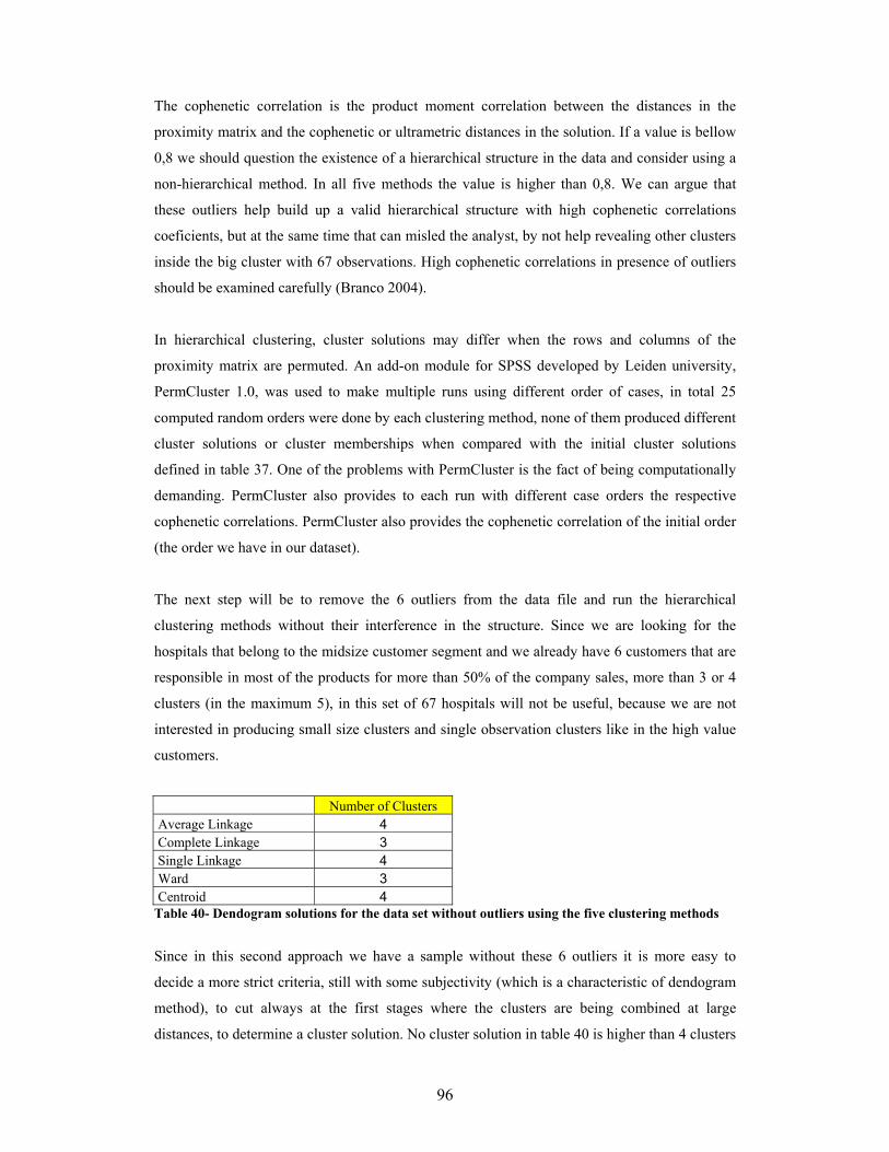
96
The cophenetic correlation is the product moment correlation between the distances in the
proximity matrix and the cophenetic or ultrametric distances in the solution. If a value is bellow
0,8 we should question the existence of a hierarchical structure in the data and consider using a
non-hierarchical method. In all five methods the value is higher than 0,8. We can argue that
these outliers help build up a valid hierarchical structure with high cophenetic correlations
coeficients, but at the same time that can misled the analyst, by not help revealing other clusters
inside the big cluster with 67 observations. High cophenetic correlations in presence of outliers
should be examined carefully (Branco 2004).
In hierarchical clustering, cluster solutions may differ when the rows and columns of the
proximity matrix are permuted. An add-on module for SPSS developed by Leiden university,
PermCluster 1.0, was used to make multiple runs using different order of cases, in total 25
computed random orders were done by each clustering method, none of them produced different
cluster solutions or cluster memberships when compared with the initial cluster solutions
defined in table 37. One of the problems with PermCluster is the fact of being computationally
demanding. PermCluster also provides to each run with different case orders the respective
cophenetic correlations. PermCluster also provides the cophenetic correlation of the initial order
(the order we have in our dataset).
The next step will be to remove the 6 outliers from the data file and run the hierarchical
clustering methods without their interference in the structure. Since we are looking for the
hospitals that belong to the midsize customer segment and we already have 6 customers that are
responsible in most of the products for more than 50% of the company sales, more than 3 or 4
clusters (in the maximum 5), in this set of 67 hospitals will not be useful, because we are not
interested in producing small size clusters and single observation clusters like in the high value
customers.
Number of Clusters Average Linkage 4 Complete Linkage 3 Single Linkage 4 Ward 3 Centroid 4
Table 40- Dendogram solutions for the data set without outliers using the five clustering methods
Since in this second approach we have a sample without these 6 outliers it is more easy to
decide a more strict criteria, still with some subjectivity (which is a characteristic of dendogram
method), to cut always at the first stages where the clusters are being combined at large
distances, to determine a cluster solution. No cluster solution in table 40 is higher than 4 clusters

97
what seems fit to our purpose. The dendograms outputs supporting the suggested number of
clusters are reported in appendix C.
Ward
0
5
10
15
20
25
30
35
40
10987654321
Number of Clusters
Agg
lom
erat
ion
Coe
ffici
ents
Centroid
0
0,5
1
1,5
2
2,5
3
3,5
4
10987654321
Number of Clusters
Agg
lom
erat
ion
Coe
ffici
ents
Single Linkage
0
0,1
0,2
0,3
0,4
0,5
0,6
0,7
0,8
0,9
151413121110987654321
Number of Clusters
Agg
lom
erat
ion
Coe
ffici
ents
Complete Linkage
0123456789
10
10987654321
Number of Clusters
Agg
lom
erat
ion
Coe
ffici
ents
Average Linkage
0
0,5
1
1,5
2
2,5
3
3,5
4
4,5
10987654321Number of Clusters
Agg
lom
erat
ion
Coe
ffici
ents
Figure 19- Agglomeration coefficient graphs for the 5 clustering methods without outliers
Probably a 2 or 3 cluster solutions occur in ward method but the elbow is not very clear, the
centroid and the average linkage methods suggest a 4 cluster solution, the complete linkage a 5
cluster solution and finally the single linkage method suggests a 2, 4 and 12 cluster solutions.
Mojena (last 12 cluster solutions)
Number of clusters in
the solution Ward Centroid Single
Linkage Complete Linkage
Average Linkage
12 0,07 0,25 1,17 0,04 0,26 11 0,13 0,33 1,25 0,08 0,33 10 0,23 0,39 1,35 0,17 0,39 9 0,36 0,62 1,41 0,38 0,45 8 0,59 0,82 1,45 0,41 0,72 7 0,82 0,88 1,48 0,70 0,95 6 1,05 1,02 1,49 0,85 1,14 5 1,54 1,04 1,58 1,54 1,42 4 2,28 2,36 3,00 2,37 2,61 3 3,48 4,40 3,05 3,75 4,22 2 6,13 5,38 4,10 6,01 5,33
Table 41- Values for the last cluster solutions without outliers using the Mojena criteria
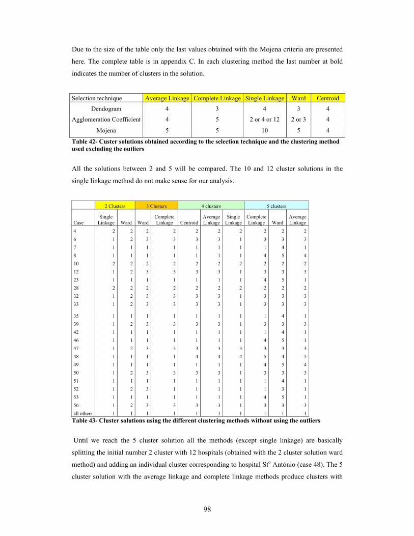
98
Due to the size of the table only the last values obtained with the Mojena criteria are presented
here. The complete table is in appendix C. In each clustering method the last number at bold
indicates the number of clusters in the solution.
Selection technique Average Linkage Complete Linkage Single Linkage Ward Centroid
Dendogram 4 3 4 3 4
Agglomeration Coefficient 4 5 2 or 4 or 12 2 or 3 4
Mojena 5 5 10 5 4
Table 42- Custer solutions obtained according to the selection technique and the clustering method used excluding the outliers
All the solutions between 2 and 5 will be compared. The 10 and 12 cluster solutions in the
single linkage method do not make sense for our analysis.
2 Clusters 3 Clusters 4 clusters 5 clusters
Case Single
Linkage Ward Ward Complete Linkage Centroid
Average Linkage
Single Linkage
Complete Linkage Ward
Average Linkage
4 2 2 2 2 2 2 2 2 2 2 6 1 2 3 3 3 3 1 3 3 3 7 1 1 1 1 1 1 1 1 4 1 8 1 1 1 1 1 1 1 4 5 4 10 2 2 2 2 2 2 2 2 2 2 12 1 2 3 3 3 3 1 3 3 3 23 1 1 1 1 1 1 1 4 5 1 28 2 2 2 2 2 2 2 2 2 2 32 1 2 3 3 3 3 1 3 3 3 33 1 2 3 3 3 3 1 3 3 3
35 1 1 1 1 1 1 1 1 4 1 39 1 2 3 3 3 3 1 3 3 3 42 1 1 1 1 1 1 1 1 4 1 46 1 1 1 1 1 1 1 4 5 1 47 1 2 3 3 3 3 3 3 3 3 48 1 1 1 1 4 4 4 5 4 5 49 1 1 1 1 1 1 1 4 5 4 50 1 2 3 3 3 3 1 3 3 3 51 1 1 1 1 1 1 1 1 4 1 52 1 2 3 1 1 1 1 1 3 1 53 1 1 1 1 1 1 1 4 5 1 56 1 2 3 3 3 3 1 3 3 3 all others 1 1 1 1 1 1 1 1 1 1
Table 43- Cluster solutions using the different clustering methods without using the outliers
Until we reach the 5 cluster solution all the methods (except single linkage) are basically
splitting the initial number 2 cluster with 12 hospitals (obtained with the 2 cluster solution ward
method) and adding an individual cluster corresponding to hospital Sto António (case 48). The 5
cluster solution with the average linkage and complete linkage methods produce clusters with

99
very small sizes and clusters of one element, more prominent in the average linkage, not being
very useful methods for our purpose. The 5 cluster solution with the ward method is able to
produce 4 clusters with 22 hospitals and a big cluster with 45 hospitals. Of all the methods in
table 43, the ward method in the 5 cluster solution is the one that is able to produce a more
meaningful solution to the business.
Another very important fact is that cluster number 2 of the two cluster solution in table 43
produces the same cluster membership of the number 2 cluster in the 5 cluster solution of the
ward method with all the hospitals, and reinforces the possible use of this solution. The table
bellows (table 44) summarizes the initial ward 5 cluster solution with all the hospitals.
By analysing table 44, the mean of each variable in the midsize value segment is higher than in
the low value segment, but the total sales of the different products is still higher than 20% in
several products in the low value segment. Specifically with product B and product D the means
Ward Method
Total Calls Patients
Product B
Product A
Product C
Product D
Product F
Product E
Total Guideline
Factor I
Factor II
Factor II
Mean 16,3 268,8 4,2 31,9 2,6 16,9 0,2 1,6 20,4 -0,4 -0,1 -0,2
Sum 895,0 14782,0 231,0 1755,0 144,0 927,0 10,0 87,0 1122,0
Low
Val
ue
1 N=55 (75,3%) % of
Total Sum 16,8 35,6 34,2 24,5 14,5 33,4 7,7 23,3 22,2
Mean 114,7 825,7 5,3 118,6 37,8 30,3 0,0 9,3 108,2 0,7 -0,5 0,2
Sum 1376,0 9908,0 64,0 1423,0 453,0 364,0 0,0 112,0 1298,0
Mid
size
Va
lue 2
N=12 (16,4%) % of Total Sum 25,9 23,9 9,5 19,9 45,5 13,1 0,0 30,0 25,7
Mean 495,3 3830,0 61,7 761,3 83,0 106,7 11,7 2,0 450,7 3,9 0,5 -1,1
Sum 1486,0 11490,0 185,0 2284,0 249,0 320,0 35,0 6,0 1352,0 3
(Conventional Drugs Users)
N=3 (4,1%) % of Total Sum 27,9 27,7 27,4 31,9 25,0 11,5 26,9 1,6 26,8
Mean 716,0 2273,0 150,0 800,0 23,0 808,0 35,0 0,0 436,0 0,2 7,0 -0,8
Sum 716,0 2273,0 150,0 800,0 23,0 808,0 35,0 0,0 436,0
4 (High Users
of Innovative Drugs)
N=1 (1,4%) % of Total Sum 13,5 5,5 22,2 11,2 2,3 29,1 26,9 0,0 8,6
Mean 422,0 1521,0 23,0 446,0 63,0 179,5 25,0 84,0 418,0 0,9 0,8 5,2
Sum 844,0 3042,0 46,0 892,0 126,0 359,0 50,0 168,0 836,0
Hig
h Va
lue
5 (High Product
E) N=2 (2,7%) % of
Total Sum 15,9 7,3 6,8 12,5 12,7 12,9 38,5 45,0 16,6
Mean 72,8 568,4 9,3 98,0 13,6 38,1 1,8 5,1 69,1 0,0 0,0 0,0Total (N=73) Sum 5317,0 41495,0 676,0 7154,0 995,0 2778,0 130,0 373,0 5044,0
Table 44- Dashboard for the 5 cluster solution with ward method including all observations

100
are close between these two segments and the maximum values of these two products are higher
in the low value segment (see appendix C, for more information about the descriptive statistics
of each cluster). The high value segment has three sub-segments: the Conventional Drugs users,
being the main characteristics of this cluster the high usage of Product A and C and the high
mean of chemotherapy patients, making this a high potential cluster for growth in the innovative
drugs; High users of innovative drugs (only one hospital), being the main characteristics of this
cluster the high usage of Product B, D and F; High Product E, where only two hospitals make
45,0% of the sales of product E. Another important characteristic of the high value segment is
that 92% of the sales of product F belong to this segment, because this is a very specific drug
that requires specific conditions that usually can only be found in central hospitals and oncology
specialized hospitals.
Ward Method
Total Calls Patients
Product B
Product A
Product C
Product D
Product F
Product E
Total Guideline
Factor I
Factor II
Factor III
1 Mean 7,0 175,4 0,0 19,7 1,5 3,0 0,0 0,1 10,0 -0,4 -0,2 -0,2
N= 45 (61,6%) Sum 314,0 7893,0 0,0 887,0 69,0 137,0 0,0 4,0 450,0
Low
Val
ue
% of Total Sum 5,9 19,0 0,0 12,4 6,9 4,9 0,0 1,1 8,9
2 Mean 151,3 937,0 14,7 145,7 36,0 26,0 0,0 32,7 130,0 0,6 -0,5 1,4
N= 3 (4,1%) Sum 454,0 2811,0 44,0 437,0 108,0 78,0 0,0 98,0 390,0
% of Total Sum 8,5 6,8 6,5 6,1 10,9 2,8 0,0 26,3 7,7
3 Mean 102,4 788,6 2,2 109,6 38,3 31,8 0,0 1,6 100,9 0,7 -0,5 -0,3
N=9 (12,3%) Sum 922,0 7097,0 20,0 986,0 345,0 286,0 0,0 14,0 908,0
% of Total Sum 17,3 17,1 3,0 13,8 34,7 10,3 0,0 3,8 18,0
4 Mean 82,2 898,6 21,8 119,4 11,4 126,0 2,0 0,0 93,6 0,0 0,6 -0,5
N=5 (6,8%) Sum 411,0 4493,0 109,0 597,0 57,0 630,0 10,0 0,0 468,0
% of Total Sum 7,7 10,8 16,1 8,3 5,7 22,7 7,7 0,0 9,3
5 Mean 34,0 479,2 24,4 54,2 3,6 32,0 0,0 16,6 40,8 -0,5 0,1 0,5
N=5 (6,8%) Sum 170,0 2396,0 122,0 271,0 18,0 160,0 0,0 83,0 204,0
Mid
size
Val
ue
% of Total Sum 3,2 5,8 18,0 3,8 1,8 5,8 0,0 22,3 4,0
Mean 72,8 568,4 9,3 98,0 13,6 38,1 1,8 5,1 69,1 0,0 0,0 0,0Total* Sum 5317 41495 676 7154 995 2778 130 373 5044
Table 45- Dashboard for the 5 cluster solution with ward method excluding the outliers *the total is calculated for the total observations including the outliers.

101
The previous analysis didn’t assure us if the midsize customer segment was really well
determined (seen in table 44). As mentioned before the 5 cluster solution using ward method in
the analysis excluding the outliers produced a possible meaningful solution that it is confirmed
by table 45. In this case the low value segment is really of low impact (less than 20%) in all
variables. In the midsize customer segment it is possible to split this segment in four sub-
segments each with their own distinctive characteristics: Cluster 2, high product E usage;
Cluster 3, high product C usage; Cluster 4 high product D and B usage. Cluster 5 high product E
and B usage. The numbers at bold in the table 45, point out for the main characteristic of the
cluster, particularly in terms of their mean and % of sum of total.
.
Cophenetic Correlation Average linkage Single linkage Complete linkage Ward Centroid
0,869 0,835 0,769 0,714 0,868 Table 46- Dashboard for the 5 cluster solution with ward method excluding the outliers
The cophenetic correlations obtained for the five clustering methods when we exclude the
outliers was lower than 0,8 in two of the methods, including the ward method that produce the
most interpretable solution for our purpose, and if the value is bellow 0,8 we should question
the use of the hierarchical method, to be more precise the cophenetic correlation is a measure of
how faithfully a dendrogram preserves the pairwise distances between the original unmodeled
data points.
Again PermCluster 1.0, was used to make multiple runs using different order of cases, in total
25 computed random orders were done by each clustering method, none of them produced
different cluster solutions or memberships when compared with the initial cluster solutions
defined in table 43.
If the objective of the hierarchical clustering was only to find the most valuable customers, the
five different clustering methods are aligned, but when we want to have a solution that finds a
middle segment with all the hospitals included in the analysis we only get one solution with the
ward method, that is not able to clearly separate the midsize customers from the low value
customers in terms of the clusters produced. If we exclude the outliers it is the ward method that
produces the most interpretable solution that clearly identifies the low value customers and
separates them from the clusters that represent the midsize customers segment, nevertheless
having this method a cophenetic correlation bellow 0,8, we should question the existence of a
hierarchical structure in the data. Considering the complexity around using all these different
hierarchical agglomerative clustering methods to find the ideal and most interpretable solution,

102
the difficulty of dealing with outliers and the different solution obtained by these methods that
are not always convergent, a non-hierarchical method, preferably robust to outliers should be
used.
To overcome the difficulties found in hierarchical clustering analysis we need an algorithm
robust to outliers. The idea is to find algorithms which degrade progressively in the presence of
outliers instead of abruptly disrupting the clustering structure. Several studies revealed the
quality of Self- Organizing Maps (SOMs) to deal with datasets with this problem and their
superiority over k-means algorithm (Bação et al. 2004; Openshaw and Openshaw 1997;
Openshaw et al. 1995) and for this reason was the selected non-hierarchical method to be used
in this study.
SOMs have been tested in several areas, but there use in marketing is not as common as other
methods like k-means. In the pharmaceutical market there are several reasons to use SOMs,
specifically their ability to deal with large datasets, their superiority over k-means specially in
data with outliers and the fact that the customers in the pharmaceutical industry, like the
hospitals, are geo-referenced data, what makes possible and very useful the use of Geo-SOMs
(Bação et al. 2005), although GEO-SOMs are out of the scope of this thesis.
The several functionalities allowed by SOM toolbox for Matlab enable for example the use of
SOMs as data exploratory tool. There is a very easy way to make a first analysis of our data by
using the function som_make. It is a convenient function that combines the tasks of creating,
initializing and training a SOM, using pre-default criteria’s (Vesanto et al. 2000). In our first
approach the initial data was checked for possible correlations between the variables, using the
component planes as an alternative method to the correlation matrix. The som_make function
was used and the results are present bellow.

103
Figure 20- Component planes for the original variables If no analysis as been conducted previously it was possible to check the presence of strong
correlations between variables, a very clear example is visualized between Total calls, Product
A and Total Guideline, suggesting for the possible use of Factor analysis with the purpose
already described in this study.
Our objective is to define clusters using the computed factor scores obtained by factor analysis.
The U-matrix constitutes a particularly useful tool to analyse the results of a SOM, as it allows
an appropriate interpretation of the clusters available in the data. The U-matrix is a
representation of a SOM in which distances, in the input space, between neighbouring neurons
are represented, usually using a colour or grey scale. If distances between neighbouring neurons
are small, then these neurons represent a cluster of patterns with similar characteristics. If the
neurons are far apart, then they are located in a zone of the input space that has few patterns,
and can been seen as a separation between clusters.
A SOM and their corresponding U-matrix and component planes must be obtained using the
previously computed factor scores. The training parameters were as follows: “Initialization:
random”; “map shape: sheet”; “lattice: rectangular”; “number of units: 9x8”; neighbourhood
function: Gaussian”; “training type: sequential train”; “number of training phases: 2”; “learning
rate function: linear”; parameters of 1st phase: radius_ini=8, alpha_ini=0.5, epochs=100”;
parameters of 2nd phase: radius_ini=4, alpha_ini=0.2, epochs=200”. In both training phases the
radius decrease to 1. The analysis was repeated with the double of epochs (in appendix D the
matlab code used is described).

104
In total 30 runs were done using the defined training parameters and the obtained maps were all
similar. The analysis with the double of epochs reached the same results compared to the initial
epochs.
Figure 21- U-matrix with neurons labelled
Figure 22- U-matrix with the hits and clusters pointed out. Small distances are represented at blue while large are at red
The typical U-matrix obtained in our analysis is presented in figure 22. Besides what as already
been mentioned about how to identify clusters in the U-matrix, the fact that some units are not
best matching unit (BMU) of any input pattern, helped in the identification of our clusters (by
helping defining the borders), also important to note is that the size of the superimposed black
squares are proportional to the number of hits.
The analysis of the U-matrix leads to the same clustering of our high value customers that as
already presented before in the hierarchical analysis. A middle segment seems to be represented
by cluster 3, whereas cluster 2 seems to be more similar to cluster 1 but it is separated by a
border of units that are not BMU of any input pattern. In theory we could regard clusters 1, 2

105
and 3 as sub-groups of one big cluster, but taking in account the presence of 6 outliers and the
impact they produce in the distances in the U-matrix, these 3 sub-groups (more evident the sub-
group characteristics between cluster 1 and 2), could be considered as independent market
segments. Another important fact that should be of our attention is that neuron 65 in cluster 1,
shows a huge superimposed black square that is proportional to a very large number of hits.
More important is to check the business interpretability of our solution.
te qe 0,082 0,353
Table 47- Average quantization (qe) and topological errors (te) obtained. The topology error in the final phase, as calculated by the Somtoolbox, was around 8%, which
indicates a fairly good unfolding (Lobo et al 2004), considering we are mapping a dataset with
outliers.
Figure 23- SOM component planes
By using the component planes we can notice that what differentiates cluster 4 is Factor II
(Innovative), while cluster 5 is differentiated by Factor III (Alternative) with high product E
usage and finally cluster 6 is differentiated by Factor I (Conventional). The cluster membership
of these specific clusters correspond to exactly the same that was previously mentioned to the
high value customers, demonstrating how easily the component planes identify and
differentiates the main characteristics of the company most important customers. From the
marketing point of view and with the purpose of strategic tactical implementation, component
planes can be very useful, because marketing people can visualize, for example, where is the
cluster with the highest impact in the innovative drugs, being in this case cluster 4 and its only
member, hosp. Sta Maria, knowing this they can implement strategies to maintain this

106
performance in this specific cluster or for example they know when they launch a new
innovative drug what is the cluster with the highest probability of usage adoption of the new
drug. Cluster 3 seems to be influenced by factor III. Cluster 1 and 2 doesn’t seem to be
differentiated specifically by any of the 3 components.
SOM Method Total Calls Patients
Product B
Product A
Product C
Product D
Product F
Product E
Total Guideline
Factor I
Factor II
Factor III
1 Mean 9,1 176,8 0,0 22,8 1,8 3,0 0,0 0,1 11,3 -0,4 -0,2 -0,2
N= 46 (63,0%) Sum 418,0 8132,0 0,0 1047,0 81,0 137,0 0,0 4,0 518,0
Low
Val
ue
% of Total Sum 7,9 19,6 0,0 14,6 8,1 4,9 0,0 1,1 10,3
2 Mean 66,5 867,6 11,3 106,6 26,9 64,2 0,9 0,0 85,8 0,4 -0,1 -0,4
N= 11 (15,1%) Sum 731 9543 124 1172 296 706 10 0 944
% of Total Sum 13,8 23,0 18,3 16,4 29,8 25,4 7,7 0,00 18,7
3 Mean 112,2 701,5 17,1 95,9 22 44,8 0 19,5 95,8 0,2 -0,2 0,7
N=10 (13,7%) Sum 1122,0 7015,0 171,0 959,0 220,0 448,0 0,0 195,0 958,0 M
idsi
ze V
alue
High E % of Total Sum 21,1 16,9 25,3 13,4 22,1 16,1 0,0 52,3 19,0
4 Mean 716 2273 150 800 23 808 35 0 436 0,2 7,0 -0,8 N=1
(1,4%) Sum 716 2273 150 800 23 808 35 0 436 (High Users of Innovative
Drugs)
% of Total Sum 13,5 5,5 22,2 11,2 2,3 29,1 26,9 0,0 8,6
5 Mean 422,0 1521,0 23,0 446,0 63,0 179,5 25,0 84,0 418,0 0,9 0,8 5,2 N=2
(2,7%) Sum 844,0 3042,0 46,0 892,0 126,0 359,0 50,0 168,0 836,0
(High Product E)
% of Total Sum 15,9 7,3 6,8 12,5 12,7 12,9 38,5 45,0 16,6
6 Mean 495,3 3830,0 61,7 761,3 83,0 106,7 11,7 2,0 450,7 3,9 0,5 -1,1 N=3
(4,1%) Sum 1486,0 11490,0 185,0 2284,0 249,0 320,0 35,0 6,0 1352,0
Hig
h Va
lue
(Conventional Drugs Users)
% of Total Sum 27,9 27,7 27,4 31,9 25,0 11,5 26,9 1,6 26,8
Mean 72,8 568,4 9,3 98 13,6 38,1 1,8 5,1 69,1 0 0 0
Total Sum 5317 41495 676 7154 995 2778 130 373 5044 Table 48- Dashboard with the SOM clustering solution
The dashboard above summarizes the results obtained with SOM clustering. The high value
customers were identified the same way like in the hierarchical clustering but a much more
meaningful midsize customer segment is identified with cluster 2 and cluster 3, without the need
to exclude the high value customers from the analysis like in the hierarchical clustering. Also
the balanced size of both clusters 2 and 3 in number of hospitals is much more adequate to a
practical approach to this segment than the solutions obtained with hierarchical clustering.
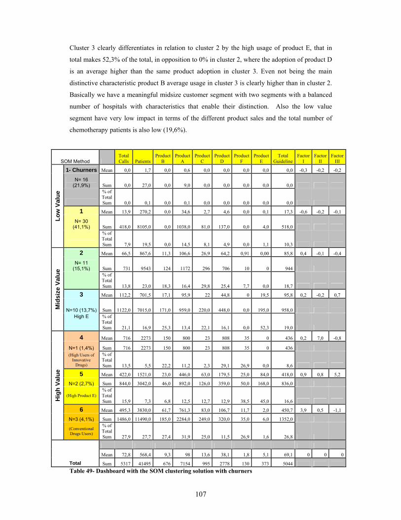
107
Cluster 3 clearly differentiates in relation to cluster 2 by the high usage of product E, that in
total makes 52,3% of the total, in opposition to 0% in cluster 2, where the adoption of product D
is an average higher than the same product adoption in cluster 3. Even not being the main
distinctive characteristic product B average usage in cluster 3 is clearly higher than in cluster 2.
Basically we have a meaningful midsize customer segment with two segments with a balanced
number of hospitals with characteristics that enable their distinction. Also the low value
segment have very low impact in terms of the different product sales and the total number of
chemotherapy patients is also low (19,6%).
SOM Method Total Calls Patients
Product B
Product A
Product C
Product D
Product F
Product E
Total Guideline
Factor I
Factor II
Factor III
1- Churners Mean 0,0 1,7 0,0 0,6 0,0 0,0 0,0 0,0 0,0 -0,3 -0,2 -0,2
N= 16 (21,9%) Sum 0,0 27,0 0,0 9,0 0,0 0,0 0,0 0,0 0,0
% of Total Sum 0,0 0,1 0,0 0,1 0,0 0,0 0,0 0,0 0,0
1 Mean 13,9 270,2 0,0 34,6 2,7 4,6 0,0 0,1 17,3 -0,6 -0,2 -0,1
N= 30 (41,1%) Sum 418,0 8105,0 0,0 1038,0 81,0 137,0 0,0 4,0 518,0
Low
Val
ue
% of Total Sum 7,9 19,5 0,0 14,5 8,1 4,9 0,0 1,1 10,3
2 Mean 66,5 867,6 11,3 106,6 26,9 64,2 0,91 0,00 85,8 0,4 -0,1 -0,4
N= 11 (15,1%) Sum 731 9543 124 1172 296 706 10 0 944
% of Total Sum 13,8 23,0 18,3 16,4 29,8 25,4 7,7 0,0 18,7
3 Mean 112,2 701,5 17,1 95,9 22 44,8 0 19,5 95,8 0,2 -0,2 0,7
N=10 (13,7%) Sum 1122,0 7015,0 171,0 959,0 220,0 448,0 0,0 195,0 958,0 Mid
size
Val
ue
High E % of Total Sum 21,1 16,9 25,3 13,4 22,1 16,1 0,0 52,3 19,0
4 Mean 716 2273 150 800 23 808 35 0 436 0,2 7,0 -0,8
N=1 (1,4%) Sum 716 2273 150 800 23 808 35 0 436 (High Users of
Innovative Drugs)
% of Total Sum 13,5 5,5 22,2 11,2 2,3 29,1 26,9 0,0 8,6
5 Mean 422,0 1521,0 23,0 446,0 63,0 179,5 25,0 84,0 418,0 0,9 0,8 5,2
N=2 (2,7%) Sum 844,0 3042,0 46,0 892,0 126,0 359,0 50,0 168,0 836,0
(High Product E) % of Total Sum 15,9 7,3 6,8 12,5 12,7 12,9 38,5 45,0 16,6
6 Mean 495,3 3830,0 61,7 761,3 83,0 106,7 11,7 2,0 450,7 3,9 0,5 -1,1
N=3 (4,1%) Sum 1486,0 11490,0 185,0 2284,0 249,0 320,0 35,0 6,0 1352,0
Hig
h Va
lue
(Conventional Drugs Users)
% of Total Sum 27,9 27,7 27,4 31,9 25,0 11,5 26,9 1,6 26,8
Mean 72,8 568,4 9,3 98 13,6 38,1 1,8 5,1 69,1 0 0 0
Total Sum 5317 41495 676 7154 995 2778 130 373 5044 Table 49- Dashboard with the SOM clustering solution with churners

108
An analysis to big superimposed black square corresponding to unit 65, revealed 16 hospital
with almost null value to the company both in terms of product sales and also in terms of
chemotherapy patients (0,1%), assuring us that no oncology potential exists even if sales are not
made to them. These are small hospitals that very rarely buy oncology products or only have
done it once, because of a specific situation, and are what we can call in CRM, “churners” and
correspond to about 22% of the hospitals in the company database. So it can make sense to
subdivide cluster 1 between the low value customers and the ones with no value at all. That
shows how useful can be the U-matrix to do such analysis. Clearly the best dashboard to be sent
to the management of this specific pharmaceutical company should be the one with the artificial
division of cluster 1 (table 49), were an efficient prune of the “no value hospitals” is done by a
specific unit in the U-matrix. Overall the results of our clusters demonstrate that the clusters
pointed out in the U-matrix provided meaningful solutions.
The analysis of the U-matrix is always touched with some subjectivity whereas hierarchical
methods are guided with more tight rules to define the number of clusters, but if the analyst is
aware of the type of data that is dealing with and takes the advantage of the flexibility of the
SOM method to deal with it, for example, with outliers, for sure it as very useful method. SOM
is a robust method to outliers that enables the identification of sub-groups that have small
differences but at the same time meaningful, that in the hierarchical methods can be affected by
outliers and not be revealed. Overall our analysis confirmed these assumptions and SOM
produced a more meaningful business solution in a much more easy fashion and generally
outperformed the hierarchical methods even with a dataset with a relatively small number of
cases (N=73). Nevertheless if we are willing to make a first analysis with the outliers and
secondly exclude them and use specifically the ward method we could also find an interpretable
business solution with this hierarchical method. SOM method demonstrated that can be a very
useful tool to be used even in smaller datasets, especially in cases where outliers are present.
Method Comments
Hierarchical
Clustering
The five different agglomeration methods basically spited our dataset in one big cluster and small clusters representing the outlier hospitals that represent in value the most important hospitals. From the business point of view it should be important to have a midsize customer segment by splitting the hospitals in the big cluster in two or more clusters. A second analysis was conducted without the atypical hospitals, but the five different methods were not convergent in the solutions provided. In terms of business interpretability ward method provided the best solution but the cophenetic correlation bellow 0,8 indicates that a non-hierarchical method should be used.
SOM The SOM algorithm showed the capacity to degrade progressively in the presence of outliers instead of abruptly disrupting the clustering structure. So it was possible by using the U-matrix to segment all the hospitals in the dataset, without the need to exclude the outliers. Even if the analysis of the U-matrix is touched with some subjectivity the clusters identified enabled the identification of 3 clusters of high value customers, 2 clusters in the midsize customer segment and one cluster of low value customers with one specific unit that identifies the churners or the customers of very low value (that have not been identified by the hierarchical methods). The SOM method provided a meaningful business solution without the need to exclude the outliers in opposition to the hierarchical methods that required these to be excluded, increasing the complexity of the analysis and also the different methods did not converge to the same solution when the outliers were excluded.
Table 50- Differences between the hierarchical methods and SOM in terms of the results achieved

109
The use of SOMs in CRM, even in earlier stages where the number of variables and the number
of cases in the dataset are small, like in our case, demonstrated to be useful, moreover with the
growth of the data in the CRM system is a method that is able to deal with large datasets
whereas hierarchical methods are not and also have a propensity to outperform other non-
hierarchical methods like k-means (Lobo et al. 2004).

110
5. CONCLUSIONS AND FUTURE DEVELOPMENTS ______________________________________________________________________ Due to the very limited information published about CRM in the pharmaceutical industry the
literature revision in this thesis plays a very important role. The so-far-described CRM approach
does not yet seem completely adapted to the complexity of the health care industry. Also in the
pharmaceutical marketing the product focus approach it is still dominant versus the customer
centric approach, what is a clear obstacle to the success of a CRM program. Nevertheless the
United States seems to be more advanced than Europe in all the different approaches of CRM,
probably because the legislation in the United States it is more liberal, allowing DTC
advertising and in the United States there is also the possibility to get prescribing information
per physician. Overall the CRM in the pharmaceutical industry is far-behind, when compared
with other business areas, like consumer goods, finance (banking) or insurance companies. One
of the big obstacles for the success of CRM in the pharmaceutical industry is the poor analytics
applied to the current CRM programs, being this problem more acute in Europe than in United
States. Specifically in terms of program implementation three different strategies have been
applied in the pharmaceutical industry, based on: sales force automation systems; online
strategies and communication technologies; supply chain and demand management integration.
Overall the biggest difference between the CRM programs in Europe and United States is the
fact that the focus in the patient in the United States is bigger and deeper than in Europe in
terms of CRM programs. In the last European Sales Force Effectiveness Summit for
Pharmaceutical industry held in 2006 (Eyeforfarma 2006), CRM was the main topic, but almost
all the European CRM approaches presented where focused in the physician or health care
providers and in improving CRM SFA tools. The analytics presented to support the European
CRM system were extremely poor, segmentation methodologies were very rudimentary, for
example physician segmentation presented was based on empirical rules without any statistical
validation. We can resume that CRM programs in Europe were developed around physicians or
health care providers as the main target, with some examples of internet use to target patients, in
contrast with more sophisticated CRM programs in United States targeting patients and
physicians, considering them equally important.
It was one of our objectives to find relationships between the business variables in the company
CRM dataset in order to give evidence to the marketing department which variables correlate
together and can help driving the sales of the different products, and also to deploy multi-
product sales force that will promote products that share common business characteristics, by

111
using factor analysis it was possible to conduct this assessment. In our analysis all the different
business variables load highly only in one factor.
Overall 3 factors were extracted and labelled as: Factor I – Conventional (where conventional
products, sales representative activities and chemotherapy patients load high); Factor II-
Innovative (where innovative products load high); Factor III- Alternative (where product E that
is an alternative therapy to product D load high).
It seems that there is a clearly distinction between the innovative drugs and the conventional
drugs and it is reflected by the way they load highly in different factors. It makes sense to have a
sales force trained to promote Product A and C because we know that there treatment adoption
is strongly correlated between them (they load high in Factor I). It should also make sense to
have a sales force, focusing in the innovative products (B, D and F) because they are strongly
correlated between themselves (they load high in Factor II).
By assessing which products load highly in each factor we can suggest deployment of multi-
product sales forces, being particularly more important and reliable if these products like in our
case (oncology) belong all to a specific therapeutic area, because the target customers
(physicians) will be the same. By doing these, pharmaceutical companies can improve their
sales and marketing effectiveness, avoid building up sales forces promoting only one product
and save money by having less sales representatives in the field and can develop marketing
strategies that promote synergies between products.
Also important for the sales and marketing teams is to be aware that the consumption of the
company conventional pharmaceutical drugs (product A and C) is related with the number of
chemotherapy patients treated in each hospitals and any change in the number of chemotherapy
patients treated could have an impact in the company sales of these products.
Also important is that the sales force promotional effort (number of visits made by the sales
representatives) is more strongly correlated with the consumption of the conventional products
than the innovative products, so a specific guideline for visiting should be implemented if a
multi-product sales force promoting innovative products is deployed.
The third Factor gives a clear message to the marketing department to be aware that the more
recently launched product E has a different treatment adoption pattern across hospitals,
compared with product D. Product E only loads highly in third factor and it is an equal
pharmaceutical drug to product D in terms of therapeutic indication. Here value equity plays an

112
important role and the company could benefit if the hospitals switch from D to E, so this
product can be promoted by a sales force of innovative drugs that can promote product D switch
to E, avoiding in this specific situation a mono-product sales force.
Provide customer segmentation that can be meaningful to the pharmaceutical company business
by enabling the alignment between sales and marketing strategies using the company CRM
dataset was also another objective. Currently a good customer segmentation should identify not
only the high value customers but segment them by their characteristics (Pepers and Rogers
2006), identify the midsize customers, because usually they demand good service in a
reasonable way, pay nearly full price, and are often the most profitable (Kotler and Keller 2007)
and identify the low value customers, specifically the ones that the company should not invest
promotional effort. A specific segmentation was obtained by using SOMs that is aligned with
the business assumptions previously mentioned and make sense in the current hospital market
that with the current governmental price pressures and tender negotiations in hospitals is
changing to a type of market similar to other industries like the consumer goods. In the U-
matrix was possible to identify 6 clusters, 3 clusters belonging to high value customers grouped
by their different characteristics (high users of conventional products; high users of innovative
drugs; high users of product E), 2 clusters identify the midsize customer segment (being one of
the clusters of high users of product E) and one cluster that identifies the low value customers
where one unit in the U-Matrix in this cluster identifies the very low value hospitals, that
besides the fact they rarely buy products to the company, the patients treated with chemotherapy
in these hospitals is almost zero, being hospitals where the oncology potential is almost null and
no promotional effort should be spent (table 49 provides the quantitative characteristics of the
SOM segmentation), taking in consideration the current high cost of sales force visiting in the
pharmaceutical industry, the identification of these customers is very importantant. An
important advantage of SOMs is that from the marketing point of view and with the purpose of
strategic tactical implementation, component planes can be very useful, because marketing
people can visualize graphically which hospitals have the highest impact from the three
different factors.
The Hierarchical methods were not so effective in finding a meaningful business solution like
SOMs. The five different agglomeration methods basically spited our dataset in one big cluster
and small clusters representing the outlier hospitals that represent in value the most important
hospitals. From the business point of view it should be important to have a midsize customer
segment by splitting the hospitals in the big cluster in two or more clusters. A second analysis
was conducted without the atypical hospitals, but the five different methods were not
convergent in the solutions provided. In terms of business interpretability ward method provided

113
the best solution (see table 45) between the hierarchical methods, with a clear segmentation of
customers in the midsize customer segment and the identification of a low value segment, but
with the disadvantage that we need to exclude first the high value hospitals because of their
outlier behaviour (common fact to all hierarchical methods) and in opposition to SOMs the very
low value customers are not easily identifiable (common fact to all hierarchical methods), also
the cophenetic correlation bellow 0,8 indicates that a non-hierarchical method should be used
and SOM was selected because of the method ability to degrade progressively in the presence of
outliers instead of abruptly disrupting the clustering structure (Bação et al. 2004; Openshaw and
Openshaw 1997; Openshaw et al. 1995). The comments produced about the differences
between the hierarchical methods and SOMs, meant to be contextualized with our thesis data
and business purpose and do not pretend to be regarded as a generalized comparison between
methods.
It was been shown that using the right multivariate techniques in a CRM-SFA tool belonging to
a pharmaceutical company is possible to improve sales and marketing effectiveness processes.
When we segment the pharmaceutical company customers (hospitals) using the factors scores
we are aligning the sales forces deployment based on the produced factors with the customer
segmentation characteristics, enabling synergies between strategic marketing decisions and the
tactical implementation of them in the field. For example a sales force that promotes innovative
drugs will face different challenges when approaching a cluster of customers like the high users
of conventional products, compared with the cluster of high users of innovative drugs. Being
both of them high value customers, different marketing strategies should be customized taking
in account the customers differences and a correct tactical implementation of them should be
applied to the sales force.

114
It can be useful to use the strategy applied in this thesis as a basis to enhance the current CRM
programs in the pharmaceutical industry based on SFA tools. The figure bellow shows the
concept to be applied:
Figure 24- ACE Concept for enhancement of the current CRM-SFA programs
The fact that the current CRM approach does not yet seem completely adapted to the
complexity of the pharmaceutical industry business as many players are involved in the health
care process, and each are having an increasingly defined role, clearly demonstrates that our
dataset is not exploiting all the variables that can be collected and analysed, inclusively not even
CLTV was calculated in the database. So ideally in future studies, if possible, a more complete
database with more variables, more cases and comparing different time frames should be used
and with larger datasets, datamining techniques should also be used.
Also an interesting approach that could be followed in future studies is conceptually defining
how to build a better CRM system in the pharmaceutical industry.
But using the literature revision done in this study other approaches to the pharmaceutical
industry could take place besides focus specifically in CRM, like studying more deeply the
business dynamics and the relationships established by the different relevant variables by using
confirmatory factor analysis. Also an approach with a CRM system based in a geographic
information system makes sense because the clients in the pharmaceutical industry, like
physicians or hospitals are easily geo-referenced.
ACE Strategy
Analysis of Businessattributes
Find relationships between them
Deploy multi-product sales forces
Develop marketing strategies that are aligned with
the relationships found between the business attributes
Develop a Customer segmentation that allows alignment with the
sales force deployment
Focus on:
Alignment: Between sales and marketing strategies.Customer: Provide meagniful segmentations
based on customer charactheistics.Efficiency: Reduce the number os sales forces
promoting products by deployingmulti-product sales forces

115
6. REFERENCES ______________________________________________________________________ Anderson, T. W. and H. Rubin (1956). "Statistical inference in factor analysis." Proceedings of
the Third Berkley Symposium on Mathematical Statistics and Probability 5: 111-150. Bação, F. (2005). Computational Inteligence in Geographic Information Science Problems: the
case of Zone Design, Universidade Nova de Lisboa- ISEGI. PhD. Bação, F., V. Lobo, et al. (2004). Clustering census data: comparing the performance of self-
organizing maps and k-means algorithms. KDNet Symposium: Knowledge-Based Services for the Public Sector. 3-4 June, Bonn, Germany.
Bação, F., V. Lobo, et al. (2005). "The self-organizing map, the Geo-SOM, and relevant
variations for geosciences." Computers & Geosciences 31: 155-163. Bard, M. (2007). "Tunnel Vision." Pharmaceutical Marketing Europe 4(1): 24-26. Bartlett, M. S. (1937). "The statistical concept of mental factors." British Journal of Psycology
28: 97-104. Branco, J. A. (2004). Uma Introdução à Análise de Clusters, Sociedade Portuguesa de
Estatística. Cangelosi, R. and A. Goriely (2007). "Component retention in principal component analysis
with application to cDNA microarray data." Biology Direct 2(2): 1-20. Carpenter, G. (2006). "In Close Contact." Pharmaceutical Marketing Europe 3(2): 24-26. CGEY and INSEAD (2002). Cracking the Code- Unlocking new value in customer
relationships. Datamonitor (2006). Optimizing Sales Force Effectiveness. Dolgin, K. (2007). Managing sales force change with simulation, IMS and Pharmaceutical
Marketing Europe. Eyeforpharma (2006). Sales force effectivenes for pharma companies. Sales force effectiveness
Europe 2006, Barcelona 13-15 March 2006. Garrat, J. (2006). "Outside the Box." Pharmaceutical Marketing Europe 3(4): 18-19. Gomes, P. J. (1993). Análise de Dados, Instituto Superior de Estatística e Gestão de Informação
Universidade Nova de Lisboa. Gower, J. C. (1971). "A generall coefficient of similarity and some of its properties." Biometrics
27: 857-872. IMS. (2007). "Global Pharmaceutical Sales by Region, 2006 " Retrieved 25 April, 2007, from
http://www.imshealth.com/ims/portal/front/articleC/0,2777,6025_80528184_80528215,00.html.
Johnson, R. A. and D. W. Wichern (1998). Applied Multivariate Statistical Analysis. New
Jersey, Prentice Hall.

116
Jolliffe, I. (2002). Principal Component Analysis. New York, Springer. Kiang, M. Y., M. Y. Hu, et al. (2006). "An extended self-organizing map network for market
segmentation: a telecommunication example." Decision Support Systems 42(1): 36-47. Kiang, M. Y., A. Kumar, et al. (2002). "Workshop on Artificial Intelligence: The application of
an Extended Self-Organizing Map Networks to Market Segmentation." Retrieved 20 October, 2007, from http://hdl.handle.net/2377/2246.
Kohonen, T., Ed. (2001). Self-Organizing Maps. Berlin-Heidelberger, Springer. Kotler, P. and K. l. Keller (2007). A framework for marketing management. New Jersey,
Prentice Hall. Lerer, L. (2002). "E- Business in the pharmaceutical industry." International Journal of Medical
Marketing 3(1): 69-73. Lerer, L. and M. Piper (2003). Digital Strategies in the Pharmaceutical Industry, Palgrave
Macmillan. Lien, C. H., A. Ramirez, et al. (2006). "Capturing and Evaluating Segments: Using Self-
Organizing Maps and K-Means in Market Segmentation." Asian Journal of Management and Humanity Sciences 1(1): 1-15.
Lobo, V., F. Bação, et al. (2004). The Self-Organizing Map and it’s variants as tools for
geodemographical data analysis: the case of Lisbon’s Metropolitan Area. AGILE 2004, 7th AGILE conference on Geographic Information Science. April 29th - May 1st, Heraklion, Greece.
Loureiro, M. (2006). Possiblistic Fuzzy Membership Using Self Organizing Maps- Application
To The Unsupervised Classification Of The Geodemographi Data Of The Metropolitan Area of Lisbon, Universidade Nova de Lisboa- ISEGI. Master Degree.
Malhotra, N. K. (2004). Marketing Research an applied orientation. New Jersey, Pearson
Prentice Hall. Milligan, G. W. and M. C. Cooper (1985). "An examination of procedures for determining the
number of clusters in a data set." Psychometrica 50: 159-179. Morgan, C. (2005). Not by Lists Alone, ZS Associates. Novartis. (2007). "bssucesszone." Retrieved 27 May, 2007, from
http://www.bpsuccesszone.com/. Openshaw, S., S. M. Blake, et al. (1995). "Using neurocomputing methods to classify Britain's
residential areas." Inovations in GIS 2: 97-111. Openshaw, S. and C. Openshaw (1997). Artificial inteligence in geography. Chichester, John
Wiley & Sons. Oracle and Peppers&RogeresGroup (2007). No More Limits: On Demand CRM Goes Strategic.
Oracle.

117
Peppers, D., M. Rogers, et al. (2007). "New Thinking on Lifetime Value." Return on Customer
Monthly (April 27 2006) Retrieved 5 June, 2007, from http://www.1to1media.com/View.aspx?DocID=29509.
PhRMA (2006).Pharmaceutical Industry Profile. Pharmaceutical Research and
Manufacturers of America. Rand, W. M. (1971). "Objective criteria for the evaluation of clustering methods." Journal of the
American Statistical Association 66: 846-850. Redwood, H. (2007). "Our Changing Vista." Pharmaceutical Marketing Europe 4(1): 18-19. Rencher, A. (1998). Multivariate Statistical Inference and Applications. New York, John Wiley
&Sons. Rushmeir, H., R. Lawrence, et al. (1997). Visualizing Customer Segmentations Produced by
Self Organizing Maps. Eighth IEEE Visualization 1997: 463. Schulman, K. A., L. E. Rubenstein, et al. (1996). "The Effect of Pharmaceutical Benefits
Managers: Is It Being Evaluated? ." Annals of Internal Medicine 124(10): 906-913. Sharma, S. (1996). Applied Multivariate Techniques, John Wiley & Sons. Thompson, B. (1993). "Calculation of standardized, noncentered factor scores: an alternative to
conventional factor scores." Perceptual and Motor Skills 77: 1128-1130. Thompson, E. (2005). Gartner's Top 54 CRM Case Studies, Sorted by Industry, for 2005,
Gartner. Turner, N. (1998). "The effect of common variance and structure pattern on random data
eigenvalues: Implications for the accuracy of parallel analysis." Educational and Psychological Measurement 58: 541-568.
Vesanto, J., J. Himberg, et al. (2000). SOM Toolbox for Matlab 5, Espoo, Helsinki University
of Technology: 59. Vilares, M. J. and P. S. Coelho (2005). A Satisfação e Lealdade do Cliente Metodologias de
Gestão, avaliação e Análise, Escolar Editora. Weinstein, L. and K. Rambo (2003). "Tomorrow's CRM: Big Picture and the Bottom Line."
Pharmaceutical Executive(May 2003): 84-90.

118
APPENDIX A ______________________________________________________________________ The descriptive statistics, the histogram, the boxplot, and the Kolmogorov-Smirnov statistic are
displayed for all our variables in the data. The Kolmogorov-Smirnov statistic tests the
hypothesis that the data are normally distributed. A low significance value (generally less than
0.05) indicates that the distribution of the data differs significantly from a normal distribution. If
there are less than 50 cases, the Shapiro-Wilk test is also displayed, even with more than 50
cases, 73 in total in our dataset the SPSS also displayed this test. Nevertheless the analysis of
the Kolmogorov-Smirnov statistic to all our variables demonstrated that all significantly differ
from a normal distribution.
Descriptives
72,84 17,34438,26
107,41
47,8010,00
21958,917148,185
0716716
61,502,794 ,2817,716 ,555
MeanLower BoundUpper Bound
95% ConfidenceInterval for Mean
5% Trimmed MeanMedianVarianceStd. DeviationMinimumMaximumRangeInterquartile RangeSkewnessKurtosis
Total CallsStatistic Std. Error
Table A.1- Descriptive statistics of total calls.
Tests of Normality
,312 73 ,000 ,553 73 ,000Total CallsStatistic df Sig. Statistic df Sig.
Kolmogorov-Smirnova Shapiro-Wilk
Lilliefors Significance Correctiona.
Table A.2- Normality test of total calls.
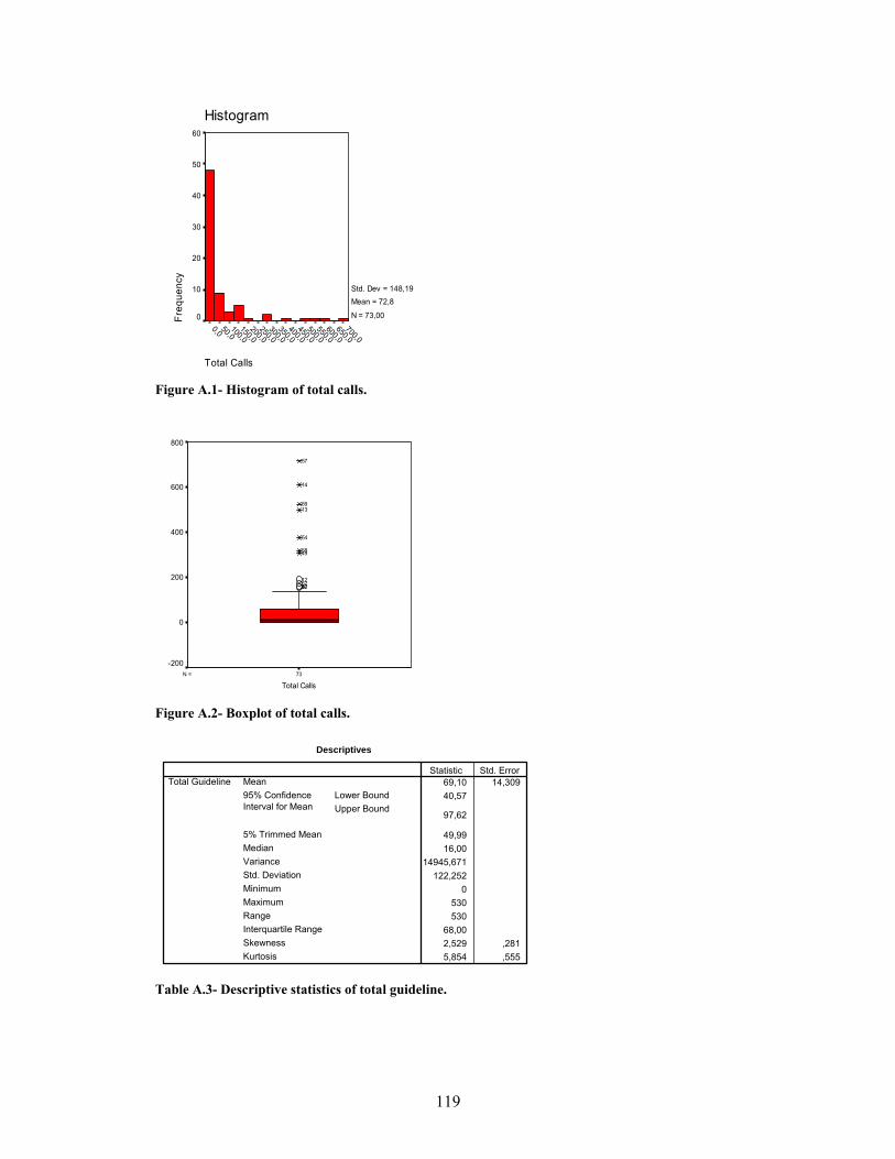
119
Total Calls
700,0650,0
600,0550,0
500,0450,0
400,0350,0
300,0250,0
200,0150,0
100,050,0
0,0
Histogram
Freq
uenc
y
60
50
40
30
20
10
0
Std. Dev = 148,19 Mean = 72,8
N = 73,00
Figure A.1- Histogram of total calls.
73N =
Total Calls
800
600
400
200
0
-200
304375212
4958
54
1359
14
57
Figure A.2- Boxplot of total calls.
Descriptives
69,10 14,30940,57
97,62
49,9916,00
14945,671122,252
0530530
68,002,529 ,2815,854 ,555
MeanLower BoundUpper Bound
95% ConfidenceInterval for Mean
5% Trimmed MeanMedianVarianceStd. DeviationMinimumMaximumRangeInterquartile RangeSkewnessKurtosis
Total GuidelineStatistic Std. Error
Table A.3- Descriptive statistics of total guideline.

120
Tests of Normality
,286 73 ,000 ,601 73 ,000Total GuidelineStatistic df Sig. Statistic df Sig.
Kolmogorov-Smirnova Shapiro-Wilk
Lilliefors Significance Correctiona.
Table A.4- Normality test of total guideline.
Total Guideline
550,0500,0
450,0400,0
350,0300,0
250,0200,0
150,0100,0
50,00,0
Histogram
Freq
uenc
y
50
40
30
20
10
0
Std. Dev = 122,25 Mean = 69,1
N = 73,00
Figure A.3- Histogram of total guideline.
73N =
Total Guideline
600
500
400
300
200
100
0
-100
4123749
58
13
5754
59
14
Figure A.4- Boxplot of total guideline.

121
Descriptives
568,42 100,753367,58
769,27
434,21248,00
741031,1860,832
047454745
806,502,803 ,2819,534 ,555
MeanLower BoundUpper Bound
95% ConfidenceInterval for Mean
5% Trimmed MeanMedianVarianceStd. DeviationMinimumMaximumRangeInterquartile RangeSkewnessKurtosis
Patients (anual)Statistic Std. Error
Table A.5- Descriptive statistics of patients
Tests of Normality
,255 73 ,000 ,670 73 ,000Patients (anual)Statistic df Sig. Statistic df Sig.
Kolmogorov-Smirnova Shapiro-Wilk
Lilliefors Significance Correctiona.
Table A.6- Normality test of patients
Patients (anual)
4750,0
4500,0
4250,0
4000,0
3750,0
3500,0
3250,0
3000,0
2750,0
2500,0
2250,0
2000,0
1750,0
1500,0
1250,0
1000,0
750,0500,0
250,00,0
Histogram
Freq
uenc
y
30
20
10
0
Std. Dev = 860,83 Mean = 568,4
N = 73,00
Figure A.5- Histogram of patients.

122
73N =
Patients (anual)
6000
5000
4000
3000
2000
1000
0
-1000
57
14
54
13
Figure A.6- Boxplot of patients.
Descriptives
98,00 21,87654,39
141,61
65,1430,00
34933,667186,906
0850850
91,502,972 ,2818,662 ,555
MeanLower BoundUpper Bound
95% ConfidenceInterval for Mean
5% Trimmed MeanMedianVarianceStd. DeviationMinimumMaximumRangeInterquartile RangeSkewnessKurtosis
Product AStatistic Std. Error
Table A.7- Descriptive statistics of product A
Tests of Normality
,300 73 ,000 ,552 73 ,000Product AStatistic df Sig. Statistic df Sig.
Kolmogorov-Smirnova Shapiro-Wilk
Lilliefors Significance Correctiona.
Table A.8- Normality test of product A
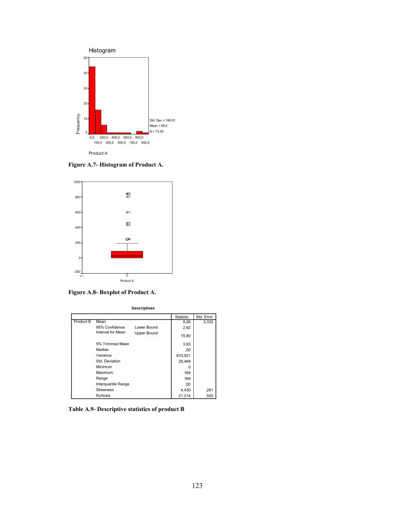
123
Product A
900,0800,0
700,0600,0
500,0400,0
300,0200,0
100,00,0
Histogram
Freq
uenc
y
50
40
30
20
10
0
Std. Dev = 186,91 Mean = 98,0
N = 73,00
Figure A.7- Histogram of Product A.
73N =
Product A
1000
800
600
400
200
0
-200
5049
5859
13
575414
Figure A.8- Boxplot of Product A.
Descriptives
9,26 3,3322,62
15,90
3,93,00
810,50128,469
0169169,00
4,430 ,28121,214 ,555
MeanLower BoundUpper Bound
95% ConfidenceInterval for Mean
5% Trimmed MeanMedianVarianceStd. DeviationMinimumMaximumRangeInterquartile RangeSkewnessKurtosis
Product BStatistic Std. Error
Table A.9- Descriptive statistics of product B

124
Tests of Normality
,408 73 ,000 ,369 73 ,000Product BStatistic df Sig. Statistic df Sig.
Kolmogorov-Smirnova Shapiro-Wilk
Lilliefors Significance Correctiona.
Table A.10- Normality test of product B.
Product B
175,0150,0
125,0100,0
75,050,0
25,00,0
Histogram
Freq
uenc
y
70
60
50
40
30
20
10
0
Std. Dev = 28,47 Mean = 9,3
N = 73,00
Figure A.9- Histogram of Product B.
73N =
Product B
200
100
0
-100
4910532556596213
5830751
850
57
54
Figure A.10- Boxplot of Product B.
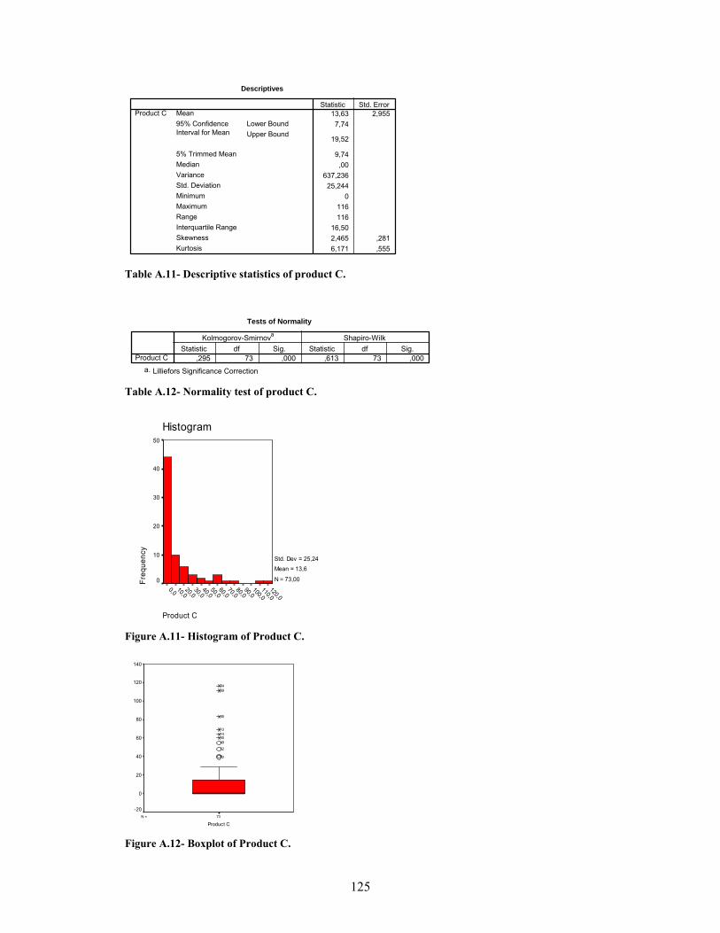
125
Descriptives
13,63 2,9557,74
19,52
9,74,00
637,23625,244
0116116
16,502,465 ,2816,171 ,555
MeanLower BoundUpper Bound
95% ConfidenceInterval for Mean
5% Trimmed MeanMedianVarianceStd. DeviationMinimumMaximumRangeInterquartile RangeSkewnessKurtosis
Product CStatistic Std. Error
Table A.11- Descriptive statistics of product C.
Tests of Normality
,295 73 ,000 ,613 73 ,000Product CStatistic df Sig. Statistic df Sig.
Kolmogorov-Smirnova Shapiro-Wilk
Lilliefors Significance Correctiona.
Table A.12- Normality test of product C.
Product C
120,0110,0
100,090,0
80,070,0
60,050,0
40,030,0
20,010,0
0,0
Histogram
Freq
uenc
y
50
40
30
20
10
0
Std. Dev = 25,24 Mean = 13,6
N = 73,00
Figure A.11- Histogram of Product C.
73N =
Product C
140
120
100
80
60
40
20
0
-20
126
52
49301413
35
5954
Figure A.12- Boxplot of Product C.

126
Descriptives
38,05 13,07212,00
64,11
18,541,00
12474,775111,691
0808808
23,505,213 ,281
32,336 ,555
MeanLower BoundUpper Bound
95% ConfidenceInterval for Mean
5% Trimmed MeanMedianVarianceStd. DeviationMinimumMaximumRangeInterquartile RangeSkewnessKurtosis
Product DStatistic Std. Error
Table A.13- Descriptive statistics of product D
Tests of Normality
,367 73 ,000 ,376 73 ,000Product DStatistic df Sig. Statistic df Sig.
Kolmogorov-Smirnova Shapiro-Wilk
Lilliefors Significance Correctiona.
Table A.14- Normality test of product D.
Product D
800,0700,0
600,0500,0
400,0300,0
200,0100,0
0,0
Histogram
Freq
uenc
y
70
60
50
40
30
20
10
0
Std. Dev = 111,69 Mean = 38,1
N = 73,00
Figure A.13- Histogram of Product D.

127
73N =
Product D
1000
800
600
400
200
0
-200
3130535013
44495437
58
57
Figure A.14- Boxplot of Product D.
Descriptives
5,11 1,8161,49
8,73
2,19,00
240,65415,513
08686
,004,080 ,281
17,837 ,555
MeanLower BoundUpper Bound
95% ConfidenceInterval for Mean
5% Trimmed MeanMedianVarianceStd. DeviationMinimumMaximumRangeInterquartile RangeSkewnessKurtosis
Product EStatistic Std. Error
Table A.15- Descriptive statistics of product E
Tests of Normality
,424 73 ,000 ,378 73 ,000Product EStatistic df Sig. Statistic df Sig.
Kolmogorov-Smirnova Shapiro-Wilk
Lilliefors Significance Correctiona.
Table A.16- Normality test of product E.
Product E
90,080,0
70,060,0
50,040,0
30,020,0
10,00,0
Histogram
Freq
uenc
y
70
60
50
40
30
20
10
0
Std. Dev = 15,51 Mean = 5,1
N = 73,00
Figure A.15- Histogram of Product E.

128
73N =
Product E
100
80
60
40
20
0
-20
145449474812565125
4
8
3010
5859
Figure A.16- Boxplot of Product E.
Descriptives
1,78 ,758,27
3,29
,49,00
41,9246,475
03535,00
3,878 ,28114,977 ,555
MeanLower BoundUpper Bound
95% ConfidenceInterval for Mean
5% Trimmed MeanMedianVarianceStd. DeviationMinimumMaximumRangeInterquartile RangeSkewnessKurtosis
Product FStatistic Std. Error
Table A.17- Descriptive statistics of product F
Tests of Normality
,526 73 ,000 ,306 73 ,000Product FStatistic df Sig. Statistic df Sig.
Kolmogorov-Smirnova Shapiro-Wilk
Lilliefors Significance Correctiona.
Table A.18- Normality test of product F
Product F
40,030,020,010,00,0
Histogram
Freq
uenc
y
80
70
60
50
40
30
20
10
0
Std. Dev = 6,47 Mean = 1,8
N = 73,00
Figure A.17- Histogram of Product F.

129
73N =
Product F
40
30
20
10
0
-10
50
14
5954
58
57
Figure A.18- Boxplot of Product F.

130
Case Calls Chemo pts Product_b packs_a packs_c packs_d packs_f packs_e Guidelines
1 3 129 0 60 0 2 0 0 122 5 277 0 28 2 4 0 0 83 70 546 0 20 0 6 0 0 484 159 979 0 189 26 8 0 24 1705 10 248 0 23 0 4 0 0 166 9 492 0 80 40 2 0 0 687 42 402 39 0 18 40 0 0 488 18 1445 60 56 0 42 0 30 489 15 651 0 43 13 20 0 0 16
10 138 1072 10 90 22 5 0 38 9211 15 320 0 32 20 10 0 0 4012 190 1356 0 0 39 0 0 10 17213 501 4745 16 600 69 96 0 0 37414 610 2955 0 850 64 4 15 2 53015 0 15 0 0 0 0 0 0 016 0 0 0 20 0 0 0 0 017 2 53 0 0 0 1 0 0 1218 0 35 0 0 0 0 0 0 019 0 6 0 0 0 0 0 0 020 0 42 0 0 0 0 0 0 021 0 360 0 36 0 1 0 0 022 4 97 0 2 0 0 0 0 1023 0 0 0 2 0 0 0 0 024 0 0 0 2 0 0 0 0 025 114 566 11 90 12 29 0 18 7826 41 210 0 35 4 2 0 0 2827 4 0 0 8 0 2 0 0 1228 3 0 0 11 0 0 0 0 029 2 275 0 30 0 0 0 0 1030 157 760 34 158 60 65 0 36 12831 14 0 0 16 13 59 0 0 1632 2 151 0 0 0 0 0 0 833 2 11 0 30 5 0 0 0 434 25 1221 0 20 29 0 0 0 6435 11 783 0 160 83 30 0 0 4036 49 167 0 60 0 0 0 0 5237 159 889 0 120 7 260 0 0 17238 10 155 0 36 0 0 0 0 2039 16 470 0 82 3 12 0 0 5240 4 198 0 1 0 0 0 0 441 42 1652 0 60 10 12 0 0 7642 7 845 0 75 6 0 0 0 1643 2 229 0 18 0 0 0 0 844 99 1397 0 120 24 170 0 0 6645 4 900 0 2 0 0 0 0 1646 18 366 0 94 3 14 0 0 2447 11 842 0 100 0 0 0 4 1648 8 186 0 21 6 27 0 9 1649 308 452 5 251 55 210 0 4 19250 48 602 60 245 0 80 10 0 13651 17 53 39 44 0 48 0 14 3852 173 408 0 180 48 30 0 0 15253 63 1203 10 112 8 80 0 0 4654 375 3790 169 834 116 220 20 4 44855 104 239 0 160 12 0 0 0 6856 13 146 12 60 0 14 0 12 2457 716 2273 150 800 23 808 35 0 43658 319 1562 31 432 15 349 30 82 33859 525 1480 15 460 111 10 20 86 49860 1 289 0 16 0 0 0 0 261 0 0 0 1 0 0 0 0 062 60 494 15 75 29 2 0 0 7663 0 0 0 4 0 0 0 0 064 0 0 0 0 0 0 0 0 065 0 0 0 0 0 0 0 0 066 0 0 0 0 0 0 0 0 067 0 6 0 0 0 0 0 0 068 0 0 0 0 0 0 0 0 069 0 0 0 0 0 0 0 0 070 0 0 0 0 0 0 0 0 071 0 0 0 0 0 0 0 0 072 0 0 0 0 0 0 0 0 073 0 0 0 0 0 0 0 0 0
Table A.19- Original values in the dataset

131
APPENDIX B ______________________________________________________________________
Figure B.1- Dendrogram using Single Linkage method applied to standardized data

132
KMO and Bartlett's Test
,679
401,74336
,000
Kaiser-Meyer-Olkin Measure of SamplingAdequacy.
Approx. Chi-SquaredfSig.
Bartlett's Test ofSphericity
Table B.1 – Factor Analysis and Bartlett’s test excluding outliers
Anti-image Matrices
9,184E-02 7,532E-02 4,502E-02 -2,33E-02 7,975E-03 -6,46E-02 5,764E-02 -5,67E-02 -7,023E-027,532E-02 ,529 -8,39E-04 -2,93E-02 -1,74E-02 -5,89E-02 8,483E-02 -8,53E-02 -9,083E-024,502E-02 -8,39E-04 ,372 3,012E-02 -3,06E-02 -,143 -,183 -,253 -1,655E-02
-2,335E-02 -2,93E-02 3,012E-02 ,282 -,137 -8,51E-02 -,141 -3,81E-02 -6,243E-037,975E-03 -1,74E-02 -3,06E-02 -,137 ,446 8,192E-02 ,145 4,267E-02 -4,453E-02
-6,461E-02 -5,89E-02 -,143 -8,51E-02 8,192E-02 ,459 7,016E-02 ,180 8,059E-035,764E-02 8,483E-02 -,183 -,141 ,145 7,016E-02 ,347 ,138 -6,611E-02
-5,669E-02 -8,53E-02 -,253 -3,81E-02 4,267E-02 ,180 ,138 ,406 1,226E-02-7,023E-02 -9,08E-02 -1,66E-02 -6,24E-03 -4,45E-02 8,059E-03 -6,61E-02 1,226E-02 7,969E-02
,686a ,342 ,243 -,145 3,938E-02 -,315 ,323 -,294 -,821,342 ,772a -1,89E-03 -7,59E-02 -3,58E-02 -,120 ,198 -,184 -,442,243 -1,89E-03 ,503a 9,291E-02 -7,50E-02 -,346 -,508 -,650 -9,608E-02
-,145 -7,59E-02 9,291E-02 ,837a -,387 -,237 -,451 -,113 -4,163E-023,938E-02 -3,58E-02 -7,50E-02 -,387 ,800a ,181 ,369 ,100 -,236
-,315 -,120 -,346 -,237 ,181 ,726a ,176 ,418 4,215E-02,323 ,198 -,508 -,451 ,369 ,176 ,340a ,368 -,397
-,294 -,184 -,650 -,113 ,100 ,418 ,368 ,523a 6,814E-02-,821 -,442 -9,61E-02 -4,16E-02 -,236 4,215E-02 -,397 6,814E-02 ,724a
Total CallsPatients (anual)Product BProduct AProduct CProduct DProduct FProduct ETotal GuidelineTotal CallsPatients (anual)Product BProduct AProduct CProduct DProduct FProduct ETotal Guideline
Anti-image Covariance
Anti-image Correlation
Total CallsPatients(anual) Product B Product A Product C Product D Product F Product E
TotalGuideline
Measures of Sampling Adequacy(MSA)a.
Table B.2- Factor Analysis anti-image matrices excluding outliers
Anti-image Matrices
,103 7,115E-02 ,113 1,018E-04 -2,09E-02 -8,79E-02 -,103 -7,856E-027,115E-02 ,550 6,141E-02 6,708E-03 -6,38E-02 -8,17E-02 -,143 -9,231E-02
,113 6,141E-02 ,502 -7,45E-02 7,153E-02 -,148 -,281 -8,215E-021,018E-04 6,708E-03 -7,45E-02 ,354 -,114 -7,33E-02 2,607E-02 -4,933E-02
-2,088E-02 -6,38E-02 7,153E-02 -,114 ,517 6,278E-02 -2,03E-02 -2,317E-02-8,786E-02 -8,17E-02 -,148 -7,33E-02 6,278E-02 ,473 ,182 2,625E-02
-,103 -,143 -,281 2,607E-02 -2,03E-02 ,182 ,469 5,296E-02-7,856E-02 -9,23E-02 -8,22E-02 -4,93E-02 -2,32E-02 2,625E-02 5,296E-02 9,464E-02
,651a ,299 ,500 5,341E-04 -9,07E-02 -,399 -,469 -,798,299 ,781a ,117 1,519E-02 -,120 -,160 -,282 -,404,500 ,117 ,407a -,177 ,140 -,303 -,578 -,377
5,341E-04 1,519E-02 -,177 ,912a -,266 -,179 6,393E-02 -,269-9,072E-02 -,120 ,140 -,266 ,917a ,127 -4,12E-02 -,105
-,399 -,160 -,303 -,179 ,127 ,738a ,386 ,124-,469 -,282 -,578 6,393E-02 -4,12E-02 ,386 ,531a ,251-,798 -,404 -,377 -,269 -,105 ,124 ,251 ,719a
Total CallsPatients (anual)Product BProduct AProduct CProduct DProduct ETotal GuidelineTotal CallsPatients (anual)Product BProduct AProduct CProduct DProduct ETotal Guideline
Anti-image Covariance
Anti-image Correlation
Total CallsPatients(anual) Product B Product A Product C Product D Product E
TotalGuideline
Measures of Sampling Adequacy(MSA)a.
Table B.3- Factor Analysis anti-image matrices excluding outliers and product F

133
Correlations
1 -,015 -,029, ,897 ,805
73 73 73-,015 1 -,061,897 , ,609
73 73 73-,029 -,061 1,805 ,609 ,
73 73 73
Pearson CorrelationSig. (2-tailed)NPearson CorrelationSig. (2-tailed)NPearson CorrelationSig. (2-tailed)N
BART factor score 1for analysis PAF 3
BART factor score 2for analysis PAF 3
BART factor score 3for analysis PAF 3
BART factorscore 1 foranalysis PAF
3
BART factorscore 2 for
analysis PAF 3
BART factorscore 3 for
analysis PAF 3
Table B.4- Bartlett’s computed factor scores obtained with PAF
Correlations
1 ,000 ,000, 1,000 1,000
73 73 73,000 1 ,000
1,000 , 1,00073 73 73
,000 ,000 11,000 1,000 ,
73 73 73
Pearson CorrelationSig. (2-tailed)NPearson CorrelationSig. (2-tailed)NPearson CorrelationSig. (2-tailed)N
BART factor score 1 for analysis 1
BART factor score 2 for analysis 1
BART factor score 3 for analysis 1
BART factorscore 1 foranalysis 1
BART factorscore 2 foranalysis 1
BART factorscore 3 foranalysis 1
Table B.5- Bartlett’s computed factor scores obtained with PCF We can see that only in the PCF method the factors scores are uncorrelated.
Correlations
1 ,000 ,000, 1,000 1,000
73 73 73,000 1 ,000
1,000 , 1,00073 73 73
,000 ,000 11,000 1,000 ,
73 73 73
Pearson CorrelationSig. (2-tailed)NPearson CorrelationSig. (2-tailed)NPearson CorrelationSig. (2-tailed)N
A-R factor score 1for analysis PAF 4
A-R factor score 2for analysis PAF 4
A-R factor score 3for analysis PAF 4
A-R factorscore 1 for
analysisPAF 4
A-R factorscore 2 for
analysisPAF 4
A-R factorscore 3 for
analysisPAF 4
Table B.6- Anderson-Rubin computed factor scores obtained with PAF
We can use Anderson-Rubin Scores in the PAF method instead of Bartlett’s because they
proceed in the same manner as Bartlett except they added the condition that the factor scores are

134
required to be orthogonal (see table B.6), the disadvantage is that we may be adding a biasing
effect to our computed scores.
Factor Matrixa
,941 -,101,805 -,256,699 ,306,973 -9,05E-02,697 -,432,720 ,572,831 ,323,967 -,211
Total CallsPatients (anual)Product BProduct AProduct CProduct DProduct FTotal Guideline
1 2Factor
Extraction Method: Principal Axis Factoring.2 factors extracted. 14 iterations required.a.
Table B.7- PAF Factor Matrix for two factor extraction (excluding Product E).
Rotated Factor Matrixa
,783 ,530,780 ,324,336 ,685,802 ,559,811 ,120,181 ,901,426 ,784,875 ,463
Total CallsPatients (anual)Product BProduct AProduct CProduct DProduct FTotal Guideline
1 2Factor
Extraction Method: Principal Axis Factoring. Rotation Method: Varimax with Kaiser Normalization.
Rotation converged in 3 iterations.a.
Table B.8- PAF Varimax Rotation Factor Matrix for two factor extraction (excluding Product E).

135
Computation of random eigenvalues with Monte Carlo PCA for Parallel Analysis
Monte Carlo PCA for Parallel Analysis is a standalone RealBASIC program which allows
specification of 3-300 variables, 100- 2,500 participants, and 1-1,000 replications. The program:
(a) generates random normal data for the quantity of variables and participants selected; (b)
computes the correlation matrix; (c) calculates eigenvalues for those variables via a Jocobi
routine; (d) repeats the process as many times as specified in the replications field; and (e)
calculates the average and standard deviation of the eigenvalues across all replications1.
Bellow the calculated random eigenvalues used:
Monte Carlo PCA for Parallel Analysis ©2000 by Marley W. Watkins. All rights reserved. ******************************************************
0-09-2006 14:42:18 Number of variables: 9 Number of subjects: 73 Number of replications: 500 ++++++++++++++++++++++++++++++++++++++++++++++++++++++ Eigenvalue # Random Eigenvalue Standard Dev ++++++++++++++++++++++++++++++++++++++++++++++++++++++ 1 1,5878 ,1119 2 1,3777 ,0789 3 1,2201 ,0659 4 1,0897 ,0512 5 0,9692 ,0515 6 0,8559 ,0535 7 0,7443 ,0571 8 0,6369 ,0610 9 0,5183 ,0603 ++++++++++++++++++++++++++++++++++++++++++++++++++++++ 20-04-2007 14:42:20 Monte Carlo PCA for Parallel Analysis ©2000 by Marley W. Watkins. All rights reserved. ******************************************************
Freeware versions of Monte Carlo PCA for Parallel Analysis are available for Macintosh and
Windows operating systems at:
http://www.personal.psu.edu/mww10
1- Watkins M. (2006). Determining Parallel Analysis Criteria. Journal of Modern Applied
Statistical Methods 5: 344- 346.

136
Table B.9- Estmated Regression Coefficients (Sharma 1996)

137
CHCBCHCRHC CHC
HTV
CHAM
CHBA
CHBAR
CHMT
CHVG
CHVR
IPOC
IPOPORTO
IPOLX
AGUEDAHMPIAELVASSEIAPOMBALHSMADEIRALEIRIA
FAMALICÃOANADIAPENAFIELHASFF
CURRYESTEFÂNIAAVEIROBARCELOS
BARREIROBRAGANÇAALUSITANOCHAVES
EVORA
FARO
FIGUEIRAHGOGUARDA
GUIMARÃESMACEDO
BRAGA
SANTARÉM
SCACÉM
HSETÚBALHSFEIRAHVFXVISEU
PORTALEGRE
EGAS
HGSAHJU
HPV
HSFX
HSJOÃO
HSJ
HSCRUZ
HSMARIA
CAPUCHOS
HUC
STIRSOMAC
ULSM
HSTMARTAOVARHOAZOUTÃOMONTIJOESPINHOESTARREJAFAFELAGOSLAMEGOMIRANDELA
Figure B.2- 3 D Scatterplot using Bartlet factor scores calculated by PCA method We can see that the high value hospitals with atypical behaviour like IPO Porto, IPO Lisboa
(IPOLX), and H. São João load high in Factor 1 (Conventional), whereas we have Hospitais da
Universidade de Coimbra (HUC) and Capuchos that share the common characteristic of loading
highly in Factor 3 (Alternative). Hospital de Sta Maria main characteristic of loading high in
Factor 2 (Innovative) is also shown in the figure above.

138
APPENDIX C ______________________________________________________________________
Figure C.1- Dendrogram using Average Linkage (Between Groups) applied to all computed factor scores.

139
Figure C.2- Dendrogram using Centroid Method applied to all computed factor scores.
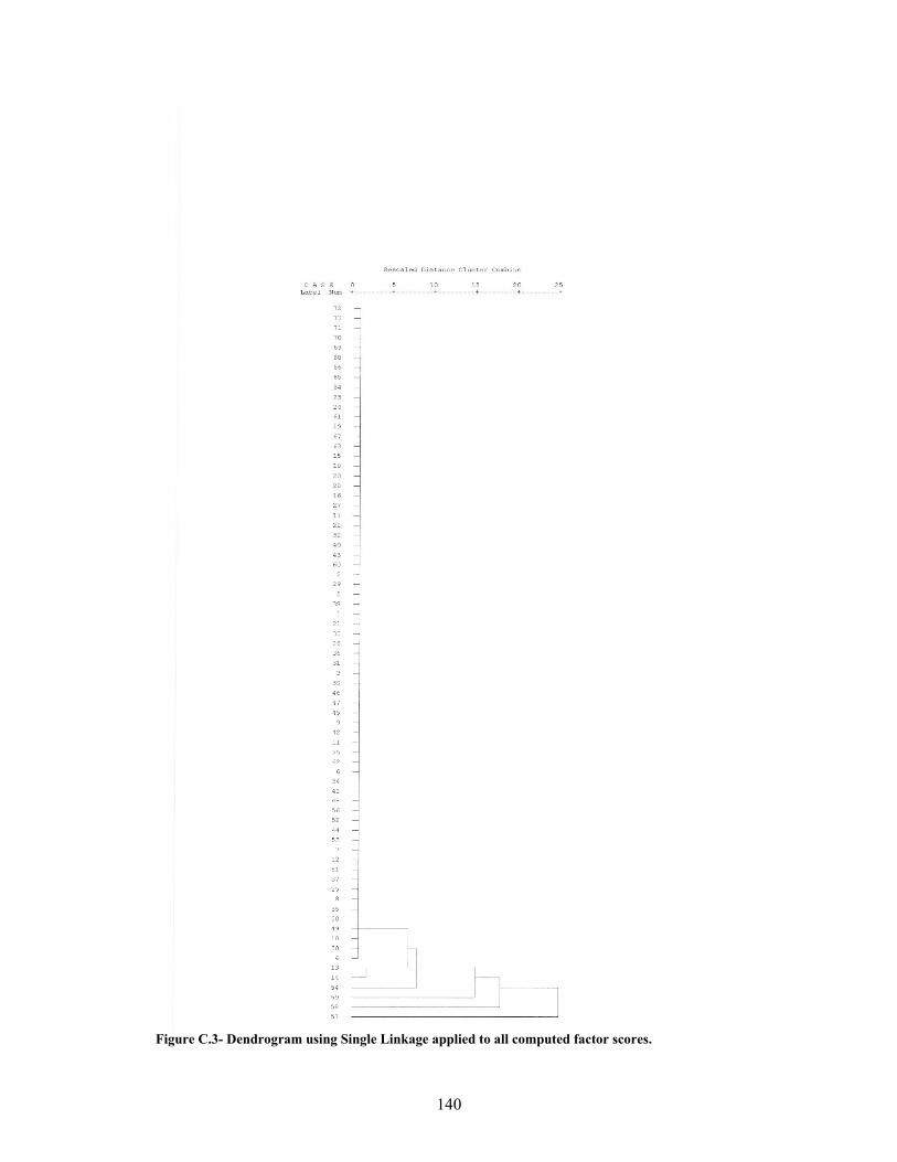
140
Figure C.3- Dendrogram using Single Linkage applied to all computed factor scores.
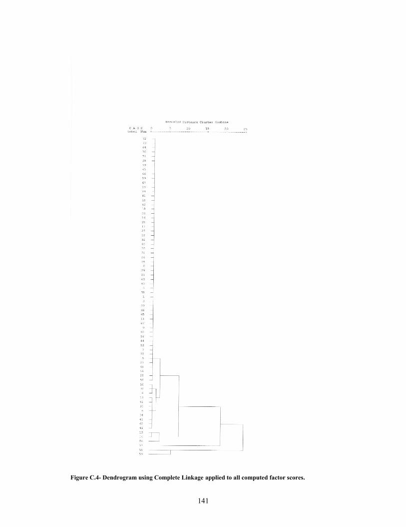
141
Figure C.4- Dendrogram using Complete Linkage applied to all computed factor scores.

142
Figure C.5- Dendrogram using Ward Method applied to all computed factor scores.

143
Table C.1- Mojena Values for the 5 agglomerative clustering methods Mojena
Number of clusters in the solution Ward Centroid Single Linkage Complete Linkage Average Linkage 72 -0,29 -0,27 -0,27 -0,25 -0,27 71 -0,29 -0,27 -0,27 -0,25 -0,27 70 -0,29 -0,27 -0,27 -0,25 -0,27 69 -0,29 -0,27 -0,27 -0,25 -0,27 68 -0,29 -0,27 -0,27 -0,25 -0,27 67 -0,29 -0,27 -0,27 -0,25 -0,27 66 -0,29 -0,27 -0,27 -0,25 -0,27 65 -0,29 -0,27 -0,27 -0,25 -0,27 64 -0,29 -0,27 -0,27 -0,25 -0,27 63 -0,29 -0,27 -0,27 -0,25 -0,27 62 -0,29 -0,27 -0,27 -0,25 -0,27 61 -0,29 -0,27 -0,27 -0,25 -0,27 60 -0,29 -0,27 -0,27 -0,25 -0,27 59 -0,29 -0,27 -0,27 -0,25 -0,27 58 -0,29 -0,27 -0,27 -0,25 -0,27 57 -0,29 -0,27 -0,27 -0,25 -0,27 56 -0,29 -0,27 -0,27 -0,25 -0,27 55 -0,29 -0,27 -0,27 -0,25 -0,27 54 -0,29 -0,27 -0,27 -0,25 -0,27 53 -0,29 -0,27 -0,27 -0,25 -0,27 52 -0,29 -0,27 -0,27 -0,25 -0,27 51 -0,29 -0,27 -0,27 -0,25 -0,27 50 -0,29 -0,27 -0,27 -0,25 -0,27 49 -0,29 -0,27 -0,27 -0,25 -0,27 48 -0,29 -0,27 -0,27 -0,25 -0,27 47 -0,29 -0,27 -0,27 -0,25 -0,27 46 -0,29 -0,27 -0,27 -0,25 -0,27 45 -0,29 -0,27 -0,27 -0,25 -0,27 44 -0,29 -0,27 -0,27 -0,25 -0,27 43 -0,29 -0,27 -0,27 -0,25 -0,27 42 -0,28 -0,27 -0,27 -0,25 -0,27 41 -0,28 -0,27 -0,27 -0,25 -0,27 40 -0,28 -0,27 -0,27 -0,25 -0,27 39 -0,28 -0,27 -0,27 -0,25 -0,27 38 -0,28 -0,27 -0,27 -0,25 -0,27 37 -0,28 -0,27 -0,26 -0,25 -0,27 36 -0,28 -0,27 -0,26 -0,25 -0,27 35 -0,28 -0,27 -0,26 -0,25 -0,27 34 -0,28 -0,27 -0,26 -0,25 -0,27 33 -0,28 -0,27 -0,26 -0,25 -0,27 32 -0,28 -0,27 -0,26 -0,24 -0,27 31 -0,28 -0,27 -0,26 -0,24 -0,27 30 -0,28 -0,26 -0,26 -0,24 -0,27 29 -0,28 -0,26 -0,26 -0,24 -0,27 28 -0,28 -0,26 -0,26 -0,24 -0,26 27 -0,27 -0,26 -0,26 -0,24 -0,26 26 -0,27 -0,26 -0,25 -0,24 -0,26 25 -0,26 -0,26 -0,25 -0,24 -0,26 24 -0,26 -0,25 -0,25 -0,23 -0,25 23 -0,25 -0,23 -0,25 -0,23 -0,24 22 -0,25 -0,23 -0,23 -0,23 -0,24 21 -0,24 -0,23 -0,22 -0,23 -0,23 20 -0,23 -0,23 -0,22 -0,22 -0,23 19 -0,23 -0,22 -0,22 -0,21 -0,23 18 -0,22 -0,22 -0,21 -0,21 -0,22 17 -0,21 -0,21 -0,20 -0,21 -0,21 16 -0,19 -0,21 -0,20 -0,20 -0,21 15 -0,17 -0,19 -0,20 -0,18 -0,20 14 -0,14 -0,18 -0,20 -0,18 -0,18 13 -0,10 -0,17 -0,20 -0,15 -0,16 12 -0,06 -0,16 -0,20 -0,13 -0,15 11 -0,02 -0,16 -0,19 -0,11 -0,12 10 0,06 -0,06 -0,14 -0,07 -0,02 9 0,18 0,01 -0,14 0,01 -0,01 8 0,37 0,10 -0,11 0,14 0,11 7 0,56 0,18 0,17 0,36 0,20 6 0,88 0,97 1,25 0,44 0,93 5 1,31 2,16 1,60 1,10 2,27 4 2,56 2,50 3,39 1,74 2,32 3 4,34 3,75 4,02 4,64 4,22 2 6,18 6,39 5,92 6,43 6,12
9,54 2,05 1,31 3,87 2,26
sα 33,43 7,61 4,92 15,60 8,28
_α

144
3 Cluster Solution 4 Cluster Solution 5 Cluster Solution 6 Cluster Solution
Case Average linkage
Complete linkage Ward Centroid Complete
linkage Single
Linkage Ward Average linkage Ward Complete
linkage Centroid Average linkage
Single Linkage Centroid
1 1 1 1 1 1 1 1 1 1 1 1 1 1 1 2 1 1 1 1 1 1 1 1 1 1 1 1 1 1 3 1 1 1 1 1 1 1 1 1 1 1 1 1 1 4 1 1 1 1 1 1 1 1 2 1 1 1 1 1 5 1 1 1 1 1 1 1 1 1 1 1 1 1 1 6 1 1 1 1 1 1 1 1 2 1 1 1 1 1 7 1 1 1 1 1 1 1 1 1 1 1 1 1 1 8 1 1 1 1 1 1 1 1 1 1 1 1 1 1 9 1 1 1 1 1 1 1 1 1 1 1 1 1 1 10 1 1 1 1 1 1 1 1 2 1 1 1 1 1 11 1 1 1 1 1 1 1 1 1 1 1 1 1 1 12 1 1 1 1 1 1 1 1 2 1 1 1 1 1 13 1 1 2 1 2 1 2 2 3 2 2 2 2 2 14 1 1 2 1 2 1 2 2 3 2 2 2 2 2 15 1 1 1 1 1 1 1 1 1 1 1 1 1 1 16 1 1 1 1 1 1 1 1 1 1 1 1 1 1 17 1 1 1 1 1 1 1 1 1 1 1 1 1 1 18 1 1 1 1 1 1 1 1 1 1 1 1 1 1 19 1 1 1 1 1 1 1 1 1 1 1 1 1 1 20 1 1 1 1 1 1 1 1 1 1 1 1 1 1 21 1 1 1 1 1 1 1 1 1 1 1 1 1 1 22 1 1 1 1 1 1 1 1 1 1 1 1 1 1 23 1 1 1 1 1 1 1 1 1 1 1 1 1 1 24 1 1 1 1 1 1 1 1 1 1 1 1 1 1 25 1 1 1 1 1 1 1 1 1 1 1 1 1 1 26 1 1 1 1 1 1 1 1 1 1 1 1 1 1 27 1 1 1 1 1 1 1 1 1 1 1 1 1 1 28 1 1 1 1 1 1 1 1 1 1 1 1 1 1 29 1 1 1 1 1 1 1 1 1 1 1 1 1 1 30 1 1 1 1 1 1 1 1 2 1 1 1 1 1 31 1 1 1 1 1 1 1 1 1 1 1 1 1 1 32 1 1 1 1 1 1 1 1 1 1 1 1 1 1 33 1 1 1 1 1 1 1 1 1 1 1 1 1 1 34 1 1 1 1 1 1 1 1 2 1 1 1 1 1 35 1 1 1 1 1 1 1 1 2 1 1 1 1 1 36 1 1 1 1 1 1 1 1 1 1 1 1 1 1 37 1 1 1 1 1 1 1 1 1 1 1 1 1 1 38 1 1 1 1 1 1 1 1 1 1 1 1 1 1 39 1 1 1 1 1 1 1 1 1 1 1 1 1 1 40 1 1 1 1 1 1 1 1 1 1 1 1 1 1 41 1 1 1 1 1 1 1 1 2 1 1 1 1 1 42 1 1 1 1 1 1 1 1 1 1 1 1 1 1 43 1 1 1 1 1 1 1 1 1 1 1 1 1 1 44 1 1 1 1 1 1 1 1 1 1 1 1 1 1 45 1 1 1 1 1 1 1 1 1 1 1 1 1 1 46 1 1 1 1 1 1 1 1 1 1 1 1 1 1 47 1 1 1 1 1 1 1 1 1 1 1 1 1 1 48 1 1 1 1 1 1 1 1 1 1 1 1 1 1 49 1 1 1 1 1 1 1 1 2 1 1 1 1 1 50 1 1 1 1 1 1 1 1 1 1 1 1 1 1 51 1 1 1 1 1 1 1 1 1 1 1 1 1 1 52 1 1 1 1 1 1 1 1 2 1 1 1 1 1 53 1 1 1 1 1 1 1 1 1 1 1 1 1 1 54 1 1 2 1 2 1 2 2 3 2 2 3 3 3 55 1 1 1 1 1 1 1 1 2 1 1 1 1 1 56 1 1 1 1 1 1 1 1 1 1 1 1 1 1 57 2 2 2 2 3 2 3 3 4 3 3 4 4 4 58 3 3 3 3 4 3 4 4 5 4 4 5 5 5 59 3 3 3 3 4 4 4 5 5 5 5 6 6 6 60 1 1 1 1 1 1 1 1 1 1 1 1 1 1 61 1 1 1 1 1 1 1 1 1 1 1 1 1 1 62 1 1 1 1 1 1 1 1 2 1 1 1 1 1 63 1 1 1 1 1 1 1 1 1 1 1 1 1 1 64 1 1 1 1 1 1 1 1 1 1 1 1 1 1 65 1 1 1 1 1 1 1 1 1 1 1 1 1 1 66 1 1 1 1 1 1 1 1 1 1 1 1 1 1 67 1 1 1 1 1 1 1 1 1 1 1 1 1 1 68 1 1 1 1 1 1 1 1 1 1 1 1 1 1 69 1 1 1 1 1 1 1 1 1 1 1 1 1 1 70 1 1 1 1 1 1 1 1 1 1 1 1 1 1 71 1 1 1 1 1 1 1 1 1 1 1 1 1 1 72 1 1 1 1 1 1 1 1 1 1 1 1 1 1 73 1 1 1 1 1 1 1 1 1 1 1 1 1 1
Table C.2- Cluster solutions for all methods including ward 5 clusters solution.

145
Block Distance
Figure C.6- Dendrogram using Average Linkage (Between Groups) with city block distance applied to all computed factor scores.
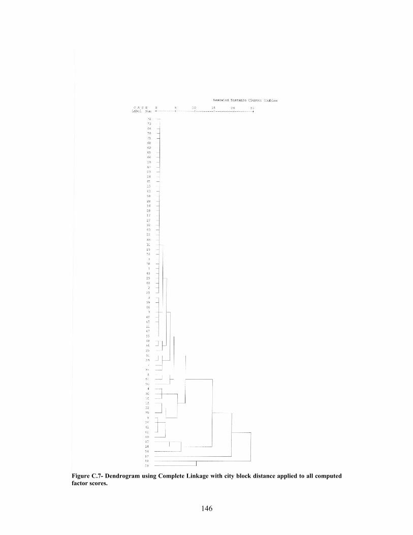
146
Figure C.7- Dendrogram using Complete Linkage with city block distance applied to all computed factor scores.

147
Figure C.8- Dendrogram using Single Linkage with city block distance applied to all computed factor scores.

148
Mojena
Number of clusters in the solution Single Linkage Complete Linkage Average Linkage 72 -0,46 -0,44 -0,49 71 -0,46 -0,44 -0,49 70 -0,46 -0,44 -0,49 69 -0,46 -0,44 -0,49 68 -0,46 -0,44 -0,49 67 -0,46 -0,44 -0,49 66 -0,46 -0,44 -0,49 65 -0,46 -0,44 -0,49 64 -0,46 -0,44 -0,49 63 -0,46 -0,44 -0,49 62 -0,46 -0,44 -0,49 61 -0,46 -0,44 -0,49 60 -0,46 -0,44 -0,49 59 -0,46 -0,44 -0,49 58 -0,46 -0,43 -0,48 57 -0,45 -0,43 -0,48 56 -0,45 -0,43 -0,48 55 -0,45 -0,43 -0,47 54 -0,44 -0,42 -0,47 53 -0,44 -0,42 -0,47 52 -0,44 -0,42 -0,47 51 -0,44 -0,42 -0,47 50 -0,43 -0,42 -0,47 49 -0,43 -0,42 -0,46 48 -0,43 -0,42 -0,46 47 -0,43 -0,42 -0,46 46 -0,43 -0,42 -0,46 45 -0,43 -0,42 -0,46 44 -0,43 -0,41 -0,46 43 -0,43 -0,41 -0,46 42 -0,42 -0,40 -0,44 41 -0,42 -0,39 -0,43 40 -0,42 -0,39 -0,42 39 -0,40 -0,39 -0,42 38 -0,38 -0,37 -0,42 37 -0,37 -0,36 -0,38 36 -0,35 -0,36 -0,38 35 -0,35 -0,35 -0,37 34 -0,33 -0,34 -0,36 33 -0,33 -0,33 -0,35 32 -0,32 -0,33 -0,34 31 -0,32 -0,31 -0,33 30 -0,28 -0,31 -0,31 29 -0,27 -0,30 -0,29 28 -0,26 -0,27 -0,29 27 -0,20 -0,26 -0,28 26 -0,20 -0,24 -0,22 25 -0,19 -0,21 -0,18 24 -0,13 -0,17 -0,13 23 -0,11 -0,16 -0,08 22 -0,09 -0,15 -0,06 21 -0,01 -0,14 -0,05 20 -0,01 -0,09 -0,05 19 0,02 -0,08 -0,03 18 0,08 -0,04 0,06 17 0,09 0,01 0,08 16 0,11 0,01 0,10 15 0,12 0,14 0,22 14 0,14 0,17 0,22 13 0,14 0,23 0,32 12 0,19 0,33 0,33 11 0,20 0,35 0,46 10 0,25 0,39 0,59 9 0,36 0,66 0,68 8 0,51 0,88 0,73 7 1,08 1,12 1,12 6 1,91 1,32 1,83 5 2,51 1,99 2,96 4 3,90 2,99 3,23 3 4,19 4,07 4,17 2 4,27 5,39 4,30
0,64 0,64 0,89 sα 1,39 1,39 1,82
Table C.3- Mojena values for the 3 linkage methods using city block distance
_α
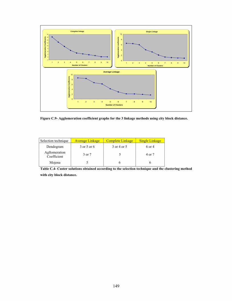
149
Complete linkage
0
2
4
6
8
10
12
14
16
18
10987654321
Number of Clusters
Agg
lom
erat
ion
Coe
ffici
ents
Single Linkage
0
2
4
6
8
10
10987654321Number of Clusters
Agg
lom
erat
ion
coef
ficie
nts
Average Linkage
0
2
4
6
8
10
10987654321
Number of Clusters
Agg
lom
erat
ion
Coe
ffici
ents
Figure C.9- Agglomeration coefficient graphs for the 3 linkage methods using city block distance.
Selection technique Average Linkage Complete Linkage Single Linkage
Dendogram 3 or 5 or 6 3 or 4 or 5 6 or 4 Agllomeration
Coefficient 3 or 7 5 4 or 7
Mojena 5 6 6
Table C.4- Custer solutions obtained according to the selection technique and the clustering method
with city block distance.

150
3 Cluster Solution 4 Cluster Solution 5 Cluster Solution 6 Cluster Solution 7 Cluster Solution
Case Average linkage
Complete linkage
Complete linkage
Single Linkage
Average linkage
Complete linkage
Average linkage
Single Linkage
Complete linkage
Single Linkage
Average linkage
1 1 1 1 1 1 1 1 1 1 1 12 1 1 1 1 1 1 1 1 1 1 13 1 1 1 1 1 1 1 1 1 1 14 1 1 1 1 1 1 1 1 2 1 25 1 1 1 1 1 1 1 1 1 1 16 1 1 1 1 1 1 1 1 2 1 17 1 1 1 1 1 1 1 1 1 1 18 1 1 1 1 1 1 1 1 1 1 19 1 1 1 1 1 1 1 1 1 1 110 1 1 1 1 1 1 1 1 2 1 211 1 1 1 1 1 1 1 1 1 1 112 1 1 1 1 1 1 1 1 2 1 113 1 1 2 1 2 2 2 2 3 2 314 1 1 2 1 2 2 2 2 3 3 315 1 1 1 1 1 1 1 1 1 1 116 1 1 1 1 1 1 1 1 1 1 117 1 1 1 1 1 1 1 1 1 1 118 1 1 1 1 1 1 1 1 1 1 119 1 1 1 1 1 1 1 1 1 1 120 1 1 1 1 1 1 1 1 1 1 121 1 1 1 1 1 1 1 1 1 1 122 1 1 1 1 1 1 1 1 1 1 123 1 1 1 1 1 1 1 1 1 1 124 1 1 1 1 1 1 1 1 1 1 125 1 1 1 1 1 1 1 1 1 1 126 1 1 1 1 1 1 1 1 1 1 127 1 1 1 1 1 1 1 1 1 1 128 1 1 1 1 1 1 1 1 1 1 129 1 1 1 1 1 1 1 1 1 1 130 1 1 1 1 1 1 1 1 2 1 231 1 1 1 1 1 1 1 1 1 1 132 1 1 1 1 1 1 1 1 1 1 133 1 1 1 1 1 1 1 1 1 1 134 1 1 1 1 1 1 1 1 2 1 135 1 1 1 1 1 1 1 1 2 1 136 1 1 1 1 1 1 1 1 1 1 137 1 1 1 1 1 1 1 1 1 1 138 1 1 1 1 1 1 1 1 1 1 139 1 1 1 1 1 1 1 1 1 1 140 1 1 1 1 1 1 1 1 1 1 141 1 1 1 1 1 1 1 1 2 1 142 1 1 1 1 1 1 1 1 1 1 143 1 1 1 1 1 1 1 1 1 1 144 1 1 1 1 1 1 1 1 1 1 145 1 1 1 1 1 1 1 1 1 1 146 1 1 1 1 1 1 1 1 1 1 147 1 1 1 1 1 1 1 1 1 1 148 1 1 1 1 1 1 1 1 1 1 149 1 1 1 1 1 1 1 1 2 1 150 1 1 1 1 1 1 1 1 1 1 151 1 1 1 1 1 1 1 1 1 1 152 1 1 1 1 1 1 1 1 2 1 153 1 1 1 1 1 1 1 1 1 1 154 1 1 2 1 2 2 3 3 3 4 455 1 1 1 1 1 1 1 1 1 1 156 1 1 1 1 1 1 1 1 1 1 157 2 2 3 2 3 3 4 4 4 5 558 3 3 4 3 4 4 5 5 5 6 659 3 3 4 4 5 5 6 6 6 7 760 1 1 1 1 1 1 1 1 1 1 161 1 1 1 1 1 1 1 1 1 1 162 1 1 1 1 1 1 1 1 2 1 163 1 1 1 1 1 1 1 1 1 1 164 1 1 1 1 1 1 1 1 1 1 165 1 1 1 1 1 1 1 1 1 1 166 1 1 1 1 1 1 1 1 1 1 167 1 1 1 1 1 1 1 1 1 1 168 1 1 1 1 1 1 1 1 1 1 169 1 1 1 1 1 1 1 1 1 1 170 1 1 1 1 1 1 1 1 1 1 171 1 1 1 1 1 1 1 1 1 1 172 1 1 1 1 1 1 1 1 1 1 173 1 1 1 1 1 1 1 1 1 1 1
Table C.5- Cluster solutions for all linkage methods using city block distance

151
Only the complete linkage method with 6 cluster solution produced a similar output to the ward
method but with the disadvantage of creating 3 individual clusters in the high value segment.
Figure C.10- Dendrogram using Average Linkage (Between Groups) excluding the outliers.

152
Figure C.11- Dendrogram using Complete Linkage excluding the outliers.

153
Figure C.12- Dendrogram using Single Linkage excluding the outliers.
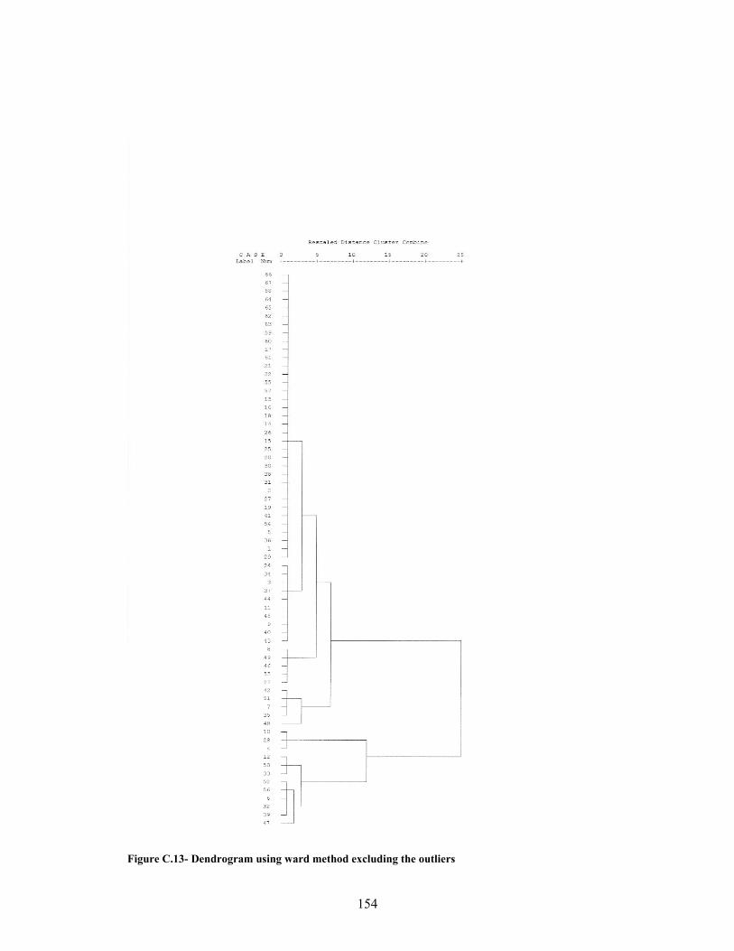
154
Figure C.13- Dendrogram using ward method excluding the outliers

155
Figure C.14 - Dendrogram using centroid method excluding the outliers

156
Mojena
Number of clusters in the solution Ward Centroid Single Linkage Complete Linkage Average Linkage 66 -0,34 -0,39 -0,54 -0,34 -0,39 65 -0,34 -0,39 -0,54 -0,34 -0,39 64 -0,34 -0,39 -0,54 -0,34 -0,39 63 -0,34 -0,39 -0,54 -0,34 -0,39 62 -0,34 -0,39 -0,54 -0,34 -0,39 61 -0,34 -0,39 -0,54 -0,34 -0,39 60 -0,34 -0,39 -0,54 -0,34 -0,39 59 -0,34 -0,39 -0,54 -0,34 -0,39 58 -0,34 -0,39 -0,54 -0,34 -0,39 57 -0,34 -0,39 -0,54 -0,34 -0,39 56 -0,34 -0,39 -0,54 -0,34 -0,39 55 -0,34 -0,39 -0,54 -0,34 -0,39 54 -0,34 -0,39 -0,54 -0,34 -0,39 53 -0,34 -0,39 -0,54 -0,34 -0,39 52 -0,34 -0,39 -0,54 -0,34 -0,39 51 -0,34 -0,39 -0,54 -0,34 -0,39 50 -0,34 -0,39 -0,54 -0,34 -0,39 49 -0,34 -0,39 -0,54 -0,34 -0,39 48 -0,34 -0,39 -0,54 -0,34 -0,39 47 -0,34 -0,39 -0,53 -0,34 -0,39 46 -0,34 -0,39 -0,53 -0,34 -0,39 45 -0,34 -0,39 -0,53 -0,34 -0,39 44 -0,34 -0,39 -0,53 -0,34 -0,39 43 -0,34 -0,39 -0,53 -0,34 -0,39 42 -0,34 -0,39 -0,53 -0,33 -0,39 41 -0,34 -0,39 -0,53 -0,33 -0,39 40 -0,34 -0,39 -0,53 -0,33 -0,39 39 -0,34 -0,39 -0,53 -0,33 -0,39 38 -0,34 -0,39 -0,53 -0,33 -0,39 37 -0,34 -0,39 -0,53 -0,33 -0,39 36 -0,34 -0,39 -0,53 -0,33 -0,39 35 -0,34 -0,38 -0,53 -0,33 -0,38 34 -0,34 -0,38 -0,52 -0,33 -0,38 33 -0,34 -0,38 -0,52 -0,33 -0,38 32 -0,34 -0,38 -0,50 -0,32 -0,38 31 -0,33 -0,36 -0,50 -0,32 -0,36 30 -0,33 -0,36 -0,47 -0,32 -0,36 29 -0,33 -0,35 -0,47 -0,32 -0,35 28 -0,32 -0,35 -0,46 -0,31 -0,35 27 -0,32 -0,35 -0,44 -0,31 -0,34 26 -0,31 -0,34 -0,44 -0,30 -0,34 25 -0,31 -0,33 -0,43 -0,30 -0,34 24 -0,30 -0,33 -0,39 -0,29 -0,33 23 -0,30 -0,31 -0,33 -0,28 -0,32 22 -0,28 -0,28 -0,32 -0,28 -0,27 21 -0,26 -0,25 -0,25 -0,28 -0,26 20 -0,23 -0,24 -0,20 -0,23 -0,26 19 -0,20 -0,21 -0,05 -0,22 -0,19 18 -0,17 -0,08 -0,05 -0,14 -0,08 17 -0,14 0,06 0,00 -0,12 0,02 16 -0,11 0,10 0,38 -0,11 0,03 15 -0,07 0,15 0,71 -0,11 0,07 14 -0,03 0,16 0,79 -0,07 0,10 13 0,02 0,19 0,79 0,03 0,14 12 0,07 0,25 1,17 0,04 0,26 11 0,13 0,33 1,25 0,08 0,33 10 0,23 0,39 1,35 0,17 0,39 9 0,36 0,62 1,41 0,38 0,45 8 0,59 0,82 1,45 0,41 0,72 7 0,82 0,88 1,48 0,70 0,95 6 1,05 1,02 1,49 0,85 1,14 5 1,54 1,04 1,58 1,54 1,42 4 2,28 2,36 3,00 2,37 2,61 3 3,48 4,40 3,05 3,75 4,22 2 6,13 5,38 4,10 6,01 5,33
1,89 0,23 0,09 0,50 0,27 sα 5,49 0,59 0,17 1,49 0,69
Table C.6- Mojena Values for the 5 agglomerative clustering methods excluding the outliers.
_α

157
Case Summaries
55 55 55 55 55 55 55 55 5516,27 268,76 4,20 31,91 2,62 16,85 ,18 1,58 20,40
895 14782 231 1755 144 927 10 87 112216,8% 35,6% 34,2% 24,5% 14,5% 33,4% 7,7% 23,3% 22,2%75,3% 75,3% 75,3% 75,3% 75,3% 75,3% 75,3% 75,3% 75,3%
159 1445 60 245 24 260 10 30 1720 0 0 0 0 0 0 0 0
31,359 367,405 13,359 45,669 5,533 44,203 1,348 5,311 32,80112 12 12 12 12 12 12 12 12
114,67 825,67 5,33 118,58 37,75 30,33 ,00 9,33 108,171376 9908 64 1423 453 364 0 112 1298
25,9% 23,9% 9,5% 19,9% 45,5% 13,1% ,0% 30,0% 25,7%16,4% 16,4% 16,4% 16,4% 16,4% 16,4% 16,4% 16,4% 16,4%
308 1652 34 251 83 210 0 38 1929 239 0 0 10 0 0 0 40
89,996 435,919 10,290 75,478 21,158 59,791 ,000 14,730 51,6953 3 3 3 3 3 3 3 3
495,33 3830,00 61,67 761,33 83,00 106,67 11,67 2,00 450,671486 11490 185 2284 249 320 35 6 1352
27,9% 27,7% 27,4% 31,9% 25,0% 11,5% 26,9% 1,6% 26,8%4,1% 4,1% 4,1% 4,1% 4,1% 4,1% 4,1% 4,1% 4,1%
610 4745 169 850 116 220 20 4 530375 2955 0 600 64 4 0 0 374
117,602 895,670 93,297 139,948 28,688 108,394 10,408 2,000 78,0341 1 1 1 1 1 1 1 1
716,00 2273,00 150,00 800,00 23,00 808,00 35,00 ,00 436,00716 2273 150 800 23 808 35 0 436
13,5% 5,5% 22,2% 11,2% 2,3% 29,1% 26,9% ,0% 8,6%1,4% 1,4% 1,4% 1,4% 1,4% 1,4% 1,4% 1,4% 1,4%
716 2273 150 800 23 808 35 0 436716 2273 150 800 23 808 35 0 436
, , , , , , , , ,2 2 2 2 2 2 2 2 2
422,00 1521,00 23,00 446,00 63,00 179,50 25,00 84,00 418,00844 3042 46 892 126 359 50 168 836
15,9% 7,3% 6,8% 12,5% 12,7% 12,9% 38,5% 45,0% 16,6%2,7% 2,7% 2,7% 2,7% 2,7% 2,7% 2,7% 2,7% 2,7%
525 1562 31 460 111 349 30 86 498319 1480 15 432 15 10 20 82 338
145,664 57,983 11,314 19,799 67,882 239,709 7,071 2,828 113,13773 73 73 73 73 73 73 73 73
72,84 568,42 9,26 98,00 13,63 38,05 1,78 5,11 69,105317 41495 676 7154 995 2778 130 373 5044
100,0% 100,0% 100,0% 100,0% 100,0% 100,0% 100,0% 100,0% 100,0%100,0% 100,0% 100,0% 100,0% 100,0% 100,0% 100,0% 100,0% 100,0%
716 4745 169 850 116 808 35 86 5300 0 0 0 0 0 0 0 0
148,185 860,832 28,469 186,906 25,244 111,691 6,475 15,513 122,252
NMeanSum% of Total Sum% of Total NMaximumMinimumStd. DeviationNMeanSum% of Total Sum% of Total NMaximumMinimumStd. DeviationNMeanSum% of Total Sum% of Total NMaximumMinimumStd. DeviationNMeanSum% of Total Sum% of Total NMaximumMinimumStd. DeviationNMeanSum% of Total Sum% of Total NMaximumMinimumStd. DeviationNMeanSum% of Total Sum% of Total NMaximumMinimumStd. Deviation
Ward Method1
2
3
4
5
Total
Total CallsPatients(anual) Product B Product A Product C Product D Product F Product E
TotalGuideline
Table C.7- Descriptive statistics of the 5 Cluster solution using Ward method
Case Summaries
44 44 44 44 44 44 44 44 447,14 179,05 ,00 20,16 1,57 3,11 ,00 ,09 10,23314 7878 0 887 69 137 0 4 450
13,8% 31,9% ,0% 27,9% 11,6% 10,6% ,0% 2,0% 18,6%65,7% 65,7% 65,7% 65,7% 65,7% 65,7% 65,7% 65,7% 65,7%
0 0 0 0 0 0 0 0 070 900 0 100 20 59 0 4 52
14,031 249,237 ,000 27,349 4,117 9,616 ,000 ,603 14,3593 3 3 3 3 3 3 3 3
151,33 937,00 14,67 145,67 36,00 26,00 ,00 32,67 130,00454 2811 44 437 108 78 0 98 390
20,0% 11,4% 14,9% 13,8% 18,1% 6,0% ,0% 49,2% 16,1%4,5% 4,5% 4,5% 4,5% 4,5% 4,5% 4,5% 4,5% 4,5%
138 760 0 90 22 5 0 24 92159 1072 34 189 60 65 0 38 170
11,590 160,184 17,474 50,639 20,881 33,808 ,000 7,572 39,0389 9 9 9 9 9 9 9 9
102,44 788,56 2,22 109,56 38,33 31,78 ,00 1,56 100,89922 7097 20 986 345 286 0 14 908
40,6% 28,7% 6,8% 31,0% 57,8% 22,2% ,0% 7,0% 37,5%13,4% 13,4% 13,4% 13,4% 13,4% 13,4% 13,4% 13,4% 13,4%
9 239 0 0 10 0 0 0 40308 1652 15 251 83 210 0 10 192
102,131 498,671 5,069 82,617 22,472 67,974 ,000 3,432 55,2735 5 5 5 5 5 5 5 5
82,20 898,60 21,80 119,40 11,40 126,00 2,00 ,00 93,60411 4493 109 597 57 630 10 0 468
18,1% 18,2% 36,9% 18,8% 9,5% 48,8% 100,0% ,0% 19,3%7,5% 7,5% 7,5% 7,5% 7,5% 7,5% 7,5% 7,5% 7,5%
42 402 0 0 0 40 0 0 46159 1397 60 245 24 260 10 0 172
48,308 411,016 26,668 86,728 9,529 88,769 4,472 ,000 57,1216 6 6 6 6 6 6 6 6
28,33 401,83 20,33 45,17 3,00 26,67 ,00 13,83 34,00170 2411 122 271 18 160 0 83 204
7,5% 9,8% 41,4% 8,5% 3,0% 12,4% ,0% 41,7% 8,4%9,0% 9,0% 9,0% 9,0% 9,0% 9,0% 9,0% 9,0% 9,0%
0 15 0 0 0 0 0 0 0114 1445 60 90 12 48 0 30 78
42,486 547,450 24,105 31,537 5,020 17,705 ,000 9,968 27,30667 67 67 67 67 67 67 67 67
33,90 368,51 4,40 47,43 8,91 19,27 ,15 2,97 36,122271 24690 295 3178 597 1291 10 199 2420
100,0% 100,0% 100,0% 100,0% 100,0% 100,0% 100,0% 100,0% 100,0%100,0% 100,0% 100,0% 100,0% 100,0% 100,0% 100,0% 100,0% 100,0%
0 0 0 0 0 0 0 0 0308 1652 60 251 83 260 10 38 192
59,995 434,055 12,800 61,459 16,848 47,134 1,222 8,259 49,753
NMeanSum% of Total Sum% of Total NMinimumMaximumStd. DeviationNMeanSum% of Total Sum% of Total NMinimumMaximumStd. DeviationNMeanSum% of Total Sum% of Total NMinimumMaximumStd. DeviationNMeanSum% of Total Sum% of Total NMinimumMaximumStd. DeviationNMeanSum% of Total Sum% of Total NMinimumMaximumStd. DeviationNMeanSum% of Total Sum% of Total NMinimumMaximumStd. Deviation
Ward Method1
2
3
4
5
Total
Total CallsPatients(anual) Product B Product A Product C Product D Product F Product E
TotalGuideline
Table C.8- Descriptive statistics of the 5 Cluster solution using Ward method without outliers

158
APPENDIX D ______________________________________________________________________ SOMTOOLBOX MATLAB CODE %Variable Correlation analysis% sD=som_data_struct(data); sD=som_normalize(sD,'var'); sM=som_make(sD,'msize',[9 8]); %The values of components are denormalized so that the values shown on the color bar are in the original value range% som_show(sM,'comp',1:9,'norm','d'); ______________________________________________________________________ %Convert data to SOM sD=som_data_struct(data); %Initialize a map mapxsize=9; mapysize=8; sM=som_randinit(sD,'msize',[mapysize mapxsize],'rect','sheet'); sM.neigh='gaussian'; %Establish training parameters (1st phase) niterations_1=100; radius_ini_1=8; alpha_ini_1=0.5; %niterations_1=200 was also tested% %Establishing training parameters (2nd phase) niterations_2=200; radius_ini_2=4; alpha_ini_2= 0.2; %niterations_2=400 was also tested% sM1=som_seqtrain(sM,sD,'radius_ini',radius_ini_1,'radius_fin',1,'alpha_ini',alpha_ini_1,'trainlen',niterations_1, 'linear'); sM2=som_seqtrain(sM1,sD,'radius_ini',radius_ini_2,'radius_fin',1,'alpha_ini',alpha_ini_2,'trainlen',niterations_2,'linear'); %Obtain bmus, umat, hits sHits=som_hits(sM2,sD); [bmus,qerrors]=som_bmus(sM2,sD); sumat=som_umat(sM2); %error measures for sM2, given sD [qe,te]=som_quality(sM2,sD);

159
%Show Results som_show(sM2,'comp',1:3,'umat','all'); som_show_add('hit',sHits); % add labels to map structure% sM2 = som_label(sM2,'add',[1; 2; 3; 4; 5; 6; 7; 8; 9;], ['1'; '2';'3';'4';'5';'6';'7';'8';'9']); sM2 = som_label(sM2,'add',[10; 11; 12; 13; 14; 15; 16; 17; 18;], ['10'; '11';'12';'13';'14';'15';'16';'17';'18']); sM2 = som_label(sM2,'add',[19; 20; 21; 22; 23; 24; 25; 26; 27;], ['19'; '20';'21';'22';'23';'24';'25';'26';'27']); sM2 = som_label(sM2,'add',[28; 29; 30; 31; 32; 33; 34; 35; 36;], ['28'; '29';'30';'31';'32';'33';'34';'35';'36']); sM2 = som_label(sM2,'add',[37; 38; 39; 40; 41; 42; 43; 44; 45;], ['37'; '38';'39';'40';'41';'42';'43';'44';'45']); sM2 = som_label(sM2,'add',[46; 47; 48; 49; 50; 51; 52; 53; 54;], ['46'; '47';'48';'49';'50';'51';'52';'53';'54']); sM2 = som_label(sM2,'add',[55; 56; 57; 58; 59; 60; 61; 62; 63;], ['55'; '56';'57';'58';'59';'60';'61';'62';'63']); sM2 = som_label(sM2,'add',[64; 65; 66; 67; 68; 69; 70; 71; 72;], ['64'; '65';'66';'67';'68';'69';'70';'71';'72']); som_show_add('label',sM2);
Top Related