


Languages
Pages
Legal


Soliton Equations exhibiting“Pfaffian Solutions”
早大理工 広田良吾 (Ryogo Hirota)早大理工 岩尾昌央 (Masataka Iwao)阪大基礎工 辻本諭 (Satoshi Tujimoto)
Soliton equations whose solutions are expressed by pfaffians are briefly discussed. In-cluded are “Discrete-time Toda equation”, “Modified Toda equation of BKP type”, thecoupled modified $\mathrm{K}\mathrm{d}\mathrm{V}$ equation and (
$\zeta \mathrm{C}\mathrm{o}\mathrm{u}\mathrm{p}\mathrm{l}\mathrm{e}\mathrm{d}$ modified equation of derivative type”etc. The B\"acklund transformation of the discrete BKP equation in biliner form is de-scribed in detail in Appendix.
1 IntroductionPfaffian is known as a square root of an anti-symmetric determinant of order $2\mathrm{n}$ :
$\det|a_{jk}|_{1\leq j},k\leq 2n=[pf(a_{1}, a_{2}, \cdots, a2n)]^{2}$ .
We have, for example, for $\mathrm{n}=1$
$=pf(a_{1,2}a)2$ .
Hence$pf(a_{1}, a_{2})=a12$ .
For $\mathrm{n}=2$ ,
$=[a_{12}a_{34^{-}}a13a24+a_{14}a_{23}]2$ .
Hence$pf(a_{1}, a_{2}, a_{3}, a_{4})=a_{12}a_{34^{-a_{13^{O}}}}24+a_{14}a_{23}$ .
A square root of a determinant of a matrix $M$ of order $\mathrm{n}$ which is a sum of a unit matrix$E$ and a product of anti-symmetric matrices $A$ and $B$ is expressed by a two-componentpfaffian:
$\det|E+A\cross B|=[pf(a1, a2, \cdots, on’ b1, b2, \cdots, bn)]^{2}$ ,
数理解析研究所講究録1170巻 2000年 23-34 23
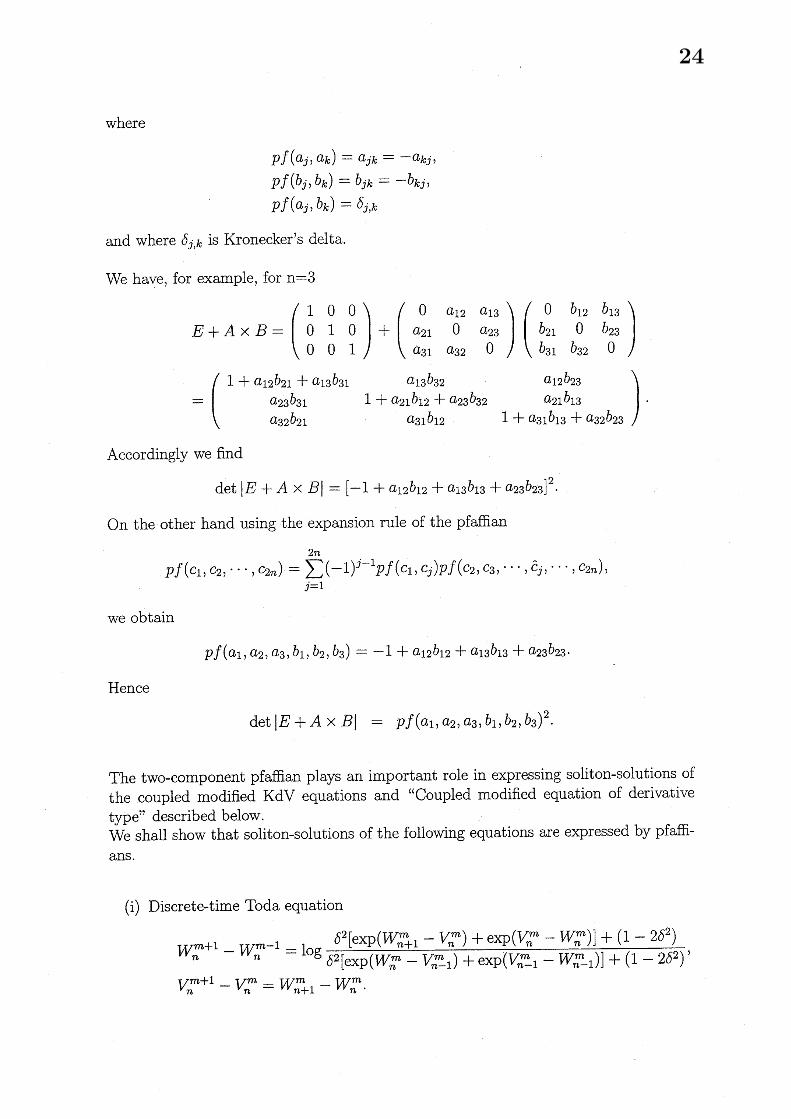
where
$pf(a_{j,k}a)=a_{j}k=-a_{kj}$ ,$pf(b_{j,k}b)=b_{jk}=-b_{k}j$ ,$pf(a_{j}, b_{k})=\delta_{j},k$
and where $\delta_{j,k}$ is Kronecker’s delta.
We have, for example, for $\mathrm{n}=3$
$E+A\cross B=+$$=$.
Accordingly we find
$\det|E+A\cross B|=[-1+a_{12}b_{12}+a_{13}b_{13}+a_{2\mathrm{s}^{b_{23}]^{2}}}$ .
On the other hand using the expansion rule of the pfaffian
$pf(C_{1}, C2, \cdots, c_{2n})=\sum_{j1}2n=(-1)j-1pf(c1, Cj)pf(C2, C3, \cdots,\hat{C}j)\ldots,2nc)$ ,
we obtain
$pf(a_{1}, a_{2,3}a, b_{1}, b2, b\mathrm{s})=-1+a12b_{12}+a_{13}b1\mathrm{s}+a23b_{23}$ .
Hence
$\det|E+\mathrm{A}\cross B|$ $=pf(a_{1}, a_{2,3,1,2,3}abbb)^{2}$ .
The two-component pfaffian plays an important role in expressing soliton-solutions of
the coupled modified $\mathrm{K}\mathrm{d}\mathrm{V}$ equations and “Coupled modified equation of derivativetype” described below.We shall show that soliton-solutions of the following equations are expressed by pfaffi-ans.
(i) Discrete-time Toda equation
$W_{n}^{m+1}-W_{n}m-1= \log\frac{\delta^{2}[\exp(Wm-V^{m})n+1n\mathrm{p}(+\mathrm{e}\mathrm{x}V_{n}^{m}-W_{n}m)]+(1-2\delta 2)}{\delta^{2}[\exp(Wm-nV_{n}^{m_{1}}-)+\exp(V_{n}m_{1^{-}}-W^{m}-1)n]+(1-2\delta^{2})}$ ,
$V_{n}^{m+1}-V^{m}=W_{n+1}nm-W^{m}n$ .
24

(ii) Modified Toda equation of BKP type
$\frac{d}{dt}\log\frac{\beta+V_{n}}{\beta-\alpha(In+I_{n-1})}=I_{n}-I_{n+1}$ ,
$\frac{d}{dt}I_{n}=V_{n-}1-V_{n}$ .
(iii) Coupled modified $\mathrm{K}\mathrm{d}\mathrm{V}$ equation
$\frac{\partial}{\partial t}v_{j}+6[\sum_{1\leq j<k\leq N}c_{j},kvjvk]\frac{\partial v_{j}}{\partial x}+\frac{\partial^{3}v_{j}}{\partial x^{3}}=0$ , $j=1,2,$ $\ldots,$$N$.
(iv) Coupled modified $\mathrm{K}\mathrm{d}\mathrm{V}$ equations of ($‘ \mathrm{d}\mathrm{e}\mathrm{r}\mathrm{i}\mathrm{v}\mathrm{a}\mathrm{t}\mathrm{i}\mathrm{v}\mathrm{e}$ type”
$\frac{\partial}{\partial t}v_{j}+6[\sum_{1\leq j<k\leq N}c_{j,k}D_{x}vj. v_{k}]\frac{\partial v_{j}}{\partial x}+\frac{\partial^{3}v_{j}}{\partial x^{3}}=0$ , $j=1,2,$ $\ldots,$$N$ .
We have the discrete KP equation
$[z_{1}\exp(D_{1})+z_{2}\exp(D2)+z_{\mathrm{s}}\exp(D3)]f\cdot f=0$
where $D_{1},$ $D_{2)}D_{3}$ and $z_{1},$ $z_{2,3}Z$ are bilinear operators and constants,respectively.Soliton solutions to the KP equation are known to be expressed by determinants [1].While the discrete BKP equation is expressed by
$[z_{1}\exp(D1)+z_{2}\exp(D2)+z_{3}\exp(D\mathrm{s})+z_{4}\exp(D_{4})]f\cdot f=0$
where $D_{1},$ $D_{2},$ $D_{3},$ $D_{4}$ and $z_{1},$ $z_{2},$ $Z_{3,4}Z$ are bilinear operators and constants, respectively,satisfying the relations
$D_{1}+D_{2}+D_{3}+D_{4}$ $=$ $0$ ,$z_{1}+z_{2}+Z3+z_{4}$ $=$ $0$ .
Solutions to the discrete BKP equation are well parametrized by parameters a,b and$\mathrm{c}$ which are the intervals of the coordinates $l,$ $m,$ $n[2]$ . We rewrite the discrete BKPequation using these parameters:
$(a+b)(a+c)(b-c)_{\mathcal{T}(\iota+1,m},$ $n)\mathcal{T}(l, m+1, n+1)$
$+(b+c)(b+a)(c-a)\mathcal{T}(\iota, m+1, n)\mathcal{T}(\iota+1, m, n+1)$
$+(C+a)(c+b)(a-b)_{\mathcal{T}}(\iota, m, n+1)_{\mathcal{T}}(l+1, m+1, n)$
$+(a-b)(b-c)(c-a)_{\mathcal{T}}(l, m, n)\tau(l+1, m+1, n+1)=0$.
Solutions are expressed by the pfaffian $[2],[3]$ :
$\tau(l, m, n)=pf(1,2,3, \cdots, 2N)$ ,
where the elements of the pfaffian are
$pf(j, k)\equiv cj,k$
$+ \sum_{\infty s=-}^{n-1}[\phi_{j(1}l, m, s+)\phi_{k}(l, m, S)-\phi_{j(}\iota, m, s)\phi k(\iota, m, S+1)]$
25
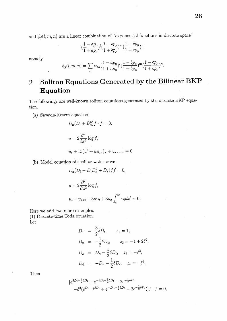
and $\phi_{j}(l, m, n)$ are a linear combination of (($\mathrm{e}\mathrm{x}\mathrm{p}\mathrm{o}\mathrm{n}\mathrm{e}\mathrm{n}\mathrm{t}\mathrm{i}\mathrm{a}\mathrm{l}$ functions in discrete space”
$( \frac{1-ap_{\mu}}{1+ap_{\mu}})^{l}(\frac{1-bp_{\mu}}{1+bp_{\mu}})^{m}(\frac{1-cp_{\mu}}{1+cp_{\mu}})^{n}$ ,
namely$\phi_{j}(l, m, n)=\sum_{\mu}\alpha_{j}\mu(\frac{1-ap_{\mu}}{1+ap_{\mu}})\iota(\frac{1-bp_{\mu}}{1+bp_{\mu}})^{m}(\frac{1-cp_{\mu}}{1+cp_{\mu}})^{n}$.
2 Soliton Equations Generated by the Bilinear BKPEquation
The followings are well-known soliton equations generated by the discrete BKP equa-tion.
(a) Sawada-Kotera equation
$D_{x}(D_{t}+D\overline{\mathrm{i})})xf\cdot f=0$,
$u=2 \frac{\partial^{2}}{\partial x^{2}}\log f$ ,
$u_{t}+15(u^{3}+uuxx)_{x}+u_{x}xxxx=0$ .
(b) Model equation of shallow-water wave
$D_{x}(D_{t}-D_{t}D_{x}^{2}+D_{x})f\dot{f}=0$ ,
$u=2 \frac{\partial^{2}}{\partial x^{2}}\log f$ ,
$u_{txt}-u_{x}-3uu_{t}+3u_{x} \int_{x}^{\infty}u_{t}dx’=0$ .
Here we add two more examples.(1) Discrete-time Toda equation.Let
$D_{1}$ $=$ $\frac{3}{2}\delta D_{t}$ , $z_{1}=1$ ,
$D_{2}$ $=$ $- \frac{1}{2}\delta D_{t}$ , $z_{2}=-1+2\delta 2$ ,
$D_{3}$ $=$ $D_{n}- \frac{1}{2}\delta D_{t}$ , $z_{\mathrm{s}=}-\delta^{2}$ ,
$D_{4}$ $=$ $-D_{nt}- \frac{1}{2}\delta D$ , $z_{4}=-\delta^{2}$ .
Then$[e^{\delta D_{t}+} \frac{1}{2}\delta D_{t}+e-\delta D_{t}+\frac{1}{2}\delta D_{t}-2e^{-}\frac{1}{2}\delta D_{t}$
$- \delta^{2}(e^{D_{n}\frac{1}{2}\delta D_{t}}-+e^{-D_{n}-}\frac{1}{2}\delta Dt-2e^{-}\frac{1}{2}\delta Di)]f\cdot f=0$,
26

which is rewritten as
$\cosh\frac{1}{2}\delta D_{t}[\sinh 2_{\frac{1}{2}}\delta Dt-\delta 2\sinh 2_{\frac{1}{2}}Dn]f\cdot f=0$ . (1)
The bilinear form indicates that 1-soliton solution is the same as that of the discrete-time Toda equation
$[\sinh^{2_{\frac{1}{2}\delta}}D_{t}-\delta^{2}\sinh^{2_{\frac{1}{2}}}D_{n}]f\cdot f=0$ .
The bilinear equation(l) is transformed into the nonlinear difference-difference equationin the ordinary form
$W_{n}^{m+1}-W_{n}^{m}-1= \log\frac{\delta^{2}[\exp(W_{n+1}^{m}+V^{m})n+\exp(V_{n}m-W_{n}^{m})]+(1-2\delta^{2})}{\delta^{2}[\exp(W^{m}+V_{n-}m)n1+\exp(V_{n}m_{1^{-}}-W^{m}-1)n]+(1-2\delta^{2})}$ ,
$V_{n}^{m+1m}-V_{n}m=WW_{n}^{m}n+1^{-}$’
through a series of dependent variable transformations
$f_{n}^{m}=e^{\phi^{m}}n$ ,$\triangle_{m}\phi^{m}n=\tau^{m}n$
’
$\triangle_{n}\phi_{n}^{m}=S_{n}^{m}$ ,$\triangle_{m}S_{n}^{m}=W_{n}m$ ,$\triangle_{n}S_{n}^{m}=V_{n}m$ ,
where $\triangle$ is the forward difference operator defined by
$\triangle_{m}f_{n}^{m}=\delta^{-1}[f_{n}^{m+1}-f_{n}^{m}]$ ,$\triangle_{n}f_{n}^{m}=fn+1m-fnm$ .
(2) Modified Toda equation of BKP type.Let
$D_{1}$ $=$ $\frac{1}{2}(\delta D_{x}+\epsilon D_{y})$ , $z_{1}=1$ ,
$D_{2}$ $=$ $\frac{1}{2}(\delta D_{x}-\epsilon D_{y})$ , $z_{2}=-1+\beta\delta\epsilon$ ,
$D_{3}$ $=$ $-D_{n}- \frac{1}{2}(\delta Dx+\epsilon D_{y})$ , $z_{3}=-\alpha\in-\beta\delta\epsilon$ ,
$D_{4}$ $=$ $D_{n}- \frac{1}{2}(\delta D_{x}-\epsilon D_{y})$ , $z_{4}=\alpha\epsilon$ .
Then
$\{e^{\frac{1}{2}(D_{x}+\epsilon D_{y}}\delta)-e\frac{1}{2}(\delta D_{x}-\epsilon D)y$
$+ \alpha\epsilon[e^{D_{n^{-}}(\delta}\frac{1}{2}D_{x^{-}}\epsilon D)-e^{-})yn^{-\frac{1}{2}(\delta DD_{y}}x+\epsilon]D$
$+ \beta\delta\epsilon[e^{\frac{1}{2}}-\epsilon D_{y}-(\delta Dx)e^{-D}\frac{1}{2}(\delta D_{x}+\epsilon D)v]n^{-}\}f\cdot f=0$ ,
27
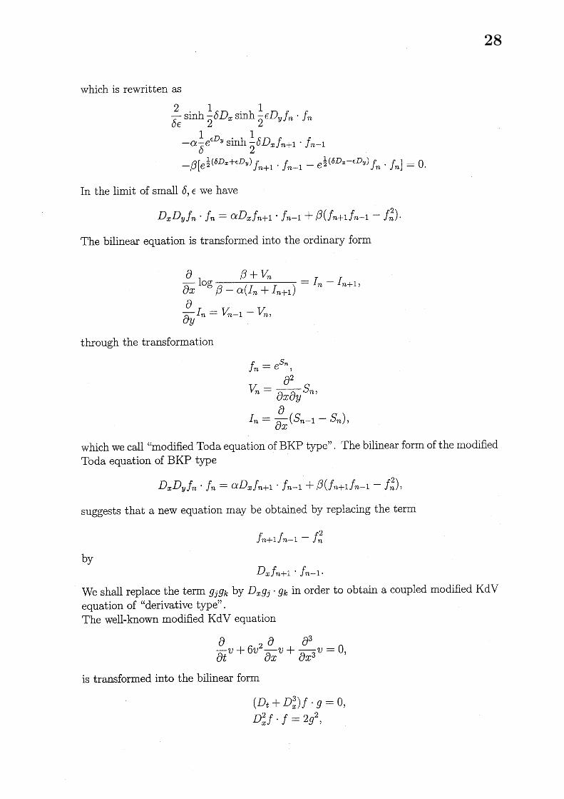
which is rewritten as
$\frac{2}{\delta\epsilon}\sinh\frac{1}{2}\delta D_{x}\sinh\frac{1}{2}\epsilon Dfyn$ . $f_{n}$
$- \alpha\frac{1}{\delta}e^{\epsilon}\mathrm{s}\mathrm{i}D_{y}\mathrm{n}\mathrm{h}\frac{1}{2}\delta Dxfn+1^{\cdot}fn-1$
$-\beta[e^{\frac{1}{2}()(\delta}\delta Dx+\epsilon Dyf_{n+1}\cdot fn-1-e^{\frac{1}{2}}fD_{x^{-}}\epsilon D_{y})n. f_{n}]=0$ .
In the limit of small $\delta,$ $\epsilon$ we have
$D_{x}D_{y}f_{n}\cdot fnx=\alpha Dfn+1^{\cdot}fn-1+\beta(f_{n}+1fn-1-f_{n}^{2})$ .
The bilinear equation is transformed into the ordinary form
$\frac{\partial}{\partial x}\log\frac{\beta+V_{n}}{\beta-\alpha(In+I_{n+1})}=I_{n}-I_{n+1}$,
$\frac{\partial}{\partial y}I_{n}=V_{n-}1-V_{n}$ ,
through the transformation
$f_{n}=e^{s_{n}}$ ,
$V_{n}= \frac{\partial^{2}}{\partial x\partial y}S_{n}$ ,
$I_{n}= \frac{\partial}{\partial x}(S_{n-}1^{-s)}n$
’
which we call “modified Toda equation of BKP type”. The bilinear form of the modifiedToda equation of BKP type
$D_{x}D_{y}f_{n}\cdot f_{n}=\alpha D_{x}f_{n+1}\cdot fn-1+\beta(f_{n}+1fn-1-f_{n}^{2})$ ,
suggests that a new equation may be obtained by replacing the term
$f_{n+1}f_{n-}1-f_{n}^{2}$
by$D_{x}f_{n+1}\cdot fn-1$ .
We shall replace the term $g_{j}g_{k}$ by $D_{x}g_{j}\cdot g_{k}$ in order to obtain a coupled modified $\mathrm{K}\mathrm{d}\mathrm{V}$
equation of ($‘ \mathrm{d}\mathrm{e}\mathrm{r}\mathrm{i}\mathrm{v}\mathrm{a}\mathrm{t}\mathrm{i}_{\mathrm{V}}\mathrm{e}$ type”.
The well-known modified $\mathrm{K}\mathrm{d}\mathrm{V}$ equation
$\frac{\partial}{\partial t}v+6v^{2_{\frac{\partial}{\partial x}v+}}\frac{\partial^{3}}{\partial x^{3}}v=0$ ,
is transformed into the bilinear form
$(D_{t}+D_{x}^{3})f\cdot \mathit{9}=0$ ,$D_{x}^{2}f\cdot f=2g^{2}$ ,
28
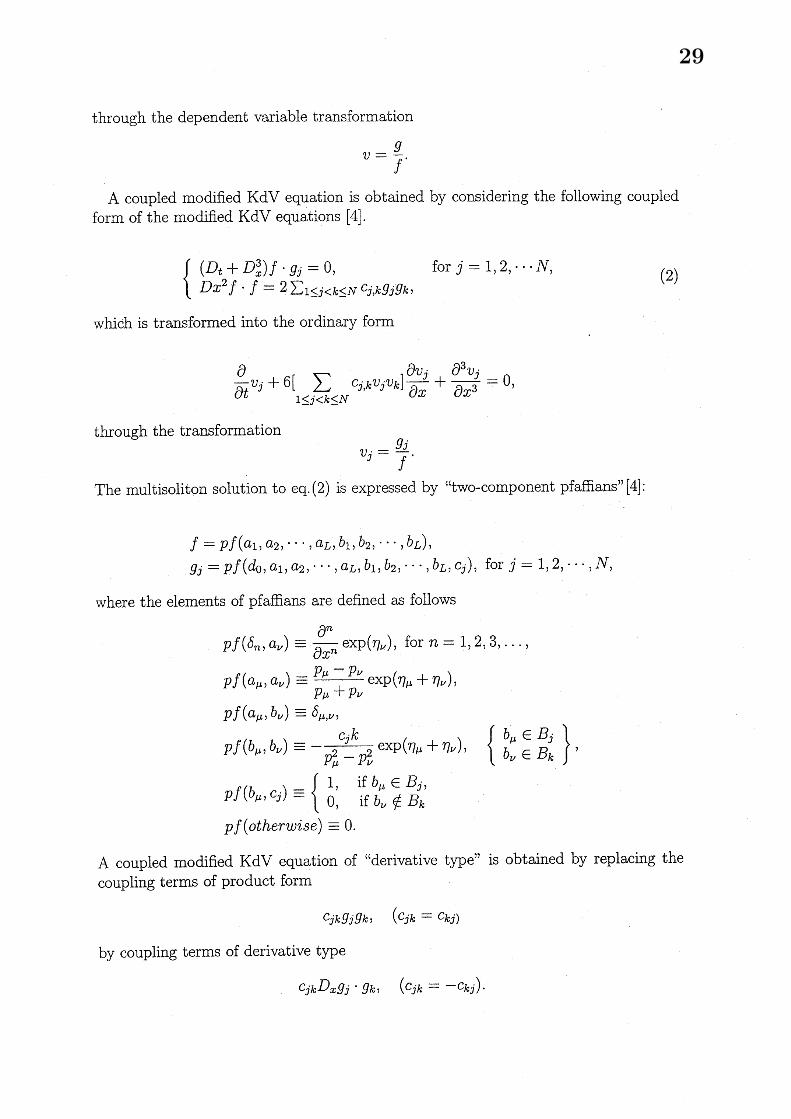
through the dependent variable transformation
$v= \frac{g}{f}$ .
A coupled modified $\mathrm{K}\mathrm{d}\mathrm{V}$ equation is obtained by considering the following coupledform of the modified $\mathrm{K}\mathrm{d}\mathrm{V}$ equations [4].
$\{$
$(D_{t}+D_{x}^{3})f\cdot g_{j}=0$ , for $j=1,2,$ $\cdots N$ , (2)$Dx^{2}f\cdot f=2\Sigma 1\leq j<k\leq NC_{j},k\mathit{9}jgk$ ,
which is transformed into the ordinary form
$\frac{\partial}{\partial t}v_{j}+6[1\leq j<\sum_{k\leq N}c_{j,k}vjv_{k}]\frac{\partial v_{j}}{\partial x}+\frac{\partial^{3}v_{j}}{\partial x^{3}}=0$,
through the transformation$v_{j}= \frac{g_{j}}{f}$ .
The multisoliton solution to $\mathrm{e}\mathrm{q}.(2)$ is expressed by ($‘ \mathrm{t}\mathrm{w}\mathrm{o}$-component pfaffians” [4]:
$f=pf(a_{1}, a2, \cdots, a_{L}, b1, b_{2}, \cdots, b_{L})$ ,$g_{j}=pf(d_{0}, a_{1}, a_{2}, \cdots, a_{L}, b_{1}, b_{2}, \cdot .., b_{L}, c_{j})$ , for $j=1,2,$ $\cdots,$
$N$,
where the elements of pfaffians are defined as follows
$pf( \delta_{n’ \mathcal{U}}a)\equiv\frac{\partial^{n}}{\partial x^{n}}\exp(\eta_{\nu})$ , for $n=1,2,3,$ $\ldots$ ,
$pf(a_{\mu’\nu}a) \equiv\frac{p_{\mu}-p_{\nu}}{p_{\mu}+p_{\nu}}\exp(\eta_{\mu}+\eta_{\nu})$ ,
$pf(a_{\mu}, b_{\mathcal{U}})\equiv\delta_{\mu},\nu$
’
$pf(b_{\mu’\nu}b) \equiv-\frac{c_{j}k}{p_{\mu}^{2}-p_{\nu}^{2}}\exp(\eta_{\mu}+\eta_{\overline{\nu}})$ ,
$pf(b_{\mu}, c_{j})\equiv\{$1, if $b_{\mu}\in B_{j}$ ,$0$ , if $b_{l\text{ノ}}\not\in B_{k}$
$pf(otherwi_{S}e)\equiv 0$ .
A coupled modified $\mathrm{K}\mathrm{d}\mathrm{V}$ equation of ($‘ \mathrm{d}\mathrm{e}\mathrm{r}\mathrm{i}\mathrm{v}\mathrm{a}\mathrm{t}\mathrm{i}\mathrm{v}\mathrm{e}$ type” is obtained by replacing the
coupling terms of product form
$c_{jk}g_{j}gk$ , $(cjk=ckj)$
by coupling terms of derivative type
$cjkDxgj.\mathit{9}k$ , $(_{C_{jk}}=-C_{k}j)$ .
29

We obtain
$\{$
$(D_{t}+D_{x}^{3})f\cdot g_{j}=0$ , for $j=1,2,$ $\cdots N$ ,$D_{x}^{2}f\cdot f=2\Sigma 1\leq j<k\leq NC_{j,x}kDgj$ .
$g_{k}$ ,(3)
which is transformed into the ordinary form
$\frac{\partial}{\partial t}v_{j}+6[\sum_{1\leq j<k\leq N}c_{j},k(D_{x}vj.v_{k})]\frac{\partial v_{j}}{\partial x}+\frac{\partial^{3}v_{j}}{\partial x^{3}}=0$ .
through the transformation$v_{j}= \frac{g_{j}}{f}$ .
The multisoliton solution to $\mathrm{e}\mathrm{q}.(3)$ is expressed by the same form as that of the coupledmodified $\mathrm{K}\mathrm{d}\mathrm{V}\cdot \mathrm{e}\mathrm{q}\mathrm{u}\mathrm{a}\mathrm{t}\mathrm{i}\mathrm{o}\mathrm{n}[5]$ :
$f=pf(a_{1}, a_{2}, \cdots, a_{L}, b1, b_{2}, \cdots, b_{L})$ ,$g_{j}=pf(d_{0,1}a, a2, \cdots, a_{L,1}b, b2, \cdots, bL, cj)$ , for $j=1,2,$ $\cdots,$
$N$ ,
where the elements of pfaffians are the same as those of the modified $\mathrm{K}\mathrm{d}\mathrm{V}$ equationexcept the element
$pf(b_{\mu’\nu}b) \equiv-\frac{c_{jk}}{p_{\mu}^{2}-p_{\nu}^{2}}\exp(\eta_{\mu}+\eta_{\nu})$, $)$ $(C_{jk}=Ckj)$ ,
is replaced by
$pf(b_{\mu}, b_{\nu}) \equiv-\frac{c_{jk}}{p_{\mu}+p_{\nu}}\exp(\eta_{\mu}+\eta_{\nu})$ ,
In conclusion we have shown that soliton-solutions of the following equations areexpressed by pfaffians.
(i) Discrete-time Toda equation
$W_{n}^{m+1}-W_{n}m-1= \log\frac{\delta^{2}[\exp(W_{n}mV+1^{-}nm)+\exp(V_{n}m-W_{n}m)]+(1-2\delta^{2})}{\delta^{2}[\exp(W^{m}-nV_{n-}m)1+\exp(V_{n}m_{1^{-}}-W^{m}-1)n]+(1-2\delta^{2})}$ ,
$V_{n}^{m+1}-V_{n}m=Wm-n+1W_{n}^{m}$ .
(ii) Modified Toda equation of BKP type
$\frac{d}{dt}\log\frac{\beta+V_{n}}{\beta-\alpha(In+I_{n-1})}=In-I_{n+1}$ ,
$\frac{d}{dt}I_{n}=V_{n}-1^{-}V_{n}$ .
(iii) Coupled modified $\mathrm{K}\mathrm{d}\mathrm{V}$ equation
$\frac{\partial}{\partial t}v_{j}+6[\sum_{1\leq j<k\leq N}c_{j,k}vjvk]\frac{\partial v_{j}}{\partial x}+\frac{\partial^{3}v_{j}}{\partial x^{3}}=0$ , $j=1,2,$ $\ldots,$$N$ .
(iv) Coupled modified equations of “derivative type”
$\frac{\partial}{\partial t}v_{j}+6[1\leq jk\leq N\sum_{<}cj,k\underline{Dxjv\cdot vk}]\frac{\partial v_{j}}{\partial x}+\frac{\partial^{3}v_{j}}{\partial x^{3}}=0$, $j=1,2,$ $\ldots,$$N$ .
30

AB\"acklund $\mathrm{n}\mathrm{a}\mathrm{n}\mathrm{S}\mathrm{f}\mathrm{o}\mathrm{r}\mathrm{m}\mathrm{a}\mathrm{t}\mathrm{i}_{\mathrm{o}\mathrm{n}}$ of the Discrete BKPEquation
In this appendix we describe in detail how to obtain the B\"acklund transformation ofthe discrete BKP equation in bilinear form.The B\"acklund transformation which relates a solution $f$ of the discrete BKP euqation
$[z_{1}\exp(D1)+z_{2}\exp(D2)+z_{3}\exp(D3)+z_{4}\exp(D4)]f\cdot f=0$
with another solution $f’$ of the same equation
$[z_{1}\exp(D_{1})+z_{2}\exp(D_{2})+Z_{3}\exp(D_{3})+z4\exp(D4)]f’\cdot f/=0$
is obtained by considering the following quantity $P$
$P=\{[z_{1}\exp(D1)+z_{2}\exp(D2)+z_{3}\exp(D3)+z_{4}\exp(D4)]f\cdot f\}$
$\cross\{[z_{3}\exp(D3)+z_{4}\exp(D_{4})]f’\cdot f’\}$
$-\{[z_{3}\exp(D3)+z_{4}\exp(D4)]f\cdot f\}$
$\cross\{[z_{1}\exp(D1)+Z_{2}\exp(D_{2})+Z3\exp(D_{3})+Z_{4}\exp(D_{4})]f/. f’\}$
$=0$
and using the exchange formula$(e^{D_{1}}f \cdot f)(e^{D\prime}f3. f’)=e^{\frac{1}{2}()}[D1+D_{3}e^{\frac{1}{2}(}D_{1}-D_{3})f\cdot f’]\cdot[e-\frac{1}{2}(D_{1}-D_{3})f\cdot f’]$. (4)
In fact we find
$(e^{D_{1}}f\cdot f)(eD3f’\cdot f’)-(eD1f’\cdot f’)(e^{D_{3}}f\cdot f)$
$=e^{\frac{1}{2}()} \{D_{1}+D_{3}[e^{\frac{1}{2}(D-D_{3}}f1). f’]\cdot[e-\frac{1}{2}(D_{1}-D_{3})f\cdot f’]-[e-\frac{1}{2}(D_{1}-D3)f\cdot f’]\cdot[e^{\frac{1}{2}(D_{3}}-)fD1\}$
$=2 \sinh\frac{1}{2}(D_{1}+D_{3})[e\frac{1}{2}(D1-D_{3})f\cdot f/]\cdot[e-\frac{1}{2}(D1-D_{3})f\cdot f/]$ . (5)
Using $\mathrm{e}\mathrm{q}(5)$ and noting that $D_{1}+D_{2}+D_{3}+D_{4}=0$ we rewrite $P$ as
$P=2_{Z_{13}}z \sinh\frac{1}{2}(D_{1}+D_{3})[e^{\frac{1}{2}}(D1-D_{3})f\cdot f’]\cdot[e^{-\frac{1}{2}(-}D_{1}D\mathrm{s})f\cdot f’]$
$-2z_{24}Z \sinh\frac{1}{2}(D_{1}+D_{3})[e^{\frac{1}{2}(-D_{4})}D2f\cdot f’]\cdot[e-\frac{1}{2}(D2-D_{4})f\cdot f’]$
$-2_{Z_{1^{Z}4}} \sinh\frac{1}{2}(D_{2}+D3)[e\frac{1}{2}(D_{1}-D_{4})f\cdot f/]\cdot[e^{-(D_{1}}\frac{1}{2}-D_{4})f\cdot f’]$
+2$Z_{2}Z3 \sinh\frac{1}{2}(D_{2}+D_{3})[e\frac{1}{2}(D2-D_{3})f\cdot f/]\cdot[e-\frac{1}{2}(D_{2}-D_{3})f\cdot f’]$
$=2 \sinh\frac{1}{2}(D_{1}+D_{3})$
$\{z_{1^{Z_{3}[}}e^{\frac{1}{2}}-D_{3})f(D_{1}$ . $f’$ ] $\cdot[e-\frac{1}{2}(D_{1}-D_{3})f\cdot f’]$
$-z_{2}z_{4}[e \frac{1}{2}(D_{2}-D_{4})f\cdot f’]\cdot[e-\frac{1}{2}(D_{2}-D_{4})f\cdot f’]\}$
+2 $\sinh\frac{1}{2}(D_{2}+D_{3})$
$\{z_{2^{Z_{3}[}}e^{\frac{1}{2}}(D_{2}-D_{3})f\cdot f’]\cdot[e^{-(}\frac{1}{2}D_{2}-D_{3})f\cdot f/]$
$-z_{1}z_{4}[e \frac{1}{2}(D1-D_{4})f\cdot f’]\cdot[e^{-}\frac{1}{2}(D1-D4)f\cdot f’]\}$.
31

Here we conjecture that the following equations constitute the B\"acklund transformationof the discrete BKP equation
$[a_{1} \exp(\frac{1}{2}(D_{1^{-D_{3}))}}+a_{2}\exp(-\frac{1}{2}(D1-D\mathrm{s}))$
$+a_{3} \exp(\frac{1}{2}(D_{2^{-D_{4}))}}+a_{4}\exp(-\frac{1}{2}(D2-D_{4}))]f\cdot f’=0,$ $(6)$
$[b_{1} \exp(\frac{1}{2}(D_{2^{-}}D_{\mathrm{s}}))+b_{2}\exp(-\frac{1}{2}(D_{2^{-D_{3}))}}$
$+b_{3} \exp(\frac{1}{2}(D1-D_{4}))+b_{4}\exp(-\frac{1}{2}(D1^{-}D_{4}))]f\cdot f’=0$ , (7)
where new parameters $a_{1},$ $a_{2},$ $a_{3,41,2}a,$$bb,$ $b_{3}$ and $b_{4}$ are to be determined.Using $\mathrm{e}\mathrm{q}.(6)$ we have
$\sinh\frac{1}{2}(D_{1}+D3)$
$\{[a_{1}\exp(\frac{1}{2}(D_{1^{-D_{3}))}}+a_{4}\exp(-\frac{1}{2}(D2^{-}D_{4})]f\cdot f’\}$
$. \{[a_{2}\exp(-\frac{1}{2}(D_{1^{-D_{3}))}}+a_{3}\exp(\frac{1}{2}(D_{2}-D_{4})]f\cdot f’\}=0$
which gives a relation
$\sinh\frac{1}{2}(D_{1}+D3)$
$\{a_{1}a_{2}[\exp(\frac{1}{2}(D1-D_{3}))f\cdot f’]\cdot[\exp(-\frac{1}{2}(D_{1}-D_{3}))f\cdot f^{J}]$
$-a_{3}a_{4}[ \exp(\frac{1}{2}(D2^{-D_{4})})f\cdot f’]\cdot[\exp(-\frac{1}{2}(D_{2^{-}}D4))f\cdot f’]\}$
$= \sinh\frac{1}{2}(D_{1}+D3)$
$\{a_{1}a_{3}[\exp(\frac{1}{2}(D1^{-}D_{3}))f\cdot f’]\cdot[\exp(\frac{1}{2}(D2^{-D_{4}}))f\cdot f/]$
$-a_{2}a_{4}[ \exp(-\frac{1}{2}(D1-D_{3}))f\cdot f/]\cdot[\exp(-\frac{1}{2}(D_{2}-D_{4}))f\cdot f’]\}$ . (8)
We chose the following relations between the parameters
$\underline{Z_{1}Z_{3}}\underline{z2Z}=4=k1$ , (9)$a_{1}a_{2}$ $a_{3}a_{4}$
$\frac{z_{2}z_{3}}{b_{1}b_{2}}=\frac{z_{1}z_{4}}{b_{3}b_{4}}=k_{2}$. (10)
Then we find
$P=2k_{1} \sinh\frac{1}{2}(D_{1}+D_{3})$
$\{a_{1}a2[e^{\frac{1}{2}(}-D_{3})fD_{1}. f’]\cdot[e^{-\frac{1}{2}}-D3f(D1). f’]-a_{3}a4[e\frac{1}{2}(D_{2}-D_{4})f\cdot f’]\cdot[e^{-(DD_{4}}\frac{1}{2}2-)f\cdot f’]\}$
+2$k_{2} \sinh\frac{1}{2}(D_{2}+D_{3})$
$\{b_{1}b_{2}[e\frac{1}{2}(D_{2}-D_{3})f\cdot f/]\cdot[e^{-(-D_{3}}\frac{1}{2}D_{2})f\cdot f’]-b_{3}b_{4}[e\frac{1}{2}(D_{1}-D_{4})f\cdot f’]\cdot[e^{-(D}\frac{1}{2}1-D_{4})f\cdot f/]\}$ ,
32
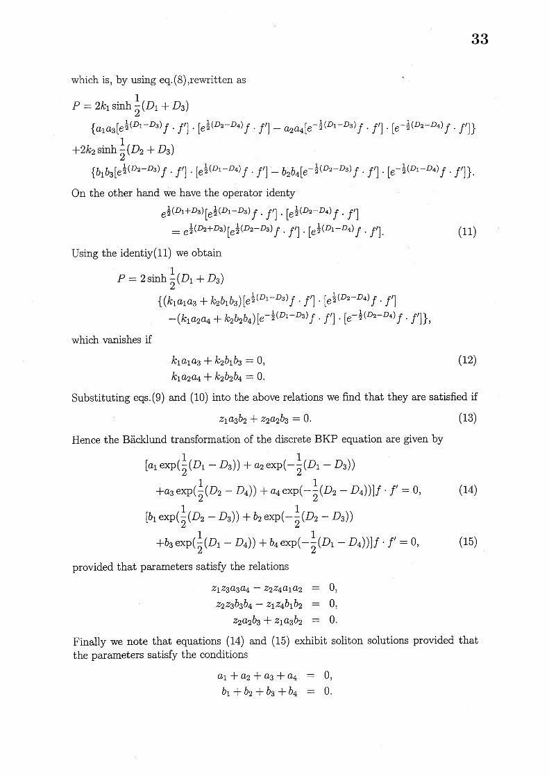
which is, by using $\mathrm{e}\mathrm{q}.(8),\mathrm{r}\mathrm{e}\mathrm{w}\mathrm{r}\mathrm{i}\mathrm{t}\mathrm{t}\mathrm{e}\mathrm{n}$ as
$P=2k_{1} \sinh\frac{1}{2}(D_{1}+D_{3})$
$\{a_{1}a_{3}[e^{\frac{1}{2}}-3)f(D1D. f;]\cdot[e\frac{1}{2}(D2-D_{4})f\cdot f’]-a_{2}a_{4}[e-\frac{1}{2}(D_{1}-D_{3})f\cdot f’]\cdot[e-\frac{1}{2}(D_{2}-D_{4})f\cdot f’]\}$
$+2k_{2} \sinh\frac{1}{2}(D_{2}+D_{3})$
$\{b_{1}b_{3}[e\frac{1}{2}(D_{2}-D_{3})f\cdot f’]\cdot[e\frac{1}{2}(D1-D_{4})f\cdot f’]-b2b_{4}[e-\frac{1}{2}(D2-D3)f\cdot f’]\cdot[e^{-(}\frac{1}{2}D_{1}-D_{4})f\cdot f/]\}$ .
On the other hand we have the operator identy$e^{\frac{1}{2}()}D_{1}+D3[e \frac{1}{2}(D1-D_{3})f\cdot f^{J}]\cdot[e^{\frac{1}{2}(-D_{4}}fD_{2}). f^{J}]$
$=e^{\frac{1}{2}()}[D_{2}+D_{3}-D_{3})e^{\frac{1}{2}(D_{2}}f . f’]$ . $[e^{\frac{1}{2}(D_{1}-D_{4}})f . f’]$ . (11)
Using the identiy(ll) we obtain
$P=2 \sinh\frac{1}{2}(D_{1}+D_{3})$
$\{(k_{1}a_{1}a_{3}+k_{2}b_{1}b_{3})[e^{\frac{\mathrm{i}}{2}(D-D_{3}}f1). f’]\cdot[e^{\frac{1}{2}(D_{2}-D_{4}}f)f’]$
$-(k_{1}a_{2}a_{4}+k_{2}b_{2}b_{4})[e- \frac{1}{2}(D1-D_{3})f\cdot f’]\cdot[e^{-\frac{1}{2}()}-D4fD_{2}f’]\}$ ,
which vanishes if
$k_{1}a_{1}a_{3}+k_{2}b_{1}b_{3}=0$ , (12)$k_{1}a_{2}a_{4}+k_{2}b_{2}b_{4}=0$.
Substituting $\mathrm{e}\mathrm{q}_{\mathrm{S}}.(9)$ and (10) into the above relations we find that they are satisfied if
$z_{1}a_{3}b_{2}+z_{2}a_{2}b_{3}=0$ . (13)
Hence the B\"acklund transformation of the discrete BKP equation are given by
$[a_{1} \exp(\frac{1}{2}(D_{1^{-D_{3}))}}+a_{2}\exp(-\frac{1}{2}(D_{1^{-D_{3}))}}$
$+a_{3} \exp(\frac{1}{2}(D_{2^{-D_{4}))}}+a_{4}\exp(-\frac{1}{2}(D_{2^{-}}D_{4}))]f\cdot fJ=0,$ (14)
$[b_{1} \exp(\frac{1}{2}(D2-D_{3}))+b_{2}\exp(-\frac{1}{2}(D_{2}-D_{3}))$
$+b_{3} \exp(\frac{1}{2}(D_{1^{-D_{4}))}}+b_{4}\exp(-\frac{1}{2}(D_{1^{-}}D_{4}))]f\cdot fJ=0,$ (15)
provided that parameters satisfy the relations
$z_{1}z_{3}a_{3}a4-z2Z4a1a2$ $=$ $0$ ,$z_{2}z_{334^{-Z_{1}}}bbz_{4}b_{1}b2$ $=$ $0$ ,
$z_{2}a_{2}b_{3}+z1a_{\mathrm{s}}b_{2}$ $=$ $0$ .
Finally we note that equations (14) and (15) exhibit soliton solutions provided thatthe parameters $\mathrm{s}\mathrm{a}\mathrm{t}\mathrm{i}\mathrm{s}\Phi$ the conditions
$a_{1}+a_{2}+a_{3}+a_{4}$ $=$ $0$ ,$b_{1}+b_{2}+b_{3}+b4$ $=$ $0$ .
33

References[1] Y.Ohta, R.Hirota, S.Tujimoto and T.Imai, ((Casorati and Discrete Gram Type De-
terminant Representations of Solutions to the Discrete KP Hierarchy in BilinearForm”, J.Phy.Soc.Jpn. 62 (1993) 1872.
[2] T. Miwa, Proc.Jpn.Acad. $58\mathrm{A}(1\mathit{9}82)$ 9.
[3] Satoshi Tsujimoto and Ryogo Hirota, $‘(\mathrm{P}\mathrm{f}\mathrm{a}\mathrm{f}\mathrm{f}\mathrm{i}\mathrm{a}\mathrm{n}$ Representation of Solutions to theDiscrete BKP Hierarchy in Bilinear Form”, J.Phy.Soc.Jpn. 65 (1996) 2797.
[4] Masataka Iwao and Ryogo Hirota,(( $\mathrm{S}_{0}1\mathrm{i}\mathrm{t}\mathrm{o}\mathrm{n}$ Solution of a Coupled Modified KdVEquation,J.Phy.Soc.Jpn. 66 (1997) 577.
[5] Masataka Iwao and Ryogo Hirota, “Soliton Solution of a Coupled Derivative Mod-ified KdV Equation, to appear in J.Phy.Soc.Jpn.
34
Top Related