


![Inertial Odometry on Handheld Smartphones · Inertial odometry is concerned with estimation of the change of position over time. The extensive survey of Harle [17] covers many approaches](https://static.fdocuments.in/doc/165x107/5e20397c5606a777765a5caa/inertial-odometry-on-handheld-smartphones-inertial-odometry-is-concerned-with-estimation.jpg)
Languages
Pages
Legal


Event-based Visual Inertial Odometry
Alex Zihao Zhu, Nikolay Atanasov, Kostas Daniilidis
University of Pennsyvlania
alexzhu, atanasov, [email protected]
Abstract
Event-based cameras provide a new visual sensing
model by detecting changes in image intensity asyn-
chronously across all pixels on the camera. By providing
these events at extremely high rates (up to 1MHz), they al-
low for sensing in both high speed and high dynamic range
situations where traditional cameras may fail. In this pa-
per, we present the first algorithm to fuse a purely event-
based tracking algorithm with an inertial measurement unit,
to provide accurate metric tracking of a camera’s full 6dof
pose. Our algorithm is asynchronous, and provides mea-
surement updates at a rate proportional to the camera ve-
locity. The algorithm selects features in the image plane,
and tracks spatiotemporal windows around these features
within the event stream. An Extended Kalman Filter with
a structureless measurement model then fuses the feature
tracks with the output of the IMU. The camera poses from
the filter are then used to initialize the next step of the
tracker and reject failed tracks. We show that our method
successfully tracks camera motion on the Event-Camera
Dataset [16] in a number of challenging situations.
1. Introduction
Event-based cameras capture changes in the scene at ul-
tra high rates (1MHz), and thus enable processing of very
fast motions without suffering from image blur, temporal
aliasing, high bandwidths, or high intensity ranges. Since
no absolute intensity is captured, there is no notion of a
frame that can be read out from the sensor. Hence, none
of the traditional computer vision low- and mid-level tech-
niques like spatial differentiation and spatial segmentation
can be directly applied. While recent approaches [11] tried
to reconstruct frames, we believe that basic geometric es-
timation problems such as visual odometry can be solved
using only features defined by asynchronous events.
In this paper, we introduce a novel feature tracking
method and a visual-inertial odometry estimation scheme
in order to track 6dof pose from events and inertial mea-
surements without using any intensity frames. State of the
art in visual-inertial odometry relies on feature-tracks over
temporal windows [14]. Such tracks are difficult to obtain
among asynchronous events due to the lack of any inten-
sity neighborhood. We propose a data association scheme
where multiple spatially neighboring events are softly as-
sociated with one feature whose motion is computed using
the weighted event positions. This leads to an Expectation-
Maximization algorithm that estimates the optical flow.
Events corrected to the estimated optical flow value are then
used to compute an affine estimate of optical flow with re-
spect to the onset time of the feature. Finally, filter esti-
mates of the 3D rotation are used in a 2-feature RANSAC
inlier selection with the translation direction as unknown.
At no point during feature tracking do we use a fixed tem-
poral window: the spatiotemporal neighborhood is always
defined using the length of the computed optical flow.
Given several feature tracks over time, we employ an Ex-
tended Kalman Filter which estimates all camera poses dur-
ing the lifespan of the features. Similar to the MSCKF [14],
we eliminate the depth from the measurement equations so
that we do not have to keep triangulated features in the state
vector. Our contributions can be summarized as follows:
• A novel event association scheme resulting in robust
feature tracks by employing two EM-steps and vari-
able temporal frames depending on flow and rotation
estimates obtained from the odometry filter.
• The first visual odometry system for event-based cam-
eras that makes use of inertial information.
• We demonstrate results on very fast benchmark se-
quences and we show superiority with respect to clas-
sic temporally sparse KLT features in high speed and
high dynamic range situations.
2. Related Work
Weikersdorfer et al. [22] present the first work on event-
based pose estimation, using a particle filter based on a
known 2D map. They later extend this work in [23] by fus-
ing the previous work with a 2D mapping thread to perform
SLAM in an artificially textured environment. Similarly,
Censi et al. [3] use a known map of active markers to lo-
calize using a particle filter. The work in [7] also assumes a
known set of images, poses and depth maps to perform 6dof
pose estimation using an EKF. Several methods also com-
15391

bine an event-based camera with other sensors to perform
tracking. The work in [2] combines an event-based cam-
era with a separate CMOS camera to estimate inter-frame
motions of the CMOS camera using the events in order to
estimate camera velocity. Similarly, Tedaldi et al. [19] use
the image frames from a DAVIS camera to perform feature
detection and generate a template to track features in the
event stream, which Kueng et al. [12] wrap in a standard
visual odometry framework to perform up to scale pose es-
timation. In [21] an event-based camera is combined with
a depth sensor for 3D mapping, and uses the particle filter
from [22] for localization. However, fusing an event based
camera with a CMOS or depth camera incurs the same costs
as methods that use either camera, such as motion blur and
limited dynamic range. An alternative approach for event-
based pose tracking relies on jointly estimating the original
intensity based image and pose. Kim et al. [10] pose the
problem in an EKF framework, but the method is limited
to estimating rotation only. The authors in [11] extend this
work and use the method in [1] to jointly estimate the im-
age gradient, 3D scene and 6dof pose. Our method is a 6dof
tracking method that works without any prior knowledge of
the scene. In comparison to the latest work in [12], our
method does not require any image frames, and our track-
ing algorithm treats data associations in a soft manner. By
tracking features solely within the event stream, we are able
to track very fast motions and in high dynamic range situa-
tions, without needing to reconstruct the underlying image
gradient as in [11]. Our method also uses soft data associ-
ations, compared to [12] and [11], who make a hard deci-
sion to associate events with the closest projection of a 3D
landmark, leading to the need for bootstrapping in [12]. By
fusing the tracking with information from an IMU, we are
also able to fully reconstruct the camera pose, including the
scale factor, which vision only techniques are unable to do.
3. Problem Formulation
Consider a sensor package consisting of an inertial mea-
surement unit (IMU) and an event-based camera. Without
loss of generality, assume that the camera and IMU frames
are coincident.1 The state of the sensor package:
s :=[
q bg v ba p]
(1)
consists of its position p ∈ R3, its velocity v ∈ R
3, the ori-
entation of the global frame in the sensor frame represented
by a unit quaternion q ∈ SO(3)2, and the accelerometer and
gyroscope measurement biases, ba and bg , respectively.
At discrete times τ1, τ2, . . ., the IMU provides ac-
celeration and angular velocity measurements I :=
1In practice, extrinsic camera/IMU calibration may be performed off-
line [6]. The IMU and camera frames in the DAVIS-240C are aligned.2The bar emphasizes that this quaternion is the conjugate of the unit
quaternion representing the orientation of the sensor in the global frame.
(ak, ωk, τk). The environment, in which the sensor op-
erates, is modeled as a collection of landmarks L := Lj ∈R
3mj=1.
At discrete times t1, t2, . . ., the event-based camera gen-
erates events E := (xi, ti) which measure the perspective
projection3 of the landmark positions as follows:
π(
[X Y Z]T)
:=1
Z
[
XY
]
h(L, s) := π (R (q) (L− p)) (2)
xi = h(Lα(i), s(ti)) + η(ti), η(ti) ∼ N (0,Σ)
where α : N → 1, . . . ,m is an unknown function rep-
resenting the data association between the events E and the
landmarks L and R(q) is the rotation matrix corresponding
to the rotation generated by quaternion q.
Problem 1 (Event-based Visual Inertial Odometry). Given
inertial measurements I and event measurements E , esti-
mate the sensor state s(t) over time.
4. Overview
The visual tracker uses the sensor state and event infor-
mation to track the projections of sets of landmarks, col-
lectively called features, within the image plane over time,
while the filtering algorithm fuses these visual feature tracks
with the IMU data to update the sensor state. In order to
fully utilize the asynchronous nature of event-based cam-
eras, the temporal window at each step adaptively changes
according to the optical flow. The full outline of our algo-
rithm can be found in Fig. 1 and Alg. 1.
Our tracking algorithm leverages the property that all
events generated by the same landmark lie on a curve in
the spatiotemporal domain and, given the parameters of the
curve, can be propagated along the curve in time to a single
point in space (barring error from noise). In addition, the
gradient along this curve at any point in time represents the
optical flow of the landmark projection, at that time. There-
fore, we can reduce the tracking problem to one of finding
the data association between events and landmark projec-
tions, and estimating the gradient along events generated by
the same point.
To simplify the problem, we make the assumption that
optical flow within small spatiotemporal windows is con-
stant. That is, the curves within these windows become
lines, and estimating the flow is equivalent to estimating the
slope of these lines. To impose this constraint, we dynam-
ically update the size of the temporal window, dt, based
on the time for each projected landmark position to travel
k pixels in the image, estimated using the computed opti-
cal flow. This way, we are assuming constant optical flow
for small displacements, which has been shown to hold
3Without loss of generality, the image measurements are expressed in
normalized pixel coordinates. Intrinsic calibration is needed in practice.
5392

Two Point RANSAC
Update
Prediction
Feature Track Server
Reprojection RANSAC
Completed Feature Tracks
Temporal Window Size
Features
State
Lifetime Estimation
Events
Predicted State
Temporal Window Selector
Sensor Output
IMU
# completed tracks
EM 1 EM 2Flow
# features
F eature Trac king
New Feature Detector
Figure 1: EVIO algorithm overview. Data from the event-based camera and IMU is processed in temporal windows determined by our
algorithm. For each temporal window, the IMU values are used to propagate the state, and features are tracked using two expectation
maximization steps that estimate the optical flow of the features and their alignment with respect to a template. Outlier correspondences
are removed, and the results are stored in a feature track server. As features are lost, their feature tracks are parsed through a second
RANSAC step, and the resulting tracks are used to update the sensor state. The estimated optical flows for all of the features are then used
to determine the size of the next temporal window.
in practice. Given these temporal windows, we compute
feature position information within a discrete set of non-
overlapping time windows [T1, T2], [T2, T3], . . . where
Ti+1 − Ti = dti.
Problem 1a (Event-based Feature Tracking). Given event
measurements E , the camera state si := s(Ti) at time Ti
and a temporal window size dti, estimate the feature pro-
jections F(t) for t ∈ [Ti, Ti+1] in the image plane and the
next temporal window size dti+1.
Given the solution to Problem 1a and a set of readings
from the IMU, our state estimation algorithm in Sec. 6
then employs an Extended Kalman Filter with a structure-
less vision model, as first introduced in [14]. Structured
EKF schemes impose vision constraints on all the features
between each two subsquent camera poses, and as a result
optimize over both the camera poses and the feature posi-
tions. A structureless model, on the other hand, allows us to
impose constraints between all camera poses that observe
each feature, resulting in a state vector containing only the
IMU and camera poses. This drastically reduces the size
of the state vector, and allows for marginalization over long
feature tracks. We pose the state estimation problem as the
sub problem below:
Problem 1b (Visual Inertial Odometry). Given inertial
measurements I at times τk, a camera state si at time
Ti, a temporal window size dti, and feature tracks F(t) for
t ∈ [Ti, Ti+1], estimate the camera state si+1.
5. Event-based Feature Tracking
Given a camera state si and a temporal window
[Ti, Ti+1], the goal of Problem 1a is to track a collection
of features F(t) in the image domain for t ∈ [Ti, Ti+1],
Algorithm 1 EVIO
Input: sensor state si, events E , IMU readings I, window size
dtiTrack features f in the event stream, E , given si (Alg. 2)
Select new features in the image plane (Sec. 5.5)
Calculate the size of the next temporal window dti+1 (Sec. 5.4)
Update the state estimate si+1 given f and I (Alg. 3)
whose positions are initialized using traditional image tech-
niques (Sec. 5.5). Our approach performs two expectation-
maximization (EM) optimizations (Sec. 5.1 and Sec. 5.2)
to align a 3-D spatiotemporal window of events with a prior
2-D template in the image plane.
5.1. Optical Flow Estimation
The motion of a feature f(t) in the image plane can be
described using its optical flow f(t) as follows:
f(t) =f(Ti) +
∫ t
Ti
f(ζ)dζ = f(Ti) + (t− Ti)u(t)
where u(t) := 1t−Ti
∫ t
Ti
f(ζ)dζ is the average flow of f(s)
for s ∈ [Ti, t]. If [Ti, Ti+1] is sufficiently small, we can as-
sume that the average flow u is constant and equal to the av-
erage flows of all landmarks Lj whose projections are close
to f in the image plane. To formalize this observation, we
define a spatiotemporal window around f(Ti) as the collec-
tion of events, that propagate backwards to and landmarks
whose projections at time Ti are close to the vicinity of
f(Ti) :
Wi :=(x, t) ∈ E , L ∈ L | ‖(x− tu)− f(Ti)‖ ≤ ξ,
‖l − f(Ti)‖ ≤ ξ, t ∈ [Ti, Ti+1] (3)
where ξ is the window size in pixels, t := t − Ti, l :=h(L, s), as defined in (2).
5393
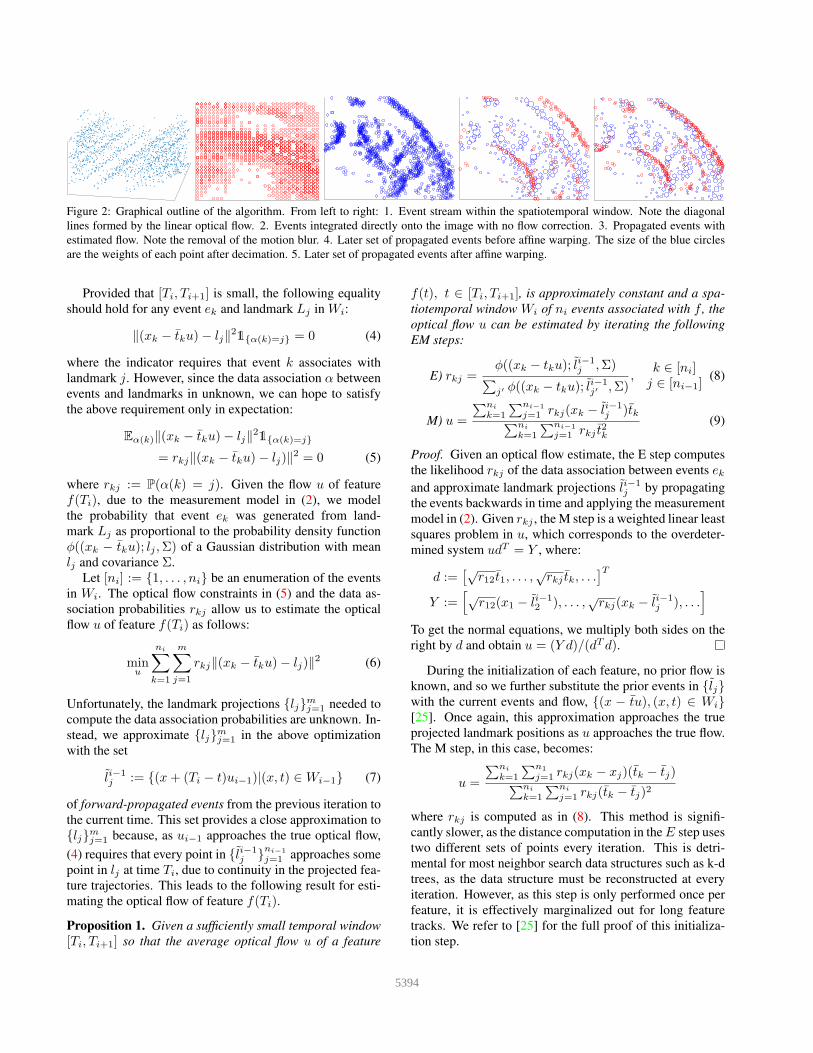
Figure 2: Graphical outline of the algorithm. From left to right: 1. Event stream within the spatiotemporal window. Note the diagonal
lines formed by the linear optical flow. 2. Events integrated directly onto the image with no flow correction. 3. Propagated events with
estimated flow. Note the removal of the motion blur. 4. Later set of propagated events before affine warping. The size of the blue circles
are the weights of each point after decimation. 5. Later set of propagated events after affine warping.
Provided that [Ti, Ti+1] is small, the following equality
should hold for any event ek and landmark Lj in Wi:
‖(xk − tku)− lj‖21α(k)=j = 0 (4)
where the indicator requires that event k associates with
landmark j. However, since the data association α between
events and landmarks in unknown, we can hope to satisfy
the above requirement only in expectation:
Eα(k)‖(xk − tku)− lj‖21α(k)=j
= rkj‖(xk − tku)− lj)‖2 = 0 (5)
where rkj := P(α(k) = j). Given the flow u of feature
f(Ti), due to the measurement model in (2), we model
the probability that event ek was generated from land-
mark Lj as proportional to the probability density function
φ((xk − tku); lj ,Σ) of a Gaussian distribution with mean
lj and covariance Σ.
Let [ni] := 1, . . . , ni be an enumeration of the events
in Wi. The optical flow constraints in (5) and the data as-
sociation probabilities rkj allow us to estimate the optical
flow u of feature f(Ti) as follows:
minu
ni∑
k=1
m∑
j=1
rkj‖(xk − tku)− lj)‖2 (6)
Unfortunately, the landmark projections ljmj=1 needed to
compute the data association probabilities are unknown. In-
stead, we approximate ljmj=1 in the above optimization
with the set
li−1j := (x+ (Ti − t)ui−1)|(x, t) ∈ Wi−1 (7)
of forward-propagated events from the previous iteration to
the current time. This set provides a close approximation to
ljmj=1 because, as ui−1 approaches the true optical flow,
(4) requires that every point in li−1j ni−1
j=1 approaches some
point in lj at time Ti, due to continuity in the projected fea-
ture trajectories. This leads to the following result for esti-
mating the optical flow of feature f(Ti).
Proposition 1. Given a sufficiently small temporal window
[Ti, Ti+1] so that the average optical flow u of a feature
f(t), t ∈ [Ti, Ti+1], is approximately constant and a spa-
tiotemporal window Wi of ni events associated with f , the
optical flow u can be estimated by iterating the following
EM steps:
E) rkj =φ((xk − tku); l
i−1j ,Σ)
∑
j′ φ((xk − tku); li−1j′ ,Σ)
,k ∈ [ni]j ∈ [ni−1]
(8)
M) u =
∑ni
k=1
∑ni−1
j=1 rkj(xk − li−1j )tk
∑ni
k=1
∑ni−1
j=1 rkj t2k(9)
Proof. Given an optical flow estimate, the E step computes
the likelihood rkj of the data association between events ekand approximate landmark projections li−1
j by propagating
the events backwards in time and applying the measurement
model in (2). Given rkj , the M step is a weighted linear least
squares problem in u, which corresponds to the overdeter-
mined system udT = Y , where:
d :=[√
r12t1, . . . ,√rkj tk, . . .
]T
Y :=[√
r12(x1 − li−12 ), . . . ,
√rkj(xk − li−1
j ), . . .]
To get the normal equations, we multiply both sides on the
right by d and obtain u = (Y d)/(dT d).
During the initialization of each feature, no prior flow is
known, and so we further substitute the prior events in ljwith the current events and flow, (x − tu), (x, t) ∈ Wi[25]. Once again, this approximation approaches the true
projected landmark positions as u approaches the true flow.
The M step, in this case, becomes:
u =
∑ni
k=1
∑n1
j=1 rkj(xk − xj)(tk − tj)∑ni
k=1
∑ni
j=1 rkj(tk − tj)2
where rkj is computed as in (8). This method is signifi-
cantly slower, as the distance computation in the E step uses
two different sets of points every iteration. This is detri-
mental for most neighbor search data structures such as k-d
trees, as the data structure must be reconstructed at every
iteration. However, as this step is only performed once per
feature, it is effectively marginalized out for long feature
tracks. We refer to [25] for the full proof of this initializa-
tion step.
5394

5.2. Template Alignment and RANSAC
While Prop. 1 is sufficient to solve Problem 1a, the
feature position estimates may drift as a feature is being
tracked over time, due to noise in each flow estimate. To
correct this drift, we estimate it as the affine warping that
warps likni
k=1 (7) to the template li∗j ni∗
j=1 in the first cam-
era pose that observed the feature. We assume that the cor-
responding landmarks l are planar in 3-D, so that we can
alternatively represent the affine wrapping as a 3-D rotation
and scaling. The 3-D rotation i∗Ri from the current cam-
era pose at Ti to the first camera pose at Ti∗ can be obtained
from the filter used to solve Problem 1b (see Sec. 6). Hence,
in this section we focus on estimating only a scaling σ and
translation b between lik and li∗j . First, we rotate each
point lik to the first camera frame and center at the rotated
feature position as follows:
yik = π
(
i∗Ri
(
lik1
))
− π
(
i∗Ri
(
f(Ti) + uidti1
))
where π is the projection function defined in (2). Note
that lik propagates events to time Ti+1, and so we substi-
tute f(Ti) + uidti as an estimate for f(Ti+1). Then, using
the same idea as in Sec. 5.1, we seek the scaling σ and trans-
lation b that minimize the mismatch between yikni
k=1 and
li∗j ni∗j=1:
minσ,b
ni∑
k=1
ni∗∑
j=1
rkj‖σyik − b− li∗j |2 (10)
This optimization problem has a similar form to problem (6)
and, as before, can be solved via the following EM steps:
E) rkj =φ(yk; l
i∗j ,Σ)
∑
j′ φ(yk; li∗j′ ,Σ)
, k ∈ [ni], j ∈ [ni∗]
M)
y :=1
ni
ni∑
k=1
yk¯l :=
1
ni∗
ni∗∑
j=1
lj
σ =
√
√
√
√
∑ni
k=1
∑ni∗
j=1 rkj(yk − y)T (lj − ¯l)
∑ni
k=1
∑ni∗
j=1 rkj(yk − y)T (yk − y)
b =σ
ni
ni∑
k=1
ni∗∑
j=1
rkjyk − 1
ni∗
ni∑
k=1
ni∗∑
j=1
rkj lj
=σ
ni
ni∑
k=1
yk − 1
ni∗
ni∑
k=1
ni∗∑
j=1
rkj lj
as
ni∗∑
j=1
rkj = 1
(11)
where the M step is solved as in scaled ICP [26].
Algorithm 2 Event-based Feature Tracking
Input
sensor state si, current time Ti, window size dti,events E for t ∈ [Ti, Ti + dti],features f and associated templates li−1, li∗
Tracking
for each feature f do
Find events within Wi (3)
cost←∞while cost > ǫ1 do
Update rkj (8), u (9) and cost (6)
Back-propagate events to Ti using ucost←∞while cost > ǫ2 do
Update rkj (11), (σ, b) (11) and cost (10)
f ← f − b+ dtiu
dti+1 ← 3/median(‖u‖) (Sec. 5.4)
return f and dti+1
5.3. Outlier Rejection
In order to remove outliers from the above optimizations,
only pairs of points ((xk− tku) and (σyk−b)), and approx-
imate projected landmarks, lj , with Mahalanobis distance4
below a set threshold are used in the optimizations. This
also serves the purpose of heavily reducing the number of
computation.
After all of the features have been updated, two-point
RANSAC [20] is performed given the feature correspon-
dences and the rotation between the frames from the state
to remove features whose tracking have failed. Given two
correspondences and the rotation, we estimate the essential
matrix, and evaluate the Sampson error5 on the set of corre-
spondences to determine the inlier set.
The complete feature tracking procedure is illustrated in
Fig. 2 and summarized in Alg. 2.
5.4. Temporal Window Size Selection
To set the temporal window size such that each feature
moves k pixels within the window, we leverage the con-
cept of ‘event lifetimes’ [15]. Given an estimate of the
optical flow, u, of a feature f at a given time, Ti, the ex-
pected time for the feature to move 1 pixel in the image
is 1‖u‖2
. Therefore, to estimate the time for a feature to
move k pixels, the time is simply dt(f) = k‖u‖2
Given a set
of tracked features, we set the next temporal window size
as: dti+1 = median(dt(f) | f ∈ F). Assuming that
4The Mahalanobis distance between a point x and a distribu-
tion with mean µ and standard distribution Σ is defined as: d :=√
(x− µ)TΣ(x− µ).5Given a correspondence between two points x1, x2 and the cam-
era translation t and rotation R between the points, the Essential ma-
trix is defined as: E = t × R, and the sampson error is defined as:
e =xT
2Ex1
(Ex1)2
1+(Ex1)
2
2+(Ex2)
2
1+(Ex2)
2
2
5395

the differences in depth between the features is not large,
this window size should ensure that each feature will travel
roughly k pixels in the next temporal window. For all of our
experiments, k is set to 3.
5.5. Feature Detection
Like traditional image based tracking techniques, our
event-based feature tracker suffers from the aperture prob-
lem. Given a feature window with only a straight line, we
can only estimate the component of the optical flow that is
normal to the slope of this line. As a result, features must
be carefully selected to avoid selecting windows with a sin-
gle strong edge direction. To do so, we find ’corners’ in the
image that have strong edges in multiple directions. In or-
der to produce an image from the event stream, we simply
take the orthogonal projection of the events onto the image
plane. As we constrain each temporal window such that fea-
tures only travel k pixels, this projection should reconstruct
the edge map of the underlying image, with up to k pixels
of motion blur, which should not be enough to corrupt the
corner detection. The actual corner detection is performed
with FAST corners [17], with the image split into cells of
fixed size, and the corner with the highest Shi-Tomasi score
[18] within each cell being selected, as in [5].
6. State Estimation
To estimate the 3D pose of the camera over time, we em-
ploy an Extended Kalman Filter with a structureless vision
model, as first developed in [14]. For compactness, we do
not expand on the fine details of the filter, and instead re-
fer interested readers to [13] and [14]. At time Ti, the filter
tracks the current sensor state (1) as well as all past camera
poses that observed a feature that is currently being tracked.
The full state, then, is:
Si := S(Ti) =[
sTi q(Ti−n)T p(Ti−n)
T . . . q(Ti)T p(Ti)
T]T
where n is the length of the oldest tracked feature.
Between update steps, the prediction for the sensor state
is propagated using the IMU measurements that fall in be-
tween the update steps. Note that, due to the high temporal
resolution of the event based camera, there may be mul-
tiple update steps in between each IMU measurement. In
that case, we use the last IMU measurement to perform the
propagation.
Given linear acceleration ak and angular velocity ωk
measurements, the sensor state is propagated using 5th or-
der Runge-Kutta integration:
˙q(τk) =1
2Ω(ωk − bg(τk))q(τk)
p(τk) = v(τk)
v(τk) = R(q(τk))T (ak − ba(τk)) + g
ba(τk) = 0
bg(τk) = 0(12)
Algorithm 3 State Estimation
Input
sensor state si, features fIMU values I for t ∈ [Ti, Ti + dti]
Filter
Propagate the sensor state mean and covariance (12)
Augment a new camera state
for each filter track to be marginalized do
Remove inconsistent observations
Triangulate the feature using GN Optimization
Compute the uncorrelated residuals r(j)0 (13)
Stack all of the r(j)0
Perform QR decomposition to get the final residual (14)
Update the state and state covariance
To perform the covariance propagation, we adopt the dis-
crete time model and covariance prediction update pre-
sented in [9].
When an update from the tracker arrives, we augment the
state with a new camera pose at the current time, and update
the covariance using the Jacobian that maps the IMU state
to the camera state.
We then process any discarded features that need to be
marginalized. For any such feature fj , the 3D position of
the feature Fj can be estimated using its past observations
and camera poses by Gauss Newton optimization, assuming
the camera poses are known [4]. The projection of this esti-
mate into a given camera pose can then be computed using
(2). The residual, r(j), for each feature at each camera pose
is the difference between the observed and estimated feature
positions. We then left multiply r(j) by the left null space,
A, of the feature Jacobian, HF , as in [14], to eliminate the
feature position up to a first order approximation:
r(j)0 =AT r(j)
≈ATH(j)S S +ATH
(j)F Fj +ATn(j) := H
(j)0 S + n
(j)0
(13)
rn =QT1 r0 (14)
H0 =[
Q1 Q2
]
[
TH
0
]
The elimination procedure is performed for all features, and
the remaining uncorrelated residuals, r(j)0 are stacked to ob-
tain the final residual r0. As in [14], we perform one final
step to reduce the dimensionality of the above residual. Tak-
ing the QR decomposition of the matrix H0, we can elimi-
nate a large part of the residual (14). The EKF update step
is then ∆S = Krn, where K is the Kalman gain.
When a feature track is to be marginalized, we apply a
second RANSAC step to find the largest set of inliers that
project to the same point in space, based on reprojection
error. This removes moving objects and other erroneous
measurements from the track.
5396

Figure 3: Example images with overlaid events from each sequence. From left to right: shapes, poster, boxes, dynamic, HDR.
0 10 20 30 40 50 60
Time (s)
0
0.05
0.1
0.15
0.2
0.25
Te
mp
ora
l w
ind
ow
siz
e (
s)
0 5 10 15 20 25 30
Distance traveled (m)
0
0.05
0.1
0.15
0.2
0.25
0.3
0.35
0.4
Err
or
dynamic_translation Raw Error
Pos Err (m)
Rot Err (rad)
0 10 20 30 40 50 60
Distance traveled (m)
0
0.2
0.4
0.6
0.8
1
1.2
1.4
Err
or
hdr_boxes Raw Error
Pos Err (m)
Rot Err (rad)
Figure 4: Left to right: Temporal window sizes in the hdr boxes sequence, absolute position and rotation errors for the dynamic translation
and hdr boxes sequences. EVIO results are solid, while KLT results are dashed.
1.2-1.8
1.25
1.3
2.2
1.35
1.4
z (
m)
1.45
1.5
-1.6
1.55
2
y (m)x (m)
-1.41.8 -1.2
-11.6
EVIO
OptiTrack
0.8
0.9
1
1.1
1
1.2
1.3
1.4
z (
m)
1.5
1.6
0.60.5 0.8
x (m) y (m)
101.2
-0.5 1.4
EVIO
OptiTrack
Figure 5: Sample tracked trajectories from shapes translation (top)
and hdr boxes (bottom). The first 15 seconds of each sequence are
shown, to avoid clutter as the trajectories tends to overlap.
7. Experiments
We evaluate the accuracy of our filter on the Event-
Camera Dataset [16]. The Event-Camera Dataset contains
many sequences captured with a DAVIS-240C camera with
information from the events, IMU and images. A number
of sequences were also captured in an indoor OptiTrack en-
vironment, which provides 3D groundtruth pose.
Throughout all experiments, dt0 is initialized as the time
to collect 50000 events. The covariance matrices for the
two EM steps are set as 2I , where I is the identity matrix.
In each EM step, the template point sets lj are subsam-
pled using sphere decimation [8], with radius 1 pixel. As
EVIO KLTVIO
Sequence Mean
Position
Error
(%)
Mean
Rotation
Error
(deg/m)
Mean
Position
Error
(%)
Mean
Rotation
Error
(deg/m)
shapes translation 2.42 0.52 1.98 0.04
shapes 6dof 2.69 0.40 8.95 0.06
poster translation 0.94 0.02 0.97 0.01
poster 6dof 3.56 0.56 2.17 0.08
hdr poster 2.63 0.11 2.67 0.09
boxes translation 2.69 0.09 2.28 0.01
boxes 6dof 3.61 0.34 2.91 0.03
hdr boxes 1.23 0.05 5.65 0.11
dynamic translation 1.90 0.02 2.12 0.03
dynamic 6dof 4.07 0.56 4.49 0.05
Table 1: Comparison of average position and rotation error statis-
tics between EVIO and KLTVIO across all sequences. Position
errors are reported as a percentage of distance traveled. Rotation
errors are reported in degrees over distance traveled.
both sets of templates remain constant in both EM steps,
we are able to generate a k-d tree structure to perform the
Mahalanobis distance checks and E-Steps, generating a sig-
nificant boost in speed. The Mahalanobis threshold was set
at 4 pixels.
At present, our implementation of the feature tracker in
C++ is able to run in real time for up to 15 features for
moderate optical flows on a 6 core Intel i7 processor. The
use of a prior template for flow estimation, and 3D rota-
tion for template alignment has allowed for very significant
improvements in runtime, as compared to [25]. In these ex-
periments, 100 features with spatial windows of 31x31 are
tracked. Unfortunately, as we must process a continuous set
of time windows, there is no equivalent of lower frame rates,
so tracking a larger number of features results in slower than
realtime performance as of now. However, we believe, with
further optimization, that this algorithm can run in real time.
5397

For our evaluation, we examine only sequences with
ground truth and IMU (examples in Fig. 3), omitting the
outdoor and simulation sequences. In addition, we omit the
rotation only sequences, as translational motion is required
to triangulate points between camera poses.
We compare our event based tracking algorithm with
a traditional image based algorithm by running the KLT
tracker on the images from the DAVIS camera, and pass-
ing the tracked features through the same EKF pipeline (we
will call this KLTVIO). The MATLAB implementation of
KLT is used.
In Fig. 4, we show the temporal size at each iteration.
Note that the iterations near the end of the sequence are
occurring at roughly 100Hz.
For quantitative evaluation, we compare the position and
rotation estimates from both EVIO and KLTVIO against
the ground truth provided. Given a camera pose estimate
at time Ti, we linearly interpolate the pose of the two
nearest OptiTrack measurements to estimate the ground
truth pose at this time. Position errors are computed us-
ing Euclidean distance, and rotation errors are computed as
errrot =12 tr(I3−RT
EV IOROptiTrack). Sample results for
the dynamic translation and hdr boxes sequences are shown
in Fig. 4.
In Fig. 5, we also show two sample trajectories tracked
by our algorithm over a 15 second period, where we can
qualitatively see that the estimated trajectory is very similar
to the ground truth.
In Table 1, we present the mean position error as a per-
centage of total distance traveled and rotation error over dis-
tance traveled for each sequence, which are common met-
rics for VIO applications [8].
8. Discussion
From the results, we can see that our method performs
comparably to the image based method in the normal se-
quences. In particular, EVIO outperforms KLTVIO in se-
quences where event-based cameras have an advantage,
such as with high speed motions in the dynamic sequences
and the high dynamic range scenes. On examination of
the trajectories (please see the supplemental video), our
method is able to reconstruct the overall shape, albeit with
some drift, while the KLT based method is prone to errors
where the tracking completely fails. Unfortunately, as the
workspace for the sequences is relatively small (3m x 3m),
it is difficult to distinguish between drift and failure from
error values alone.
In Table 1, we can see that our rotation errors are typ-
ically much larger than expected. On inspection of the
feature tracks (please see the supplemental video), we can
see that, while the majority of the feature tracks are very
good, and most failed tracks are rejected by the RANSAC
steps, there are still a small, but significant portion of fea-
ture tracks that fail, but are not immediately rejected by
Figure 6: Challenging situations with events within a temporal
window (red) overlaid on top of the intensity image. From left to
right: boxes 6dof sequence: majority back wall with no events.
shapes 6dof: events only generate on edges of a sparse set of
shapes, with portions also mostly over a textureless wall
RANSAC. This equates to the feature tracker estimating
the correct direction of the feature’s motion (i.e. along the
epipolar line), but with an incorrect magnitude. Unfortu-
nately, this is an error that two-point RANSAC cannot re-
solve. In addition, the error in EM2 can also fail to detect
a failed track, for example in situations where the template
points are very dense, and so every propagated event is close
to a template point, regardless of the scaling and translation.
As the EKF is a least squares minimizer, the introduction of
any such outlier tracks has a significant effect on the state
estimate. However, overall, our event based feature tracking
is typically able to track more features over longer periods
of time than the image based technique, and we believe that
we should be able to remove these outliers and significantly
reduce the errors by applying more constraints to the feature
motion in future works. These outliers are less common in
KLTVIO, as it has been tuned to be over conservative when
rejecting feature motions (although this results in shorter
feature tracks, overall).
In addition, one of the main challenging aspects of this
dataset stems from the fact that, as event-based cameras
tend to only trigger events over edge-like features, low tex-
ture areas generate very few events, if any. In many of the
sequences, the camera passes over textureless areas, such as
the back wall of the room, resulting in no events generating
in the parts of the image containing the wall. As a result,
no features are tracked over these areas. When these areas
in the image are large, as in the examples in Figure 6, this
introduces biases into the filter pose estimate, and increases
tracking error. This typically tends to affect EVIO more
than KLTVIO, as areas where no events generate may still
have some texture, with the exception being the shapes 6dof
sequence, where the KLT tracker fails at the beginning. As
a result, this lack of information is a significant contributor
to feature track failure.
In conclusion, we have presented a novel event-based
visual inertial odometry algorithm that uses event based
feature tracking with probabilistic data associations and an
EKF with a structureless vision model. We show that our
work is comparable to vision based tracking algorithms, and
that it is capable of tracking long camera trajectories with a
small amount of drift.
5398

References
[1] P. Bardow, A. J. Davison, and S. Leutenegger. Simultaneous
optical flow and intensity estimation from an event camera.
In Proceedings of the IEEE Conference on Computer Vision
and Pattern Recognition, pages 884–892, 2016. 2
[2] A. Censi and D. Scaramuzza. Low-latency event-based vi-
sual odometry. In 2014 IEEE International Conference on
Robotics and Automation (ICRA), pages 703–710. IEEE,
2014. 2
[3] A. Censi, J. Strubel, C. Brandli, T. Delbruck, and D. Scara-
muzza. Low-latency localization by active led markers track-
ing using a dynamic vision sensor. In 2013 IEEE/RSJ In-
ternational Conference on Intelligent Robots and Systems,
pages 891–898. IEEE, 2013. 1
[4] L. Clement, V. Peretroukhin, J. Lambert, and J. Kelly. The
battle for filter supremacy: A comparative study of the multi-
state constraint kalman filter and the sliding window filter.
In Computer and Robot Vision (CRV), 2015 12th Conference
on, pages 23–30, 2015. 6
[5] C. Forster, M. Pizzoli, and D. Scaramuzza. Svo: Fast semi-
direct monocular visual odometry. In Robotics and Automa-
tion (ICRA), 2014 IEEE International Conference on, pages
15–22. IEEE, 2014. 6
[6] P. Furgale, J. Rehder, and R. Siegwart. Unified temporal and
spatial calibration for multi-sensor systems. In IEEE/RSJ
Int. Conf. on Intelligent Robots and Systems (IROS), pages
1280–1286, 2013. 2
[7] G. Gallego, J. E. Lund, E. Mueggler, H. Rebecq, T. Delbruck,
and D. Scaramuzza. Event-based, 6-dof camera tracking for
high-speed applications. arXiv preprint arXiv:1607.03468,
2016. 1
[8] A. Geiger, P. Lenz, and R. Urtasun. Are we ready for au-
tonomous driving? the kitti vision benchmark suite. In
Conference on Computer Vision and Pattern Recognition
(CVPR), 2012. 7, 8
[9] J. A. Hesch, D. G. Kottas, S. L. Bowman, and S. I. Roumeli-
otis. Observability-constrained vision-aided inertial naviga-
tion. University of Minnesota, Dept. of Comp. Sci. & Eng.,
MARS Lab, Tech. Rep, 1, 2012. 6
[10] H. Kim, A. Handa, R. Benosman, S.-H. Ieng, and A. J. Davi-
son. Simultaneous mosaicing and tracking with an event
camera. In British Machine Vision Conference. IEEE, 2014.
2
[11] H. Kim, S. Leutenegger, and A. J. Davison. Real-time 3d
reconstruction and 6-dof tracking with an event camera. In
European Conference on Computer Vision, pages 349–364.
Springer, 2016. 1, 2
[12] B. Kueng, E. Mueggler, G. Gallego, and D. Scaramuzza.
Low-latency visual odometry using event-based feature
tracks. In IEEE/RSJ International Conference on Intelligent
Robots and Systems (IROS), number EPFL-CONF-220001,
2016. 2
[13] A. I. Mourikis and S. I. Roumeliotis. A multi-state constraint
kalman filter for vision-aided inertial navigation. 2006. 6
[14] A. I. Mourikis and S. I. Roumeliotis. A multi-state constraint
kalman filter for vision-aided inertial navigation. Technical
report, 2007. 1, 3, 6
[15] E. Mueggler, C. Forster, N. Baumli, G. Gallego, and
D. Scaramuzza. Lifetime estimation of events from dynamic
vision sensors. In 2015 IEEE International Conference on
Robotics and Automation (ICRA), pages 4874–4881. IEEE,
2015. 5
[16] E. Mueggler, H. Rebecq, G. Gallego, T. Delbruck, and
D. Scaramuzza. The event-camera dataset and simulator:
Event-based data for pose estimation, visual odometry, and
slam. 1, 7
[17] E. Rosten, R. Porter, and T. Drummond. Faster and bet-
ter: A machine learning approach to corner detection. IEEE
transactions on pattern analysis and machine intelligence,
32(1):105–119, 2010. 6
[18] J. Shi et al. Good features to track. In Computer Vi-
sion and Pattern Recognition, 1994. Proceedings CVPR’94.,
1994 IEEE Computer Society Conference on, pages 593–
600. IEEE, 1994. 6
[19] D. Tedaldi, G. Gallego, E. Mueggler, and D. Scaramuzza.
Feature detection and tracking with the dynamic and active-
pixel vision sensor (davis). In Event-based Control, Com-
munication, and Signal Processing (EBCCSP), 2016 Second
International Conference on, pages 1–7. IEEE, 2016. 2
[20] C. Troiani, A. Martinelli, C. Laugier, and D. Scaramuzza.
2-point-based outlier rejection for camera-imu systems with
applications to micro aerial vehicles. In 2014 IEEE Inter-
national Conference on Robotics and Automation (ICRA),
pages 5530–5536. IEEE, 2014. 5
[21] D. Weikersdorfer, D. B. Adrian, D. Cremers, and J. Conradt.
Event-based 3d slam with a depth-augmented dynamic vi-
sion sensor. In IEEE Int. Conf. on Robotics and Automation
(ICRA), pages 359–364, 2014. 2
[22] D. Weikersdorfer and J. Conradt. Event-based particle fil-
tering for robot self-localization. In Robotics and Biomimet-
ics (ROBIO), 2012 IEEE International Conference on, pages
866–870. IEEE, 2012. 1, 2
[23] D. Weikersdorfer, R. Hoffmann, and J. Conradt. Simulta-
neous localization and mapping for event-based vision sys-
tems. In International Conference on Computer Vision Sys-
tems, pages 133–142. Springer Berlin Heidelberg, 2013. 1
[24] A. Zhu, N. Atanasov, and K. Daniilidis. Event-based feature
tracking with probabilistic data association. 2016.
[25] A. Z. Zhu, N. Atanasov, and K. Daniilidis. Event-based fea-
ture tracking with probabilistic data association. In 2017
IEEE International Conference on Robotics and Automation
(ICRA). IEEE, 2017. 4, 7
[26] T. Zinßer, J. Schmidt, and H. Niemann. Point set registra-
tion with integrated scale estimation. In Eighth International
Conference on Pattern Recognition and Image Processing,
volume 116, page 119, 2005. 5
5399
Top Related