


Languages
Pages
Legal

Evaluate, Modify, and Adapt the ConcreteWorks Software for Iowa’s UseFinal ReportMarch 2020
Sponsored byIowa Highway Research Board(IHRB Project TR-712)Iowa Department of Transportation(InTrans Project 16-581)
About the Institute for TransportationThe mission of the Institute for Transportation (InTrans) at Iowa State University is to develop and implement innovative methods, materials, and technologies for improving transportation efficiency, safety, reliability, and sustainability while improving the learning environment of students, faculty, and staff in transportation-related fields.
Iowa State University Nondiscrimination Statement Iowa State University does not discriminate on the basis of race, color, age, ethnicity, religion, national origin, pregnancy, sexual orientation, gender identity, genetic information, sex, marital status, disability, or status as a US veteran. Inquiries regarding nondiscrimination policies may be directed to the Office of Equal Opportunity, 3410 Beardshear Hall, 515 Morrill Road, Ames, Iowa 50011, telephone: 515-294-7612, hotline: 515-294-1222, email: [email protected].
Disclaimer NoticeThe contents of this report reflect the views of the authors, who are responsible for the facts and the accuracy of the information presented herein. The opinions, findings and conclusions expressed in this publication are those of the authors and not necessarily those of the sponsors.
The sponsors assume no liability for the contents or use of the information contained in this document. This report does not constitute a standard, specification, or regulation.
The sponsors do not endorse products or manufacturers. Trademarks or manufacturers’ names appear in this report only because they are considered essential to the objective of the document.
Iowa DOT Statements Federal and state laws prohibit employment and/or public accommodation discrimination on the basis of age, color, creed, disability, gender identity, national origin, pregnancy, race, religion, sex, sexual orientation or veteran’s status. If you believe you have been discriminated against, please contact the Iowa Civil Rights Commission at 800-457-4416 or the Iowa Department of Transportation affirmative action officer. If you need accommodations because of a disability to access the Iowa Department of Transportation’s services, contact the agency’s affirmative action officer at 800-262-0003.
The preparation of this report was financed in part through funds provided by the Iowa Department of Transportation through its “Second Revised Agreement for the Management of Research Conducted by Iowa State University for the Iowa Department of Transportation” and its amendments.
The opinions, findings, and conclusions expressed in this publication are those of the authors and not necessarily those of the Iowa Department of Transportation.
Technical Report Documentation Page
1. Report No. 2. Government Accession No. 3. Recipient’s Catalog No.
IHRB Project TR-712
4. Title and Subtitle 5. Report Date
Evaluate, Modify, and Adapt the ConcreteWorks Software for Iowa’s Use March 2020
6. Performing Organization Code
7. Author(s)
Kejin Wang (orcid.org/0000-0002-7466-3451), Yogiraj Sargam
(orcid.org/0000-0001-9980-3038), Kyle Riding (orcid.org/0000-0001-8083-
554X), Mahmoud Faytarouni (orcid.org/0000-0003-4231-158X), Charles
Jahren (orcid.org/0000-0003-2828-8483), and Jay Shen (orcid.org/0000-0002-
8201-5569)
8. Performing Organization Report No.
InTrans Project 16-581
9. Performing Organization Name and Address 10. Work Unit No. (TRAIS)
Institute for Transportation
Iowa State University
2711 South Loop Drive, Suite 4700
Ames, IA 50010-8664
11. Contract or Grant No.
12. Sponsoring Organization Name and Address 13. Type of Report and Period Covered
Iowa Highway Research Board
Iowa Department of Transportation
800 Lincoln Way
Ames, IA 50010
Final Report
14. Sponsoring Agency Code
IHRB Project TR-712
15. Supplementary Notes
Visit https://intrans.iastate.edu/ for color pdfs of this and other research reports.
16. Abstract
The early-age thermal development in mass concrete has a significant impact on the performance and long-term serviceability of
mass concrete structures, such as bridge foundations. Great efforts have been made on predicting and controlling the thermal
development in mass concrete. ConcreteWorks has been increasingly used for this purpose. However, previous research in Iowa
indicated that, although user-friendly, the public ConcreteWorks program has some features that do not fit Iowa concrete well.
The present research aimed at modifying the ConcreteWorks software for Iowa’s use, particularly for the prediction of thermal
behavior of mass concrete elements with a smallest dimension of 6.5 feet or less.
In this study, the input and output parameters of ConcreteWorks that need to be modified for Iowa’s use were identified. The key
properties (heat of hydration, thermal conductivity, mechanical properties, etc.) of typical Iowa concrete mixes required by
ConcreteWorks for thermal predictions were tested. The Iowa environmental data and Iowa Department of Transportation (DOT)
temperature differential limits were incorporated into the modified ConcreteWorks program. An initial soil temperature model
was added. Thermal analyses were conducted on a real-time mass concrete project (the I-35 NB to US 30 WB [Ramp H] bridge)
using both the unmodified and modified ConcreteWorks software as well as 4C-Temp&Stress software, and the predicted
temperature developments were compared with those monitored from the field site.
The results indicate that the modified ConcreteWorks software predicts the early-age temperature profile, maturity, and strength
of Iowa mass concrete quite well. As many default data in the public ConcreteWorks software are replaced with Iowa concrete
values, the modified software is even more user-friendly and reliable for Iowa’s use. A hands-on workshop on learning how to
use ConcreteWorks was welcomed by Iowa engineers. Recommendations are made in this report for effective use of the modified
ConcreteWorks software in Iowa and for further research in this area.
17. Key Words 18. Distribution Statement
4C-Temp&Stress—ConcreteWorks—mass concrete—thermal analysis No restrictions.
19. Security Classification (of this
report)
20. Security Classification (of this
page)
21. No. of Pages 22. Price
Unclassified. Unclassified. 138 NA
Form DOT F 1700.7 (8-72) Reproduction of completed page authorized

EVALUATE, MODIFY, AND ADAPT THE
CONCRETEWORKS SOFTWARE FOR IOWA’S
USE
Final Report
March 2020
Principal Investigator
Kejin Wang, Professor
Institute for Transportation, Iowa State University
Co-Principal Investigators
Kyle Riding, Associate Professor
Department of Civil and Coastal Engineering, Kansas State University
Chuck Jahren, Professor
Civil, Construction, and Environmental Engineering, Iowa State University
Jay Shen, Associate Professor
Civil, Construction, and Environmental Engineering, Iowa State University
Research Assistants
Yogiraj Sargam and Mahmoud Faytarouni
Authors
Kejin Wang, Yogiraj Sargam, Kyle Riding, Mahmoud Faytarouni, Charles Jahren, and Jay Shen
Sponsored by
Iowa Highway Research Board and
Iowa Department of Transportation
(IHRB Project TR-712)
Preparation of this report was financed in part
through funds provided by the Iowa Department of Transportation
through its Research Management Agreement with the
Institute for Transportation
(InTrans Project 16-581)
A report from
Institute for Transportation
Iowa State University
2711 South Loop Drive, Suite 4700
Ames, IA 50010-8664
Phone. 515-294-8103 / Fax. 515-294-0467
https://intrans.iastate.edu/

v
TABLE OF CONTENTS
ACKNOWLEDGMENTS ............................................................................................................. xi
EXECUTIVE SUMMARY ......................................................................................................... xiii
1. INTRODUCTION .......................................................................................................................1
Problem Statement ...............................................................................................................1 Goals and Objectives ...........................................................................................................1 Tasks Conducted ..................................................................................................................2 Scope of Report....................................................................................................................2
2. SOFTWARE REVIEW ...............................................................................................................4
ConcreteWorks Review .......................................................................................................4 4C-Temp&Stress Review ....................................................................................................7
Comparison of Inputs and Prediction Models .....................................................................9
3. EXPERIMENTS AND TEST METHODS ...............................................................................13
Materials and Mixes ...........................................................................................................13
Tests and Methods .............................................................................................................16
4. RESULTS AND DISCUSSION ................................................................................................30
Properties of Fresh Concrete ..............................................................................................30
Properties of Hardened Concrete .......................................................................................30 Semi-Adiabatic Calorimetry ..............................................................................................42
Thermal Conductivity ........................................................................................................44 Coefficient of Thermal Expansion .....................................................................................45
5. FIELD INVESTIGATION ........................................................................................................46
Investigation before Placement of Concrete ......................................................................48
Investigation during Placement of Concrete ......................................................................53 Investigation after Placement of Concrete .........................................................................57
6. CONCRETEWORKS MODIFICATIONS ...............................................................................69
Modifications in Input........................................................................................................69 Modifications in Output .....................................................................................................74
7. THERMAL ANALYSIS USING CONCRETEWORKS AND 4C ..........................................77
Analysis of the Field Mix ..................................................................................................77
Analysis of Laboratory Mixes ...........................................................................................88
8. WORKSHOP AND SOFTWARE DOWNLOAD DETAILS .................................................106
9. CONCLUSIONS AND RECOMMENDATIONS ..................................................................108
REFERENCES ............................................................................................................................111
APPENDIX A. CALIBRATION OF ISOTHERMAL CALORIMETER ..................................113
APPENDIX B. STEPS FOR BUILDING A SEMI-ADIABATIC CALORIMETER ................115

vi
APPENDIX C. CALIBRATION OF SEMI-ADIABATIC CALORIMETER............................119
APPENDIX D. PROCEDURE TO ASSEMBLE THE THERMAL CONDUCTIVITY
TEST SETUP ...................................................................................................................121
APPENDIX E. CALIBRATION OF THERMAL CONDUCTIVITY APPARATUS ...............123
vii
LIST OF FIGURES
Figure 2.1. Temperature prediction model in ConcreteWorks ........................................................5 Figure 2.2. Flowchart of the thermal stress modeling in ConcreteWorks .......................................6
Figure 2.3. Process of performing an analysis in 4C-Temp & Stress program ...............................9 Figure 3.1. Aggregate gradation curves: ASTM C33 (top) and 8/18 gradation (bottom) .............15 Figure 3.2. Isothermal calorimeter (left) and channels for holding samples (right) ......................18 Figure 3.3. Arrhenius plot ..............................................................................................................21 Figure 3.4. Semi-adiabatic calorimeter ..........................................................................................22
Figure 3.5. Thermal conductivity test setup...................................................................................26 Figure 3.6. Coefficient of thermal expansion test equipment ........................................................28 Figure 4.1. Compressive strength development .............................................................................31
Figure 4.2. Compressive strength – TTF best-fit curve .................................................................33 Figure 4.3. Rate of heat generation (Mix 1) ...................................................................................34 Figure 4.4. Cumulative heat (Mix 1) .............................................................................................35
Figure 4.5. Rate of heat and cumulative heat (Mix 2) ...................................................................36 Figure 4.6. Rate of heat and cumulative heat (Mix 3) ...................................................................37 Figure 4.7. Rate of heat and cumulative heat (Mix 4) ...................................................................38
Figure 4.8. Arrhenius plots for activation energy ..........................................................................40 Figure 4.9. Measured semi-adiabatic (top) and calculated adiabatic temperature (bottom) ..........43
Figure 4.10. Temperature development during thermal conductivity test .....................................44 Figure 5.1. Location of the I-35 to US 30 Bridge ..........................................................................46 Figure 5.2. Locations of all six piers..............................................................................................47
Figure 5.3. Dimensions of all six piers ..........................................................................................47
Figure 5.4. Subsurface profile of Pier 4 job site (left), Thickness of layers (top right), and
Excavated soil (bottom right) ........................................................................................48 Figure 5.5. Limestone subbase with steel bearing H-piles (left) and front elevation of
footing with subbase (right) ..........................................................................................49 Figure 5.6. Formwork used in Pier 4 footing .................................................................................50
Figure 5.7. Locations of temperature sensors installed in Pier 4 footing ......................................50 Figure 5.8. Data loggers (left), primary and backup sensors (center), and measurement of
sensor locations (right) ..................................................................................................51
Figure 5.9. Predicted maximum temperature at the core, ambient temperature, and
temperature differential compared to Iowa DOT specified limits ................................53
Figure 5.10. Pouring concrete using pump (left) and compaction using vibrator (right) ..............54 Figure 5.11. Weather station at job site .........................................................................................55
Figure 5.12. Casting cylindrical specimens (left) and curing specimens in field conditions
at the job site (right) ......................................................................................................56 Figure 5.13. Insulation blanket over formwork .............................................................................56 Figure 5.14. Recorded temperature data of all sensors ..................................................................59 Figure 5.15. Differential temperature in concrete footing with age ..............................................59
Figure 5.16. Temperature (top) and relative humidity (bottom) variations with age ....................62 Figure 5.17. Insulation and formwork removal stage: Day 0 Insulation blanket (top left),
Day 5. Formwork removed from three sides (top right), Day 10 Exposed
concrete surface (bottom left), and Day 12 Footing backfilled with soil (bottom
right) ..............................................................................................................................63
viii
Figure 5.18. Compressive strength development (left) and compressive strength-TTF curve
(right).............................................................................................................................65 Figure 5.19. Variation of temperature in thermal conductivity test ...............................................66
Figure 5.20. Rate of heat generation at different temperatures ......................................................67 Figure 5.21. Measured semi-adiabatic and calculated true adiabatic temperature for field
specimen (left) and laboratory specimen (right) ...........................................................68 Figure 6.1. Analysis duration increased to 30 days .......................................................................69 Figure 6.2. Four new Iowa cities incorporated into ConcreteWorks .............................................70
Figure 6.3. One-dimensional analysis added to ConcreteWorks ...................................................71 Figure 6.4. Default cement chemical/physical properties in new ConcreteWorks ........................71 Figure 6.5. Default hydration parameters in new ConcreteWorks ................................................72 Figure 6.6. Insulated steel formwork added to new ConcreteWorks .............................................72
Figure 6.7. Insulated formwork R-value ........................................................................................73 Figure 6.8. New soil temperature calculation model incorporated into ConcreteWorks ...............74 Figure 6.9. Iowa DOT mass concrete temperature differential limits shown in the output ...........74
Figure 6.10. Iowa DOT mass concrete temperature differential limits incorporated into new
ConcreteWorks ..............................................................................................................75
Figure 6.11. Thermocouple locations in the old ConcreteWorks ..................................................76 Figure 6.12. Thermocouple locations picked by exact position in new ConcreteWorks ..............76
Figure 7.1. Input data in the new ConcreteWorks (field mix) .......................................................78 Figure 7.2. Maximum temperature comparisons for field mix ......................................................79 Figure 7.3. Temperature profiles at installed thermocouple locations (field mix) ........................81
Figure 7.4. Differential temperature analysis (field mix) ..............................................................84 Figure 7.5. Maturity comparisons for field mix .............................................................................86
Figure 7.6. Compressive strength comparisons for field mix ........................................................87
Figure 7.7. Probability density for cracking probability classification in ConcreteWorks ...........87
Figure 7.8. Cracking probability prediction for field mix .............................................................88 Figure 7.9. ConcreteWorks input for Mix I-20 ..............................................................................90
Figure 7.10. Temperature at the core of footing (Mix 1) ...............................................................91 Figure 7.12. Cracking probability prediction for Mix 1 ................................................................93 Figure 7.13. Temperature at the core of footing (Mix 2) ...............................................................94
Figure 7.14. Differential temperature comparisons for Mix 2 .......................................................95 Figure 7.15. Cracking probability prediction for Mix 2 ................................................................96
Figure 7.16. Temperature at the core of footing (Mix 3) ...............................................................97 Figure 7.17. Differential temperature comparisons for Mix 3 .......................................................98 Figure 7.18. Cracking probability prediction for Mix 3 ................................................................99 Figure 7.19. Temperature at the core of footing (Mix 4) .............................................................100
Figure 7.20. Differential temperature comparisons for Mix 4 .....................................................101 Figure 7.21. Cracking probability prediction for Mix 4 ..............................................................102 Figure 7.22. Maximum temperature comparison of laboratory mixes ........................................103
Figure 7.23. Maximum temperature differential comparison of laboratory mixes ......................104 Figure 7.24. Maturity and compressive strength comparison of laboratory mixes .....................105 Figure 8.1. Mass concrete fundamentals workshop .....................................................................107 Figure B.1. Specimen holder .......................................................................................................115 Figure B.2. Thermocouple wires through drilled hole .................................................................115 Figure B.3. Cut-off at steel chamber edge ...................................................................................116
ix
Figure B.4. Use of foam sealant...................................................................................................116 Figure B.5. Alignment of foam with steel chamber.....................................................................117 Figure B.6. Acrylic sheet finish ...................................................................................................117
Figure B.7. Semi-adiabatic calorimeter .......................................................................................118 Figure D.1. Specimen preparation ...............................................................................................121 Figure D.2. Iron disks for holding the rod ...................................................................................121 Figure E.1. Reference material (UHMWPE) ...............................................................................123 Figure E.2. Thermal conductivity test for UHMWPE with temperature development during
the test (left) and measured k of four test runs (right) .................................................124
LIST OF TABLES
Table 2.1. Comparison of inputs in ConcreteWorks and 4C .........................................................10 Table 2.2. Comparison of prediction models used in ConcreteWorks and 4C ..............................11
Table 3.1. Concrete mix proportions .............................................................................................13 Table 3.2. Chemical composition of cementitious materials (%) ..................................................14 Table 3.3. Properties of aggregate .................................................................................................14
Table 3.4. Cement paste mix proportions ......................................................................................19 Table 4.1. Properties of fresh concrete ..........................................................................................30
Table 4.2. Split tensile strength and E-modulus at 28 days ...........................................................31 Table 4.3. Maturity calculations for Mix 1 ....................................................................................32 Table 4.4. Coefficients a and b of best-fit strength-maturity equation ..........................................33
Table 4.5. Hydration curve parameters and Ea values of all mixes ...............................................41
Table 4.6. Hydration parameters from semi-adiabatic calorimetry ...............................................42 Table 4.7. 95% confidence interval for mean thermal conductivity ..............................................45 Table 4.8. CTE values of concrete mixes ......................................................................................45
Table 5.1. Iowa DOT maximum temperature differential limits ...................................................52 Table 5.2. Concrete mix proportion ...............................................................................................54
Table 5.3. Fresh properties of Pier 4 footing concrete ...................................................................55 Table 5.4. Comparison of measured and predicted temperature ...................................................60 Table 5.5. Weather conditions at Pier 4 site ..................................................................................61 Table 5.6. Cement and fly ash properties ......................................................................................64 Table 5.7. Aggregate properties .....................................................................................................64
Table 5.8. Hu, Curve parameters and activation energy from isothermal calorimetry ..................67
Table 7.1. Comparison of measured and predicted concrete temperature for field mix ................77
Table 7.2. Comparison of maximum temperature at thermocouple locations for field mix ..........82 Table 7.3. Maximum temperature comparisons for laboratory mixes .........................................103 Table 8.1. Presentations at the Mass Concrete Fundamentals workshop ....................................106 Table A.1. Calibration factors for eight channels of isothermal calorimeter...............................114 Table C.1. Calibration factors for semi-adiabatic calorimeter .....................................................120

xi
ACKNOWLEDGMENTS
The authors would like to acknowledge the Iowa Department of Transportation (DOT) and the
Iowa Highway Research Board (IHRB) for sponsoring this project.
The project technical advisory committee members were Ahmad Abu-Hawash, Todd Hanson,
James Nelson, Wayne Sunday, and Curtis Carter. The authors gratefully acknowledge their
valuable suggestions throughout the course of this project.
The help provided by the National Concrete Pavement Technology (CP Tech) Center research
engineer Robert R. Steffes and graduate students at Iowa State University (ISU) during the field
investigations are also greatly appreciated.

xiii
EXECUTIVE SUMMARY
High temperature differentials in a mass concrete member at the early age may cause thermal
cracking, thereby impacting its long-term durability. To minimize the risk of cracking,
temperature prediction tools are often used to assist decision makers and determine preventive
measures. ConcreteWorks is a computer program that helps analyze and manage the temperature
of early-age mass concrete in specific geographical locations (e.g., Texas).
This project aimed to evaluate, modify, and adapt the ConcreteWorks software for use in Iowa.
The long-term goals are to improve the longevity and performance of mass concrete constructed
in Iowa with an emphasis on bridge foundations. The following major research activities were
carried out as part of this project:
Measure key properties of mass concrete mixes commonly used in Iowa in the laboratory
Investigate a real-time mass concrete project (I-35 NB to US 30 WB bridge footing)
Modify ConcreteWorks based on the test and field data and with suggestions from the
technical advisory committee
Conduct thermal analyses using ConcreteWorks and another software program, 4C-
Temp&Stress, for laboratory and field concrete mixes
Refineme ConcreteWorks based on analysis results and feedback and review comments from
the project team
Develop recommendations
Observations from the tests on commonly used mass concrete mixes in Iowa are presented in this
report. Various modifications (e.g., modifying default values, incorporating a soil temperature
model, adding Iowa weather stations, extending temperature analysis duration to 30 days) were
accomplished in ConcreteWorks and are presented herein. A comparative thermal analysis using
three computer programs (old and modified ConcreteWorks and 4C) revealed that the modified
ConcreteWorks better predicts the early-age temperature profile, maturity, strength, and cracking
probability of Iowa mass concrete. Recommendations for an effective use of this modified
ConcreteWorks are also presented in this report.

1
1. INTRODUCTION
Problem Statement
Early-age thermal development in concrete has a significant impact on the performance and
long-term serviceability of mass concrete structures such as bridge foundations. In mass concrete
placements, high thermal differentials between the concrete surface and the interior can result in
large temperature-induced stresses, which increase the risk of early-age cracking (ACI 2006,
Riding et al. 2006). This can cause durability problems such as delayed ettringite formation
(DEF) and increased reinforcing steel corrosion risk due to thermal cracking (Riding et al. 2006).
The number of structural members considered to be mass concrete has increased in recent years.
To minimize the risk of cracking, a range of preventive measures could be taken and, for that, the
temperature development within the structure must be known. Many studies have been carried
out and a few finite element-based analysis software applications have been developed to predict
this temperature development.
A previous research project sponsored by the Iowa Department of Transportation (DOT)
analyzed two such computer software programs—ConcreteWorks and 4C-Temp&Stress—and
recommended that ConcreteWorks is much easier to use than 4C-Temp&Stress and capable of
predicting the general trend of thermal development of mass concrete elements (focused on
structural elements with the smallest dimension of 6.5 feet or less). However, the same
investigation also indicated there are some features in the ConcreteWorks program that do not fit
typical Iowa concrete construction situations appropriately.
For example, some units are in the metric system, some default input data (e.g., materials and
properties) do not align with Iowa mass concrete materials and practice, there is no consideration
of cooling pipe systems, and the program provides limited temperature output up to 14 days and
cracking potential up to 7 days only. The outputs do not provide sufficient information on the
degree (e.g., stress-to-strength ratio) or probability of cracking. The software application also
lacks the flexibility to create new construction methods or edit outputs (Shaw et al. 2011).
Goals and Objectives
This research project was intended to evaluate, modify, and adapt the ConcreteWorks software
application to enhance its usefulness for mass concrete construction activities in Iowa. The long-
term goals are to improve the longevity and performance of Iowa bridge foundations and other
mass concrete structures by better understanding the thermal behavior of Iowa mass concrete,
properly managing temperature development in mass concrete, and reducing concrete thermal
cracking potential. The following objectives were set to reach these goals:
Identify the parameters and modification methods that are necessary for adapting the
software for use in Iowa
Investigate the key properties of typical Iowa mass concrete mixes that are required by
2
ConcreteWorks as input data
Evaluate the usefulness of the modified software on an actual mass concrete project
Provide rational recommendations for the Iowa concrete industry to effectively use the
modified ConcreteWorks software application
Provide insight regarding how to refine Iowa specifications and requirements for mass
concrete analysis, potentially eliminating unwarranted analysis affects and reducing
construction costs
Tasks Conducted
The following tasks were accomplished as part of this research:
Task 1 Review the current ConcreteWorks software application and identify the parameters to
be modified
Task 2 Test the key properties of mass concrete mixes commonly used in Iowa
Task 3 Modify the ConcreteWorks software based on the outputs of Task 2
Task 4 Refine the modified ConcreteWorks software through an analysis of a previous mass
concrete project
Task 5 Conduct thermal analysis on an actual mass concrete project using the modified software
Task 6 Conduct thermal analysis on the same actual mass concrete project using the 4C-
Temp&Stress program and compare the results with those obtained from Task 5
Task 7 Develop recommendations for the effective use of the modified ConcreteWorks software
application
Scope of Report
This report documents the investigation performed to complete the above-mentioned tasks.
Chapter 1 outlines the problem statement, goals and objectives, and tasks conducted.
Chapter 2 presents a brief review of the two software applications used in this research,
ConcreteWorks and 4C-Temp&Stress. A comparison of the models used in both the applications
for various calculations, such as heat development, thermal conductivity, specific heat, and
mechanical properties development, is also presented.
Chapter 3 describes the methods of the laboratory experiments and tests conducted: isothermal
calorimetry, semi-adiabatic calorimetry, thermal conductivity, coefficient of thermal expansion
and others.

3
Chapter 4 presents the results of the experiments performed on the four concrete mixes tested in
the laboratory as part of Task 2. The observations are also analyzed and discussed in this chapter.
Chapter 5 reports the investigation of the construction of Pier 4 of the I-35 NB to US 30 WB
bridge in Ames, Iowa. The investigation was subdivided and is reported in three parts: before,
during, and after the placement of concrete.
Chapter 6 describes the modifications made in the ConcreteWorks program based on the
laboratory tests and field investigation.
Chapter 7 presents the results of the thermal analysis performed using ConcreteWorks and 4C on
the concrete mixes in the laboratory and on the job site. The analysis results from the two studies
are also compared.
Chapter 8 covers workshop and software download details.
Chapter 9 summarizes and concludes this research work. Recommendations for effective use of
the modified ConcreteWorks program are also presented.

4
2. SOFTWARE REVIEW
ConcreteWorks Review
ConcreteWorks is a software package developed at the Concrete Durability Center at the
University of Texas. This software package was designed to assist with concrete mix
proportioning, thermal analysis, and chloride diffusion service life evaluation of concrete. It can
also be used to analyze the early-age thermal development and cracking potential of mass
concrete and assist in the design of mass concrete placements (Riding 2007). Additionally, it
contains design modules for several structural concrete applications, including bridge decks
types, precast concrete beams, and concrete pavements. ConcreteWorks input data include the
following parameters.
Concrete material properties (cementitious properties, mix proportions, etc.)
Structural parameters (shape, dimension, and subgrade condition)
Construction parameters (concrete placement temperature, casting rate, curing/insulation
methods, formwork removal time)
Environmental parameters (ambient temperature variation, relative humidity, etc.)
The outputs of ConcreteWorks include predicting the maximum temperature within a unit,
maximum temperature differential, maturity and compressive strength with respect to time, and a
cracking potential. Additional details are available in the user manual (Riding et al. 2017).
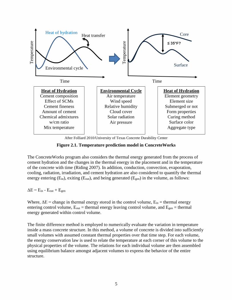
ConcreteWorks utilizes the finite difference method to analyze the thermal development of mass
concrete elements. To complete the thermal analysis of a mass concrete member, the software
considers the material constituents, mix proportion, geometry, formwork type, and
environmental conditions (Meeks and Folliard 2013) as shown in Figure 2.1.
5
After Folliard 2010/University of Texas Concrete Durability Center
Figure 2.1. Temperature prediction model in ConcreteWorks
The ConcreteWorks program also considers the thermal energy generated from the process of
cement hydration and the changes in the thermal energy in the placement and in the temperature
of the concrete with time (Riding 2007). In addition, conduction, convection, evaporation,
cooling, radiation, irradiation, and cement hydration are also considered to quantify the thermal
energy entering (Ein), exiting (Eout), and being generated (Egen) in the volume, as follows:
ΔE = Ein - Eout + Egen
Where, ΔE = change in thermal energy stored in the control volume, Ein = thermal energy
entering control volume, Eout = thermal energy leaving control volume, and Egen = thermal
energy generated within control volume.
The finite difference method is employed to numerically evaluate the variation in temperature
inside a mass concrete structure. In this method, a volume of concrete is divided into sufficiently
small volumes with assumed constant thermal properties over that time step. For each volume,
the energy conservation law is used to relate the temperature at each corner of this volume to the
physical properties of the volume. The relations for each individual volume are then assembled
using equilibrium balance amongst adjacent volumes to express the behavior of the entire
structure.
Heat of hydration
Environmental cycle
Heat transfer
Time
Tem
per
atu
re
≤ 35°F?
Core
Surface
Tem
per
ature
Time
Heat of Hydration
Cement composition
Effect of SCMs
Cement fineness
Amount of cement
Chemical admixtures
w/cm ratio
Mix temperature
Environmental Cycle
Air temperature
Wind speed
Relative humidity
Cloud cover
Solar radiation
Air pressure
Heat of Hydration
Element geometry
Element size
Submerged or not
Form properties
Curing method
Surface color
Aggregate type
6
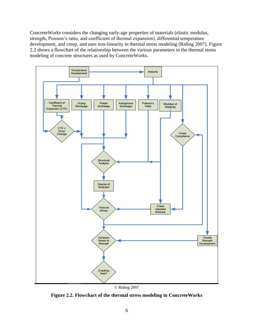
ConcreteWorks considers the changing early-age properties of materials (elastic modulus,
strength, Poisson’s ratio, and coefficient of thermal expansion), differential temperature
development, and creep, and uses non-linearity in thermal stress modeling (Riding 2007). Figure
2.2 shows a flowchart of the relationship between the various parameters in the thermal stress
modeling of concrete structures as used by ConcreteWorks.
© Riding 2007
Figure 2.2. Flowchart of the thermal stress modeling in ConcreteWorks
7
In order to calculate the thermal stresses, the concrete member degree of hydration (DOH) and
temperature development is first calculated. Next, the DOH and temperature development is used
to calculate the strains the concrete would undergo in case of a restraint, including the changing
early-age properties. After that, the concrete elastic stress is calculated from the free shrinkage
strains and mechanical properties by performing a structural analysis. Stress relaxation is then
applied to the concrete elastic stress. Finally, a failure criterion, such as the stress to tensile
strength ratio, is used to determine the cracking risk (Riding et al. 2017).
The software has a built-in statistical predictive model to calculate the variables needed to
perform the calculations. Some examples include a built-in 30-year historical weather model, the
use of cement chemistry typical of the cement type, the ability to calculate hydration parameters
from the cement chemistry, and, finally, the model for calculating heat transfer constants based
on aggregate classification.
In all cases, the program allows the user to overwrite programmatically determined values with
those obtained from laboratory testing. Doing so improves the overall accuracy of the resulting
temperature prediction (Meeks and Folliard 2013).
In the previous Iowa Mass Concrete for Bridge Foundations Study that Iowa State University’s
Institute for Transportation (InTrans) conducted for the Iowa DOT, the ConcreteWorks program
was used to study the temperature development profile in the concrete placed for the WB I-80
and US 34 bridge over the Missouri River in Iowa (Shaw et al. 2014). The results indicated that
the program is capable of predicting the maximum temperature and maximum temperature
difference of placements as well as the thermal development of placements at discrete locations
with regard to time to a reasonable degree. The project report concludes that, on average,
ConcreteWorks underestimates the maximum temperature of a placement by 12.3°F, and
overestimates the maximum temperature difference by 1.9°F. The researchers recommended
some adjustments to the inputs and outputs to ensure that the results are conservative and to
increase the analysis duration from 14 days to 30 days (Shaw et al. 2014).
4C-Temp&Stress Review
4C-Temp & Stress is a finite element (FE) computer program developed by the Danish
Technological Institute to conduct thermal, maturity, and stress analysis for concrete structures.
The software automatically transforms the physical concrete structure defined by the user into
formulations operated by using a finite element method. A set of triangular plane elements
representing the defined geometry is used to compute the temperature and stress following a
quadratic variation. The software calculates the time-dependent concrete temperatures and the
corresponding thermal stresses considering the influence of other significant parameters on the
thermal state of concrete. These are the parameters used: heat of hydration, thermal boundary
conditions, time of casting, heating wires or cooling pipes, and environmental factors (wind and
radiation). The numerical simulations provided by this software help to obtain the temperatures
that typically develop due to hydration of cement in concrete and, therefore, assist in planning
concrete casting in order to reduce the risk of cracks induced from thermal stresses.
8
The software’s development of temperatures and stresses are obtained from transient analysis,
i.e., as a function of place and time. When conducting thermal analysis, the external temperature,
type of insulation, internal heat generation by the materials, and the thermal boundary conditions,
all reflect necessary inputs for successful analysis. These latter inputs along with external loads
and supports, thermal expansion, stiffness and strength properties developed as a function of
maturity, and creep and relaxation of materials are also considered necessary for subsequent
stress analysis. It is noteworthy to mention that stress analysis is typically performed based on
inputs given for thermal analysis and its corresponding results. However, if the interest is on
evaluating stresses without considering the thermal impact, the stress analysis will be based on
external loads only.
The software uses certain computational assumptions to simplify the numerical simulations,
particularly on those employed in the thermal analysis. For example, the location of the
minimum temperature is considered as that at the top surface of the concrete structure, and the
maximum temperature is considered as that at mid-center. The top surface temperature is
considered as an ambient temperature, which equals an averaged 7-day temperature and is
defined through a sinusoidal curve during the entire duration of the analysis. This sinusoidal
curve assumes a constant wind speed instead of actual weather conditions, where the temperature
history varies and differs from one day to another. The definition of the temperature difference is
that between the location of mid-center and the top surface sensor located three inches below the
surface. Another default input assumption is on the nonlinear convergence criteria that are
typically defined as 0.001. This convergence value deems large for nonlinear calculations. Thus,
it is advised to reduce this value at the start of the analysis further, and if convergence problems
occur, the limit can be increased accordingly.
The 4C software consists of three major workspaces: Project Editor, Project Solver, and Result
Viewer. Project Editor is where parts of the project like concrete geometry, calculation
parameters, and mix-material database are defined. In this workspace, the concrete geometry is
drawn, and the boundary conditions along with construction insulations are assigned. Further, a
proper concrete mix design is established and specified to the desired geometry. Once the latter
is carried out, the next step would be transforming the concrete geometry to finite element
formulations by generating triangular mesh distributions. This step is done under the Project
Solver workspace. The default values can be used for the mesh size. Users also have the option
to modify the mesh sizes. Subsequently, the analysis is conducted, and the results can be viewed
in the Results Viewer workspace. The results of the analysis are displayed either in x-y diagrams
or as isocurves. At any specified time and place after casting, the results can be presented. The
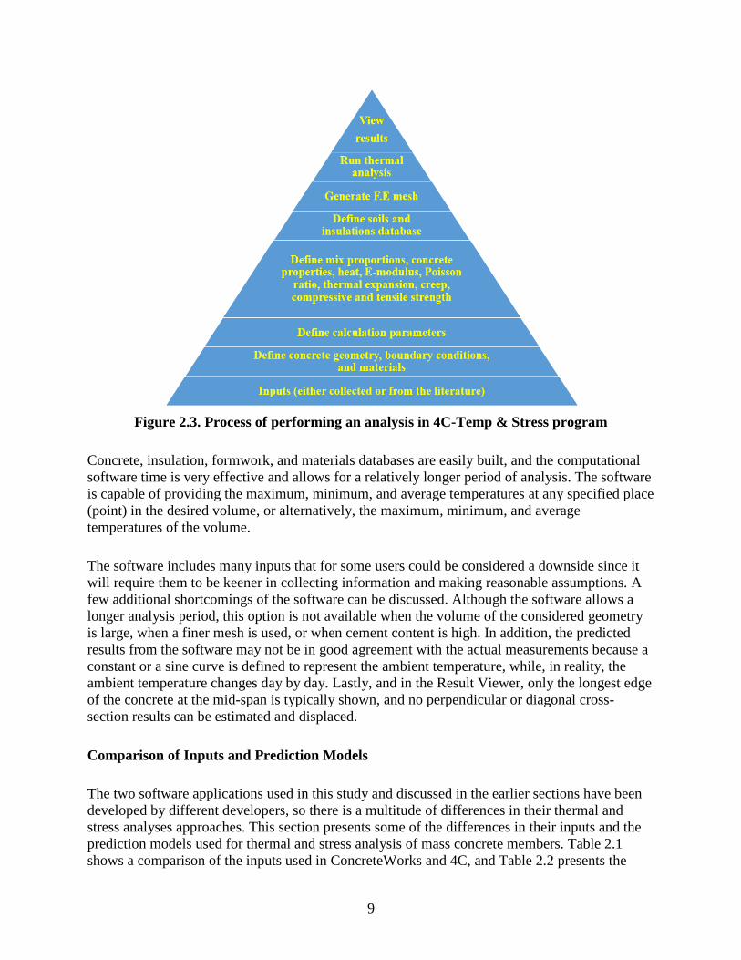
major steps in the above-discussed workspaces are illustrated in Figure 2.3.
9
Figure 2.3. Process of performing an analysis in 4C-Temp & Stress program
Concrete, insulation, formwork, and materials databases are easily built, and the computational
software time is very effective and allows for a relatively longer period of analysis. The software
is capable of providing the maximum, minimum, and average temperatures at any specified place
(point) in the desired volume, or alternatively, the maximum, minimum, and average
temperatures of the volume.
The software includes many inputs that for some users could be considered a downside since it
will require them to be keener in collecting information and making reasonable assumptions. A
few additional shortcomings of the software can be discussed. Although the software allows a
longer analysis period, this option is not available when the volume of the considered geometry
is large, when a finer mesh is used, or when cement content is high. In addition, the predicted
results from the software may not be in good agreement with the actual measurements because a
constant or a sine curve is defined to represent the ambient temperature, while, in reality, the
ambient temperature changes day by day. Lastly, and in the Result Viewer, only the longest edge
of the concrete at the mid-span is typically shown, and no perpendicular or diagonal cross-
section results can be estimated and displaced.
Comparison of Inputs and Prediction Models
The two software applications used in this study and discussed in the earlier sections have been
developed by different developers, so there is a multitude of differences in their thermal and
stress analyses approaches. This section presents some of the differences in their inputs and the
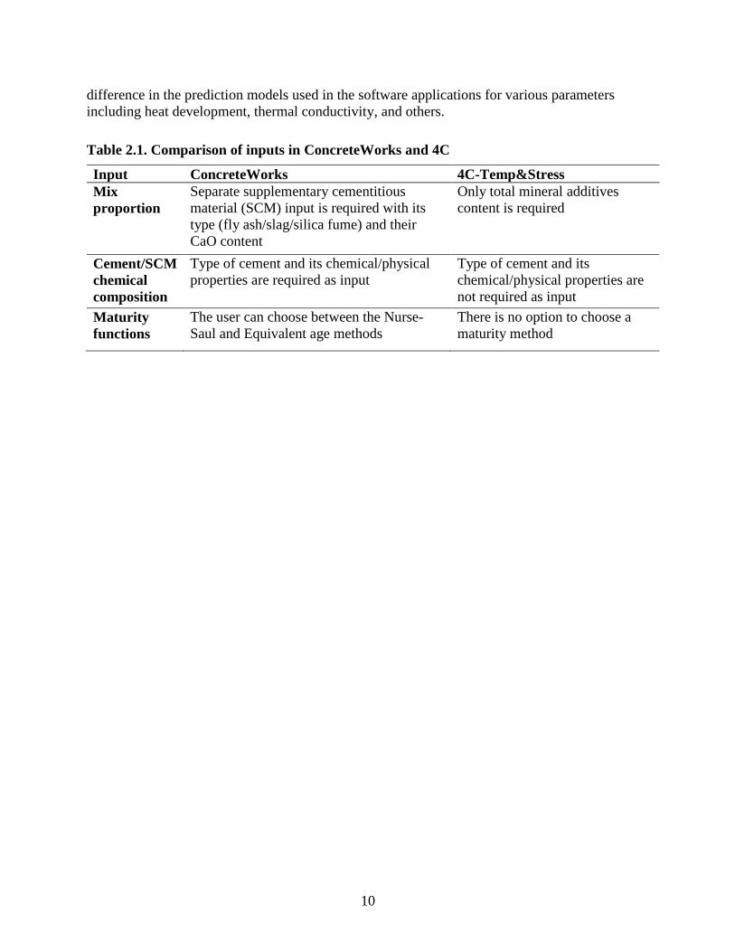
prediction models used for thermal and stress analysis of mass concrete members. Table 2.1
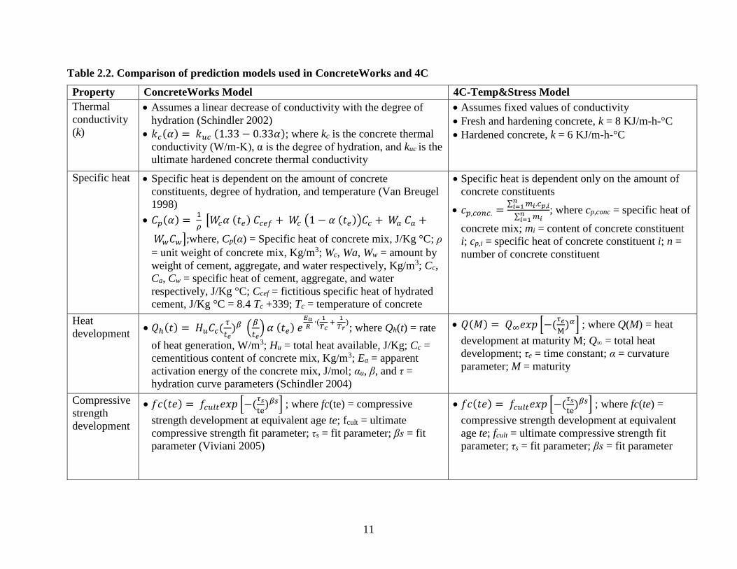
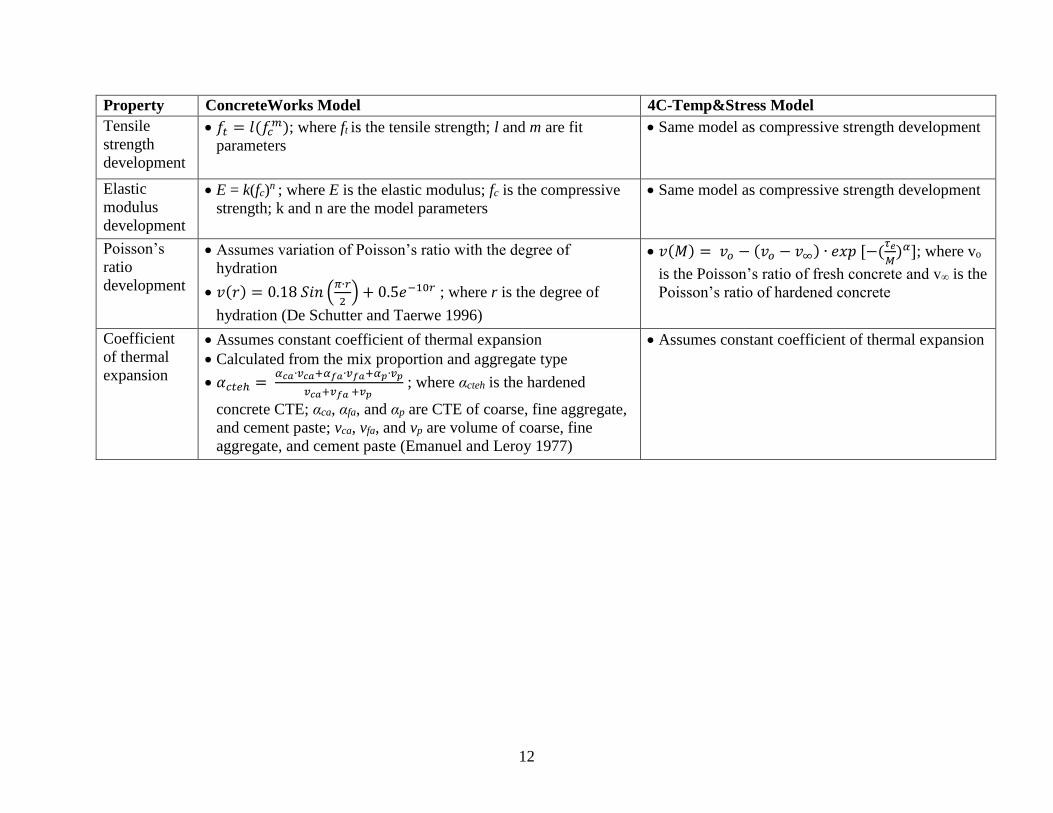
shows a comparison of the inputs used in ConcreteWorks and 4C, and Table 2.2 presents the
10
difference in the prediction models used in the software applications for various parameters
including heat development, thermal conductivity, and others.
Table 2.1. Comparison of inputs in ConcreteWorks and 4C
Input ConcreteWorks 4C-Temp&Stress
Mix
proportion
Separate supplementary cementitious
material (SCM) input is required with its
type (fly ash/slag/silica fume) and their
CaO content
Only total mineral additives
content is required
Cement/SCM
chemical
composition
Type of cement and its chemical/physical
properties are required as input
Type of cement and its
chemical/physical properties are
not required as input
Maturity
functions
The user can choose between the Nurse-
Saul and Equivalent age methods
There is no option to choose a
maturity method
11
Table 2.2. Comparison of prediction models used in ConcreteWorks and 4C
Property ConcreteWorks Model 4C-Temp&Stress Model
Thermal
conductivity
(k)
Assumes a linear decrease of conductivity with the degree of
hydration (Schindler 2002)
𝑘𝑐(𝛼) = 𝑘𝑢𝑐 (1.33 − 0.33𝛼); where kc is the concrete thermal
conductivity (W/m-K), α is the degree of hydration, and kuc is the
ultimate hardened concrete thermal conductivity
Assumes fixed values of conductivity
Fresh and hardening concrete, k = 8 KJ/m-h-°C
Hardened concrete, k = 6 KJ/m-h-°C
Specific heat Specific heat is dependent on the amount of concrete
constituents, degree of hydration, and temperature (Van Breugel
1998)
𝐶𝑝(𝛼) = 1
𝜌 [𝑊𝑐𝛼 (𝑡𝑒) 𝐶𝑐𝑒𝑓 + 𝑊𝑐 (1 − 𝛼 (𝑡𝑒))𝐶𝑐 + 𝑊𝑎 𝐶𝑎 +
𝑊𝑤𝐶𝑤];where, Cp(α) = Specific heat of concrete mix, J/Kg °C; ρ
= unit weight of concrete mix, Kg/m3; Wc, Wa, Ww = amount by
weight of cement, aggregate, and water respectively, Kg/m3; Cc,
Ca, Cw = specific heat of cement, aggregate, and water
respectively, J/Kg °C; Ccef = fictitious specific heat of hydrated
cement, J/Kg °C = 8.4 Tc +339; Tc = temperature of concrete
Specific heat is dependent only on the amount of
concrete constituents
𝑐𝑝,𝑐𝑜𝑛𝑐. =∑ 𝑚𝑖.𝑐𝑝,𝑖
𝑛𝑖=1
∑ 𝑚𝑖𝑛𝑖=1
; where cp,conc = specific heat of
concrete mix; mi = content of concrete constituent
i; cp,i = specific heat of concrete constituent i; n =
number of concrete constituent
Heat
development 𝑄ℎ(𝑡) = 𝐻𝑢𝐶𝑐(
𝜏
𝑡𝑒)𝛽 (
𝛽
𝑡𝑒) 𝛼 (𝑡𝑒) 𝑒
𝐸𝑎𝑅
∙(1
𝑇𝑐 +
1
𝑇𝑟); where Qh(t) = rate
of heat generation, W/m3; Hu = total heat available, J/Kg; Cc =
cementitious content of concrete mix, Kg/m3; Ea = apparent
activation energy of the concrete mix, J/mol; αu, β, and τ =
hydration curve parameters (Schindler 2004)
𝑄(𝑀) = 𝑄∞𝑒𝑥𝑝 [−(𝜏𝑒
M)𝛼] ; where Q(M) = heat
development at maturity M; Q∞ = total heat
development; τe = time constant; α = curvature
parameter; M = maturity
Compressive
strength
development
𝑓𝑐(𝑡𝑒) = 𝑓𝑐𝑢𝑙𝑡𝑒𝑥𝑝 [−(𝜏𝑠
te)𝛽𝑠] ; where fc(te) = compressive
strength development at equivalent age te; fcult = ultimate
compressive strength fit parameter; τs = fit parameter; βs = fit
parameter (Viviani 2005)
𝑓𝑐(𝑡𝑒) = 𝑓𝑐𝑢𝑙𝑡𝑒𝑥𝑝 [−(𝜏𝑠
te)𝛽𝑠] ; where fc(te) =
compressive strength development at equivalent
age te; fcult = ultimate compressive strength fit
parameter; τs = fit parameter; βs = fit parameter
12
Property ConcreteWorks Model 4C-Temp&Stress Model
Tensile
strength
development
𝑓𝑡 = 𝑙(𝑓𝑐𝑚); where ft is the tensile strength; l and m are fit
parameters
Same model as compressive strength development
Elastic
modulus
development
E = k(fc)n ; where E is the elastic modulus; fc is the compressive
strength; k and n are the model parameters
Same model as compressive strength development
Poisson’s
ratio
development
Assumes variation of Poisson’s ratio with the degree of
hydration
𝑣(𝑟) = 0.18 𝑆𝑖𝑛 (𝜋∙𝑟
2) + 0.5𝑒−10𝑟 ; where r is the degree of
hydration (De Schutter and Taerwe 1996)
𝑣(𝑀) = 𝑣𝑜 − (𝑣𝑜 − 𝑣∞) ∙ 𝑒𝑥𝑝 [−(𝜏𝑒
𝑀)𝛼]; where vo
is the Poisson’s ratio of fresh concrete and v∞ is the
Poisson’s ratio of hardened concrete
Coefficient
of thermal
expansion
Assumes constant coefficient of thermal expansion
Calculated from the mix proportion and aggregate type
𝛼𝑐𝑡𝑒ℎ = 𝛼𝑐𝑎∙𝑣𝑐𝑎+𝛼𝑓𝑎∙𝑣𝑓𝑎+𝛼𝑝∙𝑣𝑝
𝑣𝑐𝑎+𝑣𝑓𝑎 +𝑣𝑝 ; where αcteh is the hardened
concrete CTE; αca, αfa, and αp are CTE of coarse, fine aggregate,
and cement paste; vca, vfa, and vp are volume of coarse, fine
aggregate, and cement paste (Emanuel and Leroy 1977)
Assumes constant coefficient of thermal expansion
13
3. EXPERIMENTS AND TEST METHODS
The default input data in ConcreteWorks were to be calibrated with those of the commonly used
concrete mixtures for Iowa mass concrete construction. Various tests were performed on these
mixes in the Portland Cement Concrete (PCC) Pavement and Materials Research Laboratory at
Iowa State University. Test methods and experiments are discussed in the following sections.
Materials and Mixes
Four different concrete mixes were tested in the laboratory for their mechanical and thermal
properties. The mixes commonly used for mass concrete construction in Iowa were selected for
this study based on advice from the technical advisory committee (TAC). Four different types of
cement—Type I, IP (25), IS (20), and I/II—and two types of supplementary cementitious
materials (SCMs)—Class C fly ash and ground-granulated blast-furnace slag (GGBFS)—were
used. Type IP (25) cement includes 25% Class F fly ash and Type IS (20) includes 20% Grade
120 slag. All four concrete mixes had a 20% replacement of cement by Class C fly ash, while
Mix 4 had an additional replacement of cement by 30% with Grade 100 GGBFS. The fine-to-
coarse aggregate ratio was selected as 50:50 and a water-binder ratio of 0.43 was used for all of
the mixes. The mix proportions (with constituent materials in pounds per cubic yard of concrete)
are presented in Table 3.1.
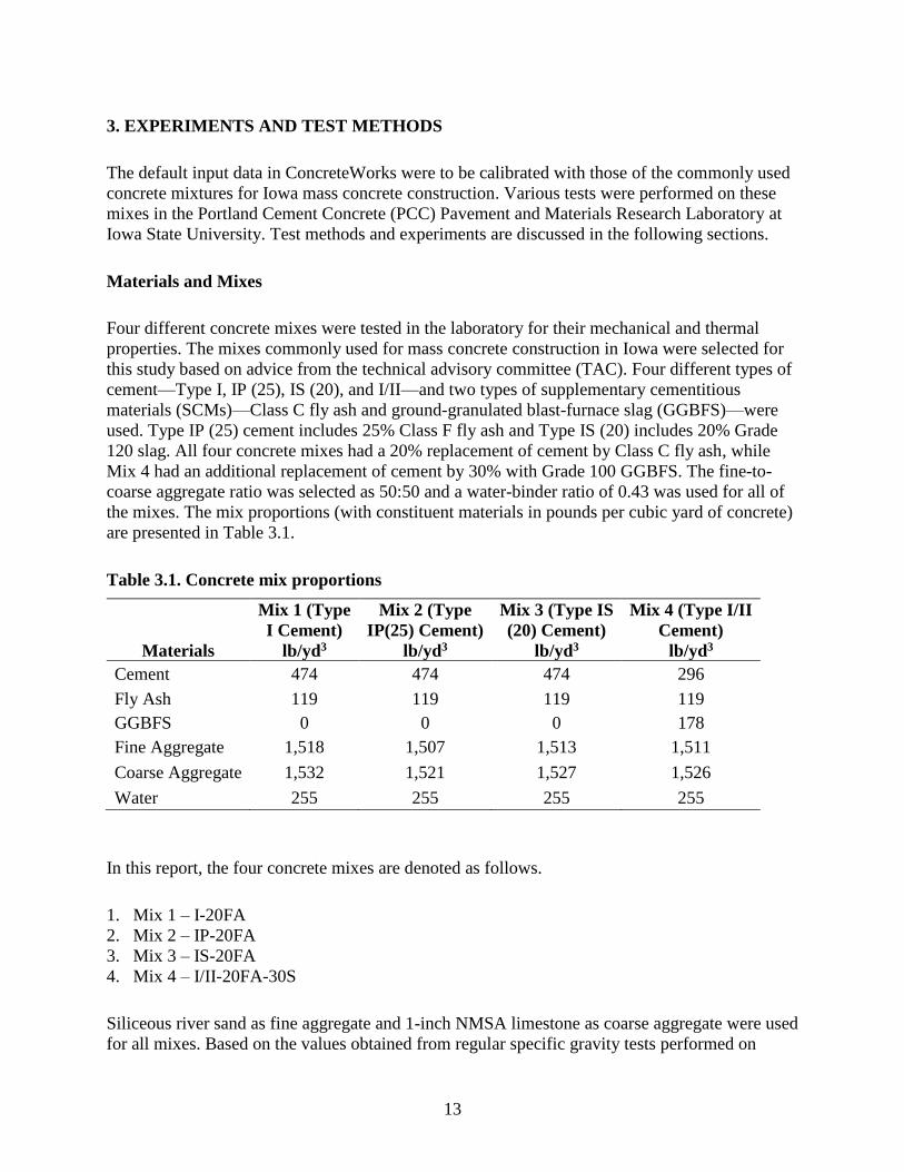
Table 3.1. Concrete mix proportions
Materials
Mix 1 (Type
I Cement)
lb/yd3
Mix 2 (Type
IP(25) Cement)
lb/yd3
Mix 3 (Type IS
(20) Cement)
lb/yd3
Mix 4 (Type I/II
Cement)
lb/yd3
Cement 474 474 474 296
Fly Ash 119 119 119 119
GGBFS 0 0 0 178
Fine Aggregate 1,518 1,507 1,513 1,511
Coarse Aggregate 1,532 1,521 1,527 1,526
Water 255 255 255 255
In this report, the four concrete mixes are denoted as follows.
1. Mix 1 – I-20FA
2. Mix 2 – IP-20FA
3. Mix 3 – IS-20FA
4. Mix 4 – I/II-20FA-30S
Siliceous river sand as fine aggregate and 1-inch NMSA limestone as coarse aggregate were used
for all mixes. Based on the values obtained from regular specific gravity tests performed on
14
aggregate batches, mix proportions were modified accordingly for the variation in specific
gravity values. The following sections present the properties of the materials used.
Cementitious Materials
Concrete mixes contained different cementitious materials as outlined previously. Different types
of cement were used. ASTM C618 Class C fly ash was used in all four mixes with 20%
replacement of cement, while Mix 4 had an additional 30% replacement of cement by GGBFS.
Material data sheets were provided by the manufacturer showing the chemical composition of
the material and also the physical properties. Table 3.2 shows the chemical compositions of all of
the cementitious materials.
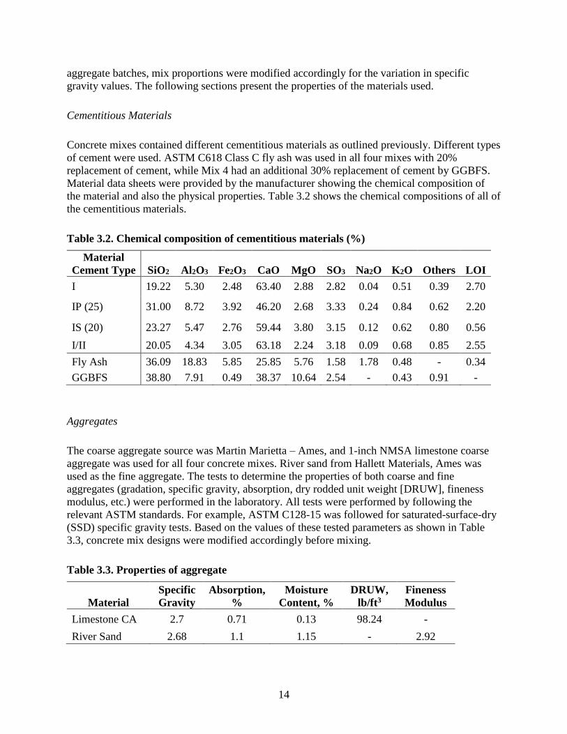
Table 3.2. Chemical composition of cementitious materials (%)
Material
Cement Type SiO2 Al2O3 Fe2O3 CaO MgO SO3 Na2O K2O Others LOI
I 19.22 5.30 2.48 63.40 2.88 2.82 0.04 0.51 0.39 2.70
IP (25) 31.00 8.72 3.92 46.20 2.68 3.33 0.24 0.84 0.62 2.20
IS (20) 23.27 5.47 2.76 59.44 3.80 3.15 0.12 0.62 0.80 0.56
I/II 20.05 4.34 3.05 63.18 2.24 3.18 0.09 0.68 0.85 2.55
Fly Ash 36.09 18.83 5.85 25.85 5.76 1.58 1.78 0.48 - 0.34
GGBFS 38.80 7.91 0.49 38.37 10.64 2.54 - 0.43 0.91 -
Aggregates
The coarse aggregate source was Martin Marietta – Ames, and 1-inch NMSA limestone coarse
aggregate was used for all four concrete mixes. River sand from Hallett Materials, Ames was
used as the fine aggregate. The tests to determine the properties of both coarse and fine
aggregates (gradation, specific gravity, absorption, dry rodded unit weight [DRUW], fineness
modulus, etc.) were performed in the laboratory. All tests were performed by following the
relevant ASTM standards. For example, ASTM C128-15 was followed for saturated-surface-dry
(SSD) specific gravity tests. Based on the values of these tested parameters as shown in Table
3.3, concrete mix designs were modified accordingly before mixing.
Table 3.3. Properties of aggregate
Material
Specific
Gravity
Absorption,
%
Moisture
Content, %
DRUW,
lb/ft3
Fineness
Modulus
Limestone CA 2.7 0.71 0.13 98.24 -
River Sand 2.68 1.1 1.15 - 2.92
15
The specific gravity of sand and coarse aggregate were 2.68 and 2.7, respectively. The DRUW of
limestone aggregate was measured to be 98.24 lb/ft3 and the fineness modulus of sand was
determined to be 2.92.
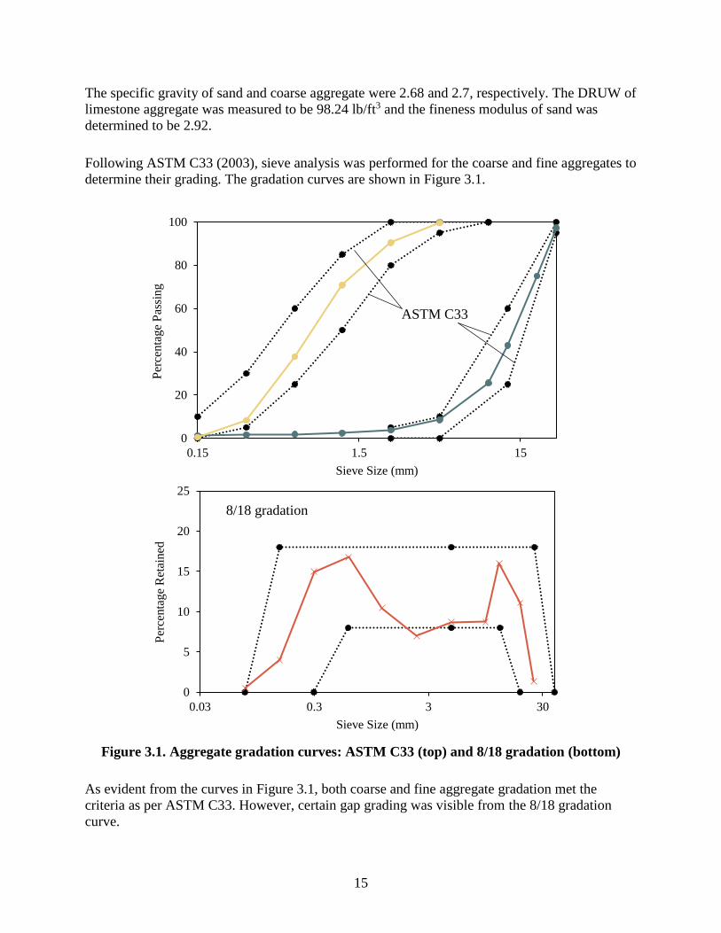
Following ASTM C33 (2003), sieve analysis was performed for the coarse and fine aggregates to
determine their grading. The gradation curves are shown in Figure 3.1.
Figure 3.1. Aggregate gradation curves: ASTM C33 (top) and 8/18 gradation (bottom)
As evident from the curves in Figure 3.1, both coarse and fine aggregate gradation met the
criteria as per ASTM C33. However, certain gap grading was visible from the 8/18 gradation
curve.
0
20
40
60
80
100
0.15 1.5 15
Per
centa
ge
Pas
sin
g
Sieve Size (mm)
ASTM C33
0
5
10
15
20
25
0.03 0.3 3 30
Per
centa
ge
Ret
ained
Sieve Size (mm)
8/18 gradation
16
Chemical Admixtures
A low range water reducer (LRWR), BASF MasterPozzolith 322N, was used in sample
comparison testing. As recommended by the manufacturer and the Iowa DOT, the dosage was
kept to 3 fl oz. per 100 lbs. of cementitious materials. An air-entraining admixture (AEA),
DARAVAIR 100, was also used. As recommended, the dosage was kept to 1 fl oz. per 100 lbs.
of cementitious materials.
Tests and Methods
Fresh Properties
Concrete mixes were prepared using a drum mixer in the laboratory. Properties of fresh concrete
such as slump, air content, and unit weight were then tested by following the standard test
procedures per ASTM C143/C143M (2015), ASTM C231/231M (2010), and ASTM
C138/C138M-13, respectively.
Mechanical Properties
As required by the ConcreteWorks program, the mechanical properties of the four concrete
mixes were tested in the laboratory as follows.
Compressive Strength
Compressive strength tests were performed on 4×8 in. cylindrical specimens as per the ASTM
C39 (2016) test procedure. The Test Mark Industries testing apparatus available in the laboratory
was used for this purpose. Three specimens of each mix were moist-cured at 74°F and tested at
curing ages of 1, 3, 7, 14, and 28 days.
Split Tensile Strength
The test for split tensile strength of concrete mixes was performed on 28-day moistcured 4×8 in.
cylindrical specimens following the ASTM C496 (2011) test procedure. Three specimens were
tested for each mix and the mean was taken as the split tensile strength of the concrete mix.
Elastic Modulus
The static modulus of elasticity of the concrete mixes in compression was also tested using 28-
day moist-cured 4×8 in. cylindrical specimens following the ASTM C469/C469M (2014) test
procedure.
17
Maturity
The maturity method is a technique for estimating concrete strength based on the assumption that
samples of a given concrete mixture attain equal strengths if they attain an equal value of the
maturity index. The maturity index is an indicator of maturity that is calculated from the
temperature history of the cementitious mixture by using a maturity function ASTM C1074
(2015).
As per ASTM C1074, there are two methods for the computing maturity index from the
measured temperature history of concrete:
Nurse-Saul
Equivalent age
Because of its simplicity, the Nurse-Saul method is frequently used in the field, and it is for this
reason that this method was used for this investigation.
The temperature-time factor is calculated as follows:
𝑀 (𝑡) = ∑(𝑇𝑎 – 𝑇𝑜) 𝛥𝑡 (1)
Where M (t) is the temperature-time factor at age t (in °F –hours), Δ𝑡 is the time interval (in
hours), Ta is the average concrete temperature during time interval Δ𝑡, and To is the datum
temperature (in °F). Following the ASTM C39 (2016) standard procedure, 23 4×8 in. cylindrical
specimens were prepared as per the mixture proportions for each of the four mixes. iButton
temperature sensors were embedded in two specimens and all the specimens were moist-cured in
a temperature and humidity controlled room at 74°F. The temperature of the concrete specimens
was recorded at an interval of 45 minutes. Three specimens of each mix were tested at 1, 3, 7, 14,
28, 56, and 90 days for compressive strength as per ASTM C39 (2016). At each test age, the
temperature-time factor (TTF) was calculated using a datum temperature of 14°F, and
compressive strength was plotted as a function of TTF. The compressive strength-maturity
relationship for each mix was then developed by performing a regression analysis to determine a
best-fit equation to the data. The best-fit equation for all of the mixes was found to be of the form
where compressive strength is a linear function of the logarithm of maturity index (in this case
TTF) as given in equation (2).
S = a + b log (M) (2)
Where S is the compressive strength (in psi), M is the maturity index (TTF), and a and b are
coefficients. The ConcreteWorks program allows the user to choose between two methods
(Nurse-Saul and equivalent age) for computing the maturity index. Based on the selected
method, relevant parameters can be edited. For example, values of the coefficients a and b can be
entered manually if the Nurse-Saul method is selected for maturity calculations.
18
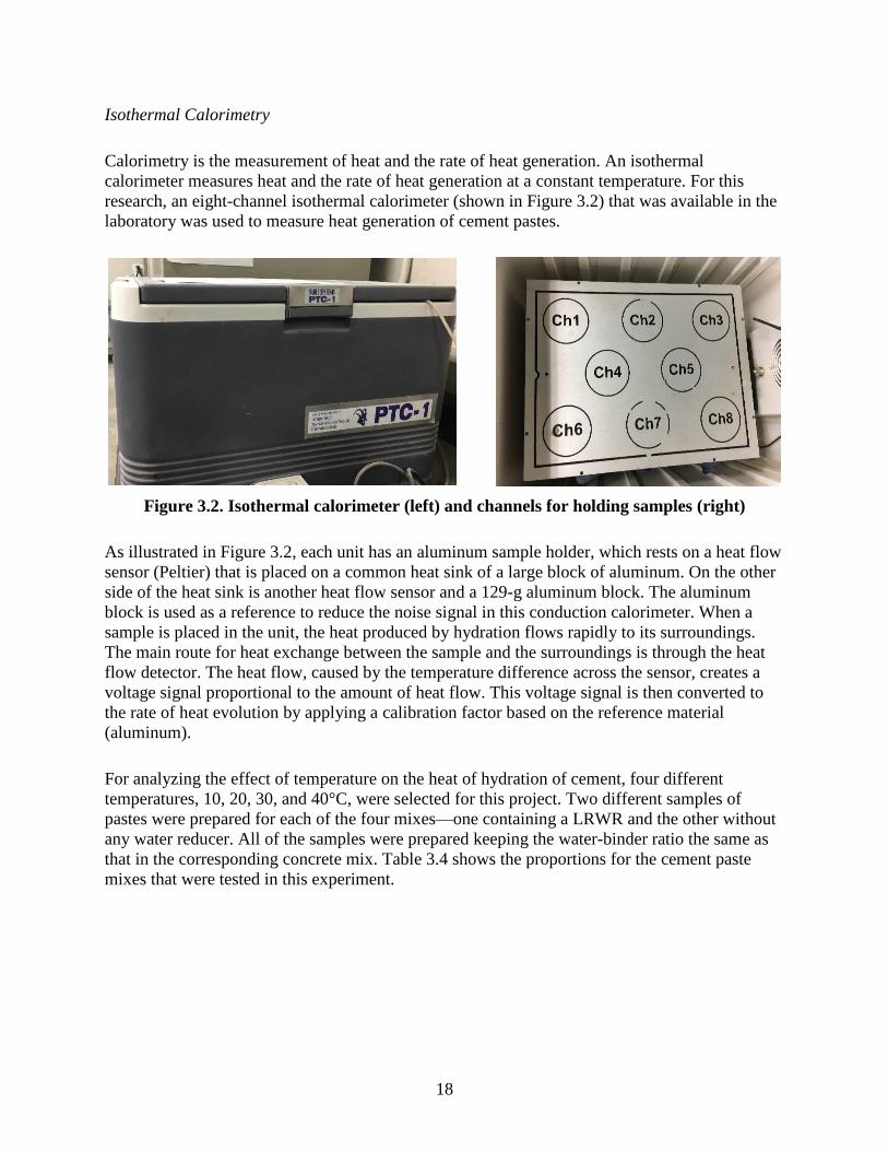
Isothermal Calorimetry
Calorimetry is the measurement of heat and the rate of heat generation. An isothermal
calorimeter measures heat and the rate of heat generation at a constant temperature. For this
research, an eight-channel isothermal calorimeter (shown in Figure 3.2) that was available in the
laboratory was used to measure heat generation of cement pastes.
Figure 3.2. Isothermal calorimeter (left) and channels for holding samples (right)
As illustrated in Figure 3.2, each unit has an aluminum sample holder, which rests on a heat flow
sensor (Peltier) that is placed on a common heat sink of a large block of aluminum. On the other
side of the heat sink is another heat flow sensor and a 129-g aluminum block. The aluminum
block is used as a reference to reduce the noise signal in this conduction calorimeter. When a
sample is placed in the unit, the heat produced by hydration flows rapidly to its surroundings.
The main route for heat exchange between the sample and the surroundings is through the heat
flow detector. The heat flow, caused by the temperature difference across the sensor, creates a
voltage signal proportional to the amount of heat flow. This voltage signal is then converted to
the rate of heat evolution by applying a calibration factor based on the reference material
(aluminum).
For analyzing the effect of temperature on the heat of hydration of cement, four different
temperatures, 10, 20, 30, and 40°C, were selected for this project. Two different samples of
pastes were prepared for each of the four mixes—one containing a LRWR and the other without
any water reducer. All of the samples were prepared keeping the water-binder ratio the same as
that in the corresponding concrete mix. Table 3.4 shows the proportions for the cement paste
mixes that were tested in this experiment.
19
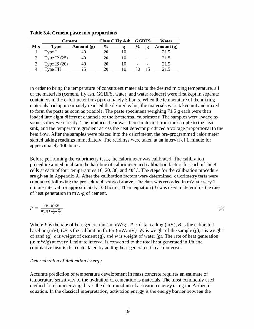
Table 3.4. Cement paste mix proportions
Mix
Cement Class C Fly Ash GGBFS Water
Type Amount (g) % g % g Amount (g)
1 Type I 40 20 10 - - 21.5
2 Type IP (25) 40 20 10 - - 21.5
3 Type IS (20) 40 20 10 - - 21.5
4 Type I/II 25 20 10 30 15 21.5
In order to bring the temperature of constituent materials to the desired mixing temperature, all
of the materials (cement, fly ash, GGBFS, water, and water reducer) were first kept in separate
containers in the calorimeter for approximately 5 hours. When the temperature of the mixing
materials had approximately reached the desired value, the materials were taken out and mixed
to form the paste as soon as possible. The paste specimens weighing 71.5 g each were then
loaded into eight different channels of the isothermal calorimeter. The samples were loaded as
soon as they were ready. The produced heat was then conducted from the sample to the heat
sink, and the temperature gradient across the heat detector produced a voltage proportional to the
heat flow. After the samples were placed into the calorimeter, the pre-programmed calorimeter
started taking readings immediately. The readings were taken at an interval of 1 minute for
approximately 100 hours.
Before performing the calorimetry tests, the calorimeter was calibrated. The calibration
procedure aimed to obtain the baseline of calorimeter and calibration factors for each of the 8
cells at each of four temperatures 10, 20, 30, and 40°C. The steps for the calibration procedure
are given in Appendix A. After the calibration factors were determined, calorimetry tests were
conducted following the procedure discussed above. The data was recorded in mV at every 1-
minute interval for approximately 100 hours. Then, equation (3) was used to determine the rate
of heat generation in mW/g of cement.
𝑃 = (𝑅−𝐵)𝐶𝐹
𝑊𝑠/(1+𝑠
𝑐+
𝑤
𝑐 ) (3)
Where P is the rate of heat generation (in mW/g), R is data reading (mV), B is the calibrated
baseline (mV), CF is the calibration factor (mW/mV), Ws is weight of the sample (g), s is weight
of sand (g), c is weight of cement (g), and w is weight of water (g). The rate of heat generation
(in mW/g) at every 1-minute interval is converted to the total heat generated in J/h and
cumulative heat is then calculated by adding heat generated in each interval.
Determination of Activation Energy
Accurate prediction of temperature development in mass concrete requires an estimate of
temperature sensitivity of the hydration of cementitious materials. The most commonly used
method for characterizing this is the determination of activation energy using the Arrhenius
equation. In the classical interpretation, activation energy is the energy barrier between the

20
reactant and product for a single reaction system. Cementitious systems involve multiple
reactions that occur simultaneously, interact with each other, and change with time. The
measurement of Ea for cementitious systems represents a globally averaged temperature
sensitivity of the mixture; this empirically determined value is often referred to as the “apparent”
activation energy (Riding et al. 2011). The modified ASTM C1074 procedure (Poole et al. 2007)
was adopted here for determination of apparent activation energy.
Degree of hydration (DOH) of cementitious material at a specific time, t, is determined by taking
the ratio of heat evolved at time t to the total amount of heat available as follows.
𝛼(𝑡) = 𝐻 (𝑡)
𝐻𝑢 (4)
Where α(t) is the degree of hydration at time t, H(t) is cumulative heat of hydration from time 0
to t (J/g), and Hu is total heat available for reaction (J/g).
Total heat available for reaction, Hu, is calculated from the material components and chemical
compositions as follows.
𝐻𝑢 = 𝐻𝑐𝑒𝑚 ∙ 𝑝𝑐𝑒𝑚 + 461 ∙ 𝑝𝑠𝑙𝑎𝑔 + 1800 ∙ 𝑝𝐹𝐴−𝐶𝑎𝑂 ∙ 𝑝𝐹𝐴 (5)
𝐻𝑐𝑒𝑚 = 500 ∙ 𝑝𝐶3𝑆 + 260 ∙ 𝑝𝐶2𝑆 + 866 ∙ 𝑝𝐶3𝐴 + 420 ∙ 𝑝𝐶4𝐴𝐹 + 624 ∙ 𝑝𝑆𝑂3 + 1186 ∙ 𝑝𝐹𝑟𝑒𝑒𝐶𝑎 + 850 ∙ 𝑝𝑀𝑔𝑂 (6)
Where Hcem is heat of hydration of cement (J/g), Pcem is cement mass to total cementitious
content ratio, Pslag is slag mass to total cementitious content ratio, PFA-CaO is fly ash CaO mass to
total fly ash content ratio, PFA is fly ash mass to total cementitious content ratio, PC3S, PC2S, PC3A,
PC4AF, PSO3, PFreeCa, and PMgO are the cement composition-total cement content weight ratios.
As suggested by a number of researchers, an exponential function can be used to characterize
cement hydration based on the degree of hydration data. The most commonly used relationship is
a three-parameter model given below.
𝛼 (𝑡) = 𝛼𝑢 ∙ 𝑒− [
𝜏
𝑡
𝛽] (7)
Where α (t) is the degree of hydration at time, t, αu is the ultimate degree of hydration, β is the
hydration shape parameter, and τ is the hydration time parameter (hours). αu, β, and τ in equation
(7) are three hydration curve parameters used to characterize DOH of cementitious materials. A
larger αu indicates a higher magnitude of ultimate DOH, and a larger τ implies a larger delay of
hydration. Since β represents the slope of the major linear part of the hydration shape, a larger β
implies a higher hydration rate at the linear portion of hydration curves.
21
The hydration curve parameters and the apparent activation energy are calculated according to
the modified ASTM C1074 procedure as outlined in Methods for Calculating Apparent
Activation Energy of Cementitious Systems (Poole et al. 2007). The steps of the calculation are
as follows:
1. The hydration curve parameters αu, β, and τ in equation (7) are fit using the least squares
approach for the cementitious system degree of hydration calculated from the cumulative
isothermal heat of the hydration curve at 20°C using equations (4) through (6) for a particular
concrete mix.
2. Following Step 1, parameters are fit at other temperatures, 10, 30, and 40°C as well. Since it
has been shown in the literature that the ultimate degree of hydration αu and shape parameter
β are independent of temperature, values of these two parameters at 10, 30, and 40°C are kept
equal to the values found at 20°C. The value of the hydration time parameter τ is changed for
each temperature to fit the cumulative isothermal heat of hydration values at each
temperature.
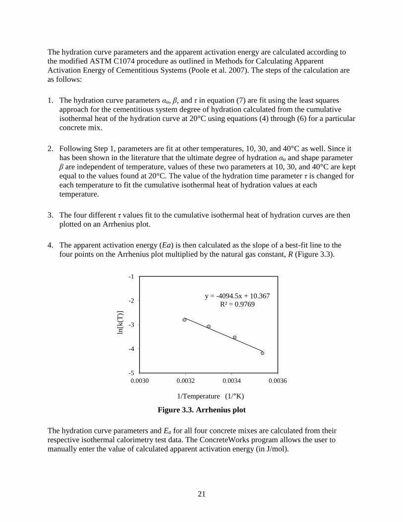
3. The four different τ values fit to the cumulative isothermal heat of hydration curves are then
plotted on an Arrhenius plot.
4. The apparent activation energy (Ea) is then calculated as the slope of a best-fit line to the
four points on the Arrhenius plot multiplied by the natural gas constant, R (Figure 3.3).
Figure 3.3. Arrhenius plot
The hydration curve parameters and Ea for all four concrete mixes are calculated from their
respective isothermal calorimetry test data. The ConcreteWorks program allows the user to
manually enter the value of calculated apparent activation energy (in J/mol).
y = -4094.5x + 10.367
R² = 0.9769
-5
-4
-3
-2
-1
0.0030 0.0032 0.0034 0.0036
ln[k
(T)]
1/Temperature (1/°K)
22
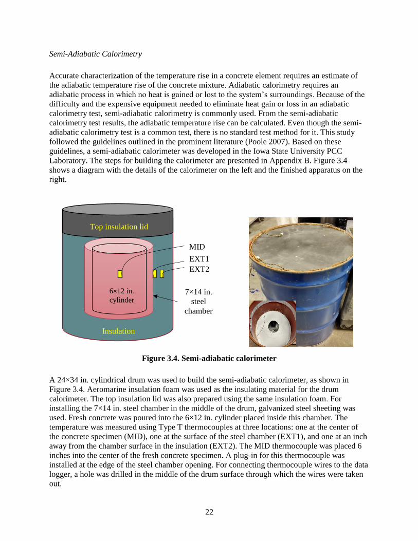
Semi-Adiabatic Calorimetry
Accurate characterization of the temperature rise in a concrete element requires an estimate of
the adiabatic temperature rise of the concrete mixture. Adiabatic calorimetry requires an
adiabatic process in which no heat is gained or lost to the system’s surroundings. Because of the
difficulty and the expensive equipment needed to eliminate heat gain or loss in an adiabatic
calorimetry test, semi-adiabatic calorimetry is commonly used. From the semi-adiabatic
calorimetry test results, the adiabatic temperature rise can be calculated. Even though the semi-
adiabatic calorimetry test is a common test, there is no standard test method for it. This study
followed the guidelines outlined in the prominent literature (Poole 2007). Based on these
guidelines, a semi-adiabatic calorimeter was developed in the Iowa State University PCC
Laboratory. The steps for building the calorimeter are presented in Appendix B. Figure 3.4
shows a diagram with the details of the calorimeter on the left and the finished apparatus on the
right.
Figure 3.4. Semi-adiabatic calorimeter
A 24×34 in. cylindrical drum was used to build the semi-adiabatic calorimeter, as shown in
Figure 3.4. Aeromarine insulation foam was used as the insulating material for the drum
calorimeter. The top insulation lid was also prepared using the same insulation foam. For
installing the 7×14 in. steel chamber in the middle of the drum, galvanized steel sheeting was
used. Fresh concrete was poured into the 6×12 in. cylinder placed inside this chamber. The
temperature was measured using Type T thermocouples at three locations: one at the center of
the concrete specimen (MID), one at the surface of the steel chamber (EXT1), and one at an inch
away from the chamber surface in the insulation (EXT2). The MID thermocouple was placed 6
inches into the center of the fresh concrete specimen. A plug-in for this thermocouple was
installed at the edge of the steel chamber opening. For connecting thermocouple wires to the data
logger, a hole was drilled in the middle of the drum surface through which the wires were taken
out.
6×12 in.
cylinder
EXT1
TC EXT2
TC
7×14 in.
steel
chamber
Top insulation lid
MID
Insulation
23
The test setup was kept in a closed room where temperature variations were limited. Concrete
specimens for each of four mixes were prepared as per ASTM C192 (2016) and placed in the
calorimeter as soon as possible. The data was recorded using a Pico Technology USB TC-08
data logger for 160 hours at 15-minute intervals. To measure the heat loss from the calorimeter,
it was calibrated before the test. The calibration procedure is covered in Appendix C.
Determination of Adiabatic Temperature Rise
After the determination of the calibration factors, the test was performed on each of four concrete
mixes one by one and their semi-adiabatic temperature data were recorded. It was required to
calculate the adiabatic temperature rise of the concrete mixture from the recorded semi-adiabatic
temperature data. Since no standard testing procedure is currently available, the steps outlined in
Hydration Study of Cementitious Materials using Semi-Adiabatic Calorimetry (Poole 2007) were
followed closely to determine the adiabatic temperature rise. The steps are covered below.
1. Before placing the concrete sample inside the steel chamber of the calorimeter, its weight is
recorded. The time from mixing of water to cement to the time the concrete mixture is kept
inside the calorimeter is also recorded. An effort is made to keep this time period to a
maximum of 30 minutes.
2. To estimate the true adiabatic temperature, the equivalent age needs to be calculated. The
equivalent age is computed at each time step according to equation (8) using the mixture
apparent activation energy as calculated from the isothermal calorimetry.
𝑡𝑒(𝑇𝑟) = ∑ 𝑒−
𝐸𝑎𝑅
∙(1
𝑇𝑐−
1
𝑇𝑟)𝑡
0 ∙ ∆𝑡 (8)
Where te(Tr) is the equivalent age at reference temperature (hr), Tr is the reference
temperature of concrete (°K), Tc is temperature of concrete (°K), Ea is the apparent activation
energy of the concrete mixture (J/mol), R is the natural gas constant (8.314 J/mol/K), and Δt
is the time step.
3. The degree of hydration is calculated using the equivalent age of the mixture and the
hydration parameters αu, β, and τ as per the three-parameter exponential function given by
equation (9).
𝛼 (𝑡𝑒) = 𝛼𝑢 ∙ 𝑒− [
𝜏
𝑡𝑒]𝛽
(9)
Where α (te) is the degree of hydration at equivalent age te; αu, β, and τ are hydration curve
parameters, and te is the equivalent age.
4. At each time step, the heat evolved is calculated using the hydration parameters and the
ultimate heat of hydration, which was previously estimated using equations (5) and (7). The
24
heat evolved is quantified using equation (11), which is a combination of equations (8), (9),
and (10).
𝛼 (𝑡) = 𝐻(𝑡)
𝐻𝑢 (10)
𝑄ℎ(𝑡) = 𝐻𝑢𝐶𝑐(𝜏
𝑡𝑒)𝛽 (
𝛽
𝑡𝑒) 𝛼 (𝑡𝑒) 𝑒
𝐸𝑎𝑅
∙(1
𝑇𝑐 +
1
𝑇𝑟) (11)
Where Qh(t) is the rate of heat generation (W/m3), Hu is the total heat available (J/Kg), Cc is
the cementitious content of concrete mix (Kg/m3), Ea is the apparent activation energy of the
concrete mix (J/mol), αu, β, and τ are the hydration curve parameters.
5. The specific heat of the concrete mix, which is used to determine the change in temperature,
is then calculated using equation (12)
𝐶𝑝(𝛼) = 1
𝜌 [𝑊𝑐𝛼 (𝑡𝑒) 𝐶𝑐𝑒𝑓 + 𝑊𝑐 (1 − 𝛼 (𝑡𝑒))𝐶𝑐 + 𝑊𝑎 𝐶𝑎 + 𝑊𝑤𝐶𝑤] (12)
Where Cp(α) is the specific heat of concrete mix (J/Kg °C), ρ is the unit weight of concrete
mix (Kg/m3); Wc, Wa, and Ww are the amount by weight of cement, aggregate, and water,
respectively in Kg/m3; Cc, Ca, Cw are the specific heat of cement, aggregate, and water
respectively, in J/Kg °C, Ccef is the fictitious specific heat of hydrated cement in J/Kg °C (Ccef
= 8.4 Tc +339), and Tc is the temperature of the concrete. As evident from equation (12), the
specific heat of the concrete mix is assumed to vary with the degree of hydration.
6. With the specific heat value, the change in temperature at each time step is calculated as
given in equation (13).
∆𝑇 =𝑄ℎ(𝑡) ∙ ∆𝑡
𝜌 ∙ 𝐶𝑝(𝛼) (13)
Where the terms have meaning as specified for previous equations.
7. Starting from the original measured concrete temperature (Tc), the change in temperature
calculated in Step 6 (ΔT) at each time step is summed up. The resulting temperature is the
“false” adiabatic temperature (Tadia*) as shown by equation (14).
𝑇𝑎𝑑𝑖𝑎∗ = 𝑇𝑐 + ∆𝑇 (14)
The false adiabatic temperature does not take into account the hydrating process of concrete
and therefore it is lower than the “true” adiabatic temperature. However, it is important as it
is used to model the temperature in the concrete cylinder in the semi-adiabatic calorimeter.
25
8. For calculating the true adiabatic temperature of concrete mix, the losses from the semi-
adiabatic calorimeter during the test need to be calculated. Equation (14) is used to account
for the heat transfer from concrete using the measured temperature differential between
external thermocouples EXT1 and EXT2 and the calibration factors Cf1 and Cf2.The change
in concrete temperature from the losses is calculated using equation (15).
𝛥𝑇𝑐 =𝛥𝑞ℎ⋅𝛥𝑡
𝜌𝑐⋅𝐶𝑝(𝛼)⋅𝑉𝑐 (15)
Where ΔTc is the change in concrete temperature from the losses (°C); ρc is the unit weight of
concrete mix (kg/m3), Cp (α) is the specific heat of the concrete mix (J/ kg·°C), Vc is the
volume of the concrete sample (m3), and Δt is the time step (s).
9. To determine the modeled semi-adiabatic concrete temperature (Tc*), the sum of changes in
temperature from losses at each time step is subtracted from the false adiabatic temperature
(Tadia*) as shown in equation (16).
𝑇𝑐∗ = 𝑇𝑎𝑑𝑖𝑎
∗ − ∑ ∆𝑇𝑐 (16)
The solver function in Microsoft Excel is then used to compare the measured concrete
temperature to the modeled concrete temperature and, using the coefficient of determination
(R2), the best-fit hydration parameters αu, β, and τ are determined.
Using the best-fit hydration parameters found in Step 10, the true adiabatic temperature
(Tadia) is then modeled.
ConcreteWorks software allows the user to manually enter the values of calculated hydration
parameters and total heat Hu.
Thermal Conductivity
As the temperature prediction models also consider the heat conduction property of materials, the
thermal conductivity of each type of concrete needs to be measured for this purpose. There are
two popular methods of measuring the thermal conductivity of concrete: the guarded hot plate
method and the Arizona State University (ASU) cylindrical specimen method (ASTM 2004).
Since the guarded hot plate method is not recommended for highly heterogeneous materials like
concrete and because of the simplicity of the ASU cylindrical specimen test method (Carlson et
al. 2010), the latter was used in this research. Figure 3.5 shows the test setup assembled in the
researchers’ laboratory.
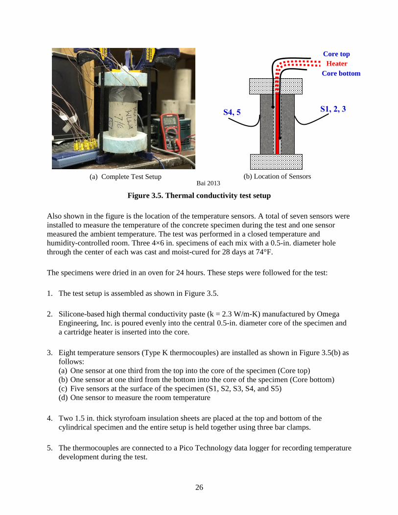
26
Bai 2013
Figure 3.5. Thermal conductivity test setup
Also shown in the figure is the location of the temperature sensors. A total of seven sensors were
installed to measure the temperature of the concrete specimen during the test and one sensor
measured the ambient temperature. The test was performed in a closed temperature and
humidity-controlled room. Three 4×6 in. specimens of each mix with a 0.5-in. diameter hole
through the center of each was cast and moist-cured for 28 days at 74°F.
The specimens were dried in an oven for 24 hours. These steps were followed for the test:
1. The test setup is assembled as shown in Figure 3.5.
2. Silicone-based high thermal conductivity paste (k = 2.3 W/m-K) manufactured by Omega
Engineering, Inc. is poured evenly into the central 0.5-in. diameter core of the specimen and
a cartridge heater is inserted into the core.
3. Eight temperature sensors (Type K thermocouples) are installed as shown in Figure 3.5(b) as
follows:
(a) One sensor at one third from the top into the core of the specimen (Core top)
(b) One sensor at one third from the bottom into the core of the specimen (Core bottom)
(c) Five sensors at the surface of the specimen (S1, S2, S3, S4, and S5)
(d) One sensor to measure the room temperature
4. Two 1.5 in. thick styrofoam insulation sheets are placed at the top and bottom of the
cylindrical specimen and the entire setup is held together using three bar clamps.
5. The thermocouples are connected to a Pico Technology data logger for recording temperature
development during the test.
Core top
S1, 2, 3
Heater
Core bottom
S4, 5
(a) Complete Test Setup (b) Location of Sensors
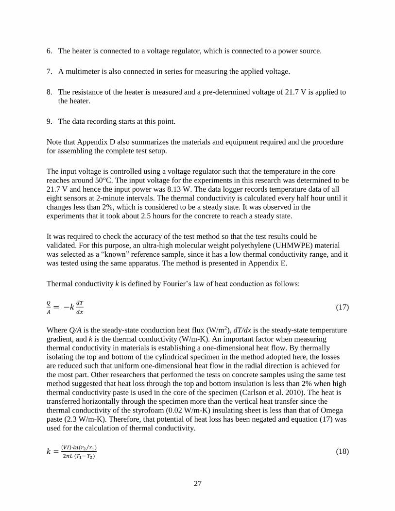
27
6. The heater is connected to a voltage regulator, which is connected to a power source.
7. A multimeter is also connected in series for measuring the applied voltage.
8. The resistance of the heater is measured and a pre-determined voltage of 21.7 V is applied to
the heater.
9. The data recording starts at this point.
Note that Appendix D also summarizes the materials and equipment required and the procedure
for assembling the complete test setup.
The input voltage is controlled using a voltage regulator such that the temperature in the core
reaches around 50°C. The input voltage for the experiments in this research was determined to be
21.7 V and hence the input power was 8.13 W. The data logger records temperature data of all
eight sensors at 2-minute intervals. The thermal conductivity is calculated every half hour until it
changes less than 2%, which is considered to be a steady state. It was observed in the
experiments that it took about 2.5 hours for the concrete to reach a steady state.
It was required to check the accuracy of the test method so that the test results could be
validated. For this purpose, an ultra-high molecular weight polyethylene (UHMWPE) material
was selected as a “known” reference sample, since it has a low thermal conductivity range, and it
was tested using the same apparatus. The method is presented in Appendix E.
Thermal conductivity k is defined by Fourier’s law of heat conduction as follows:
𝑄
𝐴= −𝑘
𝑑𝑇
𝑑𝑥 (17)
Where Q/A is the steady-state conduction heat flux (W/m2), dT/dx is the steady-state temperature
gradient, and k is the thermal conductivity (W/m-K). An important factor when measuring
thermal conductivity in materials is establishing a one-dimensional heat flow. By thermally
isolating the top and bottom of the cylindrical specimen in the method adopted here, the losses
are reduced such that uniform one-dimensional heat flow in the radial direction is achieved for
the most part. Other researchers that performed the tests on concrete samples using the same test
method suggested that heat loss through the top and bottom insulation is less than 2% when high
thermal conductivity paste is used in the core of the specimen (Carlson et al. 2010). The heat is
transferred horizontally through the specimen more than the vertical heat transfer since the
thermal conductivity of the styrofoam (0.02 W/m-K) insulating sheet is less than that of Omega
paste (2.3 W/m-K). Therefore, that potential of heat loss has been negated and equation (17) was
used for the calculation of thermal conductivity.
𝑘 =(𝑉𝐼)∙𝑙𝑛 (𝑟2 𝑟1)⁄
2𝜋𝐿 (𝑇1− 𝑇2) (18)
28
Where k is the thermal conductivity (W/m-K), VI is the power input to the heater (W), r2 is the
inner radius (m), r1 is the outer radius (m), L is the length of the specimen (m), T1 is the average
temperature in the core of the specimen (K), and T2 is the average temperature on the surface of
the specimen (K). The k value is calculated every half hour during the test, and when it changes
less than 2%, it is considered a steady state and the value at the steady state is taken as the k
value of the concrete. A minimum of three specimens was tested for each mix with two separate
runs for each specimen. The mean value of six observations was considered the thermal
conductivity of that particular mix.
Coefficient of Thermal Expansion
The coefficient of thermal expansion (CTE) is defined as the change in unit length of a material
in response to a degree of temperature change. The CTE of concrete is predominantly governed
by the type of aggregate used in the concrete mix. The CTE of all four concrete mixes in this
research were determined according to the AASHTO T 336-15 standard test method using
equipment in the Iowa State University PCC Laboratory (see Figure 3.6).
Figure 3.6. Coefficient of thermal expansion test equipment
The test method was used to determine the CTE of 4×7 in. cylindrical concrete specimens, which
were maintained in a saturated condition, by measuring the length change of specimen over a
temperature range of 10°C to 50°C. Grade 304 stainless steel with a known coefficient of
thermal expansion value was used to calibrate the test apparatus and determine the correction
factor (Cf) before the actual test was performed. Steps used in the test were as follows:
1. After 28 days of curing, 1 in. is cut off from the top of each 4×8 in. cylindrical specimen and
its length is measured to the nearest 0.004 in.
2. The specimen is placed in the support frame, making sure that the lower end of the specimen
is firmly seated against the support buttons and that the linear variable differential
transformer (LVDT) tip is seated against the upper end of the specimen.
29
3. The support frame and specimen, with the LVDT attached, is placed in the water bath, which
is filled with tap water. The height of the water is kept constant throughout the test.
4. The temperature of the water bath is set to 10°C. When the bath reaches this temperature, it is
allowed to remain at this temperature until thermal equilibrium of the specimen has been
reached, as indicated by consistent readings of the LVDT. The LVDT and temperature sensor
readings are recorded using a Campbell Scientific CR1000 data logger at one-minute
intervals.
5. The temperature of the water bath is now set to 50°C and the same thermal equilibrium
procedure is performed.
6. The temperature of the water bath is again decreased to 10°C and thermal equilibrium is
allowed to be established.
7. The CTE value is the mean of the test results of two test segments.
The CTE value of one expansion or contraction test segment is calculated as follows:
CTE =∆La/∆Lo
∆T (19)
∆La = ∆Lm + ∆Lf (20)
∆Lf = Cf × Lo × ∆T (21)
Where ∆La is the actual length change of specimen during the temperature change (mm), Lo is
the measured length of the specimen at room temperature (mm), ∆T is the measured temperature
change, (°C), ∆Lm is the measured length change of specimen during temperature change (mm),
∆Lf is length change of the measuring apparatus during temperature change (mm), and Cf is the
correction factor (microstrain/°C).
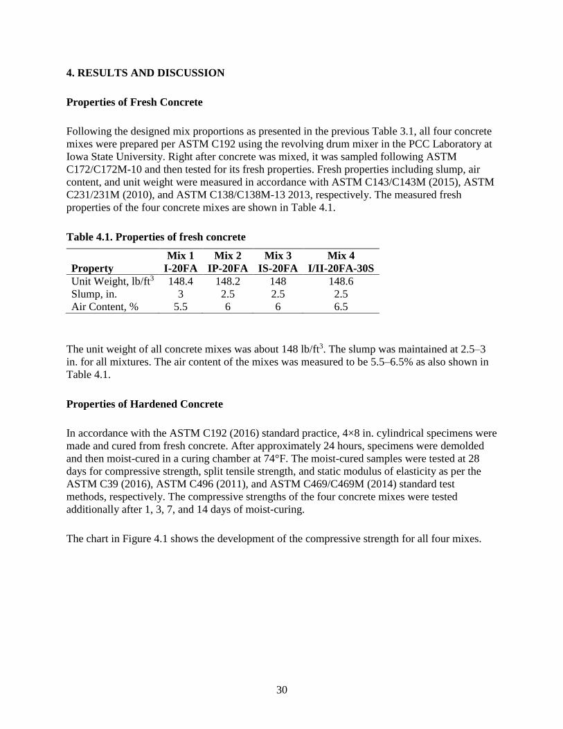
30
4. RESULTS AND DISCUSSION
Properties of Fresh Concrete
Following the designed mix proportions as presented in the previous Table 3.1, all four concrete
mixes were prepared per ASTM C192 using the revolving drum mixer in the PCC Laboratory at
Iowa State University. Right after concrete was mixed, it was sampled following ASTM
C172/C172M-10 and then tested for its fresh properties. Fresh properties including slump, air
content, and unit weight were measured in accordance with ASTM C143/C143M (2015), ASTM
C231/231M (2010), and ASTM C138/C138M-13 2013, respectively. The measured fresh
properties of the four concrete mixes are shown in Table 4.1.
Table 4.1. Properties of fresh concrete
Property
Mix 1
I-20FA
Mix 2
IP-20FA
Mix 3
IS-20FA
Mix 4
I/II-20FA-30S
Unit Weight, lb/ft3 148.4 148.2 148 148.6
Slump, in. 3 2.5 2.5 2.5
Air Content, % 5.5 6 6 6.5
The unit weight of all concrete mixes was about 148 lb/ft3. The slump was maintained at 2.5–3
in. for all mixtures. The air content of the mixes was measured to be 5.5–6.5% as also shown in
Table 4.1.
Properties of Hardened Concrete
In accordance with the ASTM C192 (2016) standard practice, 4×8 in. cylindrical specimens were
made and cured from fresh concrete. After approximately 24 hours, specimens were demolded
and then moist-cured in a curing chamber at 74°F. The moist-cured samples were tested at 28
days for compressive strength, split tensile strength, and static modulus of elasticity as per the
ASTM C39 (2016), ASTM C496 (2011), and ASTM C469/C469M (2014) standard test
methods, respectively. The compressive strengths of the four concrete mixes were tested
additionally after 1, 3, 7, and 14 days of moist-curing.
The chart in Figure 4.1 shows the development of the compressive strength for all four mixes.
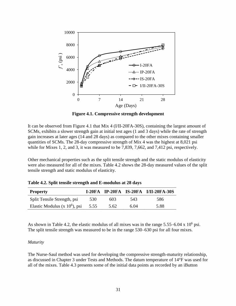
31
Figure 4.1. Compressive strength development
It can be observed from Figure 4.1 that Mix 4 (I/II-20FA-30S), containing the largest amount of
SCMs, exhibits a slower strength gain at initial test ages (1 and 3 days) while the rate of strength
gain increases at later ages (14 and 28 days) as compared to the other mixes containing smaller
quantities of SCMs. The 28-day compressive strength of Mix 4 was the highest at 8,021 psi
while for Mixes 1, 2, and 3, it was measured to be 7,839, 7,662, and 7,412 psi, respectively.
Other mechanical properties such as the split tensile strength and the static modulus of elasticity
were also measured for all of the mixes. Table 4.2 shows the 28-day measured values of the split
tensile strength and static modulus of elasticity.
Table 4.2. Split tensile strength and E-modulus at 28 days
Property I-20FA IP-20FA IS-20FA I/II-20FA-30S
Split Tensile Strength, psi 530 603 543 586
Elastic Modulus (x 106), psi 5.55 5.62 6.04 5.88
As shown in Table 4.2, the elastic modulus of all mixes was in the range 5.55–6.04 x 10⁶ psi.
The split tensile strength was measured to be in the range 530–630 psi for all four mixes.
Maturity
The Nurse-Saul method was used for developing the compressive strength-maturity relationship,
as discussed in Chapter 3 under Tests and Methods. The datum temperature of 14°F was used for
all of the mixes. Table 4.3 presents some of the initial data points as recorded by an iButton
0
2000
4000
6000
8000
10000
0 7 14 21 28
’ c
(psi
)
Age (Days)
I-20FA
IP-20FA
IS-20FA
I/II-20FA-30S
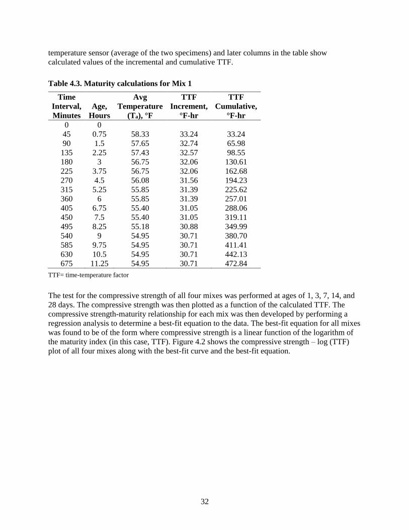
32
temperature sensor (average of the two specimens) and later columns in the table show
calculated values of the incremental and cumulative TTF.
Table 4.3. Maturity calculations for Mix 1
Time
Interval,
Minutes
Age,
Hours
Avg
Temperature
(Ta), °F
TTF
Increment,
°F-hr
TTF
Cumulative,
°F-hr
0 0
45 0.75 58.33 33.24 33.24
90 1.5 57.65 32.74 65.98
135 2.25 57.43 32.57 98.55
180 3 56.75 32.06 130.61
225 3.75 56.75 32.06 162.68
270 4.5 56.08 31.56 194.23
315 5.25 55.85 31.39 225.62
360 6 55.85 31.39 257.01
405 6.75 55.40 31.05 288.06
450 7.5 55.40 31.05 319.11
495 8.25 55.18 30.88 349.99
540 9 54.95 30.71 380.70
585 9.75 54.95 30.71 411.41
630 10.5 54.95 30.71 442.13
675 11.25 54.95 30.71 472.84
TTF= time-temperature factor
The test for the compressive strength of all four mixes was performed at ages of 1, 3, 7, 14, and
28 days. The compressive strength was then plotted as a function of the calculated TTF. The
compressive strength-maturity relationship for each mix was then developed by performing a
regression analysis to determine a best-fit equation to the data. The best-fit equation for all mixes
was found to be of the form where compressive strength is a linear function of the logarithm of
the maturity index (in this case, TTF). Figure 4.2 shows the compressive strength – log (TTF)
plot of all four mixes along with the best-fit curve and the best-fit equation.
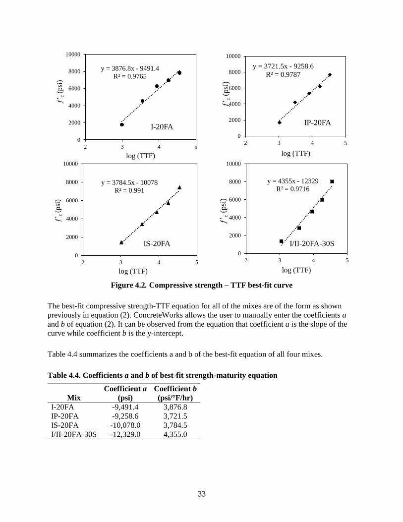
33
Figure 4.2. Compressive strength – TTF best-fit curve
The best-fit compressive strength-TTF equation for all of the mixes are of the form as shown
previously in equation (2). ConcreteWorks allows the user to manually enter the coefficients a
and b of equation (2). It can be observed from the equation that coefficient a is the slope of the
curve while coefficient b is the y-intercept.
Table 4.4 summarizes the coefficients a and b of the best-fit equation of all four mixes.
Table 4.4. Coefficients a and b of best-fit strength-maturity equation
Mix
Coefficient a
(psi)
Coefficient b
(psi/°F/hr)
I-20FA -9,491.4 3,876.8
IP-20FA -9,258.6 3,721.5
IS-20FA -10,078.0 3,784.5
I/II-20FA-30S -12,329.0 4,355.0
y = 3876.8x - 9491.4
R² = 0.9765
0
2000
4000
6000
8000
10000
2 3 4 5
’ c
(psi
)
log (TTF)
I-20FA
y = 3721.5x - 9258.6
R² = 0.9787
0
2000
4000
6000
8000
10000
2 3 4 5
’ c
(psi
)
log (TTF)
IP-20FA
y = 3784.5x - 10078
R² = 0.991
0
2000
4000
6000
8000
10000
2 3 4 5
’ c
(psi
)
log (TTF)
IS-20FA
y = 4355x - 12329
R² = 0.9716
0
2000
4000
6000
8000
10000
2 3 4 5
’ c
(psi
)
log (TTF)
I/II-20FA-30S
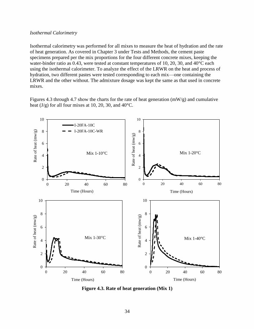
34
Isothermal Calorimetry
Isothermal calorimetry was performed for all mixes to measure the heat of hydration and the rate
of heat generation. As covered in Chapter 3 under Tests and Methods, the cement paste
specimens prepared per the mix proportions for the four different concrete mixes, keeping the
water-binder ratio as 0.43, were tested at constant temperatures of 10, 20, 30, and 40°C each
using the isothermal calorimeter. To analyze the effect of the LRWR on the heat and process of
hydration, two different pastes were tested corresponding to each mix—one containing the
LRWR and the other without. The admixture dosage was kept the same as that used in concrete
mixes.
Figures 4.3 through 4.7 show the charts for the rate of heat generation (mW/g) and cumulative
heat (J/g) for all four mixes at 10, 20, 30, and 40°C.
Figure 4.3. Rate of heat generation (Mix 1)
0
2
4
6
8
10
0 20 40 60 80
Rat
e o
f hea
t (m
w/g
)
Time (Hours)
Mix 1-10°C
I-20FA-10C
I-20FA-10C-WR
0
2
4
6
8
10
0 20 40 60 80
Rat
e o
f hea
t (m
w/g
)
Time (Hours)
Mix 1-20°C
0
2
4
6
8
10
0 20 40 60 80
Rat
e o
f hea
t (m
w/g
)
Time (Hours)
Mix 1-30°C
0
2
4
6
8
10
0 20 40 60 80
Rat
e o
f hea
t (m
w/g
)
Time (Hours)
Mix 1-40°C
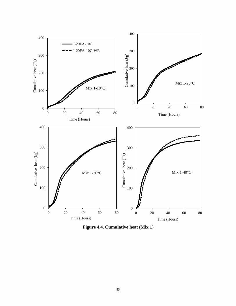
35
Figure 4.4. Cumulative heat (Mix 1)
0
100
200
300
400
0 20 40 60 80
Cum
ula
tive
hea
t (J
/g)
Time (Hours)
Mix 1-10°C
I-20FA-10C
I-20FA-10C-WR
0
100
200
300
400
0 20 40 60 80
Cum
ula
tive
hea
t (J
/g)
Time (Hours)
Mix 1-20°C
0
100
200
300
400
0 20 40 60 80
Cum
ula
tive
hea
t (J
/g)
Time (Hours)
Mix 1-30°C
0
100
200
300
400
0 20 40 60 80
Cum
ula
tive
hea
t (J
/g)
Time (Hours)
Mix 1-40°C
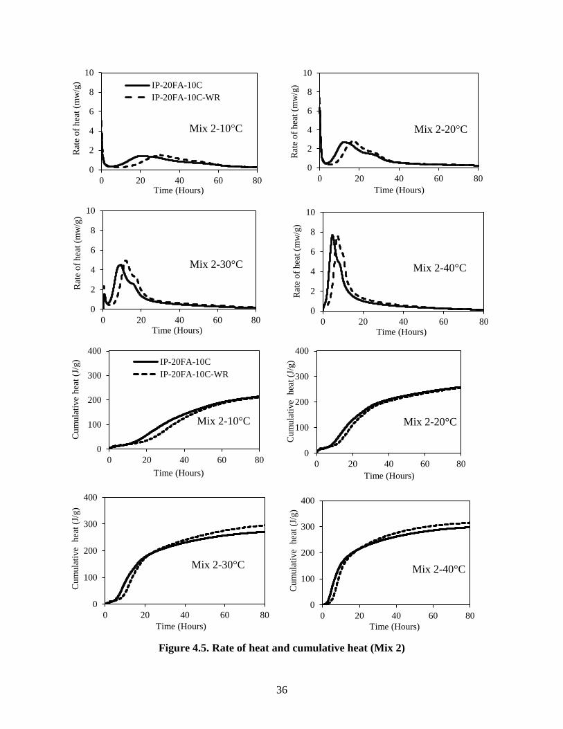
36
Figure 4.5. Rate of heat and cumulative heat (Mix 2)
0
2
4
6
8
10
0 20 40 60 80
Rat
e o
f hea
t (m
w/g
)
Time (Hours)
Mix 2-10°C
IP-20FA-10C
IP-20FA-10C-WR
0
2
4
6
8
10
0 20 40 60 80
Rat
e o
f hea
t (m
w/g
)
Time (Hours)
Mix 2-30°C
0
100
200
300
400
0 20 40 60 80
Cum
ula
tive
hea
t (J
/g)
Time (Hours)
Mix 2-10°C
IP-20FA-10C
IP-20FA-10C-WR
0
100
200
300
400
0 20 40 60 80
Cum
ula
tive
hea
t (J
/g)
Time (Hours)
Mix 2-20°C
0
100
200
300
400
0 20 40 60 80
Cum
ula
tive
hea
t (J
/g)
Time (Hours)
Mix 2-30°C
0
100
200
300
400
0 20 40 60 80
Cum
ula
tive
hea
t (J
/g)
Time (Hours)
Mix 2-40°C
0
2
4
6
8
10
0 20 40 60 80
Rat
e o
f hea
t (m
w/g
)
Time (Hours)
Mix 2-20°C
0
2
4
6
8
10
0 20 40 60 80
Rat
e o
f hea
t (m
w/g
)
Time (Hours)
Mix 2-40°C
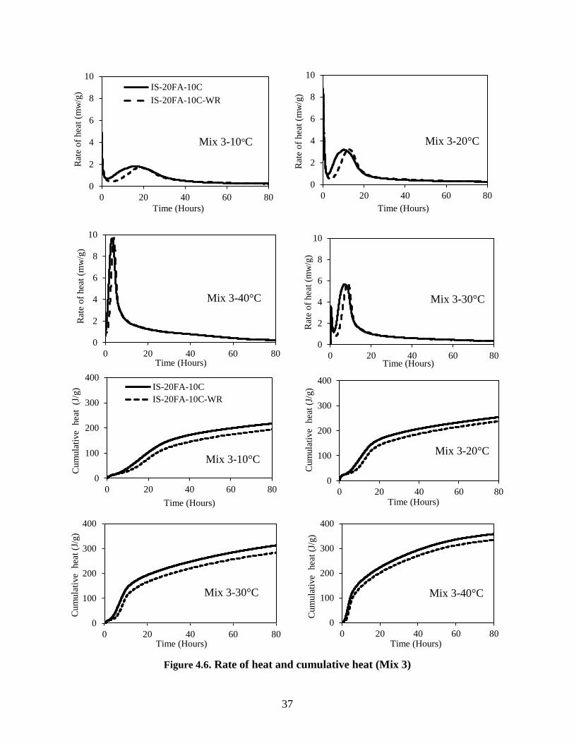
37
Figure 4.6. Rate of heat and cumulative heat (Mix 3)
0
2
4
6
8
10
0 20 40 60 80
Rat
e o
f hea
t (m
w/g
)
Time (Hours)
Mix 3-20°C
0
100
200
300
400
0 20 40 60 80
Cum
ula
tive
hea
t (
J/g)
Time (Hours)
Mix 3-10°C
IS-20FA-10C
IS-20FA-10C-WR
0
100
200
300
400
0 20 40 60 80
Cum
ula
tive
hea
t (J
/g)
Time (Hours)
Mix 3-30°C
0
100
200
300
400
0 20 40 60 80
Cum
ula
tive
hea
t (J
/g)
Time (Hours)
Mix 3-40°C
0
2
4
6
8
10
0 20 40 60 80
Rat
e o
f hea
t (m
w/g
)
Time (Hours)
Mix 3-40°C
0
2
4
6
8
10
0 20 40 60 80
Rat
e o
f hea
t (m
w/g
)
Time (Hours)
Mix 3-10°C
IS-20FA-10C
IS-20FA-10C-WR
0
2
4
6
8
10
0 20 40 60 80
Rat
e o
f hea
t (m
w/g
)
Time (Hours)
Mix 3-30°C
0
100
200
300
400
0 20 40 60 80
Cum
ula
tive
hea
t (J
/g)
Time (Hours)
Mix 3-20°C
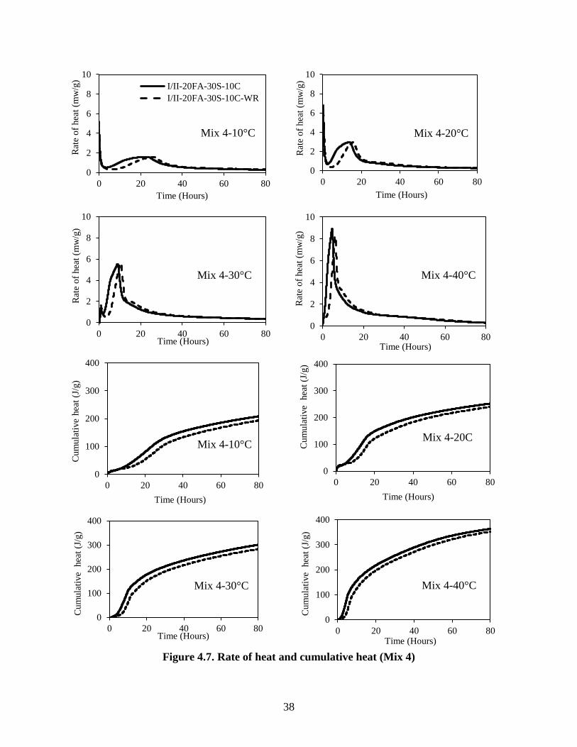
38
Figure 4.7. Rate of heat and cumulative heat (Mix 4)
0
2
4
6
8
10
0 20 40 60 80
Rat
e o
f hea
t (m
w/g
)
Time (Hours)
Mix 4-10°C
I/II-20FA-30S-10C
I/II-20FA-30S-10C-WR
0
2
4
6
8
10
0 20 40 60 80
Rat
e o
f hea
t (m
w/g
)
Time (Hours)
Mix 4-30°C
0
100
200
300
400
0 20 40 60 80
Cum
ula
tive
hea
t (J
/g)
Time (Hours)
Mix 4-10°C
0
100
200
300
400
0 20 40 60 80
Cum
ula
tive
hea
t (J
/g)
Time (Hours)
Mix 4-30°C
0
2
4
6
8
10
0 20 40 60 80
Rat
e o
f hea
t (m
w/g
)
Time (Hours)
Mix 4-40°C
0
100
200
300
400
0 20 40 60 80
Cum
ula
tive
hea
t (J
/g)
Time (Hours)
Mix 4-20C
0
2
4
6
8
10
0 20 40 60 80
Rat
e o
f hea
t (m
w/g
)
Time (Hours)
Mix 4-20°C
0
100
200
300
400
0 20 40 60 80
Cum
ula
tive
hea
t (J
/g)
Time (Hours)
Mix 4-40°C
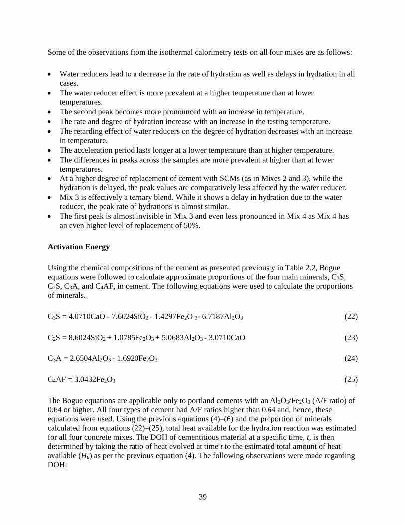
39
Some of the observations from the isothermal calorimetry tests on all four mixes are as follows:
Water reducers lead to a decrease in the rate of hydration as well as delays in hydration in all
cases.
The water reducer effect is more prevalent at a higher temperature than at lower
temperatures.
The second peak becomes more pronounced with an increase in temperature.
The rate and degree of hydration increase with an increase in the testing temperature.
The retarding effect of water reducers on the degree of hydration decreases with an increase
in temperature.
The acceleration period lasts longer at a lower temperature than at higher temperature.
The differences in peaks across the samples are more prevalent at higher than at lower
temperatures.
At a higher degree of replacement of cement with SCMs (as in Mixes 2 and 3), while the
hydration is delayed, the peak values are comparatively less affected by the water reducer.
Mix 3 is effectively a ternary blend. While it shows a delay in hydration due to the water
reducer, the peak rate of hydrations is almost similar.
The first peak is almost invisible in Mix 3 and even less pronounced in Mix 4 as Mix 4 has
an even higher level of replacement of 50%.
Activation Energy
Using the chemical compositions of the cement as presented previously in Table 2.2, Bogue
equations were followed to calculate approximate proportions of the four main minerals, C3S,
C2S, C3A, and C4AF, in cement. The following equations were used to calculate the proportions
of minerals.
C3S = 4.0710CaO - 7.6024SiO2 - 1.4297Fe2O 3- 6.7187Al2O3 (22)
C2S = 8.6024SiO2 + 1.0785Fe2O3 + 5.0683Al2O3 - 3.0710CaO (23)
C3A = 2.6504Al2O3 - 1.6920Fe2O3 (24)
C4AF = 3.0432Fe2O3 (25)
The Bogue equations are applicable only to portland cements with an Al2O3/Fe2O3 (A/F ratio) of
0.64 or higher. All four types of cement had A/F ratios higher than 0.64 and, hence, these
equations were used. Using the previous equations (4)–(6) and the proportion of minerals
calculated from equations (22)–(25), total heat available for the hydration reaction was estimated
for all four concrete mixes. The DOH of cementitious material at a specific time, t, is then
determined by taking the ratio of heat evolved at time t to the estimated total amount of heat
available (Hu) as per the previous equation (4). The following observations were made regarding
DOH:
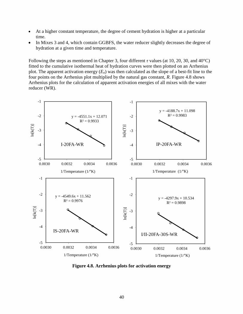
40
At a higher constant temperature, the degree of cement hydration is higher at a particular
time.
In Mixes 3 and 4, which contain GGBFS, the water reducer slightly decreases the degree of
hydration at a given time and temperature.
Following the steps as mentioned in Chapter 3, four different τ values (at 10, 20, 30, and 40°C)
fitted to the cumulative isothermal heat of hydration curves were then plotted on an Arrhenius
plot. The apparent activation energy (Ea) was then calculated as the slope of a best-fit line to the
four points on the Arrhenius plot multiplied by the natural gas constant, R. Figure 4.8 shows
Arrhenius plots for the calculation of apparent activation energies of all mixes with the water
reducer (WR).
Figure 4.8. Arrhenius plots for activation energy
y = -4551.1x + 12.071
R² = 0.9933
-5
-4
-3
-2
-1
0.0030 0.0032 0.0034 0.0036
ln[k
(T)]
1/Temperature (1/°K)
I-20FA-WR
y = -4188.7x + 11.098
R² = 0.9983
-5
-4
-3
-2
-1
0.0030 0.0032 0.0034 0.0036
ln[k
(T)]
1/Temperature (1/°K)
IP-20FA-WR
y = -4549.6x + 11.562
R² = 0.9976
-5
-4
-3
-2
-1
0.0030 0.0032 0.0034 0.0036
ln[k
(T)]
1/Temperature (1/°K)
IS-20FA-WR
y = -4297.9x + 10.534
R² = 0.9898
-5
-4
-3
-2
-1
0.0030 0.0032 0.0034 0.0036
ln[k
(T)]
1/Temperature (1/°K)
I/II-20FA-30S-WR
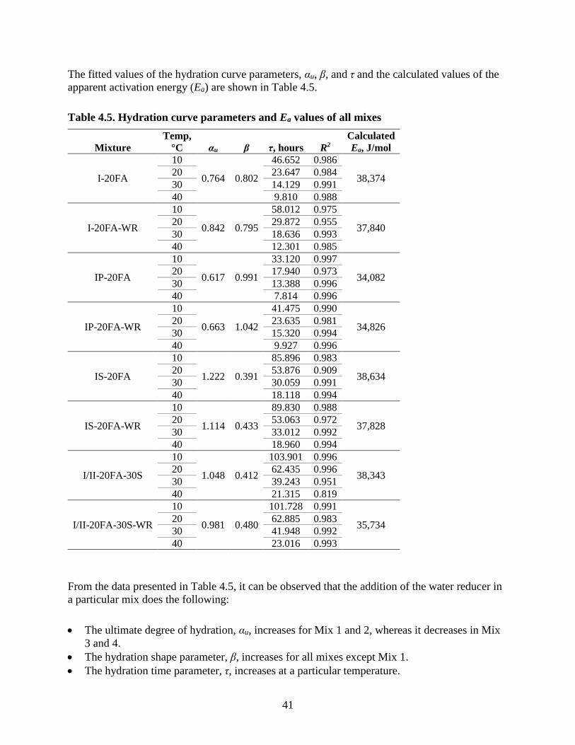
41
The fitted values of the hydration curve parameters, αu, β, and τ and the calculated values of the
apparent activation energy (Ea) are shown in Table 4.5.
Table 4.5. Hydration curve parameters and Ea values of all mixes
Mixture
Temp,
°C αu β τ, hours R2
Calculated
Ea, J/mol
I-20FA
10
0.764 0.802
46.652 0.986
38,374 20 23.647 0.984
30 14.129 0.991
40 9.810 0.988
I-20FA-WR
10
0.842 0.795
58.012 0.975
37,840 20 29.872 0.955
30 18.636 0.993
40 12.301 0.985
IP-20FA
10
0.617 0.991
33.120 0.997
34,082 20 17.940 0.973
30 13.388 0.996
40 7.814 0.996
IP-20FA-WR
10
0.663 1.042
41.475 0.990
34,826 20 23.635 0.981
30 15.320 0.994
40 9.927 0.996
IS-20FA
10
1.222 0.391
85.896 0.983
38,634 20 53.876 0.909
30 30.059 0.991
40 18.118 0.994
IS-20FA-WR
10
1.114 0.433
89.830 0.988
37,828 20 53.063 0.972
30 33.012 0.992
40 18.960 0.994
I/II-20FA-30S
10
1.048 0.412
103.901 0.996
38,343 20 62.435 0.996
30 39.243 0.951
40 21.315 0.819
I/II-20FA-30S-WR
10
0.981 0.480
101.728 0.991
35,734 20 62.885 0.983
30 41.948 0.992
40 23.016 0.993
From the data presented in Table 4.5, it can be observed that the addition of the water reducer in
a particular mix does the following:
The ultimate degree of hydration, αu, increases for Mix 1 and 2, whereas it decreases in Mix
3 and 4.
The hydration shape parameter, β, increases for all mixes except Mix 1.
The hydration time parameter, τ, increases at a particular temperature.
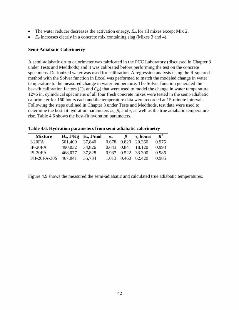
42
The water reducer decreases the activation energy, Ea, for all mixes except Mix 2.
Ea increases clearly in a concrete mix containing slag (Mixes 3 and 4).
Semi-Adiabatic Calorimetry
A semi-adiabatic drum calorimeter was fabricated in the PCC Laboratory (discussed in Chapter 3
under Tests and Medthods) and it was calibrated before performing the test on the concrete
specimens. De-ionized water was used for calibration. A regression analysis using the R-squared
method with the Solver function in Excel was performed to match the modeled change in water
temperature to the measured change in water temperature. The Solver function generated the
best-fit calibration factors (Cf1 and Cf2) that were used to model the change in water temperature.
12×6 in. cylindrical specimens of all four fresh concrete mixes were tested in the semi-adiabatic
calorimeter for 160 hours each and the temperature data were recorded at 15-minute intervals.
Following the steps outlined in Chapter 3 under Tests and Medthods, test data were used to
determine the best-fit hydration parameters αu, β, and τ, as well as the true adiabatic temperature
rise. Table 4.6 shows the best-fit hydration parameters.
Table 4.6. Hydration parameters from semi-adiabatic calorimetry
Mixture Hu, J/Kg Ea, J/mol αu β τ, hours R2
I-20FA 501,400 37,840 0.678 0.820 20.360 0.975
IP-20FA 490,032 34,826 0.643 0.841 18.120 0.993
IS-20FA 468,077 37,828 0.937 0.522 33.300 0.986
I/II-20FA-30S 467,041 35,734 1.013 0.460 62.420 0.985
Figure 4.9 shows the measured the semi-adiabatic and calculated true adiabatic temperatures.
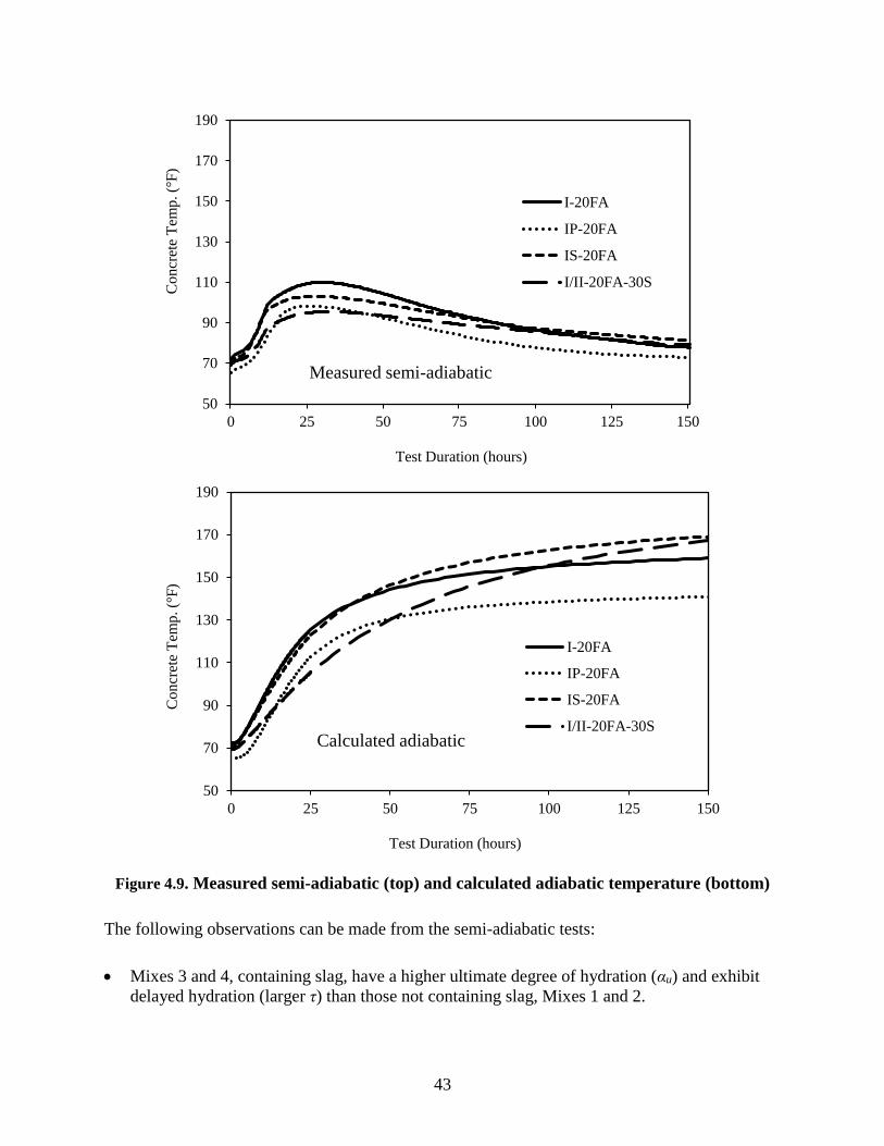
43
Figure 4.9. Measured semi-adiabatic (top) and calculated adiabatic temperature (bottom)
The following observations can be made from the semi-adiabatic tests:
Mixes 3 and 4, containing slag, have a higher ultimate degree of hydration (αu) and exhibit
delayed hydration (larger τ) than those not containing slag, Mixes 1 and 2.
50
70
90
110
130
150
170
190
0 25 50 75 100 125 150
Co
ncr
ete
Tem
p. (°
F)
Test Duration (hours)
Measured semi-adiabatic
I-20FA
IP-20FA
IS-20FA
I/II-20FA-30S
50
70
90
110
130
150
170
190
0 25 50 75 100 125 150
Concr
ete
Tem
p. (°
F)
Test Duration (hours)
Calculated adiabatic
I-20FA
IP-20FA
IS-20FA
I/II-20FA-30S
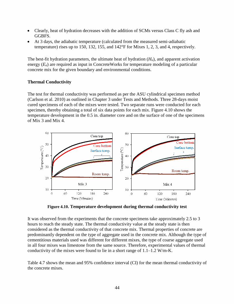
44
Clearly, heat of hydration decreases with the addition of SCMs versus Class C fly ash and
GGBFS.
At 3 days, the adiabatic temperature (calculated from the measured semi-adiabatic
temperature) rises up to 150, 132, 155, and 142°F for Mixes 1, 2, 3, and 4, respectively.
The best-fit hydration parameters, the ultimate heat of hydration (Hu), and apparent activation
energy (Ea) are required as input in ConcreteWorks for temperature modeling of a particular
concrete mix for the given boundary and environmental conditions.
Thermal Conductivity
The test for thermal conductivity was performed as per the ASU cylindrical specimen method
(Carlson et al. 2010) as outlined in Chapter 3 under Tests and Methods. Three 28-days moist
cured specimens of each of the mixes were tested. Two separate runs were conducted for each
specimen, thereby obtaining a total of six data points for each mix. Figure 4.10 shows the
temperature development in the 0.5 in. diameter core and on the surface of one of the specimens
of Mix 3 and Mix 4.
Figure 4.10. Temperature development during thermal conductivity test
It was observed from the experiments that the concrete specimens take approximately 2.5 to 3
hours to reach the steady state. The thermal conductivity value at the steady state is then
considered as the thermal conductivity of that concrete mix. Thermal properties of concrete are
predominantly dependent on the type of aggregate used in the concrete mix. Although the type of
cementitious materials used was different for different mixes, the type of coarse aggregate used
in all four mixes was limestone from the same source. Therefore, experimental values of thermal
conductivity of the mixes were found to lie in a short range of 1.1–1.2 W/m-K.
Table 4.7 shows the mean and 95% confidence interval (CI) for the mean thermal conductivity of
the concrete mixes.
45
Table 4.7. 95% confidence interval for mean thermal conductivity
Mix Mean k (W/m-K) 95% CI for Mean k (W/m-K)
I-20FA 1.20 (1.15–1.26)
IP-20FA 1.17 (1.15–1.18)
IS-20FA 1.12 (1.09–1.14)
I/II-20FA-30S 1.10 (1.06–1.14)
The confidence interval signifies that if the test is performed several times, it can be believed that
95% of the thermal conductivity values would lie in this interval. The default value of thermal
conductivity in ConcreteWorks is 2.6 W/m-K.
Coefficient of Thermal Expansion
The coefficient of thermal expansion was determined using the AASHTO T 336-15 test method
(discussed in Chapter 3 under Tests and Methods). Two 28-day moist-cured specimens of each
of the mixes were used to perform the CTE test. Table 4.8 shows the measured CTE values of
the mixes.
Table 4.8. CTE values of concrete mixes
Property Mix 1 Mix 2 Mix 3 Mix 4
CTE (microstrain/°C) 8.03 8.16 9.08 7.19
As discussed in the last section, the thermal properties of concrete are predominantly dependent
on the type of aggregate used in the concrete mix. In this research, limestone was used as coarse
aggregate for all four mixes and, hence, the CTE value of all mixes were measured to be in a
small range of 7.19–9.08 microstrain/°C.

46
5. FIELD INVESTIGATION
As part of Task 4, the construction of Pier 4 of I-35 NB to the US 30 WB (Ramp H) bridge in
Ames, Iowa was analyzed and the process was documented. Figure 5.1 shows the location
designated as DESIGN NO. 616.
Iowa DOT Office of Bridges and Structures 2016
Figure 5.1. Location of the I-35 to US 30 Bridge
The I-35 NB to US 30 WB (Ramp H) bridge is a seven-span continuous welded girder bridge
constructed on six piers with a total length of 1,690 ft and a width of 36 ft extending from Station
8517+07 to Station 8533+97.
All of the piers have a rectangular cross section except one, the footing of Pier 3, which has a
cross section of a rectangle cut on the two opposite corners. The footing of Pier 4 (Footing #4)
was selected as the focus of the field investigation in this project as it is the largest of all of the
footings; the stem and column were not investigated. Figure 5.2 shows the location of all six
bridge piers.
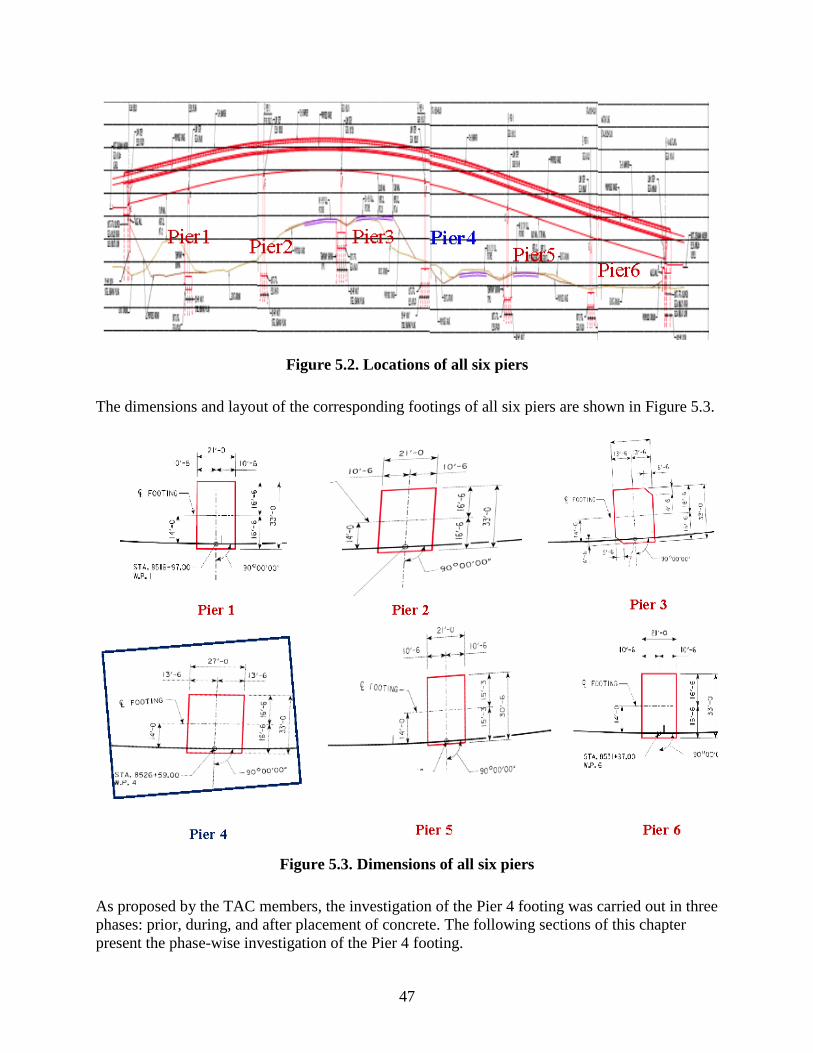
47
Figure 5.2. Locations of all six piers
The dimensions and layout of the corresponding footings of all six piers are shown in Figure 5.3.
Figure 5.3. Dimensions of all six piers
As proposed by the TAC members, the investigation of the Pier 4 footing was carried out in three
phases: prior, during, and after placement of concrete. The following sections of this chapter
present the phase-wise investigation of the Pier 4 footing.
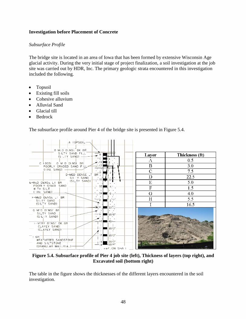
48
Investigation before Placement of Concrete
Subsurface Profile
The bridge site is located in an area of Iowa that has been formed by extensive Wisconsin Age
glacial activity. During the very initial stage of project finalization, a soil investigation at the job
site was carried out by HDR, Inc. The primary geologic strata encountered in this investigation
included the following.
Topsoil
Existing fill soils
Cohesive alluvium
Alluvial Sand
Glacial till
Bedrock
The subsurface profile around Pier 4 of the bridge site is presented in Figure 5.4.
Figure 5.4. Subsurface profile of Pier 4 job site (left), Thickness of layers (top right), and
Excavated soil (bottom right)
The table in the figure shows the thicknesses of the different layers encountered in the soil
investigation.
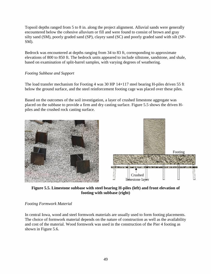
49
Topsoil depths ranged from 5 to 8 in. along the project alignment. Alluvial sands were generally
encountered below the cohesive alluvium or fill and were found to consist of brown and gray
silty sand (SM), poorly graded sand (SP), clayey sand (SC) and poorly graded sand with silt (SP-
SM).
Bedrock was encountered at depths ranging from 34 to 83 ft, corresponding to approximate
elevations of 800 to 850 ft. The bedrock units appeared to include siltstone, sandstone, and shale,
based on examination of split-barrel samples, with varying degrees of weathering.
Footing Subbase and Support
The load transfer mechanism for Footing 4 was 30 HP 14×117 steel bearing H-piles driven 55 ft
below the ground surface, and the steel reinforcement footing cage was placed over these piles.
Based on the outcomes of the soil investigation, a layer of crushed limestone aggregate was
placed on the subbase to provide a firm and dry casting surface. Figure 5.5 shows the driven H-
piles and the crushed rock casting surface.
Figure 5.5. Limestone subbase with steel bearing H-piles (left) and front elevation of
footing with subbase (right)
Footing Formwork Material
In central Iowa, wood and steel formwork materials are usually used to form footing placements.
The choice of formwork material depends on the nature of construction as well as the availability
and cost of the material. Wood formwork was used in the construction of the Pier 4 footing as
shown in Figure 5.6.
Crushed
limestone layer
Footing
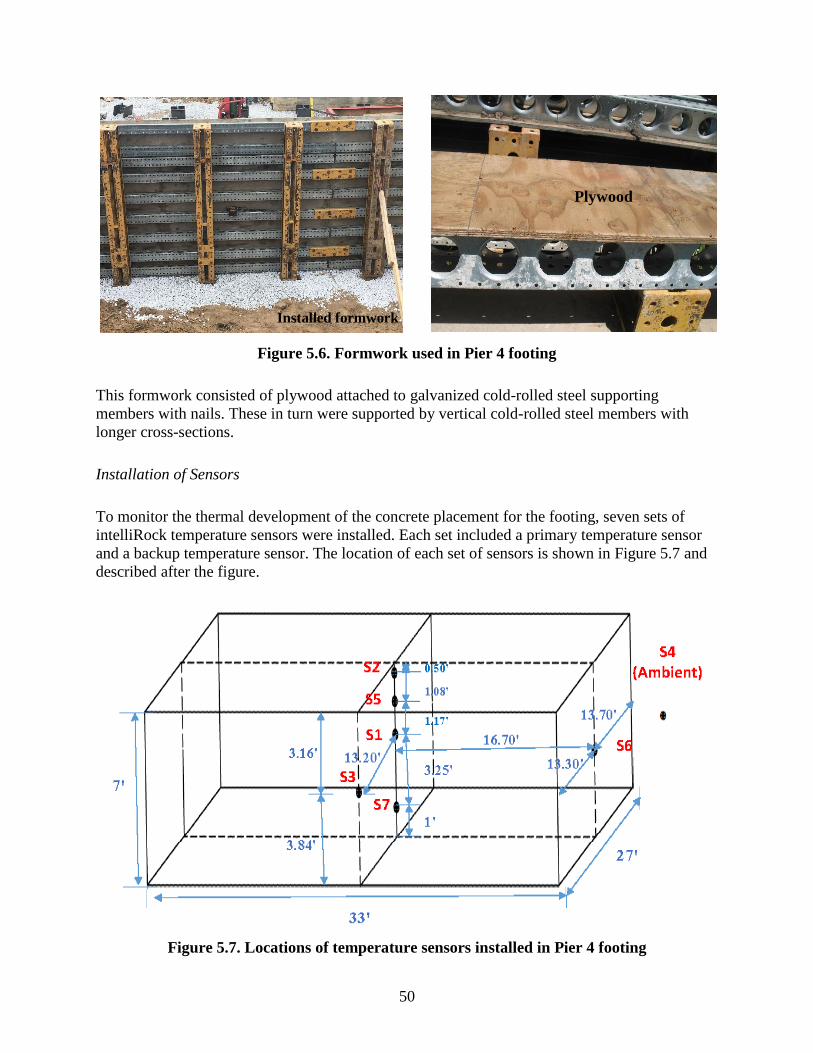
50
Figure 5.6. Formwork used in Pier 4 footing
This formwork consisted of plywood attached to galvanized cold-rolled steel supporting
members with nails. These in turn were supported by vertical cold-rolled steel members with
longer cross-sections.
Installation of Sensors
To monitor the thermal development of the concrete placement for the footing, seven sets of
intelliRock temperature sensors were installed. Each set included a primary temperature sensor
and a backup temperature sensor. The location of each set of sensors is shown in Figure 5.7 and
described after the figure.
Figure 5.7. Locations of temperature sensors installed in Pier 4 footing
Installed formwork
Plywood
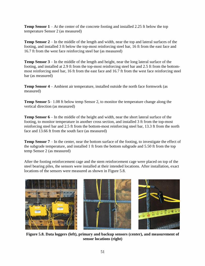
51
Temp Sensor 1 – At the center of the concrete footing and installed 2.25 ft below the top
temperature Sensor 2 (as measured)
Temp Sensor 2 – In the middle of the length and width, near the top and lateral surfaces of the
footing, and installed 3 ft below the top-most reinforcing steel bar, 16 ft from the east face and
16.7 ft from the west face reinforcing steel bar (as measured)
Temp Sensor 3 – In the middle of the length and height, near the long lateral surface of the
footing, and installed at 2.9 ft from the top-most reinforcing steel bar and 2.5 ft from the bottom-
most reinforcing steel bar, 16 ft from the east face and 16.7 ft from the west face reinforcing steel
bar (as measured)
Temp Sensor 4 – Ambient air temperature, installed outside the north face formwork (as
measured)
Temp Sensor 5– 1.08 ft below temp Sensor 2, to monitor the temperature change along the
vertical direction (as measured)
Temp Sensor 6 – In the middle of the height and width, near the short lateral surface of the
footing, to monitor temperature in another cross section, and installed 3 ft from the top-most
reinforcing steel bar and 2.5 ft from the bottom-most reinforcing steel bar, 13.3 ft from the north
face and 13.66 ft from the south face (as measured)
Temp Sensor 7 – In the center, near the bottom surface of the footing, to investigate the effect of
the subgrade temperature, and installed 1 ft from the bottom subgrade and 5.50 ft from the top
temp Sensor 2 (as measured)
After the footing reinforcement cage and the stem reinforcement cage were placed on top of the
steel bearing piles, the sensors were installed at their intended locations. After installation, exact
locations of the sensors were measured as shown in Figure 5.8.
Figure 5.8. Data loggers (left), primary and backup sensors (center), and measurement of
sensor locations (right)
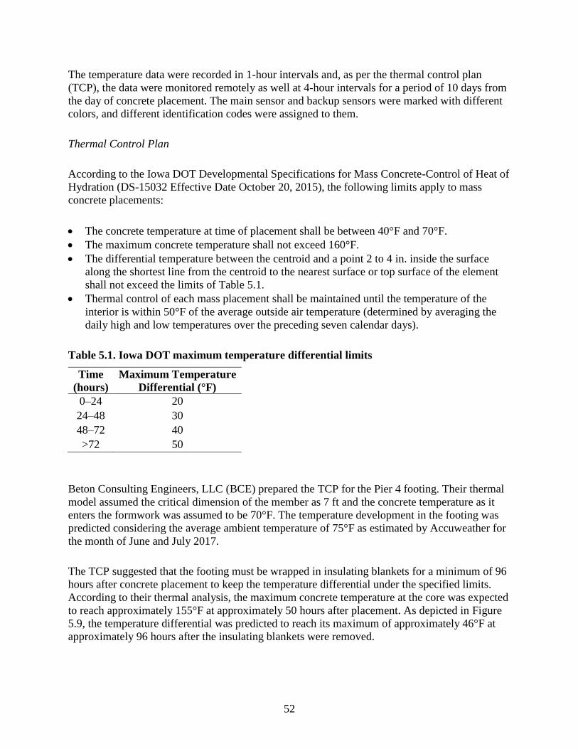
52
The temperature data were recorded in 1-hour intervals and, as per the thermal control plan
(TCP), the data were monitored remotely as well at 4-hour intervals for a period of 10 days from
the day of concrete placement. The main sensor and backup sensors were marked with different
colors, and different identification codes were assigned to them.
Thermal Control Plan
According to the Iowa DOT Developmental Specifications for Mass Concrete-Control of Heat of
Hydration (DS-15032 Effective Date October 20, 2015), the following limits apply to mass
concrete placements:
The concrete temperature at time of placement shall be between 40°F and 70°F.
The maximum concrete temperature shall not exceed 160°F.
The differential temperature between the centroid and a point 2 to 4 in. inside the surface
along the shortest line from the centroid to the nearest surface or top surface of the element
shall not exceed the limits of Table 5.1.
Thermal control of each mass placement shall be maintained until the temperature of the
interior is within 50°F of the average outside air temperature (determined by averaging the
daily high and low temperatures over the preceding seven calendar days).
Table 5.1. Iowa DOT maximum temperature differential limits
Time
(hours)
Maximum Temperature
Differential (°F)
0–24 20
24–48 30
48–72 40
>72 50
Beton Consulting Engineers, LLC (BCE) prepared the TCP for the Pier 4 footing. Their thermal
model assumed the critical dimension of the member as 7 ft and the concrete temperature as it
enters the formwork was assumed to be 70°F. The temperature development in the footing was
predicted considering the average ambient temperature of 75°F as estimated by Accuweather for
the month of June and July 2017.
The TCP suggested that the footing must be wrapped in insulating blankets for a minimum of 96
hours after concrete placement to keep the temperature differential under the specified limits.
According to their thermal analysis, the maximum concrete temperature at the core was expected
to reach approximately 155°F at approximately 50 hours after placement. As depicted in Figure
5.9, the temperature differential was predicted to reach its maximum of approximately 46°F at
approximately 96 hours after the insulating blankets were removed.
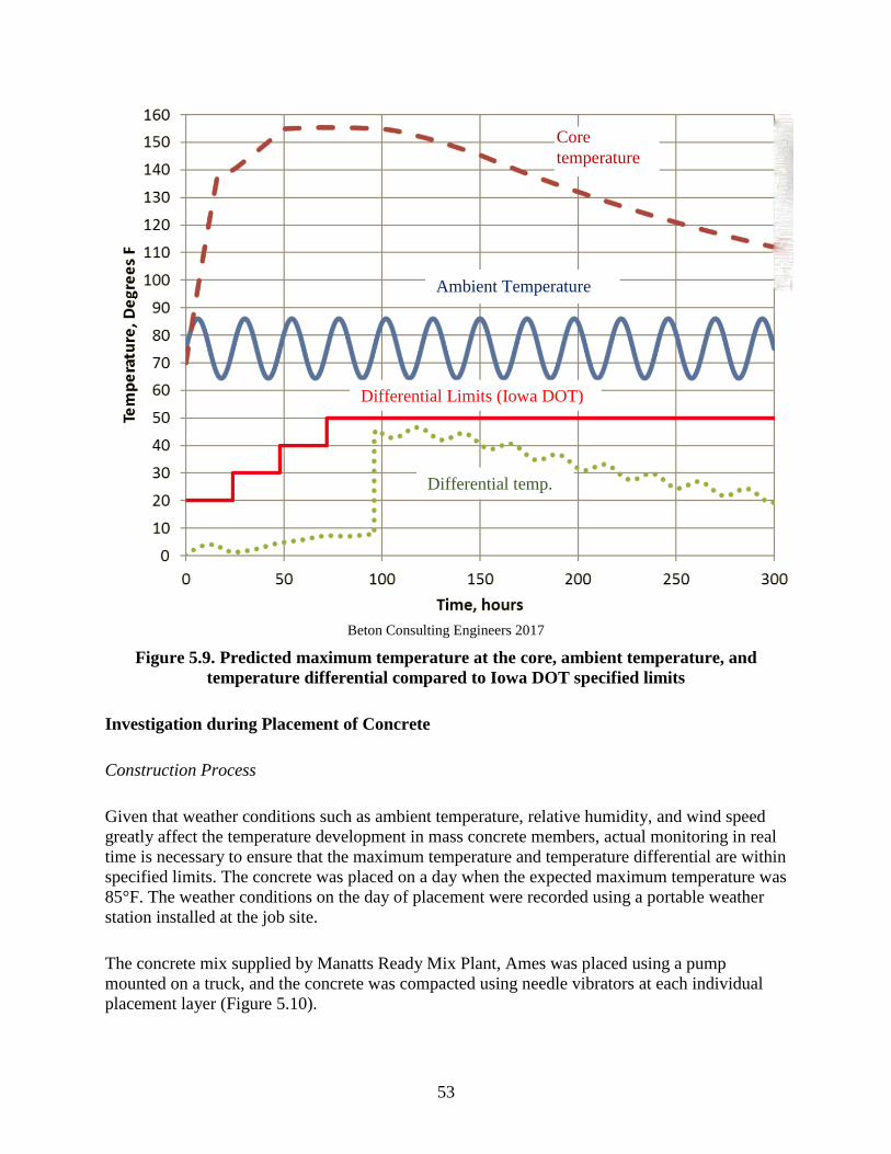
53
Beton Consulting Engineers 2017
Figure 5.9. Predicted maximum temperature at the core, ambient temperature, and
temperature differential compared to Iowa DOT specified limits
Investigation during Placement of Concrete
Construction Process
Given that weather conditions such as ambient temperature, relative humidity, and wind speed
greatly affect the temperature development in mass concrete members, actual monitoring in real
time is necessary to ensure that the maximum temperature and temperature differential are within
specified limits. The concrete was placed on a day when the expected maximum temperature was
85°F. The weather conditions on the day of placement were recorded using a portable weather
station installed at the job site.
The concrete mix supplied by Manatts Ready Mix Plant, Ames was placed using a pump
mounted on a truck, and the concrete was compacted using needle vibrators at each individual
placement layer (Figure 5.10).
Ambient Temperature
Differential Limits (Iowa DOT)
Differential temp.
Core
temperature
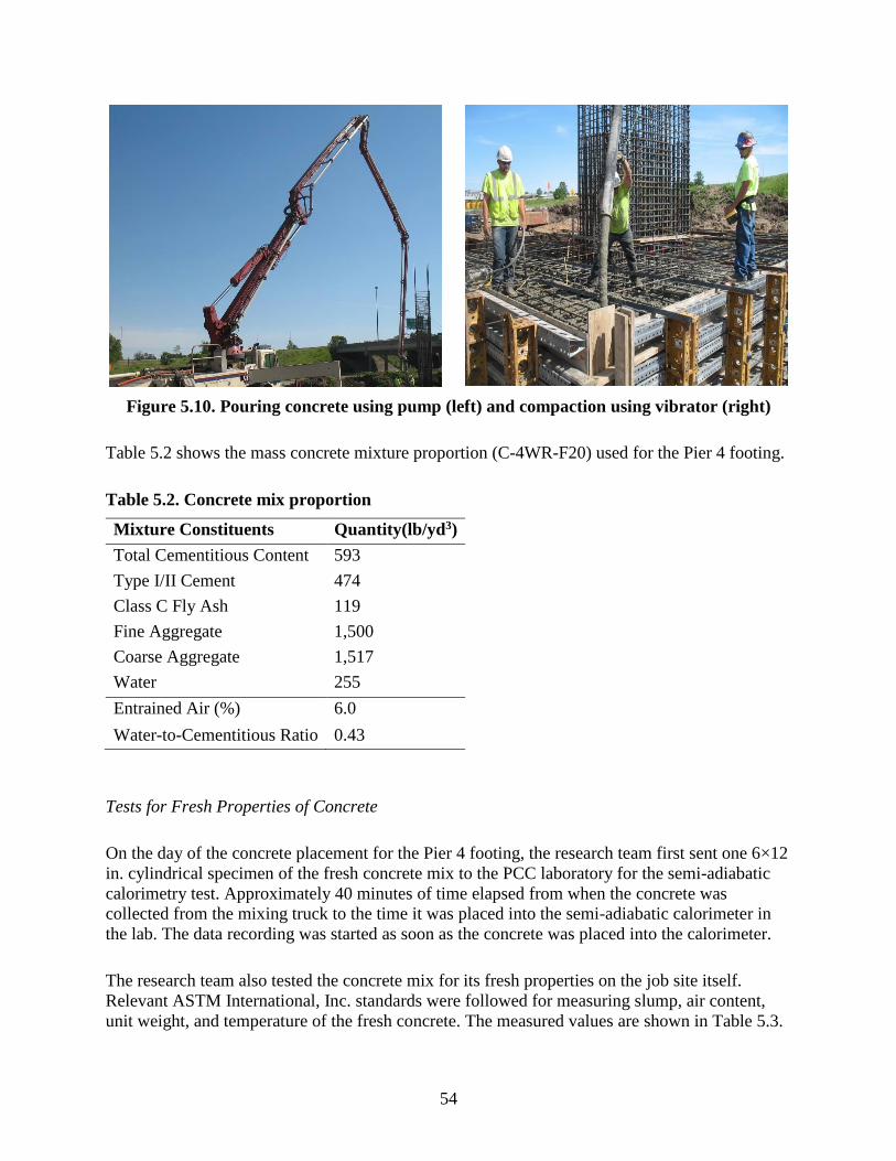
54
Figure 5.10. Pouring concrete using pump (left) and compaction using vibrator (right)
Table 5.2 shows the mass concrete mixture proportion (C-4WR-F20) used for the Pier 4 footing.
Table 5.2. Concrete mix proportion
Mixture Constituents Quantity(lb/yd3)
Total Cementitious Content 593
Type I/II Cement 474
Class C Fly Ash 119
Fine Aggregate 1,500
Coarse Aggregate 1,517
Water 255
Entrained Air (%) 6.0
Water-to-Cementitious Ratio 0.43
Tests for Fresh Properties of Concrete
On the day of the concrete placement for the Pier 4 footing, the research team first sent one 6×12
in. cylindrical specimen of the fresh concrete mix to the PCC laboratory for the semi-adiabatic
calorimetry test. Approximately 40 minutes of time elapsed from when the concrete was
collected from the mixing truck to the time it was placed into the semi-adiabatic calorimeter in
the lab. The data recording was started as soon as the concrete was placed into the calorimeter.
The research team also tested the concrete mix for its fresh properties on the job site itself.
Relevant ASTM International, Inc. standards were followed for measuring slump, air content,
unit weight, and temperature of the fresh concrete. The measured values are shown in Table 5.3.

55
Table 5.3. Fresh properties of Pier 4 footing concrete
Fresh Property Measured Value
Slump (in.) 2.75
Air Content (%) 7.5
Unit Weight (lb/ft3) 149.12
Temperature (°F) 63.6
Measured Weather Conditions
Weather conditions such as ambient temperature and relative humidity have an important impact
on the temperature development in a mass concrete member as well as on the hydration process
of cementitious materials. It was important to monitor the weather conditions on the day of the
placement of the concrete. For this purpose, a portable weather station was installed at the job
site for recording the temperature, relative humidity, and wind speed. Figure 5.11 shows the
installed weather station.
Figure 5.11. Weather station at job site
Casting of Specimens at Job Site
As planned, 40 cylindrical specimens of the field concrete mix were made at the job site by the
team. The specimens were cast so that the following tests could be performed in the laboratory at
various ages:
Compressive strength – maturity tests
Split tensile strength
Elastic modulus
Thermal conductivity
Coefficient of thermal expansion
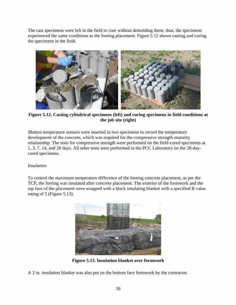
56
The cast specimens were left in the field to cure without demolding them; thus, the specimens
experienced the same conditions as the footing placement. Figure 5.12 shows casting and curing
the specimens in the field.
Figure 5.12. Casting cylindrical specimens (left) and curing specimens in field conditions at
the job site (right)
iButton temperature sensors were inserted in two specimens to record the temperature
development of the concrete, which was required for the compressive strength-maturity
relationship. The tests for compressive strength were performed on the field-cured specimens at
1, 3, 7, 14, and 28 days. All other tests were performed in the PCC Laboratory on the 28-day-
cured specimens.
Insulation
To control the maximum temperature difference of the footing concrete placement, as per the
TCP, the footing was insulated after concrete placement. The exterior of the formwork and the
top face of the placement were wrapped with a black insulating blanket with a specified R value
rating of 5 (Figure 5.13).
Figure 5.13. Insulation blanket over formwork
A 2 in. insulation blanket was also put on the bottom face formwork by the contractor.
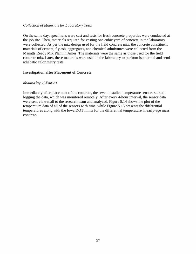
57
Collection of Materials for Laboratory Tests
On the same day, specimens were cast and tests for fresh concrete properties were conducted at
the job site. Then, materials required for casting one cubic yard of concrete in the laboratory
were collected. As per the mix design used for the field concrete mix, the concrete constituent
materials of cement, fly ash, aggregates, and chemical admixtures were collected from the
Manatts Ready Mix Plant in Ames. The materials were the same as those used for the field
concrete mix. Later, these materials were used in the laboratory to perform isothermal and semi-
adiabatic calorimetry tests.
Investigation after Placement of Concrete
Monitoring of Sensors
Immediately after placement of the concrete, the seven installed temperature sensors started
logging the data, which was monitored remotely. After every 4-hour interval, the sensor data
were sent via e-mail to the research team and analyzed. Figure 5.14 shows the plot of the
temperature data of all of the sensors with time, while Figure 5.15 presents the differential
temperatures along with the Iowa DOT limits for the differential temperature in early-age mass
concrete.
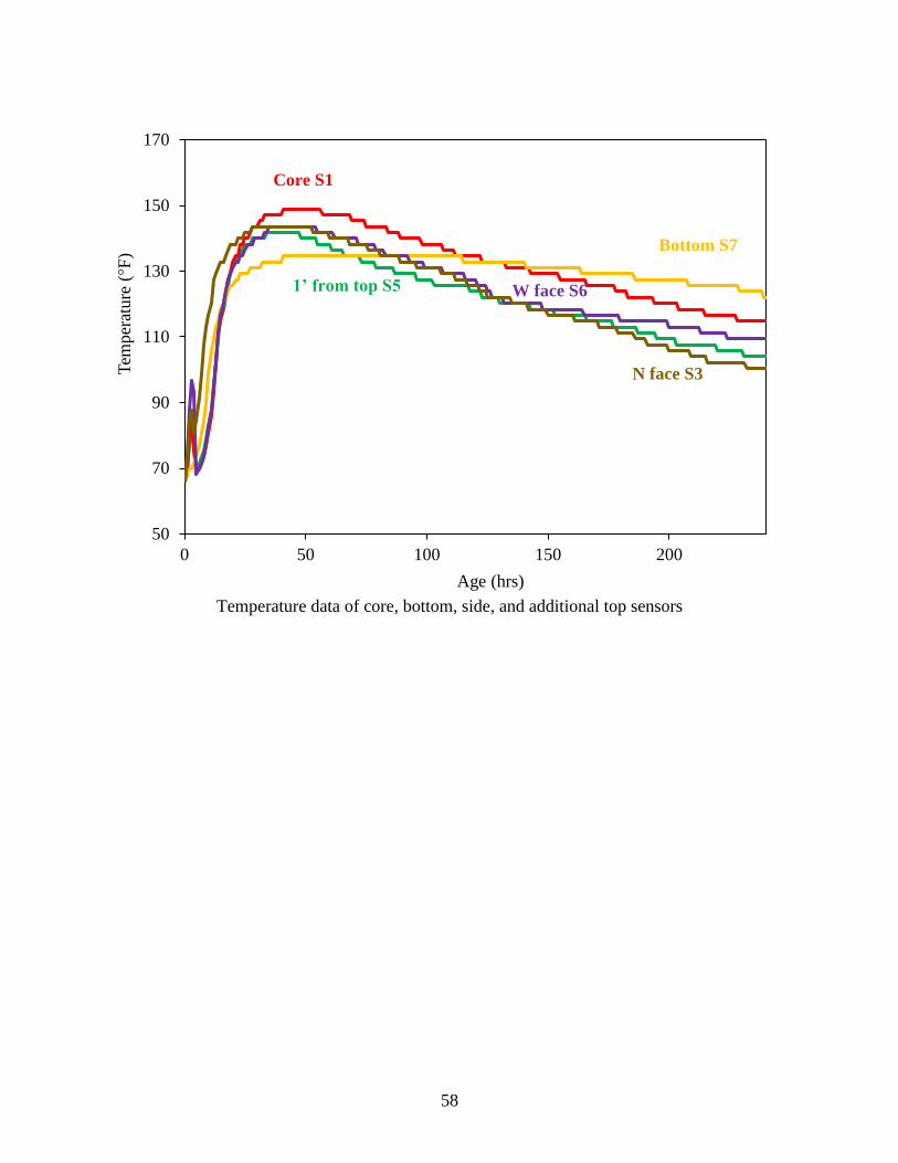
58
Temperature data of core, bottom, side, and additional top sensors
50
70
90
110
130
150
170
0 50 100 150 200
Tem
per
ature
(°F
)
Age (hrs)
Core S1
Bottom S7
W face S6
N face S3
1’ from top S5
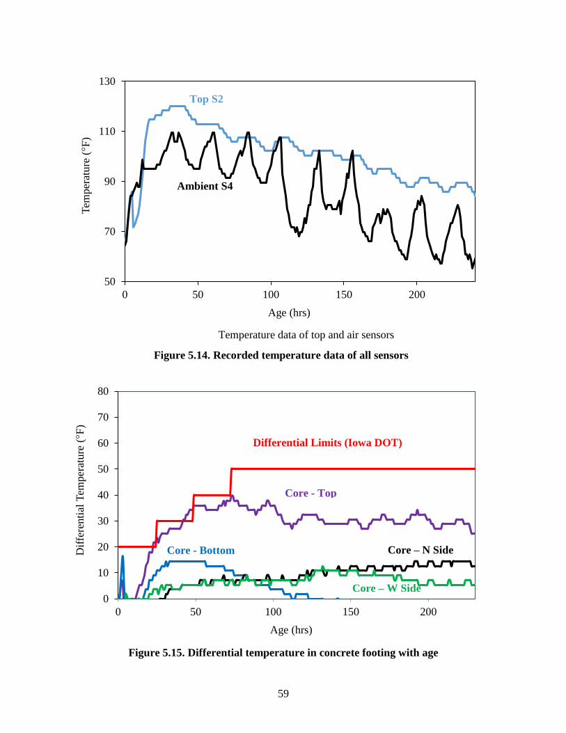
59
Temperature data of top and air sensors
Figure 5.14. Recorded temperature data of all sensors
Figure 5.15. Differential temperature in concrete footing with age
50
70
90
110
130
0 50 100 150 200
Tem
per
atu
re (
°F)
Age (hrs)
0
10
20
30
40
50
60
70
80
0 50 100 150 200
Dif
fere
nti
al T
emper
ature
(°F
)
Age (hrs)
Ambient S4
Top S2
Differential Limits (Iowa DOT)
Core - Top
Core – N Side
Core – W Side
Core - Bottom
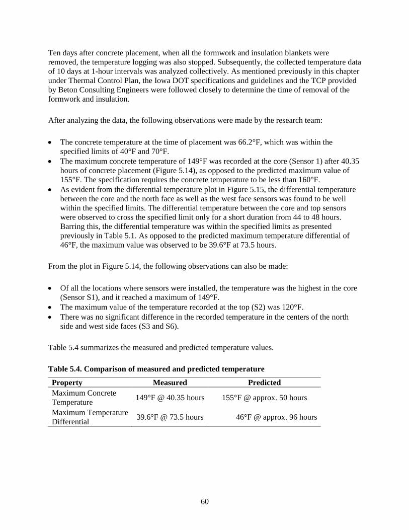
60
Ten days after concrete placement, when all the formwork and insulation blankets were
removed, the temperature logging was also stopped. Subsequently, the collected temperature data
of 10 days at 1-hour intervals was analyzed collectively. As mentioned previously in this chapter
under Thermal Control Plan, the Iowa DOT specifications and guidelines and the TCP provided
by Beton Consulting Engineers were followed closely to determine the time of removal of the
formwork and insulation.
After analyzing the data, the following observations were made by the research team:
The concrete temperature at the time of placement was 66.2°F, which was within the
specified limits of 40°F and 70°F.
The maximum concrete temperature of 149°F was recorded at the core (Sensor 1) after 40.35
hours of concrete placement (Figure 5.14), as opposed to the predicted maximum value of
155°F. The specification requires the concrete temperature to be less than 160°F.
As evident from the differential temperature plot in Figure 5.15, the differential temperature
between the core and the north face as well as the west face sensors was found to be well
within the specified limits. The differential temperature between the core and top sensors
were observed to cross the specified limit only for a short duration from 44 to 48 hours.
Barring this, the differential temperature was within the specified limits as presented
previously in Table 5.1. As opposed to the predicted maximum temperature differential of
46°F, the maximum value was observed to be 39.6°F at 73.5 hours.
From the plot in Figure 5.14, the following observations can also be made:
Of all the locations where sensors were installed, the temperature was the highest in the core
(Sensor S1), and it reached a maximum of 149°F.
The maximum value of the temperature recorded at the top (S2) was 120°F.
There was no significant difference in the recorded temperature in the centers of the north
side and west side faces (S3 and S6).
Table 5.4 summarizes the measured and predicted temperature values.
Table 5.4. Comparison of measured and predicted temperature
Property Measured Predicted
Maximum Concrete
Temperature 149°F @ 40.35 hours 155°F @ approx. 50 hours
Maximum Temperature
Differential 39.6°F @ 73.5 hours 46°F @ approx. 96 hours

61
Weather Conditions
The temperature, relative humidity, and wind speed were recorded using a portable weather
station on the day of the concrete placement. The weather fluctuations for 14 days after concrete
placement until the formwork and insulation were removed were monitored from available
online resources. The weather history database came from a weather station installed very near to
the job site in Ames by the Weather Underground (https://www.wunderground.com/), and it was
used to monitor the environmental conditions for the analysis period. The following data were
monitored each day:
Maximum and minimum temperature
Maximum and minimum relative humidity
Maximum wind speed
Rain and/or thunderstorm
The monitored conditions are presented in Table 5.5, while Figure 5.16 shows the plots for the
variation of temperature and relative humidity.
Table 5.5. Weather conditions at Pier 4 site
Date Day
Temperature
(°F)
Relative
Humidity (%) Max Wind
Speed (mph) Event Max Min Max Min
6/16/2017 0 87 64 93 55 16
6/17/2017 1 83 64 100 58 28 Rain
6/18/2017 2 79 57 93 43 24
6/19/2017 3 81 57 93 36 21
6/20/2017 4 90 54 100 24 24
6/21/2017 5 87 61 93 55 26
6/22/2017 6 87 70 93 51 26 Thunderstorm
6/23/2017 7 76 59 100 46 25
6/24/2017 8 78 53 86 24 28
6/25/2017 9 74 49 83 33 25
6/26/2017 10 74 48 100 35 17 Rain
6/27/2017 11 77 45 100 41 20
6/28/2017 12 84 65 93 65 30
6/29/2017 13 83 63 100 58 26
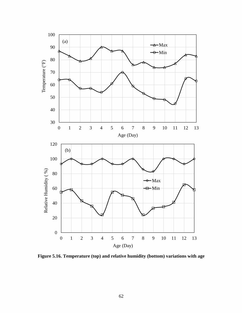
62
Figure 5.16. Temperature (top) and relative humidity (bottom) variations with age
30
40
50
60
70
80
90
100
0 1 2 3 4 5 6 7 8 9 10 11 12 13
Tem
per
ature
(°F
)
Age (Day)
(a)Max
Min
0
20
40
60
80
100
120
0 1 2 3 4 5 6 7 8 9 10 11 12 13
Rel
ativ
e H
um
idit
y (
%)
Age (Day)
(b)
Max
Min
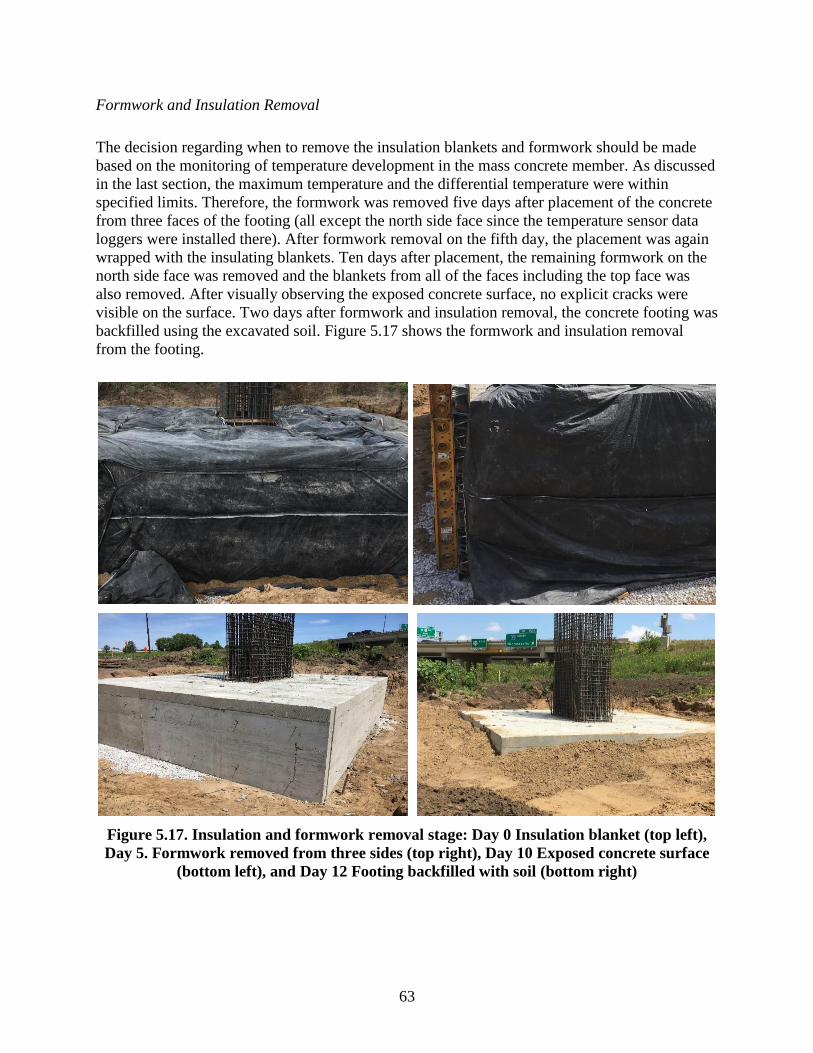
63
Formwork and Insulation Removal
The decision regarding when to remove the insulation blankets and formwork should be made
based on the monitoring of temperature development in the mass concrete member. As discussed
in the last section, the maximum temperature and the differential temperature were within
specified limits. Therefore, the formwork was removed five days after placement of the concrete
from three faces of the footing (all except the north side face since the temperature sensor data
loggers were installed there). After formwork removal on the fifth day, the placement was again
wrapped with the insulating blankets. Ten days after placement, the remaining formwork on the
north side face was removed and the blankets from all of the faces including the top face was
also removed. After visually observing the exposed concrete surface, no explicit cracks were
visible on the surface. Two days after formwork and insulation removal, the concrete footing was
backfilled using the excavated soil. Figure 5.17 shows the formwork and insulation removal
from the footing.
Figure 5.17. Insulation and formwork removal stage: Day 0 Insulation blanket (top left),
Day 5. Formwork removed from three sides (top right), Day 10 Exposed concrete surface
(bottom left), and Day 12 Footing backfilled with soil (bottom right)
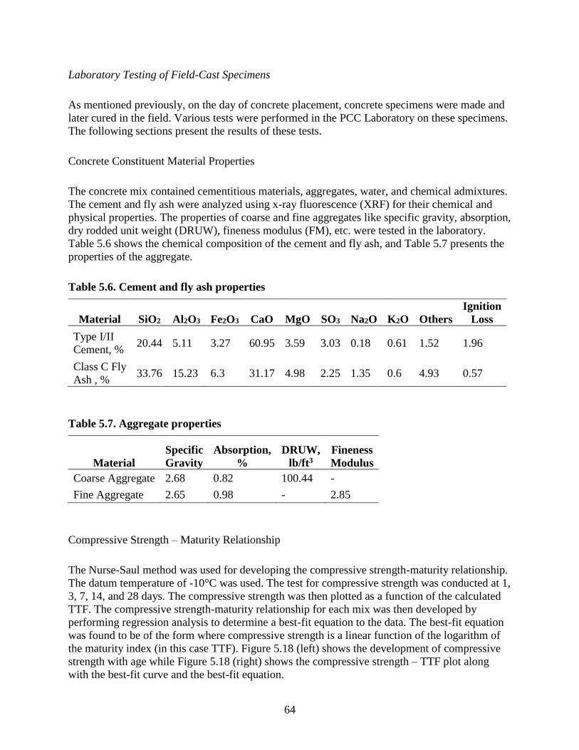
64
Laboratory Testing of Field-Cast Specimens
As mentioned previously, on the day of concrete placement, concrete specimens were made and
later cured in the field. Various tests were performed in the PCC Laboratory on these specimens.
The following sections present the results of these tests.
Concrete Constituent Material Properties
The concrete mix contained cementitious materials, aggregates, water, and chemical admixtures.
The cement and fly ash were analyzed using x-ray fluorescence (XRF) for their chemical and
physical properties. The properties of coarse and fine aggregates like specific gravity, absorption,
dry rodded unit weight (DRUW), fineness modulus (FM), etc. were tested in the laboratory.
Table 5.6 shows the chemical composition of the cement and fly ash, and Table 5.7 presents the
properties of the aggregate.
Table 5.6. Cement and fly ash properties
Material SiO2 Al2O3 Fe2O3 CaO MgO SO3 Na2O K2O Others
Ignition
Loss
Type I/II
Cement, % 20.44 5.11 3.27 60.95 3.59 3.03 0.18 0.61 1.52 1.96
Class C Fly
Ash , % 33.76 15.23 6.3 31.17 4.98 2.25 1.35 0.6 4.93 0.57
Table 5.7. Aggregate properties
Material
Specific
Gravity
Absorption,
%
DRUW,
lb/ft3
Fineness
Modulus
Coarse Aggregate 2.68 0.82 100.44 -
Fine Aggregate 2.65 0.98 - 2.85
Compressive Strength – Maturity Relationship
The Nurse-Saul method was used for developing the compressive strength-maturity relationship.
The datum temperature of -10°C was used. The test for compressive strength was conducted at 1,
3, 7, 14, and 28 days. The compressive strength was then plotted as a function of the calculated
TTF. The compressive strength-maturity relationship for each mix was then developed by
performing regression analysis to determine a best-fit equation to the data. The best-fit equation
was found to be of the form where compressive strength is a linear function of the logarithm of
the maturity index (in this case TTF). Figure 5.18 (left) shows the development of compressive
strength with age while Figure 5.18 (right) shows the compressive strength – TTF plot along
with the best-fit curve and the best-fit equation.
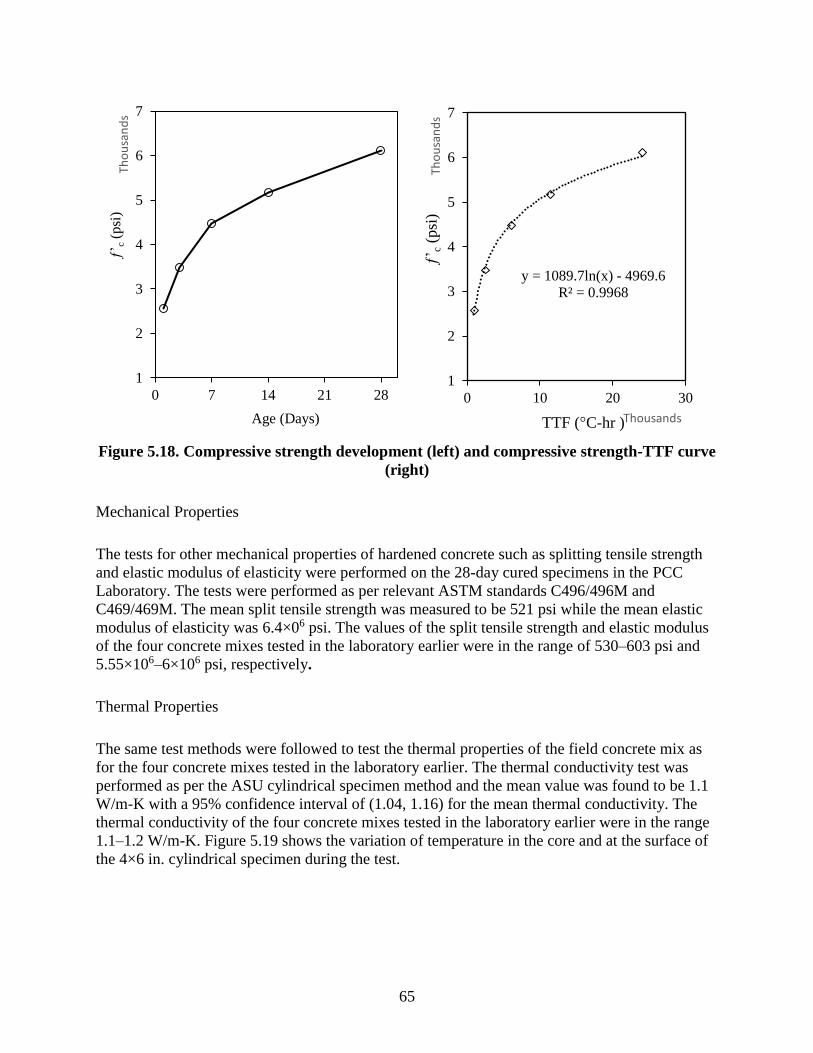
65
Figure 5.18. Compressive strength development (left) and compressive strength-TTF curve
(right)
Mechanical Properties
The tests for other mechanical properties of hardened concrete such as splitting tensile strength
and elastic modulus of elasticity were performed on the 28-day cured specimens in the PCC
Laboratory. The tests were performed as per relevant ASTM standards C496/496M and
C469/469M. The mean split tensile strength was measured to be 521 psi while the mean elastic
modulus of elasticity was 6.4×06 psi. The values of the split tensile strength and elastic modulus
of the four concrete mixes tested in the laboratory earlier were in the range of 530–603 psi and
5.55×10⁶–6×10⁶ psi, respectively.
Thermal Properties
The same test methods were followed to test the thermal properties of the field concrete mix as
for the four concrete mixes tested in the laboratory earlier. The thermal conductivity test was
performed as per the ASU cylindrical specimen method and the mean value was found to be 1.1
W/m-K with a 95% confidence interval of (1.04, 1.16) for the mean thermal conductivity. The
thermal conductivity of the four concrete mixes tested in the laboratory earlier were in the range
1.1–1.2 W/m-K. Figure 5.19 shows the variation of temperature in the core and at the surface of
the 4×6 in. cylindrical specimen during the test.
1
2
3
4
5
6
7
0 7 14 21 28
’ c
(psi
)Th
ou
san
ds
Age (Days)
y = 1089.7ln(x) - 4969.6
R² = 0.9968
1
2
3
4
5
6
7
0 10 20 30
’ c
(psi
)Th
ou
san
ds
TTF (°C-hr )Thousands
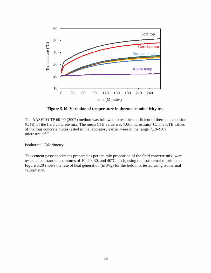
66
Figure 5.19. Variation of temperature in thermal conductivity test
The AASHTO TP 60-00 (2007) method was followed to test the coefficient of thermal expansion
(CTE) of the field concrete mix. The mean CTE value was 7.06 microstrain/°C. The CTE values
of the four concrete mixes tested in the laboratory earlier were in the range 7.19–9.07
microstrain/°C.
Isothermal Calorimetry
The cement paste specimens prepared as per the mix proportion of the field concrete mix, were
tested at constant temperatures of 10, 20, 30, and 40°C, each, using the isothermal calorimeter.
Figure 5.20 shows the rate of heat generation (mW/g) for the field mix tested using isothermal
calorimetry.
10
20
30
40
50
60
0 30 60 90 120 150 180 210 240
Tem
per
ature
(°C
)
Time (Minutes)
Core bottom
Core top
Surface temp.
Room temp.
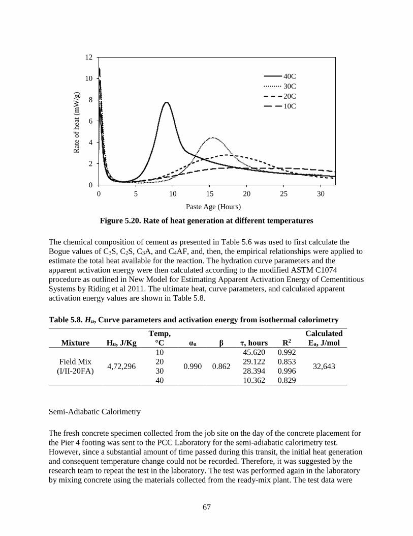
67
Figure 5.20. Rate of heat generation at different temperatures
The chemical composition of cement as presented in Table 5.6 was used to first calculate the
Bogue values of C3S, C2S, C3A, and C4AF, and, then, the empirical relationships were applied to
estimate the total heat available for the reaction. The hydration curve parameters and the
apparent activation energy were then calculated according to the modified ASTM C1074
procedure as outlined in New Model for Estimating Apparent Activation Energy of Cementitious
Systems by Riding et al 2011. The ultimate heat, curve parameters, and calculated apparent
activation energy values are shown in Table 5.8.
Table 5.8. Hu, Curve parameters and activation energy from isothermal calorimetry
Mixture Hu, J/Kg
Temp,
°C αu β τ, hours R2
Calculated
Ea, J/mol
Field Mix
(I/II-20FA) 4,72,296
10
0.990 0.862
45.620 0.992
32,643 20 29.122 0.853
30 28.394 0.996
40 10.362 0.829
Semi-Adiabatic Calorimetry
The fresh concrete specimen collected from the job site on the day of the concrete placement for
the Pier 4 footing was sent to the PCC Laboratory for the semi-adiabatic calorimetry test.
However, since a substantial amount of time passed during this transit, the initial heat generation
and consequent temperature change could not be recorded. Therefore, it was suggested by the
research team to repeat the test in the laboratory. The test was performed again in the laboratory
by mixing concrete using the materials collected from the ready-mix plant. The test data were
0
2
4
6
8
10
12
0 5 10 15 20 25 30
Rat
e o
f h
eat
(mW
/g)
Paste Age (Hours)
40C
30C
20C
10C
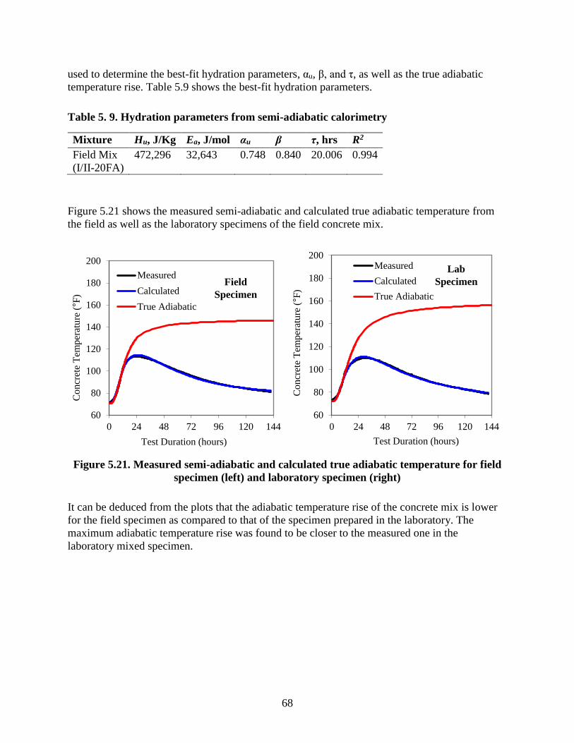
68
used to determine the best-fit hydration parameters, αu, β, and τ, as well as the true adiabatic
temperature rise. Table 5.9 shows the best-fit hydration parameters.
Table 5. 9. Hydration parameters from semi-adiabatic calorimetry
Mixture Hu, J/Kg Ea, J/mol αu β τ, hrs R2
Field Mix
(I/II-20FA)
472,296 32,643 0.748 0.840 20.006 0.994
Figure 5.21 shows the measured semi-adiabatic and calculated true adiabatic temperature from
the field as well as the laboratory specimens of the field concrete mix.
Figure 5.21. Measured semi-adiabatic and calculated true adiabatic temperature for field
specimen (left) and laboratory specimen (right)
It can be deduced from the plots that the adiabatic temperature rise of the concrete mix is lower
for the field specimen as compared to that of the specimen prepared in the laboratory. The
maximum adiabatic temperature rise was found to be closer to the measured one in the
laboratory mixed specimen.
60
80
100
120
140
160
180
200
0 24 48 72 96 120 144
Concr
ete
Tem
per
ature
(°F
)
Test Duration (hours)
Measured
Calculated
True Adiabatic
Field
Specimen
60
80
100
120
140
160
180
200
0 24 48 72 96 120 144
Concr
ete
Tem
per
ature
(°F
)
Test Duration (hours)
Measured
Calculated
True Adiabatic
Lab
Specimen
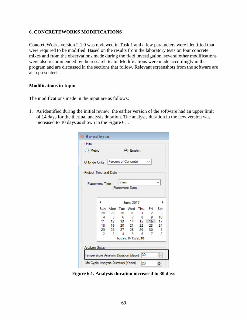
69
6. CONCRETEWORKS MODIFICATIONS
ConcreteWorks version 2.1.0 was reviewed in Task 1 and a few parameters were identified that
were required to be modified. Based on the results from the laboratory tests on four concrete
mixes and from the observations made during the field investigation, several other modifications
were also recommended by the research team. Modifications were made accordingly in the
program and are discussed in the sections that follow. Relevant screenshots from the software are
also presented.
Modifications in Input
The modifications made in the input are as follows:
1. As identified during the initial review, the earlier version of the software had an upper limit
of 14 days for the thermal analysis duration. The analysis duration in the new version was
increased to 30 days as shown in the Figure 6.1.
Figure 6.1. Analysis duration increased to 30 days
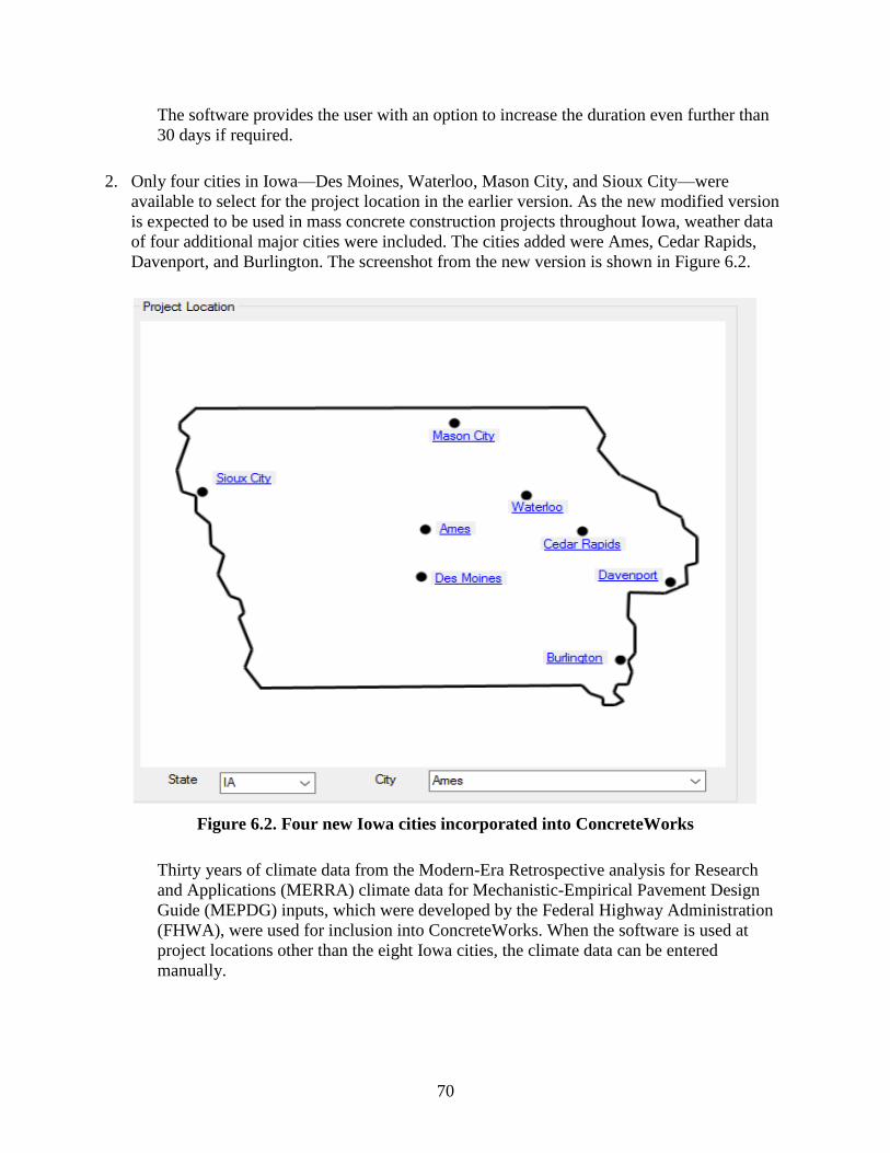
70
The software provides the user with an option to increase the duration even further than
30 days if required.
2. Only four cities in Iowa—Des Moines, Waterloo, Mason City, and Sioux City—were
available to select for the project location in the earlier version. As the new modified version
is expected to be used in mass concrete construction projects throughout Iowa, weather data
of four additional major cities were included. The cities added were Ames, Cedar Rapids,
Davenport, and Burlington. The screenshot from the new version is shown in Figure 6.2.
Figure 6.2. Four new Iowa cities incorporated into ConcreteWorks
Thirty years of climate data from the Modern-Era Retrospective analysis for Research
and Applications (MERRA) climate data for Mechanistic-Empirical Pavement Design
Guide (MEPDG) inputs, which were developed by the Federal Highway Administration
(FHWA), were used for inclusion into ConcreteWorks. When the software is used at
project locations other than the eight Iowa cities, the climate data can be entered
manually.
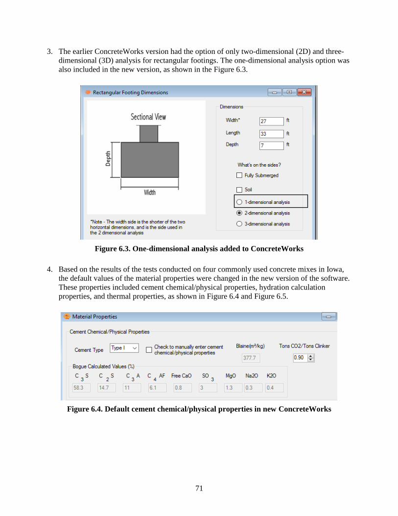
71
3. The earlier ConcreteWorks version had the option of only two-dimensional (2D) and three-
dimensional (3D) analysis for rectangular footings. The one-dimensional analysis option was
also included in the new version, as shown in the Figure 6.3.
Figure 6.3. One-dimensional analysis added to ConcreteWorks
4. Based on the results of the tests conducted on four commonly used concrete mixes in Iowa,
the default values of the material properties were changed in the new version of the software.
These properties included cement chemical/physical properties, hydration calculation
properties, and thermal properties, as shown in Figure 6.4 and Figure 6.5.
Figure 6.4. Default cement chemical/physical properties in new ConcreteWorks
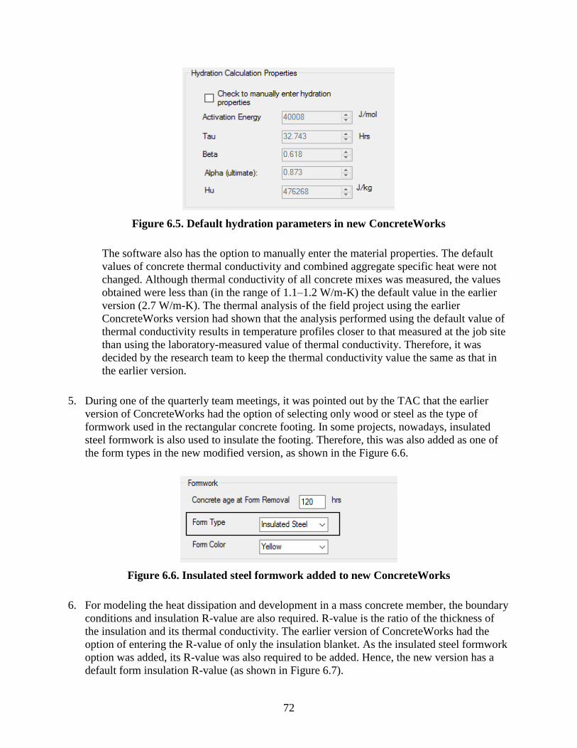
72
Figure 6.5. Default hydration parameters in new ConcreteWorks
The software also has the option to manually enter the material properties. The default
values of concrete thermal conductivity and combined aggregate specific heat were not
changed. Although thermal conductivity of all concrete mixes was measured, the values
obtained were less than (in the range of 1.1–1.2 W/m-K) the default value in the earlier
version (2.7 W/m-K). The thermal analysis of the field project using the earlier
ConcreteWorks version had shown that the analysis performed using the default value of
thermal conductivity results in temperature profiles closer to that measured at the job site
than using the laboratory-measured value of thermal conductivity. Therefore, it was
decided by the research team to keep the thermal conductivity value the same as that in
the earlier version.
5. During one of the quarterly team meetings, it was pointed out by the TAC that the earlier
version of ConcreteWorks had the option of selecting only wood or steel as the type of
formwork used in the rectangular concrete footing. In some projects, nowadays, insulated
steel formwork is also used to insulate the footing. Therefore, this was also added as one of
the form types in the new modified version, as shown in the Figure 6.6.
Figure 6.6. Insulated steel formwork added to new ConcreteWorks
6. For modeling the heat dissipation and development in a mass concrete member, the boundary
conditions and insulation R-value are also required. R-value is the ratio of the thickness of
the insulation and its thermal conductivity. The earlier version of ConcreteWorks had the
option of entering the R-value of only the insulation blanket. As the insulated steel formwork
option was added, its R-value was also required to be added. Hence, the new version has a
default form insulation R-value (as shown in Figure 6.7).
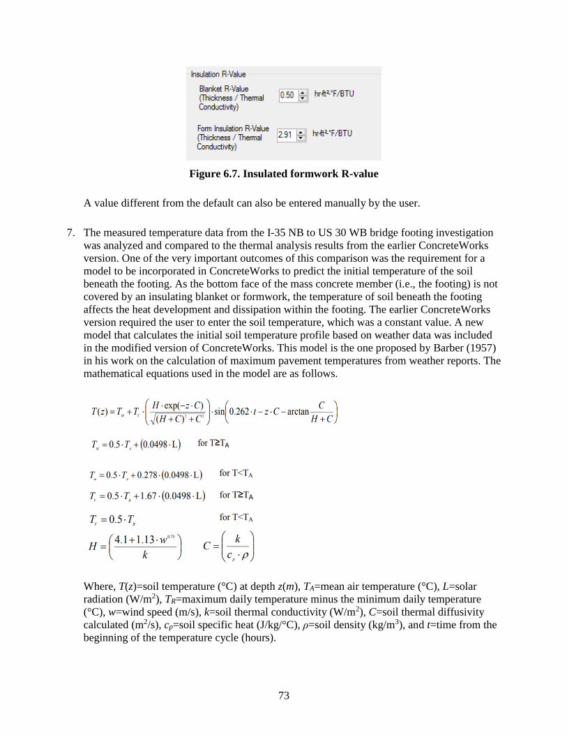
73
Figure 6.7. Insulated formwork R-value
A value different from the default can also be entered manually by the user.
7. The measured temperature data from the I-35 NB to US 30 WB bridge footing investigation
was analyzed and compared to the thermal analysis results from the earlier ConcreteWorks
version. One of the very important outcomes of this comparison was the requirement for a
model to be incorporated in ConcreteWorks to predict the initial temperature of the soil
beneath the footing. As the bottom face of the mass concrete member (i.e., the footing) is not
covered by an insulating blanket or formwork, the temperature of soil beneath the footing
affects the heat development and dissipation within the footing. The earlier ConcreteWorks
version required the user to enter the soil temperature, which was a constant value. A new
model that calculates the initial soil temperature profile based on weather data was included
in the modified version of ConcreteWorks. This model is the one proposed by Barber (1957)
in his work on the calculation of maximum pavement temperatures from weather reports. The
mathematical equations used in the model are as follows.
Where, T(z)=soil temperature (°C) at depth z(m), TA=mean air temperature (°C), L=solar
radiation (W/m2), TR=maximum daily temperature minus the minimum daily temperature
(°C), w=wind speed (m/s), k=soil thermal conductivity (W/m2), C=soil thermal diffusivity
calculated (m2/s), cp=soil specific heat (J/kg/°C), ρ=soil density (kg/m3), and t=time from the
beginning of the temperature cycle (hours).
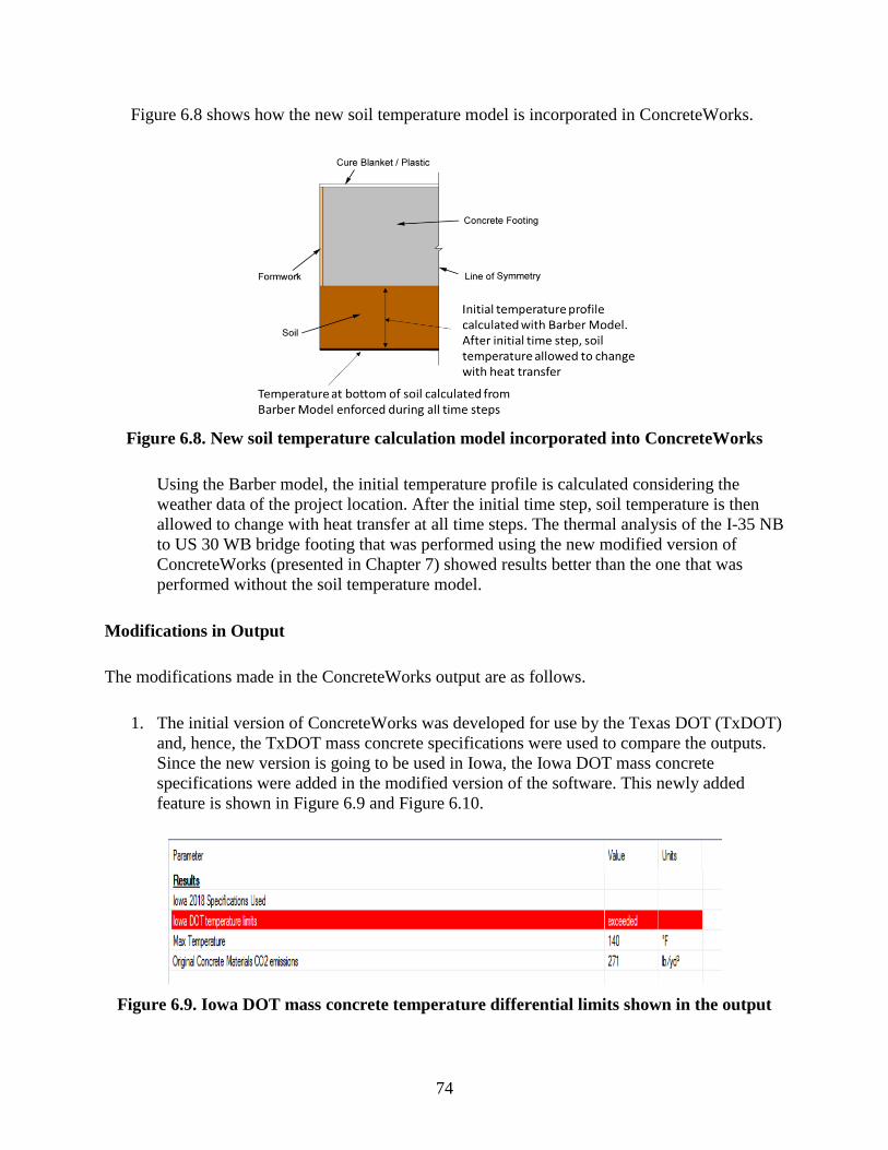
74
Figure 6.8 shows how the new soil temperature model is incorporated in ConcreteWorks.
Figure 6.8. New soil temperature calculation model incorporated into ConcreteWorks
Using the Barber model, the initial temperature profile is calculated considering the
weather data of the project location. After the initial time step, soil temperature is then
allowed to change with heat transfer at all time steps. The thermal analysis of the I-35 NB
to US 30 WB bridge footing that was performed using the new modified version of
ConcreteWorks (presented in Chapter 7) showed results better than the one that was
performed without the soil temperature model.
Modifications in Output
The modifications made in the ConcreteWorks output are as follows.
1. The initial version of ConcreteWorks was developed for use by the Texas DOT (TxDOT)
and, hence, the TxDOT mass concrete specifications were used to compare the outputs.
Since the new version is going to be used in Iowa, the Iowa DOT mass concrete
specifications were added in the modified version of the software. This newly added
feature is shown in Figure 6.9 and Figure 6.10.
Figure 6.9. Iowa DOT mass concrete temperature differential limits shown in the output
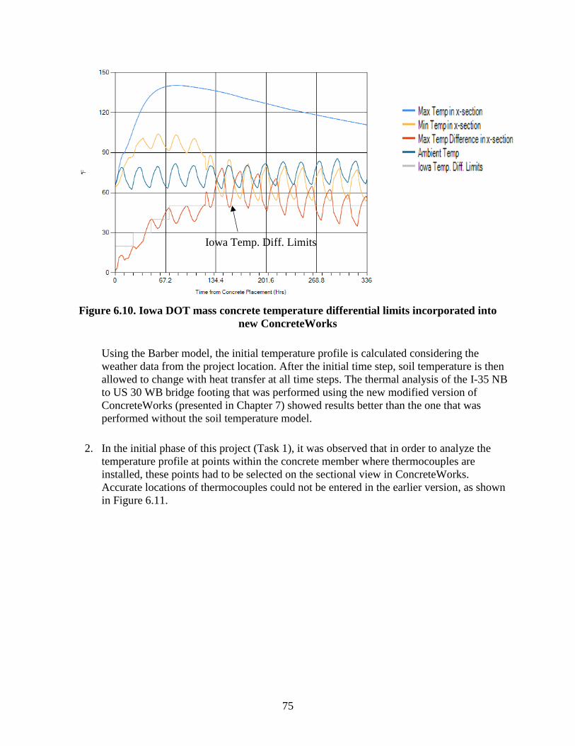
75
Figure 6.10. Iowa DOT mass concrete temperature differential limits incorporated into
new ConcreteWorks
Using the Barber model, the initial temperature profile is calculated considering the
weather data from the project location. After the initial time step, soil temperature is then
allowed to change with heat transfer at all time steps. The thermal analysis of the I-35 NB
to US 30 WB bridge footing that was performed using the new modified version of
ConcreteWorks (presented in Chapter 7) showed results better than the one that was
performed without the soil temperature model.
2. In the initial phase of this project (Task 1), it was observed that in order to analyze the
temperature profile at points within the concrete member where thermocouples are
installed, these points had to be selected on the sectional view in ConcreteWorks.
Accurate locations of thermocouples could not be entered in the earlier version, as shown
in Figure 6.11.
Iowa Temp. Diff. Limits
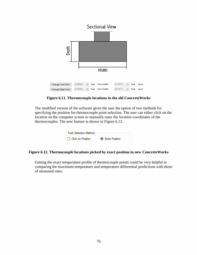
76
Figure 6.11. Thermocouple locations in the old ConcreteWorks
The modified version of the software gives the user the option of two methods for
specifying the position for thermocouple point selection. The user can either click on the
location on the computer screen or manually enter the location coordinates of the
thermocouples. The new feature is shown in Figure 6.12.
Figure 6.12. Thermocouple locations picked by exact position in new ConcreteWorks
Getting the exact temperature profile of thermocouple points could be very helpful in
comparing the maximum temperature and temperature differential predictions with those
of measured ones.
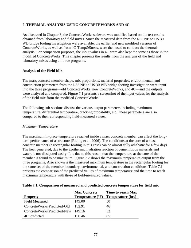
77
7. THERMAL ANALYSIS USING CONCRETEWORKS AND 4C
As discussed in Chapter 6, the ConcreteWorks software was modified based on the test results
obtained from laboratory and field mixes. Since the measured data from the I-35 NB to US 30
WB bridge footing investigation were available, the earlier and new modified versions of
ConcreteWorks, as well as from 4C-Temp&Stress, were then used to conduct the thermal
analysis. For comparison purposes, the input values in 4C were also kept the same as those in the
modified ConcreteWorks. This chapter presents the results from the analysis of the field and
laboratory mixes using all three programs.
Analysis of the Field Mix
The mass concrete member shape, mix proportions, material properties, environmental, and
construction parameters from the I-35 NB to US 30 WB bridge footing investigation were input
into the three programs—old ConcreteWorks, new ConcreteWorks, and 4C—and the outputs
were analyzed and compared. Figure 7.1 presents a screenshot of the input values for the analysis
of the field mix from the modified ConcreteWorks.
The following sub-sections discuss the various output parameters including maximum
temperature, differential temperature, cracking probability, etc. These parameters are also
compared to their corresponding field-measured values.
Maximum Temperature
The maximum in-place temperature reached inside a mass concrete member can affect the long-
term performance of a structure (Riding et al. 2006). The conditions at the core of a mass
concrete member (a rectangular footing in this case) can be almost fully adiabatic for a few days.
The heat generated, due to the exothermic hydration reaction of cementitious materials and
water, is not dissipated easily. It is due to this reason that the temperature at the core of the
member is found to be maximum. Figure 7.2 shows the maximum temperature output from the
three programs. Also shown is the measured maximum temperature in the rectangular footing for
the same set of the member, boundary, environmental, and construction conditions. Table 7.1
presents the comparison of the predicted values of maximum temperature and the time to reach
maximum temperature with those of field-measured values.
Table 7.1. Comparison of measured and predicted concrete temperature for field mix
Property
Max Concrete
Temperature (°F)
Time to reach Max
Temperature (hrs)
Field Measured 149.00 50
ConcreteWorks Predicted-Old 152.91 46
ConcreteWorks Predicted-New 149.16 52
4C Predicted 150.46 65
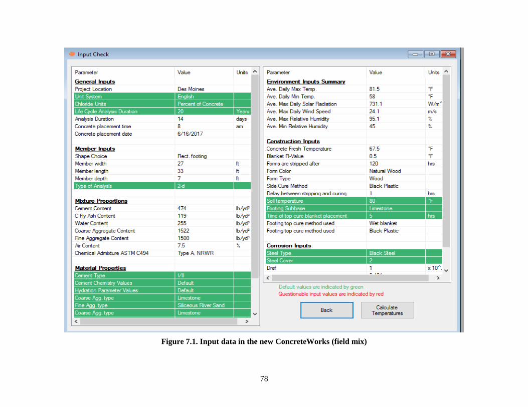
78
Figure 7.1. Input data in the new ConcreteWorks (field mix)
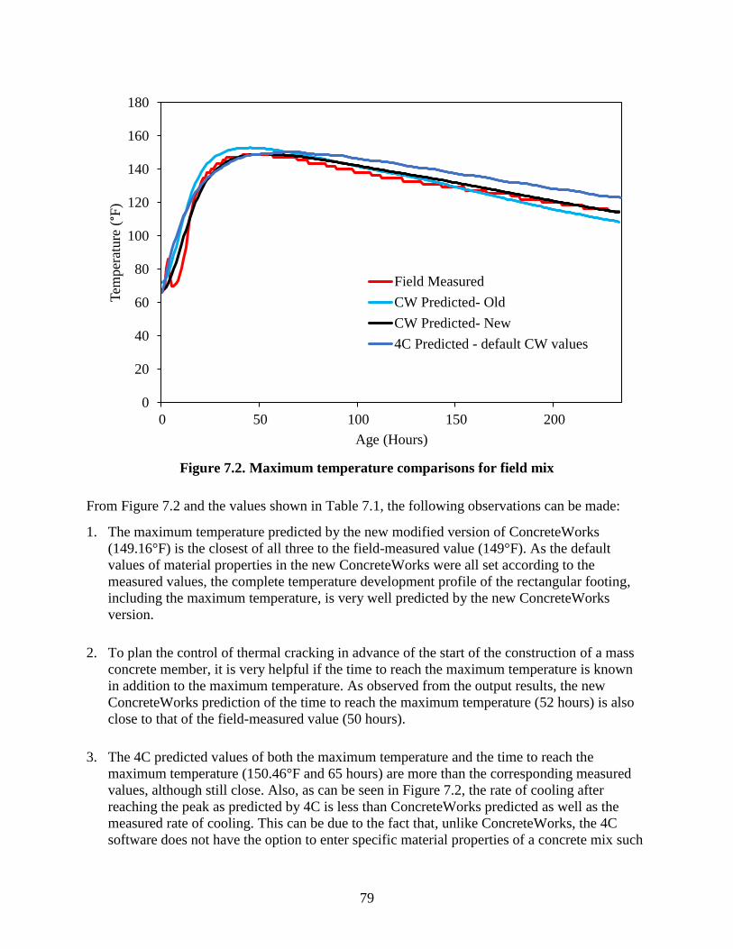
79
Figure 7.2. Maximum temperature comparisons for field mix
From Figure 7.2 and the values shown in Table 7.1, the following observations can be made:
1. The maximum temperature predicted by the new modified version of ConcreteWorks
(149.16°F) is the closest of all three to the field-measured value (149°F). As the default
values of material properties in the new ConcreteWorks were all set according to the
measured values, the complete temperature development profile of the rectangular footing,
including the maximum temperature, is very well predicted by the new ConcreteWorks
version.
2. To plan the control of thermal cracking in advance of the start of the construction of a mass
concrete member, it is very helpful if the time to reach the maximum temperature is known
in addition to the maximum temperature. As observed from the output results, the new
ConcreteWorks prediction of the time to reach the maximum temperature (52 hours) is also
close to that of the field-measured value (50 hours).
3. The 4C predicted values of both the maximum temperature and the time to reach the
maximum temperature (150.46°F and 65 hours) are more than the corresponding measured
values, although still close. Also, as can be seen in Figure 7.2, the rate of cooling after
reaching the peak as predicted by 4C is less than ConcreteWorks predicted as well as the
measured rate of cooling. This can be due to the fact that, unlike ConcreteWorks, the 4C
software does not have the option to enter specific material properties of a concrete mix such
0
20
40
60
80
100
120
140
160
180
0 50 100 150 200
Tem
per
atu
re (°F
)
Age (Hours)
Field Measured
CW Predicted- Old
CW Predicted- New
4C Predicted - default CW values

80
as the type of mineral admixture used, the chemical/physical properties of cementitious
materials, etc.
Temperature at Thermocouple Locations
Seven sets of intelliRock temperature sensors were installed in the rectangular footing before the
concrete placement (as discussed in Chapter 5). The sensors were installed to monitor the
temperature development at seven designated locations on the footing and take relevant measures
for its thermal crack control. The locations analyzed within the rectangular footing were core,
top, 1 ft from the top, bottom, north face, and south face. The seventh sensor was placed outside
the footing to measure the ambient temperature.
Usually, in rectangular footings, which qualify as mass concrete, only three locations are critical
from the perspective of thermal cracking. These locations are core, top, and the center of the face
at the smallest distance from the core of the member. For the purpose of refining the prediction
model in ConcreteWorks, the temperatures at additional locations such as 1 ft from the top,
bottom, and the center of the face at the largest distance from the core were also analyzed.
One of the most important features in ConcreteWorks is that it provides the user with an option
to get the temperature development profile of any point within the mass concrete member. The
finite element mesh in 4C can also be used to analyze the same. The three computer programs
were used to obtain the temperature profile at all of the locations where the sensors were
installed and the outputs were then compared with the measured values. The comparison charts
of the temperature profiles at all sensor locations are shown in Figure 7.3.
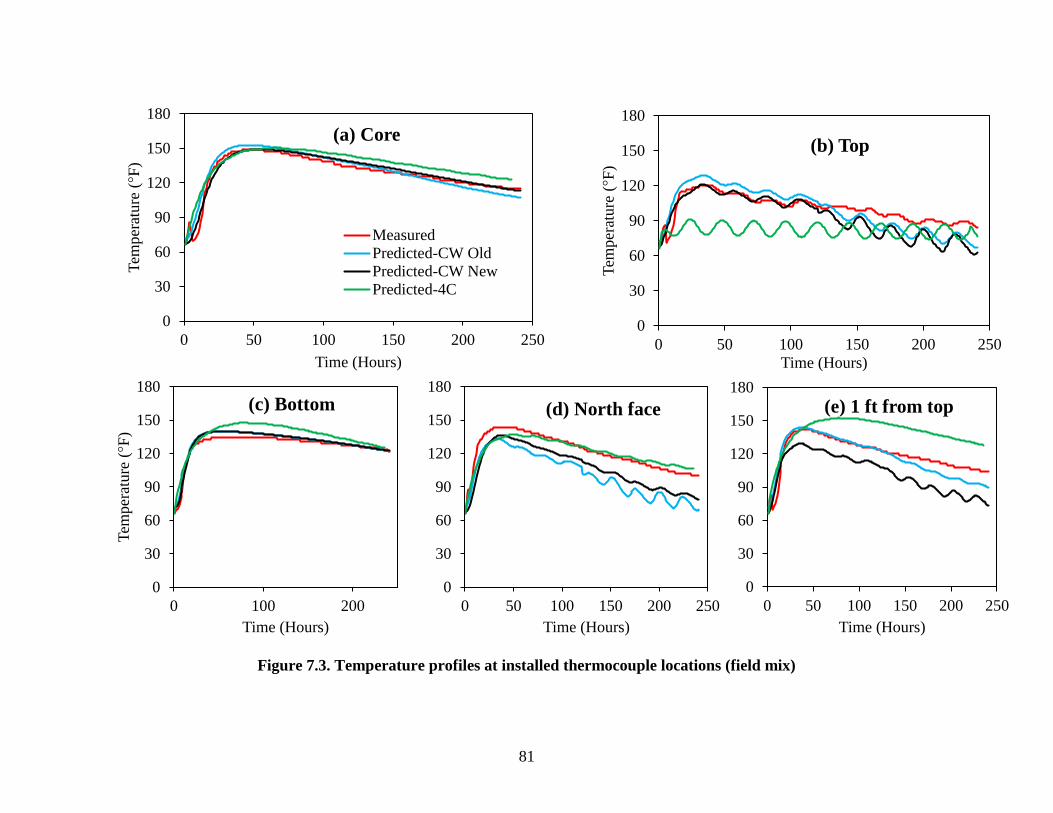
81
Figure 7.3. Temperature profiles at installed thermocouple locations (field mix)
0
30
60
90
120
150
180
0 50 100 150 200 250
Tem
per
ature
(°F
)
Time (Hours)
(a) Core
MeasuredPredicted-CW OldPredicted-CW New
Predicted-4C
0
30
60
90
120
150
180
0 50 100 150 200 250
Tem
per
ature
(°F
)
Time (Hours)
(b) Top
0
30
60
90
120
150
180
0 100 200
Tem
per
ature
(°F
)
Time (Hours)
(c) Bottom
0
30
60
90
120
150
180
0 50 100 150 200 250
Time (Hours)
(d) North face
0
30
60
90
120
150
180
0 50 100 150 200 250
Time (Hours)
(e) 1 ft from top
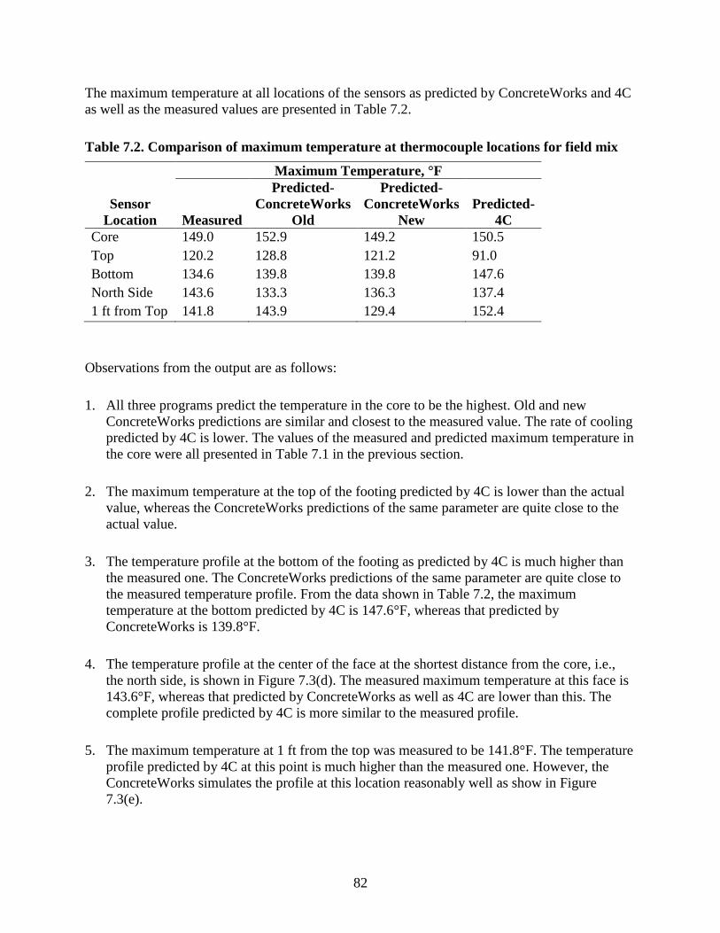
82
The maximum temperature at all locations of the sensors as predicted by ConcreteWorks and 4C
as well as the measured values are presented in Table 7.2.
Table 7.2. Comparison of maximum temperature at thermocouple locations for field mix
Sensor
Location
Maximum Temperature, °F
Measured
Predicted-
ConcreteWorks
Old
Predicted-
ConcreteWorks
New
Predicted-
4C
Core 149.0 152.9 149.2 150.5
Top 120.2 128.8 121.2 91.0
Bottom 134.6 139.8 139.8 147.6
North Side 143.6 133.3 136.3 137.4
1 ft from Top 141.8 143.9 129.4 152.4
Observations from the output are as follows:
1. All three programs predict the temperature in the core to be the highest. Old and new
ConcreteWorks predictions are similar and closest to the measured value. The rate of cooling
predicted by 4C is lower. The values of the measured and predicted maximum temperature in
the core were all presented in Table 7.1 in the previous section.
2. The maximum temperature at the top of the footing predicted by 4C is lower than the actual
value, whereas the ConcreteWorks predictions of the same parameter are quite close to the
actual value.
3. The temperature profile at the bottom of the footing as predicted by 4C is much higher than
the measured one. The ConcreteWorks predictions of the same parameter are quite close to
the measured temperature profile. From the data shown in Table 7.2, the maximum
temperature at the bottom predicted by 4C is 147.6°F, whereas that predicted by
ConcreteWorks is 139.8°F.
4. The temperature profile at the center of the face at the shortest distance from the core, i.e.,
the north side, is shown in Figure 7.3(d). The measured maximum temperature at this face is
143.6°F, whereas that predicted by ConcreteWorks as well as 4C are lower than this. The
complete profile predicted by 4C is more similar to the measured profile.
5. The maximum temperature at 1 ft from the top was measured to be 141.8°F. The temperature
profile predicted by 4C at this point is much higher than the measured one. However, the
ConcreteWorks simulates the profile at this location reasonably well as show in Figure
7.3(e).
83
Differential Temperature
Large temperature differences in a mass concrete member can be very detrimental from the
perspective of thermal cracking/shock. The maximum temperature difference causes a volume
change due to expansion/contraction when the member is restrained by adjacent parts of the mass
foundation, which might result in cracking (Riding et al. 2006). It is for these reasons that almost
all DOTs, including the Iowa DOT, have restrictions on the maximum temperature differential
that a mass concrete member can experience during early age.
It is very helpful in developing a TCP if the temperature differentials between the critical points
within a mass concrete member can be predicted in advance. The computer programs discussed
here predict the maximum temperature difference as one of the outputs and also the differential
between two points could be predicted and analyzed.
As part of this study, the temperature differentials between the core of the rectangular footing
and other thermocouple locations such as top, bottom, north side, and 1 ft from the top were
calculated and analyzed. The differential temperature charts are shown in Figure 7.4.
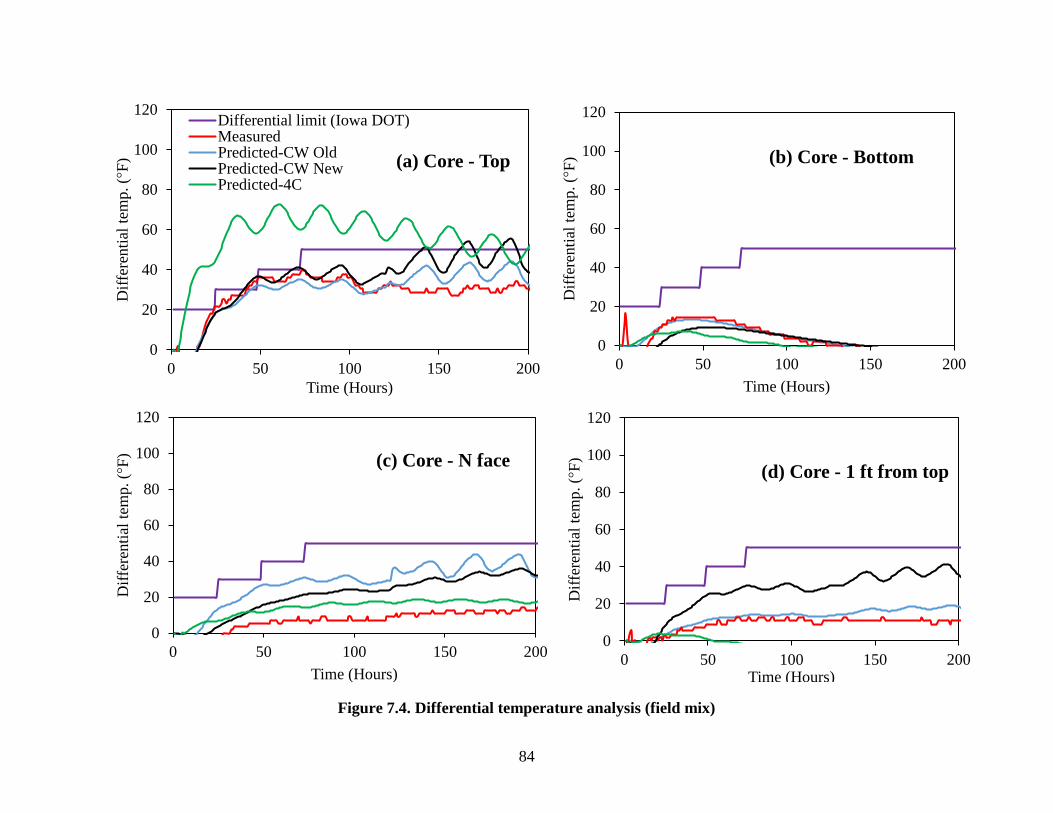
84
Figure 7.4. Differential temperature analysis (field mix)
0
20
40
60
80
100
120
0 50 100 150 200
Dif
fere
nti
al t
emp. (°
F)
Time (Hours)
(a) Core - Top
Differential limit (Iowa DOT)MeasuredPredicted-CW OldPredicted-CW NewPredicted-4C
0
20
40
60
80
100
120
0 50 100 150 200
Dif
fere
nti
al t
emp. (°
F)
Time (Hours)
(b) Core - Bottom
0
20
40
60
80
100
120
0 50 100 150 200
Dif
fere
nti
al t
emp. (°
F)
Time (Hours)
(c) Core - N face
0
20
40
60
80
100
120
0 50 100 150 200
Dif
fere
nti
al t
emp. (°
F)
Time (Hours)
(d) Core - 1 ft from top
85
The time series for maximum temperature differential specified by the Iowa DOT are also
plotted in these charts. The specification states that the differential temperature between the
centroid and a point 2 to 4 in. inside the surface along the shortest line from the centroid to the
nearest surface or top surface of the element shall not exceed 20°F in the first 24 hours, 30°F
between 24–48 hours, 40°F between 48–72 hours, and 50°F after that. The observations from
these charts are as follows:
1. The measured temperature difference, between the core and top of the footing, is within the
Iowa DOT limits for most of the early-age period as shown in Figure 7.4(a). The 4C
predictions of this parameter are very high, probably because the temperature predicted by
4C at the top is lower than that of the measured values. The new ConcreteWorks prediction
of the core and top differential temperature profile is very similar to the measured profile.
Since this is the most critical differential location, its prediction as close as possible to the
actual value will be helpful in developing a TCP.
2. The profile of the temperature difference between the core and bottom sensors is shown in
Figure 7.4(b). The ConcreteWorks predictions are a bit lower than the measured values but
are all within the specification limits.
3. The temperature difference between the core and the center of the face at the shortest
distance from the core (the north face) is also very critical for thermal cracking. The
measured temperature difference for the field project was very well within the specification
limits as shown in Figure 7.4(c). Prediction by all three programs is higher than the measured
values and also within the limits. Considering a factor of safety for important projects,
predictions on a bit higher side could be acceptable.
4. As discussed earlier, the temperature at a location 1 ft from the top was also analyzed. The
differential temperature between the core and this point is shown in Figure 7.4(d). The 4C
predictions of this parameter are lower than the actual value. However, the ConcreteWorks
profile of temperature difference is higher than the actual value.
Maturity
ConcreteWorks has the option of choosing one of the methods amongst Nurse-Saul and
equivalent age for computing the maturity index. The user can select either of the two. However,
due to its simplicity, the Nurse-Saul method is frequently used for construction projects in Iowa
and, for this reason, as well as for this research, this method was used. The coefficients a and b
of the best-fit strength-maturity equation were used as input to the ConcreteWorks program.
Figure 7.5 shows the comparison of the measured and ConcreteWorks predicted values for
maturity presented in terms of a TTF against the age of the concrete.
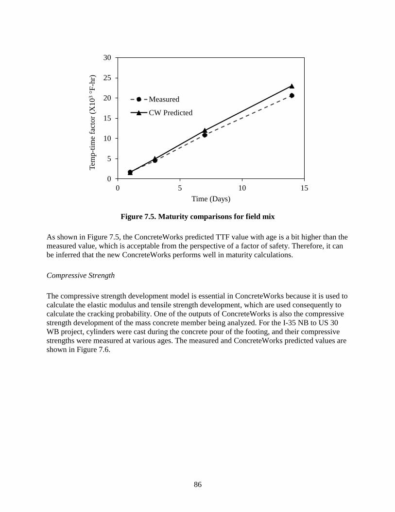
86
Figure 7.5. Maturity comparisons for field mix
As shown in Figure 7.5, the ConcreteWorks predicted TTF value with age is a bit higher than the
measured value, which is acceptable from the perspective of a factor of safety. Therefore, it can
be inferred that the new ConcreteWorks performs well in maturity calculations.
Compressive Strength
The compressive strength development model is essential in ConcreteWorks because it is used to
calculate the elastic modulus and tensile strength development, which are used consequently to
calculate the cracking probability. One of the outputs of ConcreteWorks is also the compressive
strength development of the mass concrete member being analyzed. For the I-35 NB to US 30
WB project, cylinders were cast during the concrete pour of the footing, and their compressive
strengths were measured at various ages. The measured and ConcreteWorks predicted values are
shown in Figure 7.6.
0
5
10
15
20
25
30
0 5 10 15
Tem
p-t
ime
fact
or
(X1
03
°F-h
r)
Time (Days)
Measured
CW Predicted
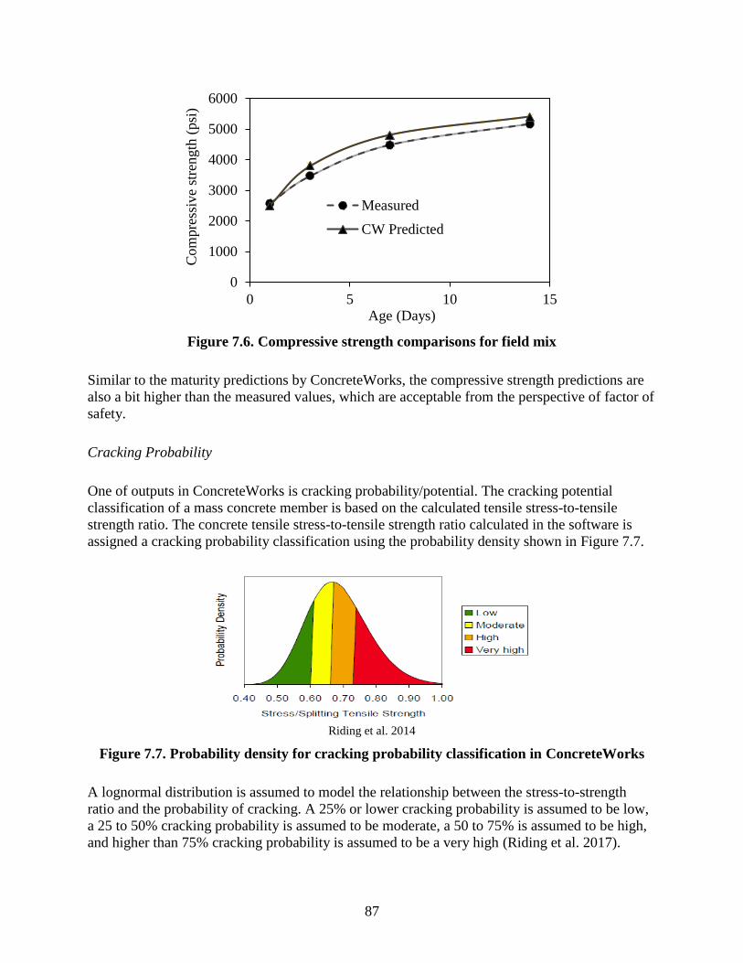
87
Figure 7.6. Compressive strength comparisons for field mix
Similar to the maturity predictions by ConcreteWorks, the compressive strength predictions are
also a bit higher than the measured values, which are acceptable from the perspective of factor of
safety.
Cracking Probability
One of outputs in ConcreteWorks is cracking probability/potential. The cracking potential
classification of a mass concrete member is based on the calculated tensile stress-to-tensile
strength ratio. The concrete tensile stress-to-tensile strength ratio calculated in the software is
assigned a cracking probability classification using the probability density shown in Figure 7.7.
Riding et al. 2014
Figure 7.7. Probability density for cracking probability classification in ConcreteWorks
A lognormal distribution is assumed to model the relationship between the stress-to-strength
ratio and the probability of cracking. A 25% or lower cracking probability is assumed to be low,
a 25 to 50% cracking probability is assumed to be moderate, a 50 to 75% is assumed to be high,
and higher than 75% cracking probability is assumed to be a very high (Riding et al. 2017).
0
1000
2000
3000
4000
5000
6000
0 5 10 15
Com
pre
ssiv
e st
rength
(psi
)
Age (Days)
Measured
CW Predicted
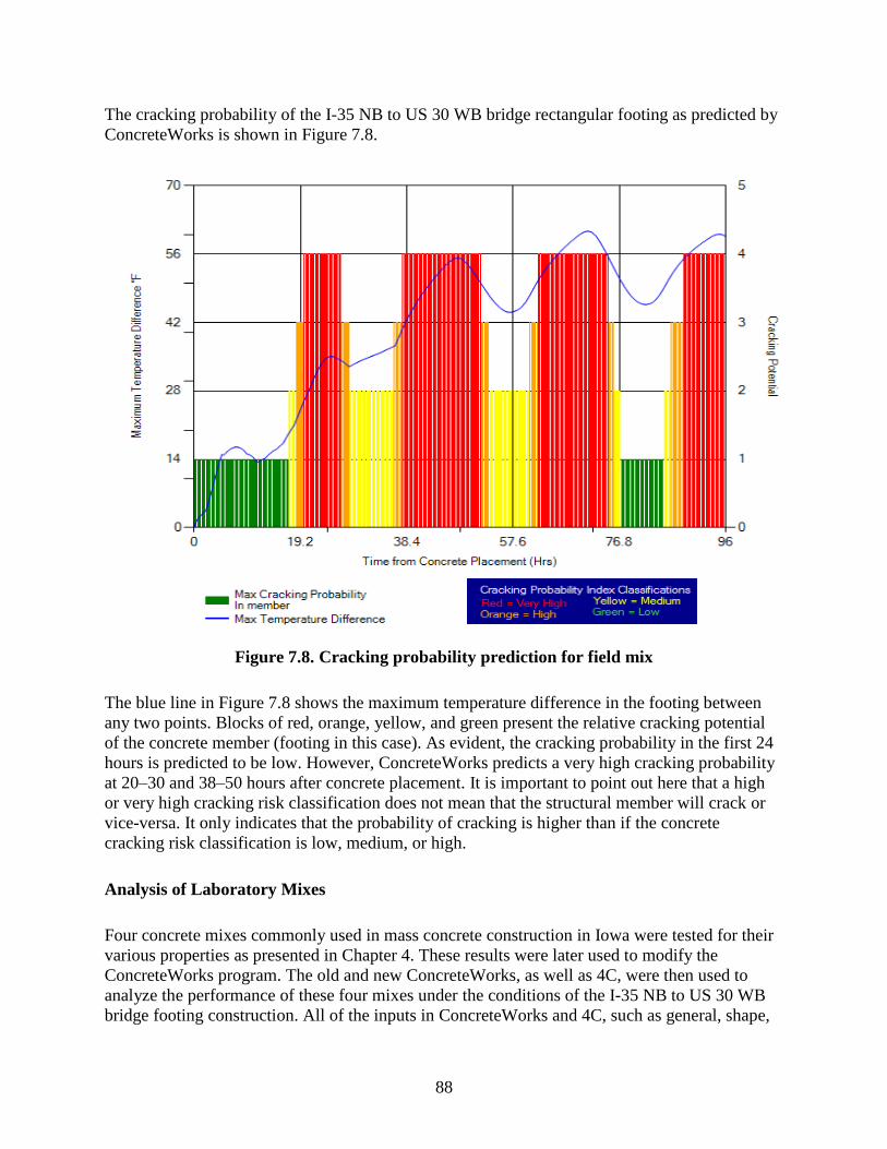
88
The cracking probability of the I-35 NB to US 30 WB bridge rectangular footing as predicted by
ConcreteWorks is shown in Figure 7.8.
Figure 7.8. Cracking probability prediction for field mix
The blue line in Figure 7.8 shows the maximum temperature difference in the footing between
any two points. Blocks of red, orange, yellow, and green present the relative cracking potential
of the concrete member (footing in this case). As evident, the cracking probability in the first 24
hours is predicted to be low. However, ConcreteWorks predicts a very high cracking probability
at 20–30 and 38–50 hours after concrete placement. It is important to point out here that a high
or very high cracking risk classification does not mean that the structural member will crack or
vice-versa. It only indicates that the probability of cracking is higher than if the concrete
cracking risk classification is low, medium, or high.
Analysis of Laboratory Mixes
Four concrete mixes commonly used in mass concrete construction in Iowa were tested for their
various properties as presented in Chapter 4. These results were later used to modify the
ConcreteWorks program. The old and new ConcreteWorks, as well as 4C, were then used to
analyze the performance of these four mixes under the conditions of the I-35 NB to US 30 WB
bridge footing construction. All of the inputs in ConcreteWorks and 4C, such as general, shape,

89
construction, and environmental inputs, were kept the same as those used in the analysis of the
field mix. Figure 7.9 shows the input values for one of the mixes (Mix 1).
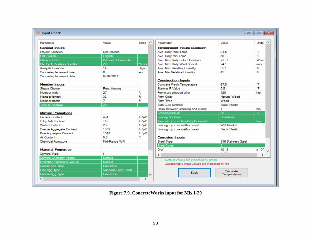
90
Figure 7.9. ConcreteWorks input for Mix I-20
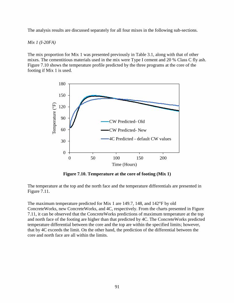
91
The analysis results are discussed separately for all four mixes in the following sub-sections.
Mix 1 (I-20FA)
The mix proportion for Mix 1 was presented previously in Table 3.1, along with that of other
mixes. The cementitious materials used in the mix were Type I cement and 20 % Class C fly ash.
Figure 7.10 shows the temperature profile predicted by the three programs at the core of the
footing if Mix 1 is used.
Figure 7.10. Temperature at the core of footing (Mix 1)
The temperature at the top and the north face and the temperature differentials are presented in
Figure 7.11.
The maximum temperature predicted for Mix 1 are 149.7, 148, and 142°F by old
ConcreteWorks, new ConcreteWorks, and 4C, respectively. From the charts presented in Figure
7.11, it can be observed that the ConcreteWorks predictions of maximum temperature at the top
and north face of the footing are higher than that predicted by 4C. The ConcreteWorks predicted
temperature differential between the core and the top are within the specified limits; however,
that by 4C exceeds the limit. On the other hand, the prediction of the differential between the
core and north face are all within the limits.
0
30
60
90
120
150
180
0 50 100 150 200
Tem
per
ature
(°F
)
Time (Hours)
CW Predicted- Old
CW Predicted- New
4C Predicted - default CW values
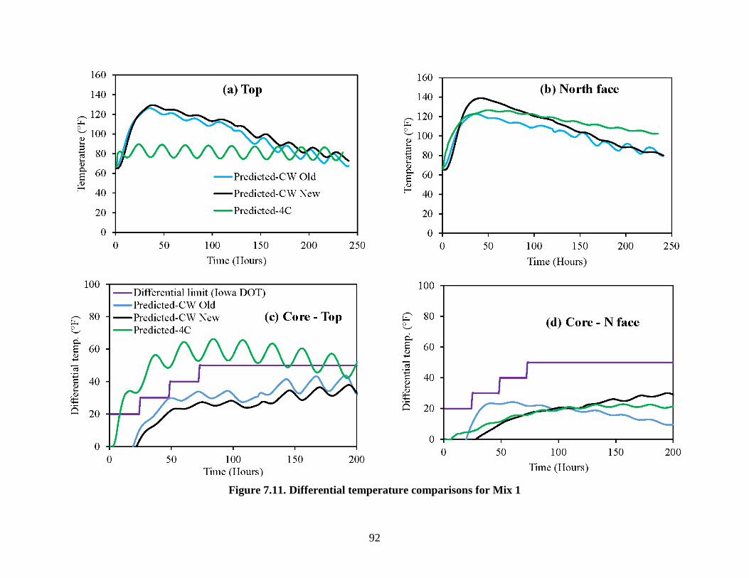
92
Figure 7.11. Differential temperature comparisons for Mix 1
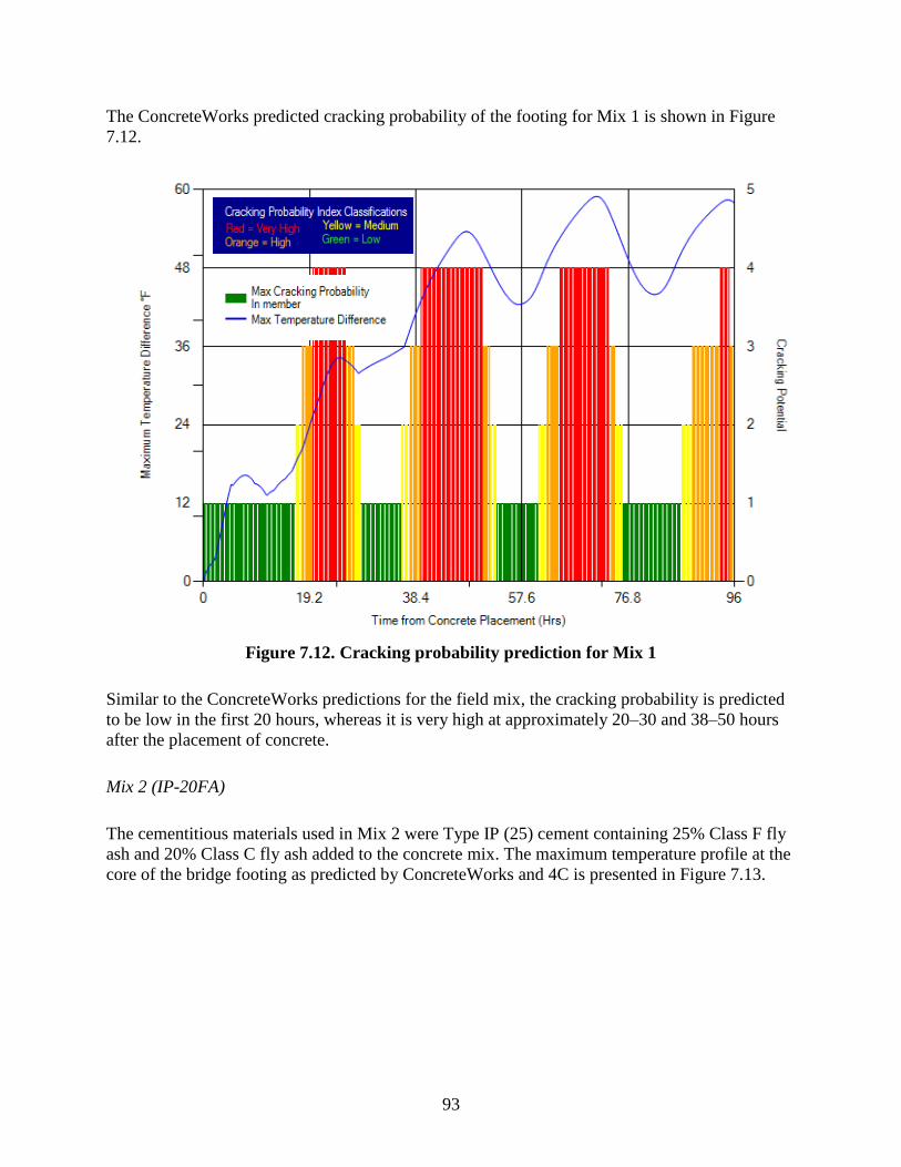
93
The ConcreteWorks predicted cracking probability of the footing for Mix 1 is shown in Figure
7.12.
Figure 7.12. Cracking probability prediction for Mix 1
Similar to the ConcreteWorks predictions for the field mix, the cracking probability is predicted
to be low in the first 20 hours, whereas it is very high at approximately 20–30 and 38–50 hours
after the placement of concrete.
Mix 2 (IP-20FA)
The cementitious materials used in Mix 2 were Type IP (25) cement containing 25% Class F fly
ash and 20% Class C fly ash added to the concrete mix. The maximum temperature profile at the
core of the bridge footing as predicted by ConcreteWorks and 4C is presented in Figure 7.13.
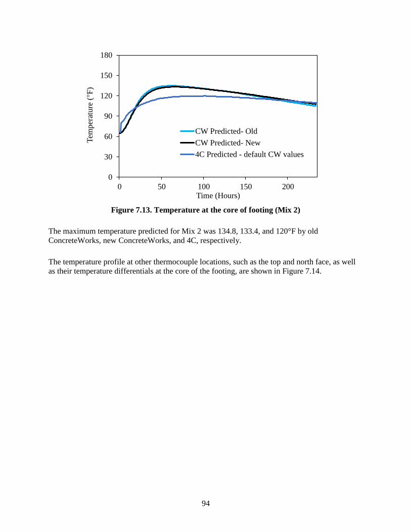
94
Figure 7.13. Temperature at the core of footing (Mix 2)
The maximum temperature predicted for Mix 2 was 134.8, 133.4, and 120°F by old
ConcreteWorks, new ConcreteWorks, and 4C, respectively.
The temperature profile at other thermocouple locations, such as the top and north face, as well
as their temperature differentials at the core of the footing, are shown in Figure 7.14.
0
30
60
90
120
150
180
0 50 100 150 200
Tem
per
ature
(°F
)
Time (Hours)
CW Predicted- Old
CW Predicted- New
4C Predicted - default CW values
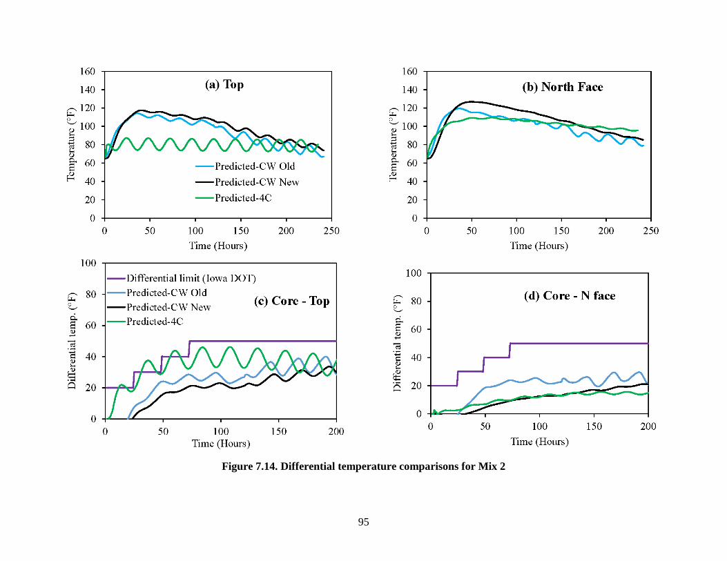
95
Figure 7.14. Differential temperature comparisons for Mix 2
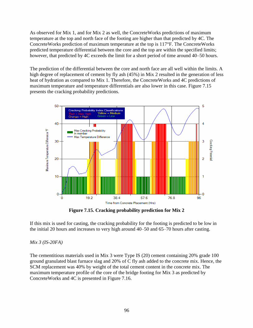
96
As observed for Mix 1, and for Mix 2 as well, the ConcreteWorks predictions of maximum
temperature at the top and north face of the footing are higher than that predicted by 4C. The
ConcreteWorks prediction of maximum temperature at the top is 117°F. The ConcreteWorks
predicted temperature differential between the core and the top are within the specified limits;
however, that predicted by 4C exceeds the limit for a short period of time around 40–50 hours.
The prediction of the differential between the core and north face are all well within the limits. A
high degree of replacement of cement by fly ash (45%) in Mix 2 resulted in the generation of less
heat of hydration as compared to Mix 1. Therefore, the ConcreteWorks and 4C predictions of
maximum temperature and temperature differentials are also lower in this case. Figure 7.15
presents the cracking probability predictions.
Figure 7.15. Cracking probability prediction for Mix 2
If this mix is used for casting, the cracking probability for the footing is predicted to be low in
the initial 20 hours and increases to very high around 40–50 and 65–70 hours after casting.
Mix 3 (IS-20FA)
The cementitious materials used in Mix 3 were Type IS (20) cement containing 20% grade 100
ground granulated blast furnace slag and 20% of C fly ash added to the concrete mix. Hence, the
SCM replacement was 40% by weight of the total cement content in the concrete mix. The
maximum temperature profile of the core of the bridge footing for Mix 3 as predicted by
ConcreteWorks and 4C is presented in Figure 7.16.
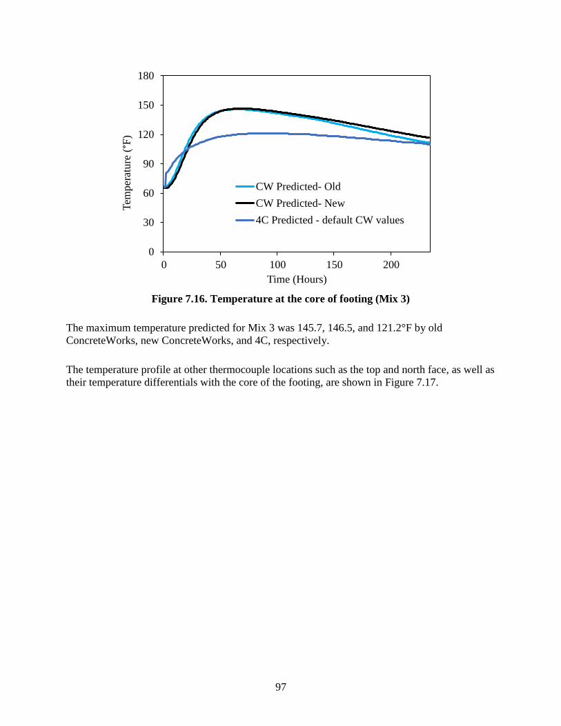
97
Figure 7.16. Temperature at the core of footing (Mix 3)
The maximum temperature predicted for Mix 3 was 145.7, 146.5, and 121.2°F by old
ConcreteWorks, new ConcreteWorks, and 4C, respectively.
The temperature profile at other thermocouple locations such as the top and north face, as well as
their temperature differentials with the core of the footing, are shown in Figure 7.17.
0
30
60
90
120
150
180
0 50 100 150 200
Tem
per
ature
(°F
)
Time (Hours)
CW Predicted- Old
CW Predicted- New
4C Predicted - default CW values
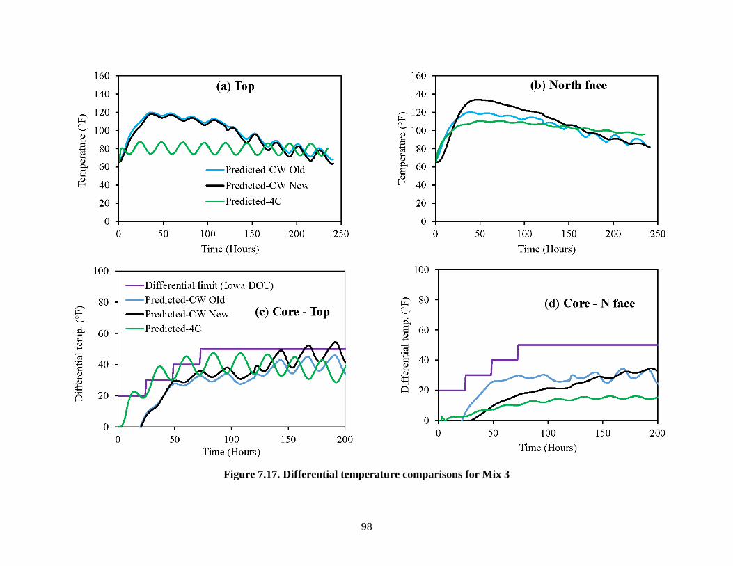
98
Figure 7.17. Differential temperature comparisons for Mix 3
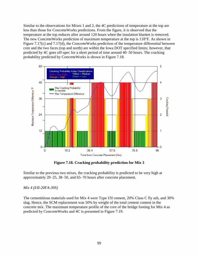
99
Similar to the observations for Mixes 1 and 2, the 4C predictions of temperature at the top are
less than those for ConcreteWorks predictions. From the figure, it is observed that the
temperature at the top reduces after around 120 hours when the insulation blanket is removed.
The new ConcreteWorks prediction of maximum temperature at the top is 118°F. As shown in
Figure 7.17(c) and 7.17(d), the ConcreteWorks prediction of the temperature differential between
core and the two faces (top and north) are within the Iowa DOT specified limits; however, that
predicted by 4C goes off-spec for a short period of time around 40–50 hours. The cracking
probability predicted by ConcreteWorks is shown in Figure 7.18.
Figure 7.18. Cracking probability prediction for Mix 3
Similar to the previous two mixes, the cracking probability is predicted to be very high at
approximately 20–25, 38–50, and 65–70 hours after concrete placement.
Mix 4 (I/II-20FA-30S)
The cementitious materials used for Mix 4 were Type I/II cement, 20% Class C fly ash, and 30%
slag. Hence, the SCM replacement was 50% by weight of the total cement content in the
concrete mix. The maximum temperature profile of the core of the bridge footing for Mix 4 as
predicted by ConcreteWorks and 4C is presented in Figure 7.19.
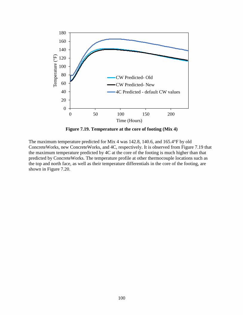
100
Figure 7.19. Temperature at the core of footing (Mix 4)
The maximum temperature predicted for Mix 4 was 142.8, 140.6, and 165.4°F by old
ConcreteWorks, new ConcreteWorks, and 4C, respectively. It is observed from Figure 7.19 that
the maximum temperature predicted by 4C at the core of the footing is much higher than that
predicted by ConcreteWorks. The temperature profile at other thermocouple locations such as
the top and north face, as well as their temperature differentials in the core of the footing, are
shown in Figure 7.20.
0
20
40
60
80
100
120
140
160
180
0 50 100 150 200
Tem
per
ature
(°F
)
Time (Hours)
CW Predicted- Old
CW Predicted- New
4C Predicted - default CW values
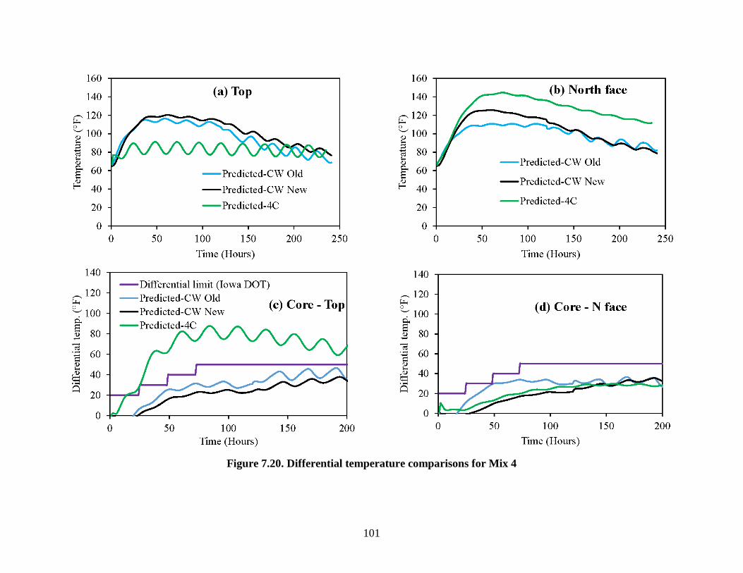
101
Figure 7.20. Differential temperature comparisons for Mix 4
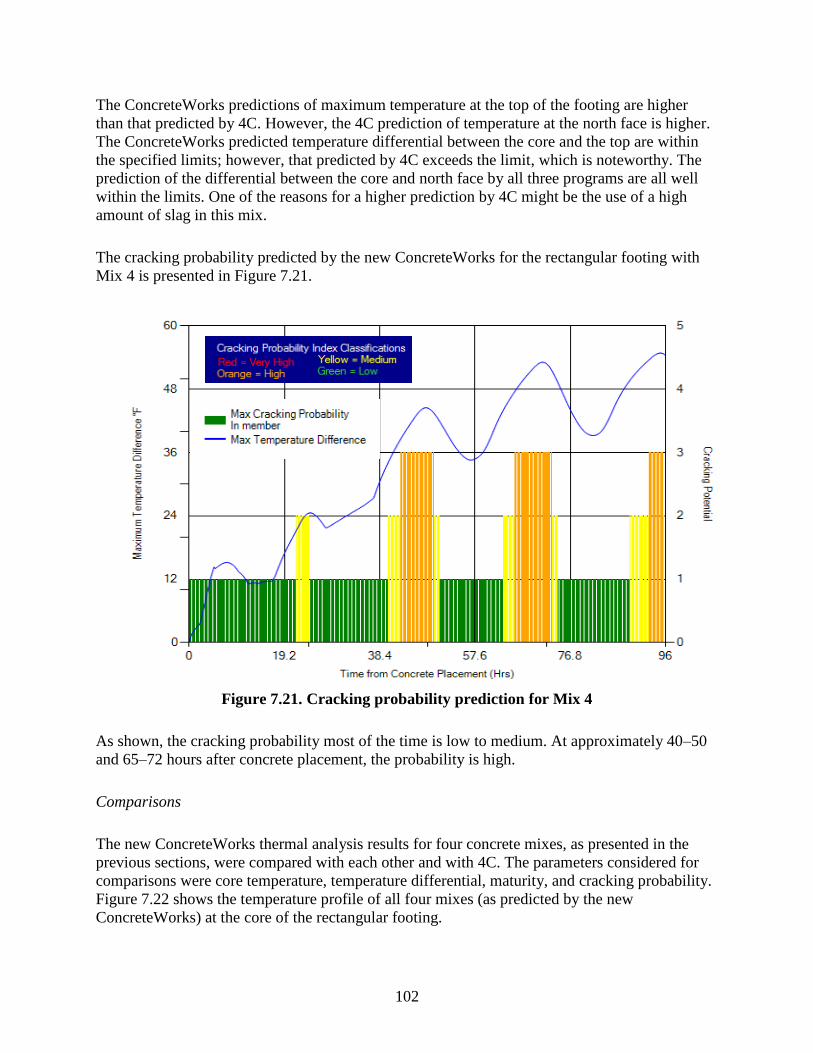
102
The ConcreteWorks predictions of maximum temperature at the top of the footing are higher
than that predicted by 4C. However, the 4C prediction of temperature at the north face is higher.
The ConcreteWorks predicted temperature differential between the core and the top are within
the specified limits; however, that predicted by 4C exceeds the limit, which is noteworthy. The
prediction of the differential between the core and north face by all three programs are all well
within the limits. One of the reasons for a higher prediction by 4C might be the use of a high
amount of slag in this mix.
The cracking probability predicted by the new ConcreteWorks for the rectangular footing with
Mix 4 is presented in Figure 7.21.
Figure 7.21. Cracking probability prediction for Mix 4
As shown, the cracking probability most of the time is low to medium. At approximately 40–50
and 65–72 hours after concrete placement, the probability is high.
Comparisons
The new ConcreteWorks thermal analysis results for four concrete mixes, as presented in the
previous sections, were compared with each other and with 4C. The parameters considered for
comparisons were core temperature, temperature differential, maturity, and cracking probability.
Figure 7.22 shows the temperature profile of all four mixes (as predicted by the new
ConcreteWorks) at the core of the rectangular footing.
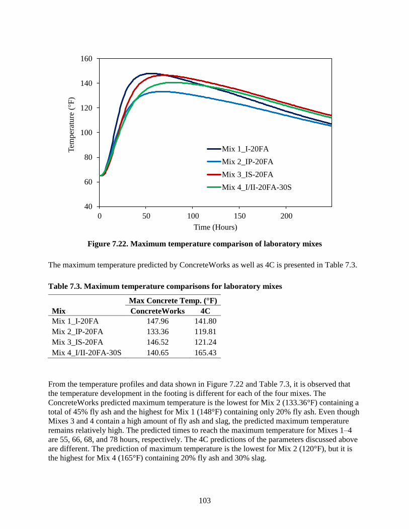
103
Figure 7.22. Maximum temperature comparison of laboratory mixes
The maximum temperature predicted by ConcreteWorks as well as 4C is presented in Table 7.3.
Table 7.3. Maximum temperature comparisons for laboratory mixes
Mix
Max Concrete Temp. (°F)
ConcreteWorks 4C
Mix 1_I-20FA 147.96 141.80
Mix 2_IP-20FA 133.36 119.81
Mix 3_IS-20FA 146.52 121.24
Mix 4_I/II-20FA-30S 140.65 165.43
From the temperature profiles and data shown in Figure 7.22 and Table 7.3, it is observed that
the temperature development in the footing is different for each of the four mixes. The
ConcreteWorks predicted maximum temperature is the lowest for Mix 2 (133.36°F) containing a
total of 45% fly ash and the highest for Mix 1 (148°F) containing only 20% fly ash. Even though
Mixes 3 and 4 contain a high amount of fly ash and slag, the predicted maximum temperature
remains relatively high. The predicted times to reach the maximum temperature for Mixes 1–4
are 55, 66, 68, and 78 hours, respectively. The 4C predictions of the parameters discussed above
are different. The prediction of maximum temperature is the lowest for Mix 2 (120°F), but it is
the highest for Mix 4 (165°F) containing 20% fly ash and 30% slag.
40
60
80
100
120
140
160
0 50 100 150 200
Tem
per
ature
(°F
)
Time (Hours)
Mix 1_I-20FA
Mix 2_IP-20FA
Mix 3_IS-20FA
Mix 4_I/II-20FA-30S
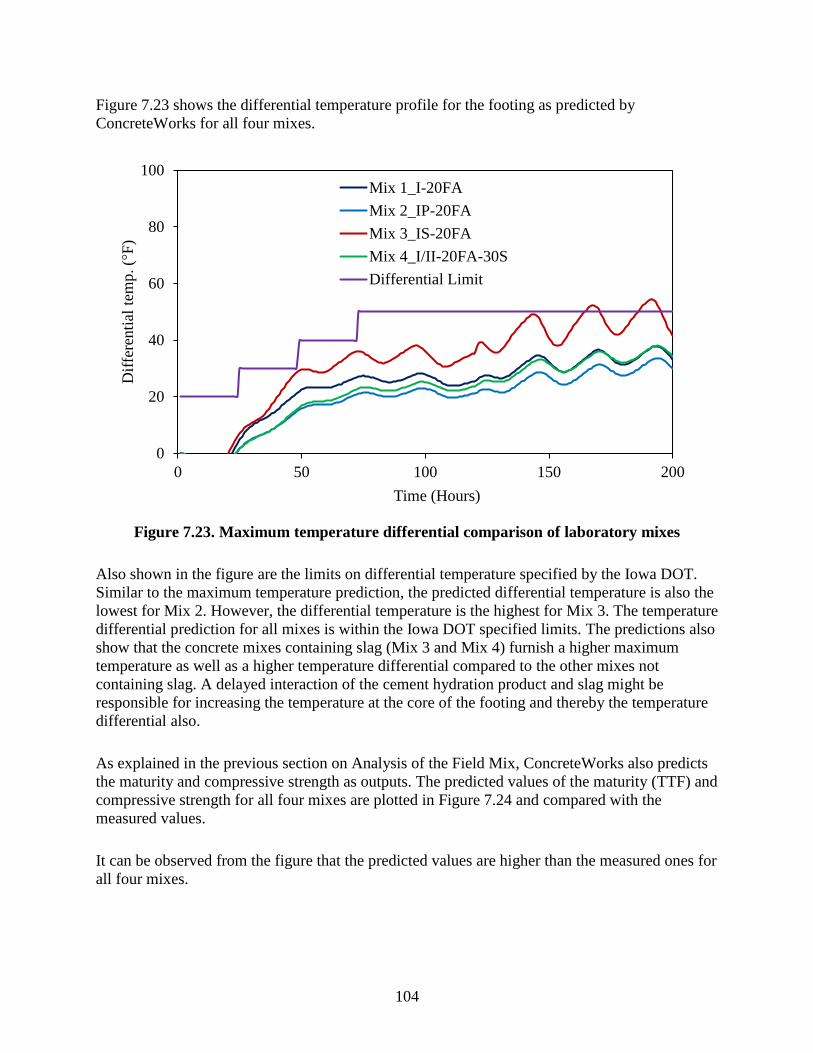
104
Figure 7.23 shows the differential temperature profile for the footing as predicted by
ConcreteWorks for all four mixes.
Figure 7.23. Maximum temperature differential comparison of laboratory mixes
Also shown in the figure are the limits on differential temperature specified by the Iowa DOT.
Similar to the maximum temperature prediction, the predicted differential temperature is also the
lowest for Mix 2. However, the differential temperature is the highest for Mix 3. The temperature
differential prediction for all mixes is within the Iowa DOT specified limits. The predictions also
show that the concrete mixes containing slag (Mix 3 and Mix 4) furnish a higher maximum
temperature as well as a higher temperature differential compared to the other mixes not
containing slag. A delayed interaction of the cement hydration product and slag might be
responsible for increasing the temperature at the core of the footing and thereby the temperature
differential also.
As explained in the previous section on Analysis of the Field Mix, ConcreteWorks also predicts
the maturity and compressive strength as outputs. The predicted values of the maturity (TTF) and
compressive strength for all four mixes are plotted in Figure 7.24 and compared with the
measured values.
It can be observed from the figure that the predicted values are higher than the measured ones for
all four mixes.
0
20
40
60
80
100
0 50 100 150 200
Dif
fere
nti
al t
emp. (°
F)
Time (Hours)
Mix 1_I-20FA
Mix 2_IP-20FA
Mix 3_IS-20FA
Mix 4_I/II-20FA-30S
Differential Limit
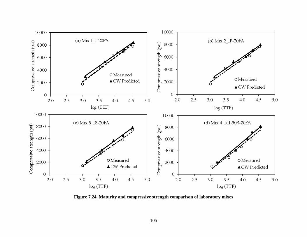
105
Figure 7.24. Maturity and compressive strength comparison of laboratory mixes
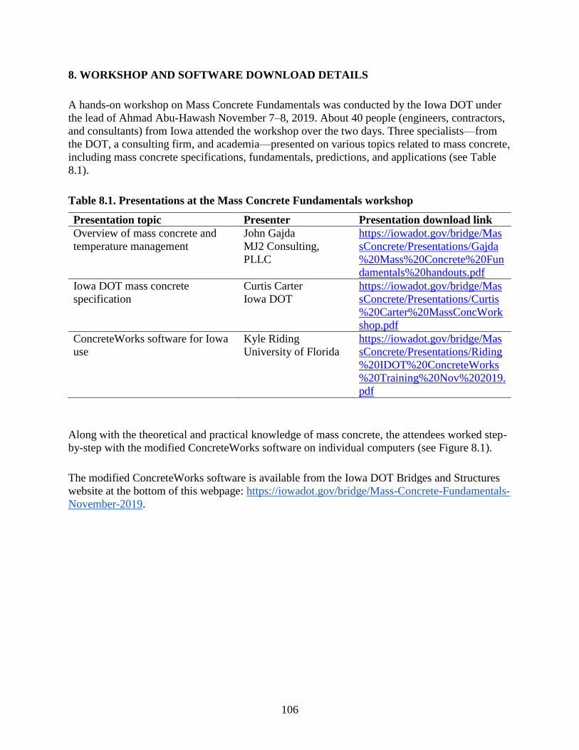
106
8. WORKSHOP AND SOFTWARE DOWNLOAD DETAILS
A hands-on workshop on Mass Concrete Fundamentals was conducted by the Iowa DOT under
the lead of Ahmad Abu-Hawash November 7–8, 2019. About 40 people (engineers, contractors,
and consultants) from Iowa attended the workshop over the two days. Three specialists—from
the DOT, a consulting firm, and academia—presented on various topics related to mass concrete,
including mass concrete specifications, fundamentals, predictions, and applications (see Table
8.1).
Table 8.1. Presentations at the Mass Concrete Fundamentals workshop
Presentation topic Presenter Presentation download link
Overview of mass concrete and
temperature management
John Gajda
MJ2 Consulting,
PLLC
https://iowadot.gov/bridge/Mas
sConcrete/Presentations/Gajda
%20Mass%20Concrete%20Fun
damentals%20handouts.pdf
Iowa DOT mass concrete
specification
Curtis Carter
Iowa DOT
https://iowadot.gov/bridge/Mas
sConcrete/Presentations/Curtis
%20Carter%20MassConcWork
shop.pdf
ConcreteWorks software for Iowa
use
Kyle Riding
University of Florida
https://iowadot.gov/bridge/Mas
sConcrete/Presentations/Riding
%20IDOT%20ConcreteWorks
%20Training%20Nov%202019.
Along with the theoretical and practical knowledge of mass concrete, the attendees worked step-
by-step with the modified ConcreteWorks software on individual computers (see Figure 8.1).
The modified ConcreteWorks software is available from the Iowa DOT Bridges and Structures
website at the bottom of this webpage: https://iowadot.gov/bridge/Mass-Concrete-Fundamentals-
November-2019.
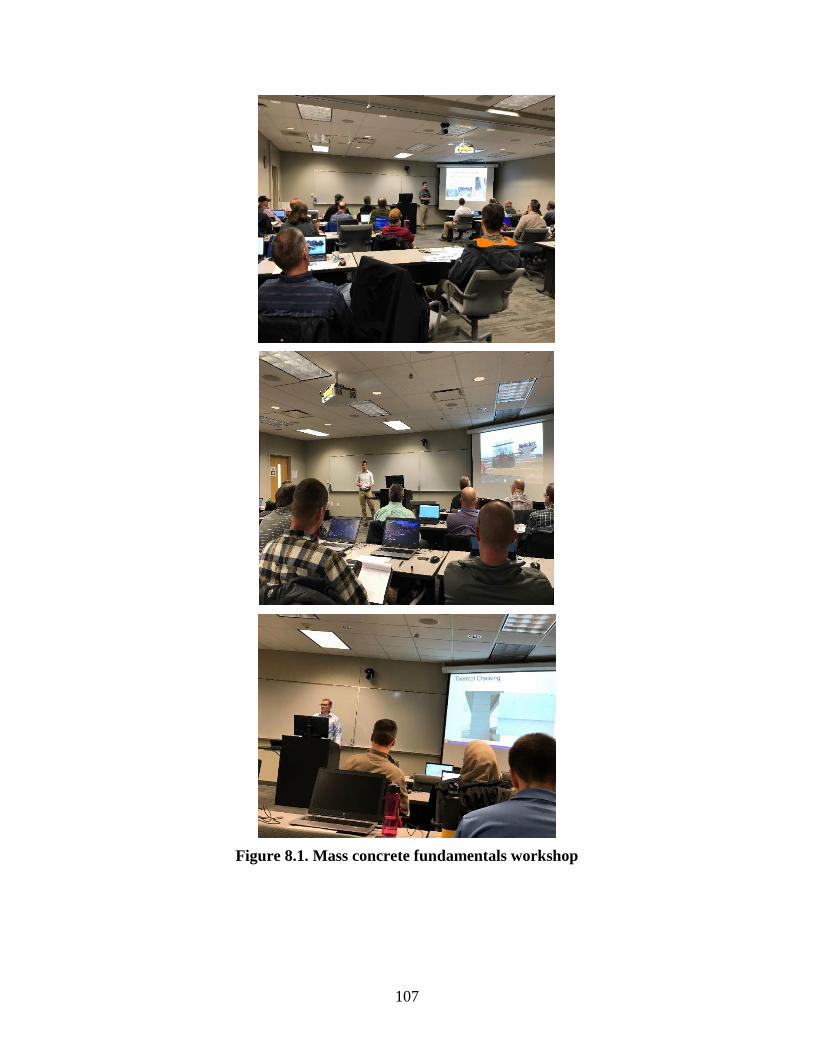
107
Figure 8.1. Mass concrete fundamentals workshop
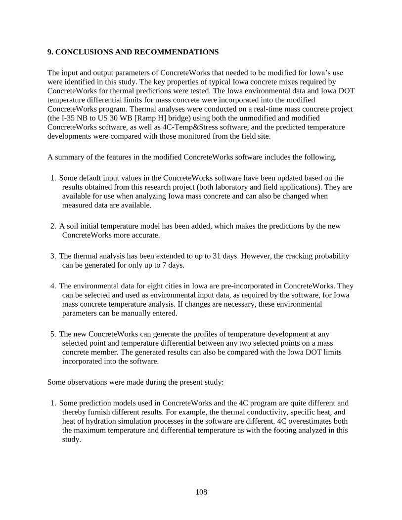
108
9. CONCLUSIONS AND RECOMMENDATIONS
The input and output parameters of ConcreteWorks that needed to be modified for Iowa’s use
were identified in this study. The key properties of typical Iowa concrete mixes required by
ConcreteWorks for thermal predictions were tested. The Iowa environmental data and Iowa DOT
temperature differential limits for mass concrete were incorporated into the modified
ConcreteWorks program. Thermal analyses were conducted on a real-time mass concrete project
(the I-35 NB to US 30 WB [Ramp H] bridge) using both the unmodified and modified
ConcreteWorks software, as well as 4C-Temp&Stress software, and the predicted temperature
developments were compared with those monitored from the field site.
A summary of the features in the modified ConcreteWorks software includes the following.
1. Some default input values in the ConcreteWorks software have been updated based on the
results obtained from this research project (both laboratory and field applications). They are
available for use when analyzing Iowa mass concrete and can also be changed when
measured data are available.
2. A soil initial temperature model has been added, which makes the predictions by the new
ConcreteWorks more accurate.
3. The thermal analysis has been extended to up to 31 days. However, the cracking probability
can be generated for only up to 7 days.
4. The environmental data for eight cities in Iowa are pre-incorporated in ConcreteWorks. They
can be selected and used as environmental input data, as required by the software, for Iowa
mass concrete temperature analysis. If changes are necessary, these environmental
parameters can be manually entered.
5. The new ConcreteWorks can generate the profiles of temperature development at any
selected point and temperature differential between any two selected points on a mass
concrete member. The generated results can also be compared with the Iowa DOT limits
incorporated into the software.
Some observations were made during the present study:
1. Some prediction models used in ConcreteWorks and the 4C program are quite different and
thereby furnish different results. For example, the thermal conductivity, specific heat, and
heat of hydration simulation processes in the software are different. 4C overestimates both
the maximum temperature and differential temperature as with the footing analyzed in this
study.
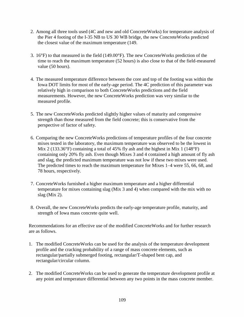
109
2. Among all three tools used (4C and new and old ConcreteWorks) for temperature analysis of
the Pier 4 footing of the I-35 NB to US 30 WB bridge, the new ConcreteWorks predicted
the closest value of the maximum temperature (149.
3. 16°F) to that measured in the field (149.00°F). The new ConcreteWorks prediction of the
time to reach the maximum temperature (52 hours) is also close to that of the field-measured
value (50 hours).
4. The measured temperature difference between the core and top of the footing was within the
Iowa DOT limits for most of the early-age period. The 4C prediction of this parameter was
relatively high in comparison to both ConcreteWorks predictions and the field
measurements. However, the new ConcreteWorks prediction was very similar to the
measured profile.
5. The new ConcreteWorks predicted slightly higher values of maturity and compressive
strength than those measured from the field concrete; this is conservative from the
perspective of factor of safety.
6. Comparing the new ConcreteWorks predictions of temperature profiles of the four concrete
mixes tested in the laboratory, the maximum temperature was observed to be the lowest in
Mix 2 (133.36°F) containing a total of 45% fly ash and the highest in Mix 1 (148°F)
containing only 20% fly ash. Even though Mixes 3 and 4 contained a high amount of fly ash
and slag, the predicted maximum temperature was not low if these two mixes were used.
The predicted times to reach the maximum temperature for Mixes 1–4 were 55, 66, 68, and
78 hours, respectively.
7. ConcreteWorks furnished a higher maximum temperature and a higher differential
temperature for mixes containing slag (Mix 3 and 4) when compared with the mix with no
slag (Mix 2).
8. Overall, the new ConcreteWorks predicts the early-age temperature profile, maturity, and
strength of Iowa mass concrete quite well.
Recommendations for an effective use of the modified ConcreteWorks and for further research
are as follows.
1. The modified ConcreteWorks can be used for the analysis of the temperature development
profile and the cracking probability of a range of mass concrete elements, such as
rectangular/partially submerged footing, rectangular/T-shaped bent cap, and
rectangular/circular column.
2. The modified ConcreteWorks can be used to generate the temperature development profile at
any point and temperature differential between any two points in the mass concrete member.
110
The generated results can also be compared with the Iowa DOT temperature differential
limits incorporated in the software.
3. The weblink for the ConcreteWorks workshop conducted during this project can serve as a
resource for engineers that are interested in learning how to use the softward. The
ConcreteWorks Operator’s Manual developed during this project can also serve as a
reference to help users input data and interpret results properly. Additional workshops/short
courses can be conducted to teach potential users how to use the manual and further
understand the software.
4. Some of the default values (material properties, hydration parameters, formwork insulation,
etc.) can be further modified if the measured data are available. It was observed in this study
that compared to portland cement and fly ash containing mixes, the concrete mixes
containing slag might exhibit a higher adiabatic temperature rise if used in mass concrete
construction. Considering the interaction of slag and portland cement, further research can be
performed to investigate the heat generation in slag-containing concrete mixes. A new model
can also be developed to predict the temperature development profile of mass concrete
members where such mixes are used. In addition, limestone cement is increasingly used in
Iowa but not included in the present study. Investigation into the thermal behavior of mass
concrete containing limestone cement may be necessary in the very near future.
5. In a bridge foundation design and construction, cofferdams are built to form watertight
enclosures surrounding excavations. These enclosures normally consist of sheet piling driven
around the perimeter of the excavation. A concrete seal coat is placed within the sheet piling,
and the bridge footing is then built on the seal coat slab. A concern was raised in the present
study on how the temperature profile of the seal coat slab can affect the early-age
temperature development in the footing placed above it. Currently, the ConcreteWorks
software doesn’t have the capability to predict the concrete temperature of seal coat slabs.
This demands further study.
111
REFERENCES
ACI Committee 207. 2006. Guide to Mass Concrete. ACI 207.1R-05. American Concrete
Institute, Farmington Hills, MI.
ASTM C177. 2004. Standard Test Method for Steady-State Heat Flux Measurements and
Thermal Transmission Properties by Means of the Guarded-Hot-Plate Apparatus. ASTM
International, West Conshohocken, PA.
ASTM C192. 2016. Standard Practice for Making and Curing Concrete Test Specimens in the
Laboratory. ASTM International, West Conshohocken, PA.
Bai, H. 2013. Validation of Cylindrical Pavement Specimen Thermal Conductivity Protocol. MS
thesis. Iowa State University, Ames, IA.
Barber, E. S. 1957. Calculation of Maximum Pavement Temperatures from Weather Reports.
Highway Research Board Bulletin, No. 168, pp. 1–8.
Carlson, J. D., R. Bhardwaj, P. E. Phelan, K. E. Kaloush, and J. S. Golden. 2010. Determining
Thermal Conductivity of Paving Materials Using Cylindrical Sample Geometry. Journal
of Materials in Civil Engineering, Vol. 22, No. 2, pp. 186–95.
De Schutter, G. and L Taerwe. 1996. Degree of Hydration-Based Description of Mechanical
Properties of Early Age Concrete. Materials and Structures, Vol. 29, No. 335.
Emanuel, J. H. and J. L. Hulsey. 1977. Prediction of the Thermal Coefficient of Expansion of
Concrete. ACI Journal Proceedings, Vol. 74, No. 4, pp. 149–155.
Folliard, K. 2010. 3. Heat of Hydration and Thermal Stress Anlalysis. Training Materials
presentation slides. University of Texas Concrete Durability Center, Center for
Transportation Research, University of Texas at Austin, TX.
https://library.ctr.utexas.edu/digitized/products/5-4563-01-P1_PDFsOnly.zip.
Meeks, C. and K. Folliard. 2013. ConcreteWorks Implementation: Final Report. Center for
Transportation Research, University of Texas at Austin, TX.
Poole, J. L. 2007. Modeling Temperature Sensitivity and Heat Evolution of Concrete. PhD
dissertation. University of Texas at Austin, TX.
Poole, J. L., K. A. Riding, K. J. Folliard, M. C. G. Juenger, and A. K Schindler. 2007. Methods
for Calculating Activation Energy for Portland Cement. Materials Journal, Vol. 104,
No. 1, pp. 303–311.
Riding, K. A. 2007. Early Age Concrete Thermal Stress Measurement and Modeling. PhD
dissertation. University of Texas at Austin, Austin, TX.
Riding, K. A., J. L. Poole, A. K. Schindler, M. C. G. Juenger, and K. J. Folliard. 2006.
Evaluation of Temperature Prediction Methods for Mass Concrete Members. Materials
Journal, Vol. 103, No. 5, pp. 357–65.
Riding, K. A., J. L. Poole, K. J. Folliard, M. C. G. Juenger, and A. K. Schindler. 2011. New
Model for Estimating Apparent Activation Energy of Cementitious Systems. Materials
Journal, Vol. 108, No. 5, pp. 550–557.
Riding, K. A., J. L. Poole, A. K. Schindler, M. C. G. Juenger, and K. J. Folliard. 2014. Statistical
Determination of Cracking Probability for Mass Concrete. Journal of Materials in Civil
Engineering, Vol. 26, No. 9, pp. 1–13.
Riding, K., A. Schindler, P. Pesek, T. Drimalas, and K. Folliard. 2017. ConcreteWorks V3
Training/User Manual (P1) ConcreteWorks Software (P2). Center for Transportation
Research, University of Texas at Austin, Austin, TX.

112
Schindler, A. K. 2002. Concrete Hydration, Temperature Development, and Setting at Early-
Ages. PhD dissertation. University of Texas at Austin, TX.
Schindler, A. K. 2004. Effect of Temperature on Hydration of Cementitious Materials. Materials
Journal, Vol. 101, No. 1, pp. 72–81.
Shaw, J. J., C. T. Jahren, K. Wang, and J. L. Li. 2011. Iowa Mass Concrete for Bridge
Foundation Study – Phase I. Institute for Transportation, Iowa State University, Ames,
IA. https://intrans.iastate.edu/app/uploads/2018/03/mass_concrete_i_w_cvr.pdf.
Shaw, J. J., C. T. Jahren, K. Wang, and J. L. Li. 2014. Iowa Mass Concrete for Bridge
Foundation Study – Phase II. Institute for Transportation, Iowa State University, Ames,
IA. https://intrans.iastate.edu/app/uploads/2018/03/mass_concrete_ii_w_cvr2.pdf.
Van Breugel, K. 1998. Prediction of Temperature in Hardening Concrete. In Prevention of
Thermal Cracking in Concrete at Early Ages. RILEM Technical Committee 119, E & Fn
Spon, London, pp. 51–74.
Viviani, M. 2005. Monitoring and Modelling of Construction Materials During Hardening. PhD
dissertation. Swiss Federal Institute of Technology, Zürich, Switzerland.

113
APPENDIX A. CALIBRATION OF ISOTHERMAL CALORIMETER
Steps of the calibration procedure are as follows:
1. Using a multimeter, resistance R of the calibration inserts (1500 Ohm) are checked.
2. To initiate calibration, the environmental chamber is first set at the desired temperatures—10,
20, 30, and 40°C—one by one.
3. After the desired temperature is obtained, the baseline is recorded for a minimum of 24
hours. The average reading for each cell is the baseline, V0.
4. The calibration insert is inserted into cell 1 with connections to a power source but no power
applied, and the lid of the calorimeter chamber is closed completely.
5. A standard voltage Vref of 15 V is applied over the calibration insert in one of the cells and
output voltages measured in the calorimeter are recorded.
6. When the output voltage stays constant, usually after 4 hours, the average of the constant
voltages is taken as V1.
7. Standard voltage is turned off and the calorimeter is allowed to stabilize.
8. The above steps are repeated for all other cells and at other temperatures.
9. The calibration factor is then calculated as follows.
𝑃 = 𝑉𝑟𝑒𝑓
2
𝑅
𝐶𝐹 = 𝑃
𝑉1−𝑉0
Table A.1 presents the calculated values of calibration factors used in this study for eight
channels of the calorimeter at 10, 20, 30, and 40°C.
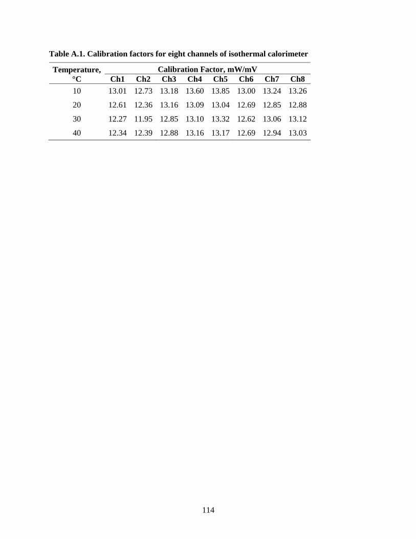
114
Table A.1. Calibration factors for eight channels of isothermal calorimeter
Temperature,
°C
Calibration Factor, mW/mV
Ch1 Ch2 Ch3 Ch4 Ch5 Ch6 Ch7 Ch8
10 13.01 12.73 13.18 13.60 13.85 13.00 13.24 13.26
20 12.61 12.36 13.16 13.09 13.04 12.69 12.85 12.88
30 12.27 11.95 12.85 13.10 13.32 12.62 13.06 13.12
40 12.34 12.39 12.88 13.16 13.17 12.69 12.94 13.03
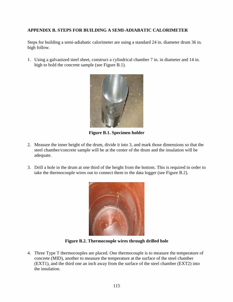
115
APPENDIX B. STEPS FOR BUILDING A SEMI-ADIABATIC CALORIMETER
Steps for building a semi-adiabatic calorimeter are using a standard 24 in. diameter drum 36 in.
high follow.
1. Using a galvanized steel sheet, construct a cylindrical chamber 7 in. in diameter and 14 in.
high to hold the concrete sample (see Figure B.1).
Figure B.1. Specimen holder
2. Measure the inner height of the drum, divide it into 3, and mark those dimensions so that the
steel chamber/concrete sample will be at the center of the drum and the insulation will be
adequate.
3. Drill a hole in the drum at one third of the height from the bottom. This is required in order to
take the thermocouple wires out to connect them to the data logger (see Figure B.2).
Figure B.2. Thermocouple wires through drilled hole
4. Three Type T thermocouples are placed. One thermocouple is to measure the temperature of
concrete (MID), another to measure the temperature at the surface of the steel chamber
(EXT1), and the third one an inch away from the surface of the steel chamber (EXT2) into
the insulation.
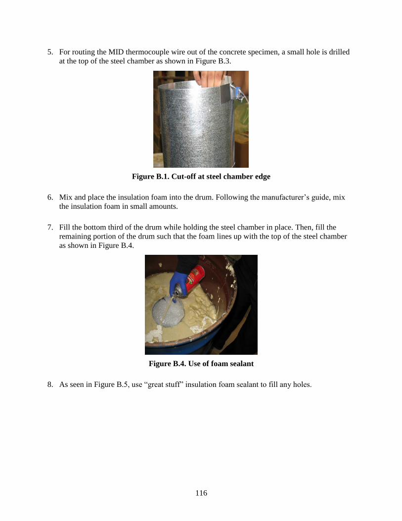
116
5. For routing the MID thermocouple wire out of the concrete specimen, a small hole is drilled
at the top of the steel chamber as shown in Figure B.3.
Figure B.1. Cut-off at steel chamber edge
6. Mix and place the insulation foam into the drum. Following the manufacturer’s guide, mix
the insulation foam in small amounts.
7. Fill the bottom third of the drum while holding the steel chamber in place. Then, fill the
remaining portion of the drum such that the foam lines up with the top of the steel chamber
as shown in Figure B.4.
Figure B.4. Use of foam sealant
8. As seen in Figure B.5, use “great stuff” insulation foam sealant to fill any holes.
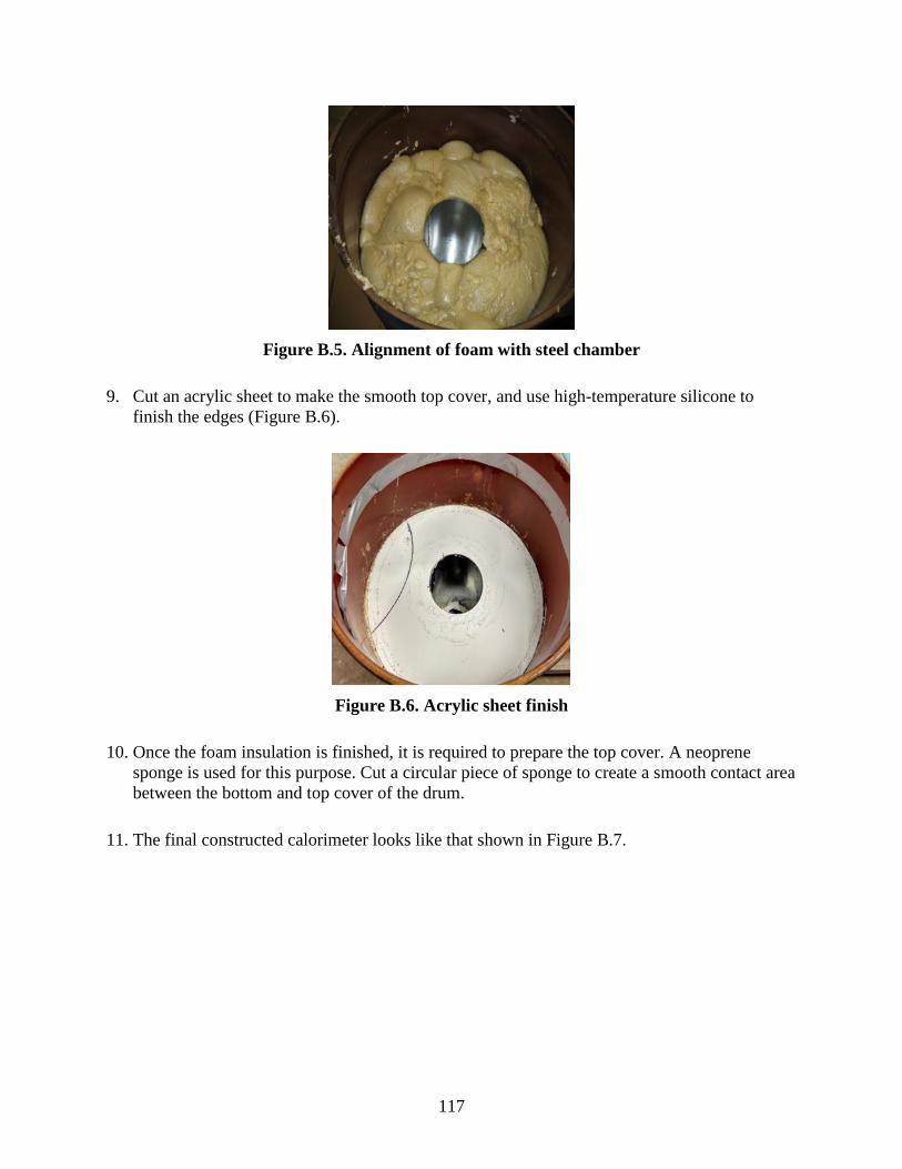
117
Figure B.5. Alignment of foam with steel chamber
9. Cut an acrylic sheet to make the smooth top cover, and use high-temperature silicone to
finish the edges (Figure B.6).
Figure B.6. Acrylic sheet finish
10. Once the foam insulation is finished, it is required to prepare the top cover. A neoprene
sponge is used for this purpose. Cut a circular piece of sponge to create a smooth contact area
between the bottom and top cover of the drum.
11. The final constructed calorimeter looks like that shown in Figure B.7.
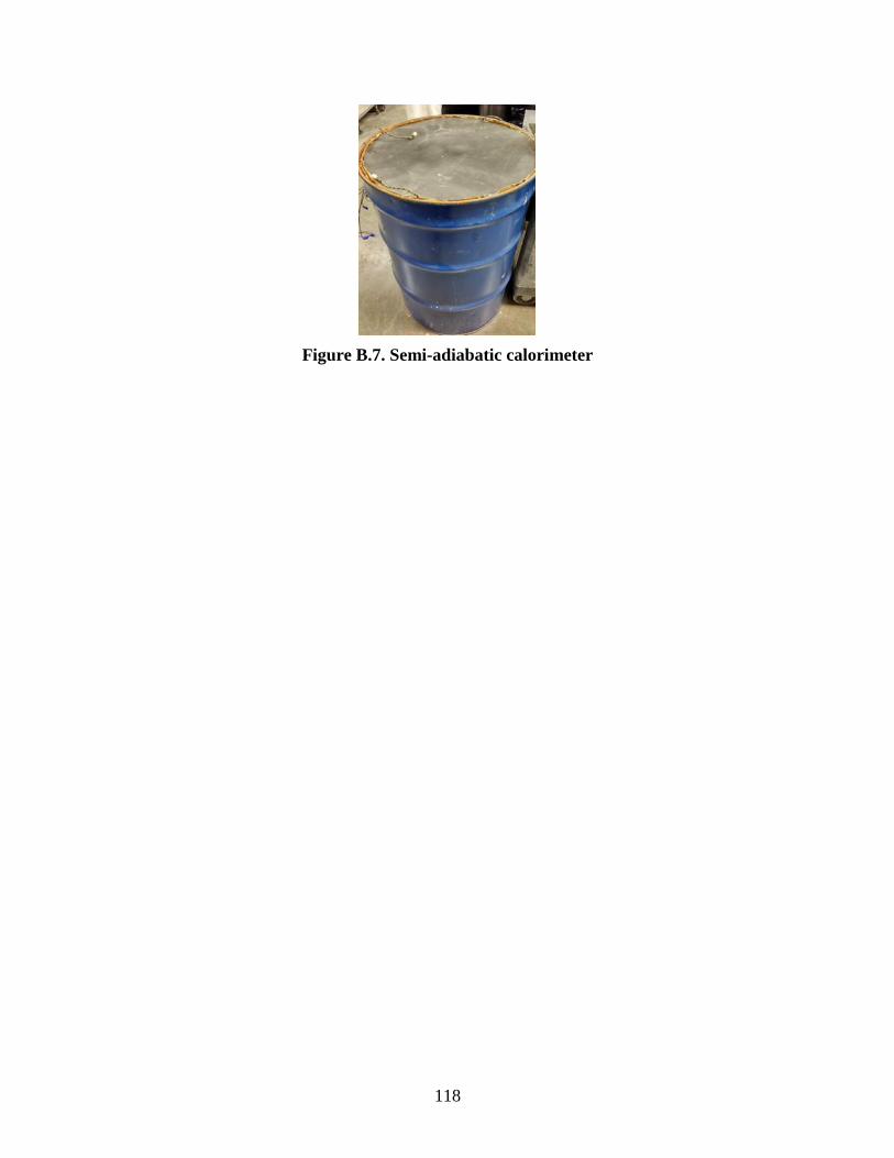
118
Figure B.7. Semi-adiabatic calorimeter
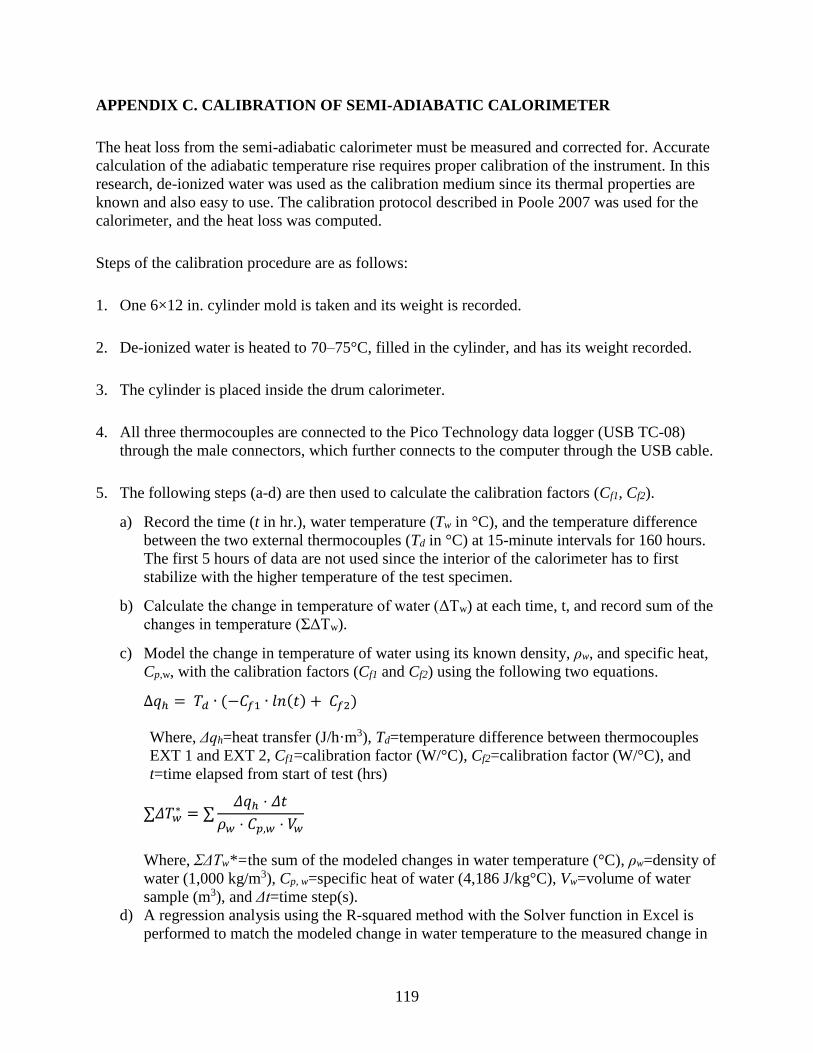
119
APPENDIX C. CALIBRATION OF SEMI-ADIABATIC CALORIMETER
The heat loss from the semi-adiabatic calorimeter must be measured and corrected for. Accurate
calculation of the adiabatic temperature rise requires proper calibration of the instrument. In this
research, de-ionized water was used as the calibration medium since its thermal properties are
known and also easy to use. The calibration protocol described in Poole 2007 was used for the
calorimeter, and the heat loss was computed.
Steps of the calibration procedure are as follows:
1. One 6×12 in. cylinder mold is taken and its weight is recorded.
2. De-ionized water is heated to 70–75°C, filled in the cylinder, and has its weight recorded.
3. The cylinder is placed inside the drum calorimeter.
4. All three thermocouples are connected to the Pico Technology data logger (USB TC-08)
through the male connectors, which further connects to the computer through the USB cable.
5. The following steps (a-d) are then used to calculate the calibration factors (Cf1, Cf2).
a) Record the time (t in hr.), water temperature (Tw in °C), and the temperature difference
between the two external thermocouples (Td in °C) at 15-minute intervals for 160 hours.
The first 5 hours of data are not used since the interior of the calorimeter has to first
stabilize with the higher temperature of the test specimen.
b) Calculate the change in temperature of water (ΔTw) at each time, t, and record sum of the
changes in temperature (ΣΔTw).
c) Model the change in temperature of water using its known density, ρw, and specific heat,
Cp,w, with the calibration factors (Cf1 and Cf2) using the following two equations.
∆𝑞ℎ = 𝑇𝑑 ∙ (−𝐶𝑓1 ∙ 𝑙𝑛(𝑡) + 𝐶𝑓2)
Where, Δqh=heat transfer (J/h·m3), Td=temperature difference between thermocouples
EXT 1 and EXT 2, Cf1=calibration factor (W/°C), Cf2=calibration factor (W/°C), and
t=time elapsed from start of test (hrs)
∑𝛥𝑇𝑤∗ = ∑
𝛥𝑞ℎ ⋅ 𝛥𝑡
𝜌𝑤 ⋅ 𝐶𝑝,𝑤 ⋅ 𝑉𝑤
Where, ΣΔTw*=the sum of the modeled changes in water temperature (°C), ρw=density of
water (1,000 kg/m3), Cp, w=specific heat of water (4,186 J/kg°C), Vw=volume of water
sample (m3), and Δt=time step(s).
d) A regression analysis using the R-squared method with the Solver function in Excel is
performed to match the modeled change in water temperature to the measured change in
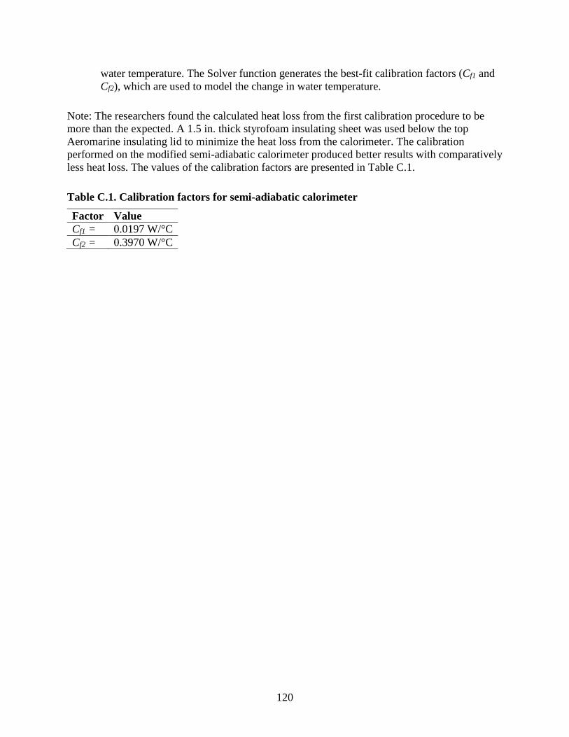
120
water temperature. The Solver function generates the best-fit calibration factors (Cf1 and
Cf2), which are used to model the change in water temperature.
Note: The researchers found the calculated heat loss from the first calibration procedure to be
more than the expected. A 1.5 in. thick styrofoam insulating sheet was used below the top
Aeromarine insulating lid to minimize the heat loss from the calorimeter. The calibration
performed on the modified semi-adiabatic calorimeter produced better results with comparatively
less heat loss. The values of the calibration factors are presented in Table C.1.
Table C.1. Calibration factors for semi-adiabatic calorimeter
Factor Value
Cf1 = 0.0197 W/°C
Cf2 = 0.3970 W/°C
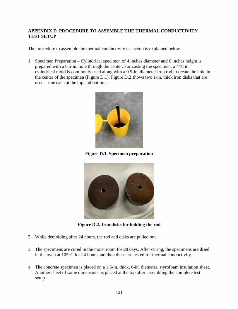
121
APPENDIX D. PROCEDURE TO ASSEMBLE THE THERMAL CONDUCTIVITY
TEST SETUP
The procedure to assemble the thermal conductivity test setup is explained below.
1. Specimen Preparation – Cylindrical specimen of 4 inches diameter and 6 inches height is
prepared with a 0.5-in. hole through the center. For casting the specimen, a 4×8 in.
cylindrical mold is commonly used along with a 0.5-in. diameter iron rod to create the hole in
the center of the specimen (Figure D.1). Figure D.2 shows two 1-in. thick iron disks that are
used—one each at the top and bottom.
Figure D.1. Specimen preparation
Figure D.2. Iron disks for holding the rod
2. While demolding after 24 hours, the rod and disks are pulled out.
3. The specimens are cured in the moist room for 28 days. After curing, the specimens are dried
in the oven at 105°C for 24 hours and then these are tested for thermal conductivity.
4. The concrete specimen is placed on a 1.5-in. thick, 6-in. diameter, styrofoam insulation sheet.
Another sheet of same dimensions is placed at the top after assembling the complete test
setup.

122
5. A total of eight temperature sensors (Type K thermocouples) are installed. The location of
sensors are as follows:
a) One sensor at one third from the top into the core of the specimen (Core top)
b) One sensor at one third from the bottom into the core of the specimen (Core bottom)
c) Five sensors at the surface of the specimen (S1, S2, S3, S4, and S5)
d) One sensor to measure the room temperature
6. The sensors at the surface are installed first. These sensors are pasted using a commonly used
black electrical tape.
7. Silicone-based high thermal conductivity paste (k = 2.3 W/m-K) manufactured by Omega
Engineering, Inc. is poured evenly into the central 0.5-in. diameter core of the specimen. The
paste is injected using a plastic tube sleeve. Effort should be made to spread the paste as
evenly and thinly as possible.
8. After the paste is poured, a cartridge heater (resistance = 57.9 Ω) of 0.375-in. diameter and 6
in. height is inserted into the core.
9. Two central thermocouples (core top and core bottom) are attached to the heater with a
separation of thin silver foil. This is done to ensure that the temperature data recorded by the
thermocouples are that of the concrete inner surface and not that of the heater.
10. The thermocouples are connected to a Pico Technology data logger (USB TC 08) for
recording temperature development during the test.
11. The heater is connected to a voltage regulator, which is connected to a power source.
12. A multimeter is also connected in series for measuring the applied voltage.
13. The resistance of the heater is measured and a predetermined voltage of 21.7 V is applied to
the heater.
14. The data recording starts at this point.
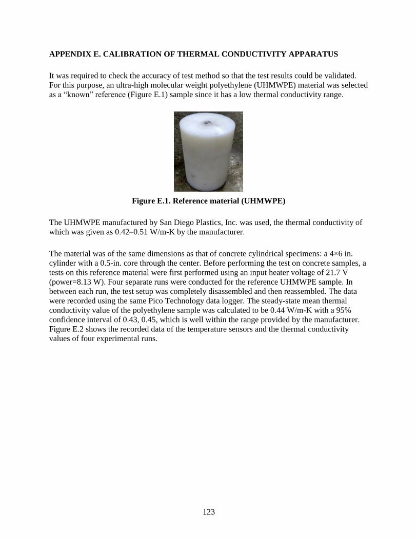
123
APPENDIX E. CALIBRATION OF THERMAL CONDUCTIVITY APPARATUS
It was required to check the accuracy of test method so that the test results could be validated.
For this purpose, an ultra-high molecular weight polyethylene (UHMWPE) material was selected
as a “known” reference (Figure E.1) sample since it has a low thermal conductivity range.
Figure E.1. Reference material (UHMWPE)
The UHMWPE manufactured by San Diego Plastics, Inc. was used, the thermal conductivity of
which was given as 0.42–0.51 W/m-K by the manufacturer.
The material was of the same dimensions as that of concrete cylindrical specimens: a 4×6 in.
cylinder with a 0.5-in. core through the center. Before performing the test on concrete samples, a
tests on this reference material were first performed using an input heater voltage of 21.7 V
(power=8.13 W). Four separate runs were conducted for the reference UHMWPE sample. In
between each run, the test setup was completely disassembled and then reassembled. The data
were recorded using the same Pico Technology data logger. The steady-state mean thermal
conductivity value of the polyethylene sample was calculated to be 0.44 W/m-K with a 95%
confidence interval of 0.43, 0.45, which is well within the range provided by the manufacturer.
Figure E.2 shows the recorded data of the temperature sensors and the thermal conductivity
values of four experimental runs.
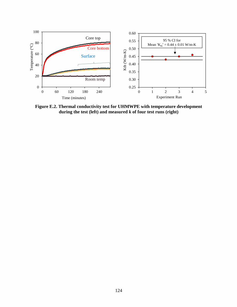
124
Figure E.2. Thermal conductivity test for UHMWPE with temperature development
during the test (left) and measured k of four test runs (right)
0
20
40
60
80
100
0 60 120 180 240
Tem
per
ature
(°C
)
Time (minutes)
Core bottom
Room temp
Core top
0.25
0.30
0.35
0.40
0.45
0.50
0.55
0.60
0 1 2 3 4 5
Kth
(W
/m-K
)
Experiment Run
95 % CI for
Mean ‘Kth’ = 0.44 ± 0.01 W/m-K
Surface
Temp


THE INSTITUTE FOR TRANSPORTATION IS THE FOCAL POINT FOR TRANSPORTATION AT IOWA STATE UNIVERSITY.
InTrans centers and programs perform transportation research and provide technology transfer services for government agencies and private companies;
InTrans contributes to Iowa State University and the College of Engineering’s educational programs for transportation students and provides K–12 outreach; and
InTrans conducts local, regional, and national transportation services and continuing education programs.
Visit InTrans.iastate.edu for color pdfs of this and other research reports.
Top Related