


Languages
Pages
Legal


Estimating the Size of the Shadow
Economy: Methods and Problems;
and the Latest Results for the
Baltic Countries
Prof. Dr. DDr.h.c. Friedrich Schneider
Department of Economics
Johannes Kepler University of Linz
A-4040 Linz-Auhof
ShadEcEstimation_BalticCountries.ppt
E-mail: [email protected]
Phone: 0043-732-2468-8210
Fax: 0043-732-2468-8209
http://www.econ.jku.at
Revised Version
July 17, 2014
July 2014 Prof. Dr. Friedrich Schneider, University of Linz / AUSTRIA 1 of 44

All over the world, empirical research about the size
and development of the shadow economy has strongly
increased. However, most empirical results are heavily
disputed by many economists around the world.
Hence, the first goal of this lecture is to review the
various methods estimating the size of the shadow
economy and to discuss their strengths and weaknesses;
the second one is to present some results for the Baltic
countries.
1. Introduction
July 2014 Prof. Dr. Friedrich Schneider, University of Linz / AUSTRIA 2 of 44
1) Introduction
2) Defining the Shadow Economy
3) Methods to Estimate the Size of the Shadow Economy
4) Results of the Size of the German Shadow Economy
Using the Various Estimation Methods
5) Size of the Shadow Economies of the Baltic States
6) Concluding Remarks: Problems and Open Questions
7) Appendix: A Comparison between the MIMIC and
Survey Method
Content
July 2014 Prof. Dr. Friedrich Schneider, University of Linz / AUSTRIA 3 of 44
2. Defining the Shadow Economy
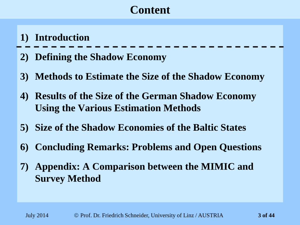
Type of activity Monetary transactions Non-monetary transactions Illegal
Activities
Trade with stolen goods; drug
dealing and manufacturing;
prostitution; gambling; fraud;
etc.
Barter of drugs, stolen goods,
smuggling etc. Produce drugs
for own use. Theft for own use.
Tax Evasion
Tax Avoidance
Tax Evasion
Tax Avoidance
Legal
Activities
Unreported
income from
self-
employment;
wages, salaries
and assets
from
unreported
work
Employee
discounts,
fringe benefits
Barter of legal
services and
goods
All do-it-
yourself work;
neighbor help;
and voluntary
work
Table 2.1: A taxonomy of types of underground economic activities
Structure of the table is taken from Lippert and Walker (1997, p. 5) with additional remarks
July 2014 Prof. Dr. Friedrich Schneider, University of Linz / AUSTRIA 4 of 44

The shadow economy includes all market-based legal
production of goods and services that are deliberately
concealed from public authorities for the following
reasons:
(1) to avoid payment of income and/or indirect taxes,
(2) to avoid payment of social security contributions,
(3) to avoid certain legal labor market standards, such
as minimum wages, maximum working hours,
safety standards, etc., and
(4) to avoid complying with certain administrative
procedures.
2. Defining the Shadow Economy
July 2014 Prof. Dr. Friedrich Schneider, University of Linz / AUSTRIA 5 of 44
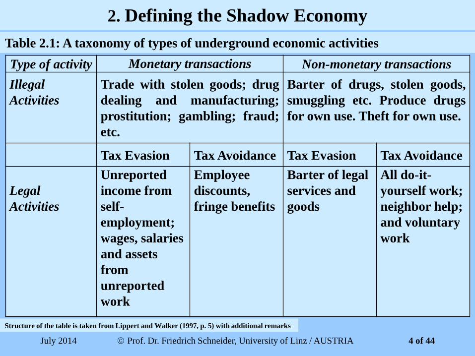
(1) Underground (classical crime) activities are all
illegal actions that fit the characteristics of classical
crime activities like burglary, robbery, drug
dealing, etc.
(2) Informal household economy consists of household
enterprises that are not registered officially under
various specific forms of national legislation.
To a large extent these two sectors are not included in
the shadow economy activities.
2. Defining the Underground and Informal Household Economy
July 2014 Prof. Dr. Friedrich Schneider, University of Linz / AUSTRIA 6 of 44
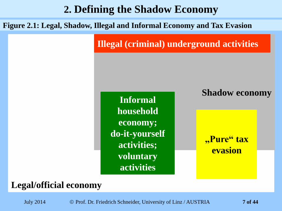
Figure 2.1: Legal, Shadow, Illegal and Informal Economy and Tax Evasion
Legal/official economy
Shadow economy
Illegal (criminal) underground activities
Informal
household
economy;
do-it-yourself
activities;
voluntary
activities
„Pure“ tax
evasion
2. Defining the Shadow Economy
July 2014 Prof. Dr. Friedrich Schneider, University of Linz / AUSTRIA 7 of 44

There are three major approaches to measure the
shadow economy:
(1) direct ones,
(2) indirect ones, and the
(3) model or latent variable (MIMIC = multiple
indicators multiple causes) one.
3. Methods to Estimate the Size of the Shadow Economy
July 2014 Prof. Dr. Friedrich Schneider, University of Linz / AUSTRIA 8 of 44
(1) These are microeconomic approaches that employ
either well designed surveys or samples based on
voluntary replies or tax auditing and other
compliance methods.
(2) Estimates of the shadow economy can also be based
on the discrepancy between income declared for tax
purposes and the actual detected one by audits.
Advantage of (1) and (2): Detailed knowledge about the
shadow economy on an individual basis.
3. Methods to Estimate the Size of the Shadow Economy 3.1 Direct Approaches
July 2014 Prof. Dr. Friedrich Schneider, University of Linz / AUSTRIA 9 of 44
Disadvantages of (1) and (2):
(i) Survey methods are likely to underestimate the
shadow economy because in surveys people are
likely to under-declare what they are hiding from
authorities.
In order to minimize this behavior structured
interviews are undertaken (usually face to face).
(ii) A further disadvantage of these two direct methods
(surveys and tax auditing) is the point estimate
character.
3. Methods to Estimate the Size of the Shadow Economy 3.1 Direct Approaches
July 2014 Prof. Dr. Friedrich Schneider, University of Linz / AUSTRIA 10 of 44
These approaches, which are also called “indicator”
approaches, are mostly macroeconomic ones and use various
(mostly economic) indicators that contain information about
the development of the shadow economy (over time).
Five indicator approaches:
3.2.1 The Discrepancy between National Expenditure and Income Statistics;
3.2.2 The Discrepancy between the Official and Actual Labor Force;
3.2.3 The Transactions Approach;
3.2.4 The Currency Demand Approach; and
3.2.5 The Physical Input (Electricity Consumption) Method.
3. Methods to Estimate the Size of the Shadow Economy 3.2 Indirect Approaches
July 2014 Prof. Dr. Friedrich Schneider, University of Linz / AUSTRIA 11 of 44
(1) This approach is based on discrepancies between
income and expenditure statistics.
(2) In national accounting the income measure of GNP
should be equal to the expenditure measure of GNP.
(3) If an independent estimate of the expenditure site of
the national accounts is available, the gap between
the expenditure measure and the income measure is
an indicator of the size of the shadow economy.
3. Methods to Estimate the Size of the Shadow Economy 3.2.1 The Discrepancy between National Expenditure and Income Statistics
July 2014 Prof. Dr. Friedrich Schneider, University of Linz / AUSTRIA 12 of 44
(4) If all the components of the expenditure site where
measured without error, then this approach would
indeed yield a good estimate of the scale of the
shadow economy.
(5) However, unfortunately, this is not the case and the
discrepancy, therefore, reflects all omissions and
errors everywhere in the national accounts statistics
as well as the shadow economy activity.
3. Methods to Estimate the Size of the Shadow Economy 3.2.1 The Discrepancy between National Expenditure and Income Statistics
July 2014 Prof. Dr. Friedrich Schneider, University of Linz / AUSTRIA 13 of 44

(1) If total labor force participation is assumed to be
constant, a decreasing official rate of participation
can be an indicator of an increase in the activities in
the shadow economy, ceteris paribus.
(2) One weakness of this method is that differences in
the rate of participation also have other causes.
(3) Moreover, people can work in the shadow economy
and have a job in the „official’ economy.
3. Methods to Estimate the Size of the Shadow Economy 3.2.2 The Discrepancy between the Official and Actual Labor Force
July 2014 Prof. Dr. Friedrich Schneider, University of Linz / AUSTRIA 14 of 44

(1) This approach has been developed by Edgar Feige. He
assumes, that over time there is a constant relation
between the volume of total transactions and total GNP.
(2) Feige’s approach starts from Fisher’s quantity equation:
M*V = p*T,
with
(3) Assumptions are necessary about the velocity of money
and about the relationships between the value of total
transactions (p*T) and total (=official + unofficial)
nominal GNP.
3. Methods to Estimate the Size of the Shadow Economy 3.2.3 The Transactions Approach
M = money
V = velocity
p = prices
T = total transactions
July 2014 Prof. Dr. Friedrich Schneider, University of Linz / AUSTRIA 15 of 44
(4) Relating total nominal GNP to total transactions, the
GNP of the shadow economy can be calculated by
subtracting the official GNP from total nominal GNP.
(5) To derive figures for the shadow economy, Feige has to
assume a base year, in which there is no shadow
economy, and therefore the ratio of p*T to total nominal
(official = total) GNP was „normal“ and would have
been constant over time, if there had been no shadow
economy.
3. Methods to Estimate the Size of the Shadow Economy 3.2.3 The Transactions Approach
July 2014 Prof. Dr. Friedrich Schneider, University of Linz / AUSTRIA 16 of 44

(6) Weaknesses:
(i) the assumption of a base year with no shadow
economy;
(ii) the assumption of a „normal“ ratio of transactions
constant over time;
(iii) to obtain reliable estimates, precise figures of the
total volume of transactions should be available;
(iv) This is difficult to achieve for cash transactions,
because they depend, among other factors, on the
durability of bank notes, in terms of the quality of
the paper on which they are printed; and
3. Methods to Estimate the Size of the Shadow Economy 3.2.3 The Transactions Approach
July 2014 Prof. Dr. Friedrich Schneider, University of Linz / AUSTRIA 17 of 44
(6) Weaknesses (cont.):
(v) in an “ideal” situation all variations in the ratio
between the total value of transaction and the
officially measured GNP are due to the shadow
economy.
This means that a considerable amount of data is
required in order to eliminate financial transactions
from “pure” cross payments, which are totally legal
and have nothing to do with the shadow economy.
In general, although this approach is theoretically very
attractive, the empirical requirements necessary to obtain
reliable estimates are so difficult to fulfill that in most cases
its application leads to quite high results.
3. Methods to Estimate the Size of the Shadow Economy 3.2.3 The Transactions Approach
July 2014 Prof. Dr. Friedrich Schneider, University of Linz / AUSTRIA 18 of 44
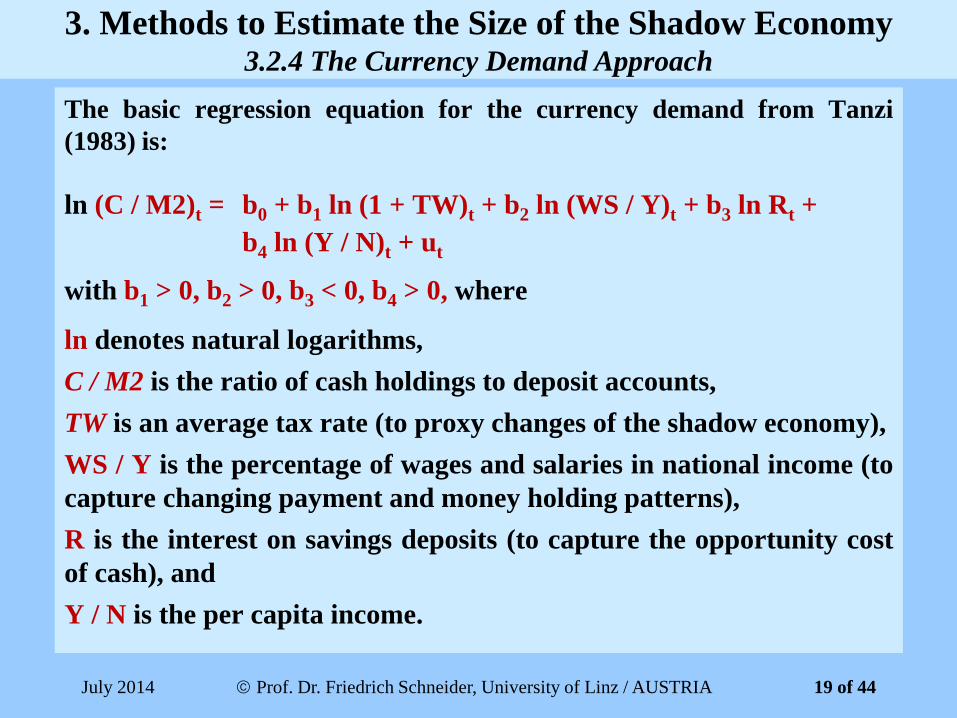
The basic regression equation for the currency demand from Tanzi
(1983) is:
ln (C / M2)t = b0 + b1 ln (1 + TW)t + b2 ln (WS / Y)t + b3 ln Rt +
b4 ln (Y / N)t + ut
with b1 > 0, b2 > 0, b3 < 0, b4 > 0, where
ln denotes natural logarithms,
C / M2 is the ratio of cash holdings to deposit accounts,
TW is an average tax rate (to proxy changes of the shadow economy),
WS / Y is the percentage of wages and salaries in national income (to
capture changing payment and money holding patterns),
R is the interest on savings deposits (to capture the opportunity cost
of cash), and
Y / N is the per capita income.
3. Methods to Estimate the Size of the Shadow Economy 3.2.4 The Currency Demand Approach
July 2014 Prof. Dr. Friedrich Schneider, University of Linz / AUSTRIA 19 of 44
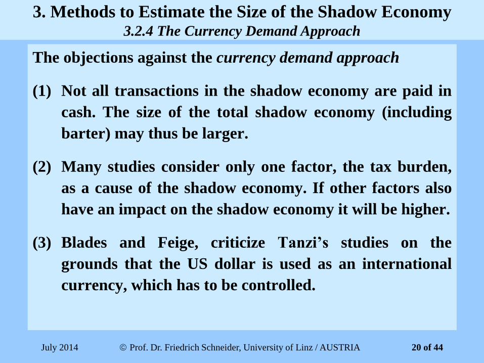
The objections against the currency demand approach
(1) Not all transactions in the shadow economy are paid in
cash. The size of the total shadow economy (including
barter) may thus be larger.
(2) Many studies consider only one factor, the tax burden,
as a cause of the shadow economy. If other factors also
have an impact on the shadow economy it will be higher.
(3) Blades and Feige, criticize Tanzi’s studies on the
grounds that the US dollar is used as an international
currency, which has to be controlled.
3. Methods to Estimate the Size of the Shadow Economy 3.2.4 The Currency Demand Approach
July 2014 Prof. Dr. Friedrich Schneider, University of Linz / AUSTRIA 20 of 44
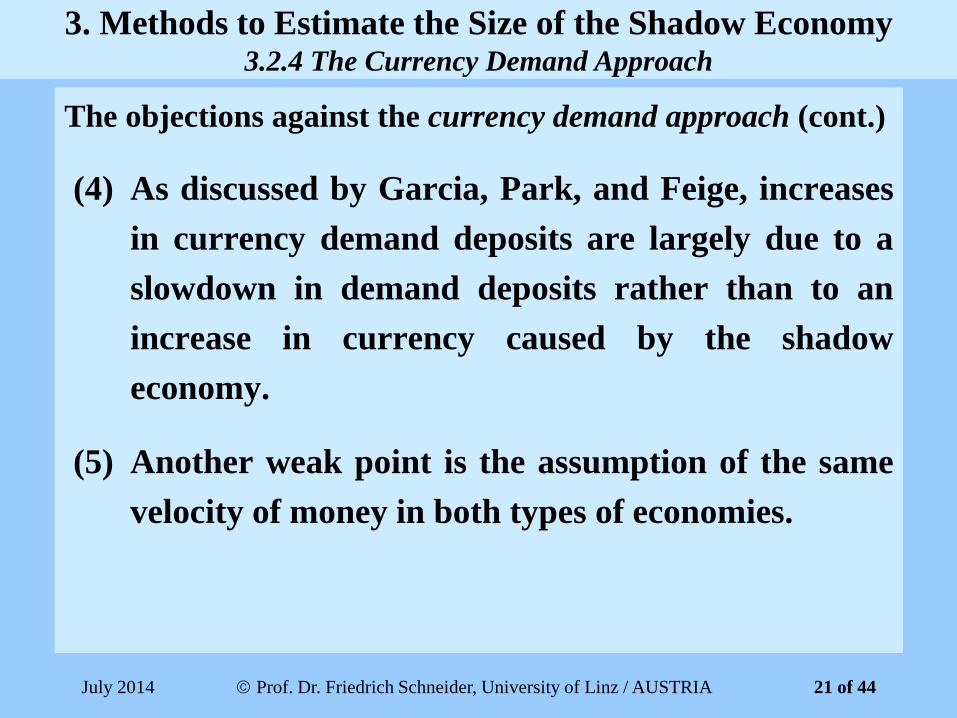
The objections against the currency demand approach (cont.)
(4) As discussed by Garcia, Park, and Feige, increases
in currency demand deposits are largely due to a
slowdown in demand deposits rather than to an
increase in currency caused by the shadow
economy.
(5) Another weak point is the assumption of the same
velocity of money in both types of economies.
3. Methods to Estimate the Size of the Shadow Economy 3.2.4 The Currency Demand Approach
July 2014 Prof. Dr. Friedrich Schneider, University of Linz / AUSTRIA 21 of 44

The objections against the currency demand approach (cont.)
(6) Ahumada, Canavese and Canavese (2004) show,
that the assumption of equal income velocity of
money in both economies is only correct, if the
income elasticity is 1; if this is not the case, the
calculation has to be corrected.
(7) Finally, the assumption of no shadow economy in a
base year is open to criticism.
3. Methods to Estimate the Size of the Shadow Economy 3.2.4 The Currency Demand Approach
July 2014 Prof. Dr. Friedrich Schneider, University of Linz / AUSTRIA 22 of 44
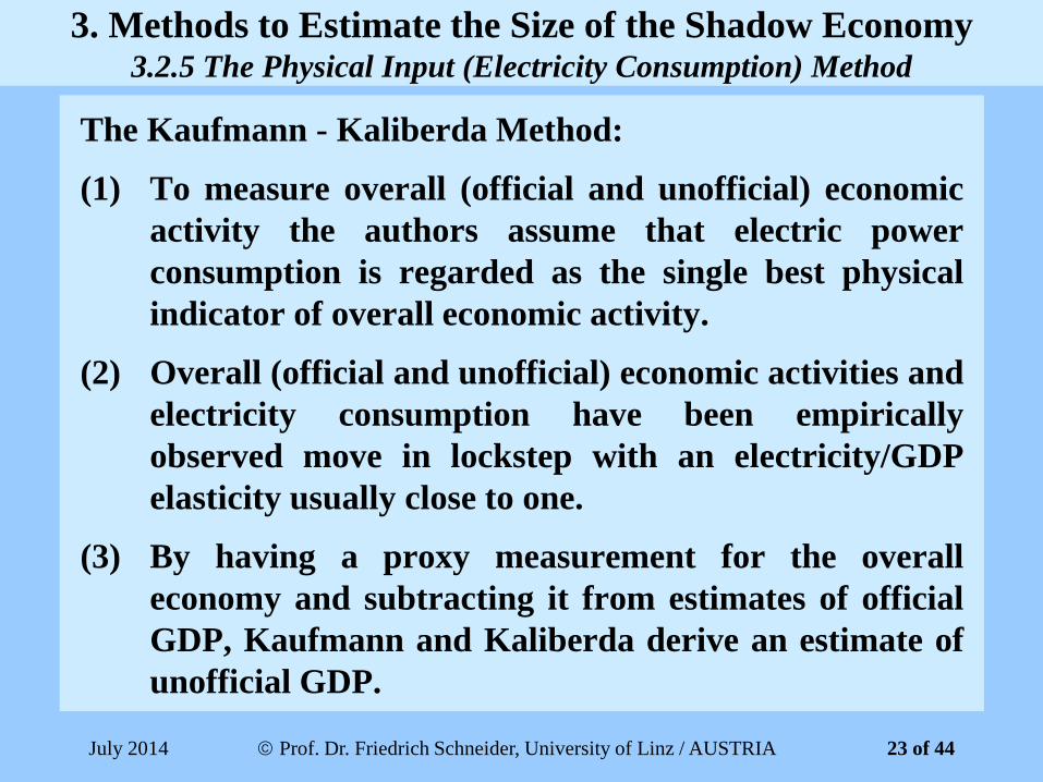
The Kaufmann - Kaliberda Method:
(1) To measure overall (official and unofficial) economic
activity the authors assume that electric power
consumption is regarded as the single best physical
indicator of overall economic activity.
(2) Overall (official and unofficial) economic activities and
electricity consumption have been empirically
observed move in lockstep with an electricity/GDP
elasticity usually close to one.
(3) By having a proxy measurement for the overall
economy and subtracting it from estimates of official
GDP, Kaufmann and Kaliberda derive an estimate of
unofficial GDP.
3. Methods to Estimate the Size of the Shadow Economy 3.2.5 The Physical Input (Electricity Consumption) Method
July 2014 Prof. Dr. Friedrich Schneider, University of Linz / AUSTRIA 23 of 44
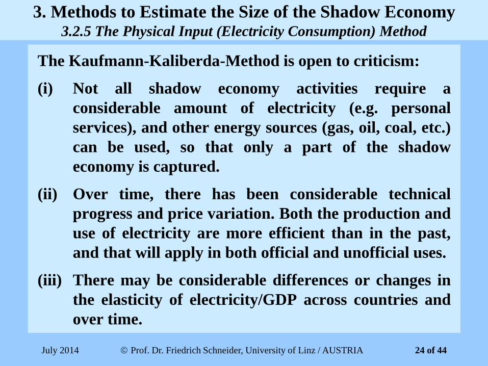
The Kaufmann-Kaliberda-Method is open to criticism:
(i) Not all shadow economy activities require a
considerable amount of electricity (e.g. personal
services), and other energy sources (gas, oil, coal, etc.)
can be used, so that only a part of the shadow
economy is captured.
(ii) Over time, there has been considerable technical
progress and price variation. Both the production and
use of electricity are more efficient than in the past,
and that will apply in both official and unofficial uses.
(iii) There may be considerable differences or changes in
the elasticity of electricity/GDP across countries and
over time.
3. Methods to Estimate the Size of the Shadow Economy 3.2.5 The Physical Input (Electricity Consumption) Method
July 2014 Prof. Dr. Friedrich Schneider, University of Linz / AUSTRIA 24 of 44
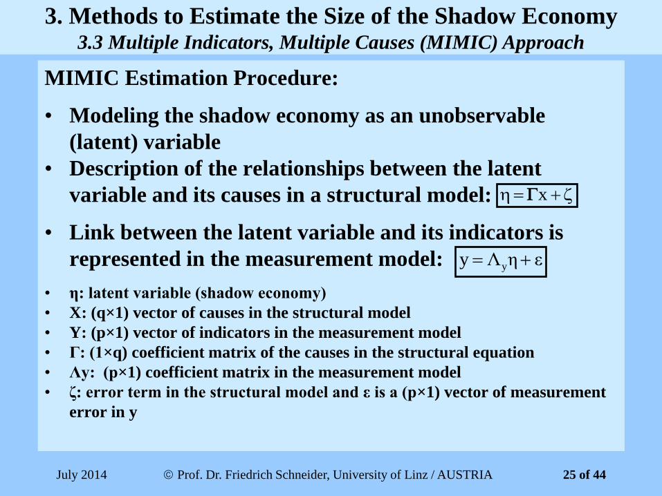
MIMIC Estimation Procedure:
• Modeling the shadow economy as an unobservable
(latent) variable
• Description of the relationships between the latent
variable and its causes in a structural model:
• Link between the latent variable and its indicators is
represented in the measurement model:
• η: latent variable (shadow economy)
• X: (q×1) vector of causes in the structural model
• Y: (p×1) vector of indicators in the measurement model
• Γ: (1×q) coefficient matrix of the causes in the structural equation
• Λy: (p×1) coefficient matrix in the measurement model
• ζ: error term in the structural model and ε is a (p×1) vector of measurement
error in y
x
εηΛy y
3. Methods to Estimate the Size of the Shadow Economy 3.3 Multiple Indicators, Multiple Causes (MIMIC) Approach
July 2014 Prof. Dr. Friedrich Schneider, University of Linz / AUSTRIA 25 of 44

MIMIC Estimation Procedure (cont.):
► Specification of structural equation:
[shadow economy ] = [ γ1, γ2, γ3, γ4, γ5, γ6, γ7, γ8] x
► Specification of measurement equation:
Employment Quota λ1 ε1
Change of local currency = λ2 x + ε2
Average working time λ3 ε3
[Share of direct taxation]
[Share of indirect taxation]
[Share of social security burden]
[Burden of state regulation] + [ζ]
[Quality of state institutions]
[Tax morale]
[Unemployment quota]
[GDP per capita]
Shadow
Economy
3. Methods to Estimate the Size of the Shadow Economy 3.3 Multiple Indicators, Multiple Causes (MIMIC) Approach
July 2014 Prof. Dr. Friedrich Schneider, University of Linz / AUSTRIA 26 of 44
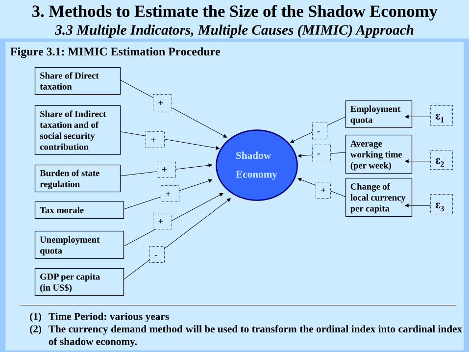
Figure 3.1: MIMIC Estimation Procedure
Share of Direct
taxation
Burden of state
regulation
Employment
quota
Change of
local currency
per capita
Average
working time
(per week)
Share of Indirect
taxation and of
social security
contribution
Tax morale
Unemployment
quota
GDP per capita
(in US$)
Shadow
Economy
+
ε1
ε2
ε3
(1) Time Period: various years
(2) The currency demand method will be used to transform the ordinal index into cardinal index
of shadow economy.
+
+
+
+
-
-
-
+
3. Methods to Estimate the Size of the Shadow Economy 3.3 Multiple Indicators, Multiple Causes (MIMIC) Approach
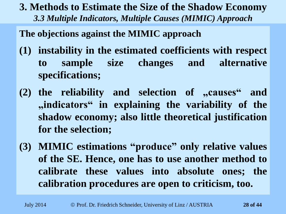
The objections against the MIMIC approach
(1) instability in the estimated coefficients with respect
to sample size changes and alternative
specifications;
(2) the reliability and selection of „causes“ and
„indicators“ in explaining the variability of the
shadow economy; also little theoretical justification
for the selection;
(3) MIMIC estimations “produce” only relative values
of the SE. Hence, one has to use another method to
calibrate these values into absolute ones; the
calibration procedures are open to criticism, too.
3. Methods to Estimate the Size of the Shadow Economy 3.3 Multiple Indicators, Multiple Causes (MIMIC) Approach
July 2014 Prof. Dr. Friedrich Schneider, University of Linz / AUSTRIA 28 of 44

The objections against the MIMIC approach (cont.)
(4) Another critique concerns the meaning of the latent
variable. As the latent variable and its unit of
measurement are not observed, the MIMIC
procedure just provides a set of estimated
coefficients from which one can calculate an index
that shows the dynamics of the unobservable
variable;
(5) The application of the calibration or benchmarking
procedure requires experimentation, and a
comparison of the calibrated values in a wide
academic debate.
3. Methods to Estimate the Size of the Shadow Economy 3.3 Multiple Indicators, Multiple Causes (MIMIC) Approach
July 2014 Prof. Dr. Friedrich Schneider, University of Linz / AUSTRIA 29 of 44

4. Results of the Size of the German Shadow Economy Using the
Various Estimation Methods
Table 4.1: The Size of the Shadow Economy in Germany According to Different
Methods (in percentage of official GDP)
Method/Source Shadow economy (in percentage of official GDP) in:
1970 1975 1980 1985 1990 1995 2000 2005
Survey Approach
(IfD Allensbach, 1975
(1st row); Feld and
Larsen, 2005 (2nd and
3rd row))
- 3.6 1) - - - - - -
- - - - - - 4.1 2) 3.1 2)
- - - - - - 1.3 3) 1.0 3)
Discrepancy between
expenditure and
income (Lippert and
Walker, 1997)
11.0 10.2 13.4 - - - - -
Discrepancy between
official and actual
employment
(Langfeldt, 1983)
23.0 38.5 34.0 - - - - -
1) 1974.
2) 2001 and 2004; calculated using wages in the official economy.
3) 2001 and 2004; calculated using actual “black” hourly wages paid. 30 of 44

4. Results of the Size of the German Shadow Economy Using the
Various Estimation Methods
Table 4.1: The Size of the Shadow Economy in Germany According to Different
Methods (in percentage of official GDP) (cont.)
Method/Source Shadow economy (in percentage of official GDP) in:
1970 1975 1980 1985 1990 1995 2000 2005
Physical input method
(Feld and Larsen, 2005) - - - 14.5 14.6 - - -
Transactions approach 17.2 22.3 29.3 31.4 - - - -
Currency demand
approach (Kirchgässner,
1983 (1st row); Langfeldt,
1983, 1984 (2nd row);
Schneider and Enste, 2000
(3rd row))
3.1 6.0 10.3 - - - - -
12.1 11.8 12.6 - - - - -
4.5 7.8 9.2 11.3 11.8 12.5 14.7 -
Latent (MIMIC)
approach (Frey and
Weck, 1983 (1st row);
Pickardt and Sarda, 2006
(2nd row); Schneider, 2005,
2007 (3rd row))
5.8 6.1 8.2 - - - - -
- - 9.4 10.1 11.4 15.1 16.3 -
4.2 5.8 10.8 11.2 12.2 13.9 16.0 15.4
July 2014
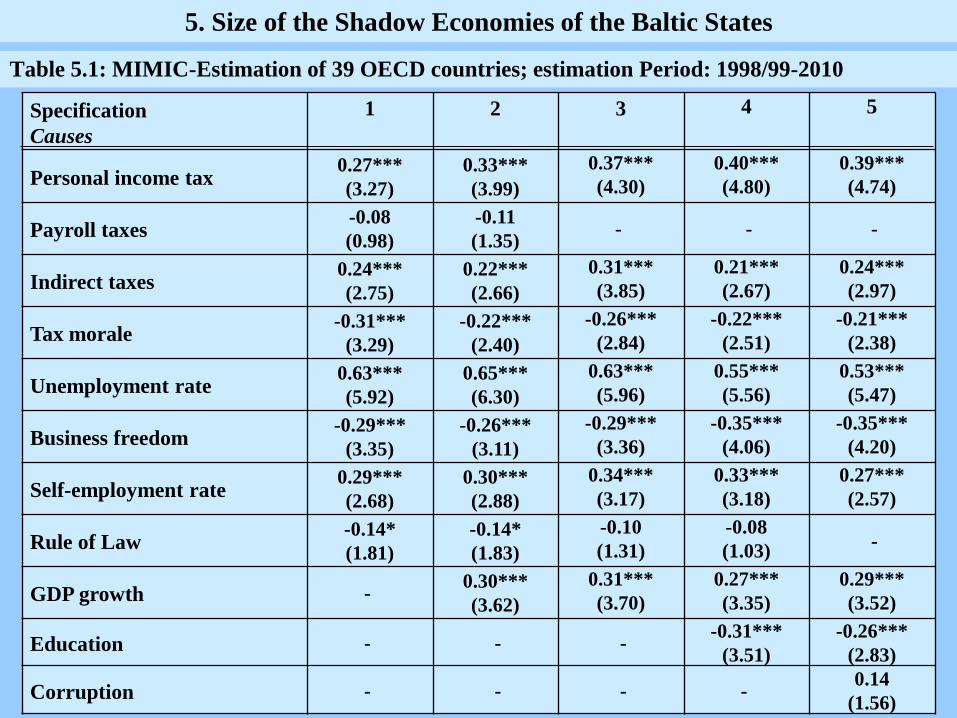
Table 5.1: MIMIC-Estimation of 39 OECD countries; estimation Period: 1998/99-2010
Prof. Dr. Friedrich Schneider, University of Linz / AUSTRIA
Specification
Causes
1
2
3
4
5
Personal income tax 0.27***
(3.27)
0.33***
(3.99)
0.37***
(4.30)
0.40***
(4.80)
0.39***
(4.74)
Payroll taxes -0.08
(0.98)
-0.11
(1.35) - - -
Indirect taxes 0.24***
(2.75)
0.22***
(2.66)
0.31***
(3.85)
0.21***
(2.67)
0.24***
(2.97)
Tax morale -0.31***
(3.29)
-0.22***
(2.40)
-0.26***
(2.84)
-0.22***
(2.51)
-0.21***
(2.38)
Unemployment rate 0.63***
(5.92)
0.65***
(6.30)
0.63***
(5.96)
0.55***
(5.56)
0.53***
(5.47)
Business freedom -0.29***
(3.35)
-0.26***
(3.11)
-0.29***
(3.36)
-0.35***
(4.06)
-0.35***
(4.20)
Self-employment rate 0.29***
(2.68)
0.30***
(2.88)
0.34***
(3.17)
0.33***
(3.18)
0.27***
(2.57)
Rule of Law -0.14*
(1.81)
-0.14*
(1.83)
-0.10
(1.31)
-0.08
(1.03) -
GDP growth - 0.30***
(3.62)
0.31***
(3.70)
0.27***
(3.35)
0.29***
(3.52)
Education - - - -0.31***
(3.51)
-0.26***
(2.83)
Corruption - - - - 0.14
(1.56)
5. Size of the Shadow Economies of the Baltic States

Table 5.1: MIMIC-Estimation of 39 OECD countries; estimation Period: 1998/99-2010 (cont.)
Prof. Dr. Friedrich Schneider, University of Linz / AUSTRIA
Indicators 1 2 3 4 5
GDP pc -0.52 -0.52 -0.48 -0.51 -0.50
Currency in circulation
per capita
0.09
(1.39)
0.07
(1.07)
0.10*
(1.75)
0.10*
(1.69)
0.08
(1.26)
Labour force
participation rate -0.56***
(6.42)
-0.55***
(6.58)
-0.52***
(6.36)
-0.50***
(6.48)
-0.51***
(6.46)
Observations 151 151 151 151 151
Degrees of Freedom 44 54 42 52 52
Chi-squared 88.88 89.68 24.10 32.51 34.57
RMSEA 0.08 0.06 0.00 0.00 0.00
Note: The sample includes 39 OECD countries and the estimation period is 1998 to 2010. Absolute z-statistics
are reported in parentheses. * , **, *** indicate significance at the 10%, 5%, and 1% level, respectively.
July 2014
5. Size of the Shadow Economies of the Baltic States
33 of 44
Prof. Dr. Friedrich Schneider, University of Linz / AUSTRIA
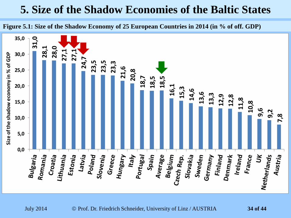
Figure 5.1: Size of the Shadow Economy of 25 European Countries in 2014 (in % of off. GDP)
July 2014
5. Size of the Shadow Economies of the Baltic States
31
,0
28
,1
28
,0
27
,1
27
,1
24
,7
23
,5
23
,5
23
,3
21
,6
20
,8
18
,7
18
,5
18
,5
16
,1
15
,3
14
,6
13
,6
13
,3
12
,9
12
,8
11
,8
10
,8
9,6
9,2
7,8
0,0
5,0
10,0
15,0
20,0
25,0
30,0
35,0
Size
of t
he
sh
ado
w e
con
om
y in
% o
f G
DP
34 of 44
Country 2009 2010 2011 2012 2013 2013 -
2012
Estimation
Method
Estonia1) 20.2%
(18.7, 21.7)
19.4%
(18.0, 20.8)
18.9%
(16.8, 20.9)
19.2%
(16.6, 21.9)
15.7%
(13.5, 17.9)
-3.5%
(-5.9, -1.1)
Index
Approach
Estonia2) 29.6%
(28.0, 31.2)
29.3%
(27.7, 30.9)
28.6%
(27.0, 30.2)
28.2%
(26.6, 29.8)
27.6%
(26.0, 29.2) -0,6% MIMIC
Latvia1) 36.6%
(34.3, 38.9)
38.1%
(35.9, 40.3)
30.2%
(27.6, 32.7)
21.1%
(18.5, 23.6)
23.8%
(20.7, 26.9)
+2.7%
(-0.1, +5.6)
Index
Approach
Latvia2) 27.1%
(24.7, 29.5)
27.3%
(24.9, 29.7)
26.5%
(24.1, 28.9)
26.1%
(23.7, 28.5)
25.5%
(23.1, 27.9) -0,6% MIMIC
Lithuania1) 17.7%
(15.8, 19.7)
18.8%
(16.9, 20.6)
17.1%
(15.2, 19.0)
18.2%
(16.4, 20.1)
15.3%
(13.6, 17.1)
-2.9%
(-4.7, -1.1)
Index
Approach
Lithuania2) 29.6%
(27.7, 31.5)
29.7%
(27.8-31.6)
29.0%
(27.1, 30.9)
28.5%
(26.6, 30.4)
28.0%
(26.1, 29.9) -0.5% MIMIC
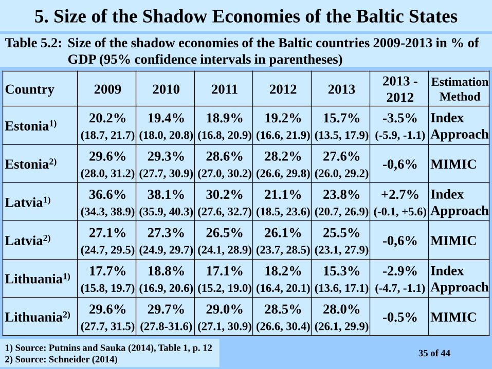
Table 5.2: Size of the shadow economies of the Baltic countries 2009-2013 in % of
GDP (95% confidence intervals in parentheses)
1) Source: Putnins and Sauka (2014), Table 1, p. 12
2) Source: Schneider (2014)
5. Size of the Shadow Economies of the Baltic States
35 of 44
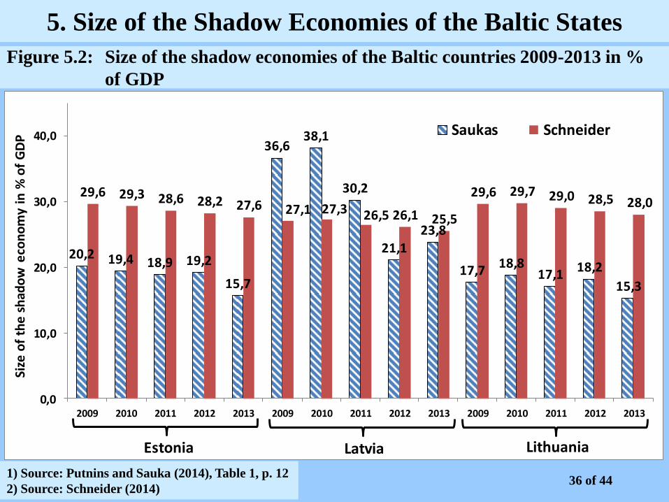
Figure 5.2: Size of the shadow economies of the Baltic countries 2009-2013 in %
of GDP
1) Source: Putnins and Sauka (2014), Table 1, p. 12
2) Source: Schneider (2014)
5. Size of the Shadow Economies of the Baltic States
20,2 19,4 18,9 19,2
15,7
36,638,1
30,2
21,123,8
17,718,8
17,118,2
15,3
29,6 29,3 28,6 28,2 27,6 27,1 27,3 26,5 26,1 25,5
29,6 29,7 29,0 28,5 28,0
0,0
10,0
20,0
30,0
40,0
2009 2010 2011 2012 2013 2009 2010 2011 2012 2013 2009 2010 2011 2012 2013
Size
of
the
sh
ado
w e
con
om
y in
% o
f G
DP
Saukas Schneider
Estonia Latvia Lithuania
36 of 44

6.1 Surveys:
(1) Quite often only households or only partly firms are
considered.
(2) Non-responses and/or incorrect responses
(3) Results of the financial volume of „black“ hours
worked and not of value added.
6. Concluding Remarks: Problems
July 2014 Prof. Dr. Friedrich Schneider, University of Linz / AUSTRIA 37 of 44

6.2 Discrepancy Method:
(1) Combination of meso estimates/assumptions
(2) Calculation method often not clear
(3) Documentation and procedures often not public
6. Concluding Remarks: Problems
July 2014 Prof. Dr. Friedrich Schneider, University of Linz / AUSTRIA 38 of 44
6.3 Monetary and/or Electricity Methods:
(1) Some estimates are very high and only macro-estimates.
(2) Are the assumptions about shadow economy activities
plausible?
(3) Breakdown by sector or industry not possible!
(4) Great differences to convert millions of KWh into a
value added figure when using the electricity method
(Lackó approach).
6. Concluding Remarks: Problems
July 2014 Prof. Dr. Friedrich Schneider, University of Linz / AUSTRIA 39 of 44

6.4 MIMIC (Latent) Method:
(1) Only relative coefficients, no absolute values.
(2) Estimations quite often highly sensitive with
respect to changes in the data and specifications.
(3) Difficulty to differentiate between the selection of
causes and indicators; little theoretical “guidance”.
(4) The use of the calibration procedure and starting
values has great influence on the size and
development of the shadow economy.
6. Concluding Remarks: Problems
July 2014 Prof. Dr. Friedrich Schneider, University of Linz / AUSTRIA 40 of 44
(1) No ideal or dominating method – all have
serious problems and weaknesses.
(2) If possible use several methods.
(3) Much more research is needed with respect to
the estimation methodology and empirical
results for different countries and periods.
(4) Experimental methods should be used to
provide a micro-foundation.
6. Concluding Remarks: Final Statements
July 2014 Prof. Dr. Friedrich Schneider, University of Linz / AUSTRIA 41 of 44

(1) A common and internationally accepted definition
of the shadow economy is still missing. Such a
definition or convention is needed in order to make
comparisons between countries easier.
(2) A satisfactory validation of the empirical results
should be developed so that it is easier to judge the
empirical results with respect to their plausibility.
6. Concluding Remarks: Open Research Questions
July 2014 Prof. Dr. Friedrich Schneider, University of Linz / AUSTRIA 42 of 44
(3) The link between theory and empirical estimation
of the shadow economy is still unsatisfactory.
In the best case theory provides us with derived
signs of the causal and indicator variables.
However, which are the “core” causal and which
are the “core” indicator variables is theoretically
„open“.
6. Concluding Remarks: Open Research Questions
July 2014 Prof. Dr. Friedrich Schneider, University of Linz / AUSTRIA 43 of 44

Thank you very much for your
attention!
July 2014 Prof. Dr. Friedrich Schneider, University of Linz / AUSTRIA 44 of 44

Table A.1: A comparison of the Size of the German Shadow Economy using the
survey and the MIMIC-method, year 2006
Various kinds of shadow economy
activities/values
Shadow
Economy in
% of official
GDP
Shadow
Economy
in bill.
Euro
% share of the
overall shadow
economy
Shadow economy activities from labour
(hours worked, survey results)
+ Material (used)
+ Illegal activities (goods and services)
+ already in the official GDP included
illegal activities
5.0 – 6.0
3.0 – 4.0
4.0 – 5.0
1.0 – 2.0
117 – 140
70 – 90
90 – 117
23 – 45
33 – 40
20 – 25
25 – 33
7 - 13
Sum (1) to (4) 13.0 – 17.0 300 – 392 85 – 111
Overall (total) shadow economy
(estimated by the MIMIC and
calibrated by the currency demand
procedure)
15.0 340 100
Source: Enste/Schneider (2006) and own calculations.
Appendix A 1: A Comparison between the MIMIC and Survey Method
July 2014 Prof. Dr. Friedrich Schneider, University of Linz / AUSTRIA 45
Some remarks when comparing the values from the survey method with
the total value added in the shadow economy sector achieved by the
MIMIC method. The rather large difference can be “explained” with the
following facts:
(1) Table A.5 contains earnings and not the value added of the shadow
economy. This means material is not considered.
(2) Demanders are overwhelmingly households, the whole sector of the
shadow economy activities between firms (which are especially a
problem in the construction and craftsmen sectors) is not considered.
(3) All foreign shadow economy activities are not considered.
(4) The amount of income earned in the shadow economy, the hourly
wage rate and hours worked per year vary considerably.
Appendix A 1: A Comparison between the MIMIC and Survey Method
July 2014 Prof. Dr. Friedrich Schneider, University of Linz / AUSTRIA 46
Top Related