


Languages
Pages
Legal


Wayne State University
Wayne State University Theses
1-1-2017
Engineering Crystallization Via Phase Field CrystalModelDeepak JoshiWayne State University,
Follow this and additional works at: https://digitalcommons.wayne.edu/oa_theses
Part of the Materials Science and Engineering Commons
This Open Access Thesis is brought to you for free and open access by DigitalCommons@WayneState. It has been accepted for inclusion in WayneState University Theses by an authorized administrator of DigitalCommons@WayneState.
Recommended CitationJoshi, Deepak, "Engineering Crystallization Via Phase Field Crystal Model" (2017). Wayne State University Theses. 569.https://digitalcommons.wayne.edu/oa_theses/569

ENGINEERING CRYSTALLIZATION via PHASE FIELD
CRYSTAL MODEL
by
DEEPAK JOSHI
THESIS
Submitted to the Graduate School
of Wayne State University,
Detroit, Michigan
in partial fulfilment of the requirements
for the degree of
MASTER OF SCIENCE
2017
MAJOR: MATERIALS SCIENCE AND ENGINEERING
Approved By:
Advisor Date

ii
ACKNOWLEDGMENTS
I express my deep and sincere sense of indebtedness to my guide my guide Dr
Korosh Torabi, Asst Professor Department of Chemical and Materials engineering,
Wayne State University, Detroit, Michigan, United States for his invaluable guidance,
painstaking effort thorough each and every step of my project work throughout the year.
I am thankful to my co guide Dr Guangzhao Mao, Chair Professor, Chemical
and Materials Engineering, Wayne State University for letting me access her lab
facilities for carrying experimental part of this thesis.
Last but not the least I would like to thanks my Lab members, friends and family
members for being a constant source of encouragement throughout the year.
Deepak Joshi
iii
Table of Contents
Chapter I- Research objective 1
Chapter II-Introduction and research objective 2
II-2 Dynamical Density Functional theory (DDFT) 4
II-3 Phase Field Crystal Model (PFC) 6
II-4 Equation of Motion (PFC) 10
II-5 Literature review 11
II-5-1 Crystal Growth 12
II-5-1- a- Externally Imposed Nucleation 12
II-5-1-b DDFT & PFC for Colloidal Solidification 13
II-5-2 Phase/Facets Development 14
II-5-2-a Diffusion controlled growth Polymorphs/phases 14
II-5-2-b Polymorphism & Crystal nucleation in PFC model in 2D and 3D 16
II-5-2-c Heterogeneous Crystal Nucleation: The Effect of Lattice Mismatch 17
II-5-2-d Crystallization induced by multiple seeds: DDFT approach 19
II-5-3 Morphology 20
II-5-3-a Tuning the structure of non-equilibrium soft materials by varying the
thermodynamic driving force for crystal ordering. 20
Chapter III-Results and Discussions 22
III-1 Experimental deduction 22
III-2 - Theoretical results 25

iv
III-2-a- Direct correlation function 25
III-2-b Equation of motion 28
III-2-c The Spectral Method 36
Chapter IV 40
Chapter V-Future work 41
APPENDIX 42
REFERENCES 45
ABSTRACT 47
Autobiographical Statement 48

v
List of Figures
Figure 1- Electrocrystallized K(def)TCP - Concentration: 0.05 M, Overpotential
:1.2V and Time of deposition: 1 second ................................................................................ 22
Figure 2- Electrocrystallized K(def)TCP – Concentration:0.2 M, Overpotential:1.2V
and Time of deposition:1 second ........................................................................................... 23
Figure 3- Electrocrystallized K(def)TCP -Concentration:0.2 M, Overpotential: 1.5 V
and Time of deposition: 1 second .......................................................................................... 23
Figure 4- Pair Correlation function for Homogenous density 0.55 (red curve) and 0.25
(green curve). ......................................................................................................................... 27
Figure 5- Random distribution of Ψ at Time =0 ........................................................ 29
Figure 6- Periodic phase distribution of Ψ at Time =20 ............................................ 30
Figure 7- Periodic Ψ obtained from initial random fluctuation fitted with a Sin function
at r*=-0.4 ................................................................................................................................ 31
Figure 8- Placing a crystal with periodicity Ψ=0.72*sin(x)+0.45 in a homogenous
phase at time t=0 and driving force for solidification given by r*=-0.2 ................................ 32
Figure 9- Crystal placed in liquid disappears at time t=10 when the parameter r*=-0.2
................................................................................................................................................ 33
Figure 10- Placing a crystal with periodicity Ψ=0.72*sin(x)+0.2 in a homogenous
phase at time t=0 and driving force for solidification given by r*=-0.45 .............................. 33
Figure 11- The initial crystal with periodicity Ψ=0.72*sin(x)+0.2 disappear in the
homogenous phase after time t=10 when the driving force for solidification is r*=-0.45 .... 34
Figure 12- Crystal placed in a liquid at time =0. ....................................................... 35
Figure 13- Interface between Crystal/Liquid with parameters r*=-0.3 ..................... 35
Figure 14- Interface between Crystal/Liquid with parameters r*=-0.5. Interface
formed here is sharper compared to the case of r*=-0.3(Figure 31) ...................................... 36

vi
Figure 15- Propagating crystal front at r*=-0.7. The figure only shows the right side
of the crystal ........................................................................................................................... 38
Figure 16- Propagating crystal front at r*=-0.2. The figure only shows the right side
of the crystal ........................................................................................................................... 39
1
Chapter I- Research objective
The primary objective of the undertaken work is to study the effect of external
parameters such as the substrate nature, solute concentration, over-potential on the electro
crystallization of charge transfer complex organic nanorod of TTF (tetrathiafulvalene) and
TCNQ(7,7,8,8,-tetracyanoquinodimethane) on a substrate1. The basis of this work is the
analogy which assumes that control of these parameters governs the final morphology of the
electro crystallized nanorods which in turn is necessary regarding their integration as
nanomaterials and nanodevices for patterned circuitry. Moreover, we have prescribed an
additional analogy that the change in solute concentration and applied overpotential have a
net effect in rendering the electro crystallization process as preferably thermodynamically or
kinetically driven. The proposed research objective sought to be achieved by the justification
of the obtained experimental evidences with a theoretical model.
On the theoretical front the process is considered in line with a Classical Density
Functional Theory-CDFT model which initializes the thermodynamic state of the system in
terms of Helmholtz free energy functional of one particle density2–4.
We did perform initial analysis of the experimental results which paved our way towards
Phase field crystal model built up on the very concepts of CDFT. The derivation of PFC model
comes through after approximation to the model of Classical density functional theory. We
have performed an in-depth review of the work where PFC model has been applied
extensively to study crystallization and thus have resort to the model for our theoretical study.

2
Chapter II-Introduction and Background research
II-I Classical Density Functional Theory
The CDFT model is built up on the concepts of Classical thermodynamics and
Statistical mechanics. In mathematical terms the model consider the system in terms of
Helmholtz free energy functional of one particle density. The Helmholtz free energy
functional is represented as2,5:
𝐹[𝜌] = 𝐹𝑖𝑑𝑙[𝜌] + 𝐹𝑒𝑥𝑐[𝜌] (1)
, where 𝐹𝑖𝑑𝑙[𝜌] represents free energy as that of an ideal gas given by:
𝐹𝑖𝑑𝑙 = 𝑘𝑇 ∫ 𝑑𝑟𝜌(𝑟)[𝑙𝑛Ʌ3𝜌(𝑟) − 1] (2)
and Ʌ=ℎ
√2𝜋𝑚𝑘𝑇is the de Broglie wavelength, m is the mass of particles, h is the Plank’s
constant, k is the Boltzmann constant and T is the temperature
Whereas, the one particle density is denoted as an ensemble average2
𝜌(𝑟) = ⟨∑ 𝛿(𝑟 − 𝑟𝑖)⟩ (3)
, where ri is the position of a particle/atom in a system
Finally, the second term in the Helmholtz free energy equation accounts for the
interaction between the particle in the system. There is no exact expression for 𝐹𝑒𝑥𝑐[𝜌] and
because of which one must resort to various approximate approaches for its evaluation. One
of such approximation involves the expansion of the excess Helmholtz free energy
functional Fexc (ρ) in a Taylor series around the density of reference fluid till the second
order6. One of the other known approximation in this direction is the fundamental measure
theory or the weighted density approximation given by Rosenfield proposed specifically for

3
a system of hard spheres3.The theory suggest the excess free energy functional can be taken
as a combination of weighted densities, which can be written as3:
𝐹[(𝜌𝑖)] = ∫ 𝑑𝑟𝛷{𝑛𝑣(𝑟)} (4)
, where 𝛷 is the excess free energy density as a function of 𝑛𝑣 , the weighted
density. The weighted density has scalar and vector component which depends upon m
number of weight scaling factor (wi) used. They are written as3:
𝑛𝑣(𝑟) = ∑ ∫ 𝑑𝑟′𝜌𝑖(𝑟′)𝑤(𝑟 − 𝑟′)𝑚𝑖=1 = ∑ (𝜌𝑖
𝑚𝑖=1 ∗ 𝑤𝑣
𝑖) (5)
, where ρi denotes the density distribution of species i and 𝑤𝑣𝑖 denotes the weight
functions having the scalar and vector components. Another approach that leads to the
calculation of the excess free energy functional is the Mean field approach where the
interaction are composed of soft or ultra-soft interaction 7 like Lennard Jones .In this case the
excess free energy functional is written as5:
𝐹𝑒𝑥𝑐 =1
2∬ 𝑑𝑟𝑑𝑟′𝜌(𝑟)𝜌(𝑟′)𝜑(|𝑟 − 𝑟′|) (6)
All thermodynamics state of the system is related to the grand canonical potential
which is related to the Helmholtz free energy2:
𝛺(𝑟) = 𝐹(𝜌) − 𝜇 ∫ 𝜌(𝑟)𝑑𝑟 (7)
, where μ is the imposed chemical potential.
Thus, in a CDFT model the equilibrium criteria is based upon finding out that one
particle density configuration ρ0(r) which minimizes the grand canonical potential. In
Mathematical terms the following equation reflects the minimization criteria2:
𝛿𝛺[𝜌]
𝛿𝜌= 0, 𝑜𝑟
𝛿𝐹[𝜌]
𝛿𝜌− 𝜇 = 0 (8)

4
In the next section we will introduce an extension of Density Functional theory to time
domain known as the Dynamical Density Functional Theory(DDFT model).In the DDFT
model the time evolution of the ensemble average of particle position inside a system is given
by an integro-differential equation in terms of the equilibrium Helmholtz free energy
functional( or the grand canonical function).The time evolution of one particle density can be
understood in terms of relaxation dynamics between the particle and the surrounding fluid as
the system moves towards an equilibrium state.
II-2 Dynamical Density Functional theory (DDFT)
The need to study the time evolution of one particle density ρ(r, t) in a non-
equilibrium fluid lead to the development of Dynamical Density Functional theory 8derived
from the fundamentals of CDFT. To derive the DDFT model one needs to look at the
Langevian equation which considers the motion of N particles under the influence of internal
and external force. The force between the particles is caused by the net acting potential given
by5:
𝑈 = 𝑈𝑒𝑥𝑡 + 𝑈𝑖𝑛𝑡 (9)
, where 𝑈𝑒𝑥𝑡(𝑟1, 𝑟2 … 𝑟𝑁) = ∑ 𝑈1(𝑟𝑖 , 𝑡) and 𝑈𝑖𝑛𝑡 = ∑ 𝑈2(𝑟𝑖 − 𝑟𝑗)
The expression of N particle density is given by Smoluchowsk equation in terms of
N particle probability density distribution9
𝑑𝑃(𝑟1,𝑟2…𝑟𝑁)
𝑑𝑡= �̂� 𝑃(𝑟1, 𝑟2 … 𝑟𝑁) (10)
with the Smoluchowski operator given as5,9
�̂� = 𝐷 ∑ ∇𝑟𝑖(∇𝑟𝑖
𝑈(𝑟1,𝑟2…𝑟𝑁)
𝑘𝑇+ ∇𝑟𝑖
) (11)

5
In general, the n particle density 𝜌𝑛 (n<N) distribution is directly proportional to the
n particle probability density P (𝑟1, 𝑟2 … 𝑟𝑁) density as5:
𝜌𝑛(𝑟1, 𝑟2 … 𝑟𝑁) =𝑁!
(𝑁−𝑛)!∫ 𝑑𝑟𝑁+1 ∫ ∫ … . ∫ 𝑑𝑟𝑁𝑃(𝑟1, 𝑟2 … 𝑟𝑁) (12)
Now integrating Smoluchowski equation (10) over (N-1) particle position and
combining it with the equation (12) and (11) we get the one particle density variation with
time
𝑑𝜌(𝑟,𝑡)
𝑑𝑡= 𝐷𝛻𝑟 . [𝛻𝑟𝜌(𝑟, 𝑡) −
𝑓(𝑟,𝑡)
𝑘𝑇+
𝜌(𝑟,𝑡)
𝑘𝑇∇𝑟𝑈1(𝑟, 𝑡)] (13)
, where 𝑓(𝑟, 𝑡) = − ∫ 𝑑𝑟′ 𝜌2(𝑟, 𝑟′, 𝑡)∇𝑟𝑈(|𝑟 − 𝑟′|)
As discussed in previous section the Helmholtz free energy functional is sometimes
approximated by a mean field approach as 2,5 given by equation (6)
𝐹𝑒𝑥𝑐 =1
2∫ ∫ 𝑑𝑟𝑑𝑟′𝜌(𝑟)𝜌(𝑟′)𝑈2(|𝑟 − 𝑟′|)
Correlating to the above expression of excess Helmholtz free energy f(r,t) can be
written as 5
𝑓(𝑟, 𝑡) = −𝜌(𝑟)𝛻𝑟𝛿𝐹𝑒𝑥𝑐[𝜌(𝑟,𝑡)]
𝛿𝜌(𝑟,𝑡) (14)
Also ∇𝑟𝑈1(𝑟, 𝑡) = ∇𝑟 𝛿𝐹𝑒𝑥𝑡[𝜌(𝑟,𝑡)]
𝛿𝜌(𝑟,𝑡) (15),
∇𝑟𝜌(𝑟, 𝑡) =1
𝑘𝑇×𝜌(𝑟, 𝑡)∇𝑟
𝛿𝐹𝑖𝑑[𝜌(𝑟,𝑡)]
𝛿𝜌(𝑟,𝑡) (16)
,where 𝐹𝑖𝑑𝑙 = 𝑘𝑇 ∫ 𝑑𝑟𝜌(𝑟)[𝑙𝑛˄3𝜌(𝑟) − 1] and 𝐹𝑒𝑥𝑡 = ∫ 𝑑𝑟𝜌(𝑟)𝑉𝑒𝑥𝑡(𝑟) .Besides
the expression 𝛿𝐹𝑖𝑑[𝜌(𝑟,𝑡)]
𝛿𝜌(𝑟,𝑡) ,
𝛿𝐹𝑒𝑥𝑡[𝜌(𝑟,𝑡)]
𝛿𝜌(𝑟,𝑡),
𝛿𝐹𝑒𝑥𝑐[𝜌(𝑟,𝑡)]
𝛿𝜌(𝑟,𝑡) are the functional derivative of ideal

6
,external and excess Helmholtz free energy with respect to one particle density and ∇𝑟 is the
gradient operation on these expression in space variable r.
Incorporating (14), (15) and (16) together in (13) we come to the fundamental
equation of Dynamical density functional theory5.
𝑑𝜌(𝑟, 𝑡)
𝑑𝑡=
𝐷
𝑘𝑇∇𝑟 . [𝜌(𝑟, 𝑡)∇𝑟
𝛿𝐹[𝜌(𝑟, 𝑡)]
𝛿𝜌(𝑟, 𝑡)]
For time-independent external potentials Vext(r) the DDFT describes the relaxation
dynamics of the density field toward equilibrium at the minimum of the Helmholtz free-
energy functional F[ρ0], given an exact canonical excess free-energy functional Fexc[ρ].
II-3 Phase Field Crystal Model (PFC)
Similar to a DDFT model the phase field crystal model consider the system in terms
of Helmholtz free energy functional Ƒ [Ψ (r, t)] of a phase field Ψ (r, t). The phase field model
can be derived by taking into account the expansion of the free energy Helmholtz free energy
functional around a density of a reference liquid as was proposed6 by Ramakrishnan-
Yussouff.
The final derived equation which represents the PFC model contain terms which are
dimensionless in nature and represents the physical attributes of fluids and crystals 10,11.The
derivation of PFC model follows up from the expansion of the difference in Helmholtz free
energy ∆F=F-Fref functional between the crystal and reference fluid ( 𝜌𝐿𝑟𝑒𝑓
)density difference
∆𝜌 = 𝜌 − 𝜌𝐿𝑟𝑒𝑓
in the following manner12.
𝐹[𝜌] = 𝐹[𝜌𝐿𝑟𝑒𝑓
] + ∫𝛿𝐹[𝜌]
𝛿𝜌(𝑟)|𝜌0
∆𝜌(𝑟)𝑑𝑟+1
2∫ ∫
𝛿𝐹[𝜌]
𝛿𝜌(𝑟1)𝛿(𝑟2)|𝜌0
∆𝜌(𝑟1)∆𝜌(𝑟2))𝑑𝑟1𝑑𝑟2 +Ideal
free energy. Truncating the Taylor expansion to two terms11
∆𝐹
𝑘𝐵𝑇= ∫ 𝑑𝑟 [(𝜌 ln (
𝜌
𝜌𝐿𝑟𝑒𝑓) − ∆𝜌] −
1
2∬ 𝑑𝑟1𝑑𝑟2∆𝜌(𝑟1)∆𝜌(𝑟2) ∗ 𝐶(|𝑟1 − 𝑟2|) (17)

7
, where 𝐶(|𝑟1 − 𝑟2|) is equal to 𝛿𝐹[𝜌]
𝛿𝜌(𝑟1)𝛿𝜌(𝑟2) in the above equation.
The equilibrium density profile of a crystal can be represented in a Fourier expanded
form as 𝜌𝑠 = 𝜌𝐿𝑟𝑒𝑓
(1 + 𝜂𝑠 + ∑ 𝐴𝐾𝑒𝑖𝐾𝑟𝐾 ),where AK are the respective Fourier amplitude, 𝜂𝑠
is the fractional change in density from liquid to crystal and K is the reciprocal lattice vector.
After introducing the reduced number density11,13 𝑛 =(𝜌−𝜌𝐿
𝑟𝑒𝑓)
𝜌 and substituting 𝜌 = (1 +
𝑛)𝜌𝐿𝑟𝑒𝑓
, equation(17) of difference in Helmholtz free energy transforms to the following
form10,11:
∆𝐹
𝑘𝐵𝑇= ∫ 𝑑𝑟[(𝜌𝐿
𝑟𝑒𝑓(1 + 𝑛) ln(1 + 𝑛) − 𝜌𝐿𝑟𝑒𝑓
𝑛] −1
2∬ 𝑑𝑟1𝑑𝑟2𝜌𝐿
𝑟𝑒𝑓𝑛(𝑟1)𝜌𝐿
𝑟𝑒𝑓𝑛(𝑟2) ∗ 𝐶(𝑟1, 𝑟2) − (18)
For further simplification, the product of ∫ 𝑑𝑟1𝜌𝑙𝑟𝑒𝑓
𝑛(𝑟1) ∗ 𝐶(𝑟1, 𝑟2) is dealt as a
Fourier transform of a convolution integral which states that14:
Ƒ(𝑓 ∗ 𝑔) = Ƒ(𝑓)Ƒ(𝑔), 𝑤ℎ𝑒𝑟𝑒 Ƒ 𝑟𝑒𝑝𝑟𝑒𝑠𝑒𝑛𝑡𝑠 𝑡ℎ𝑒 𝐹𝑜𝑢𝑟𝑖𝑒𝑟 𝑇𝑟𝑎𝑛𝑠𝑓𝑜𝑟𝑚 𝑜𝑓 𝑡ℎ𝑒 𝑓𝑢𝑛𝑐𝑡𝑖𝑜𝑛 𝑓
The convolution integral expression can be written as Ƒ−1(Ƒ(∫ 𝑑𝑟1𝜌𝑙𝑟𝑒𝑓
𝑛(𝑟1) ∗ 𝐶(𝑟1, 𝑟2) )
with Ƒ−1 being he Inverse Fourier Transform
For reference Fourier transform and Inverse Fourier Transform of any function in
Fourier space and real space can be written as per equation 19 and 20 respectively:
𝑓(𝜔) = ∫ 𝑓(𝑥) ∗ 𝑒−𝑖𝜔𝑥𝑑𝑥∞
−∞ (19)
𝑓(𝑥) = ∫ 𝑓(𝜔) ∗ 𝑒𝑖𝜔𝑥𝑑𝜔∞
−∞ (20)
The integral term in the excess Helmholtz free energy after Fourier transform
operation functional breaks down to
1
2∫ 𝑑𝑟2 𝜌𝐿
𝑟𝑒𝑓𝑛(𝑟2)Ƒ−1(𝜌𝐿
𝑟𝑒𝑓𝑛(𝜔)�̂�2(𝜔)) (21)

8
,where �̂�(𝜔) 𝑎𝑛𝑑 �̂�2(𝜔) 𝑟𝑒𝑝𝑟𝑒𝑠𝑒𝑛𝑡 𝑓𝑜𝑢𝑟𝑖𝑒𝑟 𝑡𝑟𝑎𝑛𝑠𝑓𝑜𝑟𝑚 𝑜𝑓 (𝜌𝐿𝑟𝑒𝑓
×𝑛(𝑟1)) 𝑎𝑛𝑑 𝑐2(|𝑟1 −
𝑟2|)
Now expanding the Fourier transform of direct correlation function �̂�2(𝜔)in a Taylor
series of terms around 𝜔=0 equation (21) becomes14:
1
2∫ 𝑑𝑟𝜌𝐿
𝑟𝑒𝑓𝑛(𝑟2)Ƒ−1(𝜌𝐿
𝑟𝑒𝑓𝑛(𝜔)(�̂�0 + �̂�2𝜔2 + �̂�4𝜔4 + ⋯ . . )) (22)
,where �̂�2 =1
2!
𝑑2�̂�0(0)
𝑑2𝜔, �̂�4 =
1
4!
𝑑4�̂�0(0)
𝑑4𝜔 and �̂�𝐾 = �̂�0 + �̂�2𝜔2 + �̂�4𝜔4 has its first peak
𝜔=2π/𝞂 ,𝞂 being the inter particle distance.
Now we revisit equation (21) and apply the inverse Fourier transform operation to
produce an equation in the real space. Here we need to acknowledge an important property of
the Fourier transform operation of the nth order derivative of a function and its relation to the
Laplacian of the function. The Fourier transform of the derivative of a function 𝑓(𝑥) can be
evaluated by parts integration in the following way:
∫ 𝑓′(𝑥) ∗ 𝑒−𝑖𝜔𝑥𝑑𝑥 =∞
−∞[𝑒−𝜔𝑥𝑓(𝑥)]−∞
∞ + ∫ 𝑖𝜔𝑒−𝑖𝜔𝑥𝑓(𝑥)𝑑𝑥∞
−∞ (23)
For very large value of x (tending to ∞) f(x) tends to zero. The remaining second term
in the above expression can be written as 𝑖𝜔𝑓(𝜔) .Similarly it can be proved that the Fourier
transform of the second derivative and fourth derivative and so on can be related to the
Laplacian of the function as:
Ƒ[ 𝛻2𝑓] = −𝜔2𝑓 (24)
Ƒ[ 𝛻4𝑓] = 𝜔4𝑓 (25)

9
The inverse (Ƒ-1 ) Fourier transform of the functions (𝐶0̂ + �̂�2𝜔2 + �̂�4𝜔4 + ⋯ . . ) ∗
𝜌𝐿𝑟𝑒𝑓 ∗ 𝑛 (𝜔) in equation (22) and incorporation of relations given in (24,25) results in the
following form of the Excess Helmholtz free energy functional 10,11
∆𝐹
𝑘𝐵𝑇= ∫ 𝑑𝑟[(𝜌𝐿
𝑟𝑒𝑓(1 + 𝑛) ln(1 + 𝑛) − 𝜌𝐿𝑟𝑒𝑓
𝑛] −1
2(𝜌𝐿
𝑟𝑒𝑓)
2∫ 𝑑𝑟1𝑛(𝑟1) {∑(−1)𝑚𝐶2𝑗
𝑚
𝑗=0
∇2𝑗} 𝑛(𝑟1) − (26)
The next step is to introduce the dimensionless form of 𝐶2𝑗 as 𝜌𝐿𝑟𝑒𝑓
𝐶2𝑗 =
∑ 𝑐2𝑗𝑚𝑗=0 ∇2𝑗= ∑ 𝑏2𝑗
𝑚𝑗=0 (𝜎∇)2𝑗 ,where 𝞂 is the inter particle distance. The coefficients 𝑏2𝑗
contain information about the physical properties of the crystal and fluid. Expansion of the
term ln(1+n) and its product with (1+n) gives
(1 + 𝑛) ∗ ln(1 + 𝑛) = 𝑛 +𝑛2
2−
𝑛3
6+
𝑛4
12 𝑓𝑜𝑟 |𝑛| < 1 (27)
The equation boils down to the following form11,13 after logarithmic expansion and b2j
inclusion :
∆𝐹
𝑘𝐵𝑇𝜌𝐿𝑟𝑒𝑓 = ∫ 𝑑𝑟 (
𝑛2
2− 𝑛3
6+ 𝑛4
12) −
𝑛
2 {∑ 𝑏2𝑗
𝑚𝑗=0 (𝜎𝛻)
2𝑗} 𝑛 (28)
For m=2 PFC model, the equation results in the following manner:
∆𝐹
𝑘𝐵𝑇𝜌𝐿𝑟𝑒𝑓 = ∫ 𝑑𝑟 {
𝑛2
2(1 + |𝑏0|) +
𝑛
2[|𝑏2|𝜎2∇2 + |𝑏4|𝜎4∇4]𝑛 −
𝑛3
6+
𝑛4
12} (29)
Introducing new variables giving information giving information about the physical
attributes of crystal and fluid such as11:
𝐵𝐿 = |1 + 𝑏0| [= (1
𝑘) , 𝑤ℎ𝑒𝑟𝑒 𝑘 𝑖𝑠 𝑡ℎ𝑒 𝑐𝑜𝑚𝑝𝑟𝑒𝑠𝑠𝑖𝑏𝑖𝑙𝑖𝑡𝑦] (30)
𝐵𝑠 =|𝐵𝑠|2
4|𝑏4| [=
𝐾
(𝜌𝐿𝑟𝑒𝑓
𝑘𝑇) , 𝑤ℎ𝑒𝑟𝑒 𝐾 𝑖𝑠 𝑡ℎ𝑒 𝑏𝑢𝑙𝑘 𝑚𝑜𝑑𝑢𝑙𝑢𝑠 𝑜𝑓 𝑐𝑟𝑦𝑠𝑡𝑎𝑙 (31)
𝑅 = 𝜎(2|𝑏4|/|𝑏2|)1/2 [= 𝑡ℎ𝑒 𝑛𝑒𝑤 𝑙𝑒𝑛𝑔𝑡ℎ 𝑠𝑐𝑎𝑙𝑒 (𝑥 = 𝑅𝑥,̌ which is now related to
the position of the maximum of Taylor expanded �̂�𝜔] (32)

10
Including a multiplier 𝞶 for the n3 term in Helmholtz free energy equation we obtain
the following equation:
∆𝐹 = ∫ 𝑑𝑟𝐼(𝑛) = 𝑘𝐵𝑇𝜌𝐿𝑟𝑒𝑓
∫ 𝑑𝑟 {𝑛
2[𝐵𝐿 + 𝐵𝑆(2𝑅2𝛻2 + 𝑅4𝛻4)]n − ν
𝑛3
6+
𝑛4
12}
-(33)
Conversion to the phase field Ψ form with additional new variable 𝑥 = 𝑅𝑥,̌ 𝑛 =
(3𝐵𝑠)1/2, ∆�̃� = (3𝜌𝐿𝑟𝑒𝑓𝑘𝑇𝑅𝑑), , ∆�̃� is the free energy into a modified swift -Hohenberg type
dimensionless form written as11,13:
, ∆�̃� = ∫ 𝑑�̌� {𝛹
2[𝑟∗ + (1 + ∇̌2)
2] 𝛹 + 𝑡∗
𝛹3
3+
𝛹4
4} − (34)
,where 𝑡∗ = − (𝞶
𝟐) . (
𝟑
𝐵𝑠)
𝟏
𝟐= −𝞶. (
|𝑏4|
|𝑏2|2)
1
2 𝑎𝑛𝑑 𝑟∗ =
∆𝐵
𝐵𝑠=
(|1+𝑏0|)
|𝑏2|2
4|𝑏4|
while Ψ=𝑛
(3𝐵𝑠)1/2.
The equation shows that m=2 PFC model contain two dimensionless similarity parameters
𝑡∗𝑎𝑛𝑑 𝑟∗ that can be obtained as combination of the original physical model parameters. The
next section will discuss the derivation of PFC model equation of motion from the underlying
concept of time evolution of density as is given by the model of Dynamic Density functional
theory.
II-4 Equation of Motion (PFC)
Similar to DDFT based on the concept of conserving relaxation of density profile with
time, the equation of motion for a PFC model is derived 11 except that it includes a constant
mobility coefficient of 𝑀𝜌 = 𝜌0𝐷𝜌/𝑘𝑇.Thus the equation of motion has the form11
𝑑𝜌
𝑑𝑡= ∇ [𝑀𝜌𝛻.
𝛿𝐹[𝜌]
𝛿𝜌] – (39)
. When density ρ replaced as reduced number density 𝑛 =(𝜌−𝜌𝐿
𝑟𝑒𝑓)
𝜌 in equation 39,
and incorporating equation 18 transforms to11,13:

11
𝑑𝑛
𝑑�̃�= ∇2[𝑛 (|1 + 𝑏0| + ∑ |𝑏2𝑗|∇2𝑗𝑚
𝑗=0 𝑛 −𝑛2
2+
𝑛3
3] (40)
, where. Equation (40) after introducing variable from (31), (32) and (33) becomes
𝑑𝑛
𝑑𝑡= ∇̂ {𝑀𝑛∇̂[(𝑘𝑇𝜌𝐿
𝑟𝑒𝑓)([𝐵𝐿 + 𝐵𝑆(2𝑅2∇̂2 + 𝑅4∇̂4)]𝑛 − 𝜈
𝑛2
2+
𝑛3
3} (41)
Now following the same sequence of conversion as that for (34) the dimensionless
Swift -Hohenberg for PFC Equation of motion follows11
𝑑𝛹′
𝑑𝑡= ∇̌2 {[𝑟∗ + (1 + ∇̌2)
2] 𝛹 + 𝛹3} (42)
, where r* and other operation have been defined previously.
In m=2 PFC model equation of motion is dimensionless with parameter 𝑟∗ comprising
the physical properties of the material. This is the most generic form of PFC model equation
of motion used to study of the various aspects of crystallization phenomenon. The next section
will discuss some of the previous research work performed via utilizing PFC model to study
the essential parameters of a crystallization process.
II-5 Literature review
The model of Dynamical Density Functional theory and Phase Field Crystal model
has been applied on numerous occasion to predict a theoretical understanding of the general
characteristic of a crystallization process. Through the phase of initial literature review we
have broadly classified our review work into three categories which are as follows:
1) Crystal Growth
2) Phase/Facets development
3) Morphology of crystal growth
In the following sections, we have discussed some of the previous work in each of the
above categories along with their respective conclusion and results.

12
II-5-1 Crystal Growth
II-5-1- a- Externally Imposed Nucleation
In this work15 the fundamental equation of DDFT (𝜕(𝜌(𝑟,𝑡)
𝜕𝑡=
𝐷
𝑘𝑡∇. (𝜌(𝑟, 𝑡)𝛻
𝛿𝐹[𝜌(𝑟,𝑡)
𝛿𝜌(𝑟,𝑡))
is solved numerically to study the crystal growth on a nucleation cluster created by an external
potential. There are two setups for which the simulation is performed. The first setup has
rhombic nucleation seed of 19 particles arranged in a hexagon with different unit cell
parameter Area A (strain parameters) and θ spanning the two nucleus axes. The second setup
includes the time evolution of a nucleation seed of two equal linear arrays along the y
direction, each comprising three infinite rows of hexagonally crystalline particles, which are
separated by a gap.
In case of the first setup, the evolution of density field of the initially arranged
hexagonal cluster of 19 particles is observed to be governed by unit cell parameter i.e. A. This
shows that the arrangement of particle which has more unit cell area (less strain) grows into
an equilibrium crystalline state while the one with lesser area (more strain collapse into the
surrounding metastable liquid).
Summary:
The outcome of this work is relevant to acknowledge Dynamical Density Theory as a
powerful tool in investigating heterogenous nucleation on an externally imposed cluster of
atoms. It is deduced from these results that initial arrangement of atoms in imposed cluster
(area for unit cell) determine whether further crystallization occurs. Moreover, these results
coveys a theory that crystallization is a two-step process in which the imposed heterogenous
cluster first relaxes with respect to the surrounding fluid and then promotes free growth
throughout the space.

13
II-5-1-b DDFT & PFC for Colloidal Solidification
In this work16 a comparative study is performed between the phase field crystal theory
and DDFT towards analyzing nucleation behavior in a colloidal suspension. The respective
equation for DDFT and PFC model that were solved are as given below16:
DDFT- 𝜕(𝜌(𝑟,𝑡)
𝜕𝑡=
𝐷
𝑘𝑡∇. (𝜌(𝑟, 𝑡)𝛻
𝛿𝐹[𝜌(𝑟,𝑡)
𝛿𝜌(𝑟,𝑡)
PFC- 𝜌(𝑟, 𝑡) = 𝐷∇2𝜌(𝑟, 𝑡) + 𝐷. {𝜌(𝑟, 𝑡)∇[𝐾𝑡−1𝑉(𝑟, 𝑡) − (𝐶0̂ + 𝐶2̂∇2 + 𝐶4̂∇4)𝜌(𝑟, 𝑡)]}
To solve these equations the direct correlation coefficients (𝐶0̂, 𝐶2̂, 𝐶4̂ ) corresponding
to the coupling constant potential (Г =𝑢0𝜌3/2
𝑘𝑇) are plugged in to the equations. As discussed
earlier, these coefficient are the result of evaluating the excess Helmholtz free energy as per
RY approximation and Taylor expansion of correlation function c(r,r’) in Fourier space(k).
The wave vector k bears a relationship with the interparticle distance (𝞂) in real space.
�̂�𝐾 = �̂�0 + �̂�2𝜔2 + �̂�4𝜔4 − 𝐹𝑜𝑢𝑟𝑖𝑒𝑟 𝑠𝑝𝑎𝑐𝑒 𝜔, 𝐶0̂ + 𝐶2̂∇2 + 𝐶4̂∇4 − 𝑅𝑒𝑎𝑙 𝑆𝑝𝑎𝑐𝑒
The corresponding value of the direct correlations function 𝑐02(𝑟) (determined by
correlation coefficients 𝐶0̂, 𝐶2̂, 𝐶4̂)against the coupling constant (interaction strength) governs
the metstability of the fluid and the stability regime of the crystalline region. Initially the
particles were tagged in a liquid with a coupling constant Г<Гf (freezing) and then quenched
to a coupling constant corresponding to a higher correlation among particles to initiate the
freezing transition. The snapshot of emergence of density field ρ (r, t) with time for a coupling
constant of Г=60 by solving the DDFT and PFC model numerically has been reported.
Another interesting result which have been tabulated in this work is the y averaged
density profile along the x direction. The results demonstrate that variation of ρ(r,t) about the
y averaged density (ρ) is more strengthened in case of DDFT than in PFC mode. Also, the
14
width of the crystal front propagation in case of DDFT (∆x=5𝜌−1/2) is smaller than that of
PFC model (∆x=25𝜌−1/2).
The article also reports crystal front propagation velocity 𝑣𝑓(Г) =𝑑𝑥𝑓(𝑡)
𝑑𝑡 as a function
of change in coupling constant from ∆Г(Г-Гf) from its initial value to freezing transition value
Гf. It was well observed, that the crystal front velocities increase with increase in ∆Г. When
∆Г is negative or the coupling constant Г<Гf, then the crystal front velocity is negative and it
retreats to the initial liquid. As calculated from this data the coupling constant for freezing
transition in case of the three model is around Г=36.
Summary:
The essence of this work comes from the fact that it portrays PFC and DDFT models
as powerful tools to study Brownian dynamics of particle in a colloidal dispersion. The
derivation of the PFC model was achieved after inculcating certain approximation to the pair
correlation function present in the excess Helmholtz free energy functional. Thus, it is
reasonable to claim that numerical solutions of DDFT and PFC model equation are effecting
in predicting crystal front propagation with time and space.
II-5-2 Phase/Facets Development
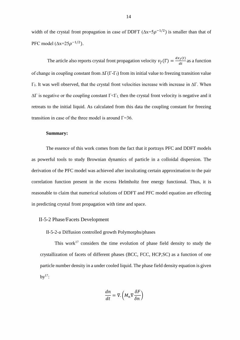
II-5-2-a Diffusion controlled growth Polymorphs/phases
This work17 considers the time evolution of phase field density to study the
crystallization of facets of different phases (BCC, FCC, HCP,SC) as a function of one
particle number density in a under cooled liquid. The phase field density equation is given
by17:
𝑑𝑛
𝑑𝑡= ∇. (𝑀𝑛∇
𝛿𝐹
𝛿𝑛 )
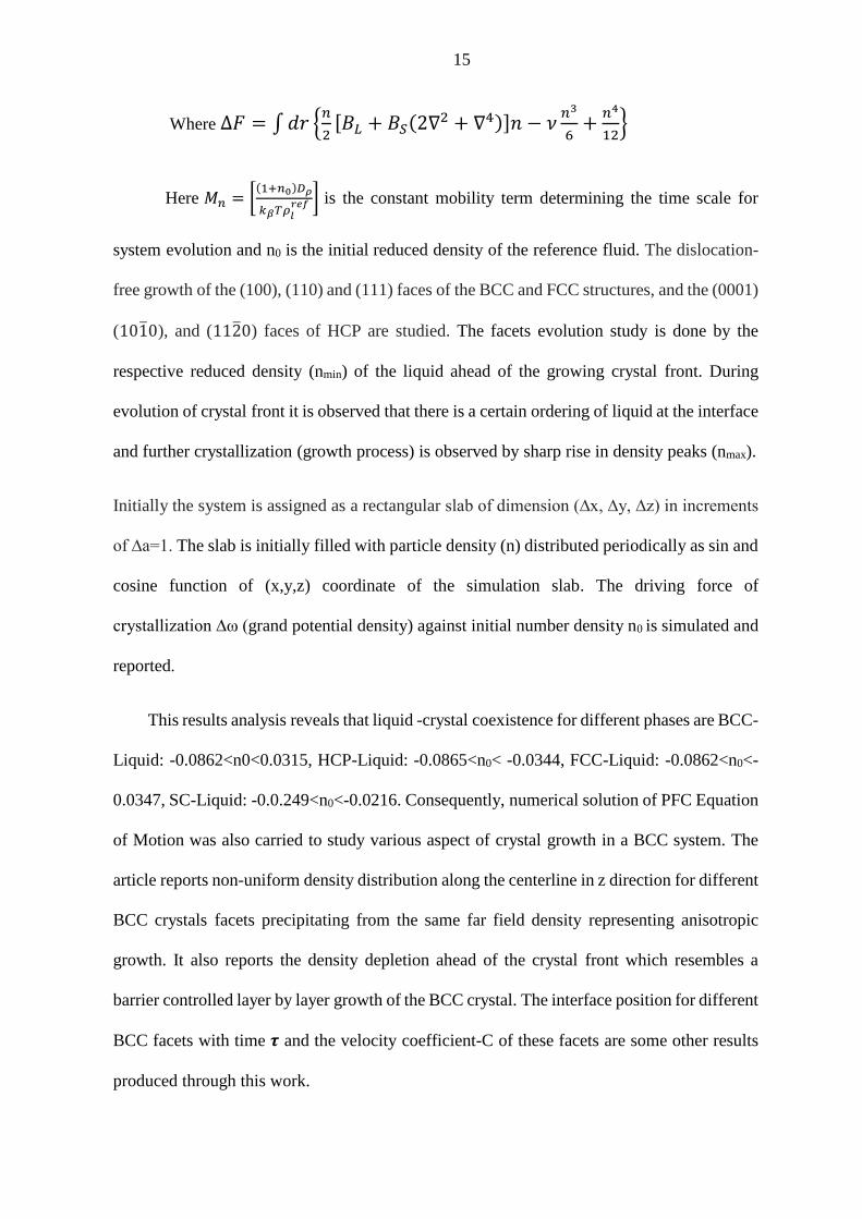
15
Where ∆𝐹 = ∫ 𝑑𝑟 {𝑛
2[𝐵𝐿 + 𝐵𝑆(2∇2 + ∇4)]𝑛 − 𝜈
𝑛3
6+
𝑛4
12}
Here 𝑀𝑛 = [(1+𝑛0)𝐷𝜌
𝑘𝛽𝑇𝜌𝑙𝑟𝑒𝑓 ] is the constant mobility term determining the time scale for
system evolution and n0 is the initial reduced density of the reference fluid. The dislocation-
free growth of the (100), (110) and (111) faces of the BCC and FCC structures, and the (0001)
(101̅0), and (112̅0) faces of HCP are studied. The facets evolution study is done by the
respective reduced density (nmin) of the liquid ahead of the growing crystal front. During
evolution of crystal front it is observed that there is a certain ordering of liquid at the interface
and further crystallization (growth process) is observed by sharp rise in density peaks (nmax).
Initially the system is assigned as a rectangular slab of dimension (∆x, ∆y, ∆z) in increments
of ∆a=1. The slab is initially filled with particle density (n) distributed periodically as sin and
cosine function of (x,y,z) coordinate of the simulation slab. The driving force of
crystallization ∆ω (grand potential density) against initial number density n0 is simulated and
reported.
This results analysis reveals that liquid -crystal coexistence for different phases are BCC-
Liquid: -0.0862<n0<0.0315, HCP-Liquid: -0.0865<n0< -0.0344, FCC-Liquid: -0.0862<n0<-
0.0347, SC-Liquid: -0.0.249<n0<-0.0216. Consequently, numerical solution of PFC Equation
of Motion was also carried to study various aspect of crystal growth in a BCC system. The
article reports non-uniform density distribution along the centerline in z direction for different
BCC crystals facets precipitating from the same far field density representing anisotropic
growth. It also reports the density depletion ahead of the crystal front which resembles a
barrier controlled layer by layer growth of the BCC crystal. The interface position for different
BCC facets with time 𝝉 and the velocity coefficient-C of these facets are some other results
produced through this work.

16
Summary:
The significance of this work is the fact that it was possible to predict the diffusion
controlled growth of a BCC, FCC and HCP crystal system coming from a surrounding liquid.
The phenomenon of diffusion controlled growth was supported by the fact that density
depletion zone between the liquid and crystal varies for different facets of a crystal system
(BCC as reported in this article). Moreover, the anisotropic growth in a BCC crystal system
was also reported in terms of plots of Interface position vs Time and Velocity coefficient vs
Initial Reduced Density(n0) for respective facets.
II-5-2-b Polymorphism & Crystal nucleation in PFC model in 2D and 3D
This work11,18 discusses about the thermodynamic driving force (minimization of free
energy) which result in the evolution different phases(BCC,FCC,HCP) in a homogenous
phase of given density. The equation of motion and Euler Lagrange (free energy minimization
with respect to Ψ) were solved numerically to study this phase evolution. These equations are
of the following form11
Euler Lagrange: 𝛿�̃�
𝛿𝛹=
𝛿�̃�
𝛿𝛹|𝛹0
(Ψ0 minimizes F)
Equation of motion: 𝑑𝛹′
𝑑𝑡= ∇̌2 {[𝑟∗′
+ (1 + ∇̌2)2
] 𝛹′ + 𝛹′3} + 𝛼∗
For the respective BCC, FCC, HCP phases the initial guess of the normalized
density(Ψ) was assigned as a combination of periodic sin and cosine function in space. On
computationally solving the equation of motion (density evolution) it was possible to predict
the equilibrium shape of the crystal whose faces are bounded by the planes of BCC, FCC and
HCP phases. In a different numerical analysis, the Euler Lagrange equation was solved to
predict a 3D phase diagram representing different phase with respect to reduced temperature
r* and reduced number density Ψ0. The three-phase equilibria (liquid–hcp–bcc, liquid–fcc–

17
hcp, hcp–bcc–rod, and fcc–hcp–rod) are represented by horizontal peritectic/eutectoid lines
in the phase diagram.
The other interesting results reported in this article is the 3-dimensional evolution of
equilibrium shapes for the FCC, BCC, HCP structures respectively. The equilibrium shapes
as predicted comes as rhombo-docodehdral, Octahedral and hexagonal prism structures
bounded by (100), (111) and (101̅0) planes for the respective BCC, FCC and HCP system.
The equilibrium crystal shapes whether BCC or FCC phase is determined after
observing the work of formation (grand canonical potential difference) against the number of
atoms.
Summary:
This work highlights the effective utilization of PFC model EOM and EL equations to
predict polymorphism and various aspect of crystal nucleation. The outcome of the simulation
was successful enough to predict a 3D phase diagram representing different phases i.e. Liquid-
FCC-HCP-BCC-Rod at different pair values of reduced temperature r*(contains information
about the physical properties of the model) and reduced number density Ψ0 with respect to
the reference fluid .The solution of the model reveals the final equilibrium shapes of the
nucleated crystals pertaining to BCC,FCC,HCP as rhombo-docodehdral ,Octahedral and
hexagonal prism structures bounded by (100),(111) and (101̅0) planes respectively.
II-5-2-c Heterogeneous Crystal Nucleation: The Effect of Lattice Mismatch
The objective of this work13,19 was to investigate the process of nucleation on a
crystalline substrate. The Helmholtz free energy density expression was modified to include
external potential Vext (r) of the substrate. The Helmholtz free energy expression here reads
as19:
18
∆𝐹 = ∫ 𝑑𝑟 {𝛹
2[∈ +(1 + ∇2)2]𝛹 + 𝑉𝑒𝑥𝑡(𝑟) +
𝛹4
4}
, where 𝛹 ∝𝜌−𝜌𝑟𝑒𝑓
𝜌 is the scaled density difference, ∈> 0 is the reduced temperature
related to the bulk moduli of the liquid and crystalline phase and is responsible for the
anisotropy in crystal growth. The effect of substrate is considered a s an external potential
whose properties are managed by the factor V(r). This factor which relates to the lattice
constant as and structure factor S(as,r) is added to the PFC Helmholtz free energy expression
to introduce the effect of substrate adsorption.
The dimensionless equations which were solved numerically pertaining to this work
includes ELE and EOM equation. They read as19:
Euler Lagrange Equation 𝛿𝐹
𝛿Ѱ= (
𝛿𝐹
𝛿Ѱ)
Ѱ0
(Ψ0 minimizes F)
Equation of motion 𝛿𝛹
𝛿𝜏= ∇2 𝛿𝐹
𝛿Ѱ+ 𝛼 , 𝛼 𝑏𝑒𝑖𝑛𝑔 𝑡ℎ𝑒 𝑔𝑎𝑢𝑠𝑠𝑖𝑎𝑛 𝑛𝑜𝑖𝑠𝑒
The Euler Lagrange equation was solved numerically at reduced temperature of ∈=
0.5 𝑎𝑛𝑑 ∈= 0.25 and varied lattice constant. The solution prescribes the development of
non-faceted parallel to a squared lattice wall for parameters ∈= 0.25, 𝛹0 = −0.341 and
𝑎𝑠
𝜎= 1.49 𝑎𝑛𝑑 2 respectively. However, with parameters ∈= 0.5, 𝛹0 = −0.514 and
𝑎𝑠
𝜎=
√3 𝑎𝑛𝑑 1 𝑟𝑒𝑠𝑝𝑒𝑐𝑡𝑖𝑣𝑒𝑙𝑦 faceted nuclei growth is observed.
The other phenomenon studied in this work is the growth of a nucleus on a cubic substrate.
The dimensions of the cubic substrate Ls are kept at 32 as and 16as , where as is the lattice
constant of a stable BCC structure. Iterative solution showed that with Ls=32as the growth on
the face of cube is spherical in nature whereas at Ls=16as the growth process comes as faceted
morphology.
19
Summary:
In this work the free energy equation of the PFC model was modified to include the
effect of external substrate. Thereafter these equations were solved numerically which showed
that the lattice mismatch between the substrate and crystal influence the growth morphology
of crystal. In addition, these results also convey the idea that the size of the foreign particle
effect the final growth morphology of crystal.
II-5-2-d Crystallization induced by multiple seeds: DDFT approach
In this work20 the process of crystallization was studied by introducing nucleating
seeds through an external potential 𝑉𝑝(𝑟) = ∑ 𝑉𝑝0𝑒−𝛼(𝑟−𝑟𝑖)2
𝑖 with parameters of the external
potential kept as 𝛼𝜎2 = 6 and 𝑉𝑝
0
𝑘𝑇= 4. To calculate dynamics of crystal growth the DDFT
equation was solved numerically which is given by20:
𝑑𝜌(𝑟, 𝑡)
𝑑𝑡= ∇ [𝜌(𝑟, 𝑡)
𝛿𝐹[𝜌(𝑟, 𝑡)]
𝜌(𝑟, 𝑡)]
With this approach, it was observed that the number of particle in each nucleus, the initial
orientation and area fraction play a part in grain boundary development between the growing
phases. In the first case when the area fraction of the external seeds was kept low the seeds
got dissolved and no net growth occurs. In case of an intermediate area fraction and small
orientation angle the resultant phase develops as a monocrystal. Finally, in the last case when
the orientation angle is large a crystal with grain boundary is formed.
The size ratio of the initial nuclei(N1/N2) is another factor which was assumed to play
a role in this exact phase behaviour. In the initial setup with N1=61 and N2=3, it was observed
that the boundary between the monocrystalline phase and the phase with grain shifts towards
smaller area fraction. This outcome can be interpreted as lower area fraction being sufficient
for the smaller size nucleus to remain stable. In the case when nuclei are kept smaller (N1 =
37 andN2 = 19), the phase boundary is strongly shifted to higher area fractions. It can be

20
inferred through this set of simulation results that at low area fractions the bigger nucleus
forms a more stable crystal—with larger density peaks and modifies the smaller crystal thus
finally filling the entire simulation box and hence no grain boundary or melting is observed.
Summary
In this work, it was successfully demonstrated that DDFT calculation were efficient
enough to study crystal growth on an externally imposed multiple nucleation seeds. These
results show that there are different scenarios when the initial nucleus grows into a fluid, a
monocrystal and crystal with grain boundary. The grain boundary formation and its final
position depends upon the size of the nuclei, the area fraction within the fluid and the initial
orientation of the seeds with respect to each other.
II-5-3 Morphology
II-5-3-a Tuning the structure of non-equilibrium soft materials by varying the
thermodynamic driving force for crystal ordering.
This work21 discusses the phenomenon of morphological change during crystallization
when the thermodynamic driving force are varied in a different set of simulation (Change in
particle concentration or level of under cooling of the liquid). The basic PFC equation of motion
was solved to study crystal growth on a nucleation seed introduced in a homogenous phase. The
Helmholtz free energy is given by21:
𝐹 = ∫ 𝑑𝑟 {𝛹
2[∈ +(1 + ∇2)2]𝛹 + +
𝛹4
4}
The Thermodynamic driving force depends upon:
Supersaturation: 𝑆 =𝛹0−𝛹𝐿
𝑒
𝛹𝑆𝑒−𝛹𝐿
𝑒 and Temperature: 𝝴
The crystal growth was studied for cases when effect of noise was pertinent (thermal
fluctuation) along with increase in supersaturation (varying 𝛹0).When the PFC model

21
equation of motion was solved including the thermal fluctuation the final shape crystal
morphology resulted as porous and irregular dendrite, whereas we see a more compact
hexagonal morphology when the thermal fluctuation was not included in the simulation.
The other part of this work compares the mechanism of the slow and the fast growth
mode (rate of change of supersaturation). The simulation results depict, that a slow growth
mode proceeds with evolution of faceted morphology, whereas in a fast growth mode non-
faceted morphology develops. Concurrently the simulation results showed that for a slow
growth process a sharp and faceted solid–liquid interface builds up at near-equilibrium,
whereas in a fast growth process a non-faceted interface builds up which extends to several
particle layers. The fast growth process was accompanied by a weak density depletion zone
which spread across the solid–liquid interface. The slow growth mode process is further
illustrated by simulation results which showed a narrow density depletion zone and a sharp
interface
It is claimed through these results that the diffusion mechanism which controls slow mode
allows more time to develop a faceted morphology (a sharp interface) unlike the kinetically
driven fast mode which results in uniform growth from all facets (interface between crystal
and liquid spreads towards many layer).
Conclusion
The results as conveyed and discussed in this work provides a theoretical description
to the understanding of crystal growth morphology at different mode. The analysis of these
results showed that slow mode of crystal growth is diffusion controlled by thermodynamics
whereas the fast mode is kinetically driven.

22
Chapter III-Results and Discussions
III-1 Experimental deduction
As stated in previous section the fundamental aim of this work is to analyse the
morphological phase transition behaviour of charge transfer complex material electro
crystallized on a substrate electrode. The experimental results as obtained through the course
of this work strongly supports the initial hypothesis of the work. Following the hypothesis,
K(def)TCP a charge transfer complex material was electro crystallized on a HOPG substrate
under varying condition of initial concentration and applied overpotential. To analyse the role
of these parameter on the morphology of electro crystallized K(def)TCP, Atomic force
microscopy imaging was performed post the electro crystallization process. The following
Atomic force microscopy images given in figure 1 ,2 ,3 depicts the electro crystallization
results under respective experimental condition.
Figure 1- Electrocrystallized K(def)TCP - Concentration: 0.05 M, Overpotential :1.2V and
Time of deposition: 1 second

23
Figure 2- Electrocrystallized K(def)TCP – Concentration:0.2 M, Overpotential:1.2V and Time
of deposition:1 second
Figure 3- Electrocrystallized K(def)TCP -Concentration:0.2 M, Overpotential: 1.5 V and Time
of deposition: 1 second

24
The experimental results as shown through the above-mentioned AFM images clearly
demonstrate that the morphology of electro crystallized K(def)TCP depends upon the initial
experimental parameters takes. The first of the cases (Figure 1) shows that at a low
concentration of 0.05M and a overpotential of 1.2 V, the morphology of the electro
crystallized K(def)TCP is preferably that of small spheres uniformly distributed along the
substrate. The morphological transition from spherical to small rod like structure (2nd case
AFM images) takes place when the K(def)TCP concentration was increased to 0.2 M under
the effect of same overpotential(1.2V) (Figure 2). Moreover, the rod like morphology of
K(def)TCP is more prominent when the overpotential is increased to 1.5V (Figure 3) and
K(def)TCP concentration is kept at 0.2M.
The outcome of the experimental work clearly builds up for the argument that
morphology of the deposited K(def)TCP on the substrate is driven by change in its initial
concentration and applied overpotential. Taking into perspective that the electro
crystallization process would be governed by the rates of diffusion or deposition of the
K(def)TCP atoms to the site on the substrate and that the two rates produce a net effect on the
morphology of deposited K(def)TCP on the substrate. Following on this analysis, it can be
argued that the electro crystallization process is thermodynamically driven when rate of
deposition lag that of diffusion, whereas kinetic takes over the thermodynamic of the process
in the reverse case scenario. Thus, the motivation arises implement Phase Field Crystal model
for our theoretical study whose inception comes from the basic concept classical
thermodynamics.
25
III-2 - Theoretical results
The Phase Field Crystal model is derived after making necessary approximation to the
Classical Density Functional model. The Helmholtz free energy functional in the PFC model
as derived and discussed in the previous chapter takes the following form11:
∆�̃� = ∫ 𝑑�̌� {𝛹
2[𝑟∗ + (1 + ∇̌2)
2] 𝛹 + 𝑡∗ 𝛹3
3+
𝛹4
4} (1)
The equation is dimensionless in Ψ which is the relative phase variable given by the
ratio of density difference between the one particle density of the crystal and a reference liquid
to the one particle density (𝜌−𝜌𝐿
𝑟𝑒𝑓)
𝜌. The variable 𝑟∗ is the model parameter incorporates the
effect of correlation coefficient (�̂�0, �̂�2 ) introduced after expanding the correlation function
�̂�𝐾 = �̂�0 + �̂�2𝑘2 + �̂�4𝑘4 in fourier space(k). At this point it’s a tangible fact that variable 𝑟∗
and the initial Ψ (reduced particle density) are two major properties which effect the phase
equilibrium between the periodic phase(Solid) and a homogenous phase(liquid) with time.
Having done a comprehensive review of the basics of the PFC model, it seemed relevant for
us to go ahead and investigate the direct correlation function 𝐶(𝑟, 𝑟′) from the view point of
classical thermodynamics.
III-2-a- Direct correlation function
To determine the direct correlation function for a system through a model present in
literature we referred to the Ornstein-Zernike Percus-Yevick (OZPY) equation22. The
OZPY is one of the most basic equation and is considered a good fit to generate the pair
correlation function of simple fluids interacting via Lennard Jones potential. It is of the
following form22:
𝑔(𝑟, 𝑟′) − 1 = 𝐶(𝑟, 𝑟′) + 𝑛 ∗ ∫ 𝐶(𝑟, 𝑟′) ∗ [𝑔(𝑟′′, 𝑟′) − 1]𝑑𝑟′′ -(2)

26
, where 𝑛 is the homogenous density distribution and thus is kept constant. The term
𝑘𝑇 is the thermal energy in terms of Boltzmann constant (k) and Temperature(T).
The Pair Correlation function 𝑔(𝑟, 𝑟′) in OZPY integral equation bears a linear
relationship with the direct correlation function 𝐶(𝑟, 𝑟′) along with an integral including the
interaction of a particle placed at 𝑟′′(𝑔(𝑟′′, 𝑟′)).The equation also incorporates the Percus-
Yevick approximation which correlates the pair correlation with the direct correlation
function is as follows22:
𝐶(𝑟, 𝑟′) = 𝑔(𝑟, 𝑟′) [1 − 𝑒𝑥𝑝𝑢(𝑟,𝑟′)
𝑘𝑇 ] (3)
, where 𝑢(𝑟, 𝑟′) is the potential (Lennard Jones (𝑟−6 − 𝑟−12)) acting between the
particles. We have performed our simulation run by choosing the units of 𝑢(𝑟, 𝑟′) in unit of
thermal energy (𝑘𝑇).
The OZPY equation is not in its simplest form because of the occurrence of 𝑔(𝑟, 𝑟′)
and 𝑔(𝑟′, 𝑟′′) which makes the solution of pair correlation function in Cartesian coordinates
unreasonable. Thus, follows the need to simplify the integral part of the OZPY equation in
polar coordinates (𝑟′′, 𝜃, 𝜑) which results in the following form of equation:
𝐼𝑛𝑡𝑒𝑔𝑟𝑎𝑙 =2𝜋
𝑟′∫ 𝑑𝑟′′𝑔(𝑟, 𝑟′′) ∫ 𝑟12𝑑𝑟12[𝑔(𝑟12) − 1]
𝑟"+𝑟′
|𝑟′′−𝑟′| (4)
Including the integral, the OZPY equation which we have numerically solved for the
direct correlation function
𝑦(𝑟, 𝑟′) = 1 + 𝑛 ∗2𝜋
𝑟′∫ 𝑑𝑟′′𝑔(𝑟, 𝑟′′) ∫ 𝑟12𝑑𝑟12[𝑔(𝑟12) − 1]
𝑟"+𝑟′
|𝑟′′−𝑟′| (5)
, where 𝑦(𝑟, 𝑟′) = 𝑔(𝑟, 𝑟′) ∗ 𝑒𝑥𝑝𝑢(𝑟,𝑟′)
𝑘𝑇

27
Figure 4 is the plot of the pair correlation function g (r, r’) at a reduced temperature of
2(𝑢(𝑟, 𝑟′) in units of thermal energy (𝑘𝑇)). The graph gives the plot of the pair correlation
function for two different values of homogenous density 𝑛 in the OZPY equation. The effect
of high homogenous density 𝑛 is evident from the red curve compared to that of low
homogenous density given by green curve. The simulation results presented here are at a
reduced temperature of (𝛽 =1
𝑘𝑇) 2 and homogenous density of 0.55 and 0.25.
The pair correlation plot in figure 4 is evidence of the fact that the initial homogenous
density of the liquid influences the pair correlation and the arrangement of atoms around a
reference atom. The red curve represents the case of a higher density homogenous phase
(0.55) and have two peaks showing higher packing of atoms. On the other case the green
curve with a lower initial density distribution has only one prominent peak implying lesser
correlation/packing among atoms.
Figure 4- Pair Correlation function for Homogenous density 0.55 (red curve) and 0.25 (green
curve).
From here onwards, we refer back to the percus-Yevick relation (equation 2) to compute
the direct correlation function (𝐶(𝑟, 𝑟′) from the pair correlation function (𝑔(𝑟, 𝑟′).At this point

28
we may go forward and expand the direct correlation in Fourier space as �̂�𝐾 = �̂�0 + �̂�2𝑘2 +
�̂�4𝑘4 and calculate r* parameter of the PFC model from these coefficient. This facilitates the
use of the PFC model to study the phase behaviour (Ψ) for a fluid or an ideal gas interacting via
Lennard Jones potential. However due to the unknown nature of the interacting potential between
atoms/ions in solid and periodic phases the solution of direct correlation function though this
method becomes trivial and unthinkable. Considering this problem, it is usually recommended
to use a numerical value of r*(sometime referred to as reduced temperature) as an initial guess
which is close enough to the physical properties (compressibility, Bulk modulus) of the
material/phase to be studied through the model. In the next section, we will discuss some of the
results we have produced on solving the equation of motion of the PFC model in 1 dimension.
III-2-b Equation of motion
In the previous section, we have discussed the Helmholtz free energy functional
(equation 1) of the PFC model. However, the free energy equation that we have simulated in
this work is modified to the simplest form possible. For instance we have solved the equation
of motion without considering the multiplier 𝑡∗as it accounts for the complex contribution of
three particle correlation 11 .Moreover we have solved the PFC equation of motion on the
standard length scale(x) rather than the scale �̂� =2∗(
𝐶4𝐶2
)
12
𝑥 (corresponds to the maximum of
correlation function) on which the Helmholtz free energy of the conventional PFC model has
been derived .Incorporating these modification the expression for the Helmholtz free energy
we arrive to is given by:
∆𝐹 = ∫ 𝑑𝑟 {𝛹
2[𝑟∗ + (1 + ∇2)2]𝛹 +
𝛹4
4}
The corresponding equation of motion to this form of Helmholtz free energy thus
takes the following form:

29
𝑑𝛹
𝑑𝑡= ∇2{[𝑟∗ + (1 + ∇2)2]𝛹 + 𝛹3} (6)
Equation 6 is a sixth order differential equation which needs a set iterative method to
solve over time. To solve the equation in one dimension we have implemented forward Euler
Scheme (finite difference) where each iterative step is as follows
𝛹𝑡+∆𝑡,𝑛 = 𝛹𝑡,𝑛 + ∆𝑡 ∗ ∇2{[𝑟∗ + (1 + ∇2)2]𝛹 + 𝛹3}
The Laplacian and higher order differential in the equation are solve based on finite
difference scheme and Discrete Fourier Transform algorithm. As Per the finite difference
scheme the Laplacian of the phase variable Ψ at any x position in space and time t is given by
𝜕2 𝛹
𝜕𝑥2=
𝛹𝑡,𝑥−∆𝑥 + 2 ∗ 𝛹𝑡,𝑥 + 𝛹𝑡,𝑥+∆𝑥
(∆𝑥)2
We have solved the equation of motion by plugging in an initial distribution of Ψ
along space and value of r* in equation of motion.
Figure 5- Random distribution of Ψ at Time =0

30
Figure 5 represents the distribution in space where phase variable Ψ is initialized as
random fluctuation around zero resembling initial perturbation in a homogenous liquid. The
space variable is discretized as ∆x=0.4. The value of r*(reduced temperature) chosen is 0.4
for this case and the simulation is run for 20 units of time at an increment of 0.0001. Figure 6
gives the distribution of Ψ at Time=20.The boundary condition are taken periodic in nature.
As is can be observed from Figure 6 Ψ has changed from a random fluctuation to a more
periodic phase. This behaviour can be inferred as an effect of sudden undercooling of the
liquid by the factor r*=-0.4 in space which results from a random fluctuation into a periodic
ordered phase. Our simulation results and the reasoning that follows it seems coherent with
the physical mechanism behind the liquid-solid transition in a solidification process.
Figure 6- Periodic phase distribution of Ψ at Time =20
We next fitted the periodic phase distribution of figure 6 to a Sin function of the form
𝐴𝑠𝑖𝑛(𝑘𝑥 − 𝑥0) ,with k as the wavenumber. On number of trial we found that 0.6 ∗ sin (1.1𝑥)
best fit the periodic phase distribution at r*=-0.4;

31
The results observed in Figure 6 after iteratively solving the PFC equation of motion with
initial parameters shows the utility of the model to study transition between two phases
(random to periodic) with time. As discussed above we fitted this periodic phase to a Sin
function of the form 𝐴𝑠𝑖𝑛(𝑘𝑥 − 𝑥0) and could obtain reasonable results. For our next case,
we believed that it was necessary to study the effect of change of model parameters on the
phase transition behaviour. On that note we ran few other simulations by placing a crystal in
a homogenous phase of reduced density 𝛹0.For that purpose Ψ was initialized as a periodic
phase of the form ( 𝐴 ∗ sin(𝑘𝑥) + 𝛹0) for certain portion in space. We initialized the wave
number k as 1. The simulation run was performed for different pair of r* and 𝛹0.Figure 8 and
9 gives the simulation results at time t=0 and t=10 for the case with 𝛹 taken initially as 0.72 ∗
𝑠𝑖𝑛(𝑥) + 0.45 .
Figure 7- Ψ obtained from initial random fluctuation fitted with a periodic function at r*=-0.4

32
Figure 8- Placing a crystal with periodicity Ψ=0.72*sin(x)+0.45 in a homogenous phase at time
t=0 and driving force for solidification given by r*=-0.2
Figure 8 and 9 shows the phase transition Ψ from t=0 to t=10 at the initial quench
given by r*= -0.2. The crystal with periodicity Ψ=0.72*sin(x)+0.45 placed in the homogenous
phase disappears and cease to grow at this value of quench(r*=-0.2) parameter and reduced
particle density 𝛹0 = 0.45.
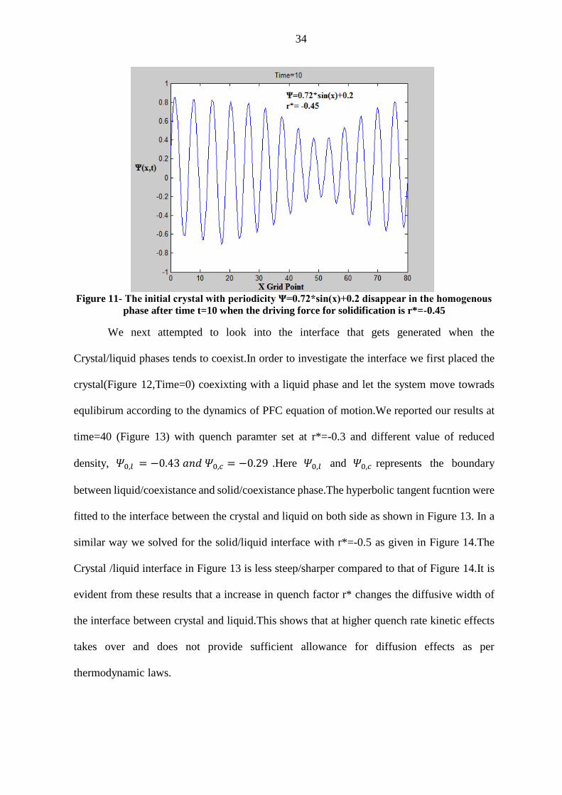
We next considered a different pair of value for 𝛹0 and r*.Figure 10 and 11 gives the
simulation results at time t=0 and t=10 respectively. The value assigned to 𝛹0 and r* in this
case are 0.2 and -0.45. Figure 10 resembles a crystal with perodicity Ψ=0.72*sin(x)+0.2
placed in a homogenous phase with reduced density (𝛹0 ) 0.2. As is evident from the result
given in Figure 11 the crystal has fully grown across the interface crystal/liquid by time t=10.
The simulation results as shown in Figure 9 and 11 are of extreme relevance to determine
equilibrium existence or coexistence of crystal/liquid phase along the independent variation
of quench parameter(r*) and reduced particle density (𝛹0 ).These results holds good to

33
predict the liquid-crystal phase transition from inherent material properties given by r* and
the homogenous phase(with reduced density 𝛹0) surrounding it.
Figure 9- Crystal placed in liquid disappears at time t=10 when the parameter r*=-0.2
Figure 10- Placing a crystal with periodicity Ψ=0.72*sin(x)+0.2 in a homogenous phase at time
t=0 and driving force for solidification given by r*=-0.45
34
Figure 11- The initial crystal with periodicity Ψ=0.72*sin(x)+0.2 disappear in the homogenous
phase after time t=10 when the driving force for solidification is r*=-0.45
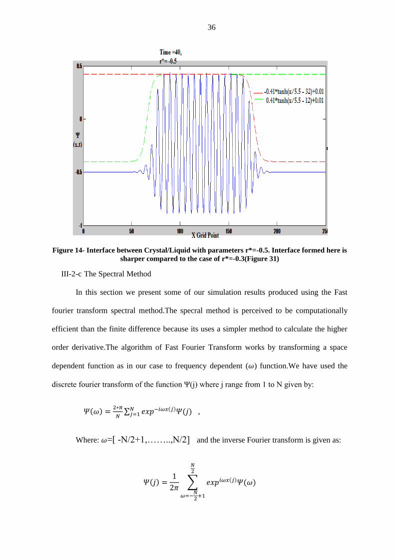
We next attempted to look into the interface that gets generated when the
Crystal/liquid phases tends to coexist.In order to investigate the interface we first placed the
crystal(Figure 12,Time=0) coexixting with a liquid phase and let the system move towrads
equlibirum according to the dynamics of PFC equation of motion.We reported our results at
time=40 (Figure 13) with quench paramter set at r*=-0.3 and different value of reduced
density, 𝛹0,𝑙 = −0.43 𝑎𝑛𝑑 𝛹0,𝑐 = −0.29 .Here 𝛹0,𝑙 and 𝛹0,𝑐 represents the boundary
between liquid/coexistance and solid/coexistance phase.The hyperbolic tangent fucntion were
fitted to the interface between the crystal and liquid on both side as shown in Figure 13. In a
similar way we solved for the solid/liquid interface with r*=-0.5 as given in Figure 14.The
Crystal /liquid interface in Figure 13 is less steep/sharper compared to that of Figure 14.It is
evident from these results that a increase in quench factor r* changes the diffusive width of
the interface between crystal and liquid.This shows that at higher quench rate kinetic effects
takes over and does not provide sufficient allowance for diffusion effects as per
thermodynamic laws.

35
Figure 12- Crystal placed in a liquid at time =0.
Figure 13- Interface between Crystal/Liquid with parameters r*=-0.3
36
Figure 14- Interface between Crystal/Liquid with parameters r*=-0.5. Interface formed here is
sharper compared to the case of r*=-0.3(Figure 31)
III-2-c The Spectral Method
In this section we present some of our simulation results produced using the Fast
fourier transform spectral method.The specral method is perceived to be computationally
efficient than the finite difference because its uses a simpler method to calculate the higher
order derivative.The algorithm of Fast Fourier Transform works by transforming a space
dependent function as in our case to frequency dependent (𝜔) function.We have used the
discrete fourier transform of the function Ψ(j) where j range from 1 to N given by:
𝛹(𝜔) =2∗𝜋
𝑁∑ 𝑒𝑥𝑝−𝑖𝜔𝑥(𝑗)𝛹(𝑗)𝑁
𝑗=1 ,
Where: 𝜔=[ -N/2+1,……..,N/2] and the inverse Fourier transform is given as:
𝛹(𝑗) =1
2𝜋∑ 𝑒𝑥𝑝𝑖𝜔𝑥(𝑗)𝛹(𝜔)
𝑁2
𝜔=−𝑁2
+1

37
If Ψ(j) is Fourier transformed as 𝛹 ̂(ω) then the Fourier transform of higher order
derivative of Ψ(j) bears the following relation with
Ƒ[ 𝛻2𝛹(𝑗)] = −𝜔2�̂�(𝜔)
Ƒ[ 𝛻2𝛹(𝑗)] = 𝜔4�̂�(𝜔)
Incorporating these relations makes Helmholtz free energy functional of the PFC
model looks like
𝑑�̂�
𝑑𝑡= −𝜔2(𝑟 ∗ +(1 − 𝜔2)2)�̂� − 𝜔2𝛹3̂ (7)
The above equation contains a linear and nonlinear term(𝛹3̂) .Thus we need to
operator split the above equation i.e we solve the linear and non linear part separately and
then merge the invidual results afterwards. Therefore we solve the linear and non linear part
of differential equation separately and apply the forward Euler scheme which results in a
numerical solution of the form
�̂�(𝑡 + ∆𝑡) = �̂�(𝑡)𝑒𝑥𝑝𝐿𝜔∆𝑡 − ∆𝑡𝑘2𝛹3̂ (8)
Where 𝐿𝜔 = −𝜔2(𝑟 ∗ +(1 − 𝜔2)2)
The vector 𝜔 in this instance is the fourier space frequency variable given by
𝜔 = [0, ∆𝜔, 2∆𝜔, … . .𝜋
∆𝑥, −
𝜋
∆𝑥+ ∆𝜔, −
𝜋
∆𝑥+ 2∆𝜔,…-∆𝜔]
Here ∆𝜔 =2𝜋
𝑁∆𝑥, N being the size of the vector in x space.
We ran our simulation on equation (8) iteratively over time .In each of the simulation
we descritized space variable ∆x=0.1 and time ∆t=0.0001.The system size in real space range
from x=-400 to 400. The utility of fourier transform alogorithm in simplifying the higher order

38
derivative gives us an edge to solve the PFC equation of motion for a larger size system and
higher computational speed.Figure 15 gives the simulation results of equation 8 with quench
factor r*=-0.7 at time =35.For comparative analysis of this result we performed similar
simulation on equaiton 8 with quench factor r*=-0.2 at time =35.
The solution of the PFC equation of motion given in Figure 15 and 16 shows that the
quench paramter r* determines the crystal propogation.A higher value of r* accounts for the
crystal front propagating to larger length than a lower r*.This deduction falls in line with our
earlier analysis made through finite difference alogorithm.
Figure 15- Propagating crystal front at r*=-0.7. The figure only shows the right side of the
crystal
.

39
Figure 16- Propagating crystal front at r*=-0.2. The figure only shows the right side of the
crystal

40
Chapter IV-Conclusion
In this work, we have tried putting up a sincere effort to analyse the phase transition
behaviour during a crystallization process. The analysis of the experimental results on electro
crystallized charge transfer complex material on a substrate electrode laid the initial
foundation of our research. The morphological transition of these charge transfer complex
materials under different condition of concentration and applied overpotential were relevant
results to adopt phase field crystal model(PFC) for our theoretical work. The phase field
crystal(PFC) is an effective model to study the equilibrium between a homogenous(liquid)
and a periodic phase(crystal). The equilibrium state of the system in a PFC model is
represented in terms of Helmholtz free energy functional of density profile. The relation
between the change in density profile with time and the proportional change in the Helmholtz
free energy with respect to this density profile is referred to as the PFC equation of motion.
We have solved the PFC equation of motion for different parameters and have achieved
decent quantitative results. We have argued through our results that growth or disappearance
of a periodic phase in a homogenous phase depends upon the initial parameters r* and Ψ0. We
have also determined the nature of interface region between coexisting phases through our
simulations. We have performed these simulations using the finite difference and Fast Fourier
transform algorithm. We have realized through our analysis that the implementation of Fast
Fourier Transform significantly increases the computational speed and allows simulation of
large system than with the finite difference scheme. These results are encouraging to claim
that the PFC model is a powerful tool to correlate with the real time behaviour during a
crystallization process.

41
Chapter V-Future work
The results and data reported in this thesis holds significance for further study of the
phase transition phenomenon during the process of crystallization. We have structured our
research based on the preliminary demonstration of phase transition behaviour of charge
transfer complex material subjected to electro crystallized on a substrate electrode. These
results laid initial ground work to adopt the well-known Phase field crystal(PFC) model for
our theoretical study. The simulation results of this work are concrete evidence of the point
that PFC model is a powerful tool to investigate research problems related to the
crystallization process. We have used the most fundamental PFC model for our work in which
the driving force for transition between a periodic and homogenous phase depends solely on
quench parameter r* and reduced particle density. However, the interaction of charged species
in an electro crystallization process it requires necessary modification of the PFC model
currently implemented in this work. Moreover, we have restricted the PFC model simulation
to 1 dimensional system and have left sufficient space to implement the model to higher
dimensions. Our simulation results are encouraging and are a step in the direction to consider
PFC for enhanced theoretical study of crystallization process. In a future study, the excess
Helmholtz free energy functional of classical density functional theory containing the direct
correlation function will change to incorporate the electrostatic interaction among particles.
It is worth mentioning that there have been successful attempts to use a modified form of the
original CDFT23 in systems with charged hard sphere24,25, asymmetric electrolyte26
.Therefore, a new form of PFC model derived from these modified CDFT model will certainly
alleviate the understanding of electro crystallization process on a larger scale..

42
APPENDIX
Matlab code solving PFC using Finite difference
clc clear all dr=0.4; x=0:dr:40; dr2=dr^2; m=zeros(1,length(x)); Si=-0.2+0.4*rand(1,length(x)); % Si taken as initial random
distribution
f1=figure; plot(x,Si); % Plotting Si at time=0 axis([0 40 -1.5 1.5]) title('Time = 0'); f2=figure; t=50; dt=0.0001; epsilon=0.2;
for i=0:dt:t Si3=Si.^3; % Si^3 calculated from Si Si_old=Si; % Current Si for j=1:length(Si) cnt=j+1; cnt1=j-1;
if (cnt==length(Si)+1) cnt=1; % applying periodic boundary condition to Si end if (cnt1==0) cnt1=length(Si); % applying periodic boundary condition to
Si end term1(j)=(Si(cnt)-2*Si(j)+Si(cnt1))/(dr2); % Taking Laplcian of
Si at each grip point term4(j)=(Si3(cnt)-2*Si3(j)+Si3(cnt1))/(dr2); % Taking
Laplacian of Si^3 at each grid point end for k=1:length(term1) cnt2=k+1; cnt3=k-1; if (cnt2==length(term1)+1) cnt2=1; % applying periodic boundary condition to
laplacian of Si end if (cnt3==0) cnt3=length(term1); % applying periodic boundary condition
to laplacian of Si end term3(k)=(term1(cnt2)-2*term1(k)+term1(cnt3))/(dr2);% Taking
Laplacian^2 of Si at each grid point end for l=1:length(term3) cnt4=l+1; cnt5=l-1;
43
if (cnt4==length(term3)+1) cnt4=1; % applying periodic boundary condition
to laplacian^2 of Si end if (cnt5==0) cnt5=length(term3); % applying periodic boundary condition
to laplacian^2 Si end term2(l)=(term3(cnt4)-2*term3(l)+term3(cnt5))/(dr2); % Taking
Laplacian^4 at each grid point end grad_Si=((1-epsilon)*term1+term2+2*term3+term4)*dt; % change
in Si after time dt Si=Si_old+grad_Si; % Si at time t+dt if(rem(i,1000*dt)==0) figure(f2) plot(x,Si) % Plotting Si after 1000dt axis([0 40 -1 1]) title(['Time=' num2str(i)]); pause(0.0001) end end
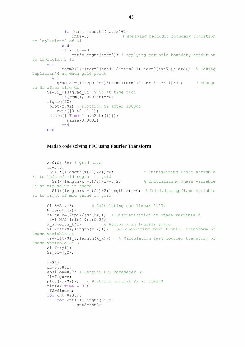
Matlab code solving PFC using Fourier Transform
x=0:dr:80; % grid size
dr=0.5; Si(1:((length(x)+1)/2))=0; % Initializing Phase variable
Si to left of mid region in grid Si(((length(x)+1)/2)+1)=0.2; % Initializing Phase variable
Si at mid value in space Si(((length(x)+1)/2)+2:length(x))=0; % Initializing Phase variable
Si to right of mid value in grid
Si_3=Si.^3; % Calculating non linear Si^3. N=length(x); delta_k=(2*pi)/(N*(dr)); % Discretization of Space variable k z=[-N/2+1:1:0 0:1:N/2]; k_x=delta_k*z; % Vector k in fourier space y1=(fft(Si,length(k_x))); % Calculating fast fourier transform of
Phase variable Si y2=(fft(Si_3,length(k_x))); % Calculating fast fourier transform of
Phase variable Si^3 Si_f=(y1); Si_3f=(y2);
t=35; dt=0.0001; epsilon=0.7; % Setting PFC parameter Si f1=figure; plot(x,(Si)); % Plotting initial Si at time=0 title('Time = 0'); f2=figure; for cnt=0:dt:t for cnt1=1:length(Si_f) cnt2=cnt1;

44
term1(cnt1)=(-((k_x(cnt2))^2)*(-epsilon+(1-
(k_x(cnt2))^2)^2))*dt; % Converting PFC equation of motion differential
equation as per fourier transformation
grad_Si_f(cnt1)=Si_f(cnt2)*exp((term1(cnt1))); % calculating
gradient of fourier of Si. grad_Si_3f(cnt1)=(-(Si_3f(cnt2))*(((k_x(cnt2))^2))*dt); %
calculating gradient of fourier of Si^3. end
Si_f=(grad_Si_f+grad_Si_3f); % Si in fourier space at t+dt Si=(ifft(Si_f,length(k_x))); % Taking Si back to real space
Si_3=Si.^3; % Updating Si^3 from new Si Si_3f=(fft(Si_3,length(k_x))); % Updating fourier transform of Si^3 if(rem(cnt,1000*dt)==0) figure(f2) Si_new=Si((length(x)+1)/2:length(x)); % Considering phase
variable Si after 1000*dt x1=x((length(x)+1)/2):dr:x(length(x)); plot(x1,Si_new) % Ploting Si after 1000dt
title(['Time' num2str(cnt)]); pause(0.0001) end end

45
REFERENCES
(1) Li, L.; Jahanian, P.; Mao, G. J. Phys. Chem. C 2014, 118, 18771–18782.
(2) Kahl, G.; Löwen, H. J. Physics: Condens. Matter 2009, 21.
(3) Neuhaus, T.; Härtel, A.; Marechal, M.; Schmiedeberg, M.; Löwen, H. Eur.
Phys. J. Spec. Top. 2014, 223, 373–387.
(4) Cacciuto, A.; Auer, S.; Frenkel, D. Nature 2004, 428, 404–406.
(5) Emmerich, H.; Löwen, H.; Wittkowski, R.; Gruhn, T.; Tóth, G. I.; Tegze, G.;
Gránásy, L. Adv. Phys. 2012, 61, 665–743.
(6) Ramakrishnan, T. V.; Yussouff, M. Phys. Rev. B 1979, 19, 2775–2794.
(7) Likos, C. N.; Mladek, B. M.; Gottwald, D.; Kahl, G. J. Chem. Phys. 2007, 126,
224502.
(8) Donev, A.; Vanden-Eijnden, E. J. Chem. Phys. 2014, 140, 234115.
(9) Smoluchowski, M. V. Ann. Phys. 1916, 353, 1103–1112.
(10) Podmaniczky, F.; GI Tóth, G. T., T. Pusztai…. J. Cryst. Growth 2016.
(11) Tóth, G. I.; Tegze, G.; Pusztai, T.; Tóth, G.; Gránásy, L. J. Physics: Condens.
Matter 2010, 22.
(12) Alster, E.; Elder, K. R.; Hoyt, J. J.; Voorhees, P. W. Phys. Rev. 2017, 95.
(13) Podmaniczky, F.; Tóth, G. I.; Tegze, G.; Gránásy, L. Metall. Mater. Trans.
2015, 46, 4908–4920.
(14) Ofori-Opoku, N.; Stolle, J.; Huang, Z.-F.; Provatas, N. Phys. Rev. B 2013, 88.
(15) Van Teeffelen, S.; Likos, C. N.; Löwen, H. Phys. Rev. Lett. 2008, 100.
(16) Van Teeffelen, S.; Backofen, R.; Voigt, A.; Löwen, H. Phys. Rev. 2009, 79.
(17) Tegze, G.; Gránásy, L.; Tóth, G. I.; Podmaniczky, F.; Jaatinen, A.; Ala-Nissila,
T.; Pusztai, T. Phys. Rev. Lett. 2009, 103.

46
(18) Gránásy, L.; Podmaniczky, F.; Tóth, G. I.; Tegze, G.; Pusztai, T. Chem. Soc.
Rev. 2014, 43, 2159–2173.
(19) Tóth, G. I.; Tegze, G.; Pusztai, T.; Gránásy, L. Phys. Rev. Lett. 2012, 108.
(20) Neuhaus, T.; Schmiedeberg, M.; Löwen, H. Phys. Rev. 2013, 88.
(21) Tegze, G.; Gránásy, L.; Tóth, G. I.; Douglas, J. F.; Pusztai, T. Soft Matter 2011,
7, 1789–1799.
(22) Wang, Q.; Keffer, D. J.; Nicholson, D. M.; Thomas, J. B. Phys. Rev. 2010, 81.
(23) Knepley, M. G.; Karpeev, D. A.; Davidovits, S.; Eisenberg, R. S.; Gillespie,
D. J. Chem. Phys. 2010, 132, 124101.
(24) Gillespie, D.; Nonner, W.; Eisenberg, R. S. Phys. Rev. 2003, 68.
(25) Rosenfeld, Y. J. Chem. Phys. 1993, 98, 8126.
(26) Li, Z.; Wu, J. Phys. Rev. 2004, 70.

47
ABSTRACT
ENGINEERING CRYSTALLIZATION via PHASE FIELD
CRYSTAL MODEL
Advisor: Dr. Korosh Torabi
Major : Material Science and Engineering
Degree: Master of Science
Charge transfer complex material demonstrate morphological transitions while electro-
crystallized on a substrate electrode under varying solute concentration and applied
overpotential. It is hypothesized that variations in these parameters affect the thermodynamics
and the kinetics of the electro-crystallization process. Having analysed these results, we resort
to applying phase field crystal(PFC) model for our theoretical study. Our initial literature
review laid foundation to consider PFC model as a powerful tool to study various aspect of
crystallization process. In a PFC model the thermodynamic state of a system under study is
defined in terms of Helmholtz free energy functional of density profile 𝐹 = 𝐹[𝜌(𝑟)].Our
numerical solution of the time-dependent PFC model demonstrates that the phase transition
behaviour between a periodic crystal phase and a homogenous phase can be tuned by
changing parameters within the PFC equation. These simulations also predicted the nature of
the interface between solid/liquid phase at different simulation conditions. Moreover, it was
evident from our results that solution of the PFC equation of motion through Fast Fourier
Transform algorithm is computationally faster which facilitates the simulation of a large
system.

48
Autobiographical Statement
Following my deep interest in the field of Material science and Engineering I was motivated
to pursue my master’s studies in this major at Wayne State University, Detroit United States.
It was during the initial phase of regular coursework in this major I was introduced to the tool
of modelling and simulation applied to various area of research. In particular I was deeply
impressed with the concepts of statistical mechanics and advanced thermodynamics applied
to research problems at microscopic level. On realizing my new found interest in the
application of Modelling and Simulation techniques to fundamental research topic, I choose
to work under the supervision Dr Korosh Torabi, Asst Prof Department of Chemical and
Material science Engineering at Wayne State University for my Masters degree thesis work.
I was fortunate to have reached out to him at a time when he had just started working on a
collaborated research work with Dr Guangzhao Mao experimental group on a project outlined
as the “Engineering the morphology of electro crystallization kinetics of organic nanorods on
a substrate “.On Dr Torabi recommendation I was lean towards undertaking this research via
experimental and theoretical route. The experimental part of my research work involves
electrocrystallization of charge transfer complex TTFBr nanorods on a selectively oriented
substrate followed up by morphological analysis via Atomic force microscopy imaging.
Moreover, on the theoretical front I am involved in investigating previous literature work
conducted via utilizing Phase field crystal thermodynamic model derived from the concepts
of Classical density functional theory towards studying phase transition of materials on a
substrate. On a final note I once again wants to give my sincere regards to Dr Torabi for his
immense support and valuable guidance in letting me explore and build my foundation in
areas from the point of view of statistical mechanics and Classical Thermodynamics.
Top Related