


Languages
Pages
Legal


Ellipsometry in Interface Science
H. Motschmann and R. Teppner
Max-Planck-Institut fur Grenzflachenforschung, Golm
Contents
1 What is it all about? 2
2 Polarized light 2
3 Basic equation of ellipsometry 5
4 Design of an ellipsometer 6
5 Theory of reflection 10
6 Ellipsometry applied to ultrathin films 17
7 Microscopic model for reflection 19
8 Adsorption layers of soluble surfactants 23
8.1 Importance of purification . . . . . . . . . . . . . . . . . . . . . . . . . . . 23
8.2 Physicochemical properties of our model systems . . . . . . . . . . . . . . 23
8.3 Adsorption layer of a nonionic surfactant . . . . . . . . . . . . . . . . . . . 24
8.4 Ionic surfactant at the air-water interface . . . . . . . . . . . . . . . . . . . 25
8.5 Kinetics of absorption . . . . . . . . . . . . . . . . . . . . . . . . . . . . . 34
9 Principle of imaging ellipsometry 36
9.1 Depth of field problem . . . . . . . . . . . . . . . . . . . . . . . . . . . . . 37
9.2 Beyond the diffraction limit . . . . . . . . . . . . . . . . . . . . . . . . . . 39

2
1 What is it all about?
The following chapter presents the basics of ellipsometry and discusses some recent ad-
vances. The article covers the formalism and theory used for data analysis as well as
instrumentation. The treatment is also designed to familiarize newcomers to this field.
The experimental focus is on adsorption layers at the air-water and oil-water interface.
Selected examples are discussed to illustrate the potential as well as the limits of this
technique. The authors hope, that this article contributes to a wider use of this technique
in the colloidal physics and chemistry community. Many problems in our field of science
can be tackled with this technique.
Ellipsometry refers to a class of optical experiments which measure changes in the state
of polarization upon reflection or transmission on the sample of interest. It is a powerful
technique for the characterization of thin films and surfaces. In favorable cases thicknesses
of thin films can be measured to within A accuracy, furthermore it is possible to quantify
submonolayer surface coverages with a resolution down to 1/100 of a monolayer or to
measure the orientation adopted by the molecules on mesoscopic length scales. The high
sensitivity is remarkable if one considers that the wavelength of the probing light is on
the order of 500 nm. The data accumulation is fast and allows to monitor the kinetics of
adsorption processes. The technique can also be extended to a microscopy. Imaging ellip-
sometry allows under certain conditions a direct visualization of surface inhomogeneities
as well as quantification of the images. Many samples are suitable for ellipsometry and
the only requirement is that they must reflect laser light. Its simplicity and power makes
ellipsometry an ideal surface analytical tool for many objects in interface science.
2 Polarized light
Light is an electromagnetic wave and all its features relevant for ellipsometry can be
described within the framework of Maxwell’s theory [1]. The relevant material properties
are described by the complex dielectric function ε or alternatively by the corresponding
refractive index n.

3
An electromagnetic wave consists of an electric field ~E and a magnetic field ~B. The field
vectors are mutually perpendicular and also perpendicular to the propagation direction
as given by the wave vector ~k. All states of polarization are classified according to the
trace of the electrical field vector during one period. Linearly polarized light means the
electrical field vector oscillates within a plane, elliptically polarized light means that the
trace of the electric field vector during one period is an ellipse. A convenient mathematical
representation of a given state of polarization is based on a superposition of two linearly
polarized light waves within an arbitrarily chosen orthogonal coordinate system.
~E(~r, t) =
|Ep| cos(2πνt− ~k · ~r + δp)
|Es| cos(2πνt− ~k · ~r + δs)
(1)
|Ep| and |Es| are the amplitudes, δp and δs the phases, |~k| = 2π/λ is the magnitude of the
wave vector and ν the frequency. Only the phases δp, δs and the amplitudes are required
for a representation of the state of polarization; the time dependence is not of importance
and can be neglected. The so called Jones vector reads
~E =
|Ep|eiδp
|Es|eiδs
=
Ep
Es
(2)
Different states of polarization are depicted in Fig. 1. The state of polarization is
a) linear, if δp − δs = 0 or δp − δs = π,
b) elliptical, if δp 6= δs and |Ep| 6= |Es|,
c) circular for the special case δp − δs = π/2 and |Ep| = |Es|.
handedleft handed right
Phase shift
0
7λ/8
3λ/4
3λ/85λ/8
λ/4
λ/2
λ/8
S
P
Figure 1: The Jones representation of polarized light represents any state of polarization as a linear
combination of two orthogonal linearly polarized light waves.

4
An alternative representation of a given state of polarization uses the quantities ellipticity
ω and azimuth α. The ellipticity is defined as the ratio of the length of the semi-minor
axis to that of the semi-major axis as shown in Fig. 2. The azimuth angle α is measured
counterclockwise from the Ýx-axis. Light is assumed to propagate in positive Ýz direction
so that Ýx, Ýy and Ýz define a right handed coordinate system. Some authors prefer this
representation and for this reason the conversion formulas between both notations are
listed below. The derivations require a vast number of tedious algebraic manipulations
and can be found in [2].
tan 2α =2ExEycos(δy − δx)
E2x − E2
y
− 90 ≤ α ≤ 90 (3)
sin(2ω) =2ExEy sin(δy − δx)
E2x + E2
y
− 45 ≤ ω ≤ 45 (4)
tan(δy − δx) =tan(2ω)
sin(2α)− 180 ≤ δy − δx ≤ 180 (5)
cos
(
2 arctan
(
Ey
Ex
))
= cos(2ω) cos(2α) 0 ≤ arctan(Ex/Ey) ≤ 90 (6)
Ambiguities arising from the inversion of trigonometric functions are settled if the upper
and lower limits of all quantities are considered.
Figure 2: Elliptically polarized light defined by the azimuth α and the ellipticity ω

5
3 Basic equation of ellipsometry
A typical ellipsometric experiment is depicted in Fig. 3. Light with a well defined state
of polarization is incident on a sample. The reflected light usually differs in its state of
polarization and these changes are measured and quantified in an ellipsometric experiment.
S
P
o
s
p
Figure 3: Ellipsometric experiment in reflection mode
The mathematical description is best done within the laboratory frame of reference defined
by the plane of incidence. The propagation direction of the beam and the normal of the
reflecting surface define the plane of incidence. Light with an electric field vector oscillating
within the plane of incidence (Ýp-light) remains linearly polarized upon reflection and the
same holds for Ýs-light with ~E perpendicular to the plane of incidence. For this reason Ýp-
and Ýs-light are also called Eigen-polarizations of isotropic media or uniaxial perpendicular
media. This consideration makes it obvious that this frame of reference is distinct. Incident
and reflected beam can be described by their corresponding Jones vector :
~Einc =
|Eip|eiδ
ip
|Eis|eiδ
is
~Erefl =
|Erp|eiδ
rp
|Ers |eiδ
rs
(7)
Two quantities Ψ and ∆ are introduced in order to describe the changes in the state of
polarization.
∆ = (δrp − δrs)− (δip − δis) (8)

6
tanΨ =|Er
p|/|Eip|
|Ers |/|Ei
s|(9)
Changes in the ratio of the amplitudes are described as the tangent of the angle Ψ . It will
turn out later that Ψ can be directly measured.
The reflectivity properties of a sample within a given experiment are given by the corre-
sponding reflection coefficients rp and rs. The reflection coefficient is a complex quantity
that accounts for changes in phase and amplitude of the reflected electric field Er with
respect to the incident one Ei.
rp =|Er
p||Ei
p|ei(δ
rp−δip) rs =
|Ers |
|Eis|ei(δ
rs−δis) (10)
Interference cannot be observed between orthogonal beams and hence Ýp- and Ýs-light do
not influence each other and can be separately treated. With these definitions the basic
equation of ellipsometry is obtained
tanΨ · ei∆ =rprs
= ρ = <(ρ) + i=(ρ) (11)
Eqn. (11) relates the quantities Ψ and ∆ with the reflectivity properties of the sample.
The following two section discuss various ways to measure ∆ and Ψ and the theory and
algorithm used for a calculation of the complex reflectivity coefficient. Some ellipsometers
are designed in a way that they measure directly the real and imaginary part of the complex
quantity ρ instead of Ψ and ∆. Eqn. (11) allows a conversion between both notations.
4 Design of an ellipsometer
Many different designs of ellipsometers have been suggested and a good overview is pre-
sented in Azzam and Bashara [3]. Here we discuss common roots of all arrangements and
the underlying theory.
The layout of a typical ellipsometer is depicted in Fig. 4. The main components are a
polarizer P which produces linearly polarized light, a compensator C which introduces a
defined phase retardation of one field component with respect to the orthogonal one, the
sample S, the analyzer A and a detector.

7
Laser + λ/4-Plate
Polarizer
Compensator Analyzer
x
y Sample
DetectorP
C A
Figure 4: Ellipsometer in a PCSA-configuration
This setup allows the determination of the unknown ellipsometric angles and can be oper-
ated in various modes. Each optical component modifies the state of polarization. Since
any state of polarization can be represented by a complex Jones vector consisting of two
columns, the effect of each optical components is described by a complex 2 × 2 matrix.
The Jones formalism provides an elegant means for a quantitative description [4].
Ex
Ey
Ja
=
T11 T12
T21 T22
J
Ex
Ey
Je
= TJ ~EJe (12)
The superscript J refers to the optical component J ∈[PCSA]; the subscripts e and a
refer to the ~E-vector before and after the component. Each of the optical components
including the sample possesses a distinct coordinate system in which the corresponding
matrix is diagonal. For example a compensator consist of a birefringent material cut to a
thin plate of a defined thickness t. Optically it possesses a fast and a slow axis. Linearly
polarized light oscillating parallel to either axis remains linearly polarized, however, since
the corresponding refractive indices of fast nf and slow axis ns differ, they travel with
different speed which leads to a phase shift φ = (nf − ns) · t · 2π/λ between the two
components. Similar expressions can be given for each component:

8
component coordinate system Jones-Matrix
PolarizertP = transmission axis
eP = extinction axisTP =
1 0
0 0
Compensatorsc = slow axis
lc = fast axisTC =
1 0
0 ρc
with ρc = tceiδc =
|ECas |
|ECal |
ei(δs−δl)
Sample
eigenpolarization
p parallel to plane of incidence
s perpendicular to plane of incidence
TS =
rp 0
0 rs
AnalyzertA = transmission axis
eA = extinction axisTA =
1 0
0 0
The simple diagonal matrix is only valid in the coordinate system of the component. A
matrix R is required to transform the vector between the coordinate systems of adjacent
components.
~EJ+1,exy = R(α) ~EJ,a
xy with R(α) =
cosα sinα
− sinα cosα
(13)
The setting of the optical components is defined by the angles P , A and C of its distinct
axis, with respect to the plane of incidence. An angle C = −45 means the fast axis of
the compensator is set to an angle of −45 with respect to the plane of incidence.
With these tools we can describe the E-vector at the detector as a function of the setting
9
of all components including the unknown reflectivity properties of the sample.
~EA, aeA tA
= TAR(A)TSR(−C)TCR(C − P ) ~EP,aeP tP
(14)
To understand Equation (14), one must first realize that the multiplication always goes
from right to left. Hence, the above mathematical formula can be described as follows:
linear polarized light exits the polarizer in the polarizer’s frame of reference, then is rotated
to the coordinate system of the compensator by the matrix operator R(C − P ), then the
compensator acts on the state of polarization as given by TC , then the exiting light from
the compensator is rotated to the coordinate system of the sample by the matrix operator
R(−C) an so on. The multiplication given by Equation (14) yields:
~EA, aeA tA
=
EA, atA
0
=
1
0
γEP, atP
Ω1 + Ω2 (15)
Ω1 = Rp cosA[cosC cos(C − P )− ρc sinC sin[(C − P )]
Ω2 = Rs sinA[sinC cos(C − P ) + ρc cosC sin[(C − P )]
γ accounts for the attenuation of the light intensity. Additional components in the optical
path, for example the cell windows, should not change the state of polarization and can
therefore be neglected. The intensity at the detector is proportional to
I ∝ | ~EA, aeA tA
|2 (16)
The Jones matrix algorithm leads to the desired relation between the intensity at the
detector and the setting of all optical components. The unknown reflectivity coefficients
can be retrieved in various manners and the applied measurement scheme names the
method. Rotating analyzer means recording the intensity as a function of the setting
of the analyzer and work out the unknown ellipsometric angles by a Fourier analysis.
Polarization modulation ellipsometry uses a variable phase retardation δc for a calculation
of the ellipsometric angles. Polarization modulation uses an electro-optic or acusto-optic
modulator driven at a high frequency. The measurement is fast, however, there are also
some inherent problems due to an undesired interferometric contribution of the modulator
to the signal which cannot be separated from the contribution of the sample. The technique
is very well suited to follow relative changes.

10
A particular successful implementation is Nullellipsometry which eliminates many intrinsic
errors due to slight misalignments of the sample. Within Nullellipsometry the setting of
the optical components is chosen such that the light at the detector vanishes. This requires
that the angle dependent term Ω1 +Ω2 of eqn. (15) vanishes. A given elliptical state of
polarization of the incident light leads to linear polarized light after reflection and can be
completely extinguished with an analyzer.
rprs
= − tanAtanC + ρc tan(C − P )
1− ρc tanC tan(C − P )for I = 0 (17)
This equation can be further simplified by using a high precision quarter waveplate as a
compensator (tC = 1, δC = π/2 =⇒ ρc = −i) fixed to C = ±45. With eqn. (11) a further
simplification of the eqn. (17) can be achieved.
tanΨei∆ = rprs
= tanA0 exp[i(2P0 +π2)] if C = −45
tanΨei∆ = rprs
= − tanA0 exp[i(π2− 2P0)] if C = 45
(18)
Eqn. (18) links the quantities ∆ an Ψ to the null settings of the polarizerP0 and analyzer
A0. Once a setting (P0, A0) has been determined which provides a complete cancellation
of the light, then the same holds for the pair (P0, A0).
(P0, A0) = (P0 + 90, 180 − A0) if I = 0 for (P0, A0) (19)
These nontrivial pairs of nullsettings are refered as ellipsometric zones. Measurements
in various zones lead to a high accuracy in the determination of absolute values. Many
intrinsic small errors due to misalignment are cancelled by this scheme.
So far we introduced two quantitites which account for changes in the state of reflection
upon reflection. We also discussed how these quantities can be measured. The next
chapter deals with the theory of reflection and illustrates means for a calculation of the
ellipsometric angles of a given optical layer system.
5 Theory of reflection
In the following section a procedure for a calculation of the reflectivity coefficients rp and rs
(and consequently the ellipsometric angles) first published by Lekner [6] will be described.

11
This method is certainly not the easiest one for the calculation of the reflectivity properties
of a single homogenous layer at the interface between two bulk phases, but is advantageous,
if the layer has an inner structure, e.g. a continuously varying refractive index normal to
the interfaces. For just a few refractive index profiles it is possible to calculate rp and rs
exactly, but in most cases approximations must be used: A continuously varying refractive
index profile is subdivided into many thin layers. This method uses matrices to relate the
electrical field and its derivative in between adjacent layer and matrices to account for
changes of the phase in each layer. In every layer the refractive index is assumed to be
constant. Obviously this approximation gets the better the finer the subdivision is.
For the derivation we use a rectangular coordinate system with the Ýz-axis normal to
the interfaces pointing from the incident medium to the substrate. This means that the
interfaces of the layer structure are planes of constant zn. The Ýx, Ýz-plane is the plane of
incidence.
zN+1
z2
z1
n, ε
z
Figure 5: Subdivision of a refractive index profile into step profiles
We start with Maxwell’s equation. In the case of no magnetization, no free charges, no
current in and linear polarizability of the sample they read:
∇× ~B =ε
c2· ∂
~E
∂t(20)

12
∇× ~E = −∂ ~B
∂t(21)
∇ · ~B = 0 (22)
∇ · ~E = 0 (23)
with ~B representing the magnetic field, ~E the electric field, ε(z) = n(z)2 the dielectric
function and c the velocity of light in vacuo.
For the ~B- and the ~E-field a plane wave ansatz is used:
~B = ~B0 · ei(~k·~r−ωt), ~E = ~E0 · ei(
~k·~r−ωt) (24)
This ansatz fulfills Maxwell’s equations, if the following relationship between the wave
vector ~k and the angular frequency ω of the propagating wave is obeyed:
~k2 + εω2
c2= 0, (25)
and if additionally ~B0, ~E0 and ~k are normal to each other. Thus eqn. (20) and eqn. (21)
can be further simplified:
∇× ~B = −iεω
c2~E ∇× ~E = iω ~B (26)
Let’s consider Ýs-polarized light, that can be represented in the following way in the coor-
dinate system:
~Es =
0
Ey
0
(27)
Inserting ~Es in eqn. (26) results in three equations for Ey:
−∂Ey
∂z= i
ω
cBx
∂Ey
∂x= i
ω
cBz
∂Bx
∂z− ∂Bz
∂x= −i
ω
cEy (28)
After elimination of Bx and Bz one obtains a differential equation in Ey which can be
separated:∂2Ey
∂x2+
∂2Ey
∂z2+ ε
ω2
c2Ey = 0 (29)
The ansatz Ey(x, z, t) = ei(kxx−ωt) · E(z) leads to a differential equation in E(z):
d2E(z)
dz2+ q2E(z) = 0, (30)

13
with q being the Ýz-component of the wave vector:
q2 = εω2
c2− k2
x = k2 − k2x or q =
√εω
c· cosϕ (31)
and ϕ representing the angle of incidence (defined as the angle between the surface normal
and the direction of propagation of the light beam). Since E(z) is continuous at every
interface, it is obvious from eqn. (30), that also dE(z)/dz is continuous, if dε 6= ∞.
Eqn. (30) can thus be split into two coupled differential equations of first order:
dE(z)
dz= D(z) und
dD(z)
dz= −q2E (32)
If q takes the value qn within a layer located between zn and zn+1, and En and Dn are the
values of the electric field and its derivative at zn, the solution of eqn. (32) in zn ≤ z ≤ zn+1
is:
E(z) = En cos qn(z − zn) +Dn
qnsin qn(z − zn), (33)
D(z) = Dn cos qn(z − zn)− Enqn sin qn(z − zn). (34)
Since E and D are continuous at the interfaces, it follows that
En+1 = En cos δn +Dn
qnsin δn
Dn+1 = Dn cos δn − Enqn sin δn,
(35)
with
δn = qn(zn+1 − zn) (36)
representing the phase shift encountered while propagating through the layer. The eqn. (35)
can be expressed in a matrix form:
(
En+1
Dn+1
)
=
(
cos δnsin δnqn
−qn sin δn cos δn
)(
En
Dn
)
= Mns ·
(
En
Dn
)
(37)
where Mns describes the influence of the n-th layer on the Ýs-polarized wave.
The matrices for Ýp-polarized light can be calculated analogously. Since Ýp-light has non-
vanishing Ýx- and Ýz-components of the electrical field in the chosen coordinate system,

14
it is more convenient to use the linearly coupled magnetic field ~B, which has just one
nonvanishing component, instead of ~E.
~B =
0
By
0
=
0
ei(kxx−ωt)B(z)
0
(38)
Insertion of ~B into Maxwell’s equations and simplification lead to a differential equation
in B(z):
d
dz
(
1
ε
dB(z)
dz
)
+q2
εB(z) = 0, (39)
that can be split into two equations of first order again:
1
ε
dB(z)
dz= C and
dC(z)
dz= −q2
εB(z) (40)
Their solutions within a layer n resemble those of the Ýs-polarized light (eqn. (33) and
eqn. (34)):
B(z) = Bn cos qn(z − zn) +εnqn
Cn sin qn(z − zn) (41)
C(z) = Cn cos qn(z − zn)−qnεnBn sin qn(z − zn) (42)
It follows from eqn. (20) and eqn. (39) that B(z) and C(z) are continuous at the layers’
interfaces, if dε 6= ∞. This can be used again to relate the values of B and C at neighboring
interfaces.(
Bn+1
Cn+1
)
=
(
cos δnεnqn
sin δn
− qnεnsin δn cos δn
)(
Bn
Cn
)
= Mnp
(
Bn
Cn
)
(43)
Now it is clear how to calculate the reflectivity coefficients of such a layer structure: The
layers’ matrices Mn have to be multiplied consecutively, separately for Ýp- and Ýs-light:
M =
(
m11 m12
m21 m22
)
= MN ·MN−1 · · ·M2 ·M1 (44)
The resulting matrices Ms and Mp relate the fields before and after the layer structure.
15
Before it (f) there are incident and reflected wave, behind it (h) just the transmitted one:
E1 = eiqfz1 + rse−iqfz1 =⇒ D1 = iqf (e
iqfz1 − rse−iqfz1)
EN+1 = tseiqhzN+1 =⇒ DN+1 = iqhtse
iqhzN+1
B1 = eiqfz1 − rpe−iqfz1 =⇒ C1 = iqf (e
iqfz1 + rpe−iqfz1)
BN+1 =√
εhεftpe
iqhzN+1 =⇒ CN+1 = iqh√
εhεftpe
iqhzN+1
(45)
Thus the following relations evolve:(
tseiqhzN+1
iqhtseiqhzN+1
)
=
(
m11s m12s
m21s m22s
)(
eiqfz1 + rse−iqfz1
iqf (eiqfz1 − rse
−iqfz1)
)
(46)
(√
εhεftpe
iqhzN+1
iqh√
εhεftpe
iqhzN+1
)
=
(
m11p m12p
m21p m22p
)(
eiqfz1 − rpe−iqfz1
iqf (eiqfz1 + rpe
−iqfz1)
)
(47)
These equations can be solved for rs and rp, resulting in two formally identical expressions
for the two coefficients:
rs = e2iqfz1qfqhm12s +m21s − iqhm11s + iqfm22s
qfqhm12s −m21s + iqhm11s + iqfm22s(48)
−rp = e2iqfz1qf qhεf εh
m12p +m21p − i qhεhm11p + i
qfεfm22p
qf qhεf εh
m12p −m21p + i qhεhm11p + i
qfεfm22p
(49)
Up to now the only simplification is the discretization of the continuous refractive in-
dex profile. The next step is a reduction of the computational effort by using a Taylor-
approximation up to the second order in the phaseshift δn. This approximation is valid if
the discrete layer thicknesses are much smaller than the wavelength of the light: in other
words a sufficiently high number of layers is required.
Mn =
(
cos δnsin δnqn
−qn sin δn cos δn
)
and
(
cos δnεnqn
sin δn
− qnεnsin δn cos δn
)
(50)
for Ýs- and Ýp-polarized light simplify to
Mn ≈
(
1− δ2n2
δnqn
−qnδn 1− δ2n2
)
and
(
1− δ2n2
εnδnqn
− qnδnεn
1− δ2n2
)
(51)
With just a slight increase of computational effort the approximation can be greatly im-
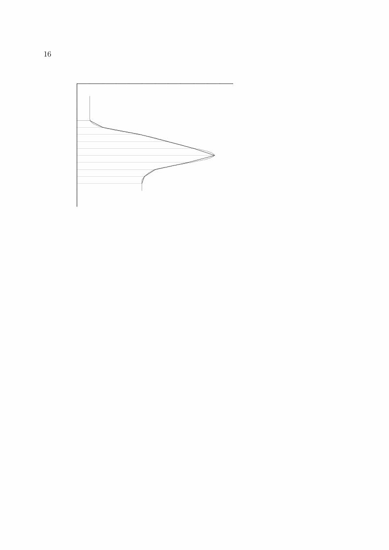
proved by using layers with linearly varying dielectric functions ε as depicted in fig.6
instead of those with constant ε.
16
zN+1
z2
z1
ε
z
Figure 6: Approximation of the real dielectric function by a system of layers with linearly varying
dielectric function ε
Using this ansatz the components of the individual layer matrices adopt the following
form:
m11s = 1 + (zn+1 − zn)2(
k2x2− ω2
c22εn+εn+1
6
)
m12s = zn+1 − zn
m21s = (zn+1 − zn)(
k2x − ω2
c2εn+εn+1
2
)
m22s = 1 + (zn+1 − zn)2(
k2x2− ω2
c2εn+2εn+1
6
)
m11p = 1 + (zn+1 − zn)2(
k2x2εn+εn+1
6εn− ω2
c2εn+2εn+1
6
)
m12p = (zn+1 − zn)εn+εn+1
2
m21p = (zn+1 − zn)(
k2x2( 1εn
+ 1εn+1
)− ω2
c2
)
m22p = 1 + (zn+1 − zn)2(
k2xεn+2εn+1
6εn+1− ω2
c22εn+εn+1
6
)
(52)
Setting εn = εn+1 within a layer in eqn. (52)yields the step profile approximation eqn. (51).
>From the equations for rp and rs, eqn. (49) and eqn. (48), the ellipsometric angles ∆ and
Ψ of arbitrary layer structures can be calculated using the basic equation of ellipsometry
eqn. 11.

17
6 Ellipsometry applied to ultrathin films
The previous section described an algorithm for the calculation on the reflectivity coeffi-
cients of given refractive index profiles. Profiles are only of importance if their characteris-
tic length scale is comparable to that of the probing beam. In many cases, i.e. adsorption
layer of nonionic surfactants at the air-water interface, there is a striking mismatch be-
tween interfacial height h and the wavelength of light λ. As a result certain peculiarities
exist which are discussed in this section [8].
The most striking limitation is a reduction of the measurable quantities. The presence
of an organic monolayer (refractive index 1.3-1.6) with a thickness below 2.5 nm does
not change the reflectivity |ri|2 and as a consequence there are no detectable changes in
Ψ . In the thin film limith ¼ λ the data analysis relies only on a single parameter,
namely changes in the phase ∆. Unfortunately the number of independent data cannot
be increased. Neither spectroscopic ellipsometry nor a variation of the angle of incidence
yield new independent data, instead all quantities remain strongly coupled. A sound
treatment is given in [9]. However, the sensitivity of an ellipsometric measurement can
be significantly increased by the choice of the angle of incidence. A sensitivity analysis is
given in [10].
The exact formula relating the reflectivity coefficients of a single homogeneous layer with
refractive index n1 =√ε1 in between two infinite media (n0 =
√ε0 and n2 =
√ε2) at an
angle of incidence ϕ is given by :
∆ = arctanIm
(
rprs
)
Re(
rprs
) withrp = |rp| · eiδr,p = r0,1,p+r1,2,pe−i2β
1+r0,1,pr1,2,pe−i2β
rs = |rs| · eiδr,s = r0,1,s+r1,2,se−i2β
1+r0,1,sr1,2,se−i2β
(53)
where the reflectivity coefficients r0,1,p, r1,2,p, r0,1,s and r1,2,s describing the reflection at
refractive index jumps n0 → n1 and n1 → n2 for Ýp- and Ýs-light are given by Fresnel’s laws.
β = 2π hλ
√
n21 − n2
0 sin2 ϕ accounts for the phase shift occuring in a single pass within the
adsorption layer.
If the layer thickness h is much smaller than the wavelength λ of light it is justified to
expand the complex reflectivity coefficients in a power series in terms of h/λ. The first

18
term in this expansion describes reflection at a monolayer.
∆ ≈4√ε0ε2π cosϕ sin2 ϕ
(ε0 − ε2)((ε0 + ε2) cos2 ϕ− ε0)· (ε1 − ε0)(ε2 − ε1)
ε1· hλ
(54)
If the refractive index is varying over the height of the layer, the term
(ε1 − ε0)(ε2 − ε1)
ε1· h
within eqn. (63) has to be replaced by an integral η across the interface:
η =
∫
(ε− ε0) (ε2 − ε)
εdz (55)
An ellipsometric experiment on a monolayer yields a quantity proportional to η. A sim-
plification of eqn. (55) reveals its physical meaning. Quite often, as for example in case
of adsorption of organic compounds onto solid supports [7], ε2 exceeds ε of the monolayer
while ε ≈ ε0.
Under these circumstances eqn. (55) can be further simplified:
η =ε2 − ε0
ε0
∫
(ε− ε0) dz (56)
A linear relationship between ε and the prevailing concentration c of amphiphile within
the adsorption layer is well established [11]
ε = ε0 + cdε
dc(57)
This relation yields a direct proportionality between the quantity η and the adsorbed
amount Γ.
η =ε2 − ε0
ε0
dε
dc
∫
c dz =ε2 − ε0
ε0
dε
dcΓ (58)
None of the assumptions which lead to eqn. (58) apply for adsorption layers at the liquid-
air interface and hence eqn. (55) cannot be further simplified. The relationship between
monolayer data and recorded changes remains obscure with no further simplifications
possible on the basis of Maxwell’s equations. A proportionality between ∆ and Γ may
hold but it cannot be established within this theoretical framework.

19
7 Microscopic model for reflection
Quantities such as refractive index or thickness are macroscopic quantities. Their meaning
at sub-monolayer coverage is not an obvious one. To bridge these inherent difficulties
several approaches have been developed aiming for a calculation of the optical properties
of a monolayer based on microscopic quantitities [12]. We follow here mainly a model
originally derived by Dignam et.al. [13, 14]. Explicit formulas are derived relating the
changes in ∆ to the polarizibility tensor of the adsorbed molecule and their number density
at the interface.
The adsorption layer is treated as a two dimensional sheet of dipoles driven by the external
laser field. The oscillating dipoles act as sources of radiation and the summation of all
their contributions yields the reflected beam in the far field.
The adsorption layer is considered as homogeneous, fluctuations in the orientation or
density occur on a length scale much smaller than the wavelength of light. These conditions
are usually fulfilled for adsorption layers of soluble surfactants.
The decisive new quantitity introduced by Dignam et. al. is the surface susceptibility
tensor ~γ
~γE0 = 4πPt (59)
which links the external electric field E0 to the resulting polarization per volume P, t
represents the thickness of the adsorbed layer. The polarization is given by the vector
sum of all dipole moments µj over all molecules j:
~γE0 = 4π∑
j
µj (60)
The local field at each dipole has two origins, the external laser field E0 and the dipolar
contribution which is proportional to E0.
EL = E0 + ~βE0 (61)
Each adsorbed molecule is characterized by its own tensor β. The induced dipole moment
of a molecule with a polarizability αj is given by
µj = ~αjEjL = ~αj(1 + ~βj)E0 (62)

20
with this notation the susceptibilty tensor ~γ reads:
~γ = 4π∑
j
~αj(1 + ~βj) (63)
In order to calculate β it is desirable to introduce the field Eij, which accounts for the
electric field at the position ri generated by the dipole of molecule j.
Eij = ~fijµj (64)
~fij = (3~ρij − 1)/r3ij for i 6= j (65)
~fij = 0 for i = j (66)
The projection operator ~ρ projects the induced dipole moment on the connection of the
molecules at site i and j.
Eij = ~fij~αij(1 + ~βj)E0 (67)
With the relation:
∑
j
Eij = ~βiEo (68)
~βi is given by
~βi =∑
j
~fij~αij
(
1 + ~βj
)
(69)
Each molecule is characterized by a tensor βj. For a further calculation certain assumptions
about the molecular distribution must be introduced. For adsorption layers of soluble
surfactants at the air-water interface it is a good approximation to consider β for all
molecules equal. The underlying molecular pircture is is that the adsorption layer consists
of one species of amphiphiles with a narrow angular distribution.

21
Under these conditions:
β =∑
j
~fij~αj (1 + β) (70)
meaning that
1 + β =
(
1−∑
j
~fij~α
)−1
(71)
With equation 63 the surface susceptibility tensor reads:
~γ =4πN~α
(1−∑
j~fij)~α
(72)
The number of molecules per unit area is denoted by N . For an uniaxial film with its
optical axis parallel to the surface normal the tangential t and normal n component of the
susceptibility tensor read:
γt =4πNαt
(1− 4π/3(N/te)αt
(73)
γn =4πNαn
(1− 8π/3(N/te)αn
(74)
The quantity te can be regarded as an effective thickness as defined as
te =8/3πN
∑
i6=j 1/r3ij
(75)
If the adsorption layer can be mathematically represented as adsorbed molecules on a
rectangular grid with an average next neighbour distance of a
te =8/3πa3N
(i2 + j2)−3/2= 0.935a3N (76)
At monolayer coverage N = 1/a2 the effective thickness is te = 0.935a. The adsorption
of molecules at the interface changes the optical properties of the system. The changes in
the ellipsometric angles are given by

22
ln
(
tanψ
tanψ0
)
+ i (∆−∆0) = δL (77)
In the thin film limit only changes in ∆ occur:
δLv =i4π
λcosϕ
δγt1− ε2
(
1 + δv, p1− εsδγn/δγtcot2 ϕ− 1/ε2
)
(78)
δγn,t denotes the difference of the susceptibility tensor between the film covered and the
bare surface, i =√−1, ϕ is the angle of incidence and λ is the wavelength of light.
Changes in the ellipsometric angle ∆ are given by the difference in L parallel and perpen-
dicular to the plane of incidence.
δ∆ = −i(δLp − δLs) (79)
The parallel component reads
−iδLp =4π
λcosϕ
δγt1− ε2
(
1 +1− ε2δγn/δγtcot2 ϕ− 1/ε2
)
(80)
whereas the perpendicular component is given by
−iδLs =4π
λcosϕ
δγt1− ε2
(81)
This model reflects the optical response at the molecular level, but the model suffers from
its complexity and high number of parameters, the values of which can only be assumed.
Since the macroscopic ansatz resulting in eqn. (54) comes to similar results with a properly
chosen dependence of the refractive index of the layer on the adsorbed amount, the use of
the microscopic model is not common in practical applications. In the following section
we will discuss some representative examples.
23
8 Adsorption layers of soluble surfactants
8.1 Importance of purification
Due to the peculiarities of surfactant synthesis, many surfactants contain trace impuri-
ties of higher surface activity than the main component. These trace impurities do not
influence most bulk properties. However, at the surface they are enriched and impurities
may even dominate the properties of the interface. This behaviour was first recognized
by Mysels [15] and a purification scheme using foam fractionation was proposed [16]. A
detailed discussion on artifacts caused by impurities can be found in [17].
In studies performed in our lab, we use a fully automated purification device developed by
Lunkenheimer et. al. which ensures a complete removal of these unwanted trace impurities
[18]. The aqueous stock solution undergoes numerous of purification cycles consisting of
a) compression of the surface layer, b) its removal with the aid of a capillary, c) dilation to
an increased surface and d) formation of a new adsorption layer. At the end of each cycle
the surface tension σe is measured. The solution is referred to as surface chemically pure
grade if σe remains constant in between subsequent cycles. Quite frequently more than
300 cycles and a total time of several days are required to achieve the desired state. The
sample preparation is time consuming and tedious but mandatory for the investigation of
equilibrium properties of adsorption layers of soluble surfactants at the air-liquid interface.
8.2 Physicochemical properties of our model systems
In the following we discuss the interfacial properties of two related amphiphiles, the
cationic amphiphile 1-dodecyl-4-dimethylaminopyridinium bromide, C12-DMP, and the
closely related nonionic 2-(4’dimethylaminopyridinio)-dodecanoate, C12-DMP betaine.
The corresponding chemical structures are depicted in fig. 7 together with their equi-
librium surface tension isotherms. The synthesis is described in [19].
Both components are classical amphiphiles and resemble all common features such as the
existence of a critical micelle concentration cmc. The members of the homologous series
of the alkyl-dimethylaminopyridinium bromide are strong electrolytes and follow the pre-

24
dictions of Debye-Huckel theory as experimentally verified by conductivity measurements.
For solubility reasons we used 1-butyl-4-dimethylaminopyridinium bromide instead of the
C12 representative of the homologous series which gave us experimental access to a wider
concentration range. Debye-Huckel predicts a proportionality of the activity coefficient
to the square root of the ionic strength for aqueous solutions of 1:1 electrolytes which is
indeed observed in our experiment.
N N
O O
Br
N N
1E-6 1E-5 1E-4 1E-3 0.0135
40
45
50
55
60
65
70
75
surf
ace
tens
ion
[mN
/m]
concentration
on
[mol/l]
Figure 7: Chemical structures of the cationic amphiphile 1-dodecyl-4-dimethylaminopyridinium bro-
mide, C12-DMP bromide, and the closely related nonionic 2-(4’dimethylaminopyridinio)-dodecanoate,
C12-DMP betaine. The equilibrium surface tension σe of a purified aqueous solution of the ionic C12-DMP
bromide(squares) and the nonionic C12-DMP betaine(triangles) as a function of the bulk concentration
co. (redrawn from [20])
8.3 Adsorption layer of a nonionic surfactant
The ellipsometric isotherm ∆−∆0 of the nonionic amhiphile C12-DMP betaine is shown
in Fig. 8. It decreases in a monotoneous fashion and reaches a limiting value at higher
concentration. In order to assess its physical meaning we compare ∆−∆0 to the surface
excess retrieved from the surface tension isotherm Fig. 7. According to Gibbs’ fundamental
law:
Γ = − 1
mRT· dσe
d ln a≈ − 1
mRT· dσe
d ln c(82)
the total surface excess Γ is given by the derivative of the surface tension isotherm σe(c).

25
Γ is then compared to the changes of the ellipsometric quantity ∆−∆0. The inset of Fig. 8
presents the result. The surface excess as given by the slope of the surface tension isotherm
is compared to the ellipsometric response at each concentration. Obviously the relation
between both quantities can be described by a straight line. Hence, experimental evidence
has been provided that ellipsometry measures indeed the surface excess of the adsorption
layer of the soluble nonionic amphiphile. Since optics measures refractive indices which
are not very sensitive to molecular details we anticipate that this holds for a wider class
of materials.
0.0 0.5 1.0 1.5 2.0 2.5 3.0-2.5
-2.0
-1.5
-1.0
-0.5
0.0
0 1 2 3 4 5 6 7 8-2.5
-2.0
-1.5
-1.0
-0.5
0.0
d ∆ [
°]
c0 [mmol/l]
d ∆
[°]
- δσ / δ ln(c0)
Figure 8: Ellipsometric isotherm of the nonionic C12-DMP betain. The ellipsometric isotherm decreases
in a monotonic fashion and is proportional to the surface excess as can be seen in the inset, which compares
the surface excess according to Gibbs and the ellipsometric response. (redrawn from [20])
8.4 Ionic surfactant at the air-water interface
In the previous section it was shown that in spite of the uncertainties from the mathemat-
ical point of view concerning the interpretation of eqn. (55) a proportionality between ∆
and Γ can be established by a comparison of thermodynamic and ellipsometric data for a
nonionic surfactant at the air-water interface. In the following we will discuss a measure-

26
ment carried out on adsorption layers of an ionic surfactant. It will be demonstrated that
there are major differences between the two model systems.
0.0 0.5 1.0 1.5 2.0 2.5 3.0 3.5
-3.5
-3.0
-2.5
-2.0
-1.5
-1.0
-0.5
0.0
N [1
/nm
2 ]
d ∆ [
°]
c0 [mmol/l]
0123
0.0 0.5 1.0 1.5 2.0 2.5-3.0
-2.5
-2.0
-1.5
-1.0
-0.5
0.0
d ∆ [
°]
N [1/nm2 ]
Figure 9: Characterization of the equilibrium properties of the adsorption layer by ellipsometry and Sur-
face second harmonic generation, SHG. The SHG-signal√
I2ω(P = 45, A = 90) (circles) is proportional to
the surface coverage and increases monotonously with the bulk concentration. The ellipsometric quantity
d∆ = ∆ −∆0 (triangles) shows an extremum at an intermediate concentration far below the cmc. The
inset clearly shows the nonmonotonic dependency of d∆ on the adsorbed amount. (redrawn from [20])
Fig. 9 shows the ellipsometric isotherm ∆−∆0(triangles) of the cationic surfactant C12-
DMP bromide. A pronounced non-monotonic behaviour is shown with an extremum at
an intermidiate concentration far below the cmc. Also shown is the number density of
amphiphiles adsorbed to the interface (circles) as determined by Surface second harmonic
generation (SHG). At these bulk concentrations the measured number density equals the
surface excess Γ. SHG reveals a monotoneous increase in the surface excess in qualitative
agreement to a thermodynamic analysis within the Gibb’s framework. The data also
clearly prove that the ellipsometric quantity need not be proportional to the adsorbed
amount for a soluble ionic surfactant. What causes the nonmonotonous behaviour and
how can it be understood?
In the following we discuss some possible scenarios:

27
Scenario 1: Filling up the adsorption layer
The adsorption layer is described as an isotropic optical layer of constant thickness with a
refractive index nlayer which depends on the surface coverage [21]. Within this model there
are two distinct surface concentrations which lead to a vanishing d∆ = ∆−∆0 = 0. At
very low coverage the refractive index of the layer matches the one of air nlayer = nair = 1
and at an intermediate surface coverage the surface layer adopts the very same refractive
index as the water bulk phase nlayer = nwater = 1.332. Consequently there has to be
an extremum in between. The resulting d∆(nlayer)-curve is depicted in Fig. 10. The
geometrical dimension of the molecules has been used as thickness of the layer.
1.0 1.1 1.2 1.3 1.4 1.5-3.5
-3.0
-2.5
-2.0
-1.5
-1.0
-0.5
0.0
0.5
1.0
1.5
d ∆ [
°]
nlayer
Figure 10: Simulation of the effect of a changing refractive index of a layer of constant thickness
h = 2.1nm on the ellipsometric signal d∆.
Obviously this scenario is not suitable to explain the measurement, the model predicts
even a wrong sign of d∆max ≈ 1.75 ! The experimental data require that nlayer > nwater
at all concentration. This means, water instead of air is the effective environment of this
particular amphiphile within the adsorption layer.

28
Scenario 2: Effect of anisotropy
The following provides an estimation if changes in the molecular orientation may be respon-
sible for the surprising features in the ellipsometric isotherm. The following assumptions
were made in order to estimate an upper limit for this effect:
• The optical model is that of an uniaxial layer with the optical axis normal to the
interface. The molecular arrangement is C∞V which has been experimentally verified
for the headgroups by polarization dependent SHG measurements.
• The thickness of the adsorbed layer and the mean tilt angle of the molecules within
the layer change with their number density N at the interface. Within the investi-
gated number density range the thickness increases from 1nm to 1.9nm proportional
to the cosine of the tilt angle which is assumed to change from around 70 to 40.
• The whole molecule, including the head group, is assumed to change its tilt angle.
The molecules are assumed to be all-trans and perfectly aligned which would yield
the maximum possible change in anisotropy.
• The refractive index for an E-vector along the length axis of the molecule is naxis =
1.56, while the refractive index for an E-vector perpendicular to the long axis of
the molecule is nperp = 1.48. Both refractive indices have been taken from Riegler
et.al. [22] and rely on a combination of X-ray reflection data with ellipsometric
measurements of monolayers of behenic acid at the air-water interface for a densely
packed and perfectly oriented apmphiphiles. In our case the actual refractive indices
will depend on the prevailing volume concentration and the data are therefore an
upper limit.
The calculated d∆(N) versus density-curve is plotted in Fig. 11. Obviously a change of
the molecular tilt leads to changes in d∆, but cannot account for the measured pronounced
extremum. In addition it is impossible to reach d∆ = −2.77, which is the minimum of
the measured curve, with reasonable parameters for the anisotropic layer. An increase
in anisotropy has the same impact on the ellipsometric measurements as a reduction of

29
0.0 0.5 1.0 1.5 2.0 2.5-1.6
-1.4
-1.2
-1.0
-0.8
-0.6
-0.4
-0.2
0.0
d ∆ [°
]
N [1/nm2 ]
Figure 11: Investigation of the impact of anisotropy on the ellipsometric signal. The ellipsometric signal
d∆ calculated in dependence of the number density of adsorbed molecules N. A molecular length of 2.1
nm and a refractive index of naxis = 1.56 for an E-vector along and of nperp = 1.48 for an E-vector
perpendicular to the molecular axis were used. The layer thickness (1.0nm to 1.9nm), the tilt angle (70
down to 40), ns and np were all assumed to be dependent on the surface coverage.
the layer thickness; hence, the only way to get nearer to d∆ = −2.77 is to diminish the
anisotropy!
At this point we would like to point out that the assumptions made for this simulation
are highly exaggerating the effect of the anisotropy. The SHG measurements reveal that
the heads do not change their tilt angle at all. In other words that only the tails may
change their tilt, which results in an even thinner anisotropic layer and therefore a smaller
effect. Additionally the tails are certainly neither all-trans nor perfectly oriented even at
the highest coverage measured 0.37nm2/molecule. For these reasons Fig. 11 represents an
upper limit of the impact of anisotropy. The real effect is by far smaller for the surface
coverages encountered here, which means that anisotropy cannot account for the surprising
feature of the ellipsometric isotherm.

30
Scenario 3: Changing the counterion distribution
Ellipsometry probes the complete interfacial architecture. The reflected light is generated
within the transition region between the two adjacent bulk phases, air and aqueous surfac-
tant solution. The electric double layer has to be explicetely considered. Hence, changes
in the ion distribution at higher concentrations may cause the observed feature in the
ellipsometric isotherm.
The classical model of a charged double layer has been developed by Gouy, Chapman and
Stern. The interface is described by two distinct regions: a compact layer consisting of
the positively charged adsorbed amphiphiles with some directly adsorbed counterions and
a diffuse layer of counterions.
The ion distribution within the diffuse layer is given by the solution of the Poisson equation
which relates the divergence of the gradient of the electric potential Φ to the charge density
ρ at that point (see for instance [23, 24]):
div gradΦ =4Φ =− ρ
εoεr(83)
The compact layer is positively charged and in contact with an electrolyte solution which
forms a diffuse layer of charges. The ion concentration distribution within the electrical
potential Φ obeys Boltzmann:
c− = c−o ez−eΦkBT c+ = c+o e
− z+eΦkBT (84)
where z− and z+ are the valencies of the anions and cations respectively. For a symmetric
electrolyte solution (−z− = z+ = z and c−o = c+o = co) eqn.(84) leads to a net charge of
the ion cloud of
ρ = ze(c+ − c−) = −2coze sinhzeΦ
kBT(85)
The combination of eqn.(85) with the Poisson eqn.(83) yields a differential equation in the
electric potential Φ . In our case the potential is only a function of the normal coordinate
to the surface x. It is convenient to define a reduced potential

31
y =zeΦ
kBTyo =
zeΦo
kBT(86)
which further simplifies the equations and results in
d2y
dx2=
2coz2e2
kBTεoεrsinh y = κ2 sinh y (87)
The integration of equation (87) with the boundary conditions (y = 0 and dy/dx = 0) for
x = ∞ and y = yo at x = 0 lead to the Gouy-Chapmann solution of the reduced potential
within the diffuse layer:
ey/2 =eyo/2 + 1 +
(
eyo/2 − 1)
e−κx
eyo/2 + 1− (eyo/2 − 1) e−κx(88)
Hence, knowing the charge of the compact layer the ion distribution can be modelled. The
crux of Stern’s treatment is the estimation to which extent ions enter the compact layer
and reduce the surface potential. The ion distribution between compact and diffuse layer
cannot be easily experimentally established, for example surface potential measurements
cannot measure this distribution.
The optical analysis requires the translation of the prevailing distribution of molecules
and ions within the interphase into a corresponding refractive index profile. The reflec-
tivity coefficients can then be calculated on the basis the previously discussed numerical
algorithms for stratified media. Two elements dominate the refractive index profile and
hence the reflectivity properties, the topmost monolayer of the amphiphile and the distri-
bution of ions within the diffuse layer. The excess of ions within the diffuse layer leads
to a slightly elevated refractive index as compared to the bulk of the aqueous surfactant
solution. The typical dimensions of the diffuse layer are on the order of 10 nm and this
fairly wide extension leads to a profound impact on ∆, since the topmost monolayer has
a normal extension of only 2 nm. The solution of the potential Φ plugged into equation
(85) yields the distribution of anions and cations within the diffuse layer. The prevailing
charge distribution is determined by the surface charge of the topmost monolayer. The
refractive index profile is then determined by the ion distribution by a multiplication with

32
the refractive index increment dn/dc which has been independently measured with an
Abbe refractometer.
x x
xx
c
c
n
n
high bulk concentration
low bulk concentration
1.332
1.332
0
00
0
0
0
2
2 2
2
a
b
Figure 12: The interphase of a soluble cationic surfactant at the air-water interface at low (a) and high
(b) bulk concentration. It consists of a charged topmost cationic monolayer, a diffuse layer of counterions
and at higher concentrations a compact layer of directly adsorbed counterions. The charge density of the
topmost monolayer reduced by the charge of the inner Stern layer determines the ion distribution within
the diffuse layer. The prevailing ion distribution is given by solution of the nonlinear Poisson-Boltzmann
equation. The excess of ions can be readily translated in a corresponding refractive index profile. The
profile determines the reflectivity properties. Ellipsometric data modeled within this framework allow an
estimation of the extent to which ions enter the compact layer.
Fig. 12 sketches the model for the interface. At lower surface coverage most of the ions are
spread out within the diffuse layer leading to a pronounced refractive index profile. The
situation is sketched in Fig. 12a. At higher concentration some ions enter the adsorption
layer and form ion pairs with the headgroups accounted with a lower dn/dc-value as
compared to the bulk phase. The formation of this Stern layer effectively reduces the
surface charge and as a consequence the extension and the magnitude of the refractive
index profile of the diffuse layer decrease. This situation is sketched in Fig. 12b.
This model has been used for monitoring the formation of the Stern layer. The ion
distribution within the diffuse layer is determined by the total effective charge density
at the interface. The SHG measurements yield the number density and charge density

33
2.2 2.4 2.6 2.8 3.0 3.2 3.4 3.6
0.4
0.8
1.2
1.6
2.0
c0 [ mmol / l ]
s [e
/nm
2 ]
Figure 13: The charge density of the compact Stern layer has been retrieved by optical means. The
surface charge refers to the number density of the cationic amphiphile reduced by the number of directly
bound ions within the Stern layer.
produced by the cationic amphiphilic monolayer. The effective charge density at the
interface is given by this value reduced by the number density of counterions within the
Stern layer. The corresponding refractive index of Stern and topmost monolayer is given
by an effective medium approach. Hence the optical properties of the monolayer are known
by independent means. Furthermore the refractive index profile of the diffuse layer is given
once the effective charge density at the interface is known. We used the experimental data
in order to retrieve the corresponding effective surface charge density. The results are
depicted in Fig. 13 starting in the vicinity of the extremum of the ellipsometric isotherm.
Hence, with this model we are able to monitor by purely optical means the extent to which
ions enter the compact Stern layer.
In short, ellipsometry applied to adsorption layers of ionic soluble surfactants does not
measure the surface excess. The ellipsometric signal may show a non-monotonic behaviour
which is caused by a redistribution of the ions between compact and diffuse layer. The
data analysis within the classical model of a charged double layer yields an estimate of
the prevailing ion distribution.
Ellipsometry applied to adsorption layers of nonionic surfactant directly yields the surface

34
excess. It is therefore a valuable alternative to surface tension measurements, especially if
one considers rheological properties which require higher derivatives of the surface tension
isotherm.
8.5 Kinetics of absorption
Rapidly expanding liquid surfaces occur in many technical processes such as foam forma-
tion, spraying or painting, they are also omnipresent in nature, i.e. the oxygen exchange
in the lung. Surfactants play a crucial role in these processes. They stabilize the new
surfaces by a reduction of the surface tension. Inhomogeneities in surface coverage lead
to gradients in surface tension which in turn have a strong impact on bulk hydrodynamic
flow, a phenomenon also known as Marangoni flow. The overall dynamic behaviour is
very complex and despite many efforts far from understood [25]. The investigation re-
quires time resolution within the ms regime putting severe limitations on the choice of
the experimental technique. The maximum bubble pressure method [25] is most often
used to perform these types of studies but ellipsometry offers an interesting alternative
to supplement these investigations. This method relies on surface tension measurements
and the surface coverage is obtained using the equilibrium surface isotherm. The under-
lying assumption is that the surface is locally at equilibrium, however, in the time regime
of interest this may not be the case. As outlined in the theoretical section ellipsometry
measures directly the surface coverage for nonionic surfactants and provides in addition
the requested time resolution. The challenging part is the design of an experiment with
precisely defined boundary conditions required for modeling the underlying physics lead-
ing to the observed kinetic behavior. The most promising approaches produce an interface
with a non-equilibrium surface coverage, and maintain that surface coverage through the
flow of fluid in and out of the control volume. To satisfy the requirement of well-defined
boundary conditions, at the beginning of the flow a freshly formed surface must be created.
Several arrangements have been suggested such as the inclined plate [25], the overflowing
cylinder [26] or the use of a jet [27]. In all these approaches the surface has a defined age
at a given spot, hence the desired dynamic picture of the surfactant adsorption is obtained
by moving the sample relative to the light beam.

35
JA
A
PMT L
PQ
BMF
SS
Figure 14: Setup for an ellipsometric measurement on a jet. The distance between laser spot and nozzle
determines the age of the surface. (redrawn from Langmuir 15, 7530-7533 (1999))
The overflowing cylinder with its flat surface is very well suited for optical reflection tech-
nique. Water is pumped vertically trough a cylinder and allowed to flow over the rim in
a radial flow pattern. This experiment covers the time regime of 0.1 − 1s and has been
successfully used by Penfold et.al. [28] in neutron reflectometry and ellipsometric experi-
ments. A precision in the determination of the dynamic surface excess of 2 · 10−8mol/m2
has been demonstrated. Neutron reflectivity enabled the calibration of the ellipsometric
data which is important to avoid artifacts caused by changes in the ion distribution of ionic
surfactants. The more interesting time range of 1 − 20ms is covered by jet techniques.
The surfactant solution is pumped with a high speed through a nozzle. An ellipsometric
experiment performed on a jet is quite demanding and many subtle problems are caused
by the curved surface acting as a cylindrical lens. A recent feasibility study of Hutchi-
son et.al. demonstrates that these problems can be overcome [29]. The adsorption of a
cationic surfactant was monitored and the time dependence was found to obeye the Ward-
Tordai equation [30] providing evidence for a diffusion controlled adsorption kinetics of
the surfactant in this time regime. These studies suffer from a simultaneous measurement
of the flow field which is required to assess Maragoni currents induced by surface tension
gradients.

36
0.00 0.04 0.08 0.12 0.160.0
0.5
1.0
1.5
2.0
2.5
Time1/2 / s1/2
Γ Dyn
amic /
10-6 m
ol m
-2
Figure 15: Surface coverage measured with the setup sketched in Fig. 14. (redrawn from Langmuir 15,
7530-7533 (1999))
9 Principle of imaging ellipsometry
Some surfaces under investigation are laterally inhomogeneous on a micrometer scale due
to variations in the thickness or surface composition or due to changes in the orientational
order of the molecules at the interface. In this case the lateral inhomogeneity is imparted
to the properties of the reflected light. The most well-known imaging technique for a
visualization of these features is Brewster Angle Microscopy BAM [31, 34] which has
been successfully employed for characterizing the phase diagrams and the morphology of
Langmuir films. BAM is based on the principle that the reflectivity of the Ýp-polarized light
is zero at the Brewster angle. Any modification of the Brewster conditions, as for instance
the presence of a single monolayer, modifies the reflectivity. A decisive advantage of this
method vs. fluorescence microscopy [35] is that fluorescent labelling is not required. Also
the internal structures of domains can be assessed.
Ellipsometry can also be extended to an imaging technique which offers a wider field of
applications [9]. In contrast to BAM, imaging is not bound to the existence of a Brewster
angle and can even be employed for the investigation of monolayers on highly reflecting
supports.
Fig. (16a) provides a Nullellipsometric image of a self assembled monolayer of (Dimethyl-

37
Figure 16: The lateral inhomogeneitity is transformed in the state of polarization. a) Nullellipsometric
image of a self assembled monolayer on a silicon wafer. The monolayer was patterned with the aid of a
mask and UV-light. The difference in the thickness between the dark and bright regions is 0.8nm b) At
high magnification problems arise due to the limited depth of field. The width of the bars are 1.9µm, the
mesh size is 10µm and imaging is performed at an angle of 53
chlorosilyl)-2-(p,m-chloromethylphenyl)ethan on silicon. The monolayer was photochem-
ically pattererned using UV-irradiation and an electron microscopy grid as a mask. The
difference in the thickness between dark and bright regions is 0.8 nm demonstrating the
high vertical resolution of this technique. At a higher magnification there are certain
problems arising from the limitation of the depth-of-field.
9.1 Depth of field problem
All the above mentioned imaging techniques work under an oblique angle of incidence and
as a result some peculiarities exist. Imaging under an oblique angle of incidence imposes
certain restrictions on the diameter and working distance of the objective. As a result the
resolution is limited to about 1− 3µm. A discussion of this issue can be found in [32].
The depth of field, t, of an objective is given by the numerical aperture A, the refractive
index n of the ambient medium, and the wavelength λ according to [33]:
t =nλ
A2(89)

38
Depending on the angle of incidence, ϕ, and the numerical aperture, A, only a region of
the illuminated part of the sample is in focus. This region is of the order of 1 − 50µm.
This problem is illustrated in Figure (16b). The size of a bar is 1.9µm, the mesh size is
10µm and imaging was performed at ϕ = 53.
The depth-of-field problem is a severe limitation at higher magnification. A straightfor-
ward solution consists of a scan of the objective [34]. Only the area in focus is recorded
and the complete image is constructed by many stripes by imaging processing software.
This procedure yields sharp images of static objects. At the oil-water or air-water interface
it is only of limited use due to the prevailing convection.
Figure 17: Principle of ellipsometric microscopy. Full arrows symbolise the light path of illumination,
broken arrows stand for the observation, respectively. A parallel beam of polarised light is focussed into
an off-axis spot in the back focal plane of the lens. In the front focal plane of the lens, where the object
is located, this results in a parallel polarised beam of light hitting the object under a shallow angle of
incidence. Light reflected by the object is collected by the lens, passes a motorised polarization analyzer
and is focused onto a digital CCD camera. For clarity, several optical elements are omitted. (redrawn
from [36])
An elegant approach which overcomes these difficulties was suggested in the group of
Sackmann et al.. A parallel polarized laser beam was focused to an off axis spot in the
back focal plane of a microscope objective of high numerical aperture. The sample which is
located in the front plane is then illuminated by a parallel polarized beam of light incident
on the sample under an oblique angle. The exact angle of incidence is controlled by the
39
exact position of the laser focus in the back focal plane. The image is formed by the same
objective used for illumination and the complete image is in focus [36].
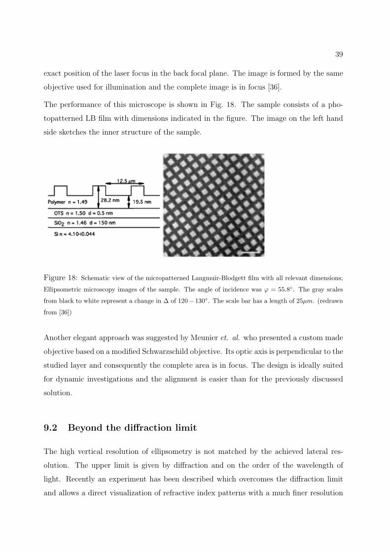
The performance of this microscope is shown in Fig. 18. The sample consists of a pho-
topatterned LB film with dimensions indicated in the figure. The image on the left hand
side sketches the inner structure of the sample.
Figure 18: Schematic view of the micropatterned Langmuir-Blodgett film with all relevant dimensions;
Ellipsometric microscopy images of the sample. The angle of incidence was ϕ = 55.8. The gray scales
from black to white represent a change in ∆ of 120− 130. The scale bar has a length of 25µm. (redrawn
from [36])
Another elegant approach was suggested by Meunier et. al. who presented a custom made
objective based on a modified Schwarzschild objective. Its optic axis is perpendicular to the
studied layer and consequently the complete area is in focus. The design is ideally suited
for dynamic investigations and the alignment is easier than for the previously discussed
solution.
9.2 Beyond the diffraction limit
The high vertical resolution of ellipsometry is not matched by the achieved lateral res-
olution. The upper limit is given by diffraction and on the order of the wavelength of
light. Recently an experiment has been described which overcomes the diffraction limit
and allows a direct visualization of refractive index patterns with a much finer resolution

40
[37]. The arrangement is based on a combination of Atomic Force Microscopy (AFM) and
Ellipsometry and the AFM tip dimensions determines the resolution.
The sample of interest is mounted on the base of a prism. The ellipsometer is operated
in the null mode and the total reflected light at the prism base is completely cancelled by
the setting of the polarization optics. This null setting is kept constant during the course
of the experiment. The metal AFM tip couples to the evanescent field and depending on
the local optical properties of the sample the null setting is out of tune. The intensity
at the detector is monitored while carrying out a topographic scan with a conventional
Atomic Force Microscope. Thus two images are simultaneously generated: a topographic
image by the AFM tip and an ellipsometric image which relates the intensity reading at
the detector with the x,y position of the tip. The latter contains information on refractive
index inhomogenity. This technique allowed for instance a visualization of 10 nm CDTe
particles within a polymer matrix. The topographic scan was not able to identify the
particles within the spincoated polymer film. However, due to the differences in the
refractive index it could be visualized by the ellipsometric image.
Compensator
Polarizer
Analyzer
Detector
Laser beam
AFM tip
Prism with sample
Figure 19: Sketch of the used apparatus

41
References
[1] M. Born, Optik, Springer Verlag, New York, Heidelberg (1998)
[2] D. S. Kliger, J. W. Lewis, C. Randall, Polarized Light in optics and spectroscopy,
Academic Press, Harcout Brace Javanovich Publishers, Boston (1990)
[3] R. M. Azzam, N.M. Bashara, Ellipsometry and Polarized Light,
North Holland Publication, Amsterdam (1979)
[4] R.C. Jones, J. Opt. Soc. Am 16, 488 (1941)
[5] S.N. Jasperson, S.E. Schnatterly, Rev. Sci. Instr. 40 , 761 (1969)
[6] J. Lekner, Theory of Reflection, Martinus Nijhoff Publishers, Boston, (1987)
[7] T. Kull, T. Nylander, F. Tiberg, N. Wahlgren, Langmuir 13, 5141 (1997)
[8] R. Teppner, S. Bae, K. Haage, H. Motschmann, Langmuir 15, 7002 (1999)
[9] R. Reiter, H. Motschmann, H. Orendi, A. Nemetz, W. Knoll, Langmuir 8, 1784 (1992)
[10] C. Flueraru, S. Schrader, V. Zauls, H. Motschmann, Thin Solid Films 379, 15 (2000)
[11] H. Motschmann, M. Stamm, C. Toprakcioglu, Macromolecules 24, 3681 (1991)
[12] J. Lekner, P.J. Castle, Physica 101A, 89 (1980)
[13] M.J. Dignam, M. Moskovits, J. Chem. Soc. Faraday II 69, 56 (1973)
[14] M.J. Dignam, J. Fedyk, J. Phys. (Paris) 38, C5-57 (1977).
[15] P.H. Elworthy, K.J. Mysels, J. Coll. Int. Sci. , 331 (1966)
[16] K.J. Mysels, A. Florence, J. Coll. Int. Sci. 43, 577 (1973)
[17] K. Lunkenheimer, J. Coll. Int. Sci. 131, 580 (1989)
[18] K. Lunkenheimer, H.J. Pergande, H. Kruger, Rev. Sci. Instr. 58, 2313 (1987)
[19] K. Haage, H. Motschmann, S. Bae, E. Grundemann, Colloids and Surfaces (in press)

42
[20] R. Teppner, K. Haage, D. Wantke , H. Motschmann,
J.Phys.Chem.B 104, 11489 (2000)
[21] T. Pfohl, H. Mohwald, H. Riegler, Langmuir 14, 5285 (1998)
[22] M. Paudler, J. Ruths, H. Riegler, Langmuir 8, 184 (1992)
[23] D.F. Evans, H. Wennerstrom, The Colloidal Domain,
VCH Publishers, New York (1994)
[24] A.W. Adamson, Physical Chemistry of Surfaces, Wiley & Sons, New York (1993)
[25] S.S. Dukhin, G. Kretzschmar, R. Miller,
Dynamics of Adsorption at Liquid Interfaces, Elsevier, Amsterdam (1995)
[26] D.J.M. Bergink-Martens, H.J. Bos, A. Prins, B.C. Schulte, J. Coll. Int. Sci. 138
(1990); D.J.M. Bergink-Martens, H.J. Bos, A. Prins, J. Coll. Int. Sci. 165, 221 (1994)
[27] B.A. Noskov, Adv. Colloid Interface Sci. 69, 63 (1996)
[28] S. Manning-Benson, S. R. W. Parker, C. D. Bain, J. Penfold, Langmuir 14, 990 (1998)
[29] J. Hutchison, D. Klenerman, S. Manning-Benson, C. Bain, Langmuir 15, 7530 (1999)
[30] A.F.H. Ward, L. Tordai, J. Chem. Phys. 14, 453 (1946)
[31] D. Honig, D. Mobius, J. Phys. Chem 95, 4590 (1991)
[32] M. Harke, R. Teppner, O. Schulz, H. Orendi, H. Motschmann,
Rev. Sci. Instrum. 68, 8, 3130 (1997)
[33] H. Riesenberg Handbook of Microscopy, VEB Verlag Technik, Berlin (1988)
[34] S. Henon, J. Meunier, Rev. Sci. Instr. 62, 936 (1991)
[35] M. Losche, E. Sackmann, H. Mohwald, Ber. Bunsenges. Phys. Chem. 10, 848 (1983)
[36] K.R. Neumaier, G. Elender, E. Sackmann, R. Merkel,
Europhysics Letters 49 (1), 14 (2000)
[37] P. Karageorgiev, H. Orendi, B. Stiller, L. Brehmer, Appl. Phys. Lett., (2001) in press
Top Related