


Languages
Pages
Legal


i Frontier Economics | April 2015 Confidential
© Frontier Economics Pty. Ltd., Australia.
Electricity market forecasts: 2015 A REPORT PREPARED FOR THE AUSTRALIAN ENERGY MARKET
OPERATOR (AEMO): FINAL
April 2015


i Frontier Economics | April 2015 Confidential
Contents 15-04-20 AEMO 2015 Electricity price forecasts -
Final External.docx
Electricity market forecasts: 2015
Executive summary v
1 Introduction 1
1.1 Outline 1
1.2 Structure of the report 2
2 AEMO energy market scenarios 3
2.1 Network costs 3
2.2 Demand 1
2.3 Carbon price 4
2.4 Scenarios and results (impact on prices) 5
3 Retail electricity forecasts to 2039/40 7
3.1 Overview 7
3.2 Historical prices 7
3.3 Summary results (residential, medium case) 8
3.4 Queensland 10
3.5 NSW and ACT 18
3.6 Victoria 26
3.7 South Australia 34
3.8 Tasmania 42
Appendix A Modelling methodologies 51

ii Frontier Economics | April 2015 Confidential
Tables and figures Final
Electricity market forecasts: 2015
Figures
Figure 1: Electricity: residential retail, all states, Real index, Medium vi
Figure 2 Overview of modelling approach 2
Figure 3 Assumed electricity demand: QLD 1
Figure 4 Assumed electricity demand: NSW 2
Figure 5 Assumed electricity demand: SA 2
Figure 6 Assumed electricity demand: VIC 3
Figure 7 Assumed electricity demand: TAS 3
Figure 8 Assumed carbon price by scenario 4
Figure 9 Electricity prices: stylised demand-side versus supply-side factors 6
Figure 10: Electricity: residential retail, all states, Real index, Medium case 9
Figure 11 Electricity: Historical residential retail, Qld, nominal c/kWh 10
Figure 12 Electricity: Historical business and residential retail, Qld, nominal
c/kWh 11
Figure 13 Electricity: residential retail by case, Qld (Real index) 13
Figure 14 Electricity: business retail by case, Qld (Real index) 13
Figure 15 Electricity: residential retail by component, Qld, Medium 14
Figure 16 Electricity: residential retail by component, Qld, Low demand 16
Figure 17 Electricity: residential retail by component, Qld, High demand 16
Figure 18 Electricity: residential retail, Qld, real index, compared with
previous projections 17
Figure 19 Electricity: Historical residential retail, NSW and ACT, nominal
c/kWh 18
Figure 20 Electricity: Historical business and residential retail, NSW and ACT,
nominal c/kWh 19
Figure 21 Electricity: residential retail by case, NSW (Real index) 21
Figure 22 Electricity: business retail by case, NSW (Real index) 21
Figure 23 Electricity: residential retail by component, NSW, Medium 22
Figure 24 Electricity: residential retail by component, NSW, Low demand 24
Figure 25 Electricity: residential retail by component, NSW, High demand 24

Confidential April 2015 | Frontier Economics iii
Final Tables and figures
Figure 26 Electricity: residential retail, NSW, real index, compared with
previous projections 25
Figure 27 Electricity: Historical residential retail, VIC, nominal c/kWh 26
Figure 28 Electricity: Historical business and residential retail, VIC, nominal
c/kWh 27
Figure 29 Electricity: residential retail by case, VIC (Real index) 29
Figure 30 Electricity: business retail by case, VIC (Real index) 29
Figure 31 Electricity: residential retail by component, VIC, Medium 30
Figure 32 Electricity: residential retail by component, VIC, Low demand 32
Figure 33 Electricity: residential retail by component, VIC, High demand 32
Figure 34 Electricity: residential retail, VIC, real index, compared with
previous projections 33
Figure 35 Electricity: Historical residential retail, SA, nominal c/kWh 34
Figure 36 Electricity: Historical business and residential retail, SA, nominal
c/kWh 35
Figure 37 Electricity: residential retail by case, SA (Real index) 37
Figure 38 Electricity: business retail by case, SA (Real index) 37
Figure 39 Electricity: residential retail by component, SA, Medium 38
Figure 40 Electricity: residential retail by component, SA, Low demand 40
Figure 41 Electricity: residential retail by component, SA, High demand 40
Figure 42 Electricity: residential retail, SA, real index, compared with previous
projections 41
Figure 43 Electricity: Historical residential retail, TAS, nominal c/kWh 42
Figure 44 Electricity: Historical business and residential retail, TAS, nominal
c/kWh 43
Figure 45 Electricity: residential retail by case, TAS (Real index) 45
Figure 46 Electricity: business retail by case, TAS (Real index) 45
Figure 47 Electricity: residential retail by component, TAS, Medium 46
Figure 48 Electricity: residential retail by component, TAS, Low demand 48
Figure 49 Electricity: residential retail by component, TAS, High demand 48
Figure 50 Electricity: residential retail, Tas, real index, compared with
previous projections 49

iv Frontier Economics | April 2015 Confidential
Tables and figures Final
Tables
Table 1:Summary of key assumptions by energy scenario 1
Table 2: Regulatory timetable 4
Table 3 Price change and contribution by component, Qld, real $ (Medium) 15
Table 4 Price change and contribution by component, NSW, real $ (Medium)
23
Table 5 Price change and contribution by component, Vic, real $ (Medium) 31
Table 6 Price change and contribution by component, SA, real $ (Medium) 39
Table 7 Price change and contribution by component, Tas, real $ (Medium) 47

Confidential April 2015 | Frontier Economics v
Final Executive summary
Executive summary
This report presents energy price forecasts for the Australian Energy Market
Operator (AEMO). AEMO will use these forecasts to develop its forecasts of
electricity consumption for the 2015 National Electricity Forecast Report
(NEFR).
In this report three sets of projections are presented: a scenario where energy
demand is ‘medium’ (the base case), a scenario where energy demand is expected
to be ‘high’ and a scenario where energy demand is expected to be ‘low’.
Retail electricity forecasts
The Medium scenario for the energy market is based assumptions agreed with
AEMO for network costs, energy demand, and supply costs.
Figure 1 shows the Medium scenario for residential electricity prices. It compares
estimates of historical residential electricity prices against our projections for each
state as a real index.
The following key results are evident.
Historically, residential prices had been relatively flat in real terms until
around 2007.
Prices increased rapidly from 2007-2013, largely due to rising network costs.
A further increase is evident in FYe2013, when the carbon price was
introduced. However prices also fell from FYe2014 to FYe2015 with the
removal of the carbon price.
The impact of network costs is highly varied depending on the regulatory
timetable. In NSW the AER has released Draft Determinations which
include reductions of almost 30% on distribution network service provider
(NSP) proposals within the next few years due to lower OPEX and WACC
provisions. This is reflected in our Medium case. In other states the AER has
not yet released Draft Determinations and so we have relied on NSP
proposals (Qld/SA) or assumed continuation of current levels (Vic/Tas).
This report does not take a position on the likely outcomes of the regulatory
determination process other than most recent information, though this is
why NSW retail prices are expected to fall more sharply than other regions.
The scenarios consider the possibility that subsequent AER Determinations
will apply in other states. This is likely to reflect a lower bound for network
costs
Currently, wholesale prices are low due to weak demand growth and a
ramping up of renewable investment to meet the renewable energy target
(LRET). Although wholesale prices are projected to remain relatively weak in

vi Frontier Economics | April 2015 Confidential
Executive summary Final
the short-term, they are expected to rise in the longer term due to the
following factors:
● As demand eventually recovers, the demand/supply balance can be expected
to tighten
● Gas prices are projected to rise over time, contributing to higher generation
costs. This is largely driven by the introduction of export LNG markets in
the eastern states in Queensland from around 2015.
● After the initial removal of the carbon prices (which contributes to the initial
fall), carbon pricing (in some form) is assumed to contribute once again to
rising prices post-2020.
The dip in prices in 2031 is due to the assumed end of the LRET, which
reduced green costs.
The projections for electricity prices in Figure 1 refer to the Medium scenario for
the energy market. Electricity prices under the Low and High demand scenarios
for the energy market are presented and discussed in the body of this report.
Figure 1: Electricity: residential retail, all states, Real index, Medium
Source: Frontier Economics
0.00
0.20
0.40
0.60
0.80
1.00
1.20
1.40
1.60
1.80
19
81
19
83
19
85
19
87
19
89
19
91
19
93
19
95
19
97
19
99
20
01
20
03
20
05
20
07
20
09
20
11
20
13
20
15
20
17
20
19
20
21
20
23
20
25
20
27
20
29
20
31
20
33
20
35
20
37
20
39
20
41
Re
al in
de
x (
20
12
=1
)
QLD
NSW
VIC
SA
TAS
Forecast Historical
Confidential April 2015 | Frontier Economics 1
Final Executive summary
1 Introduction
1.1 Outline
AEMO engaged Frontier Economics to provide long-term energy market
forecasts to be used as inputs into AEMO’s forecasts of electricity consumption
for the 2015 National Electricity Forecast Report (NEFR). AEMO publishes
these forecasts on its website, and updates them annually. The electricity price
forecasts produced for this report reflects representative retail prices for
residential and business customers. This includes wholesale, network and other
costs. Where possible, network cost estimates reflect the latest regulatory
determinations.
In this report, three sets of forecasts are presented. The medium or base case is
intended to reflect the most likely case. Two alternative scenarios are presented as
sensitivities to test the likely bounds of low and high demand as forecast by
AEMO. As the focus of this report and modelling is to provide price inputs into
AEMO’s demand forecast, this means that our Low demand scenario has been
developed to forecast high prices, and conversely.
In developing these high/low sensitivities there is a trade-off between likely
outcomes and testing extreme bounds: wider bounds for various input
assumptions will provide a greater sensitivity range but there is reduced
likelihood of these extremes being reached.
In accordance with AEMO’s timeline, this report reflects information available
up to March 2015.
1.1.1 Modelling and forecast approach
Figure 2 provides an overview of the modelling approach to developing the retail
price forecasts. A detailed summary of the modelling methodology is provided in
Appendix A. The forecasts involve a combination of detailed wholesale/green
market modelling using Frontier’s proprietary market model (WHIRLYGIG)
combined with details estimates of network and retail components. Where
possible, network cost estimates reflect the most recent AER Determination for
the next regulatory period. Where no AER determination is available, we rely on
proposals submitted by Network Service Providers (NSPs).
The energy price modelling has been conducted independently of any economic
modelling.

2 Frontier Economics | April 2015 Confidential
Executive summary Final
Figure 2 Overview of modelling approach
Source: Frontier Economics
1.2 Structure of the report
The report is set out as follows:
the scenarios for the Australian economy are presented in section 2;
the electricity price scenarios are reported in section 3;
a detailed description of the modelling methodology is provided in
Appendix A;
a comparison of the forecasts contained in this report with those of other
forecasters is contained in Appendix C
•Plant build / investment
•Plant output
•LRMC (pool price)
•Energy imports / exports
•Certificate prices
•Emissions
•Demand (and profile)
•Network constraints
•Existing plant/costs
•New plant (costs, learning curves)
•Fuel costs / constraints
•Regulations (carbon price,
emissions cap, renewable target)
Wholesale market modelling (generation + green) Estimates (input
assumptions) for D/T/R components
•Based on historical/current determinations
• Too bespoke for modelling
Retail prices: residential and
business

Confidential April 2015 | Frontier Economics 3
Final Executive summary
2 AEMO energy market scenarios
Frontier Economics has developed the energy market scenario assumptions in
collaboration with AEMO. The key assumptions that vary for the energy market
modelling are summarised in Table 1. These include:
Network prices;
Wholesale prices, as driven by coal prices, carbon prices, and demand; and
Green costs, as driven by possible changes to the Large-scale renewable
energy target (LRET).


Confidential April 2015 | Frontier Economics 1
Final AEMO energy market scenarios
Table 1:Summary of key assumptions by energy scenario
Driver
Scenario
LOW CENTRALISED ENERGY DEMAND (High
prices)
MEDIUM CENTRALISED ENERGY DEMAND (Base
case)
HIGH CENTRALISED ENERGY DEMAND (Low prices)
Comment
Network prices
NSW Assume final determination
similar to NSP proposals
AER draft determination
(~30% reduction in
FY2016)
Assume AER draft becomes final Frontier Economics has not taken a position on the likely outcome of Final AER determinations, or the likelihood of NSP appeal. The NSW Medium/Base case reflects the Draft AER determination while other states reflect the NSP proposals as no AER draft determination had been released at the time of this modelling/report.
For the High/Low scenarios, we assume that in the short-term the NSP proposals will reflect an upper bound and the AER determination will reflect a low bound. Where no AER determination is available, we assume that possible findings may reflect similar reductions to the NSW determination. This is intended as a low sensitivity in this case, not an attempt to pre-empt any AER findings.
QLD Assume final determination
similar to NSP proposals NSP proposals
Assume AER determination is similar to Draft
NSW (~30% reduction in FYE2016)
SA Assume final determination
similar to NSP proposals NSP proposals
Assume AER determination is similar to Draft
NSW (~30% reduction in FYE2016)
VIC Constant nominal Constant nominal
Assume AER determination is similar to Draft
NSW (~30% reduction in FYE2017)
TAS Constant nominal Constant nominal
Assume AER determination is similar to Draft
NSW (~30% reduction in FYE2018)
Long-run (post 2018)
Rising ~1%p.a. real Constant real Falling ~1%p.a. real (rising nominal)
We have not assumed any specific factors
contribute to changes in long run network costs
but the range reflects a reasonable sensitivity.
Rising/falling network costs could be due to
changes in average load factor, capital costs,
opex (labour productivity), for example.
Whole-sale
Coal costs (non mine-
mouth)
High (+$0.5/GJ) Frontier assumption Low (-$0.5/GJ)
This reflects approximately $15/t variation in international coal prices. This is only relevant for potential coal export mines (NSW and Qld black coal).

2 Frontier Economics | April 2015 Confidential
AEMO energy market scenarios Final
Driver
Scenario
LOW CENTRALISED ENERGY DEMAND (High
prices)
MEDIUM CENTRALISED ENERGY DEMAND (Base
case)
HIGH CENTRALISED ENERGY DEMAND (Low prices)
Comment
Demand Electricity: AEMO 2014 NEFR “Low” (Scenario 6)
Electricity: AEMO 2014 NEFR “Medium” (Scenario 3)
Electricity: AEMO 2014 NEFR “High” (Scenario 2)
These assumptions are to ensure consistency
between the price output and demand input.
However, these assumptions also reduce the
extremity of the price sensitivities and risk “cross-
over” between scenarios: High demand will tend to
cause higher prices, and conversely.
The demand assumptions reflect the original 2014
NEFR, not the December updates.
Carbon price
(supply side)
Short term: $0 from 1st of July 2014 – end 2017-18 (4 years).
Long term: Treasury 2011 Slow Growth Low Pollution estimates for 550ppm CO2 emissions. (Core), phased in over 4 years
Short term: $0 from 1 July 2014 – end 2020-21 (7 years).
Long term: European (EUA) prices.
Short term: $0 from 1 July 2014 – end 2020-21 (7 years).
Long term: Clean Development Mechanism (CDM) prices (CERs)
This will only affect longer term prices.
Green LRET Unchanged target(41TWh) Unchanged target
(41TWh) LRET reduced (to 27TWh)
A reduced RET will lower the direct RET cost lower, but the indirect cost is potentially higher due to merit order effect. A reduced RET may lead to unchanged or potentially higher retail price. We assume that the LRET will end in 2030, as currently legislated.
Source: Frontier Economics

Confidential April 2015 | Frontier Economics 3
Final AEMO energy market scenarios
2.1 Network costs
Table 2 sets out the AER’s regulatory timetable and information currently available to inform network cost estimates. In general, this report
adopts the AER (draft) determination where available or, where none is available, the NSP draft proposal (Qld, SA). For Vic/Tas there is no
NSP draft proposal available for distribution costs, hence we assume constant nominal costs in the short run, consistent with the AEMC
2014 Retail price trends.
For distribution costs, at the time of this report AER draft determinations are only available for NSW1. These costs reflect a considerable
reduction on the NSP proposals (almost 30%), reflecting a combination of lower WACC and lower OPEX in the AER draft determination
compared with NSP proposals. The revised NSP proposals (Jan 2015) do not reflect similar reduction s. This report does not take a position
on the likely outcome of the regulatory process other than most recent information available. Hence, the Medium (Base case) NSW network
costs reflect a material reduction in network costs (in line with the AER) while other regions reflect NSP proposals or constant costs, which
do not include the reductions in network costs that the NSW draft determination reflects.
For the high demand (low price) scenario we consider a sensitivity where subsequent AER determinations in other states reflect similar
reductions on NSP proposals (around 30% for distribution); this means that the NSW network cost in this scenario is the same as the
Medium case in the short run. In the long run our sensitivities reflect a 1% real increase or decrease per annum, which could be attributed to
changes in network load factor, or variance in capex or opex that are higher or lower than constant real costs.
1 See Ausgrid: https://www.aer.gov.au/node/11483, Endeavour Energy: https://www.aer.gov.au/node/11484, Essential Energy https://www.aer.gov.au/node/11485

4 Frontier Economics | April 2015 Confidential
AEMO energy market scenarios Final
Table 2: Regulatory timetable
State/
Territory Service provider
Regulatory control period Regulatory process
Assumption basis
Date Length Regulatory
proposal
Draft AER
decision
Revised reg
proposal *
Final
decision
Electricity transmission
Vic AusNet Services
1 Apr 2014 - 31 Mar 2017 3 yrs 28 Feb 2013 30 Aug 2013 11 Oct 2013 31 Jan 2014
1 Apr 2017 - 30 Mar 2022 5 yrs 31 Oct 2015 30 Jun 2016 Sep 2016 31 Jan 2017 No NSP proposal or AER
decision yet
NSW/Tas TransGrid, TasNetworks 1 Jul 2015 - 30 Jun 2019 3, 4 yrs 31 May 2014 27 Nov 2014 13 Jan 2015 30 Apr 2015 Draft AER (revised NSP proposals also available) Qld/NSW Directlink 1 Jul 2015 - 30 Jun 2025 10 yrs 31 May 2014 27 Nov 2014 13 Jan 2015 30 Apr 2015
Qld Powerlink 1 Jul 2017 - 30 Jun 2022 5 yrs 31 Jan 2016 30 Sep 2016 Dec 2016 30 Apr 2017
No NSP proposal or AER decision yet
SA Electranet 1 Jul 2018 - 30 Jun 2023 5 yrs 31 Jan 2017 30 Sep 2017 Dec 2017 30 Apr 2018
VIC/SA Murraylink 1 Jul 2018 - 30 Jun 2023 5 yrs 31 Jan 2017 30 Sep 2017 Dec 2017 30 Apr 2018
Electricity distribution
NSW/ACT Ausgrid, Endeavour Energy, Essential
Energy, ActewAGL
1 Jul 2014 - 30 Jun 2015 1 yr 31 Jan 2014 n.a. n.a. 16 Apr 2014
1 Jul 2015 - 30 Jun 2019 4 yrs 31 May 2014 27 Nov 2014 20 Jan 2015 30 Apr 2015 Draft AER (revised NSP proposals also available)
Qld/SA Energex, Ergon Energy,
SA Power 1 Jul 2015 - 30 Jun 2020 5 yrs 31 Oct 2014 30 Apr 2015 Jul 2015 31 Oct 2015
Revised NSP proposals available. No AER decision.
Vic
CitiPower, Powercor, Jemena, Jemena,
AusNet Services, United Energy
1 Jan 2016 - 30 Dec 2020 5 yrs 30 Apr 2015 31 Oct 2015 Jan 2016 30 Apr 2016 No NSP proposal or AER
decision yet
Tas TasNetworks 1 Jul 2017 - 30 Jun 2022 5 yrs 31 Jan 2016 30 Sep 2016 Dec 2016 30 Apr 2017
Source: AER. Orange cells reflect information available now. Green cells reflect no information available yet.

Confidential April 2015 | Frontier Economics 1
Final AEMO energy market scenarios
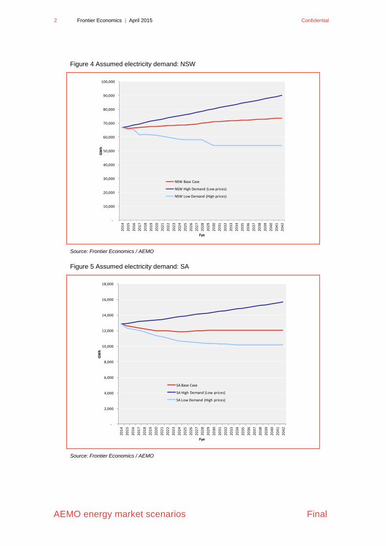
2.2 Demand
Figure 3 to Figure 7 show assumed electricity demand by state and by scenario.
In each state, the high, medium (base) and low reflects the corresponding
scenario in the 2014 NEFR:
“High demand” reflects the 2014 NEFR Scenario 2,
“Base demand” reflects the 2014 NEFR Scenario 3 (planning); and
“Low demand” reflects the 2014 NEFR Scenario 6.
These estimates reflect the original 2014 NEFR, not the December 2014 updates
released by AEMO. However, the purpose of the demand input assumption is to
reflect a starting point for the price forecasts that will be consistent with the likely
output demand forecasts from the 2015 NEFR. The 2014 NEFR scenarios
should reflect this.
Figure 3 Assumed electricity demand: QLD
Source: Frontier Economics / AEMO
-
10,000
20,000
30,000
40,000
50,000
60,000
70,000
80,000
20
14
20
15
20
16
20
17
20
18
20
19
20
20
20
21
20
22
20
23
20
24
20
25
20
26
20
27
20
28
20
29
20
30
20
31
20
32
20
33
20
34
20
35
20
36
20
37
20
38
20
39
20
40
20
41
20
42
GW
h
Fye
QLD Base Case
QLD High Demand (Low prices)
QLD Low Demand (High prices)
2 Frontier Economics | April 2015 Confidential
AEMO energy market scenarios Final
Figure 4 Assumed electricity demand: NSW
Source: Frontier Economics / AEMO
Figure 5 Assumed electricity demand: SA
Source: Frontier Economics / AEMO
-
10,000
20,000
30,000
40,000
50,000
60,000
70,000
80,000
90,000
100,000
20
14
20
15
20
16
20
17
20
18
20
19
20
20
20
21
20
22
20
23
20
24
20
25
20
26
20
27
20
28
20
29
20
30
20
31
20
32
20
33
20
34
20
35
20
36
20
37
20
38
20
39
20
40
20
41
20
42
GW
h
Fye
NSW Base Case
NSW High Demand (Low prices)
NSW Low Demand (High prices)
-
2,000
4,000
6,000
8,000
10,000
12,000
14,000
16,000
18,000
20
14
20
15
20
16
20
17
20
18
20
19
20
20
20
21
20
22
20
23
20
24
20
25
20
26
20
27
20
28
20
29
20
30
20
31
20
32
20
33
20
34
20
35
20
36
20
37
20
38
20
39
20
40
20
41
20
42
GW
h
Fye
SA Base Case
SA High Demand (Low prices)
SA Low Demand (High prices)

Confidential April 2015 | Frontier Economics 3
Final AEMO energy market scenarios
Figure 6 Assumed electricity demand: VIC
Source: Frontier Economics / AEMO
Figure 7 Assumed electricity demand: TAS
Source: Frontier Economics / AEMO
-
10,000
20,000
30,000
40,000
50,000
60,000
70,000
20
14
20
15
20
16
20
17
20
18
20
19
20
20
20
21
20
22
20
23
20
24
20
25
20
26
20
27
20
28
20
29
20
30
20
31
20
32
20
33
20
34
20
35
20
36
20
37
20
38
20
39
20
40
20
41
20
42
GW
h
Fye
VIC Base Case
VIC High Demand (Low prices)
VIC Low Demand (High prices)
-
2,000
4,000
6,000
8,000
10,000
12,000
20
14
20
15
20
16
20
17
20
18
20
19
20
20
20
21
20
22
20
23
20
24
20
25
20
26
20
27
20
28
20
29
20
30
20
31
20
32
20
33
20
34
20
35
20
36
20
37
20
38
20
39
20
40
20
41
20
42
GW
h
Fye
TAS Base Case
TAS High Demand (Low prices)
TAS Low Demand (High prices)

4 Frontier Economics | April 2015 Confidential
AEMO energy market scenarios Final
2.3 Carbon price
Figure 8 summarises the assumed carbon price by scenario. All scenarios assume
that the carbon price is replaced by Direct Action from July 2014 (starting in
FYe2015). It is assumed that the practical impact of Direct Action on the
electricity sector will be no net impact on electricity prices. This is based on the
stated principles of Direct Action that funding of abatement be sourced from the
Emissions Reduction Fund (ERF) as opposed to consumers, and that price
effects on electricity will be reduced.2 After 2020 it is assumed that some form of
carbon cost is reintroduced, in line with AEMO’s scenario assumptions.
Figure 8 Assumed carbon price by scenario
Pre 2020 - All scenarios assume carbon price is removed at the end of FYe2014, and the impact of Direct
Action is zero net effect on prices. Post 2020 - Medium: Based on EUA forward prices (EU ETS) from the
EEX High: Based on CER forward prices (CDM) from the EEX
(http://www.eex.com/en/Market%20Data/Trading%20Data/Emission%20Rights/European%20Carbon%20F
utures%20%7C%20Derivatives) Low: Based on Commonwealth Treasury forecasts from Strong Growth,
Low Pollution (Core 550ppm case).
Source: Frontier Economics
2 This is not necessarily the same as no impact on electricity sector emissions (or generators) but the
purpose of this modelling is to understand the impact on prices.
$0
$10
$20
$30
$40
$50
$60
$70
$80
$90
$100
20
14
20
15
20
16
20
17
20
18
20
19
20
20
20
21
20
22
20
23
20
24
20
25
20
26
20
27
20
28
20
29
20
30
20
31
20
32
20
33
20
34
20
35
20
36
20
37
20
38
20
39
20
40
Car
bo
n p
rice
$/t
CO
2e
(re
al 2
01
2)
Fye
Medium
High demand
Low demand
Confidential April 2015 | Frontier Economics 5
Final AEMO energy market scenarios
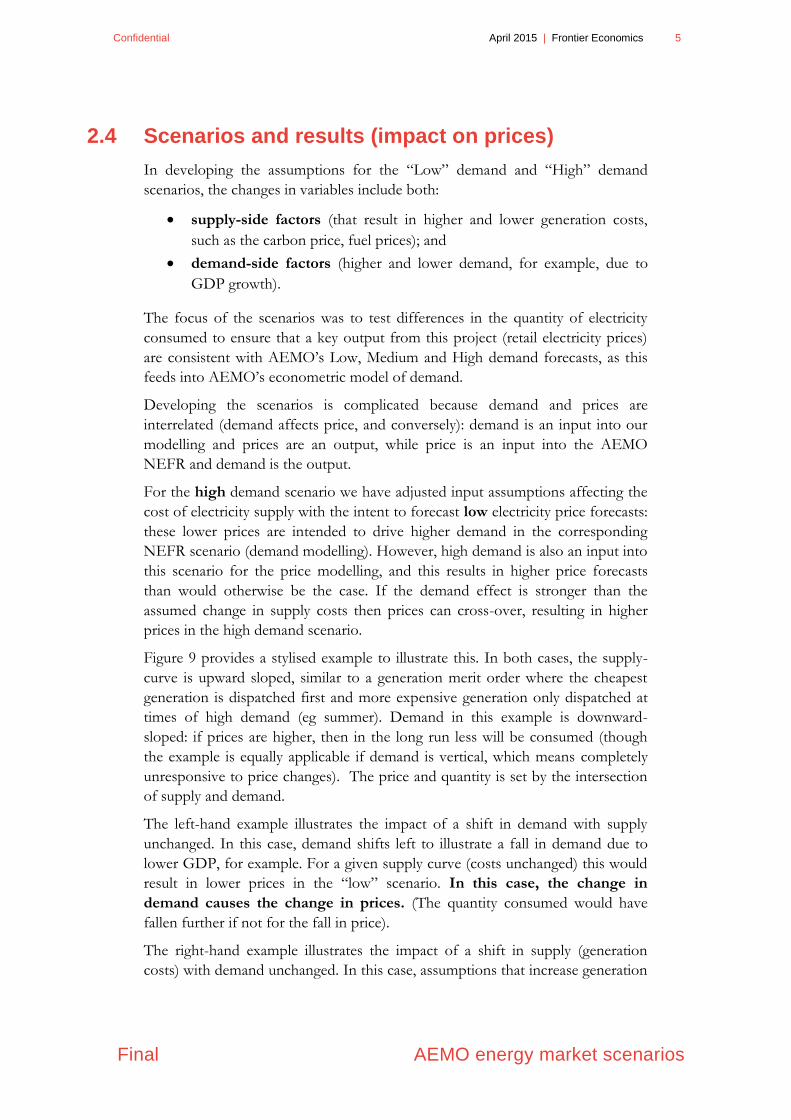
2.4 Scenarios and results (impact on prices)
In developing the assumptions for the “Low” demand and “High” demand
scenarios, the changes in variables include both:
supply-side factors (that result in higher and lower generation costs,
such as the carbon price, fuel prices); and
demand-side factors (higher and lower demand, for example, due to
GDP growth).
The focus of the scenarios was to test differences in the quantity of electricity
consumed to ensure that a key output from this project (retail electricity prices)
are consistent with AEMO’s Low, Medium and High demand forecasts, as this
feeds into AEMO’s econometric model of demand.
Developing the scenarios is complicated because demand and prices are
interrelated (demand affects price, and conversely): demand is an input into our
modelling and prices are an output, while price is an input into the AEMO
NEFR and demand is the output.
For the high demand scenario we have adjusted input assumptions affecting the
cost of electricity supply with the intent to forecast low electricity price forecasts:
these lower prices are intended to drive higher demand in the corresponding
NEFR scenario (demand modelling). However, high demand is also an input into
this scenario for the price modelling, and this results in higher price forecasts
than would otherwise be the case. If the demand effect is stronger than the
assumed change in supply costs then prices can cross-over, resulting in higher
prices in the high demand scenario.
Figure 9 provides a stylised example to illustrate this. In both cases, the supply-
curve is upward sloped, similar to a generation merit order where the cheapest
generation is dispatched first and more expensive generation only dispatched at
times of high demand (eg summer). Demand in this example is downward-
sloped: if prices are higher, then in the long run less will be consumed (though
the example is equally applicable if demand is vertical, which means completely
unresponsive to price changes). The price and quantity is set by the intersection
of supply and demand.
The left-hand example illustrates the impact of a shift in demand with supply
unchanged. In this case, demand shifts left to illustrate a fall in demand due to
lower GDP, for example. For a given supply curve (costs unchanged) this would
result in lower prices in the “low” scenario. In this case, the change in
demand causes the change in prices. (The quantity consumed would have
fallen further if not for the fall in price).
The right-hand example illustrates the impact of a shift in supply (generation
costs) with demand unchanged. In this case, assumptions that increase generation

6 Frontier Economics | April 2015 Confidential
AEMO energy market scenarios Final
costs will shift the supply-curve left: this will result in lower quantity, but this
results in higher prices. These higher prices are driven by the supply side: in this
case, the change in prices causes the change in demand.
The net effect is that prices may be higher or lower in the “Low demand”
scenario, depending on whether demand or supply-side factors dominate.
The design of our scenarios for the 2015 modelling and report has intended to
emphasise the supply-side effects to overcome any demand-side effects, so that
high energy prices feed into the Low demand scenario, and conversely.
Figure 9 Electricity prices: stylised demand-side versus supply-side factors
P = price, Q = quantity, L = low, M = medium
Source: Frontier Economics
Q:M Quantity
Price / cost
Demand: M
Supply: M
2. Market price (as a result of demand shift)
Shift in Demand (for a given Supplycurve): Low demand causes low prices,
and conversely
Demand: L
1. Demand shifts (eg due to GDP)
Q:L
P:L
Price lower in “Low”
Scenario (demand effects
dominate)
P:M
Price / cost
Demand: M
Q: M
Supply: M
2. Market price (as a result of supply shift)
Q:L
Supply: L
Shift in Supply (for a given Demand curve): Prices higher due to higher costs: High price causes Low demand (Q), and conversely
P:L
P:M
Price higher in “Low”
scenario (supply effects
dominate - prices are higher due to
higher costs, despite lower
demand)
1. Supply shifts (eg change in carbon price,
plant closure)

Confidential April 2015 | Frontier Economics 7
Final Retail electricity forecasts to 2039/40
3 Retail electricity forecasts to 2039/40
This section presents forecasts for retail electricity prices in each NEM state until
2039/40. The modelling methodology is described in Appendix A. Results are
discussed in general in section 3.1 (overview). The subsections that follow
provide more detailed state results, including:
a summary of results by state, including comparisons with historical price
estimates,
a discussion of the components of results, divided by wholesale costs,
transmission, distribution, green (LRET, SRES and other state based
schemes). This includes estimates of the contribution of each component to
projected price changes until 2020; and
comparisons with alternate sources and projections for each state, including
NIEIR’s prior projections for AEMO (2012, 2013) and AEMC estimates of
residential retail price trends from 2012, 2013 and 2014 (which review and
summarise each state regulatory determination and policy).
In most cases, the key methodologies and drivers of results/differences
between scenarios largely the same for each state. However, to enable
readers to review each state sub-section as standalone, the explanations
are provided (and repeated where applicable) in full.
3.1 Overview
This sub-section discusses general methodology and results, including:
the gathering of historical price estimates; and
a summary of residential results by region (medium case).
3.2 Historical prices
Estimates of historical prices are required as these are used in an econometric
model of demand. There is no consistent dataset that reflects absolute prices in
c/kWh (as opposed to an index) that covers the entire period 1980-2014. Various
sources available include:
ABS CPI for electricity3: This is available for the entire time period, but
only in index terms.
ESAA Electricity prices in Australia (various years): this is available in
c/kWh, but only until 2003 at the latest.
3 ABS 2013 Sep CPI release document 640108, Table 11.

8 Frontier Economics | April 2015 Confidential
Retail electricity forecasts to 2039/40 Final
AEMC 2012, 20134 and 2014: the AEMC estimated Standing Offer and
Market prices for residential retail in 2012 and in 2013, largely based on
regulated determinations by state. These reflect c/kWh but do not include
prior years.
These three data sources can be combined to develop a price path for the entire
period (1980-2014). For example, ESAA data from 2003 (or from 1980) can be
rolled forward at CPI to 2014, or AEMC data can be rolled back at CPI to 1980.
If the ESAA and ABS CPI data are consistent between 1980-2003 then results
rolled forward from 1980 (at CPI) should be the same as results rolled forward
from 2003. Similarly, we can compare the ESAA data from 2003 rolled forward
at CPI against the AEMC data from 2014 rolled back at CPI. In some cases there
are minor differences (CPI implies higher prices than ESAA, or vice versa).
Across all states, the 2014 AEMC prices (rolled back at ABS CPI for electricity in
that State) appear consistent with historical ESAA data. The comparisons of
results by source are provided in each State sub-section.
3.3 Summary results (residential, medium case)
Figure 10 presents the estimated historical residential prices against our
projections for each state for the Medium scenario, as a real index. The following
key results are evident:
Historically, residential prices had been relatively flat in real terms until
around 2007;
Prices increased rapidly from 2007-2014, largely due to rising network costs;
A further increase is evident in FYe2013, when the carbon price was
introduced. However prices also fell from FYe2014 to FYe2015 with the
removal of the carbon price.
Projected wholesale prices are relatively flat for several years before rising in
the longer term. This is due to the following reasons:
● Currently, wholesale prices are very low. This is due to weak demand and
a ramping up of renewable investment to meet the renewable energy
target (LRET), which contributes to oversupply;
4 AEMC 2013 refers to 2013 Residential Price Trends, Dec 2013
http://www.aemc.gov.au/Media/docs/2013-Residential-Electricity-Price-Trends-Final-Report-723596d1-fe66-43da-aeb6-1ee16770391e-0.PDF AEMC 2012 refers to Possible future retail electricity price movements: 1 July 2012 to 30 June 2015, Mar 2013, http://www.aemc.gov.au/Media/docs/ELECTRICITY-PRICE-TRENDS-FINAL-REPORT-609e9250-31cb-4a22-8a79-60da9348d809-0.PDF AEMC 2014 refers to: http://www.aemc.gov.au/getattachment/ae5d0665-7300-4a0d-b3b2-bd42d82cf737/2014-Residential-Electricity-Price-Trends-report.aspx

Confidential April 2015 | Frontier Economics 9
Final Retail electricity forecasts to 2039/40
● As demand eventually recovers, the demand/supply balance is expected
to tighten. This does not require rising demand in all states/markets:
demand is generally expected to rise in Qld, NSW and Vic (larger
markets) and due to interconnection of regions, this is likely to affect
demand/prices in other NEM regions (the regions with faster growing
demand will tend to export less from, or import more to, other regions);
● Gas prices are projected to rise over time, contributing to higher
generation costs. This is largely driven by the introduction of export
LNG markets in the eastern states in Qld from around 2015. This rising
gas cost particularly drives results around 2030 as the demand/supply
balance tightens in the NEM;
● After the initial removal of the carbon prices (which contributes to the
initial fall), this is assumed to contribute once again to rising prices post-
2020;
In NSW, network costs fall sharply in 2016 in line with the recent AER Draft
Determinations. Draft determinations are not yet available for other regions
(for the next regulatory period) and the NSP proposals that are available do
not include similar reductions in network costs.
We assume that the LRET ends in 2030, and this causes a dip in most
regions in 2031 (due to lower green costs). This dip also occurs in Tas,
though it is less evident due to a small rise in wholesale costs in that year.
Figure 10: Electricity: residential retail, all states, Real index, Medium case
Source: Frontier Economics
0.00
0.20
0.40
0.60
0.80
1.00
1.20
1.40
1.60
1.80
19
81
19
83
19
85
19
87
19
89
19
91
19
93
19
95
19
97
19
99
20
01
20
03
20
05
20
07
20
09
20
11
20
13
20
15
20
17
20
19
20
21
20
23
20
25
20
27
20
29
20
31
20
33
20
35
20
37
20
39
20
41
Re
al in
de
x (
20
12
=1
)
QLD
NSW
VIC
SA
TAS
Forecast Historical

10 Frontier Economics | April 2015 Confidential
Retail electricity forecasts to 2039/40 Final
3.4 Queensland
3.4.1 Historical: residential
Figure 11 shows an estimate of the historical retail residential electricity price in
Qld, applying different methodologies and sources. In Qld, prices were relatively
steady (in nominal terms) until around 2000, but have escalated rapidly since
then, particularly over the past 6-7 years as network costs have risen.
Figure 11 Electricity: Historical residential retail, Qld, nominal c/kWh
Source: CPI refers to state electricity CPI from ABS 2014 Sep CPI release document 640108, Table 11. ESAA Electricity Prices in Australia (various years). AEMC 2013 refers to 2013 Residential Price Trends, Dec 2013 http://www.aemc.gov.au/Media/docs/2013-Residential-Electricity-Price-Trends-Final-Report-723596d1-fe66-43da-aeb6-1ee16770391e-0.PDF AEMC 2012 refers to Possible future retail electricity price movements: 1 July 2012 to 30 June 2015, Mar 2013, http://www.aemc.gov.au/Media/docs/ELECTRICITY-PRICE-TRENDS-FINAL-REPORT-609e9250-31cb-4a22-8a79-60da9348d809-0.PDF. AEMC 2014 refers to: http://www.aemc.gov.au/getattachment/ae5d0665-7300-4a0d-b3b2-bd42d82cf737/2014-Residential-Electricity-Price-Trends-report.aspx
0
20
40
60
80
100
120
0.0
5.0
10.0
15.0
20.0
25.0
30.0
35.0
19
80
19
81
19
82
19
83
19
84
19
85
19
86
19
87
19
88
19
89
19
90
19
91
19
92
19
93
19
94
19
95
19
96
19
97
19
98
19
99
20
00
20
01
20
02
20
03
20
04
20
05
20
06
20
07
20
08
20
09
20
10
20
11
20
12
20
13
20
14
Re
tail
resi
de
nti
al (
no
min
al c
/kW
h)
FYe
ESAA to 2003, CPI to 2014
AEMC 2012 as base, rolled back at CPI
AEMC 2013 (midpoint of SO and market, rolled back at CPI)
AEMC 2013 Market
AEMC 2014 Representative offer, rolled back at CPI

Confidential April 2015 | Frontier Economics 11
Final Retail electricity forecasts to 2039/40
3.4.2 Historical: Business
Figure 12 compares this estimate of business electricity prices against residential.
These were relatively similar (in nominal terms) from 1995-2000 but have
diverged significantly since 2000 as residential prices have risen more rapidly.
Figure 12 Electricity: Historical business and residential retail, Qld, nominal c/kWh
Source: CPI refers to state electricity CPI from ABS 2014Sep CPI release document 640108, Table 11.
ESAA Electricity Prices in Australia (various years). PPI refers to ABS 6427.0 Producer Price Indexes,
Australia, Table 13. (electricity). AEMC 2014 refers to: http://www.aemc.gov.au/getattachment/ae5d0665-
7300-4a0d-b3b2-bd42d82cf737/2014-Residential-Electricity-Price-Trends-report.aspx
3.4.3 Results: comparisons of scenarios
Figure 13 presents the historical residential prices against our projections for each
scenario as a real index. The following key results are evident:
Historically, residential prices had been flat (or falling) in real terms until
around 2007;
Prices increased rapidly from 2007-2014, largely due to rising network costs;
A further increase is evident in FYe2013 when the carbon price was
introduced though prices fell from FYe2014 to FYe2015 due to the removal
of the carbon price.
0.0
5.0
10.0
15.0
20.0
25.0
30.0
35.0
19
80
19
81
19
82
19
83
19
84
19
85
19
86
19
87
19
88
19
89
19
90
19
91
19
92
19
93
19
94
19
95
19
96
19
97
19
98
19
99
20
00
20
01
20
02
20
03
20
04
20
05
20
06
20
07
20
08
20
09
20
10
20
11
20
12
20
13
20
14
Re
tail
ele
ctri
city
(no
min
al c
/kW
h)
FYe
Business: ESAA Business to 2003, PPI to 2014
Residential: AEMC 2014 Representative offer, rolled back at CPI

12 Frontier Economics | April 2015 Confidential
Retail electricity forecasts to 2039/40 Final
In the Medium and Low scenarios, projected retail prices begin to rise in real
terms from 2016 as increases in network costs offset the initial fall in
wholesale costs once carbon is removed.
Currently, wholesale prices are very low. This is due to weak demand growth
and a ramping up of renewable investment to meet the renewable energy
target (LRET);
● As demand eventually recovers the demand/supply balance can be
expected to tighten;
● Gas prices are projected to rise over time, contributing to higher
generation costs. This is largely driven by the introduction of export
LNG markets in the eastern states in Qld from around 2015;
● After the removal of the carbon prices (which contributed to a fall in
wholesale cost from FYe2014-2015), this is expected to contribute once
again to rising prices post-2020.
Comparing the different scenarios:
● Section 2.4 explains that prices may be higher or lower in the “Low
demand” scenario, depending on whether demand or supply-side factors
dominate. Low demand will cause lower prices, but higher supply costs in
the Low scenario will cause higher prices (which in turn should cause
lower demand).
● In the scenarios modelled, supply-side effects are expected to
dominate in the short and long-run. The “Low” demand scenario
includes higher cost estimates, and this flows through to higher retail
prices then the other scenarios, despite the lower demand in that scenario.
Similarly, the “High” demand scenario has lower cost assumptions and
these supply-side factors drive lower projected prices in the long-run,
despite the higher-demand assumption.
● The high demand sensitivity does result in higher wholesale cost
projections than in the Medium/Base case, however this is more than
offset by differences in network cost assumptions between the scenarios.
In the High demand case, network costs are assumed to fall by a similar
amount to the AER Draft Determinations for NSW, hence retail price
forecasts in the High Demand case are consistently lower than the
Medium Demand case.

Confidential April 2015 | Frontier Economics 13
Final Retail electricity forecasts to 2039/40
Figure 13 Electricity: residential retail by case, Qld (Real index)
Source: Frontier Economics
Figure 14 Electricity: business retail by case, Qld (Real index)
Source: Frontier Economics
0.00
0.50
1.00
1.50
2.00
2.50
19
81
19
84
19
87
19
90
19
93
19
96
19
99
20
02
20
05
20
08
20
11
20
14
20
17
20
20
20
23
20
26
20
29
20
32
20
35
20
38
20
41
Re
al in
de
x (2
02
12
= 1
) Base
Historical
Low demand
High Demand
0.00
0.50
1.00
1.50
2.00
2.50
19
81
19
84
19
87
19
90
19
93
19
96
19
99
20
02
20
05
20
08
20
11
20
14
20
17
20
20
20
23
20
26
20
29
20
32
20
35
20
38
20
41
Re
al in
de
x (2
02
12
= 1
) Base
Historical
Low demand
High Demand
14 Frontier Economics | April 2015 Confidential
Retail electricity forecasts to 2039/40 Final
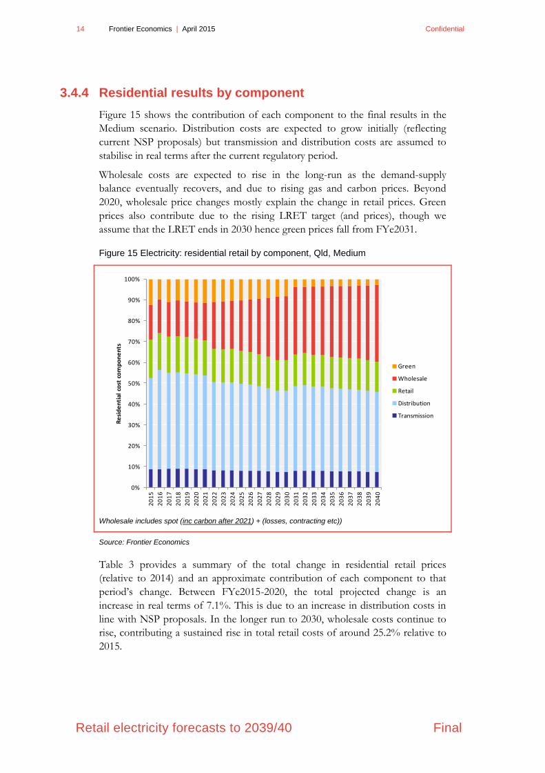
3.4.4 Residential results by component
Figure 15 shows the contribution of each component to the final results in the
Medium scenario. Distribution costs are expected to grow initially (reflecting
current NSP proposals) but transmission and distribution costs are assumed to
stabilise in real terms after the current regulatory period.
Wholesale costs are expected to rise in the long-run as the demand-supply
balance eventually recovers, and due to rising gas and carbon prices. Beyond
2020, wholesale price changes mostly explain the change in retail prices. Green
prices also contribute due to the rising LRET target (and prices), though we
assume that the LRET ends in 2030 hence green prices fall from FYe2031.
Figure 15 Electricity: residential retail by component, Qld, Medium
Wholesale includes spot (inc carbon after 2021) + (losses, contracting etc))
Source: Frontier Economics
Table 3 provides a summary of the total change in residential retail prices
(relative to 2014) and an approximate contribution of each component to that
period’s change. Between FYe2015-2020, the total projected change is an
increase in real terms of 7.1%. This is due to an increase in distribution costs in
line with NSP proposals. In the longer run to 2030, wholesale costs continue to
rise, contributing a sustained rise in total retail costs of around 25.2% relative to
2015.
0%
10%
20%
30%
40%
50%
60%
70%
80%
90%
100%
20
15
20
16
20
17
20
18
20
19
20
20
20
21
20
22
20
23
20
24
20
25
20
26
20
27
20
28
20
29
20
30
20
31
20
32
20
33
20
34
20
35
20
36
20
37
20
38
20
39
20
40
Re
sid
en
tial
co
st c
om
po
ne
nts
Green
Wholesale
Retail
Distribution
Transmission

Confidential April 2015 | Frontier Economics 15
Final Retail electricity forecasts to 2039/40
Table 3 Price change and contribution by component, Qld, real $ (Medium)
Source of change by component
(contribution to total)
Total Comment
FYe Trans Dist. Green Retail Whole-
sale
2014-
2020 0.8% 4.7% -0.4% 0.1% 1.9% 7.1%
Real prices are forecast to increase from 2015-
2020, mostly due to rising network costs
(particularly from 2015 to 2016 based on NSP
proposals). Wholesale costs are projected to
remain relatively flat in the short term (after the
removal of the carbon price) due to slow
demand growth and the ramping up of the RET
(which leads to excess supply and mitigates
price increases). Green costs are expected to
remain relatively flat in Qld: despite the ramping
up of the RET, costs from the solar bonus
scheme are expected to fall.
2014-
2030 0.8% 4.7% -2.0% 0.1% 21.6% 25.2%
Real prices are forecast to increase by around
25% from 2015-2030. The contribution of
network costs to this increase mostly occurs in
the short term. In the longer term, the biggest
contributing factor is projected to be increases in
wholesale costs, mostly after 2020. This is due
to tightening supply-demand balance as
demand recovers and the RET flattens out.
Other factors contributing to the wholesale cost
increases are rising fuel costs (gas and coal)
and the assumed reintroduction of some form of
carbon cost. Green costs stabilise from 2020-
2030 as the RET flattens out, and these costs
reduce after 2030 as the RET is assumed to end
in that year.
Source: Frontier Economics. Note: the source of change by component reflects the percentage contribution
to the change in total price (such that the sum of each component adds to the total change. Carbon costs
are reflected in wholesale costs.
Figure 16 and Figure 17 show the price forecasts for the Low (and High) demand
scenarios by component. Rising (falling) network costs are a key driver in these
sensitivities. In particular, in the High demand scenario the network costs are
assumed to fall from 2015/16 by a similar amount to the AER determination in
NSW.

16 Frontier Economics | April 2015 Confidential
Retail electricity forecasts to 2039/40 Final
Figure 16 Electricity: residential retail by component, Qld, Low demand
Wholesale includes spot (inc carbon) + (losses, contracting etc).
Source: Frontier Economics
Figure 17 Electricity: residential retail by component, Qld, High demand
Wholesale includes spot (inc carbon) + (losses, contracting etc).
Source: Frontier Economics
0%
10%
20%
30%
40%
50%
60%
70%
80%
90%
100%
20
15
20
16
20
17
20
18
20
19
20
20
20
21
20
22
20
23
20
24
20
25
20
26
20
27
20
28
20
29
20
30
20
31
20
32
20
33
20
34
20
35
20
36
20
37
20
38
20
39
20
40
Re
sid
en
tial
co
st c
om
po
ne
nts
Green
Wholesale
Retail
Distribution
Transmission
0%
10%
20%
30%
40%
50%
60%
70%
80%
90%
100%
20
15
20
16
20
17
20
18
20
19
20
20
20
21
20
22
20
23
20
24
20
25
20
26
20
27
20
28
20
29
20
30
20
31
20
32
20
33
20
34
20
35
20
36
20
37
20
38
20
39
20
40
Re
sid
en
tial
co
st c
om
po
ne
nts
Green
Wholesale
Retail
Distribution
Transmission

Confidential April 2015 | Frontier Economics 17
Final Retail electricity forecasts to 2039/40
3.4.5 Comparisons: alternate sources
Figure 18 presents a comparison of current and previous energy price projections
used as inputs into AEMO’s demand forecasts, as real indices rebased to
2012=100. The 2015 Frontier projections reflect more recent information
regarding NSP proposals for network costs (a small increase), and changes to the
solar bonus scheme. This results in higher interim forecasts than in 2014 (from
2017-2030). In the longer-run (post 2030) the higher network costs in the 2015
forecasts are offset by an updated assumption regarding the end of the LRET
scheme in 2030 which results in a dip in the index in 2031 in the latest forecast
(converging on the 2014 forecast). The current LRET legislation has the target
ending in 2030 and we have assumed that this will not be extended, hence LRET
costs are expected to fall to zero from 2031 in line with the end of the scheme.
For the 2014 forecasts we implicitly assumed that the target would be extended
to enable renewable projects built from 2020 onwards to earn more than ten
years of LGC revenue (to better reflect project life spans).
Figure 18 Electricity: residential retail, Qld, real index, compared with previous
projections
Source: NIEIR 2012: Medium scenario from
http://www.aemo.com.au/Electricity/Planning/Forecasting/National-Electricity-Forecasting-Report-
2012/~/media/Files/Other/forecasting/NIEIR%20Final%20Data%20for%20AEMO.ashx NIEIR 2013:
Medium scenario from http://www.aemo.com.au/Electricity/Planning/Forecasting/National-Electricity-
Forecasting-Report-2013/~/media/Files/Other/planning/NEFR/2013/NIEIR_EVIEWS_2013.xlsx.ashx.
0
0.2
0.4
0.6
0.8
1
1.2
1.4
1.6
1.8
19
81
19
83
19
85
19
87
19
89
19
91
19
93
19
95
19
97
19
99
20
01
20
03
20
05
20
07
20
09
20
11
20
13
20
15
20
17
20
19
20
21
20
23
20
25
20
27
20
29
20
31
20
33
20
35
20
37
20
39
Re
al n
de
x (2
01
2 b
ase
)
NIEIR 2012 (Rebased to 2012 index)
NIEIR 2013 (Rebased to 2012 index)
Frontier (2014 Medium)
Frontier (2015 Medium)

18 Frontier Economics | April 2015 Confidential
Retail electricity forecasts to 2039/40 Final
3.5 NSW and ACT
3.5.1 Historical: residential
Figure 19 shows an estimate of the historical retail residential electricity price in
NSW, applying different methodologies and sources. In NSW price were
relatively steady (in nominal terms) until around 2000, but have escalated rapidly
since then, particularly over the past 6-7 years as network costs have risen.
Figure 19 Electricity: Historical residential retail, NSW and ACT, nominal c/kWh
Source: CPI refers to state electricity CPI from ABS 2014 Sep CPI release document 640108, Table 11. ESAA Electricity Prices in Australia (various years). AEMC 2013 refers to 2013 Residential Price Trends, Dec 2013 http://www.aemc.gov.au/Media/docs/2013-Residential-Electricity-Price-Trends-Final-Report-723596d1-fe66-43da-aeb6-1ee16770391e-0.PDF AEMC 2012 refers to Possible future retail electricity price movements: 1 July 2012 to 30 June 2015, Mar 2013, http://www.aemc.gov.au/Media/docs/ELECTRICITY-PRICE-TRENDS-FINAL-REPORT-609e9250-31cb-4a22-8a79-60da9348d809-0.PDF. AEMC 2014 refers to: http://www.aemc.gov.au/getattachment/ae5d0665-7300-4a0d-b3b2-bd42d82cf737/2014-Residential-Electricity-Price-Trends-report.aspx
3.5.2 Historical: Business
Figure 20 compares this estimate of business electricity prices against residential.
These were relatively similar (in nominal terms) from 1980-2000 but have
diverged significantly since 2000 as residential prices have risen more rapidly.
0
20
40
60
80
100
120
0.0
5.0
10.0
15.0
20.0
25.0
30.0
35.0
19
80
19
81
19
82
19
83
19
84
19
85
19
86
19
87
19
88
19
89
19
90
19
91
19
92
19
93
19
94
19
95
19
96
19
97
19
98
19
99
20
00
20
01
20
02
20
03
20
04
20
05
20
06
20
07
20
08
20
09
20
10
20
11
20
12
20
13
20
14
Re
tail
resi
de
nti
al (
no
min
al c
/kW
h)
FYe
ESAA to 2003, CPI to 2014
AEMC 2012 as base, rolled back at CPI
AEMC 2013 (midpoint of SO and market, rolled back at CPI)
AEMC 2013 Market
AEMC 2014 Representative offer, rolled back at CPI

Confidential April 2015 | Frontier Economics 19
Final Retail electricity forecasts to 2039/40
Figure 20 Electricity: Historical business and residential retail, NSW and ACT,
nominal c/kWh
Source: CPI refers to state electricity CPI from ABS 2014Sep CPI release document 640108, Table 11.
ESAA Electricity Prices in Australia (various years). PPI refers to ABS 6427.0 Producer Price Indexes,
Australia, Table 13. (electricity). AEMC 2014 refers to: http://www.aemc.gov.au/getattachment/ae5d0665-
7300-4a0d-b3b2-bd42d82cf737/2014-Residential-Electricity-Price-Trends-report.aspx
3.5.3 Results: comparisons of scenarios
Figure 21 presents the historical residential prices against our projections for each
scenario as an index. The following key results are evident:
Historically, residential prices had been flat in real terms until around 2007;
Prices increased rapidly from 2007-2013, largely due to rising network costs;
A further increase is evident in FYe2013 when the carbon price was
introduced though prices fell from FYe2014 to FYe2015 due to the removal
of the carbon price.
In the Medium case, projected retail prices are relatively flat in real terms
until around 2040. This is because it takes a long time until the expected rise
in wholesale/green costs in the long run offsets the initial sharp falls due to
removing the carbon price and the AER Draft determinations on network
costs.
0.0
5.0
10.0
15.0
20.0
25.0
30.0
35.0
19
80
19
81
19
82
19
83
19
84
19
85
19
86
19
87
19
88
19
89
19
90
19
91
19
92
19
93
19
94
19
95
19
96
19
97
19
98
19
99
20
00
20
01
20
02
20
03
20
04
20
05
20
06
20
07
20
08
20
09
20
10
20
11
20
12
20
13
20
14
Re
tail
ele
ctri
city
(no
min
al c
/kW
h)
FYe
Business: ESAA Business to 2003, PPI to 2014
Residential: AEMC 2014 Representative offer, rolled back at CPI

20 Frontier Economics | April 2015 Confidential
Retail electricity forecasts to 2039/40 Final
Currently, wholesale prices are very low. This is due to weak demand growth
and a ramping up of renewable investment to meet the renewable energy
target (LRET);
● As demand eventually recovers the demand/supply balance can be
expected to tighten;
● Gas prices are projected to rise over time, contributing to higher
generation costs. This is largely driven by the introduction of export
LNG markets in the eastern states in Qld from around 2015;
● After the initial removal of the carbon prices (which contributes to the
initial fall), this is expected to contribute once again to rising prices post-
2020.
Comparing the different scenarios:
● Section 2.4 explains that prices may be higher or lower in the “Low
demand” scenario, depending on whether demand or supply-side factors
dominate. Low demand will cause lower prices, but higher supply costs in
the Low scenario will cause higher prices (which in turn should cause
lower demand).
● In the scenarios modelled, supply-side effects are expected to
dominate in the short and long-run. The “Low” demand scenario
includes higher cost estimates, and this flows through to higher retail
prices then the other scenarios, despite the lower demand in that scenario.
Similarly, the “High” demand scenario has lower cost assumptions and
these supply-side factors drive lower projected prices in the long-run,
despite the higher-demand assumption.
● The high demand sensitivity does result in higher wholesale cost
projections than in the Medium/Base case, however this is offset by
differences in network cost assumptions between the scenarios, hence
retail price forecasts in the High Demand case remain marginally lower
than the Medium Demand case. However, the variance in price
projections between these scenarios (particularly the Medium and High
demand) is less extreme than other states because the NSW Medium case
already reflects substantially lower network costs, in line with the AER
Draft Determinations.

Confidential April 2015 | Frontier Economics 21
Final Retail electricity forecasts to 2039/40
Figure 21 Electricity: residential retail by case, NSW (Real index)
Source: Frontier Economics
Figure 22 Electricity: business retail by case, NSW (Real index)
Source: Frontier Economics
0.00
0.20
0.40
0.60
0.80
1.00
1.20
1.40
1.60
1.80
19
81
19
84
19
87
19
90
19
93
19
96
19
99
20
02
20
05
20
08
20
11
20
14
20
17
20
20
20
23
20
26
20
29
20
32
20
35
20
38
20
41
Re
al in
de
x (2
02
12
= 1
) Base
Historical
Low demand
High Demand
0.00
0.20
0.40
0.60
0.80
1.00
1.20
1.40
1.60
1.80
2.00
19
81
19
84
19
87
19
90
19
93
19
96
19
99
20
02
20
05
20
08
20
11
20
14
20
17
20
20
20
23
20
26
20
29
20
32
20
35
20
38
20
41
Re
al in
de
x (2
02
12
= 1
) Base
Historical
Low demand
High Demand

22 Frontier Economics | April 2015 Confidential
Retail electricity forecasts to 2039/40 Final
3.5.4 Residential results by component
Figure 23 shows the contribution of each component to the final results in the
Medium scenario. Transmission and Distribution costs fall sharply from
FYe2015-2016, reflecting the most recent AER Draft determinations. Wholesale
costs are expected to remain relatively flat in the short term before rising in the
long-run as the demand-supply balance eventually recovers, and due to rising gas
and carbon prices in the longer run. Green costs generally rise slightly as the
LRET share increases to 2020 (which has an impact on volume and LRET
prices). Beyond 2020, wholesale price changes mostly explain the change in retail
prices.
Figure 23 Electricity: residential retail by component, NSW, Medium
Wholesale includes spot (inc carbon) + (losses, contracting etc ).
Source: Frontier Economics
Table 4 provides a summary of the total change in residential retail prices
(relative to 2015) and an approximate contribution of each component to that
period’s change. In NSW, prices are expected to fall sharply in the short term due
to falling network costs, reflecting the latest AER Draft Determinations. The
AER distribution determinations are approximately 30% lower than the NSP
proposals, due to lower OPEX and lower WACC assumptions. Beyond this,
wholesale price changes and rising green costs (LRET) largely explain changes in
the retail prices. Between FYe2015-2020, the total projected change is a fall in
real terms of 9.4%. In the longer term, wholesale costs begin to rise, reflecting
the tightening of the wholesale market supply-demand balance, rising fuel prices
0%
10%
20%
30%
40%
50%
60%
70%
80%
90%
100%
20
15
20
16
20
17
20
18
20
19
20
20
20
21
20
22
20
23
20
24
20
25
20
26
20
27
20
28
20
29
20
30
20
31
20
32
20
33
20
34
20
35
20
36
20
37
20
38
20
39
20
40
Re
sid
en
tial
co
st c
om
po
ne
nts
Green
Wholesale
Retail
Distribution
Transmission

Confidential April 2015 | Frontier Economics 23
Final Retail electricity forecasts to 2039/40
and the assumed re-introduction of some form of carbon cost. Between 2015-
2030, wholesale costs are expected to contribute to a 22.5% increase in
residential retail prices. This more than offsets the short term fall in network
costs, resulting in a projected net increase in retail prices of 10.6% between 2015-
2030.
Table 4 Price change and contribution by component, NSW, real $ (Medium)
Source of change by component
(contribution to total)
Total Comment
FYe Trans Dist. Green Retail Whole-
sale
2015-
2020 -1.4% -12.5% 2.8% 0.1% 1.7% -9.4%
Real prices are forecast to fall materially from
2015-2020. This is mostly due to a sharp fall in
distribution network costs (particularly from 2015
to 2016 based on the AER Draft
determinations). After the removal of the carbon
price at the end of FY2014, wholesale costs are
expected to remain relatively flat relatively flat to
2020 due to slow demand growth and the
ramping up of the RET (which leads to excess
supply and mitigates price increases). . Green
costs increase to 2020 in line with increases in
the RET, which peaks in 2020.
2015-
2030 -1.4% -12.5% 1.9% 0.1% 22.5% 10.6%
Real prices are forecast to rise above 2015
levels before 2030, even assuming that network
costs fall in line with the AER draft
determination. In the longer term, wholesale
costs are projected to rise due to the tightening
supply-demand balance as demand recovers
and the RET flattens out. This more than offsets
the short-term fall in network costs. Other
factors contributing to the long run increases in
wholesale costs are rising fuel costs (gas and
coal) and the assumed reintroduction of some
form of carbon cost. Green costs stabilise from
2020-2030 as the RET flattens out, and these
costs reduce after 2030 as the RET is assumed
to end in that year.
Source: Frontier Economics. Note: the source of change by component reflects the percentage contribution
to the change in total price (such that the sum of each component adds to the total change). Carbon costs
are reflected in wholesale costs.
Figure 24 and Figure 25 show the price forecasts for the Low (and High) demand
scenarios by component. Rising (falling) network costs are a key driver. However,
in the High demand scenario the assumed fall in network costs from 2015/16 are
the same as was assumed for the Medium scenario; the difference in this instance
is the long-run assumption that network costs will fall slightly in real terms over
time.

24 Frontier Economics | April 2015 Confidential
Retail electricity forecasts to 2039/40 Final
Figure 24 Electricity: residential retail by component, NSW, Low demand
Wholesale includes spot (inc carbon) + (losses, contracting etc).
Source: Frontier Economics
Figure 25 Electricity: residential retail by component, NSW, High demand
Wholesale includes spot (inc carbon) + (losses, contracting etc).
Source: Frontier Economics
0%
10%
20%
30%
40%
50%
60%
70%
80%
90%
100%
20
15
20
16
20
17
20
18
20
19
20
20
20
21
20
22
20
23
20
24
20
25
20
26
20
27
20
28
20
29
20
30
20
31
20
32
20
33
20
34
20
35
20
36
20
37
20
38
20
39
20
40
Re
sid
en
tial
co
st c
om
po
ne
nts
Green
Wholesale
Retail
Distribution
Transmission
0%
10%
20%
30%
40%
50%
60%
70%
80%
90%
100%
20
15
20
16
20
17
20
18
20
19
20
20
20
21
20
22
20
23
20
24
20
25
20
26
20
27
20
28
20
29
20
30
20
31
20
32
20
33
20
34
20
35
20
36
20
37
20
38
20
39
20
40
Re
sid
en
tial
co
st c
om
po
ne
nts
Green
Wholesale
Retail
Distribution
Transmission

Confidential April 2015 | Frontier Economics 25
Final Retail electricity forecasts to 2039/40
3.5.5 Comparisons: alternate sources
Figure 26 presents a comparison of current and previous energy price projections
used as inputs into AEMO’s demand forecasts, as real indices rebased to
2012=100. The most notable difference in the 2015 Frontier projection
(compared with 2014) is the material fall in network costs in 2016, reflecting the
AER draft determination for the next regulatory period. This results in lower
forecasts than in 2014 though out the projection period.
The 2015 forecast also reflects an updated assumption regarding the end of the
LRET scheme in 2030 which results in a dip in the index in 2031 in the latest
forecast compared with the 2014 forecast. The current legislation has the target
ending in 2030 and we have assumed that this will not be extended, hence LRET
costs are expected to fall to zero from 2031 in line with the end of the scheme.
For the 2014 forecasts we implicitly assumed that the target would be extended
to enable renewable projects built from 2020 onwards to earn more than ten
years of LGC revenue (to better reflect project life spans).
Figure 26 Electricity: residential retail, NSW, real index, compared with previous
projections
Source: NIEIR 2012: Medium scenario from
http://www.aemo.com.au/Electricity/Planning/Forecasting/National-Electricity-Forecasting-Report-
2012/~/media/Files/Other/forecasting/NIEIR%20Final%20Data%20for%20AEMO.ashx NIEIR 2013:
Medium scenario from http://www.aemo.com.au/Electricity/Planning/Forecasting/National-Electricity-
Forecasting-Report-2013/~/media/Files/Other/planning/NEFR/2013/NIEIR_EVIEWS_2013.xlsx.ashx.
0
0.2
0.4
0.6
0.8
1
1.2
1.4
1.6
19
81
19
83
19
85
19
87
19
89
19
91
19
93
19
95
19
97
19
99
20
01
20
03
20
05
20
07
20
09
20
11
20
13
20
15
20
17
20
19
20
21
20
23
20
25
20
27
20
29
20
31
20
33
20
35
20
37
20
39
Re
al n
de
x (2
01
2 b
ase
)
NIEIR 2012 (Rebased to 2012 index)
NIEIR 2013 (Rebased to 2012 index)
Frontier (2014 Medium)
Frontier (2015 Medium)
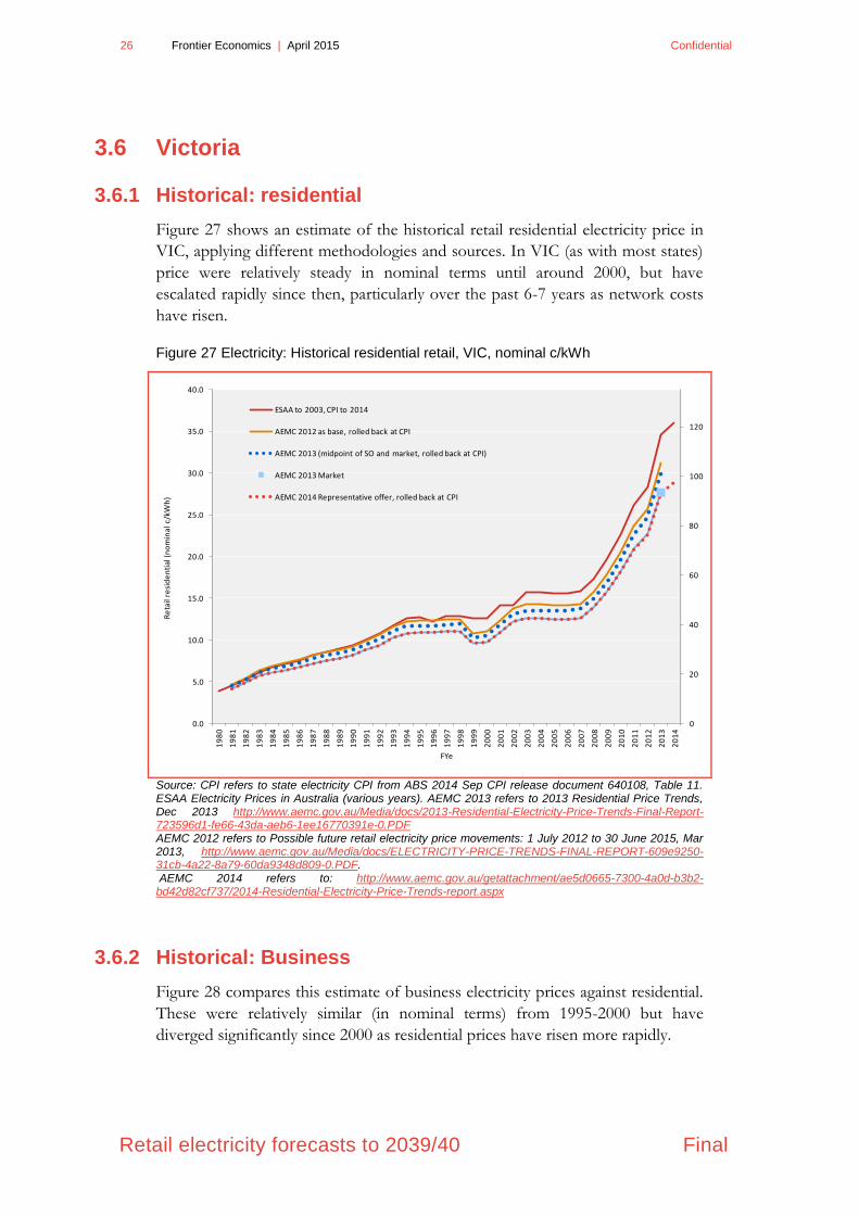
26 Frontier Economics | April 2015 Confidential
Retail electricity forecasts to 2039/40 Final
3.6 Victoria
3.6.1 Historical: residential
Figure 27 shows an estimate of the historical retail residential electricity price in
VIC, applying different methodologies and sources. In VIC (as with most states)
price were relatively steady in nominal terms until around 2000, but have
escalated rapidly since then, particularly over the past 6-7 years as network costs
have risen.
Figure 27 Electricity: Historical residential retail, VIC, nominal c/kWh
Source: CPI refers to state electricity CPI from ABS 2014 Sep CPI release document 640108, Table 11. ESAA Electricity Prices in Australia (various years). AEMC 2013 refers to 2013 Residential Price Trends, Dec 2013 http://www.aemc.gov.au/Media/docs/2013-Residential-Electricity-Price-Trends-Final-Report-723596d1-fe66-43da-aeb6-1ee16770391e-0.PDF AEMC 2012 refers to Possible future retail electricity price movements: 1 July 2012 to 30 June 2015, Mar 2013, http://www.aemc.gov.au/Media/docs/ELECTRICITY-PRICE-TRENDS-FINAL-REPORT-609e9250-31cb-4a22-8a79-60da9348d809-0.PDF. AEMC 2014 refers to: http://www.aemc.gov.au/getattachment/ae5d0665-7300-4a0d-b3b2-bd42d82cf737/2014-Residential-Electricity-Price-Trends-report.aspx
3.6.2 Historical: Business
Figure 28 compares this estimate of business electricity prices against residential.
These were relatively similar (in nominal terms) from 1995-2000 but have
diverged significantly since 2000 as residential prices have risen more rapidly.
0
20
40
60
80
100
120
0.0
5.0
10.0
15.0
20.0
25.0
30.0
35.0
40.0
19
80
19
81
19
82
19
83
19
84
19
85
19
86
19
87
19
88
19
89
19
90
19
91
19
92
19
93
19
94
19
95
19
96
19
97
19
98
19
99
20
00
20
01
20
02
20
03
20
04
20
05
20
06
20
07
20
08
20
09
20
10
20
11
20
12
20
13
20
14
Re
tail
resi
de
nti
al (
no
min
al c
/kW
h)
FYe
ESAA to 2003, CPI to 2014
AEMC 2012 as base, rolled back at CPI
AEMC 2013 (midpoint of SO and market, rolled back at CPI)
AEMC 2013 Market
AEMC 2014 Representative offer, rolled back at CPI

Confidential April 2015 | Frontier Economics 27
Final Retail electricity forecasts to 2039/40
Figure 28 Electricity: Historical business and residential retail, VIC, nominal c/kWh
Source: CPI refers to state electricity CPI from ABS 2014Sep CPI release document 640108, Table 11.
ESAA Electricity Prices in Australia (various years). PPI refers to ABS 6427.0 Producer Price Indexes,
Australia, Table 13. (electricity). AEMC 2014 refers to: http://www.aemc.gov.au/getattachment/ae5d0665-
7300-4a0d-b3b2-bd42d82cf737/2014-Residential-Electricity-Price-Trends-report.aspx
3.6.3 Results: comparisons of scenarios
● The high demand sensitivity does result in higher wholesale cost
projections than in the Medium case, however this is more than offset by
differences in network cost assumptions between the scenarios. In the
High demand case, network costs are assumed to fall by a similar amount
to the AER Draft Determinations for NSW, hence retail price forecasts in
the High Demand case are consistently lower than the Medium Demand
case.
Figure 29 presents the historical residential prices against our projections for each
scenario as an index. The following key results are evident:
Historically, residential prices had been flat in real terms until around 2007;
Prices increased rapidly from 2007-2013, largely due to rising network costs;
A further increase is evident in FYe2013 when the carbon price was
introduced though prices fell from FYe2014 to FYe2015 due to the removal
of the carbon price.
0.0
5.0
10.0
15.0
20.0
25.0
30.0
35.0
19
80
19
81
19
82
19
83
19
84
19
85
19
86
19
87
19
88
19
89
19
90
19
91
19
92
19
93
19
94
19
95
19
96
19
97
19
98
19
99
20
00
20
01
20
02
20
03
20
04
20
05
20
06
20
07
20
08
20
09
20
10
20
11
20
12
20
13
20
14
Re
tail
ele
ctri
city
(no
min
al c
/kW
h)
FYe
Business: ESAA Business to 2003, PPI to 2014
Residential: AEMC 2014 Representative offer, rolled back at CPI

28 Frontier Economics | April 2015 Confidential
Retail electricity forecasts to 2039/40 Final
In the Medium case projected retail prices dip/are relatively flat until around
2019 and then continue to rise in the longer term. This is because network
costs are expected to stabilise/flatten, but wholesale/green costs are expected
to rise.
● Currently, wholesale prices are very low. This is due to weak demand
growth and a ramping up of renewable investment to meet the renewable
energy target (LRET);
● As demand eventually recovers, the demand/supply balance can be
expected to tighten;
● Gas prices are projected to rise over time, contributing to higher
generation costs. This is driven by the introduction of export LNG
markets in the eastern states in Qld from around 2015;
● After the initial removal of the carbon prices (which contributes to the
initial fall), this is expected to contribute once again to rising prices post-
2020.
Comparing the different scenarios:
● Section 2.4 explains that prices may be higher or lower in the “Low
demand” scenario, depending on whether demand or supply-side factors
dominate. Low demand will cause lower prices, but higher supply costs
(in the Low scenario) will cause higher prices (which in turn should cause
lower demand).
● In the scenarios modelled, supply-side effects are expected to
dominate in the short and long-run. The “Low” demand scenario
includes higher cost estimates, and this flows through to higher retail
prices then the other scenarios, despite the lower demand in that scenario.
Similarly, the “High” demand scenario has lower cost assumptions and
these supply-side factors drive lower projected prices in the long-run,
despite the higher-demand assumption.
● The high demand sensitivity does result in higher wholesale cost
projections than in the Medium case, however this is more than offset by
differences in network cost assumptions between the scenarios. In the
High demand case, network costs are assumed to fall by a similar amount
to the AER Draft Determinations for NSW, hence retail price forecasts in
the High Demand case are consistently lower than the Medium Demand
case.

Confidential April 2015 | Frontier Economics 29
Final Retail electricity forecasts to 2039/40
Figure 29 Electricity: residential retail by case, VIC (Real index)
Source: Frontier Economics
Figure 30 Electricity: business retail by case, VIC (Real index)
Source: Frontier Economics
0.00
0.20
0.40
0.60
0.80
1.00
1.20
1.40
1.60
1.80
2.00
19
81
19
84
19
87
19
90
19
93
19
96
19
99
20
02
20
05
20
08
20
11
20
14
20
17
20
20
20
23
20
26
20
29
20
32
20
35
20
38
20
41
Re
al in
de
x (2
02
12
= 1
) Base
Historical
Low demand
High Demand
0.00
0.20
0.40
0.60
0.80
1.00
1.20
1.40
1.60
1.80
2.00
19
81
19
84
19
87
19
90
19
93
19
96
19
99
20
02
20
05
20
08
20
11
20
14
20
17
20
20
20
23
20
26
20
29
20
32
20
35
20
38
20
41
Re
al in
de
x (2
02
12
= 1
) Base
Historical
Low demand
High Demand

30 Frontier Economics | April 2015 Confidential
Retail electricity forecasts to 2039/40 Final
3.6.4 Residential results by component
Figure 31 shows the contribution of each component to the final results in the
Medium scenario. Prices are relatively flat from FYe2015 until around 2022.
Distribution costs are expected to rise marginally from FYe2015-2016 and then
assumed to stabilise in real terms. Wholesale costs are projected to expected to
remain relatively flat until 2020 but rise in the long-run as the demand-supply
balance eventually recovers and gas and carbon prices rise in the longer run.
Green costs generally rise slightly as the LRET share increases to 2020 (which
has an impact on volume and LRET prices). Beyond 2020, wholesale price
changes mostly explain the change in retail prices.
Figure 31 Electricity: residential retail by component, VIC, Medium
Wholesale includes spot (inc carbon) + (losses, contracting etc ).
Source: Frontier Economics
Table 5 provides a summary of the total change in residential retail prices
(relative to 2015) and an approximate contribution of each component to that
period’s change. Between FYe2015-2020, the total projected change is a rise in
real terms of 2.4%. This is mostly due to a rise in green costs. This is based on
the assumption that network costs will remain relatively stable, though at the
time of this report there were no VIC DNSP proposals (or AER Draft
determination) yet available for the next regulatory period. In the longer run to
2030, wholesale costs continue to rise due to tightening supply/demand balance
and rising fuel costs. This contributes to a sustained rise in total retail costs of
around 22.1% relative to 2015.
0%
10%
20%
30%
40%
50%
60%
70%
80%
90%
100%
20
15
20
16
20
17
20
18
20
19
20
20
20
21
20
22
20
23
20
24
20
25
20
26
20
27
20
28
20
29
20
30
20
31
20
32
20
33
20
34
20
35
20
36
20
37
20
38
20
39
20
40
Re
sid
en
tial
co
st c
om
po
ne
nts
Green
Wholesale
Retail
Distribution
Transmission

Confidential April 2015 | Frontier Economics 31
Final Retail electricity forecasts to 2039/40
Table 5 Price change and contribution by component, Vic, real $ (Medium)
Source of change by component
(contribution to total)
Total Comment
FYe Trans Dist. Green Retail Whole-
sale
2015-
2020 -0.2% 0.2% 2.1% 0.1% 0.1% 2.4%
Real prices are forecast to marginally increase
from 2014-2020. This is mostly due to an
assumed rise in network costs, and the ramping
up of the RET target, which peaks in 2020.
These increases are more than offset by falling
wholesale costs in the short term, largely due to
the removal of the carbon price. Wholesale
costs otherwise remain relatively flat to 2020
due to slow demand growth and the ramping up
of the RET (which leads to excess supply and
mitigates price increases).
2015-
2030 -0.2% 0.2% 1.0% 0.1% 21.0% 22.1%
Real prices are forecast to increase by around
12.4% from 2014-2030. The contribution of
network costs to this increase in small. In the
longer term, the biggest contributing factor is
projected to be increases in wholesale costs,
mostly after 2020. This is due to tightening
supply-demand balance as demand recovers
and the RET flattens out. Other factors
contributing to the wholesale cost increases are
rising fuel costs (gas and coal) and the assumed
reintroduction of some form of carbon cost.
Green costs stabilise from 2020-2030 as the
RET flattens out, and these costs reduce after
2030 as the RET is assumed to end in that year.
Source: Frontier Economics. Note: the source of change by component reflects the percentage contribution
to the change in total price (such that the sum of each component adds to the total change. Carbon costs
are reflected in wholesale costs.
Figure 32 and Figure 33 show the price forecasts for the Low (and High) demand
scenarios by component. Rising (falling) network costs are a key driver. However,
in the High demand scenario some of the fall in network costs is offset by
increases in expected wholesale costs as higher demand factors partly offsets the
fall in assumed supply costs.

32 Frontier Economics | April 2015 Confidential
Retail electricity forecasts to 2039/40 Final
Figure 32 Electricity: residential retail by component, VIC, Low demand
Wholesale includes spot (inc carbon) + (losses, contracting etc).
Source: Frontier Economics
Figure 33 Electricity: residential retail by component, VIC, High demand
Wholesale includes spot (inc carbon) + (losses, contracting etc ).
Source: Frontier Economics
0%
10%
20%
30%
40%
50%
60%
70%
80%
90%
100%
20
15
20
16
20
17
20
18
20
19
20
20
20
21
20
22
20
23
20
24
20
25
20
26
20
27
20
28
20
29
20
30
20
31
20
32
20
33
20
34
20
35
20
36
20
37
20
38
20
39
20
40
Re
sid
en
tial
co
st c
om
po
ne
nts
Green
Wholesale
Retail
Distribution
Transmission
0%
10%
20%
30%
40%
50%
60%
70%
80%
90%
100%
20
15
20
16
20
17
20
18
20
19
20
20
20
21
20
22
20
23
20
24
20
25
20
26
20
27
20
28
20
29
20
30
20
31
20
32
20
33
20
34
20
35
20
36
20
37
20
38
20
39
20
40
Re
sid
en
tial
co
st c
om
po
ne
nts
Green
Wholesale
Retail
Distribution
Transmission

Confidential April 2015 | Frontier Economics 33
Final Retail electricity forecasts to 2039/40
3.6.5 Comparisons: alternate sources
Figure 34 presents a comparison of current and previous energy price projections
used as inputs into AEMO’s demand forecasts, as real indices rebased to
2012=100. The 2015 Frontier projections reflect similar assumptions regarding
future network costs as 2014 and the wholesale cost forecasts are broadly similar
until 2030. Future wholesale costs post-2030 are projected to be marginally lower
than in the 2014 forecasts, reflecting updated fuel and demand assumptions.
The 2015 forecast also reflects an updated assumption regarding the end of the
LRET scheme in 2030 which results in a dip in the index in 2031 in the latest
forecast compared with the 2014 forecast. The current legislation has the target
ending in 2030 and we have assumed that this will not be extended, hence LRET
costs are expected to fall to zero from 2031 in line with the end of the scheme.
For the 2014 forecasts we implicitly assumed that the target would be extended
to enable renewable projects built from 2020 onwards to earn more than ten
years of LGC revenue (to better reflect project life spans).
Figure 34 Electricity: residential retail, VIC, real index, compared with previous
projections
Source: NIEIR 2012: Medium scenario from
http://www.aemo.com.au/Electricity/Planning/Forecasting/National-Electricity-Forecasting-Report-
2012/~/media/Files/Other/forecasting/NIEIR%20Final%20Data%20for%20AEMO.ashx NIEIR 2013:
Medium scenario from http://www.aemo.com.au/Electricity/Planning/Forecasting/National-Electricity-
Forecasting-Report-2013/~/media/Files/Other/planning/NEFR/2013/NIEIR_EVIEWS_2013.xlsx.ashx.
0
0.2
0.4
0.6
0.8
1
1.2
1.4
1.6
19
81
19
83
19
85
19
87
19
89
19
91
19
93
19
95
19
97
19
99
20
01
20
03
20
05
20
07
20
09
20
11
20
13
20
15
20
17
20
19
20
21
20
23
20
25
20
27
20
29
20
31
20
33
20
35
20
37
20
39
Re
al n
de
x (2
01
2 b
ase
)
NIEIR 2012 (Rebased to 2012 index)
NIEIR 2013 (Rebased to 2012 index)
Frontier (2014 Medium)
Frontier (2015 Medium)

34 Frontier Economics | April 2015 Confidential
Retail electricity forecasts to 2039/40 Final
3.7 South Australia
3.7.1 Historical: residential
Figure 35 shows an estimate of the historical retail residential electricity price in
SA, applying different methodologies and sources. In SA (as with most states)
price were relatively steady in nominal terms until around 2000, but have
escalated rapidly since then, particularly over the past 6-7 years as network costs
have risen.
Figure 35 Electricity: Historical residential retail, SA, nominal c/kWh
Source: CPI refers to state electricity CPI from ABS 2014 Sep CPI release document 640108, Table 11. ESAA Electricity Prices in Australia (various years). AEMC 2013 refers to 2013 Residential Price Trends, Dec 2013 http://www.aemc.gov.au/Media/docs/2013-Residential-Electricity-Price-Trends-Final-Report-723596d1-fe66-43da-aeb6-1ee16770391e-0.PDF AEMC 2012 refers to Possible future retail electricity price movements: 1 July 2012 to 30 June 2015, Mar 2013, http://www.aemc.gov.au/Media/docs/ELECTRICITY-PRICE-TRENDS-FINAL-REPORT-609e9250-31cb-4a22-8a79-60da9348d809-0.PDF. AEMC 2014 refers to: http://www.aemc.gov.au/getattachment/ae5d0665-7300-4a0d-b3b2-bd42d82cf737/2014-Residential-Electricity-Price-Trends-report.aspx
3.7.2 Historical: Business
Figure 37 compares this estimate of business electricity prices against residential.
These were relatively similar (in nominal terms) from 1995-2000 but have
diverged since 2000 as residential prices have risen more rapidly.
0
20
40
60
80
100
120
0.0
5.0
10.0
15.0
20.0
25.0
30.0
35.0
40.0
19
80
19
81
19
82
19
83
19
84
19
85
19
86
19
87
19
88
19
89
19
90
19
91
19
92
19
93
19
94
19
95
19
96
19
97
19
98
19
99
20
00
20
01
20
02
20
03
20
04
20
05
20
06
20
07
20
08
20
09
20
10
20
11
20
12
20
13
20
14
Re
tail
resi
de
nti
al (
no
min
al c
/kW
h)
FYe
ESAA to 2003, CPI to 2014
AEMC 2012 as base, rolled back at CPI
AEMC 2013 (midpoint of SO and market, rolled back at CPI)
AEMC 2013 Market
AEMC 2014 Representative offer, rolled back at CPI

Confidential April 2015 | Frontier Economics 35
Final Retail electricity forecasts to 2039/40
Figure 36 Electricity: Historical business and residential retail, SA, nominal c/kWh
Source: CPI refers to state electricity CPI from ABS 2014Sep CPI release document 640108, Table 11.
ESAA Electricity Prices in Australia (various years). PPI refers to ABS 6427.0 Producer Price Indexes,
Australia, Table 13. (electricity). AEMC 2014 refers to: http://www.aemc.gov.au/getattachment/ae5d0665-
7300-4a0d-b3b2-bd42d82cf737/2014-Residential-Electricity-Price-Trends-report.aspx
3.7.3 Results: comparisons of scenarios
Figure 37 presents the historical residential prices against our projections for each
scenario as an index. The following key results are evident:
Historically, residential prices had been flat in real terms until around 2007;
Prices increased rapidly from 2007-2013, largely due to rising network costs;
A further increase is evident in FYe2013 when the carbon price was
introduced though prices fell from FYe2014 to FYe2015 due to the removal
of the carbon price.
In general (across all scenarios) projected retail prices are relatively flat until
around 2022 and then continue to rise in the longer term. This is because
network costs are expected to stabilise/flatten, but wholesale/green costs are
expected to recover/rise in the longer term.
● Wholesale prices are currently low due to slow demand growth;
● As demand eventually recovers, the demand/supply balance can be
expected to tighten;
0.0
5.0
10.0
15.0
20.0
25.0
30.0
35.0
19
80
19
81
19
82
19
83
19
84
19
85
19
86
19
87
19
88
19
89
19
90
19
91
19
92
19
93
19
94
19
95
19
96
19
97
19
98
19
99
20
00
20
01
20
02
20
03
20
04
20
05
20
06
20
07
20
08
20
09
20
10
20
11
20
12
20
13
20
14
Re
tail
ele
ctri
city
l (n
om
inal
c/k
Wh
)
FYe
Business: ESAA Business to 2003, PPI to 2014
Residential: AEMC 2014 Representative offer, rolled back at CPI

36 Frontier Economics | April 2015 Confidential
Retail electricity forecasts to 2039/40 Final
● Gas prices are projected to rise over time, contributing to higher
generation costs. This is discussed in detail in the chapter on Gas prices,
though this is largely driven by the introduction of export LNG markets
in the eastern states in Qld from around 2015;
● After the initial removal of the carbon prices (which contributed to the
fall from FYe2014-2015), this is expected to contribute once again to
rising prices post-2020.
Comparing the different scenarios:
● Section 2.4 explains that prices may be higher or lower in the “Low
demand” scenario, depending on whether demand or supply-side factors
dominate. Low demand will cause lower prices, but higher supply costs
(in the Low scenario) will cause higher prices (which in turn should cause
lower demand).
● In the scenarios modelled, supply-side effects are expected to
dominate in the short and long-run. The “Low” demand scenario
includes higher cost estimates, and this flows through to higher retail
prices then the other scenarios, despite the lower demand in that scenario.
Similarly, the “High” demand scenario has lower cost assumptions and
these supply-side factors drive lower projected prices in the long-run,
despite the higher-demand assumption.
● The high demand sensitivity does result in higher wholesale cost
projections than in the Medium/Base case, however this is more than
offset by differences in network cost assumptions between the scenarios.
In the High demand case, network costs are assumed to fall by a similar
amount to the AER Draft Determinations for NSW, hence retail price
forecasts in the High Demand case are consistently lower than the
Medium Demand case.

Confidential April 2015 | Frontier Economics 37
Final Retail electricity forecasts to 2039/40
Figure 37 Electricity: residential retail by case, SA (Real index)
Source: Frontier Economics
Figure 38 Electricity: business retail by case, SA (Real index)
Source: Frontier Economics
0.00
0.20
0.40
0.60
0.80
1.00
1.20
1.40
1.60
1.80
19
81
19
84
19
87
19
90
19
93
19
96
19
99
20
02
20
05
20
08
20
11
20
14
20
17
20
20
20
23
20
26
20
29
20
32
20
35
20
38
20
41
Re
al in
de
x (2
02
12
= 1
) Base
Historical
Low demand
High Demand
0.00
0.20
0.40
0.60
0.80
1.00
1.20
1.40
1.60
1.80
19
81
19
84
19
87
19
90
19
93
19
96
19
99
20
02
20
05
20
08
20
11
20
14
20
17
20
20
20
23
20
26
20
29
20
32
20
35
20
38
20
41
Re
al in
de
x (2
02
12
= 1
) Base
Historical
Low demand
High Demand

38 Frontier Economics | April 2015 Confidential
Retail electricity forecasts to 2039/40 Final
3.7.4 Residential results by component
Figure 39 shows the contribution of each component to the final results in the
Medium scenario. Prices are relatively flat from FYe2015 until around 2023.
Distribution costs and wholesale costs are expected to remain relatively stable in
real terms in the short term. Wholesale costs are otherwise expected to rise in the
long-run as the demand-supply balance eventually recovers, as gas prices rise in
the longer run and as some form of carbon price is assumed to have some effect
on prices in the longer run. Green costs generally rise slightly as the LRET share
increases to 2020 (which has an impact on volume and LRET prices). Beyond
2020, wholesale price changes mostly explain the change in retail prices.
Figure 39 Electricity: residential retail by component, SA, Medium
Wholesale includes spot (inc carbon) + (losses, contracting etc).
Source: Frontier Economics
Table 6 provides a summary of the total change in residential retail prices
(relative to 2015) and an approximate contribution of each component to that
period’s change. Between FYe2015-2020, the total projected change is a slight fall
in real terms of 3.1%. This is due to a marginal fall in wholesale and distribution
costs. In the longer run to 2030, wholesale costs continue to rise due to
tightening supply/demand balance and rising fuel costs. This contributes to a
sustained rise in total retail costs of around 16.0% relative to 2015.
0%
10%
20%
30%
40%
50%
60%
70%
80%
90%
100%
20
15
20
16
20
17
20
18
20
19
20
20
20
21
20
22
20
23
20
24
20
25
20
26
20
27
20
28
20
29
20
30
20
31
20
32
20
33
20
34
20
35
20
36
20
37
20
38
20
39
20
40
Re
sid
en
tial
co
st c
om
po
ne
nts
Green
Wholesale
Retail
Distribution
Transmission

Confidential April 2015 | Frontier Economics 39
Final Retail electricity forecasts to 2039/40
Table 6 Price change and contribution by component, SA, real $ (Medium)
Source of change by component (contribution
to total)
Total Comment
FYe Trans Dist. Green Retail Whole-
sale
2015-
2020 0.4% -1.4% 0.4% 0.1% -2.5% -3.1%
Real prices are forecast to marginally fall from
2015-2020. The ramping up of the RET target
(rising green costs) is more than offset by an
initial fall in network and wholesale costs in the
short term. Wholesale costs otherwise remain
relatively flat to 2020 due to slow demand
growth and the ramping up of the RET (which
leads to excess supply and mitigates price
increases).
2015-
2030 0.4% -1.4% -1.4% 0.1% 18.4% 16.0%
Real prices are forecast to increase by around
16.0% from 2015-2030. The contribution of
network costs to this increase is small. In the
longer term, the biggest contributing factor is
projected to be increases in wholesale costs,
mostly after 2020. This is due to tightening
supply-demand balance as demand recovers
and the RET flattens out. Other factors
contributing to the wholesale cost increases are
rising fuel costs (gas and coal) and the assumed
reintroduction of some form of carbon cost.
Green costs stabilise from 2020-2030 as the
RET flattens out, and these costs reduce after
2030 as the RET is assumed to end in that year.
Source: Frontier Economics. Note: the source of change by component reflects the percentage contribution
to the change in total price (such that the sum of each component adds to the total change. Carbon costs
are reflected in wholesale costs.
Figure 40 and Figure 41 show the price forecasts for the Low (and High) demand
scenarios by component. Rising (falling) network costs are a key driver. However,
in the High demand scenario some of the fall in network costs is offset by
increases in expected wholesale costs as higher demand factors partly offsets the
fall in assumed supply costs.

40 Frontier Economics | April 2015 Confidential
Retail electricity forecasts to 2039/40 Final
Figure 40 Electricity: residential retail by component, SA, Low demand
Wholesale includes spot (inc carbon) + (losses, contracting etc).
Source: Frontier Economics
Figure 41 Electricity: residential retail by component, SA, High demand
Wholesale includes spot (inc carbon) + (losses, contracting etc).
Source: Frontier Economics
0%
10%
20%
30%
40%
50%
60%
70%
80%
90%
100%
20
15
20
16
20
17
20
18
20
19
20
20
20
21
20
22
20
23
20
24
20
25
20
26
20
27
20
28
20
29
20
30
20
31
20
32
20
33
20
34
20
35
20
36
20
37
20
38
20
39
20
40
Re
sid
en
tial
co
st c
om
po
ne
nts
Green
Wholesale
Retail
Distribution
Transmission
0%
10%
20%
30%
40%
50%
60%
70%
80%
90%
100%
20
15
20
16
20
17
20
18
20
19
20
20
20
21
20
22
20
23
20
24
20
25
20
26
20
27
20
28
20
29
20
30
20
31
20
32
20
33
20
34
20
35
20
36
20
37
20
38
20
39
20
40
Re
sid
en
tial
co
st c
om
po
ne
nts
Green
Wholesale
Retail
Distribution
Transmission

Confidential April 2015 | Frontier Economics 41
Final Retail electricity forecasts to 2039/40
3.7.5 Comparisons: alternate sources
Figure 42 presents a comparison of current and previous energy price projections
used as inputs into AEMO’s demand forecasts, as real indices rebased to
2012=100. The 2015 Frontier projections reflect broadly similar assumptions
regarding future wholesale and network costs as 2014, and the projections are
very similar until 2030. Post-2030, green costs are expected to fall in line with a
revised assumption regarding the end of the LRET in 2030 (which was not
reflected in the 2014 forecasts). The current legislation has the LRET ending in
2030 and we have assumed that this will not be extended, hence LRET costs are
expected to fall to zero from 2031 in line with the end of the scheme. For the
2014 forecasts we implicitly assumed that the target would be extended to enable
renewable projects built from 2020 onwards to earn more than ten years of LGC
revenue (to better reflect project life spans), so a similar dip was not evident.
Figure 42 Electricity: residential retail, SA, real index, compared with previous
projections
Source: NIEIR 2012: Medium scenario from
http://www.aemo.com.au/Electricity/Planning/Forecasting/National-Electricity-Forecasting-Report-
2012/~/media/Files/Other/forecasting/NIEIR%20Final%20Data%20for%20AEMO.ashx NIEIR 2013:
Medium scenario from http://www.aemo.com.au/Electricity/Planning/Forecasting/National-Electricity-
Forecasting-Report-2013/~/media/Files/Other/planning/NEFR/2013/NIEIR_EVIEWS_2013.xlsx.ashx.
0
0.2
0.4
0.6
0.8
1
1.2
1.4
19
81
19
83
19
85
19
87
19
89
19
91
19
93
19
95
19
97
19
99
20
01
20
03
20
05
20
07
20
09
20
11
20
13
20
15
20
17
20
19
20
21
20
23
20
25
20
27
20
29
20
31
20
33
20
35
20
37
20
39
Re
al n
de
x (2
01
2 b
ase
)
NIEIR 2012 (Rebased to 2012 index)
NIEIR 2013 (Rebased to 2012 index)
Frontier (2014 Medium)
Frontier (2015 Medium)
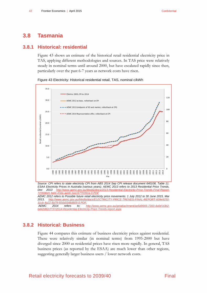
42 Frontier Economics | April 2015 Confidential
Retail electricity forecasts to 2039/40 Final
3.8 Tasmania
3.8.1 Historical: residential
Figure 43 shows an estimate of the historical retail residential electricity price in
TAS, applying different methodologies and sources. In TAS price were relatively
steady in nominal terms until around 2000, but have escalated rapidly since then,
particularly over the past 6-7 years as network costs have risen.
Figure 43 Electricity: Historical residential retail, TAS, nominal c/kWh
Source: CPI refers to state electricity CPI from ABS 2014 Sep CPI release document 640108, Table 11. ESAA Electricity Prices in Australia (various years). AEMC 2013 refers to 2013 Residential Price Trends, Dec 2013 http://www.aemc.gov.au/Media/docs/2013-Residential-Electricity-Price-Trends-Final-Report-723596d1-fe66-43da-aeb6-1ee16770391e-0.PDF AEMC 2012 refers to Possible future retail electricity price movements: 1 July 2012 to 30 June 2015, Mar 2013, http://www.aemc.gov.au/Media/docs/ELECTRICITY-PRICE-TRENDS-FINAL-REPORT-609e9250-31cb-4a22-8a79-60da9348d809-0.PDF. AEMC 2014 refers to: http://www.aemc.gov.au/getattachment/ae5d0665-7300-4a0d-b3b2-bd42d82cf737/2014-Residential-Electricity-Price-Trends-report.aspx
3.8.2 Historical: Business
Figure 44 compares this estimate of business electricity prices against residential.
These were relatively similar (in nominal terms) from 1995-2000 but have
diverged since 2000 as residential prices have risen more rapidly. In general, TAS
business prices (as reported by the ESAA) are much lower than other regions,
suggesting generally larger business users / lower network costs.
0
20
40
60
80
100
120
0.0
5.0
10.0
15.0
20.0
25.0
30.0
35.0
19
80
19
81
19
82
19
83
19
84
19
85
19
86
19
87
19
88
19
89
19
90
19
91
19
92
19
93
19
94
19
95
19
96
19
97
19
98
19
99
20
00
20
01
20
02
20
03
20
04
20
05
20
06
20
07
20
08
20
09
20
10
20
11
20
12
20
13
20
14
Re
tail
resi
de
nti
al (
no
min
al c
/kW
h)
FYe
ESAA to 2003, CPI to 2014
AEMC 2012 as base, rolled back at CPI
AEMC 2013 (midpoint of SO and market, rolled back at CPI)
AEMC 2014 Representative offer, rolled back at CPI

Confidential April 2015 | Frontier Economics 43
Final Retail electricity forecasts to 2039/40
Figure 44 Electricity: Historical business and residential retail, TAS, nominal c/kWh
Source: CPI refers to state electricity CPI from ABS 2013Sep CPI release document 640108, Table 11.
ESAA Electricity Prices in Australia (various years. AEMC 2013 refers to 2013 Residential Price Trends,
Dec 2013 http://www.aemc.gov.au/Media/docs/2013-Residential-Electricity-Price-Trends-Final-Report-
723596d1-fe66-43da-aeb6-1ee16770391e-0.PDF ‘SO’ refers to standing offer, ‘Market’ refers to market
offer. PPI refers to ABS 6427.0 Producer Price Indexes, Australia, Table 13. (electricity)
3.8.3 Results: comparisons of scenarios
Figure 43 presents the historical residential prices against our projections for each
scenario as an index. The following key results are evident:
Historically, residential prices had been flat in real terms until around 2007;
Prices increased rapidly from 2007-2013, largely due to rising network costs;
A further increase is evident in FYe2013 when the carbon price was
introduced though prices fell from FYe2014 to FYe2015 due to the removal
of the carbon price.
In general (across all scenarios) projected retail prices are relatively flat until
around 2020 and then continue to rise in the longer term. This is because
network costs are expected to fall slightly and then flatten, but
wholesale/green costs are expected to fall initially and then rise in the longer
run.
0.0
5.0
10.0
15.0
20.0
25.0
30.0
19
80
19
81
19
82
19
83
19
84
19
85
19
86
19
87
19
88
19
89
19
90
19
91
19
92
19
93
19
94
19
95
19
96
19
97
19
98
19
99
20
00
20
01
20
02
20
03
20
04
20
05
20
06
20
07
20
08
20
09
20
10
20
11
20
12
20
13
20
14
Re
tail
ele
ctri
city
(n
om
inal
c/k
Wh
)
FYe
Business: ESAA Business to 2003, PPI to 2014
Residential: AEMC 2014 Representative offer, rolled back at CPI

44 Frontier Economics | April 2015 Confidential
Retail electricity forecasts to 2039/40 Final
● Wholesale prices are currently low due to weak demand growth and a
ramping up of renewable investment to meet the renewable energy target
(LRET);
● As demand eventually recovers (and some existing plant reaches
retirement post 2020), the demand/supply balance can be expected to
tighten. This does not necessarily mean in Tasmanian (where demand
growth is still flat/falling), but demand growth in other NEM regions is
expected to contribute to prices in Tas (to the extent that energy can be
exported from Tas).
● After the initial removal of the carbon prices (which contributes to the
initial fall), this is expected to contribute once again to rising prices post-
2020.
Comparing the different scenarios:
● Section 2.4 explains that prices may be higher or lower in the “Low
demand” scenario, depending on whether demand or supply-side factors
dominate. Low demand will cause lower prices, but higher supply costs
(in the Low scenario) will cause higher prices (which in turn should cause
lower demand).
● In the scenarios modelled, supply-side effects are expected to
dominate in the short and long-run. The “Low” demand scenario
includes higher cost estimates, and this flows through to higher retail
prices then the other scenarios, despite the lower demand in that scenario.
Similarly, the “High” demand scenario has lower cost assumptions and
these supply-side factors drive lower projected prices in the long-run,
despite the higher-demand assumption.
● The high demand sensitivity does result in higher wholesale cost
projections than in the Medium/Base case, however this is more than
offset by differences in network cost assumptions between the scenarios.
In the High demand case, network costs are assumed to fall by a similar
amount to the AER Draft Determinations for NSW, hence retail price
forecasts in the High Demand case are consistently lower than the
Medium Demand case.

Confidential April 2015 | Frontier Economics 45
Final Retail electricity forecasts to 2039/40
Figure 45 Electricity: residential retail by case, TAS (Real index)
Figure 46 Electricity: business retail by case, TAS (Real index)
Source: Frontier Economics
0.00
0.20
0.40
0.60
0.80
1.00
1.20
1.40
1.60
1.80
19
81
19
84
19
87
19
90
19
93
19
96
19
99
20
02
20
05
20
08
20
11
20
14
20
17
20
20
20
23
20
26
20
29
20
32
20
35
20
38
20
41
Re
al in
de
x (2
02
12
= 1
) Base
Historical
Low demand
High Demand
0.00
0.20
0.40
0.60
0.80
1.00
1.20
1.40
1.60
1.80
2.00
19
81
19
84
19
87
19
90
19
93
19
96
19
99
20
02
20
05
20
08
20
11
20
14
20
17
20
20
20
23
20
26
20
29
20
32
20
35
20
38
20
41
Re
al in
de
x (2
02
12
= 1
) Base
Historical
Low demand
High Demand

46 Frontier Economics | April 2015 Confidential
Retail electricity forecasts to 2039/40 Final
3.8.4 Residential results by component
Figure 47 shows the contribution of each component to the final results in the
Medium scenario. Network costs are expected to fall marginally and then
assumed to stabilise in real terms. Wholesale costs are projected to remain
relatively stable (and low) in the short-term. Wholesale costs are otherwise
expected to rise in the long-run as the demand-supply balance eventually
recovers, and due to rising gas and carbon prices in the longer run5. Green costs
generally rise slightly as the LRET share increases to 2020 (which has an impact
on volume and LRET prices). Beyond 2020, wholesale price changes mostly
explain the change in retail prices. The RET is assumed to end in 2030 (as
legislated), hence the fall in green costs that year.
Figure 47 Electricity: residential retail by component, TAS, Medium
Wholesale includes spot (inc carbon) + (losses, contracting etc )
Source: Frontier Economics
Table 7 provides a summary of the total change in residential retail prices
(relative to 2015) and an approximate contribution of each component to that
period’s change. Between FYe2015-2020, the total projected change is a rise in
real terms of 1.7%. This is mostly due to the rise in green costs as the RET target
ramps up to 2020, which offsets the slight fall in network costs. In the longer run
5 It is not necessary that demand is rising in Tasmania: if prices are lower in Tasmania then exports
are likely to increase and prices between regions should tend to converge unless constraints are
binding and interconnect capacity is not expanded.
0%
10%
20%
30%
40%
50%
60%
70%
80%
90%
100%
20
15
20
16
20
17
20
18
20
19
20
20
20
21
20
22
20
23
20
24
20
25
20
26
20
27
20
28
20
29
20
30
20
31
20
32
20
33
20
34
20
35
20
36
20
37
20
38
20
39
20
40
Re
sid
en
tial
co
st c
om
po
ne
nts
Green
Wholesale
Retail
Transmission and distribution

Confidential April 2015 | Frontier Economics 47
Final Retail electricity forecasts to 2039/40
to 2030, wholesale costs continue to rise due to tightening supply/demand
balance (in Vic at least) and rising fuel costs. This contributes to a sustained rise
in total retail costs of around 20% relative to 2015.
Table 7 Price change and contribution by component, Tas, real $ (Medium)
Source of change by component
(contribution to total)
Total Comment
FYe Trans
Dist. Green Retail
Whole-
sale
2015-
2020 -2.3% 3.5% 0.0% 0.4% 1.7%
Real prices are forecast to rise marginally fall
from 2015-2020, mostly due to green costs as
the RET increases and peaks in 2020.
Wholesale costs otherwise remain relatively flat
to 2020 due to slow demand growth.
2015-
2030 -2.3% 3.2% 0.0% 19.1% 20.0%
Real prices are forecast to increase by around
20.0% from 2015-2030. In the longer term, the
contributing factors are projected to be
increases in wholesale costs (more due to
demand growth in Vic than in Tas) and mostly
after 2020. Other factors contributing to the
wholesale cost increases are rising fuel costs
(gas and coal) and the assumed reintroduction
of some form of carbon cost. Green costs
stabilise from 2020-2030 as the RET flattens
out, and these costs reduce after 2030 as the
RET is assumed to end in that year.
Source: Frontier Economics. Note: the source of change by component reflects the percentage contribution
to the change in total price (such that the sum of each component adds to the total change. Carbon costs
are reflected in wholesale costs.
Figure 48 and Figure 49 show the price forecasts for the Low (and High) demand
scenarios by component. Rising (falling) network costs are a key driver. However,
in the High demand scenario some of the fall in network costs is offset by
increases in expected wholesale costs as higher demand (in Vic) partly offsets the
fall in assumed supply costs.

48 Frontier Economics | April 2015 Confidential
Retail electricity forecasts to 2039/40 Final
Figure 48 Electricity: residential retail by component, TAS, Low demand
Wholesale includes spot (inc carbon) + (losses, contracting etc).
Source: Frontier Economics
Figure 49 Electricity: residential retail by component, TAS, High demand
Wholesale includes spot (inc carbon) + (losses, contracting etc ).
Source: Frontier Economics
0%
10%
20%
30%
40%
50%
60%
70%
80%
90%
100%
20
15
20
16
20
17
20
18
20
19
20
20
20
21
20
22
20
23
20
24
20
25
20
26
20
27
20
28
20
29
20
30
20
31
20
32
20
33
20
34
20
35
20
36
20
37
20
38
20
39
20
40
Re
sid
en
tial
co
st c
om
po
ne
nts
Green
Wholesale
Retail
Transmission and distribution
0%
10%
20%
30%
40%
50%
60%
70%
80%
90%
100%
20
15
20
16
20
17
20
18
20
19
20
20
20
21
20
22
20
23
20
24
20
25
20
26
20
27
20
28
20
29
20
30
20
31
20
32
20
33
20
34
20
35
20
36
20
37
20
38
20
39
20
40
Re
sid
en
tial
co
st c
om
po
ne
nts
Green
Wholesale
Retail
Transmission and distribution
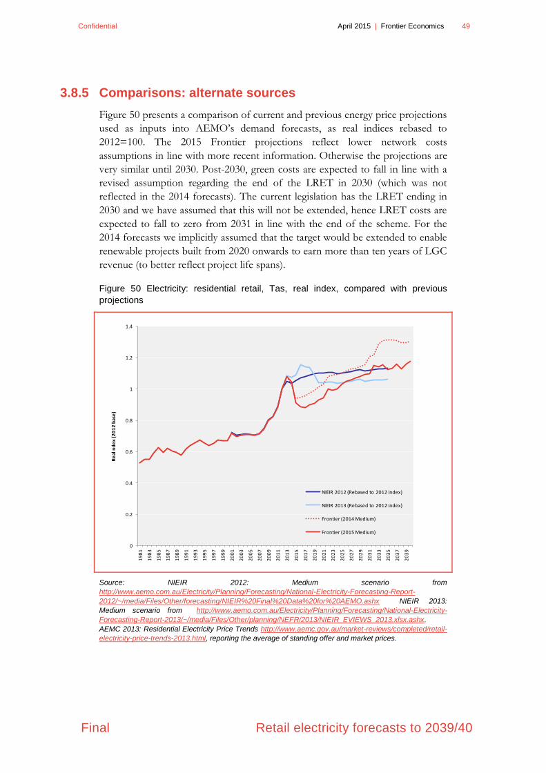
Confidential April 2015 | Frontier Economics 49
Final Retail electricity forecasts to 2039/40
3.8.5 Comparisons: alternate sources
Figure 50 presents a comparison of current and previous energy price projections
used as inputs into AEMO’s demand forecasts, as real indices rebased to
2012=100. The 2015 Frontier projections reflect lower network costs
assumptions in line with more recent information. Otherwise the projections are
very similar until 2030. Post-2030, green costs are expected to fall in line with a
revised assumption regarding the end of the LRET in 2030 (which was not
reflected in the 2014 forecasts). The current legislation has the LRET ending in
2030 and we have assumed that this will not be extended, hence LRET costs are
expected to fall to zero from 2031 in line with the end of the scheme. For the
2014 forecasts we implicitly assumed that the target would be extended to enable
renewable projects built from 2020 onwards to earn more than ten years of LGC
revenue (to better reflect project life spans).
Figure 50 Electricity: residential retail, Tas, real index, compared with previous
projections
Source: NIEIR 2012: Medium scenario from
http://www.aemo.com.au/Electricity/Planning/Forecasting/National-Electricity-Forecasting-Report-
2012/~/media/Files/Other/forecasting/NIEIR%20Final%20Data%20for%20AEMO.ashx NIEIR 2013:
Medium scenario from http://www.aemo.com.au/Electricity/Planning/Forecasting/National-Electricity-
Forecasting-Report-2013/~/media/Files/Other/planning/NEFR/2013/NIEIR_EVIEWS_2013.xlsx.ashx.
AEMC 2013: Residential Electricity Price Trends http://www.aemc.gov.au/market-reviews/completed/retail-
electricity-price-trends-2013.html, reporting the average of standing offer and market prices.
0
0.2
0.4
0.6
0.8
1
1.2
1.4
19
81
19
83
19
85
19
87
19
89
19
91
19
93
19
95
19
97
19
99
20
01
20
03
20
05
20
07
20
09
20
11
20
13
20
15
20
17
20
19
20
21
20
23
20
25
20
27
20
29
20
31
20
33
20
35
20
37
20
39
Re
al n
de
x (2
01
2 b
ase
)
NIEIR 2012 (Rebased to 2012 index)
NIEIR 2013 (Rebased to 2012 index)
Frontier (2014 Medium)
Frontier (2015 Medium)


Confidential April 2015 | Frontier Economics 51
Final Appendix A Modelling methodologies
Appendix A Modelling methodologies
This section explains the methodology used by Frontier Economics to produce
the Energy Market forecasts.
ELECTRICITY MARKET MODELLING: OVERVIEW OF WHIRLYGIG
At a high level, the electricity modelling involved detailed market modelling of
the wholesale electricity market to derive wholesale market and green/LRET cost
combined with estimates for future distribution, transmission and retail costs.
These transmission and distribution costs are based on current NSP proposals or
AER determinations as applicable (as described in the scenario descriptions).
The wholesale market modelling was conducted using one of Frontier’s
proprietary electricity market models: WHIRLYGIG. For this project, input
assumptions were derived from
● Frontier’s in-house assumptions; and
● AEMO’s 2014 NEFR.
WHIRLYGIG assumes an efficient and competitive electricity market, where
costs, prices and generator returns are determined on an optimal least-cost basis.
WHIRLYGIG computes the least-cost mix of generation, interconnection,
demand-side management and greenhouse abatement investments subject to
simultaneously:
● matching supply to demand
● meeting a system reliability target
● meeting any policy restrictions (including, for instance, LRET and/or an
emission trading scheme).
This approach involves determining the future pattern of generation investment
and dispatch and hence the long run marginal cost (LRMC) of the generation
system by computing the least-cost mix of future generation plant, having regard
to the current stock of plant. LRMC is a proxy for market price in an efficient
market. The process for determining the LRMC is well developed and
understood and therefore provides a systematic and easily verifiable basis for
comparing the projected electricity prices. A diagram of high level inputs/output
for WHIRLYGIG is provided in Figure A.1.

52 Frontier Economics | April 2015 Confidential
Appendix A Modelling methodologies Final
Chart A.1: Model inputs and outputs
NETWORK COMPONENTS
Assumptions for distribution and transmission components until 2015/16 are
based on AEMC 2014: Residential Electricity Price Trends
(http://www.aemc.gov.au/Markets-Reviews-Advice/2014-Residential-
Electricity-Price-Trends). This report was released December 2014 and provides
a summary of all regulatory determinations consistently translated to estimates
for residential retail prices. Frontier assisted the AEMC with the retail price
estimates.
KEY MODEL INPUTS/OUTPUTS (ELECTRICITY MODEL:
WHIRLYGIG)
The electricity model requires the following input data:
● New entrants’ costs: As with all of the input assumptions, Frontier has an
existing database of generator cost assumptions that has been developed in-
house. This database includes estimates of both thermal and renewable plant
in the NEM.
● Fuel cost projections.
● Variable and fixed operating and maintenance (VOM and FOM) costs.
● Electricity demand, and the ‘shape’ of demand over different times of the
year (discussed below). In this case, the demand forecasts were derived from
AEMO’s 2014 NEFR. This varied by scenario.
•Plant build / investment
•Plant output
•LRMC (pool price)
•Energy imports / exports
•Certificate prices
•Emissions
•Demand (and profile)
•Network constraints
•Existing plant/costs
•New plant (costs, learning curves)
•Fuel costs / constraints
•Regulations (carbon price,
emissions cap, renewable target)
Wholesale market modelling (generation + green) Estimates (input
assumptions) for D/T/R components
•Based on historical/current determinations
• Too bespoke for modelling
Retail prices: residential and
business
Confidential April 2015 | Frontier Economics 53
Final Appendix A Modelling methodologies
● Capacities and annual energy output potential: this includes resources
constraints on fuel (for example gas supply and renewable potential) and
constraints on carbon sink capacity (for example, regional limits on annual or
cumulative carbon sequestration).
● Plant operating characteristics (such as efficiencies and heat rates).
● Plant commissioning timeframes: this refers to the availability of new
investment options given technology advances and physical constraints – the
model determines the optimal timing of new investments.
● A carbon price. The different carbon price assumptions are discussed in the
scenarios section (as these varied by scenario).
● Renewable targets: the model includes policy constraints, including the
LRET. In the model, the LRET operates as a quantity target, with provision
for banking and borrowing of permits. This takes account of the pre-existing
surplus of LGCs.
RESULTS: WHOLESALE ELECTRICITY COSTS
A detailed split of retail cost components (transmission, distribution etc) is
provided in the body of the report. This section provides a brief summary of
wholesale cost projections by state and by scenario. The spot prices are less than
LRMC for many years, reflecting the current supply/demand balance (ie there is
a relative excess of supply until demand grows and the LRET levels off. The
wholesale energy costs below reflect spot prices (which are carbon inclusive in all
cases), plus losses and contracting costs (to serve representative residential load).
SCENARIO COMPARISON, BY STATE
In all cases, an initial fall in spot prices occurred when the carbon price is
assumed to be removed (FYe2015). Thereafter, prices are expected to
recover/rise due to:
● Rising demand: s2.5.2 shows the demand assumptions. Although flat in many
states/scenarios, demand is expected to rise in Qld, and this can have an
impact on other state prices. This is particularly the case as underlying spot
prices (after accounting for carbon) are at around their lowest point. In
addition, some baseload plant are likely to reach the end of their technical
lives after 2025 (for example, Liddell) and these retirements (capacity
withdrawals) will have an effect equivalent to rising demand
● Rising supply costs: in most scenarios, carbon is expected to contribute to
rising costs post 2020 (particularly in the “Low demand/high price”
scenario). Also, gas prices are expected to rise in all scenarios as export
markets open up in the Eastern states (LNG).

54 Frontier Economics | April 2015 Confidential
Appendix A Modelling methodologies Final
The long-run spot prices are generally highest in the “Low demand” scenario due
to the higher cost assumptions which more than offset the low demand effects
which, all else being equal, would cause lower prices. The wholesale costs in the
Medium and High demand scenarios are similar, and some cross-over is
observed. This is explained in s2.5.3: the scenario assumptions focussed on lower
costs in the High demand scenario (which drives lower price forecasts, all else
being equal, however the strong demand growth in this scenario causes prices to
increase more quickly in the long run than in the Medium case. Stronger
assumptions regarding falling supply costs would be necessary in the High
demand to offset the effects of this stronger demand growth. Nevertheless, due
to differences in network cost assumptions between the scenarios, there is still a
broad range of retail price forecasts between the scenarios (
Chart A.7: Electricity: wholesale cost, NSW, index (2015=1)
Source: Frontier Economics
0
0.5
1
1.5
2
2.5
3
3.5
4
20
15
20
16
20
17
20
18
20
19
20
20
20
21
20
22
20
23
20
24
20
25
20
26
20
27
20
28
20
29
20
30
20
31
20
32
20
33
20
34
20
35
20
36
20
37
20
38
20
39
20
40
Wh
ole
sae
co
st,
ind
ex
Base
High Demand
Low demand

Confidential April 2015 | Frontier Economics 55
Final Appendix A Modelling methodologies
Chart A.7: Electricity: wholesale cost, Qld, index (2015=1)
Source: Frontier Economics
Chart A.7: Electricity: wholesale cost, VIC, index (2015=1)
Source: Frontier Economics
0
0.5
1
1.5
2
2.5
3
3.5
4
20
15
20
16
20
17
20
18
20
19
20
20
20
21
20
22
20
23
20
24
20
25
20
26
20
27
20
28
20
29
20
30
20
31
20
32
20
33
20
34
20
35
20
36
20
37
20
38
20
39
20
40
Wh
ole
sae
co
st,
ind
ex
Base
High Demand
Low demand
0
0.5
1
1.5
2
2.5
3
3.5
4
4.5
20
15
20
16
20
17
20
18
20
19
20
20
20
21
20
22
20
23
20
24
20
25
20
26
20
27
20
28
20
29
20
30
20
31
20
32
20
33
20
34
20
35
20
36
20
37
20
38
20
39
20
40
Wh
ole
sae
co
st,
ind
ex
Base
High Demand
Low demand

56 Frontier Economics | April 2015 Confidential
Appendix A Modelling methodologies Final
Chart A.7: Electricity: wholesale cost, SA, index (2015=1)
Source: Frontier Economics
Chart A.7: Electricity: wholesale cost, Tas, index (2015=1)
Source: Frontier Economics
0
0.5
1
1.5
2
2.5
3
3.5
20
15
20
16
20
17
20
18
20
19
20
20
20
21
20
22
20
23
20
24
20
25
20
26
20
27
20
28
20
29
20
30
20
31
20
32
20
33
20
34
20
35
20
36
20
37
20
38
20
39
20
40
Wh
ole
sae
co
st,
ind
ex
Base
High Demand
Low demand
0
0.5
1
1.5
2
2.5
3
3.5
4
20
15
20
16
20
17
20
18
20
19
20
20
20
21
20
22
20
23
20
24
20
25
20
26
20
27
20
28
20
29
20
30
20
31
20
32
20
33
20
34
20
35
20
36
20
37
20
38
20
39
20
40
Wh
ole
sae
co
st,
ind
ex
Base
High Demand
Low demand

Confidential April 2015 | Frontier Economics 57
Final Appendix A Modelling methodologies
TOTAL ELECTRICITY PRICES
AEMO also required a projected total electricity price estimate. Although this
is a theoretical concept (no customer pays a total electricity price) this is
calculated as a weighted average of residential and business electricity prices,
where the weighting is consistent with the ESAA reported total electricity prices
from 2003.

58 Frontier Economics | April 2015 Confidential
Appendix A Modelling methodologies Final

Frontier Economics Pty Ltd in Australia is a member of the Frontier Economics network, which
consists of separate companies based in Australia (Melbourne & Sydney) and Europe (Brussels,
Cologne, Dublin, London & Madrid). The companies are independently owned, and legal
commitments entered into by any one company do not impose any obligations on other companies
in the network. All views expressed in this document are the views of Frontier Economics Pty Ltd.
Disclaimer
None of Frontier Economics Pty Ltd (including the directors and employees) make any representation or warranty as to the accuracy or completeness of this report. Nor shall they have any liability (whether arising from negligence or otherwise) for any representations (express or implied) or information contained in, or for any omissions from, the report or any written or oral communications transmitted in the course of the project.

FRONTIER ECONOMICS | MELBOURNE | SYDNEY
Frontier Economics Pty Ltd 395 Collins Street Melbourne Victoria 3000
Tel: +61 (0)3 9620 4488 Fax: +61 (0)3 9620 4499 www.frontier-economics.com
ACN: 087 553 124 ABN: 13 087 553 124
Top Related