


![OVERVIEW OF OUTDOOR SOUND PROPAGATION · 17 in Ref. [1]). Sound prediction models, used for evaluating refraction in sound propagation include the FFP, (Fast Field Program) and PE](https://static.fdocuments.in/doc/165x107/60db345bb0af5c0a6b41ce96/overview-of-outdoor-sound-17-in-ref-1-sound-prediction-models-used-for-evaluating.jpg)


Languages
Pages
Legal


Acoustics Group – Department of Information Technology – Ghent University/iMinds
CEAS, X-Noise : Atm. and ground effects on aircraft noise – Sevilla, 2013
Timothy Van Renterghem
Efficient outdoor sound propagation modelling in
time-domain

Sound propagation is essentially a time-domain process
Response over broad frequency range possible with a single run
Including of non-linear effectsModelling realistic sources (moving,
transient) Fluid-flow acoustics coupling can be
treated more easily
Why time-domain models?

Finite-difference time-domain (FDTD) method Solving LEE Numerical discretisation strongly influences
modelling efficiency computational cost numerical accuracy numerical stability
In absence/presence of flow Finite absorbers
Long distance sound propagation moving frame approach hybrid modelling
Outline

Linear continuous sound propagation equation in still air Navier-Stokes equations reduced to
Momentum equation (velocity equation) Continuity equation (pressure equation) + (linear)
pressure-density relation Assumptions
Linearization in acoustical quantities Non-moving propagation medium No thermal, viscous effects and molecular relaxation No gravity
Sound propagation equations
0
1 0pt
v
20 0p c
t
v2
22 0p c p
t
, , , ,
ldt lidx jdy kdz i j kp p

Lowest possible spatial stencil Two options for central differences
Collocated-in-place (CIP) Staggered-in-place (SIP)
FDTD spatial aspects
2 2 3 3
1, , , , 2 3, , , , , ,
2 2 3 3
1, , , , 2 3, , , , , ,
1, , 1, ,
,
2 3
3, ,,
...1! 2! 3!
...1! 2! 3!
3...
!2
i j k i j ki j k i j k i j k
i j k i j ki j k i j k i j k
i j k i j k
i jj k i k
dx p dx p dx pp px x x
dx p dx p dx pp px x x
p dxppx
pxdx
2 2 3 3
1, , 0.5, , 2 2 3 30.5, , 0.5, , 0.5, ,
2 2 3 3
, , 0.5, , 2 2 3 30.5, , 0.5, , 0.5, ,
1, , , ,
0.5, ,
2.1! 2 .2! 2 .3!
2.1! 2 .2! 2 .3!
i j k i j ki j k i j k i j k
i j k i j ki j k i j k i j k
i j k i j
i j k
dx p dx p dx pp px x x
dx p dx p dx pp px x x
p ppx
2 3
30.5, ,
.3!
..4. i j k
k dx pd xx
i i+1i-1 i+0.5 i+1i
dx

Extended spatial stencil Take more neighbouring cells to better approach
the gradient E.g. Involve 6 neighbouring cells (7-point stencil,
CIP, central differences)
Dispersion-relation preserving (DRP) schemes– Numerically optimize values of ai to further
decrease phase error
Drawbacks Point source representation difficult Complicated boundary treatment Reduced time steps for numerical stability
FDTD spatial aspects
)(60
)3()2(9)(45)(45)2(9)3( 6000000
0
dxOdx
dxxpdxxpdxxpdxxpdxxpdxxpxp
x
n
nii
x
idxxpadxx
p )(10
0
ai Taylor DRP
a-3=-a3 -0.0167 -0.0208
a-2=-a2 0.1500 0.1667
a-1=-a1 -0.7500 -0.7709
a0 0 0

Lowest-order schemes Two options for explicit schemes
Collocated-in-time (CIT) Staggered-in-time (SIT)
SIT is advantageous Higher numerical accuracy with lowest order central
difference scheme (see spatial discretisation) Halves memory use compared to CIT (in-place
computation possible) Doubles time step compared to CIT (stability)
FDTD temporal aspects
l l+1l-1
dt
pv
pv
pv
l l+1l-1
dt
p p pv vv v
l-0.5 l+0.5 l+1.5l-1.5
2 2 102l l lp p dtc v 1 2 l-0.5
0l lp p dtc v

High-order schemes By Taylor expansion
In general : improves accuracy Strongly increases memory cost
Advanced schemes Runge-Kutta Crank-Nickolson
– Implicit scheme– Stability guaranteed
FDTD temporal aspects

Numerical stability Time-delay system
Update equations can be written as a discrete time-delay system (z-transform of SIT scheme)
Poles of system should have a modulus smaller than or equal to one (or abs of eigenvalues of A should be smaller than 1)
FDTD stability
0.5
ll
li
PX
V
1 1 1 1 11 , 1.5
1 1, 1.5
i i i i i i
i i i i
M M M R N S M R N NA
N S N N
mm AXX 1
1 0.51
0.5 1.5 1, 1.5
l l li i
il l l
i i i i i
MP M P RV
N V N V S P

Numerical stability Time-delay system : pole plots (SIT,SIP)
FDTD stability
CN=1
CN=1.1
CN=0.5
2 2
1 1 1CN cdtdx dy

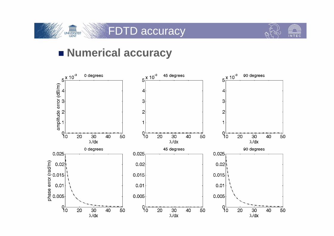
Numerical accuracy Two aspects
Phase error Amplitude error
SIP/SIT p-v FDTD is amplitude-error free At all Courant Numbers
FDTD results in phase errors Phase error decreases with finer spatial
discretisation Phase error vanishes when
– CN=1– Propagation along the diagonal of square cells
FDTD accuracy
2
2
2
2
2
2 )2/(sin)2/(sin)2/(sinarcsin2dz
dzkdy
dykdx
dxkdtc zyx
Numerical accuracy
FDTD accuracy

Including meteorological effects Concept of “background flow”
Most relevant interactions between wind and acoustics in outdoor applications near the ground included
– Convection in uniform flows– Refraction in non-uniform flows– Scattering of sound
No generation of sound The acoustics will not influence the macro-fluid flow
Inhomogeneous atmosphere No additional cost Highest sound speed determines stability criterion
time-domain in OSP
0
1 0pt
0 0v
v v v v20 0c pp
t
0v + v
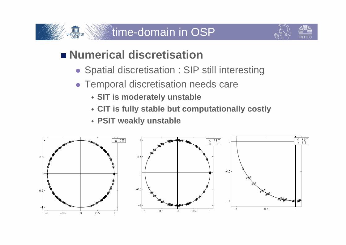
Numerical discretisation Spatial discretisation : SIP still interesting Temporal discretisation needs care
SIT is moderately unstable CIT is fully stable but computationally costly PSIT weakly unstable
time-domain in OSP

Numerical discretisation PSIT scheme
– Second order terms in the flow speed are neglected during discretisation as wind speeds are typically low
– Explicit, efficient scheme still possible– Numerical error
» Small amplitude-errors appear» Phase error is not affected
– see Van Renterghem et al.(Appl. Acoust., 2007)– Can be efficiently implemented
time-domain in OSP
1 2 0.50
l l l-0.5 lnoflowp p dtc dt p 0 v v
1l+0.5 l-0.5 l l lnoflow noflow
0
dt p dt dtρ
0 0v v v v v v

Numerical discretisation
time-domain in OSP

Impedance boundary condition Locally reacting surfaces Models reflection at surfaces only
Including a second medium in the simulation domain Extended reaction (non-local reaction) Models both reflection at surfaces, absorption
inside, and transmission through materials Spatially heterogeneous materials
Finite absorbers

Direct convolution Frequency domain impedance definition:
Each frequency domain signal or function has a time domain analogy
In time domain, we need a convolution which is a computationally costly operation
Impedance boundary cond.
P Z V
*p t Z t v t
1Z t Z
0
t tp t Z t v d Z t v d

Using exp. decaying time-domain functions Efficient direct convolution Recursive approach
Series in j Easy time-domain equivalent Mass-spring-damper system
Pade approximants Examples of application
Attenborough 4-parameter model modified Zwikker and Kosten model
Digital filters Efficient IIR filters Highly flexibility to approach any w-Z curve
Impedance boundary cond.
01
aZj t
1 0 11Z a a a jj
1 0 1
t dv tp t a v t dt a v t a
dt
0
0
ttaZ t e
t
0
0
( )
ni
iim
ii
i
a zZ z
b z

Poro-rigid frame model : Zwikker and Kosten Only the air in between the material matrix is
allowed to vibrate Reasonable when density of the frame and the
stiffness is significantly larger than those of air 3-parameter model
(flow resistivity) (porosity) ks (structure factor)
Including porous medium
0 skpt
0v v
20 0 0cp
t
v
2
0 0
sjZ
kZ

Poro-elastic models : M.A. Biot Coupled movement of frame and air inside the
porous medium included slightly adapted version Parameters
Tortuosity: mt
Porosity: a , f= 1-a
Flow resistivity: Bulk modulus of frame: Kf
Frame density: f
Frame damping coefficient: Rf
Including porous medium
0a aa
a a ffp K Pt
K
v v
2 1aa a a f a
t
aa f
mpt t
v v v v v
f af
ff
a
p pt t
K
v
2 1ff f
tf f a f a a f
a
pt
Rt
m
vv v v v v

Long distance propagation Volume discretisation techniques not well suited
for long-distance propagation Solutions
Moving-frame FDTD– Use of short, broadband pulses– Mainly software challenge
» Allocate and de-allocate memory in an efficient way
– Mainly efficient if propagation is essentially in one-direction
time-domain in OSP
Region a Region b Region c

Long distance propagation Solutions
Hybrid modelling– Many techniques highly efficient in particular
cases– Coupling in an attempt to combine “best of both
worlds”– Coupling in same domain
» BEM-PE– Cross-domain coupling
» Raytracing-analytical formulae (e.g. diffraction)
» BEM-raytracing» FDTD-PE
time-domain in OSP

Long distance propagation Green’s Function Parabolic Equation method
PE-type model : one-way sound propagation, effective sound speed approach, range-dependent impedance and profiles, inclusion of terrain possible (CMM,GTPE,rGFPE), diffraction over thin screen, etc.
Works with vertical array of acoustic pressures Extrapollation towards next array based on Green’s
function Discretisation
– in vertical direction : strong discretisation– in forward direction : stepping at several
wavelengths without loss in accuracy Efficiently uses FFT
time-domain in OSP
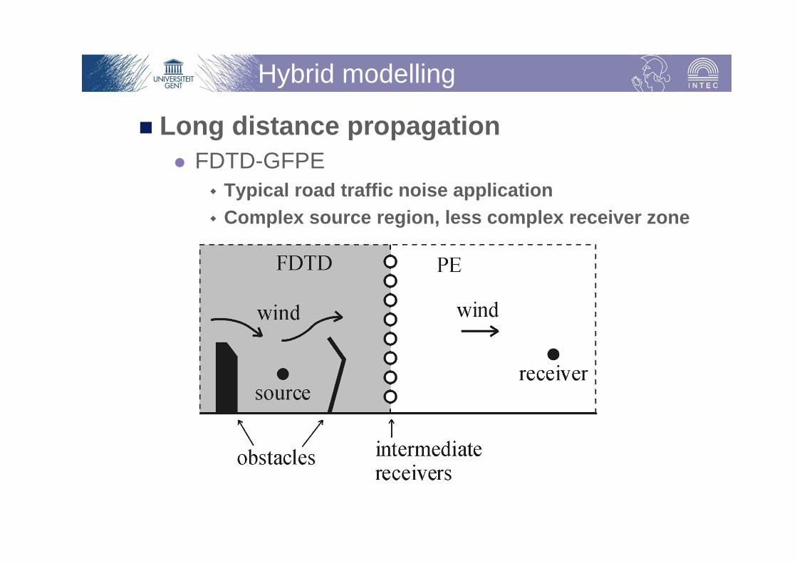
Long distance propagation FDTD-GFPE
Typical road traffic noise application Complex source region, less complex receiver zone
Hybrid modelling
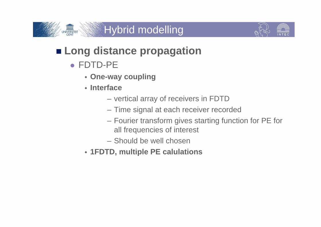
Long distance propagation FDTD-PE
One-way coupling Interface
– vertical array of receivers in FDTD– Time signal at each receiver recorded– Fourier transform gives starting function for PE for
all frequencies of interest– Should be well chosen
1FDTD, multiple PE calulations
Hybrid modelling

Long distance propagation FDTD-PE
Example : evaluation of T-noise barriers in wind
Hybrid modelling

Long distance propagation
Hybrid modelling

Long distance propagation FDTD-PE
Starting fields
Hybrid modelling
0 10 20 30 40 500
0.5
1
1.5
2
height z (m)
mag
nitu
de (
Pa) 100 Hz
0 10 20 30 40 500
0.1
0.2
0.3
0.4
height z (m)
mag
nitu
de (
Pa) 300 Hz
0 10 20 30 40 500
0.1
0.2
0.3
0.4
height z (m)
mag
nitu
de (
Pa) 500 Hz

Hybrid modelling
FDTD 2 mFDTD 4 mFDTD+PE 2 mFDTD+PE 4 m
locationstarting field
locationdownwindnoise barrier

Time-domain modelling in outdoor sound propagation has become mature
Low-order schemes are well suited in outdoor sound propagation when carefully choosing the numerical discretisation scheme
Hybrid modelling for long-distance sound propagation
Current trends in time-domain modelling Parallellisation (by using GPU) Pseudo-spectral time-domain technique (PSTD)
Conclusions
Top Related