1

Efficient Variational Bayesian ApproximationMethod Based on Subspace Optimization

Yuling Zheng, Aurelia Fraysse, Thomas Rodet

Abstract—Variational Bayesian approximations have beenwidely used in fully Bayesian inference for approximating an in-tractable posterior distribution by a separable one. Nevertheless,the classical variational Bayesian approximation (VBA) methodsuffers from slow convergence to the approximate solution whentackling large dimensional problems. To address this problem,we propose in this paper a more efficient VBA method. Actually,variational Bayesian issue can be seen as a functional optimiza-tion problem. The proposed method is based on the adaptation ofsubspace optimization methods in Hilbert spaces to the involvedfunction space, in order to solve this optimization problem inan iterative way. The aim is to determine an optimal directionat each iteration in order to get a more efficient method. Wehighlight the efficiency of our new VBA method and demonstrateits application to image processing by considering an ill-posedlinear inverse problem using a total variation prior. Comparisonswith state of the art variational Bayesian methods through anumerical example show a notable improvement in computationtime.

Index Terms—Variational Bayesian approximation, subspaceoptimization, large dimensional problems, unsupervised ap-proach, total variation

I. INTRODUCTION

EFFICIENT reconstruction approaches for large dimen-sional inverse problems involved in image processing are

the main concerns of this paper. In general, such problemsare ill-posed, which means that the information provided bydata is not sufficient enough to give a good estimation of theunknown object. The resolution of ill-posed inverse problemsgenerally relies on regularizations which consist of introducingadditional information, see [1] for details. One most commonlyused regularization is the Tikhonov one [2]. Nevertheless,Tikhonov regularization leads to an estimator linear withrespect to the data. Therefore, its ability to reconstruct non-linear components, such as location and magnitude of jumpsor higher order discontinuities, see [3] and [4], is limited.

To overcome such limitations, nonlinear regularizationshave been widely used. However, the drawback of those reg-ularizations is the corresponding non-quadratic or even non-convex optimization problems which are generally intricate.To tackle this issue, Geman et al [3], [4] proposed half-quadratic schemes in order to get nonlinear estimates more

Copyright (c) 2013 IEEE. Personal use of this material is permitted.However, permission to use this material for any other purposes must beobtained from the IEEE by sending a request to pubs-permissions@ieee.org.

Y. Zheng and A. Fraysse are with the Laboratory of signals and systems(CNRS-Supelec-University of Paris-Sud). L2S-SUPELEC, 3, Rue Joliot-Curie, 91190 Gif-sur-Yvette, France. (email: zheng,fraysse@lss.supelec.fr)

T. Rodet is with Laboratory of Systems and Applications of Information andEnergy Technologies (Ecole Normale Superieure de Cachan). 61, Avenue duPresident Wilson, 94230 Cachan, France. (email: trodet@satie.ens-cachan.fr)

easily. By introducing auxiliary variables using duality tools,half-quadratic schemes transform the original complicatedcriterion into a half quadratic one where the original variablesappear quadratically and the auxiliary variables are decoupled.This half-quadratic criterion can be efficiently optimized usingclassical optimization algorithms, which lead to the desirednonlinear estimates.

In a statistical framework, the half-quadratic schemes havebeen shown by Champagnat et al. [5] as instances of theEM algorithm with latent variables which provide maximum aposteriori estimates. Nevertheless, for either Tikhonov regular-ization based methods or half-quadratic schemes, only pointestimates could be given. Some useful information such asthe variance of the estimator, which evaluates its precision,could not be directly obtained. However, such informationis accessible if we obtain the posterior distribution of theunknown parameters, which is involved in the Bayesianframework. Moreover, another advantage of the Bayesianframework is that it provides a systematic way to determinehyperparameters, e.g. a Bayesian hierarchical approach canestimate the hyperparameters as well as unknown parametersby introducing hyperpriors, [6] [7]. Such approaches areknown as unsupervised approaches in the literature. In order toexploit these advantages, in this paper we are mainly interestedin unsupervised Bayesian methods. Furthermore, due to thedevelopment of information technologies, we encounter moreand more often large dimensional inverse problems. As aresult, the development of fast approaches has become increas-ingly important. The aim of this paper is therefore to developfast unsupervised Bayesian approaches for large dimensionalinverse problems. Nevertheless, the difficulty met in generalis that one could only acquire a posterior distribution whosepartition function is unknown due to an intractable integral.In such a case, the main challenge is to retrieve the posteriordistribution efficiently.

In this context, two main types of approaches are employed,stochastic approaches and analytic approximations. Stochasticapproaches are based on Markov Chain Monte Carlo (MCMC)techniques [8] which provide an asymptotically exact numeri-cal approximation of the true posterior distribution. The maindrawbacks of such approaches are the high computationalcost and the poor performance for large dimensional prob-lems involving complicated covariance matrices. The use ofsuch approaches for large dimensional problems is thereforelimited.

Concerning analytic methods, MacKay in [9], see also [10]for a survey, proposed the variational Bayesian approximation(VBA) which aims to determine analytic approximations of the

2

true posterior distribution. In this case, the objective is to find asimpler probability density function (pdf), generally separable,which is as close as possible to the true posterior distributionin the sense of minimizing the Kullback-Leibler divergence.This problem can be formulated as an infinite-dimensionaloptimization problem, whose resolution results in an optimalanalytic approximation. However, this approximation does nothave an explicit form except for extremely simple cases. Inpractice, it is generally approached by cyclic iterative methodswhich update at each iteration one component of the separabledistribution while fixing the other ones. Such optimizationprocedure is known to be time consuming in general. Theclassical Bayesian methodology is thus not efficient enoughwhen dealing with very large dimensional problems.

In order to obtain more efficient variational Bayesian ap-proaches, a different method has been recently introducedin [11]. It is based on the adaptation of the exponentiatedgradient algorithm [12] into the space of pdf, which is nolonger a Hilbert space. Instead of approximating an analyticalsolution of the involved functional optimization problem,this method seeks an approximate solution of this problemiteratively thanks to a gradient-type algorithm with explicitupdate equations. The optimization of the components of theseparable approximation can thus be performed in parallel,which leads to a significant acceleration compared to theclassical VBA method.

In order to get a method faster than that of [11], a naturalidea is to consider a new descent direction. In this context,we propose to adapt the subspace optimization methods [13]–[16], into the space of pdf involved in variational Bayesianmethodology. The advantage of subspace optimization is itsgeneralized descent directions where Hilbert structure is notrequired. Moreover, the descent direction can be freely chosenin a subspace of dimension greater than one. This flexibilityallows subspace optimization methods to be generally moreefficient than conjugate gradient methods [17]. Based on thesubspace optimization methods, a faster variational Bayesianoptimization method is proposed in this paper.

As stated above, the objective is to develop fast unsu-pervised Bayesian approaches for large dimensional inverseproblems in image processing. To do this, we consider theapplication of our new variational Bayesian method to suchproblems. In the context of image reconstruction, the totalvariation (TV) regularization has been popular [18], [19] dueto its ability to describe piecewise smooth images. Never-theless, it is difficult to integrate the TV based prior intothe development of unsupervised Bayesian approaches sinceits partition function depends on hyperparameters and it isnot explicitly known. To tackle this problem, Bioucas-Diaset al. [20], [21] proposed a closed form approximation ofthis partition function. Thanks to this approximation, Babacanet al. [22] developed its TV based unsupervised Bayesianapproach using the classical VBA method. In this work,we also take advantage of this approximate TV prior. Withthis prior, we develop our unsupervised approach using theproposed VBA method.

In order to evaluate the proposed approach, we providealso numerical comparisons with [22] which is based on the

classical VBA method, and with another approach employingthe gradient-type variational Bayesian algorithm proposed in[11]. These comparisons are based on an implementation on anexample of linear inverse problems – a linear super-resolutionproblem [23] which aims to reconstruct a high resolutionimage from several low resolution ones representing the samescene. Moreover, to be able to compare the approaches in largedimensional problems, in our reconstruction, we assume thatmotions between the low resolution images and a referenceone could either be estimated in advance or be known throughother sources of information. Such configuration appears in afew applications such as astronomy [24] or medical imaging[25].

The rest of this paper is organized as follows: in SectionII, we develop our proposed variational Bayesian optimizationalgorithm. Next, an application of the proposed algorithm to alinear inverse problem is shown in Section III whereas resultsof numerical experiments on super-resolution problems aregiven in Section IV. Finally, a conclusion is drawn in SectionV.

II. EXPONENTIATED SUBSPACE-BASED VARIATIONALBAYESIAN OPTIMIZATION ALGORITHM

A. Notations

In the following y ∈ RM and w ∈ RJ denote respectivelythe data vector and the unknown parameter vector to beestimated whereas p(w), p(w|y) and q(w) represent theprior distribution, the true posterior law and the approximateposterior distribution, respectively.

B. Statement of the problem

The central idea of variational Bayesian methods is toapproximate the true posterior distribution by a separable one

q(w) =

P∏i=1

qi(wi), (1)

where w = (w1, . . . ,wP ). Here (wi)i=1,...,P denote the Pdisjoint subsets of elements of w with P an integer between1 and J .

The optimal approximation is determined by minimizing ameasure of dissimilarity between the true posterior distributionand the approximate one. A natural choice for the dissimilaritymeasure is the Kullback-Leibler divergence (KL divergence),see [26]:

KL[q‖p(·|y)] =

∫RJq(w) ln

q(w)

p(w|y)dw. (2)

In fact, direct minimization of KL[q‖p(·|y)] is usuallyintractable since it depends on the true posterior p(·|y) whosenormalization constant is difficult to calculate. However, asgiven in [27], the logarithm of the marginal probability of thedata, called also evidence, can be written as

ln p(y) = F(q) +KL[q‖p(·|y)], (3)

where F(q) is the so called negative free energy defined as

F(q) =

∫RJq(w) ln

p(y,w)

q(w)dw. (4)

3

As ln p(y) is a constant with respect to q(w), minimizingthe KL divergence is obviously equivalent to maximizingthe negative free energy. We can see from (4) that for thecomputation of the negative free energy, the joint distributionp(y,w) is involved instead of the true posterior law. And thisjoint distribution can be readily obtained by the product oflikelihood and prior distributions. We use hence the negativefree energy as an alternative to the KL divergence.

Let us define a space Ω which is a space of separable pdf,Ω = q : pdf and q =

∏Pi=1 qi. Our variational Bayesian

problem can be written as

qopt = arg maxq∈Ω

F(q) (5)

Classical variational Bayesian approximation [10] is basedon an analytical solution of (5) (see [10] or [27] for deriva-tions) which is given by q =

∏Pi=1 qi with

qi(wi) = Ki exp(〈ln p(y,w)〉∏

j 6=i qj(wj)

), ∀i = 1, . . . , P.

(6)Here 〈·〉q = Eq[·] and Ki denotes the normalization constant.We can see from (6) that qi depends on the other marginaldistributions qj for j 6= i. As a result, we cannot obtain anexplicit form for q unless in extremely simple cases. Therefore,iterative methods such as the Gauss-Seidel one have to beused to iteratively approach this solution. As a result, classicalvariational Bayesian method is not efficient enough to treathigh dimensional problems.

In this paper, in order to obtain efficient variational Bayesianapproaches, instead of firstly giving an analytical solutionthen iteratively approaching it, we directly propose iterativemethods to approach qopt defined by (5) by solving a concaveoptimization problem in a space of measures which is definedas follows.

Let us firstly define a separable probability measure spaceA =

⊗Pi=1Ai, the Cartesian product of (Ai)i=1,...,P , defined

as follows:

Ai = µi : probability measureand µi(dwi) = qi(wi)dwi with qi a pdf.

The space A can be considered as a subset of the space ofsigned Radon measures M endowed with the norm of totalvariation, which is a Banach space [28]. However, the spaceA is not convex. As we want to solve a convex optimizationproblem, we consider a set A′, the closed convex hull of Ain M. Therefore, as stated in [11], the problem of finding theoptimal approximate distribution defined by (5) can be solvedby considering the following convex optimization problem

µopt = arg maxµ∈A′

F (µ), (7)

where the functional F :M→ R satisfies that ∀µ ∈ A havea density q, F (µ) = F(q). This optimization problem canbe seen as a constrained convex optimization problem in aninfinite dimensional Banach space M.

As M is a Banach space, one can compute the Gateauxdifferential of F onM. Moreover, for the functional F definedabove, one can find a continuous and upper bounded function

∂f :M×RJ → R such that the Gateaux differential of F isgiven by

∀µ, ν ∈M, ∂Fµ(ν) =

∫RJ∂f(µ,w)dν(w). (8)

In the case where µ ∈ A and q is the density of µ, we candefine a functional df by ∀w ∈ RJ ,df(q,w) = ∂f(µ,w). Ifµ ∈ A, then q is separable. In this case, we have df(q,w) =Σidif(qi,wi), in which ∀i = 1, . . . , P , dif(qi,wi) (see [11]for more details of the derivation) is expressed as:

dif(qi,wi) = 〈ln p(y,w)〉∏j 6=i qj(wj)

− ln qi(wi)− 1. (9)

In [11], the gradient descent method in Hilbert spaces hasbeen transposed into the space of probability measures and, asa result, an exponentiated gradient based variational Bayesianapproximation (EGrad-VBA) method whose convergence isproven was proposed to solve the involved functional opti-mization problem (7). For the aim of developing more efficientmethods, we transpose here in the same context the subspaceoptimization method which has been shown to outperformstandard optimization methods, such as gradient or conjugategradient methods, in terms of rate of convergence in finitedimensional Hilbert spaces [17].

C. Subspace optimization method in Hilbert spaces

We give in this section a brief introduction of the sub-space optimization method in Hilbert spaces. The subspaceoptimization method has been proposed by Miele et al. [13]with a subspace spanned by the opposite gradient and theprevious direction. This method is known as Memory Gradient(MG) and can be regarded as a generalization of the conjugategradient method. More recently, a lot of other subspace opti-mization methods based on different subspaces, see [15] and[29] for instances, have been proposed. Generally, subspaceoptimization methods use the following iteration formula:

xk+1 = xk + dk = xk + Dksk, (10)

where xk and xk+1 respectively stands for the estimates at kthand (k + 1)th iterations, Dk = [dk1 , . . . ,d

kI ] gathers I direc-

tions which span the subspace and the vector sk = [sk1 , ..., skI ]T

encloses the step-sizes along each direction. The subspaceoptimization method offers more flexibility in the choice ofdk by taking linear combinations of directions in Dk.

An overview of existing subspace optimization methods[17] shows that Dk usually includes a descent direction (e.g.gradient, Newton, truncated Newton direction) and a shorthistory of previous directions. In this work, we consider onlythe super memory gradient subspace where Dk is given asfollows:

Dk = [−gk,dk−1, . . . ,dk−I+1]. (11)

Here −gk is the opposite gradient and (dk−j)j=1,...,I−1

are the directions of previous iterations. Chouzenoux et al.[17] have addressed a discussion about the dimension ofthe subspace through simulation results on several imagerestoration problems. It is shown that in a Hilbert space,for a super memory gradient subspace (11), taking I = 2i.e. a subspace constructed by the opposite gradient and the

4

previous direction, results in the best performance in termsof computation time. In this case, the super memory gradientsubspace is degraded to the memory gradient one.

D. Proposed subspace-based variational Bayesian approxi-mation method

In this section, we define our iterative method based onthe transposition of the subspace optimization method for theresolution of (7). We use here k ∈ N, set initially to zero, asthe iteration count and assume that µk ∈ A has a density qk.As we stand in the space of probability density measures, thenext iteration should give also a probability density measureabsolutely continuous with respect to µk. The Radon-Nikodymtheorem [30] ensures that this measure should be written as

µk+1(dw) = hk(w)µk(dw), (12)

where hk ∈ L1(µk) is a positive function1. Since µk isa Radon probability measure with a density qk, we canequivalently write

qk+1(w) = hk(w)qk(w), (13)

as updating equation for the approximate density. Furthermore,as we deal with entropy-type functionals, a natural choice forhk would be an exponential form (see [31]). Moreover, thischoice ensures the positivity of pdf along iterations.

Considering the exponential form of hk and the subspaceoptimization principle, we propose

hk(w) = Kk(sk) exp[Dk(w)sk

], (14)

which leads to the updating formula for the measure

µk+1(dw) = Kk(sk) exp[Dk(w)sk

]µk(dw), (15)

and the updating equation for the density

qk+1(w) = Kk(sk) exp[Dk(w)sk

]qk(w). (16)

Here, by abuse of notation, we use Dk(w) to represent theset of directions spanning the subspace in both (15) and(16). Nevertheless, in (15), the directions are in the space ofmeasures whereas in (16), the directions are in the space ofpdf.

The notation Kk(sk) represents the normalization constantexpressed as

Kk(sk) =

[∫RJ

exp[Dk(w)sk

]qk(w)dw

]−1

, (17)

and Dk(w) = [dk1(w), . . . , dkI (w)] is the set of I direc-tions spanning the subspace. We should state that as wedeal with a functional optimization problem, the directions(dkl (w))l=1,...,I , are no longer vectors but functions. Finally,sk = [sk1 , . . . , s

kI ]T denotes the multi-dimensional step-size.

Due to the exponential form, (14) can also be written as:

hk(w) = Kk(sk)[φk1(w)

]sk1 . . . [φkI (w)]skI (18)

where φkl (w) = exp[dkl (w)], for l = 1, . . . , I .

1h ∈ L1(µ) ⇔∫RJ |h(w)|µ(dw) <∞

1) Set of directions spanning the subspace: As discussed inSection II-C, for the super memory gradient subspaces definedin Hilbert spaces (see (11)), the subspace of dimension two,which is known as memory gradient subspace, leads to themost efficient approaches. Moreover, a subspace of dimensiontwo would result in less computation complexity than higherorder subspaces. As a result, we consider in this work thetransposition of the memory gradient subspace into the spaceof probability measures. In this case, I = 2. The transpositionleads to a Dk(w) consisting of one term related to the Gateauxdifferential of F and the other term corresponding to theprevious direction.

When µ has a density q, the structure of our MemoryGradient (MG) subspace in the space of pdf is given by

DkMG(w) = [df(qk,w), dk−1(w)], (19)

where ∀qk ∈ Ω, df(qk, ·) = Σidif(qki ,wi) with dif(qki ,wi)is given by (9) and dk−1 stands for the direction of the previousiteration, which is given by

dk−1(w) = ln

(qk(w)

Kk−1(sk−1)qk−1(w)

). (20)

Our proposed variational Bayesian approximation methodbased on this subspace is called exponentiated memory gradi-ent subspace-based variational Bayesian approximation in therest of this paper and is summarized in Algorithm 1.

Algorithm 1 Exponentiated Memory Gradient subspace-basedVariational Bayesian Approximation (EMG-VBA)

1) Initialize(q0 ∈ Ω)2) repeat

a. determine subspace DkMG(w) using (9), (19) and

(20)b. determine step-sizes sk

c. compute

qk+1(w) =Kk(sk) exp[DkMG(w)sk

]qk(w)

=Kk(sk)qk(w)

× exp[sk1df(qk,w) + sk2d

k−1(w)]

(21)

until convergence

E. The approximate step-size

Let us firstly define a function gk

gk : R2 → R gk(s) = F(Kk(s) exp

[DkMG(w)s

]qk(w)

),

(22)then the optimal step-size is given by

(sopt)k = arg maxs∈R2

gk(s). (23)

Generally, it is too expensive to get the optimal step-size.Therefore, in practice most iterative approaches take sub-optimal ones considering the trade-off between computationalcost and difference from the optimal step-size. To make a such

5

trade-off, in this work, we adopt a backtracking line search likestrategy [32] as described in the following.

Firstly, an initial step-size calculated in the following wayis proposed. We take the second order Taylor expansion ofgk(s) at origin as local approximation,

gk(s) = gk(0) +

(∂gk

∂s

∣∣∣∣s=0

)Ts +

1

2sT(∂2gk

∂s∂sT

∣∣∣∣s=0

)s,

(24)where ∂gk

∂s

∣∣s=0

denotes the gradient vector whereas ∂2gk

∂s∂sT

∣∣s=0

is the Hessian matrix of the function gk at s = 0. When s1

and s2 are small, gk(s) is a close approximation of gk(s).Our initial step-size is then computed by maximizing

gk(s) which is quadratic. Assuming that the Hessian matrix∂2gk

∂s∂sT

∣∣s=0

is invertible, this initial step is given by

sk = −(∂2gk

∂s∂sT

∣∣∣∣s=0

)−1∂gk

∂s

∣∣∣∣s=0

. (25)

Secondly, we determine our trade-off sub-optimal step-size(ssubopt)k from sk. If sk obtained by (25) leads to the increaseof the criterion as we expect, i.e. gk(sk) > gk(0), then wetake directly sk as our sub-optimal step-size, (ssubopt)k = sk.Conversely, if this step-size is too large, which leads to thedecrease of the criterion, we divide it iteratively by 2 until weget a step-size (ssubopt)k = 2−tsk (t being the number of timesof divisions) satisfying gk((ssubopt)k) > gk(0). However, inpractice, we find that the proposition given by (25) ensuresthe increase of the criterion in nearly all the iterations.

III. APPLICATION TO A LINEAR INVERSE PROBLEM WITHA TOTAL VARIATION PRIOR

We show in this section an application of the proposedEMG-VBA to ill-posed inverse problems in image processing.Variational Bayesian approaches are widely used to tackleinverse problems where complicated posterior distributions areinvolved. In the following, we firstly present such a problemwhich adopts a Total Variation (TV) prior. Then we developan unsupervised Bayesian approach with the proposed EMG-VBA.

A. Direct model

We consider here a classical linear direct model:

y = Ax + n, (26)

where y ∈ RM and x ∈ RN denote respectively dataand unknown parameters to be estimated arranged in columnlexicographic ordering. The linear operator A ∈ RM×N isassumed to be known and n is an additive white noise,assumed to be i.i.d. Gaussian, n ∼ N (0, γ−1

n I), with γn as aprecision parameter, i.e. the inverse of the noise variance. Thedirect model (26) and the hypothesis of i.i.d. Gaussian noiseallow an easy derivation of the likelihood function:

p(y|x, γn) ∝ γM/2n exp

[−γn‖y −Ax‖2

2

]. (27)

B. Image model

In this work, we consider an image model, more precisely aprior distribution of the unknown x, satisfying two main prop-erties. Firstly, it is able to describe the piecewise smoothnessproperty of images. In the literature, total variation has beenlargely used in various imaging problems including denoising[18], blind deconvolution [33], inpainting [34] and super-resolution [22]. Secondly, we should have some knowledgeof its partition function in order to develop unsupervisedapproaches which sidestep the difficulty of tuning hyperparam-eters. Both demands described above lead us to the work ofBabacan et al. [22], where an unsupervised Bayesian approachusing the total variation (TV) prior was developed. The TVprior is given by

p(x|γp) =1

ZTV (γp)exp [−γpTV (x)] , (28)

where ZTV (γp) is the partition function and

TV (x) =

N∑i=1

√(Dhx)2

i + (Dvx)2i . (29)

Here Dh and Dv represent first-order finite difference matricesin horizontal and vertical directions, respectively.

The major difficulty is that there is no closed form ex-pression for the partition function ZTV (γp). To overcomethis difficulty, Bioucas-Dias et al. [20], [21] proposed anapproximate partition function

ZTV (γp) ' Cγ−θNp , (30)

where C is a constant and θ is a parameter which has tobe adjusted in practice to get better results. This analyticapproximation results in

p(x|γp) ' p(x|γp) = CγθNp exp [−γpTV (x)] , (31)

where C = C−1. Babacan et al. [22] adopted this approximateTV prior with θ = 1/2. In such a case, ZTV (γp) is approxi-mated by Cγ−N/2p which corresponds to the partition functionof a multivariate normal distribution of a N-dimensional ran-dom vector. However, a TV prior is not similar to a Gaussianone. Therefore, this approximation is not close enough. As aresult, in this paper, we keep the parameter θ and adjust it inpractice.

C. Hyperpriors

The hyperparameters γn and γp play an important role inthe performance of algorithms. In practice, choosing correcthyperparameters is far from a trivial task. Therefore, weprefer to automatically determine their values. This is doneby introducing hyperpriors for the hyperparameters. In orderto obtain numerically implementable approaches, conjugatehyperpriors are employed. For γn and γp, we use Gammadistributions,

p(γn) = G(γn|an, bn) (32)

p(γp) = G(γp|ap, bp) (33)

6

where for a > 0 and b > 0

G(z|a, b) =ba

Γ(a)za−1 exp (−bz) (34)

As we do not have any prior information about γn and γp,in practice, we consider an = 0, bn = 0 and ap = 0, bp = 0,which lead to non-informative Jeffreys’ priors.

Consequently, we obtain a joint distribution as follows

p(y,x, γn, γp) ∝ γM/2n exp

[−γn‖y −Ax‖2

2

]× γθNp exp

[−γp

N∑i=1

√(Dhx)2

i + (Dvx)2i

]γ−1n γ−1

p

(35)

where ∝ means “is approximately proportional to”. The pos-terior distribution p(x, γn, γp|y) is not known explicitly sincethe normalization constant is not calculable. In order to pro-ceed the statistic inference of the unknown variables, we resortto the variational Bayesian approximation methods which aimat getting the best separable analytical approximation. In thecontext of variational Bayesian methods, in order to get numer-ically implementable approaches, conjugate priors are neededto ensure that each posterior distribution belongs to a givenfamily. Consequently, the optimization of the approximatedistribution can be reduced to a numerical approximation ofits parameters. Nevertheless, the TV prior introduced aboveis not conjugate with the likelihood (see (27)) which is aGaussian distribution. To tackle this problem, Minorization-Maximization (MM) techniques [35] are employed here to geta conjugate variant, as done by Babacan et al. in [22].

D. Application of variational Bayesian approximation meth-ods

Let Θ denote the set of all unknown parameters: Θ =x, γn, γp, the objective of variational Bayesian approxi-mations is to give a tractable approximation qΘ of the trueposterior distribution p(·|y). As the TV prior is not conjugatewith the likelihood, it is difficult to carry out the maximizationof the negative free energy with respect to qΘ. This diffi-culty has been solved by adopting Minorization-Maximization(MM) techniques [35], in which maximizing the negative freeenergy is substituted by maximizing a tractable lower bound.To get such a lower bound of the negative free energy, a lowerbound of the approximate TV prior is firstly constructed byintroducing positive auxiliary variables λ = [λ1, . . . , λN ], see[22] for details,

p(x|γp) ≥M(x, γp|λ) = CγθNp

× exp

[−γp

N∑i=1

(Dhx)2i + (Dvx)2

i + λi

2√λi

]. (36)

From (36), we can see that the lower bound of the TV prior,M(x, γp|λ), is proportional to a Gaussian distribution and istherefore conjugate to the likelihood. Combining (4) and (36),

a lower bound of the negative free energy can be derived as

F(qΘ) ≥FL(qΘ,λ)

=

∫qΘ(Θ) ln

(L(Θ,y|λ)

qΘ(Θ)

)dΘ, (37)

where

L(Θ,y|λ) = p(y|x, γn)M(x, γp|λ)p(γn)p(γp) (38)

is a lower bound of the joint distribution.Hence the resolution of the problem (5) is performed by

alternating the two following steps: maximizing the lowerbound FL with respect to the pdf qΘ and updating theauxiliary variable λ in order to maximize FL. Assuming that

qΘ(Θ) = qx(x)qγn(γn)qγp(γp)

=∏i

qi(xi)qγn(γn)qγp(γp), (39)

we carry out an alternate optimization of FL with respectto qx, qγn , qγp and λ. Altogether, we perform the followingalternate iterative scheme2:

qk+1x = arg max

qx

FL(qxq

kγnq

kγp ,λ

k), (40)

λk+1 = arg maxλ∈RN

FL(qk+1x qkγnq

kγp ,λ

)(41)

qk+1γn = arg max

qγn

FL(qk+1x qγnq

kγp ,λ

k+1), (42)

qk+1γp = arg max

qγp

FL(qk+1x qk+1

γn qγp ,λk+1)

(43)

The functional optimizations with respect to qx, qγn andqγp (given by (40), (42) and (43), respectively) are solvedby variational Bayesian approximation methods. Since theconditional posterior p(γn, γp|x,y) is separable, it could beapproximated efficiently thanks to the classical VBA. In fact,the proposed EMG-VBA is only adopted to approximate theposterior distribution of x where it improves the rate ofconvergence. And this is one of the major differences with theapproach proposed in [22] which employs the classical VBAto determine qk+1

x , as will be explained in Section III-E1. Asregards the optimization of the auxiliary variable λ (given by(41)), it involves a classical optimization in a Hilbert space.

Due to the use of MM techniques, we manage to get aprior for x conjugate with the likelihood. Moreover, conjugateGamma priors are chosen for hyperparameters γn and γp.Therefore, the optimal approximations (qi)i=1,...,N belong toa Gaussian family whereas the optimal approximate posteriordistributions of hyperparameters qγn and qγp belong to aGamma one.

qkx(x) =∏i

N (xi|(mk)i, (σ2k)i), (44)

qkγn(γn) = G(γn|akγn , bkγn), (45)

qkγp(γp) = G(γp|akγp , bkγp), (46)

where mk and σ2k are vectors containing means and variances

of (qi)i=1,...,N , respectively. Therefore, the optimization of

2The auxiliary variable λ is chosen to be updated before qγn and qγp inorder to get a simpler iteration formula for qγp , see [22].

7

approximate distributions can be performed by iterativelyupdating their parameters.

1) Optimization of qx using the proposed EMG-VBA:Regarding the MG subspace, since we maximize here thelower bound FL of the negative free energy, its first directiondf(qkx,x) should be adapted for this new objective function.We can see from (37) that FL differ from F in replacingthe joint distribution by its lower bound. Therefore, the newdirection, denoted by dfL(qkx,x) can be easily obtained bytaking this difference into consideration. Since qx is assumedto be separable, we have dfL(qkx,x) =

∑i dif

L(qki , xi) inwhich ∀i = 1, . . . , N ,

difL(qkx, xi) =

⟨lnL(Θ,y|λk)

⟩∏j 6=i q

kj (xj)

− ln qki (xi)− 1.

(47)According to (13), (14), (19), (20) and (47), we get a

distribution of x depending on the step-size s:

qsx(x) = Kk(s)qkx(x) exp(s1dfL(qkx,x) + s2dk−1(x))

= Kk(s)qkx(x)∏i

[exp[⟨

lnL(Θ,y|λk)⟩(∏j 6=i q

kj )qkγnqkγp

]qki (xi)

]s1×[qki (xi)

qk−1i (xi)

]s2= Kk(s)qkx(x)

∏i

[qri (xi)

qki (xi)

]s1[ qki (xi)

qk−1i (xi)

]s2, (48)

where qri (xi) = exp[⟨

lnL(Θ,y|λk)⟩(∏j 6=i q

kj )qkγnqkγp

]is an

intermediate function which can be expressed as

qri (xi) = exp

[⟨lnL(Θ,y|λk)

⟩(∏j 6=i q

kj )qkγnq

kγp

]∝ exp

[− 〈γn〉

k

2

(x2i diag

(ATA

)i− 2xi

(ATy

)i

+ 2xi(ATAmk

)i− 2xidiag

(ATA

)i(mk)i

)− 〈γp〉

k

2

(x2i diag

(DThΛkDh + DT

v ΛkDv

)i

+ 2xi(DThΛkDhmk + DT

v ΛkDvmk

)i

− 2xidiag(DThΛkDh + DT

v ΛkDv

)i(mk)i

)](49)

where 〈z〉k = Eqkz (z), Λk = Diag(

1√λki

)is a diagonal ma-

trix with(

1√λki

)i=1,...,N

as its elements. Moreover, diag (M)

is a vector whose entries are the diagonal elements of matrixM. The details for the derivation of qri (xi) can be found inAppendix A.

From (49), we can see that (qri )i=1,...,N corresponds, upto the normalization constant, to the density of a Gaussiandistribution with mean (mr)i and variance (σ2

r)i expressed

explicitly as follows:

(σ2r)i =

[〈γn〉kdiag

(ATA

)i

+ 〈γp〉kdiag(DThΛkDh + DT

v ΛkDv

)i

]−1, (50)

(mr)i =(σ2r)i

[〈γn〉k

(ATy −ATAmk + diag(ATA) mk

)i

− 〈γp〉k(DThΛkDhmk + DT

v ΛkDvmk

)i

+ 〈γp〉kdiag(DThΛkDh + DT

v ΛkDv

)i(mk)i

],

(51)

where denotes the Hadamard product between two vectors.Based on the above results for qri , using (48), we can

derive the expression of qsx(x) =∏i q

si (xi) where each

component qsi (xi) is a Gaussian distribution with mean (ms)iand variance (σ2

s )i satisfying:

σ2s =

[1

σ2k

+ s1

(1

σ2r

− 1

σ2k

)+ s2

(1

σ2k

− 1

σ2k−1

)]−1

,

(52)

ms = σ2s

[mk

σ2k

+ s1

(mr

σ2r

− mk

σ2k

)+ s2

(mk

σ2k

− mk−1

σ2k−1

)].

(53)

In above equations, we omit all the indication of vectorcomponent (·)i for the sake of clarity. From (52), we can seethat σ2

s is equal to the inverse of a linear combination of threeterms where the first term is the present inverse variance, thesecond term comes from the gradient and the third term iscaused by the memory of the previous direction. From (53),we can see that ms has the same structure. As stated earlier,the EGrad-VBA can be identified as the proposed EMG-VBAwith s2 set to zero which leads to the elimination of thethird term in (52) and (53). Because of the extra term (thethird term) compared to EGrad-VBA, EMG-VBA can obtaina closer approximation than EGrad-VBA in one iteration.

The previous distribution is still a function of the step size.A sub-optimal step-size defined by (25) in Section II-E is thenadopted. As a result, σ2

k+1 = σ2ssubopt and mk+1 = mssubopt .

2) Optimization of λ in Hilbert spaces: The elements ofauxiliary vector λ are calculated by maximizing the lowerbound FL with respect to (λi)i=1,...,N . Since FL is concaveand differentiable with respect to (λi)i=1,...,N , its maximumis achieved at the critical point which is given by

λk+1i =Eqk+1

x

[(Dhx)2

i + (Dvx)2i

]=Eqk+1

x

[xT (Dh)Ti (Dh)ix + xT (Dv)

Ti (Dv)ix

]=(Dhmk+1)2

i + (Dvmk+1)2i

+ trace[(Dh)Ti (Dh)iΣk+1)

]+ trace

[(Dv)

Ti (Dv)iΣk+1)

], (54)

where (Dh)i and (Dv)i represent the ith row of Dh andDv , respectively. And Σk+1 = Diag

(σ2k+1

)is the covariance

matrix which is diagonal under the separability hypothesis.3) Optimization of qγn and qγp using classical VBA: These

two distributions are computed using (6). More details ofthe calculus can be found in [22]. The means of Gamma

8

distributions are used as the estimates of hyperparameterswhich are

〈γn〉k+1 =M

Eqk+1x

[‖y −Ax‖2], (55)

〈γp〉k+1 =θN∑N

i=1

√λk+1i

. (56)

Altogether, the proposed algorithm for inverse problemusing TV prior is summed up in Algorithm 2.

Algorithm 2 Proposed unsupervised variational Bayesianapproach

1) Initialize parameters of (q0i )i=1,...,N , q0

γn , q0γp and λ

2) Update means and variances of qk+1i for i = 1, . . . , N

a. Compute parameters of intermediary functions qriusing (50), (51)

b. Determine the sub-optimal step-sizes(ssubopt1 , ssubopt2 ) (see Section II-E)

c. Update means and variances of qk+1i using (52),

(53)3) Update auxiliary vector λk+1 using (54)4) Determine the parameters of qk+1

γn and compute its meanby (55)

5) Determine the parameters of qk+1γp and compute its mean

by (56)6) Go back to 2) until a convergence criterion is satisfied.

E. State of the art approaches

1) A classical VBA based approach [22]: The linear inverseproblem with TV image prior treated above has also beentreated recently by Babacan et al. in [22] in the context of aclassical super-resolution problem.

Two major differences exist between the approach proposedin [22] and our approach presented in Section III-D. The firstone is that Babacan et al. used the classical VBA for theoptimization of qx whereas we adopt the proposed EMG-VBA. The second difference is that we assume that qx is fullyseparable whereas Babacan et al. supposed that it is not, moreprecisely

qΘ(Θ) = qx(x)qγn(γn)qγp(γp). (57)

Due to the non-separability assumption, classical VBA basedon (6) yields a multivariate Gaussian distribution for qkx.Updating the distribution is also equivalent to updating itsparameters, i.e. mean mk and covariance matrix Σk. Theupdating equations for these two parameters are given by

mk+1 =Σk+1

[〈γn〉kATy

], (58)

(Σk+1)−1 =〈γn〉kATA

+ 〈γp〉k(DThΛkDh + DT

v ΛkDv

). (59)

However, as we can see from (58), mk+1 depends on thecovariance matrix Σk+1 but the computation of Σk+1 needsthe inversion of the matrix given by (59) which is very costly

or even impossible in large dimensional cases. To bypass thematrix inversion, Babacan et al. have adopted the conjugategradient method to iteratively approximate mk+1, which canbe inefficient in large dimensional cases. For the optimizationof the auxiliary variable λ and the hyperparameters γn, γp, thesame updating equations as (54), (55) and (56) are obtained.In (54) where the covariance matrix Σk+1 is needed, it isapproximated by a diagonal matrix whose diagonal entries areequal to the inverse of the diagonal elements of (Σk+1)−1.Generally, this approximation is not a precise one.

2) EGrad-VBA [11] based approach: We present in thissection another approach for comparison which treats thesame inverse problem. The only major difference between thisapproach and the proposed one is that the EGrad-VBA usingapproximate optimal step-sizes defined in a same way as (25)is adopted for the optimization of qx. For EGrad-VBA, itsupdating formula is given by

qk+1grad (w) = Kk(sk1) exp

[sk1df(qk,w)

]qk(w), (60)

Comparing (60) and (21), we notice that the EGrad-VBA canbe seen as a special case of our EMG-VBA algorithm withthe second step-size s2 set to zero. As a result, there is noneed to show the details of the application of EGrad-VBA intoour inverse problem. The updating equations of the mean andvariance of qx could be easily obtained by considering s2 =0 in (52) and (53). The updating equations for the auxiliaryvariable λ and the hyperparameters γn, γp are still the sameas (54), (55) and (56).

IV. EXPERIMENTAL EVALUATION

The performance of the proposed approach (Algorithm 2)is evaluated through an application on a super-resolution (SR)problem. A SR problem is covered by the linear direct model(26) with a system matrix A gathering the warping, blurringand down-sampling operators. In fact, the main concern ofthis section is the evaluation of the time efficiency of the newvariational Bayesian algorithm EMG-VBA by comparisonswith the existing variational Bayesian approximation tech-niques, classical VBA and EGrad-VBA [11] for the estimationof images. Therefore, we treat here a non-classical super-resolution problem where, for the sake of simplicity, thesystem matrix A is assumed to be known, i.e. no motionparameters are estimated. Meanwhile, this assumption wouldreduce the implementation limitation of a state of the artapproach based on classical VBA [22] to large dimensionalproblems. This state of the art approach based on the classicalVBA and another one using the EGrad-VBA have been brieflyintroduced in Section III-E1 and Section III-E2, respectively.In the following, we show the comparisons of the proposedapproach with these two state of the art ones.

In the following, the approach of Babacan et al. [22] isnamed VBA-SR whereas the EGrad-VBA based approach isreferred to as EGrad-SR. The objective of SR is to constructa High-Resolution (HR) image from several degraded Low-Resolution (LR) images representing the same scene, i.e.data. In our experiments, four groups of LR images aregenerated from four standard images, Testpat and Cameraman

9

of dimension 256 × 256 and Lena, Jetplane of dimension512×512. During the generation of LR images, a 3×3 uniformblur kernel and a decimation factor of 4 in both horizontaland vertical directions are used. Moreover, we add i.i.d. whiteGaussian noises at SNR levels of 5 dB, 15 dB, 25 dB, 35 dBand 45 dB. However, for the sake of simplicity, we treat aproblem where LR images are without rotation and motionsare supposed to be known. During the reconstruction, we taketwelve LR images as data and assume that the convolutionkernel, decimation factor and shifting of LR images are allknown. Since the decimation factor of 4 is used, the size of aLR image is 1

16 of that of the HR image. As a result, the sizeof twelve LR images is smaller than that of the objective HRimage.

In fact, all the considered approaches are based on a sameBayesian model and tackle the same optimization problem.Therefore, in general, these approaches lead to similar re-construction results. The main concern of this comparison istheir rate of convergence. To have a fair comparison, we takethe same initializations for all the approaches: m0 = ATyas the mean and 100 as the variance of HR image pixels,the initializations of the auxiliary variables and the hyperpa-rameters are computed from m0 using (54), (55) and (56).Moreover, the parameter θ involved in the partition functionof the image prior needs to be adjusted. A set of experimentscarried out with different images show that the best results areachieved with θ = 1.1. As a result, we set θ = 1.1 for all ourexperiments.

As convergence criterion of the VBA-SR we use ‖mk −mk−1‖/‖mk−1‖ < 10−5, where mk and mk−1 representsthe estimate of the HR image at kth and (k − 1)th iteration,respectively. And for EGrad-SR and our approach, they stopwhen they achieve a HR image of a PSNR value very close(difference within 1‰) to that obtained by VBA-SR.

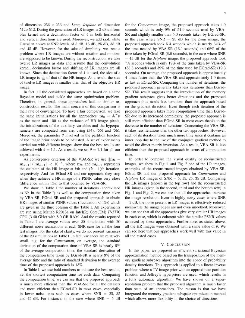
We show in Table I the number of iterations (abbreviatedas Nb in the Table I) as well as the computation time takenby VBA-SR, EGrad-SR and the proposed approach to obtainHR images of similar PSNR values (fluctuation < 1‰) whichare given in the third column of the Table I. All experimentsare run using Matlab R2013a on Intel(R) Core(TM) i7-3770CPU (3.40 GHz) with 8.0 GB RAM. And the results reportedin Table I are average values over 20 simulations with 20different noise realizations at each SNR case for all the fourtest images. For the sake of clarity, we do not present variancesof the 20 simulations in Table I. In fact, variances are relativelysmall, e.g. for the Cameraman, on average, the standardderivation of the computation time of VBA-SR is nearly 6%of the average computation time, the standard derivation ofthe computation time taken by EGrad-SR is nearly 9% of theaverage time and the ratio of standard derivation to the averagetime of the proposed approach is 13%.

In Table I, we use bold numbers to indicate the best results,i.e. the shortest computation time for each data. Comparingthe computation time, we can see that the proposed approachis much more efficient than the VBA-SR for all the datasetsand more efficient than EGrad-SR in most cases, especiallyin lower noise ones such as cases where SNR = 25, 35and 45 dB. For instance, in the case where SNR = 5 dB

for the Cameraman image, the proposed approach takes 4.9seconds which is only 9% of 51.9 seconds used by VBA-SR and slightly smaller than 5.0 seconds taken by EGrad-SR,in the case where SNR = 25 dB for the Lena image, theproposed approach took 5.4 seconds which is nearly 34% ofthe time needed by VBA-SR (16.1 seconds) and 68% of thetime taken by EGrad-SR (8.0 seconds), in the case where SNR= 45 dB for the Jetplane image, the proposed approach took7.5 seconds which is only 19% of the time taken by VBA-SR(38.8 seconds) and 39% of the time used by EGrad-SR (19.3seconds). On average, the proposed approach is approximately4 times faster than the VBA-SR and approximately 1.9 timesas fast as EGrad-SR. Comparing the number of iterations, theproposed approach generally takes less iterations than EGrad-SR. This result suggests that the introduction of the memorygradient subspace gives better directions and the proposedapproach thus needs less iterations than the approach basedon the gradient direction. Even though each iteration of theproposed approach takes more computation time than EGrad-SR due to its increased complexity, the proposed approach isstill more efficient than EGrad-SR in most cases thanks to thedecrease in the number of iterations. Concerning the VBA-SR,it takes less iterations than the other two approaches. However,each of its iteration takes much more time since it contains aninner loop due to the use of the conjugate gradient method toavoid the direct matrix inversion. As a result, VBA-SR is lessefficient than the proposed approach in terms of computationtime.

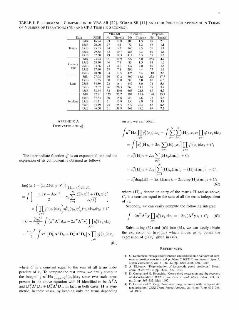
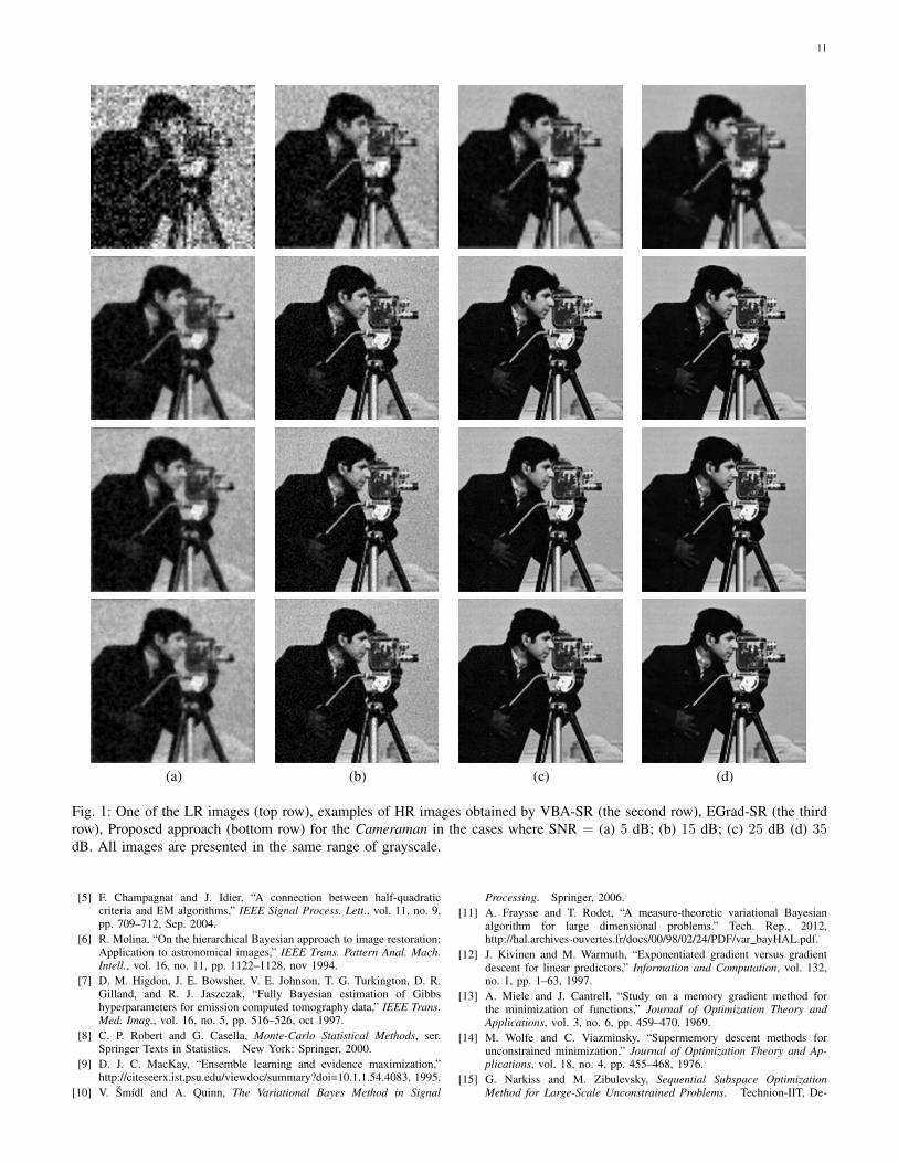
In order to compare the visual quality of reconstructedimages, we show in Fig. 1 and Fig. 2 one of the LR images,examples of the reconstructed images obtained by VBA-SR,EGrad-SR and our proposed approach for Cameraman andJetplane LR images of SNR = 5, 15, 25, 35 dB. Comparingthe LR images (shown in the top row) and the reconstructedHR images (given in the second, third and the bottom row) inFig. 1 and Fig. 2, we can see that all the approaches increasethe image resolution. Even in highly noisy cases where SNR= 5 dB, the noise present in LR images is effectively reducedmeanwhile the image edges are not over-smoothed. Moreover,we can see that all the approaches give very similar HR imagesin each case, which is coherent with the similar PSNR valuesachieved by these approaches. Furthermore, as stated above,all the HR images were obtained with a same value of θ. Wecan see here that our approaches work well with this value inall the tested cases.

V. CONCLUSION

In this paper, we proposed an efficient variational Bayesianapproximation method based on the transposition of the mem-ory gradient subspace algorithm into the space of probabilitydensity functions. This approach is applied to a linear inverseproblem where a TV image prior with an approximate partitionfunction and Jeffrey’s hyperpriors are used, which results ina fully automatic algorithm. We have shown on a super-resolution problem that the proposed algorithm is much fasterthan state of art approaches. The reason is that we haveintegrated the memory gradient subspace optimization methodwhich allows more flexibility in the choice of directions.

10

TABLE I: PERFORMANCE COMPARISON OF VBA-SR [22], EGRAD-SR [11] AND OUR PROPOSED APPROACH IN TERMSOF NUMBER OF ITERATIONS (Nb) AND CPU TIME (IN SECONDS).

VBA-SR EGrad-SR ProposedData PSNR Nb Time(s) Nb Time(s) Nb Time(s)

Testpat

5dB 16.84 83 12.8 100 1.5 99 2.015dB 20.96 27 4.1 72 1.2 58 1.125dB 25.55 24 5.3 165 2.5 55 1.235dB 29.85 33 10.7 283 4.3 69 1.445dB 32.60 49 19.3 412 6.3 78 1.6

Camera-man

5dB 23.24 181 51.9 327 5.0 254 4.915dB 28.70 46 7.1 85 1.3 81 1.625dB 33.36 23 4.6 137 2.0 69 1.535dB 37.40 28 7.8 290 4.4 75 1.645dB 40.50 34 13.5 425 6.4 110 2.3

Lena

5dB 27.08 96 87.2 300 16.1 232 17.715dB 31.35 30 17.0 92 5.0 85 6.525dB 34.59 22 16.1 147 8.0 71 5.435dB 37.07 26 26.3 260 14.1 77 5.945dB 38.44 32 40.0 405 21.8 87 6.7

Jetplane

5dB 32.91 123 72.7 197 10.6 180 13.715dB 37.33 30 15.6 84 4.5 74 5.625dB 41.21 21 15.9 150 8.0 71 5.435dB 44.49 25 25.5 379 20.1 85 6.545dB 46.60 31 38.8 362 19.3 99 7.5

APPENDIX ADERIVATION OF qri

The intermediate function qri is an exponential one and theexpression of its component is obtained as follows:

lnqri (xi) =⟨lnL(Θ,y|λk)

⟩(∏j 6=i q

kj )qkγnqkγp

=

∫ [− γn‖y −Ax‖2

2− γp

N∑i=1

(Dhx)2i + (Dvx)2

i

2√λki

]×(∏j 6=i

qkj (xj)dxj

)qkγn(γn)qkγp(γp)dγndγp + C

=C − 〈γn〉k

2

∫ (xTATAx− 2xTATy

)∏j 6=i

qkj (xj)dxj

− 〈γp〉k

2

∫xT[DThΛkDh + DT

v ΛkDv

]x∏j 6=i

qkj (xj)dxj ,

(61)

where C is a constant equal to the sum of all terms inde-pendent of xi. To compute the rest terms, we firstly computethe integral

∫xTHx

∏j 6=i q

kj (xj)dxj since two such terms

present in the above equation with H identified to be ATAand DT

hΛkDh + DTv ΛkDv . In fact, in both cases, H is sym-

metric. In these cases, by keeping only the terms depending

on xi, we can obtain∫xTHx

∏j 6=i

qkj (xj)dxj =

∫ N∑p=1

N∑l=1

(H)plxpxl∏j 6=i

qkj (xj)dxj

=

∫ [x2i (H)ii + 2xi

∑p 6=i

(H)ipxp

]∏j 6=i

qkj (xj)dxj + C1

= x2i (H)ii + 2xi

∑p 6=i

(H)ip(mk)p + C1

= x2i (H)ii + 2xi

[ N∑p=1

(H)ip(mk)p − (H)ii(mk)i

]+ C1

= x2i diag(H)i + 2xi(Hmk)i − 2xidiag(H)i(mk)i + C1

(62)

where (H)ij denote an entry of the matrix H and as above,C1 is a constant equal to the sum of all the terms independentof xi.

Secondly, we can easily compute the following integral:∫−2xTATy

∏j 6=i

qkj (xj)dxj = −2xi(ATy)i + C2 (63)

Substituting (62) and (63) into (61), we can easily obtainthe expression of ln qri (xi) which allows us to obtain theexpression of qri (xi) given in (49).

REFERENCES

[1] G. Demoment, “Image reconstruction and restoration: Overview of com-mon estimation structure and problems,” IEEE Trans. Acoust. Speech,Signal Processing, vol. 37, no. 12, pp. 2024–2036, Dec. 1989.

[2] A. Tikhonov, “Regularization of incorrectly posed problems,” Soviet.Math. Dokl., vol. 4, pp. 1624–1627, 1963.

[3] D. Geman and G. Reynolds, “Constrained restoration and the recoveryof discontinuities,” IEEE Trans. Pattern Anal. Mach. Intell., vol. 14,no. 3, pp. 367–383, Mar. 1992.

[4] D. Geman and C. Yang, “Nonlinear image recovery with half-quadraticregularization,” IEEE Trans. Image Process., vol. 4, no. 7, pp. 932–946,Jul. 1995.

11

(a) (b) (c) (d)

Fig. 1: One of the LR images (top row), examples of HR images obtained by VBA-SR (the second row), EGrad-SR (the thirdrow), Proposed approach (bottom row) for the Cameraman in the cases where SNR = (a) 5 dB; (b) 15 dB; (c) 25 dB (d) 35dB. All images are presented in the same range of grayscale.

[5] F. Champagnat and J. Idier, “A connection between half-quadraticcriteria and EM algorithms,” IEEE Signal Process. Lett., vol. 11, no. 9,pp. 709–712, Sep. 2004.

[6] R. Molina, “On the hierarchical Bayesian approach to image restoration:Application to astronomical images,” IEEE Trans. Pattern Anal. Mach.Intell., vol. 16, no. 11, pp. 1122–1128, nov 1994.

[7] D. M. Higdon, J. E. Bowsher, V. E. Johnson, T. G. Turkington, D. R.Gilland, and R. J. Jaszczak, “Fully Bayesian estimation of Gibbshyperparameters for emission computed tomography data,” IEEE Trans.Med. Imag., vol. 16, no. 5, pp. 516–526, oct 1997.

[8] C. P. Robert and G. Casella, Monte-Carlo Statistical Methods, ser.Springer Texts in Statistics. New York: Springer, 2000.

[9] D. J. C. MacKay, “Ensemble learning and evidence maximization,”http://citeseerx.ist.psu.edu/viewdoc/summary?doi=10.1.1.54.4083, 1995.

[10] V. Smıdl and A. Quinn, The Variational Bayes Method in Signal

Processing. Springer, 2006.[11] A. Fraysse and T. Rodet, “A measure-theoretic variational Bayesian

algorithm for large dimensional problems.” Tech. Rep., 2012,http://hal.archives-ouvertes.fr/docs/00/98/02/24/PDF/var bayHAL.pdf.

[12] J. Kivinen and M. Warmuth, “Exponentiated gradient versus gradientdescent for linear predictors,” Information and Computation, vol. 132,no. 1, pp. 1–63, 1997.

[13] A. Miele and J. Cantrell, “Study on a memory gradient method forthe minimization of functions,” Journal of Optimization Theory andApplications, vol. 3, no. 6, pp. 459–470, 1969.

[14] M. Wolfe and C. Viazminsky, “Supermemory descent methods forunconstrained minimization,” Journal of Optimization Theory and Ap-plications, vol. 18, no. 4, pp. 455–468, 1976.

[15] G. Narkiss and M. Zibulevsky, Sequential Subspace OptimizationMethod for Large-Scale Unconstrained Problems. Technion-IIT, De-

12

(a) (b) (c) (d)

Fig. 2: One of the LR images (top row), examples of HR images obtained by VBA-SR (the second row), EGrad-SR (the thirdrow), Proposed approach (bottom row) for the Jetplane in the cases when SNR = (a) 5 dB; (b) 15 dB; (c) 25 dB (d) 35 dB.All images are presented in the same range of grayscale.

partment of Electrical Engineering, Oct. 2005.[16] E. Chouzenoux, A. Jezierska, J. C. Pesquet, and H. Talbot, “A majorize-

minimize subspace approach for l2-l0 image regularization,” SIAMJournal on Imaging Sciences, vol. 6, no. 1, pp. 563–591, 2013.

[17] E. Chouzenoux, J. Idier, and S. Moussaoui, “A Majorize-Minimizestrategy for subspace optimization applied to image restoration,” IEEETrans. Image Process., vol. 20, no. 18, pp. 1517–1528, 2011.

[18] L. I. Rudin, S. Osher, and E. Fatemi, “Nonlinear total variation basednoise removal algorithms,” Physica D: Nonlinear Phenomena, vol. 60,no. 1, pp. 259–268, 1992.

[19] I. Pollak, A. S. Willsky, and Y. Huang, “Nonlinear evolution equationsas fast and exact solvers of estimation problems,” IEEE Trans. SignalProcess., vol. 53, no. 2, pp. 484–498, 2005.

[20] J. Bioucas-Dias, M. Figueiredo, and J. Oliveira, “Adaptive total-variationimage deconvolution: A majorization-minimization approach,” in Proc.

EUSIPCO, 2006, pp. 1–4.[21] J. P. Oliveira, J. M. Bioucas-Dias, and M. A. Figueiredo, “Adaptive

total variation image deblurring: a majorization–minimization approach,”Signal Processing, vol. 89, no. 9, pp. 1683–1693, 2009.

[22] S. Babacan, R. Molina, and A. Katsaggelos, “Variational Bayesian superresolution,” IEEE Trans. Image Process., vol. 20, no. 4, pp. 984–999,2011.

[23] S. C. Park, M. K. Park, and M. G. Kang, “Super-resolution imagereconstruction: a technical overview,” Signal Processing Magazine,IEEE, pp. 21–36, May 2003.

[24] T. Rodet, F. Orieux, J.-F. Giovannelli, and A. Abergel, “Data inversionfor over-resolved spectral imaging in astronomy,” IEEE J. Sel. Top. Sign.Proces., vol. 2, no. 5, pp. 802–811, Oct. 2008.

[25] H. Greenspan, G. Oz, N. Kiryati, and S. Peled, “MRI inter-slicereconstruction using super-resolution,” Magnetic Resonance Imaging,

13

vol. 20, no. 5, pp. 437–446, 2002.[26] J. Bernardo, “Expected information as expected utility,” The Annals of

Statistics, vol. 7, no. 3, pp. 686–690, 1979.[27] R. A. Choudrey, “Variational methods for Bayesian independent com-

ponent analysis,” Ph.D. dissertation, University of Oxford, 2002.[28] I. Molchanov and S. Zuyev, “Tangent sets in the space of measures: With

applications to variational analysis,” J. Math. Anal. Appl., vol. 249, no. 2,pp. 539 – 552, 2000.

[29] Z. Shi and J. Shen, “A new super-memory gradient method with curvesearch rule,” Applied mathematics and computation, vol. 170, no. 1, pp.1–16, 2005.

[30] W. Rudin, Real and Complex Analysis, 3rd ed. New York: McGraw-HillBook Co., 1987.

[31] P. Tseng and D. P. Bertsekas, “On the convergence of the exponentialmultiplier method for convex programming,” Mathematical Program-ming, vol. 60, no. 1-3, pp. 1–19, 1993.

[32] J. Nocedal and S. Wright, Numerical Optimization, ser. Series inOperations Research. New York: Springer Verlag, 2000.

[33] T. F. Chan and C. K. Wong, “Total variation blind deconvolution,” IEEETrans. Image Process., vol. 7, no. 3, pp. 370–375, 1998.

[34] J. h. Shen and T. F. Chan, “Mathematical models for local nontextureinpaintings,” SIAM Journal on Applied Mathematics, vol. 62, no. 3, pp.1019–1043, 2002.

[35] D. R. Hunter and K. Lange, “A tutorial on MM algorithms,” Am. Stat.,vol. 58, no. 1, pp. 30–37, 2004.

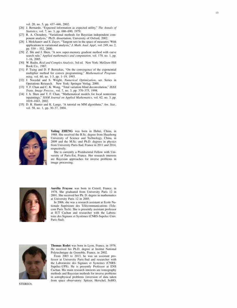
Yuling ZHENG was born in Hubei, China, in1988. She received the B.Sc. degree from HuazhongUniversity of Science and Technology, China, in2009 and the M.Sc. and Ph.D. degrees in physicsfrom University Paris-Sud, France in 2011 and 2014,respectively.

She is currently a Postdoctoral Fellow with Uni-versity of Paris-Est, France. Her research interestsare Bayesian approaches for inverse problems inimage processing.

Aurelia Fraysse was born in Creteil, France, in1978. She graduated from University Paris 12 in2001. She received her Ph. D. degree in mathematicsat University Paris 12 in 2005.

In 2006, she was a research assistant at Ecole Na-tionale Superieure des Telecommunications (Tele-com Paris Tech). She is presently assistant professorat IUT Cachan and researcher with the Labora-toire des Signaux et Systemes (CNRS-Supelec-Univ.Paris-Sud).

Thomas Rodet was born in Lyon, France, in 1976.He received his Ph.D. degree at Institut NationalPolytechnique de Grenoble, France, in 2002.

From 2003 to 2013, he was an assistant pro-fessor at University Paris-Sud and researcher withthe Laboratoire des Signaux et Systemes (CNRS-Supelec-UPS). He is presently Professor at ENSCachan. His main research interests are tomographymethods and Bayesian methods for inverse problemsin astrophysical problems (inversion of data takenfrom space observatory: Spitzer, Herschel, SoHO,

STEREO).