


Languages
Pages
Legal

EEL 6537 – Spectral Estimation
Jian Li
Department of Electrical and Computer Engineering
University of Florida
Gainesville, FL 32611, USA
1

“ Spectral Estimation is · · · an Art ”
Petre Stoica
“ I hear, I forget;
I see, I remember;
I do, I understand.”
A Chinese Philosopher.
2

What is Spectral Estimation?
From a finite record of a stationary data sequence, estimate how
the total power is distributed over frequencies , or more practically,
over narrow spectral bands (frequency bins).
3

Spectral Estimation Methods:
• Classical (Nonparametric) Methods
Ex. Pass the data through a set of band-pass filters and measure
the filter output powers.
• Parametric (Modern) Approaches
Ex. Model the data as a sum of a few damped sinusoids and
estimate their parameters.
Trade-Offs: (Robustness vs. Accuracy)
• Parametric Methods may offer better estimates if data closely
agrees with assumed model.
• Otherwise, Nonparametric Methods may be better.
4

Some Applications of Spectral Estimation
• Speech
- Formant estimation (for speech recognition)
- Speech coding or compression
• Radar and Sonar
- Source localization with sensor arrays
- Synthetic aperture radar imaging and feature extraction
• Electromagnetics
- Resonant frequencies of a cavity
• Communications
- Code-timing estimation in DS-CDMA systems
5
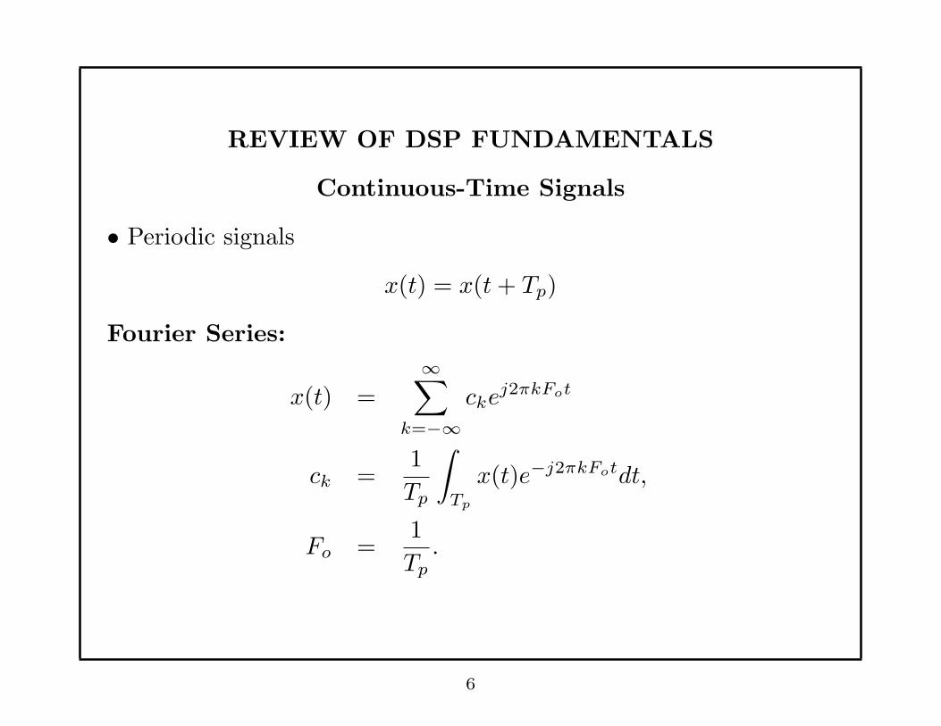
REVIEW OF DSP FUNDAMENTALS
Continuous-Time Signals
• Periodic signals
x(t) = x(t+ Tp)
Fourier Series:
x(t) =
∞∑
k=−∞cke
j2πkFot
ck =1
Tp
∫
Tp
x(t)e−j2πkFotdt,
Fo =1
Tp
.
6
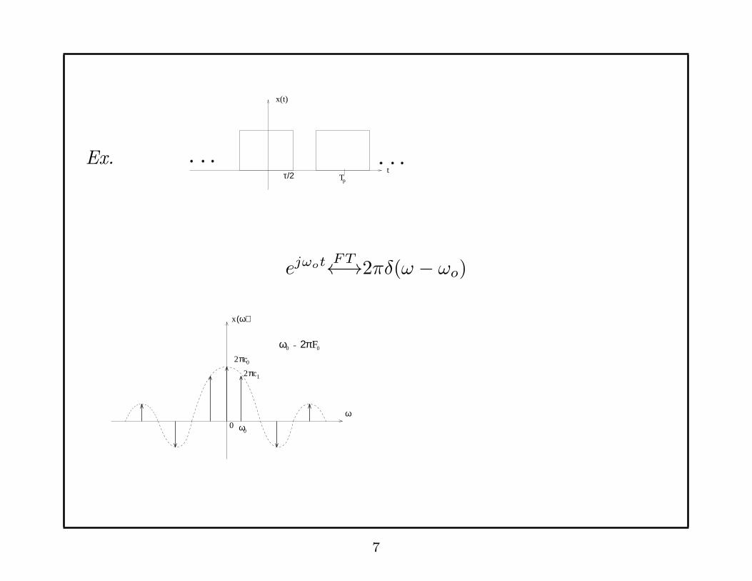
Ex.p
x(t)
τ/2 Tt
ejωot FT←→2πδ(ω − ωo)
π2 c
2πc 1
0
x(ω)
ω
ω
ω = 2πF00
0
0
7
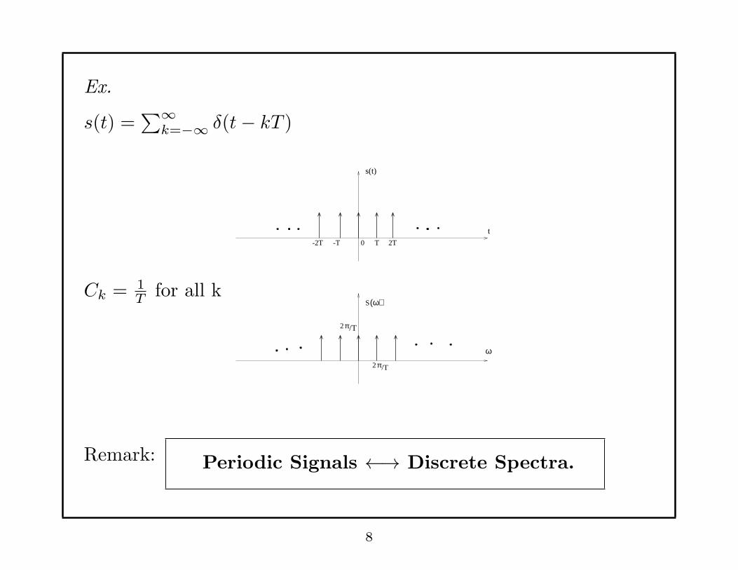
Ex.
s(t) =∑∞
k=−∞ δ(t− kT )
Ck = 1T
for all k
-2T 0-T T 2T
s(t)
t
π/T2
S(ω)
ω
2π/T
Remark: Periodic Signals ←→ Discrete Spectra.
8

• Discrete signals
Ex:
T
x(t)
x(t) s(t)
t
(ω)x
ω
ωt
2π/Τ
Remark: Discrete Signals ←→ Periodic Spectra.
Discrete Periodic Signals ←→ Periodic Discrete Spectra.
9
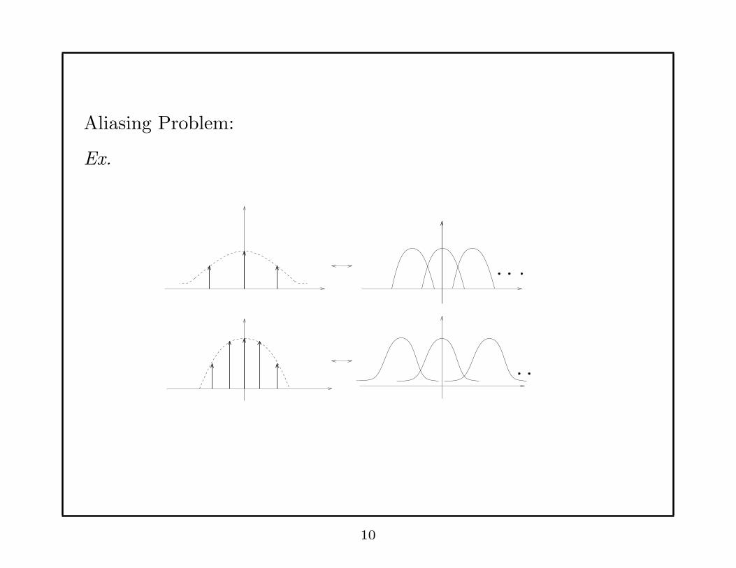
Aliasing Problem:
Ex.
10
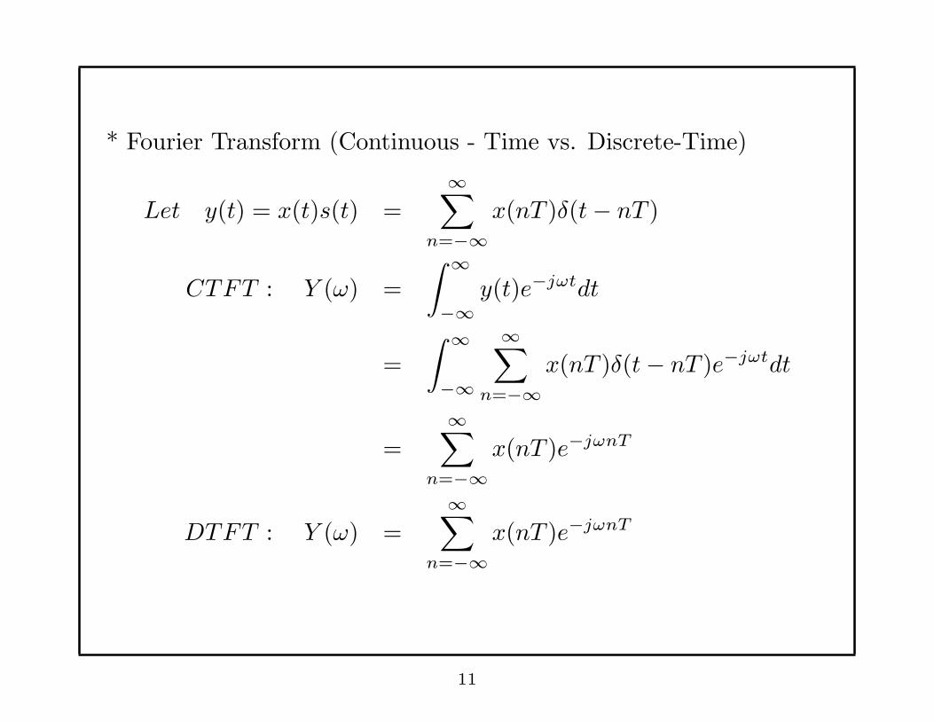
* Fourier Transform (Continuous - Time vs. Discrete-Time)
Let y(t) = x(t)s(t) =
∞∑
n=−∞x(nT )δ(t− nT )
CTFT : Y (ω) =
∫ ∞
−∞y(t)e−jωtdt
=
∫ ∞
−∞
∞∑
n=−∞x(nT )δ(t− nT )e−jωtdt
=
∞∑
n=−∞x(nT )e−jωnT
DTFT : Y (ω) =
∞∑
n=−∞x(nT )e−jωnT
11
SignalDiscrete-Time x(nT)
nT ω
T0
DTFT
y(ω)
2 πT
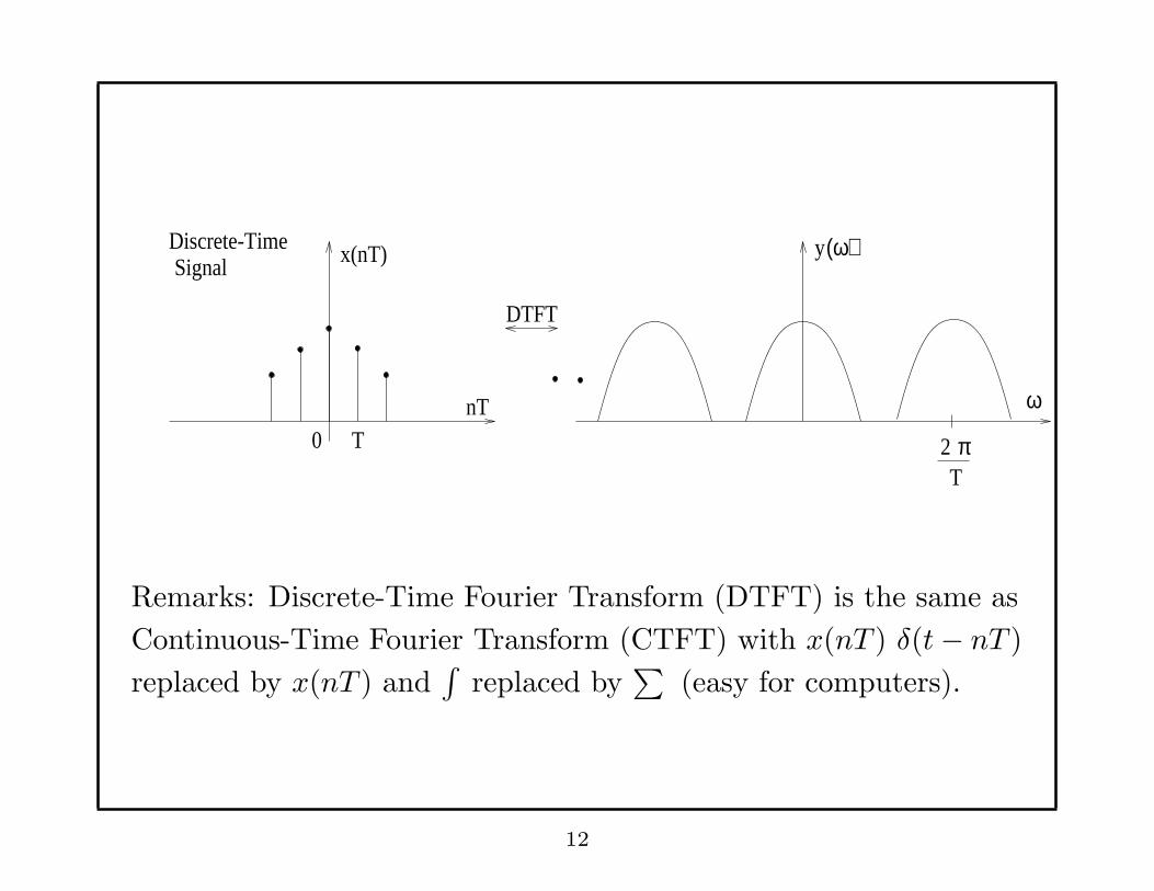
Remarks: Discrete-Time Fourier Transform (DTFT) is the same as
Continuous-Time Fourier Transform (CTFT) with x(nT ) δ(t− nT )
replaced by x(nT ) and∫
replaced by∑
(easy for computers).
12
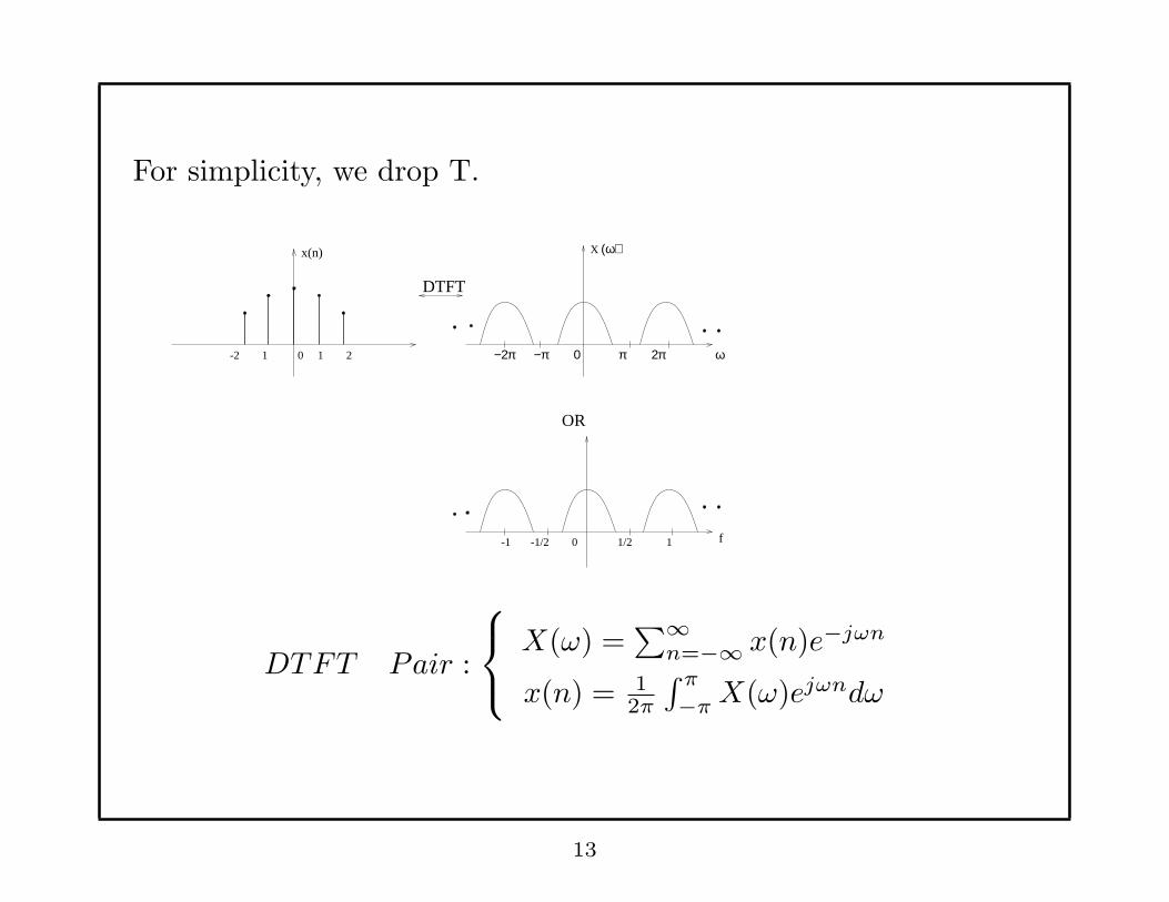
For simplicity, we drop T.
-2 1
-1 -1/2 0 1/2 1
Xx(n)
DTFT
(ω)
ω
OR
f
0 1 2 −2π −π 0 π 2π
DTFT Pair :
X(ω) =∑∞
n=−∞ x(n)e−jωn
x(n) = 12π
∫ π
−πX(ω)ejωndω
13
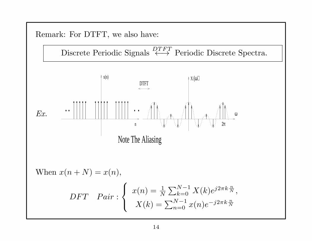
Remark: For DTFT, we also have:
Discrete Periodic SignalsDTFT←→ Periodic Discrete Spectra.
Ex.
x(n)
2πn
DTFTX (ω)
ω
Note The Aliasing
When x(n+N) = x(n),
DFT Pair :
x(n) = 1N
∑N−1k=0 X(k)ej2πk n
N ,
X(k) =∑N−1
n=0 x(n)e−j2πk nN
14
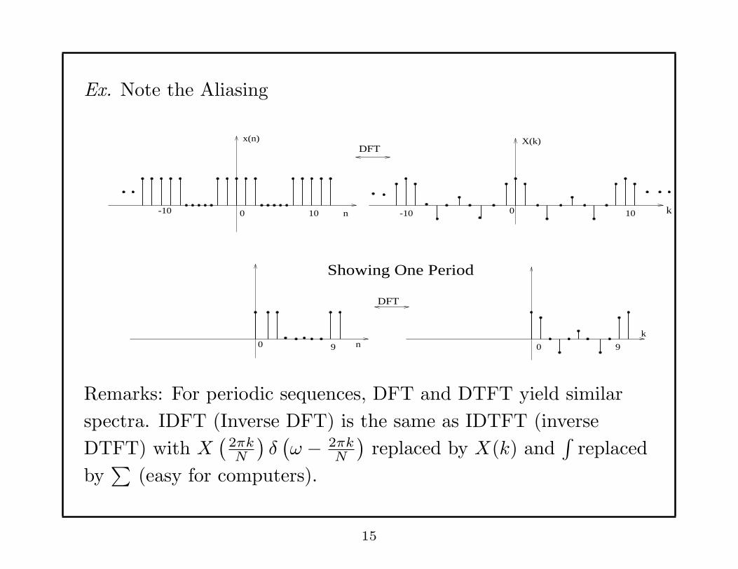
Ex. Note the Aliasing
x(n)
n
0 9 0 9
k
X(k)
-10 0 1010-10 0
n
DFT
DFT
k
Showing One Period
Remarks: For periodic sequences, DFT and DTFT yield similar
spectra. IDFT (Inverse DFT) is the same as IDTFT (inverse
DTFT) with X(
2πkN
)δ(ω − 2πk
N
)replaced by X(k) and
∫replaced
by∑
(easy for computers).
15

Effects of Zero-Padding:
x(n)
n
x(n)
x(n)
n
n
DTFT
10 points
5 points
0
X(k)
0 1 2 3 4 k
0
X(k)
1 2
3 4
5 6
7 89 k
2π ω
X (ω)
DFT
DFT
Remark:• The more zeroes padded, the closer X(k) is to X(ω).
• X(k) is a sampled version of X(ω) for finite duration sequences.
16
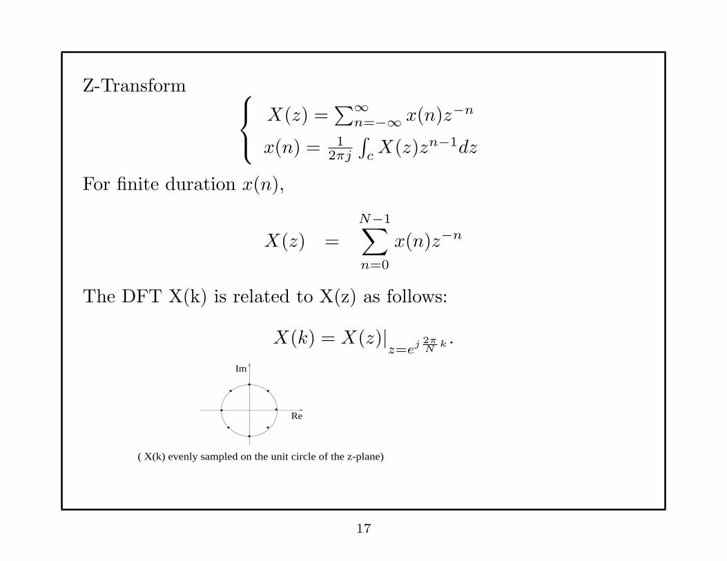
Z-Transform
X(z) =∑∞
n=−∞ x(n)z−n
x(n) = 12πj
∫
cX(z)zn−1dz
For finite duration x(n),
X(z) =
N−1∑
n=0
x(n)z−n
The DFT X(k) is related to X(z) as follows:
X(k) = X(z)|z=e
j 2πN
k .
Im
Re
( X(k) evenly sampled on the unit circle of the z-plane)
17
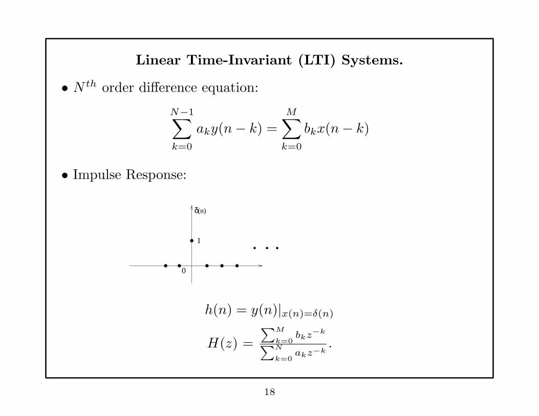
Linear Time-Invariant (LTI) Systems.
• N th order difference equation:
N−1∑
k=0
aky(n− k) =
M∑
k=0
bkx(n− k)
• Impulse Response:
δ
1
0
(n)
h(n) = y(n)|x(n)=δ(n)
H(z) =
∑M
k=0bkz−k
∑N
k=0akz−k
.
18

• Bounded-Input Bounded-Output (BIBO) Stability:
All poles of H(z) are inside the unit circle for a causal system
(where h(n)=0, n< 0).
• FIR Filter: N=0.
• IIR Filter: N>0.
• Minimum Phase: All poles and zeroes of H(z) are inside the unit
circle.
19
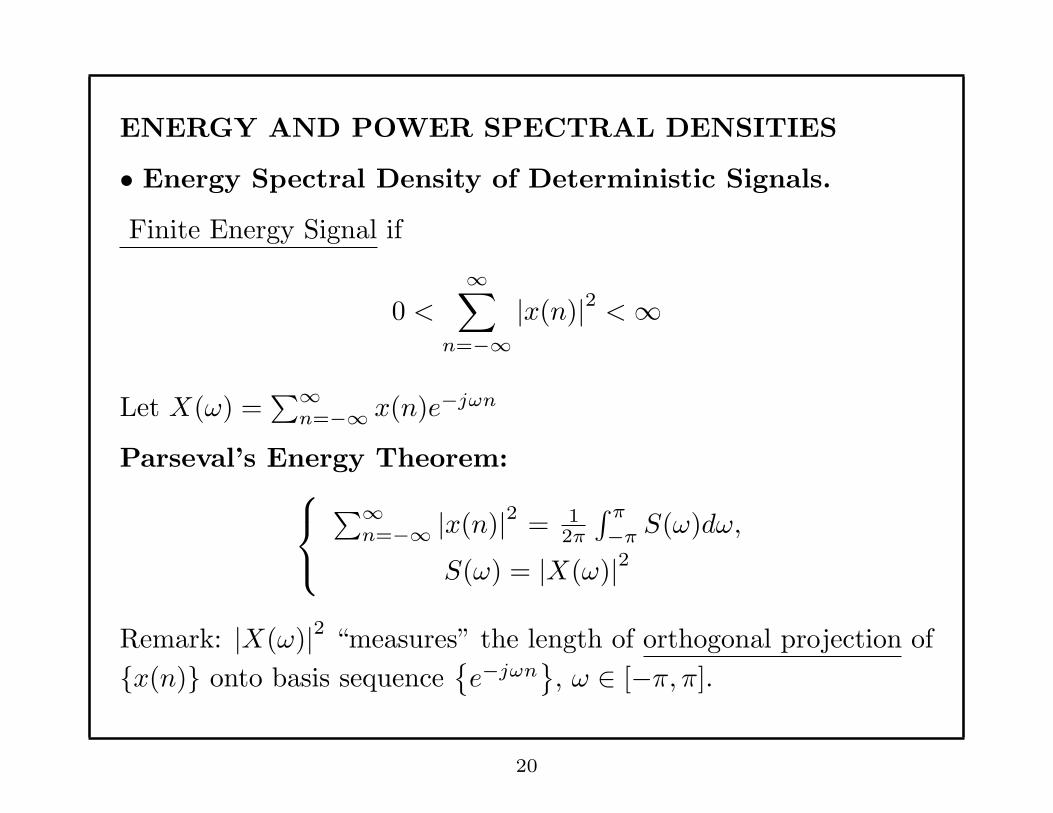
ENERGY AND POWER SPECTRAL DENSITIES
• Energy Spectral Density of Deterministic Signals.
Finite Energy Signal if
0 <∞∑
n=−∞|x(n)|2 <∞
Let X(ω) =∑∞
n=−∞ x(n)e−jωn
Parseval’s Energy Theorem:
∑∞n=−∞ |x(n)|2 = 1
2π
∫ π
−πS(ω)dω,
S(ω) = |X(ω)|2
Remark: |X(ω)|2 “measures” the length of orthogonal projection of
{x(n)} onto basis sequence{e−jωn
}, ω ∈ [−π, π].
20

Let ρ(k) =∑∞
n=−∞ x(n)x∗(n− k).
∞∑
k=−∞ρ(k)e−jωk =
∞∑
k=−∞
∞∑
n=−∞x(n)x∗(n− k)e−jωnejω(n−k)
=
[ ∞∑
n=−∞x(n)e−jωn
][ ∞∑
s=−∞x(s)e−jωs
]∗
= |X(ω)|2 = S(ω).
Remark: S(ω) is the DTFT of the “autocorrelation” of finite
energy sequence {x(n) }.
21
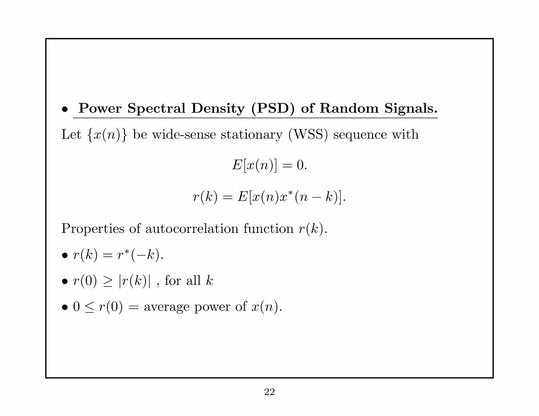
• Power Spectral Density (PSD) of Random Signals.
Let {x(n)} be wide-sense stationary (WSS) sequence with
E[x(n)] = 0.
r(k) = E[x(n)x∗(n− k)].
Properties of autocorrelation function r(k).
• r(k) = r∗(−k).• r(0) ≥ |r(k)| , for all k
• 0 ≤ r(0) = average power of x(n).
22
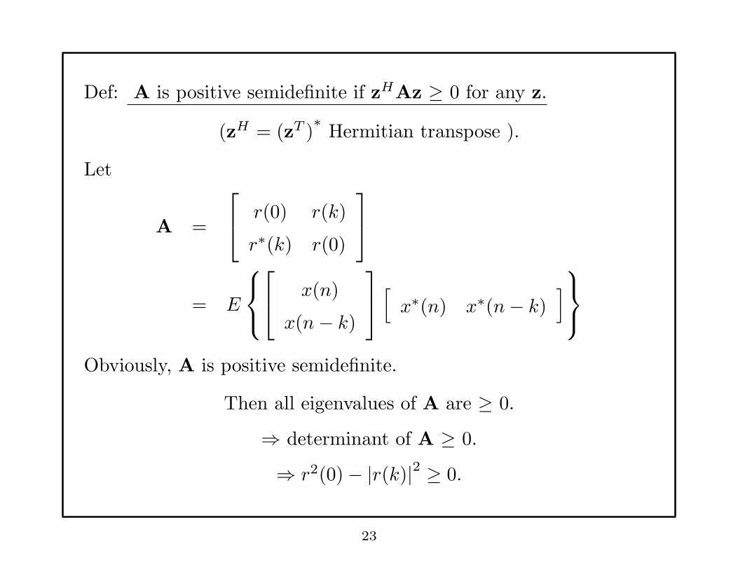
Def: A is positive semidefinite if zHAz ≥ 0 for any z.
(zH = (zT )∗
Hermitian transpose ).
Let
A =
r(0) r(k)
r∗(k) r(0)
= E
x(n)
x(n− k)
[
x∗(n) x∗(n− k)]
Obviously, A is positive semidefinite.
Then all eigenvalues of A are ≥ 0.
⇒ determinant of A ≥ 0.
⇒ r2(0)− |r(k)|2 ≥ 0.
23
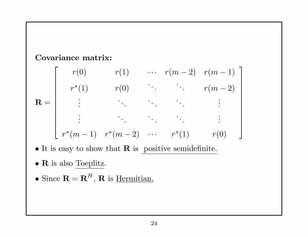
Covariance matrix:
R =
r(0) r(1) · · · r(m− 2) r(m− 1)
r∗(1) r(0). . .
. . . r(m− 2)...
. . .. . .
. . ....
.... . .
. . .. . .
...
r∗(m− 1) r∗(m− 2) · · · r∗(1) r(0)
• It is easy to show that R is positive semidefinite.
• R is also Toeplitz.
• Since R = RH , R is Hermitian.
24
• Eigendecomposition of R
R = UΣUH ,
where UHU = UUH = I
(U is unitary matrix whose columns are eigenvectors of R)
Σ= diag(λ1, ..., λm ),
(λi are the eigenvalues of R, real, and ≥ 0).
25
First Definition of PSD:
P (ω) =∞∑
k=−∞r(k)e−jωk
r(k) =1
2π
∫ π
−π
P (ω)ejωkdω
Or
P (f) =
∞∑
k=−∞r(k)e−j2πfk
r(k) =
∫ 12
− 12
P (f)ej2πfkdf
Remark: • Since r(k) is discrete, P (ω) and P (f) are periodic, with
period 2π (ω) and 1 (f), respectively.
• We usually consider ω ∈ [−π, π] or f ∈ [− 12 ,
12 ].
26
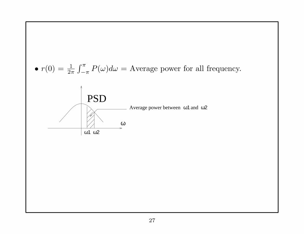
• r(0) = 12π
∫ π
−πP (ω)dω = Average power for all frequency.
PSD
ω1 ω2
ω
Average power between ω1 and ω2
27
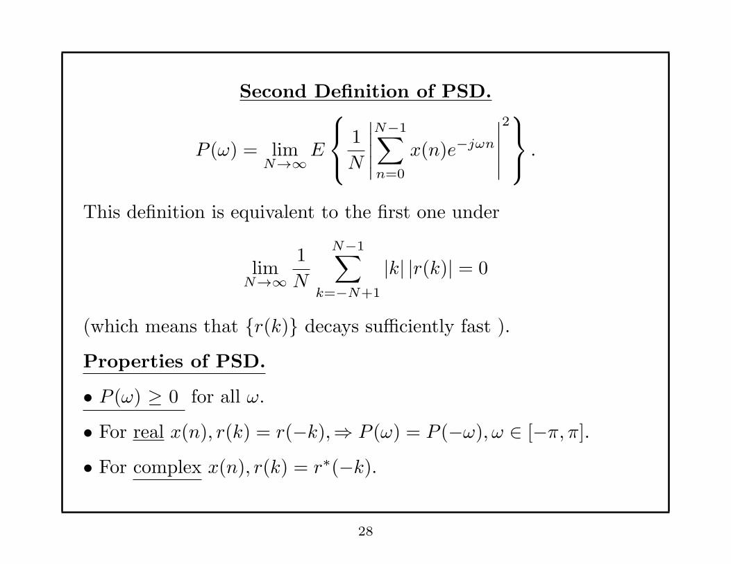
Second Definition of PSD.
P (ω) = limN→∞
E
1
N
∣∣∣∣∣
N−1∑
n=0
x(n)e−jωn
∣∣∣∣∣
2
.
This definition is equivalent to the first one under
limN→∞
1
N
N−1∑
k=−N+1
|k| |r(k)| = 0
(which means that {r(k)} decays sufficiently fast ).
Properties of PSD.
• P (ω) ≥ 0 for all ω.
• For real x(n), r(k) = r(−k),⇒ P (ω) = P (−ω), ω ∈ [−π, π].
• For complex x(n), r(k) = r∗(−k).
28

PSD for LTI Systems.
x(n) y(n) H (ω)
Py(ω) = Px(ω)|H(ω)|2.
Complex (DE) Modulation.
y(n) = x(n)ejω0n.
It is easy to show that
ry(k) = rx(k)ejω0k.
Py(ω) = Px(ω − ω0).
29
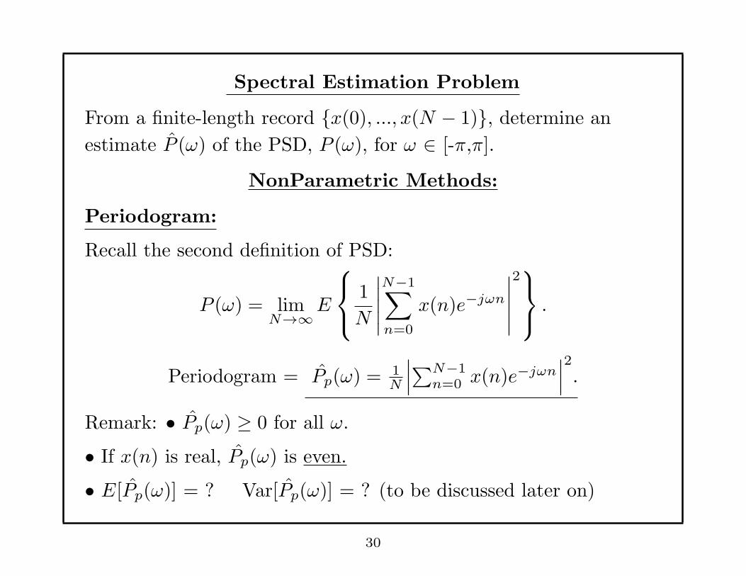
Spectral Estimation Problem
From a finite-length record {x(0), ..., x(N − 1)}, determine an
estimate P (ω) of the PSD, P (ω), for ω ∈ [-π,π].
NonParametric Methods:
Periodogram:
Recall the second definition of PSD:
P (ω) = limN→∞
E
1
N
∣∣∣∣∣
N−1∑
n=0
x(n)e−jωn
∣∣∣∣∣
2
.
Periodogram = Pp(ω) = 1N
∣∣∣∑N−1
n=0 x(n)e−jωn∣∣∣
2
.
Remark: • Pp(ω) ≥ 0 for all ω.
• If x(n) is real, Pp(ω) is even.
• E[Pp(ω)] = ? Var[Pp(ω)] = ? (to be discussed later on)
30
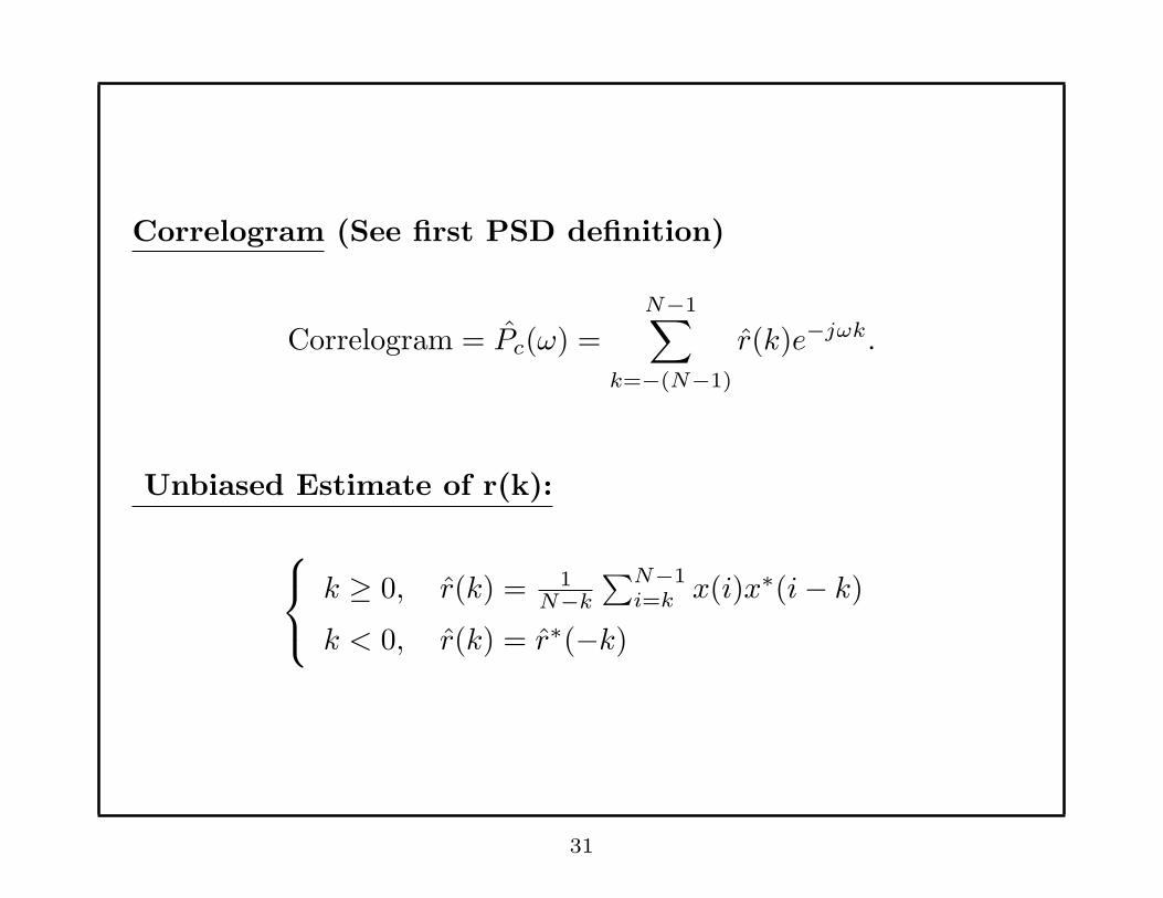
Correlogram (See first PSD definition)
Correlogram = Pc(ω) =
N−1∑
k=−(N−1)
r(k)e−jωk.
Unbiased Estimate of r(k):
k ≥ 0, r(k) = 1N−k
∑N−1i=k x(i)x∗(i− k)
k < 0, r(k) = r∗(−k)
31
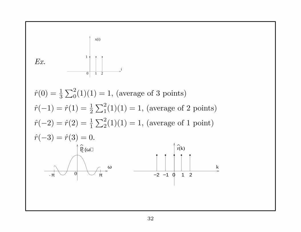
Ex.1
0 1 2i
x(i)
r(0) = 13
∑20(1)(1) = 1, (average of 3 points)
r(−1) = r(1) = 12
∑21(1)(1) = 1, (average of 2 points)
r(−2) = r(2) = 11
∑22(1)(1) = 1, (average of 1 point)
r(−3) = r(3) = 0.
(ω)cp
ω
ππ 0
r(k)
k
- −2 −1 0 1 2
32
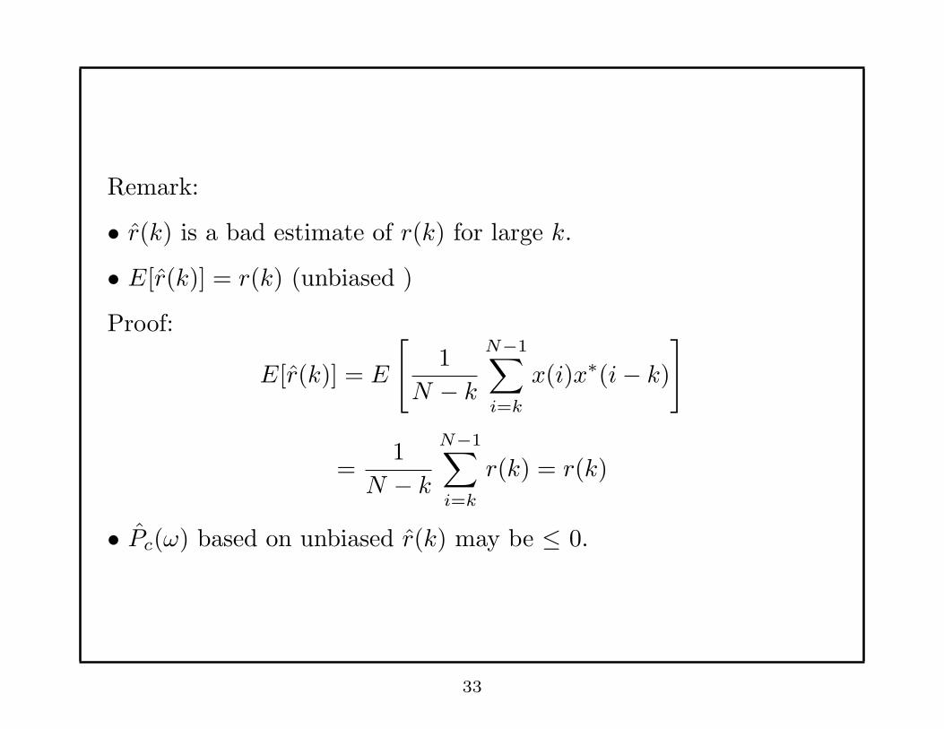
Remark:
• r(k) is a bad estimate of r(k) for large k.
• E[r(k)] = r(k) (unbiased )
Proof:
E[r(k)] = E
[
1
N − k
N−1∑
i=k
x(i)x∗(i− k)]
=1
N − k
N−1∑
i=k
r(k) = r(k)
• Pc(ω) based on unbiased r(k) may be ≤ 0.
33
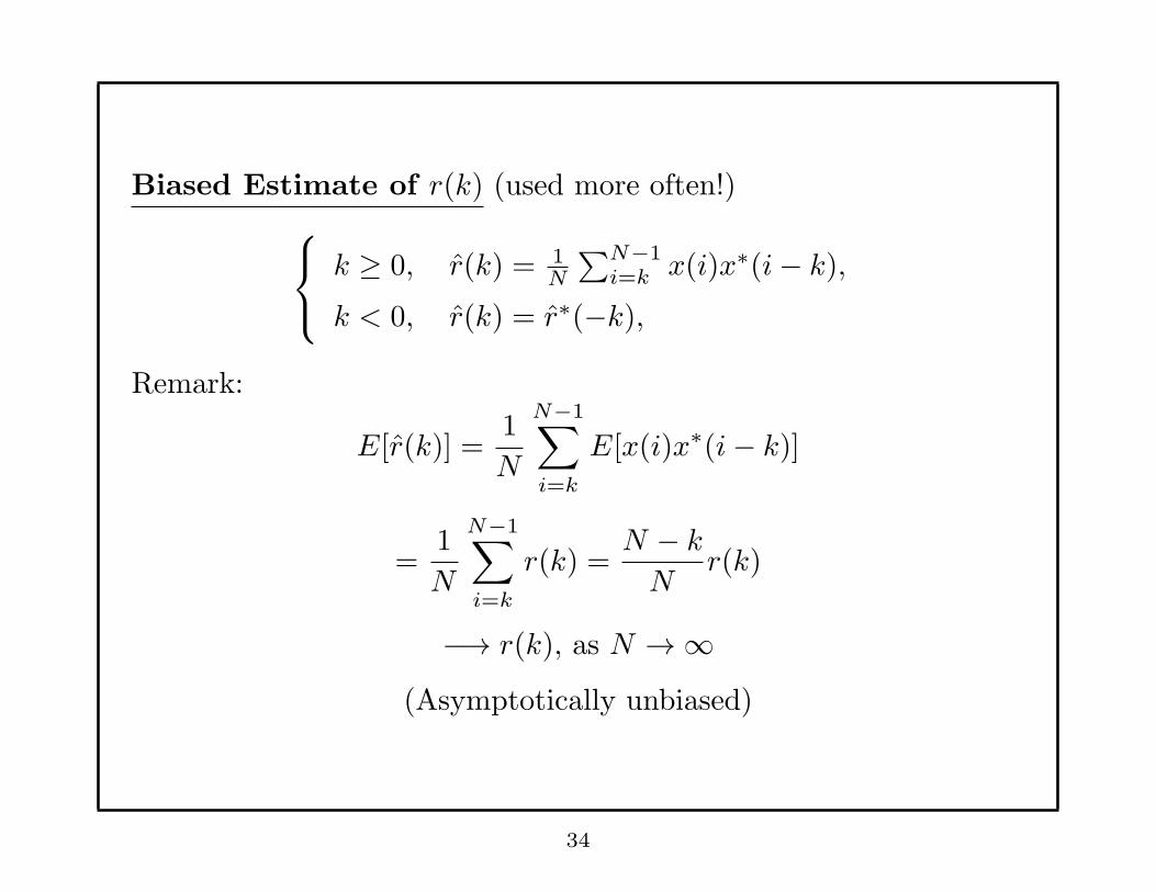
Biased Estimate of r(k) (used more often!)
k ≥ 0, r(k) = 1N
∑N−1i=k x(i)x∗(i− k),
k < 0, r(k) = r∗(−k),
Remark:
E[r(k)] =1
N
N−1∑
i=k
E[x(i)x∗(i− k)]
=1
N
N−1∑
i=k
r(k) =N − kN
r(k)
−→ r(k), as N →∞(Asymptotically unbiased)
34
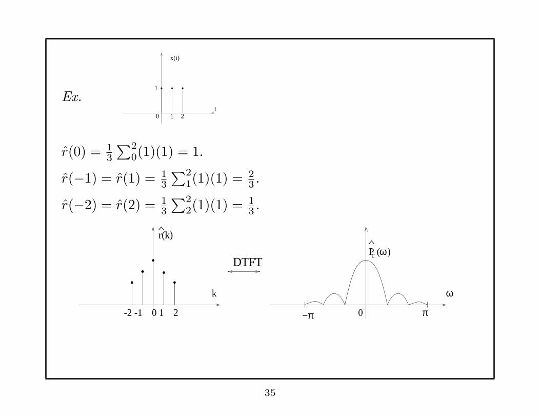
Ex.1
0 1 2i
x(i)
r(0) = 13
∑20(1)(1) = 1.
r(−1) = r(1) = 13
∑21(1)(1) = 2
3 .
r(−2) = r(2) = 13
∑22(1)(1) = 1
3 .
r(k)
-2 -1 0 1 2
k
DTFT
−π π
ω
P (c ω)
0
35
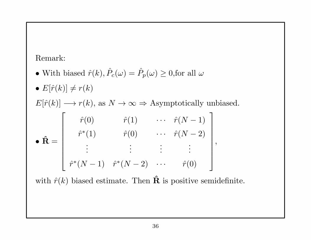
Remark:
• With biased r(k), Pc(ω) = Pp(ω) ≥ 0,for all ω
• E[r(k)] 6= r(k)
E[r(k)] −→ r(k), as N →∞ ⇒ Asymptotically unbiased.
• R =
r(0) r(1) · · · r(N − 1)
r∗(1) r(0) · · · r(N − 2)...
......
...
r∗(N − 1) r∗(N − 2) · · · r(0)
,
with r(k) biased estimate. Then R is positive semidefinite.
36
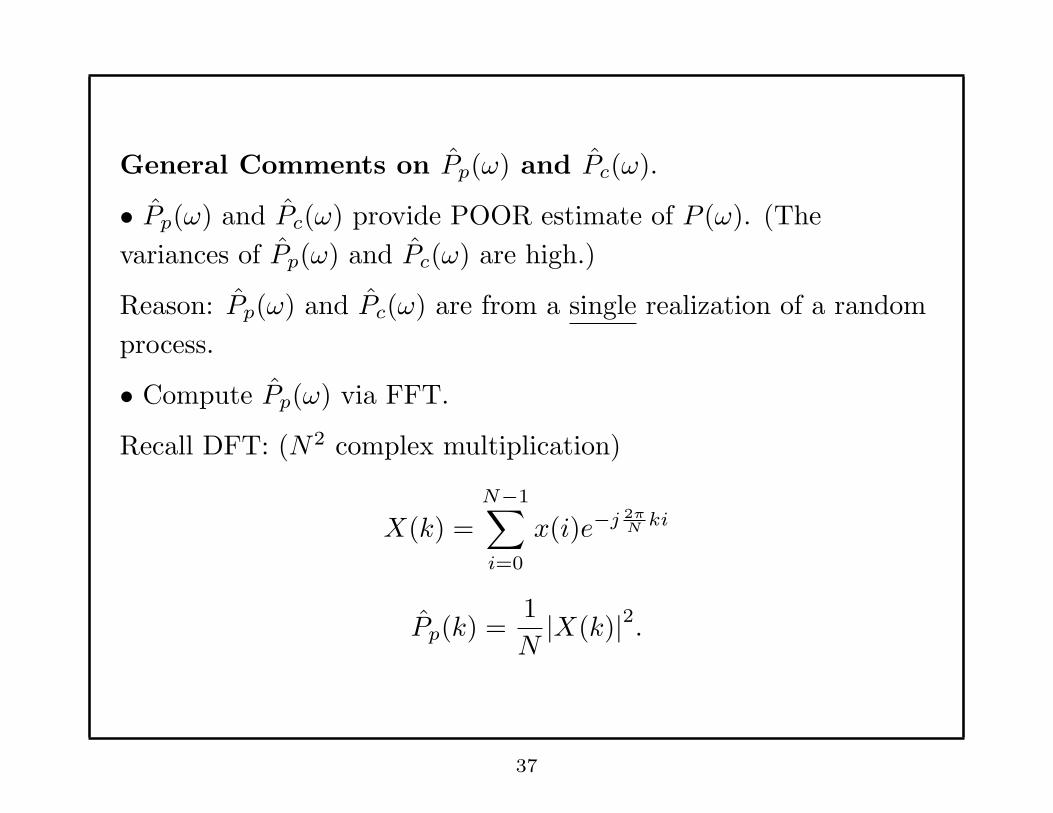
General Comments on Pp(ω) and Pc(ω).
• Pp(ω) and Pc(ω) provide POOR estimate of P (ω). (The
variances of Pp(ω) and Pc(ω) are high.)
Reason: Pp(ω) and Pc(ω) are from a single realization of a random
process.
• Compute Pp(ω) via FFT.
Recall DFT: (N2 complex multiplication)
X(k) =N−1∑
i=0
x(i)e−j 2πN
ki
Pp(k) =1
N|X(k)|2.
37
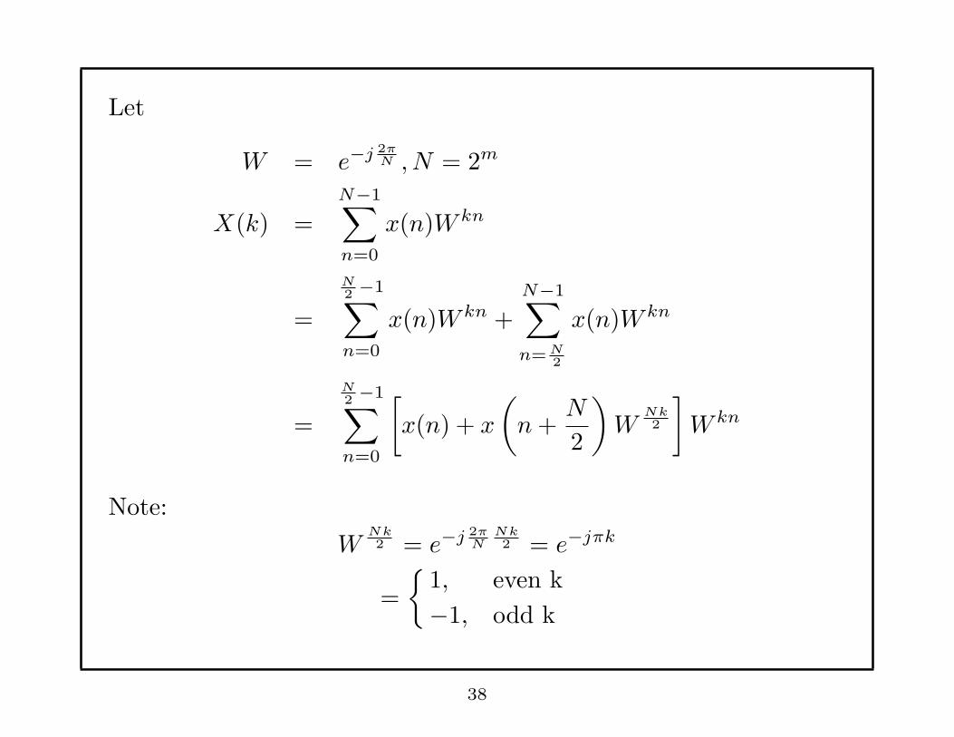
Let
W = e−j 2πN , N = 2m
X(k) =
N−1∑
n=0
x(n)W kn
=
N2 −1∑
n=0
x(n)W kn +N−1∑
n= N2
x(n)W kn
=
N2 −1∑
n=0
[
x(n) + x
(
n+N
2
)
WNk2
]
W kn
Note:
WNk2 = e−j 2π
NNk2 = e−jπk
=
{1, even k
−1, odd k
38

X(2p) =∑N−1
n=0
[x(n) + x(n+ N
2 )]W kn, k = 2p = 0, 2, ...
X(2p+ 1) =∑N
2 −1n=0
[x(n)− x(n+ N
2 )]W kn, k = 2p+ 1,
which requires 2(
N2
)2complex multiplication
This process is continued till 2 points.
• Remark: An N = 2m -pt FFT requires O(N log2N) complex
multiplications.
• Zero padding may be used so that N = 2m.
• Zero padding will not change resolution of Pp(ω).
39

FUNDAMENTALS OF ESTIMATION THEORY
Properties of a Good Estimator for a constant scalar a
• Small Bias:
Bias = E[a]− a
• Small Variance:
Variance = E{
(a− E[a])2}
• Consistent:
a→ a as Number of measurements →∞.
40
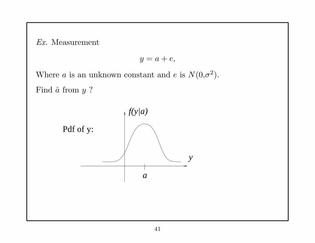
Ex. Measurement
y = a+ e,
Where a is an unknown constant and e is N(0,σ2).
Find a from y ?
Pdf of y:
f(y|a)
y
a
41
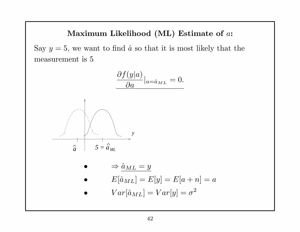
Maximum Likelihood (ML) Estimate of a:
Say y = 5, we want to find a so that it is most likely that the
measurement is 5
∂f(y|a)∂a
|a=aML= 0.
a 5 = a
y
ML
• ⇒ aML = y
• E[aML] = E[y] = E[a+ n] = a
• V ar[aML] = V ar[y] = σ2
42
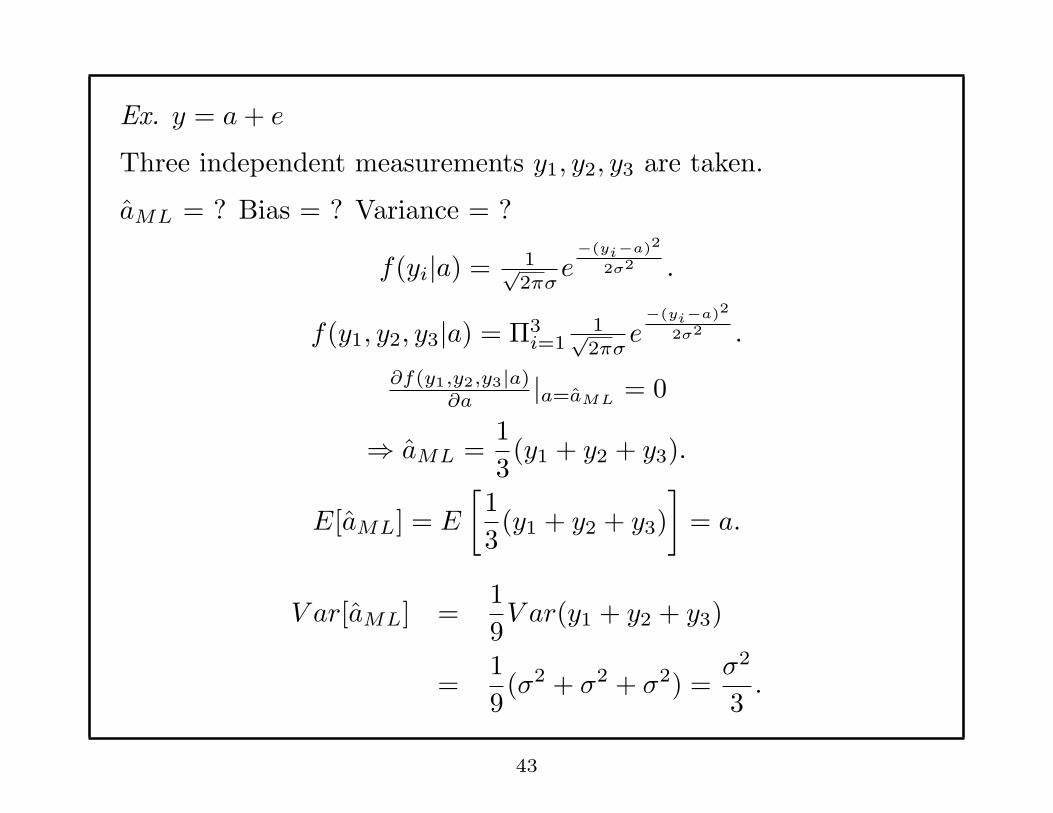
Ex. y = a+ e
Three independent measurements y1, y2, y3 are taken.
aML = ? Bias = ? Variance = ?
f(yi|a) = 1√2πσ
e−(yi−a)2
2σ2 .
f(y1, y2, y3|a) = Π3i=1
1√2πσ
e−(yi−a)2
2σ2 .
∂f(y1,y2,y3|a)∂a
|a=aML= 0
⇒ aML =1
3(y1 + y2 + y3).
E[aML] = E
[1
3(y1 + y2 + y3)
]
= a.
V ar[aML] =1
9V ar(y1 + y2 + y3)
=1
9(σ2 + σ2 + σ2) =
σ2
3.
43

Ex. x is a measurement of an uniformly distributed random
variable on [0, θ ], where θ is an unknown constant. θML = ?
θML = xθ
θθ
= xx
ML
Question: What if two independent measurements x1 and x2 are
taken ?
θML =max (x1, x2 ).x x 1 2
44
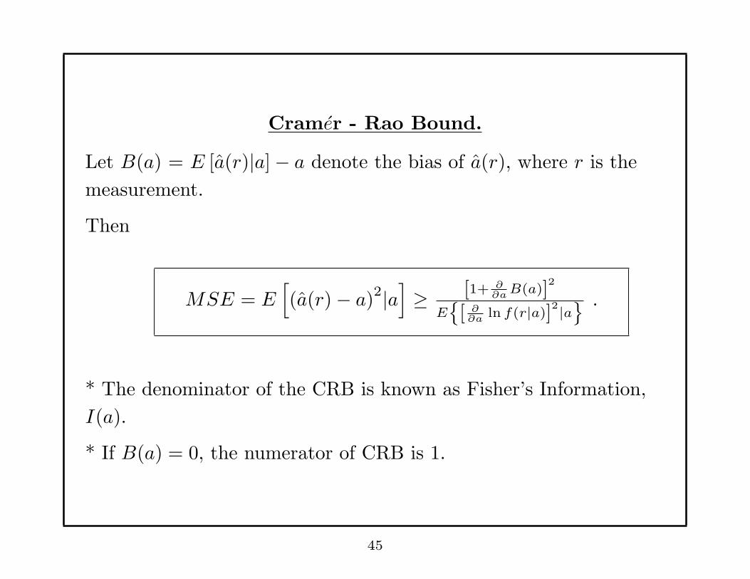
Cramer - Rao Bound.
Let B(a) = E [a(r)|a]− a denote the bias of a(r), where r is the
measurement.
Then
MSE = E[
(a(r)− a)2|a]
≥ [1+ ∂∂a
B(a)]2
E{[ ∂
∂aln f(r|a)]
2|a} .
* The denominator of the CRB is known as Fisher’s Information,
I(a).
* If B(a) = 0, the numerator of CRB is 1.
45
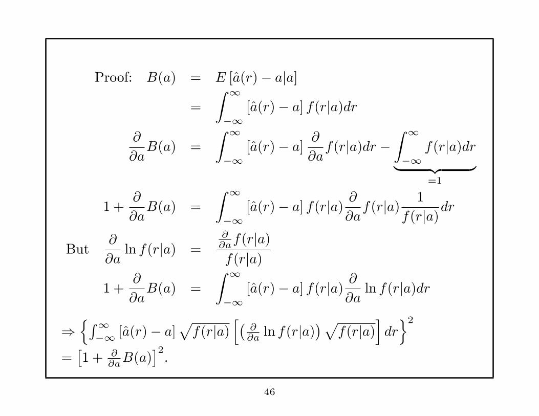
Proof: B(a) = E [a(r)− a|a]
=
∫ ∞
−∞[a(r)− a] f(r|a)dr
∂
∂aB(a) =
∫ ∞
−∞[a(r)− a] ∂
∂af(r|a)dr −
∫ ∞
−∞f(r|a)dr
︸ ︷︷ ︸
=1
1 +∂
∂aB(a) =
∫ ∞
−∞[a(r)− a] f(r|a) ∂
∂af(r|a) 1
f(r|a)dr
But∂
∂aln f(r|a) =
∂∂af(r|a)f(r|a)
1 +∂
∂aB(a) =
∫ ∞
−∞[a(r)− a] f(r|a) ∂
∂aln f(r|a)dr
⇒{∫∞
−∞ [a(r)− a]√
f(r|a)[(
∂∂a
ln f(r|a))√
f(r|a)]
dr}2
=[1 + ∂
∂aB(a)
]2.
46
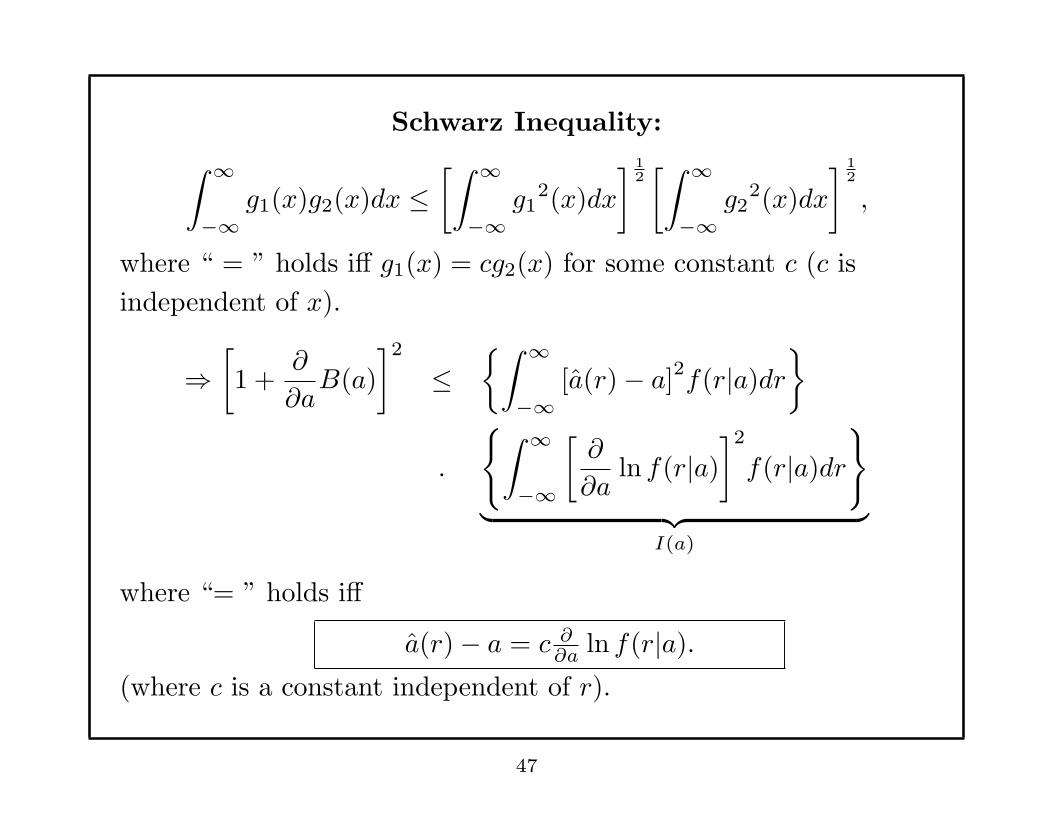
Schwarz Inequality:
∫ ∞
−∞g1(x)g2(x)dx ≤
[∫ ∞
−∞g1
2(x)dx
] 12[∫ ∞
−∞g2
2(x)dx
] 12
,
where “ = ” holds iff g1(x) = cg2(x) for some constant c (c is
independent of x).
⇒[
1 +∂
∂aB(a)
]2
≤{∫ ∞
−∞[a(r)− a]2f(r|a)dr
}
.
{∫ ∞
−∞
[∂
∂aln f(r|a)
]2
f(r|a)dr}
︸ ︷︷ ︸
I(a)
where “= ” holds iff
a(r)− a = c ∂∂a
ln f(r|a).(where c is a constant independent of r).
47
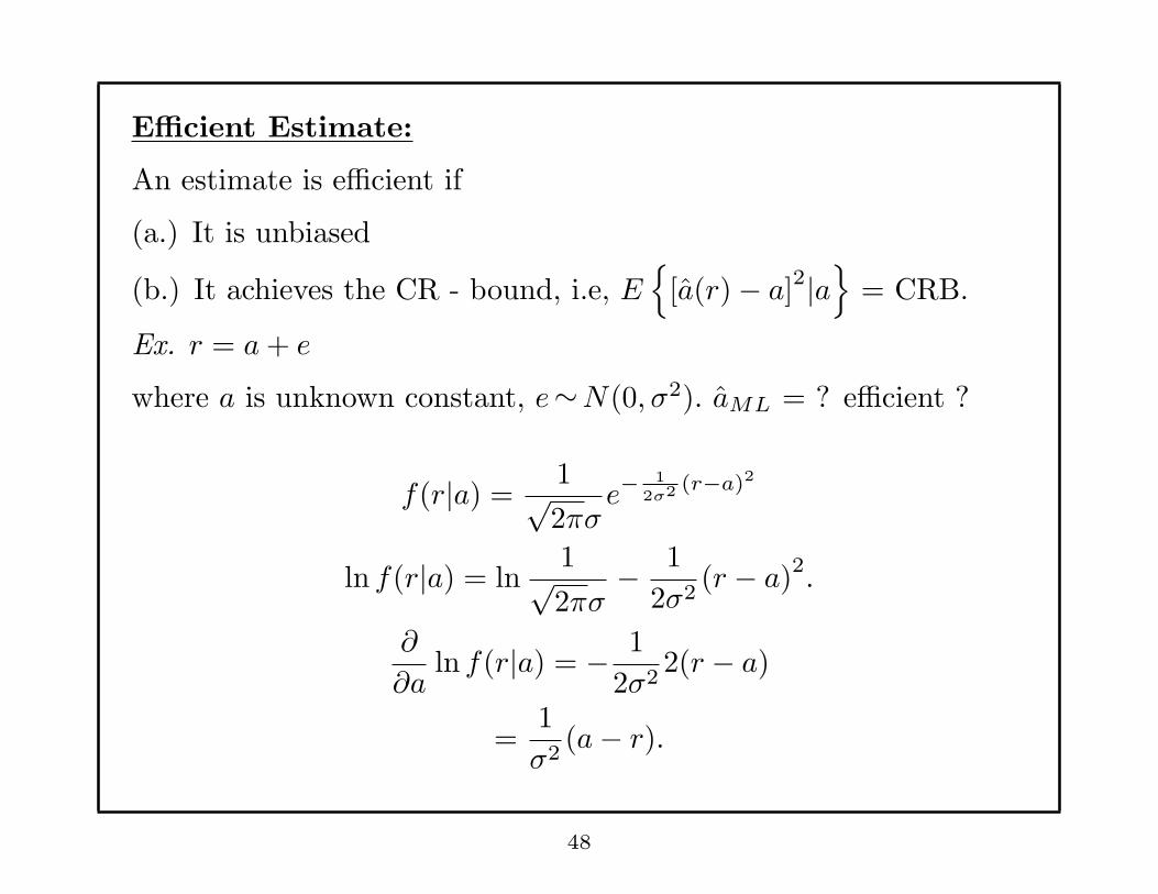
Efficient Estimate:
An estimate is efficient if
(a.) It is unbiased
(b.) It achieves the CR - bound, i.e, E{
[a(r)− a]2|a}
= CRB.
Ex. r = a+ e
where a is unknown constant, e∼N(0, σ2). aML = ? efficient ?
f(r|a) =1√2πσ
e− 12σ2 (r−a)2
ln f(r|a) = ln1√2πσ
− 1
2σ2(r − a)2.
∂
∂aln f(r|a) = − 1
2σ22(r − a)
=1
σ2(a− r).
48

∂
∂aln f(r|a)
∣∣∣∣a=aML
= 0 ⇒ aML = r
∂
∂aln f(r|a) =
1
σ2(a− aML)
⇒ −σ2 ∂
∂aln f(r|a) = aML − a
⇒ aML efficient
E[
(aML − a)2∣∣∣ a]
= CRB
E [aML] = E [r] = a, unbiased
Remark: • MSE = V ar[aML] = V ar[r] = σ2.
•I(a) = E
{[∂
∂aln f(r|a)
]2∣∣∣∣∣a
}
= E
{[1
σ2(a− r)
]2}
=1
σ4σ2 =
1
σ2
⇒ CRB =1
I(a)= σ2 = V ar[aML].
49

Remarks:
(1) If a(r) is unbiased, V ar[a(r) ] ≥ CRB.
(2) If an efficient estimate a(r) exists, i.e,
∂
∂aln f(r|a) = c[a(r)− a]. (c is independent of r.)
then
0 =∂
∂aln f(r|a)|a=aML(r) results in aML(r) = a(r).
⇒ If an efficient estimate exists, it is aML.
(3) If an efficient estimate does not exist, how good aML(r) is
depends on each specific problem.
No estimator can achieve the CR-bound. Bounds (for example,
Bhattacharya, Barankin) larger than the CR-bound may be found.
50
Independent measurements r1, ..., rN available, where ri may or
may not be Gaussian.
Assume
aML =1
N
N∑
i=1
ri.
Law of large numbers: aML −→N→∞
a
Central Limit Theorem:
aML has Gaussian distribution as N →∞.
51

Asymptotic Properties of aML(r1, ..., rN )
(a) aML(r1, ..., rN ) −→N→∞
a (aML is a consistent estimate.)
(b) aML is asymptotically efficient.
(c) aML is aymptotically Gaussian.
Ex. r = g−1(a) + e, e∼N(0, σ2). aML =? efficient ?
Let b = g−1(a). Then a = g(b)
∂
∂aln f(r|a) =
1
σ2
(r − g−1(a)
) dg−1(a)
da|a=aML
= 0
aML = g(r) = g(bML).
Invariance property of ML estimator
• If a = g(b) then aML = g(bML).
• aML may not be efficient. aML is not efficient if g(·) is a
nonlinear function.
52
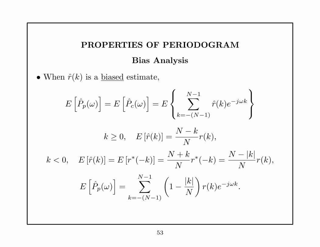
PROPERTIES OF PERIODOGRAM
Bias Analysis
• When r(k) is a biased estimate,
E[
Pp(ω)]
= E[
Pc(ω)]
= E
N−1∑
k=−(N−1)
r(k)e−jωk
k ≥ 0, E [r(k)] =N − kN
r(k),
k < 0, E [r(k)] = E [r∗(−k)] =N + k
Nr∗(−k) =
N − |k|N
r(k),
E[
Pp(ω)]
=
N−1∑
k=−(N−1)
(
1− |k|N
)
r(k)e−jωk.
53
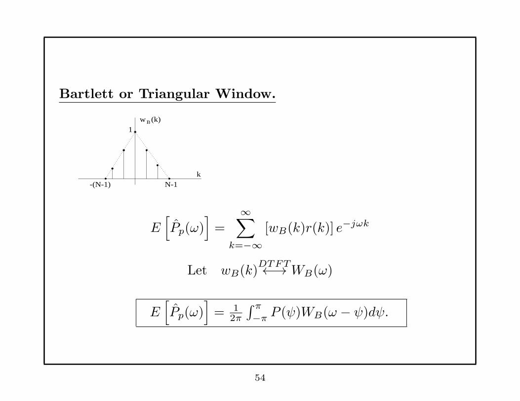
Bartlett or Triangular Window.
N-1k
-(N-1)
1B (k)w
E[
Pp(ω)]
=∞∑
k=−∞[wB(k)r(k)] e−jωk
Let wB(k)DTFT←→ WB(ω)
E[
Pp(ω)]
= 12π
∫ π
−πP (ψ)WB(ω − ψ)dψ.
54

• When r(k) is unbiased estimate,
E[
Pp(ω)]
= 12π
∫ π
−πP (ψ)WR(ω − ψ)dψ .
wR(k)DTFT←→ WR(ω)
N-1
k
-(N-1) 0
(k)R
1
B,R
)ωP( W (ω)
E [ P(ω)]
w
55
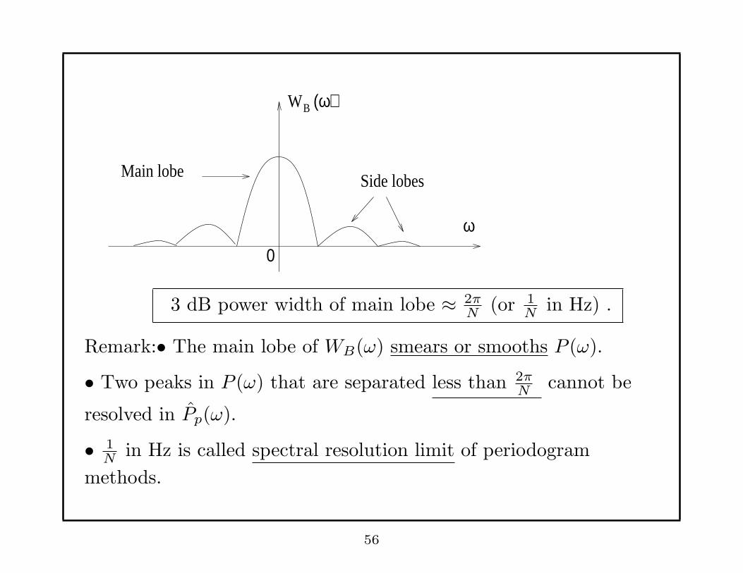
ω
(ω)W B
0
Main lobe Side lobes
3 dB power width of main lobe ≈ 2πN
(or 1N
in Hz) .
Remark:• The main lobe of WB(ω) smears or smooths P (ω).
• Two peaks in P (ω) that are separated less than 2πN
cannot be
resolved in Pp(ω).
• 1N
in Hz is called spectral resolution limit of periodogram
methods.
56
Remark:
• The side lobes of WB(ω) transfer power from high power
frequency bins to low power frequency bins —– leakage.
• Smearing and leakage cause more problems to peaky P (ω) than
to flat P (ω).
If P (ω) = σ2, for all ω, E[Pp(ω)] = P (ω).
• Bias of Pp(ω) decreases as N → ∞. (asymptotically unbiased.)
57
Variance Analysis
We shall consider the case x(n) is zero-mean circularly symmetric
complex Gaussian white noise.
⊙
E[x(n)x∗(k)] = σ2δ(n− k).E[x(n)x(k)] = 0 for all n, k.
⊙is equivalent to:
E [ Re(x(n))Re(x(k))] = σ2
2 δ(n− k).E [Im(x(n))Im(x(k))] = σ2
2 δ(n− k).E [Re(x(n))Im(x(k))] = 0.
Remark: The real and imaginary parts of x(n) are N(0, σ2
2 ) and
independent of each other.
58
Remark: If x(n) is zero-mean complex Gaussian white noise, Pp(ω)
is an unbiased estimate.
• r(k) = σ2δ(k).
E[
Pp(ω)]
=
N−1∑
k=−(N−1)
(
1− |k|N
)
r(k)e−jωk = σ2
• Pp(ω) =
∞∑
k=−∞r(k)e−jωk = σ2
= E[
Pp(ω)]
.
59

For Gaussian complex white noise,
E [x(k)x∗(l)x(m)x∗(n)] = σ4 [δ(k − l)δ(m− n) + δ(k − n)δ(l −m)] .
E[
Pp(ω1)Pp(ω2)]
=1
N2
N−1∑
k=0
N−1∑
l=0
N−1∑
m=0
N−1∑
n=0
E [x(k)x∗(l)x(m)x∗(n)]
e−jω1(k−l)e−jω2(m−n)
= σ4 +σ4
N2
N−1∑
k=0
N−1∑
l=0
e−j(ω1−ω2)(k−l)
= σ4 +σ4
N2
∣∣∣∣∣
N−1∑
k=0
ej(ω1−ω2)k
∣∣∣∣∣
2
= σ4 +σ4
N2
{
sin[(ω1 − ω2)N2 ]
sin (ω1−ω2)2
}2
60
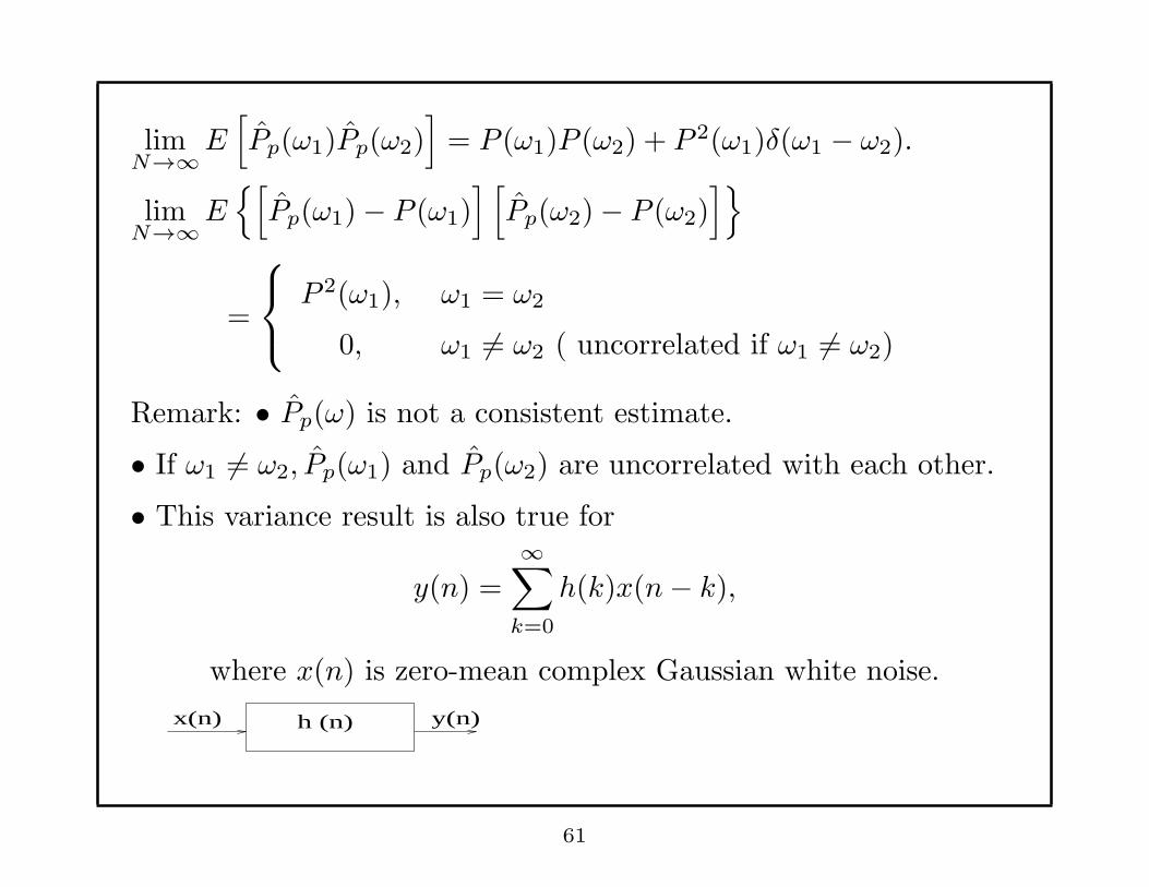
limN→∞
E[
Pp(ω1)Pp(ω2)]
= P (ω1)P (ω2) + P 2(ω1)δ(ω1 − ω2).
limN→∞
E{[
Pp(ω1)− P (ω1)] [
Pp(ω2)− P (ω2)]}
=
P 2(ω1), ω1 = ω2
0, ω1 6= ω2 ( uncorrelated if ω1 6= ω2)
Remark: • Pp(ω) is not a consistent estimate.
• If ω1 6= ω2, Pp(ω1) and Pp(ω2) are uncorrelated with each other.
• This variance result is also true for
y(n) =
∞∑
k=0
h(k)x(n− k),
where x(n) is zero-mean complex Gaussian white noise.
x(n) y(n) h (n)
61
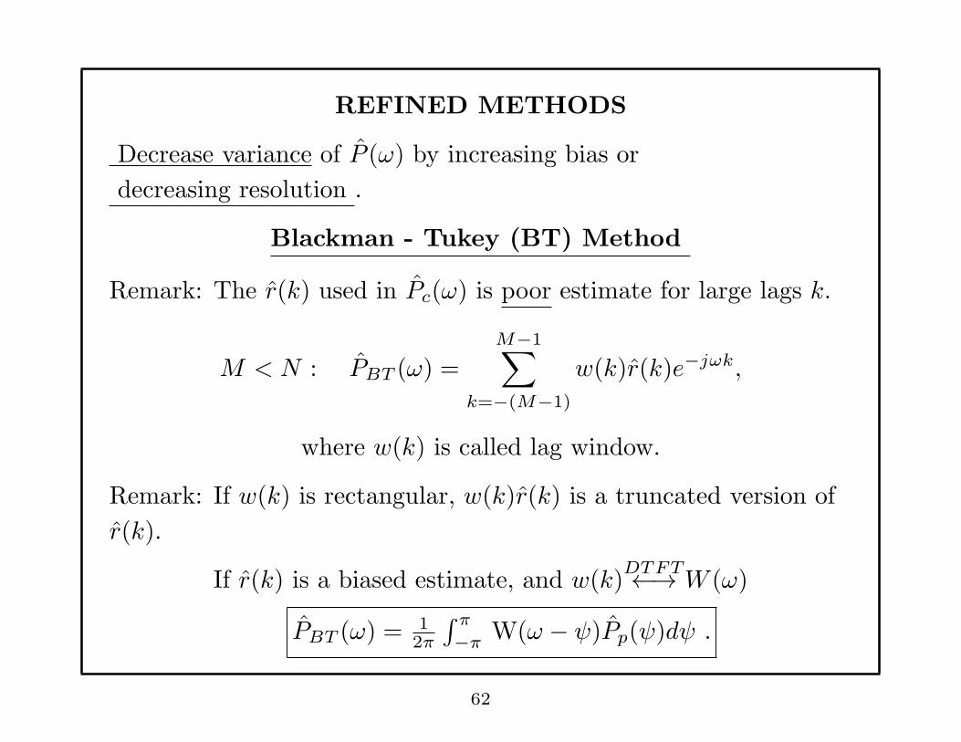
REFINED METHODS
Decrease variance of P (ω) by increasing bias or
decreasing resolution .
Blackman - Tukey (BT) Method
Remark: The r(k) used in Pc(ω) is poor estimate for large lags k.
M < N : PBT (ω) =
M−1∑
k=−(M−1)
w(k)r(k)e−jωk,
where w(k) is called lag window.
Remark: If w(k) is rectangular, w(k)r(k) is a truncated version of
r(k).
If r(k) is a biased estimate, and w(k)DTFT←→ W (ω)
PBT (ω) = 12π
∫ π
−πW(ω − ψ)Pp(ψ)dψ .
62

Remark: • BT spectral estimator is “locally” weighted average of
periodogram Pp(ω).
• The smaller the M , the poorer the resolution of PBT (ω) but the
lower the variance.
• Resolution of PBT (ω) ∝ 1M
.
• Variance of PBT (ω) ∝ MN
M fixed−→N→∞
0 .
• For fixed M , PBT (ω) is asymptotically biased but variance −→ 0.
Question: When is PBT (ω) ≥ 0 ∀ ω?
63

Theorem: Let Y (ω)DTFT←→ y(n), −(N − 1) ≤ n ≤ N − 1
Then Y (ω) ≥ 0 ∀ ω iff
y(0) y(1) · · · y(N − 1) 0 · · ·y(−1) y(0) · · · y(N − 2) y(N − 1) · · ·
.... . .
y[−(N − 1)] · · · y(0) y(1) · · ·
0. . .
. . .. . .
. . .
...
is positive semidefinite.
In other words, Y (ω) ≥ 0 ∀ ω iff
· · · , 0, · · · , 0, y[−(N − 1)], · · · , y(0), y(1), · · · , y(N − 1), 0, · · · is a
positive semidefinite sequence.
64
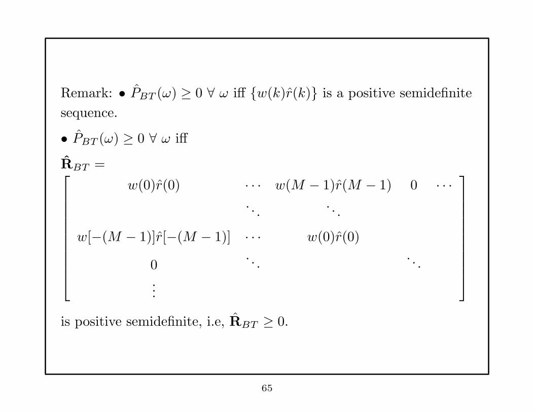
Remark: • PBT (ω) ≥ 0 ∀ ω iff {w(k)r(k)} is a positive semidefinite
sequence.
• PBT (ω) ≥ 0 ∀ ω iff
RBT =
w(0)r(0) · · · w(M − 1)r(M − 1) 0 · · ·. . .
. . .
w[−(M − 1)]r[−(M − 1)] · · · w(0)r(0)
0. . .
. . .
...
is positive semidefinite, i.e, RBT ≥ 0.
65
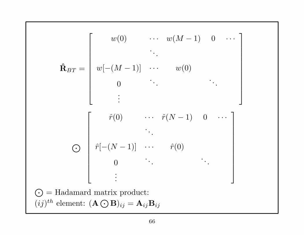
RBT =
w(0) · · · w(M − 1) 0 · · ·. . .
w[−(M − 1)] · · · w(0)
0. . .
. . .
...
⊙
r(0) · · · r(N − 1) 0 · · ·. . .
r[−(N − 1)] · · · r(0)
0. . .
. . .
...
⊙= Hadamard matrix product:
(ij)th element: (A⊙
B)ij = AijBij
66

Theorem:
If A ≥ 0 (positive semidefinite) B ≥ 0 then A⊙
B ≥ 0.
Remark: If r(k) is a biased estimate, Pp(ω) ≥ 0 ∀ ω. Then if W(ω)
≥ 0 ∀ ω, we have PBT (ω) ≥ 0 ∀ ω.
Remark: Nonnegative definite (positive semidefinite) window
sequences: Bartlett, Parzen.
67
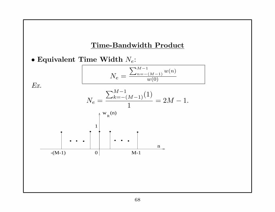
Time-Bandwidth Product
• Equivalent Time Width Ne:
Ne =
∑M−1
n=−(M−1)w(n)
w(0)
Ex.
Ne =
∑M−1k=−(M−1)(1)
1= 2M − 1.
0
1
(n)
n-(M-1) M-1
wR
68
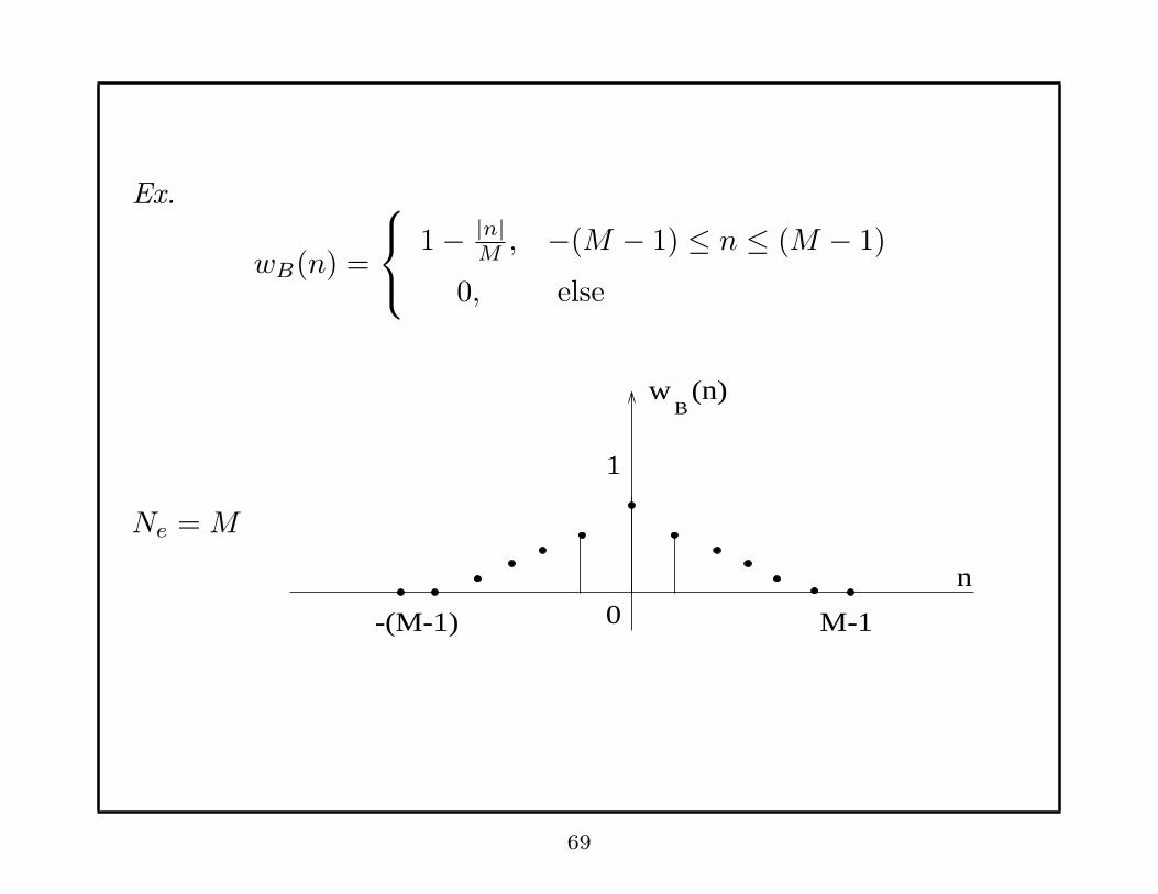
Ex.
wB(n) =
1− |n|M, −(M − 1) ≤ n ≤ (M − 1)
0, else
Ne = M
-(M-1) 0
1
(n)
M-1
n
Bw
69
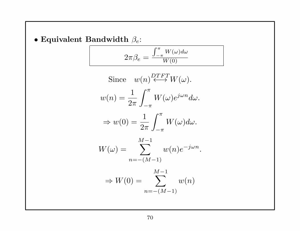
• Equivalent Bandwidth βe:
2πβe =
∫π
−πW (ω)dω
W (0)
Since w(n)DTFT←→ W (ω).
w(n) =1
2π
∫ π
−π
W (ω)ejωndω.
⇒ w(0) =1
2π
∫ π
−π
W (ω)dω.
W (ω) =M−1∑
n=−(M−1)
w(n)e−jωn.
⇒W (0) =
M−1∑
n=−(M−1)
w(n)
70
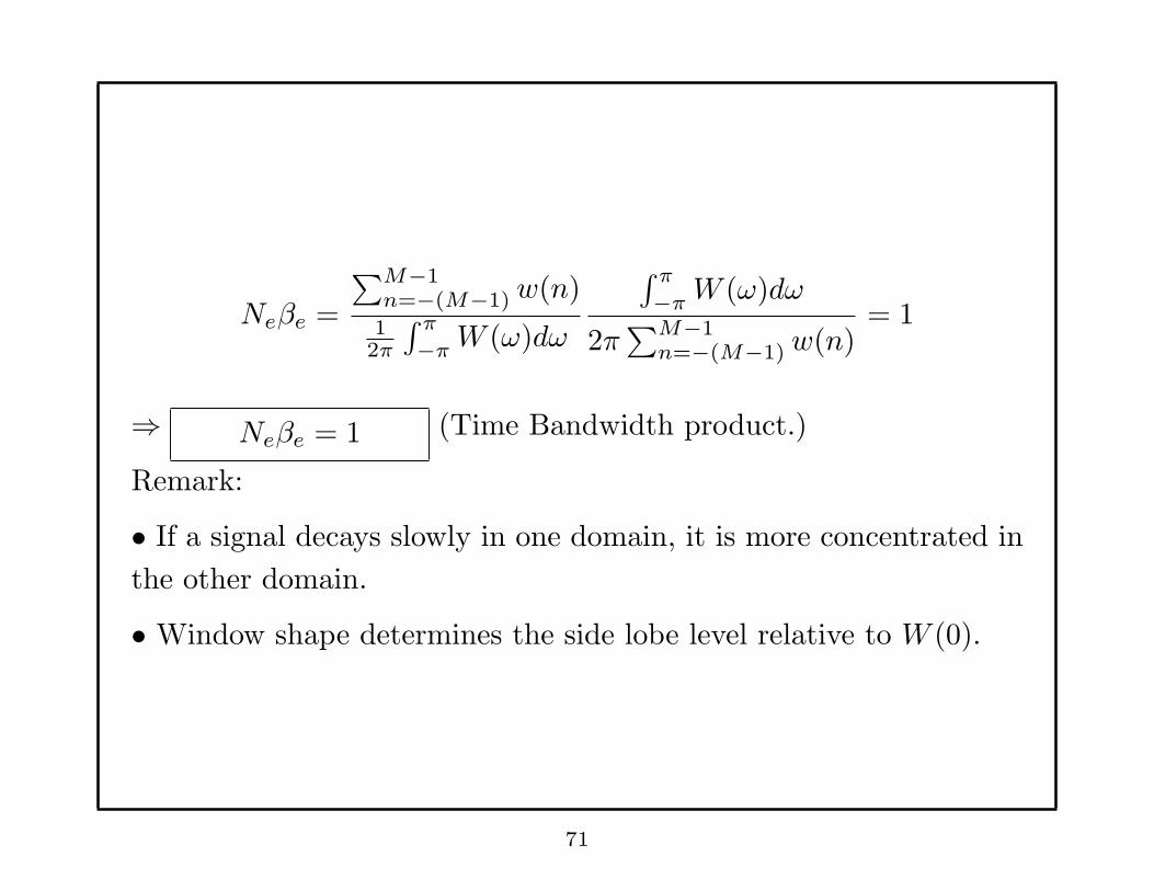
Neβe =
∑M−1n=−(M−1) w(n)
12π
∫ π
−πW (ω)dω
∫ π
−πW (ω)dω
2π∑M−1
n=−(M−1) w(n)= 1
⇒ Neβe = 1 (Time Bandwidth product.)
Remark:
• If a signal decays slowly in one domain, it is more concentrated in
the other domain.
• Window shape determines the side lobe level relative to W (0).
71
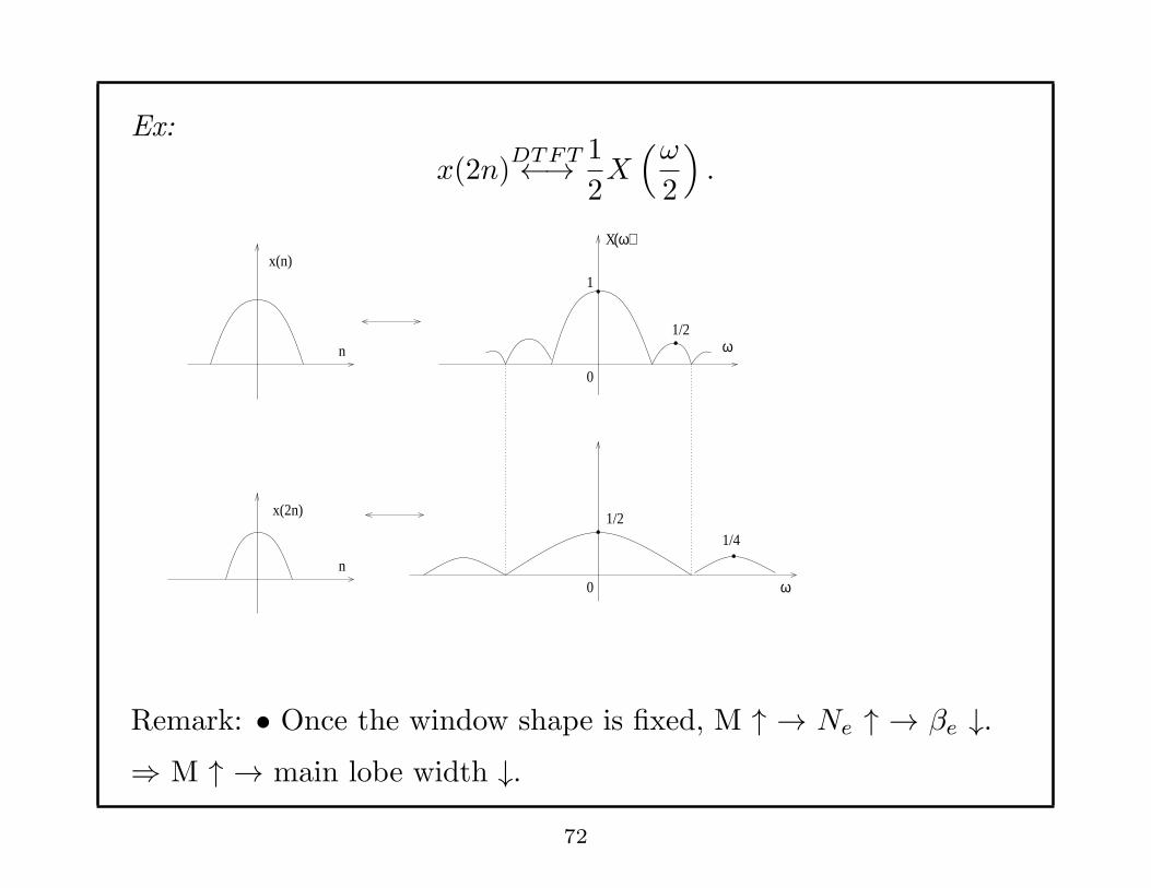
Ex:
x(2n)DTFT←→ 1
2X(ω
2
)
.
x(n)
x(2n)
n
1
0
X(ω)
1/2ω
1/2
0n
ω
1/4
Remark: • Once the window shape is fixed, M ↑ → Ne ↑ → βe ↓.⇒ M ↑ → main lobe width ↓.
72

Window design for PBT (ω)
Let βm = 3dB main lobe width.
Resolution of PBT (ω) ∼ βm Variance of PBT (ω) ∼ 1βm.
• Choice of βm is based on the trade-off between resolution
and variance, and N
• Choice of window shape is based on leakage, and N .
• Practical rule of thumb:
1. M ≤ N10 .
2. Window shape based on trade-off between smearing and leakage.
3. Window shape for PBT (ω) ≥ 0, ∀ωRemark: • Other methods for Non-parametric Spectral
Estimation include: Bartlett, Welch, Daniell Methods.
• All try to reduce variance at the expense of poorer resolution.
73
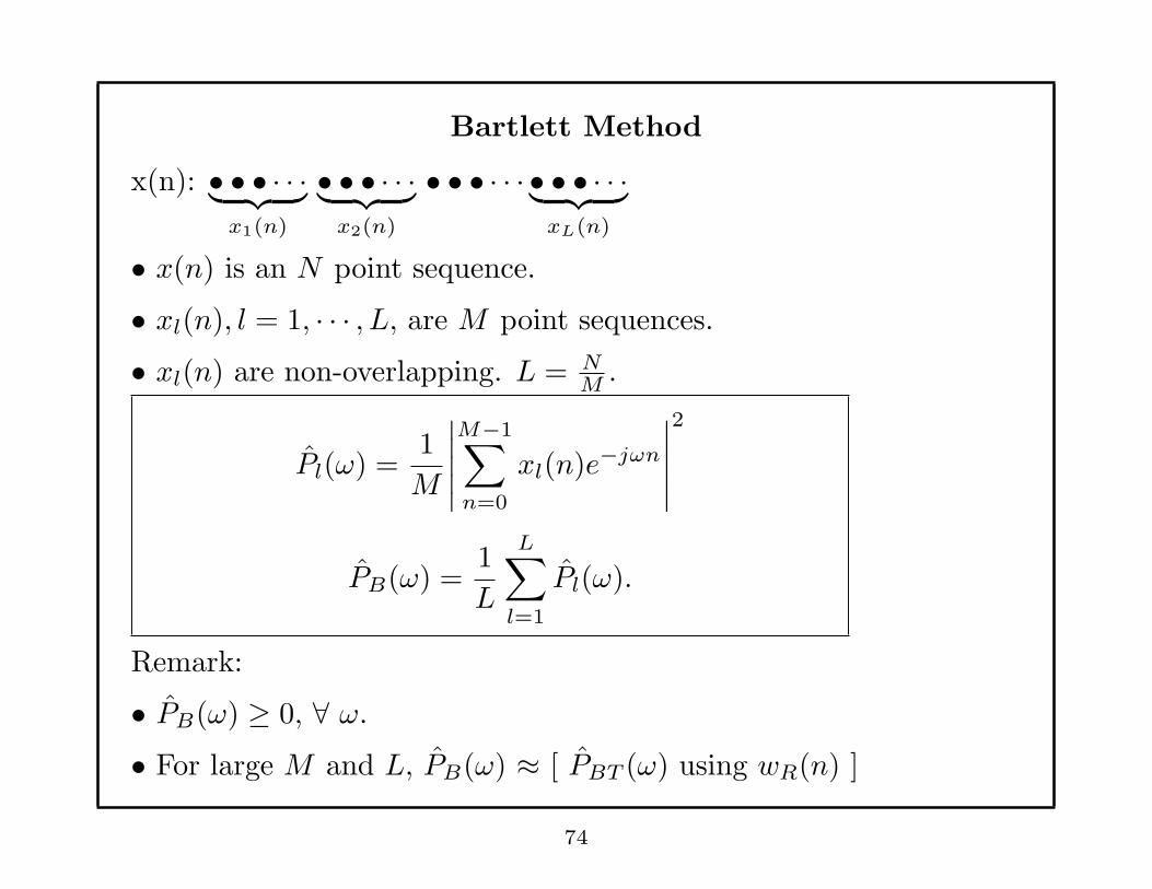
Bartlett Method
x(n): • • • · · ·︸ ︷︷ ︸
x1(n)
• • • · · ·︸ ︷︷ ︸
x2(n)
• • • · · · • • • · · ·︸ ︷︷ ︸
xL(n)
• x(n) is an N point sequence.
• xl(n), l = 1, · · · , L, are M point sequences.
• xl(n) are non-overlapping. L = NM.
Pl(ω) =1
M
∣∣∣∣∣
M−1∑
n=0
xl(n)e−jωn
∣∣∣∣∣
2
PB(ω) =1
L
L∑
l=1
Pl(ω).
Remark:
• PB(ω) ≥ 0, ∀ ω.
• For large M and L, PB(ω) ≈ [ PBT (ω) using wR(n) ]
74

Welch Method:
• xl(n) may overlap in the Welch method.
• xl(n) may be windowed before computing Periodogram.
xs (n)
x
x
1
2
(n)
(n)
Let w(n) be the window applied to xl(n), l = 1, .., S, n = 0, ..,M−1
Let
P = power of w(n) =1
M
M−1∑
n=0
|w(n)|2
75
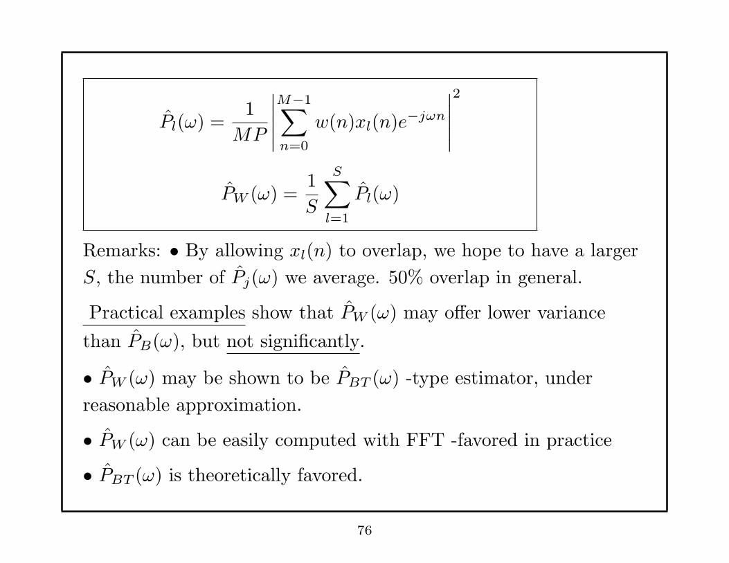
Pl(ω) =1
MP
∣∣∣∣∣
M−1∑
n=0
w(n)xl(n)e−jωn
∣∣∣∣∣
2
PW (ω) =1
S
S∑
l=1
Pl(ω)
Remarks: • By allowing xl(n) to overlap, we hope to have a larger
S, the number of Pj(ω) we average. 50% overlap in general.
Practical examples show that PW (ω) may offer lower variance
than PB(ω), but not significantly.
• PW (ω) may be shown to be PBT (ω) -type estimator, under
reasonable approximation.
• PW (ω) can be easily computed with FFT -favored in practice
• PBT (ω) is theoretically favored.
76

Daniell Method:
PD(ω) = 12πβ
∫ ω+βπ
ω−βπPp(ψ)dψ.
pP
ω−βπ ω+βπ
(ψ)
ψ
Remark: • PD(ω) is a special case of PBT (ω) with
w(n) in PBT (ω)DTFT←→ W (ω) =
1β, ω ∈ [−βπ, βπ]
0, else .
• The larger the β, the lower the variance, but the poorer the
resolution.
77

Implementation of PD(ω)
• Zero pad x(n) so that x(n) has N ′ points, N ′ >> N.
• Calculate Pp(ωk) with FFT.
ωk =2π
N ′ k, k = 0, · · · , N ′ − 1.
•
PD(ωk) =1
2J + 1
k+J∑
j=k−J
Pp(ωj).
Pp(ω) • • • · · · • • · · ·︸ ︷︷ ︸
2J+1 points averaging
•
⇓PD(ωk)
78
PARAMETRIC METHODS
Parametric Modeling
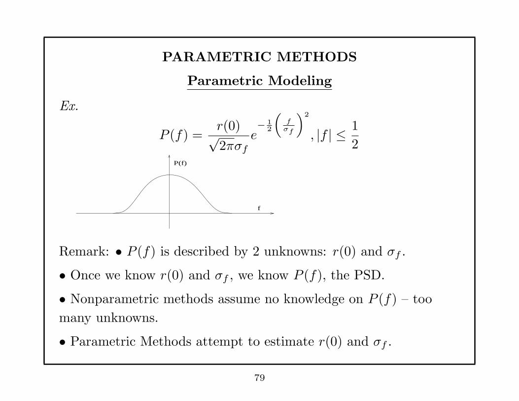
Ex.
P (f) =r(0)√2πσf
e− 1
2
(f
σf
)2
, |f | ≤ 1
2P(f)
f
Remark: • P (f) is described by 2 unknowns: r(0) and σf .
• Once we know r(0) and σf , we know P (f), the PSD.
• Nonparametric methods assume no knowledge on P (f) – too
many unknowns.
• Parametric Methods attempt to estimate r(0) and σf .
79
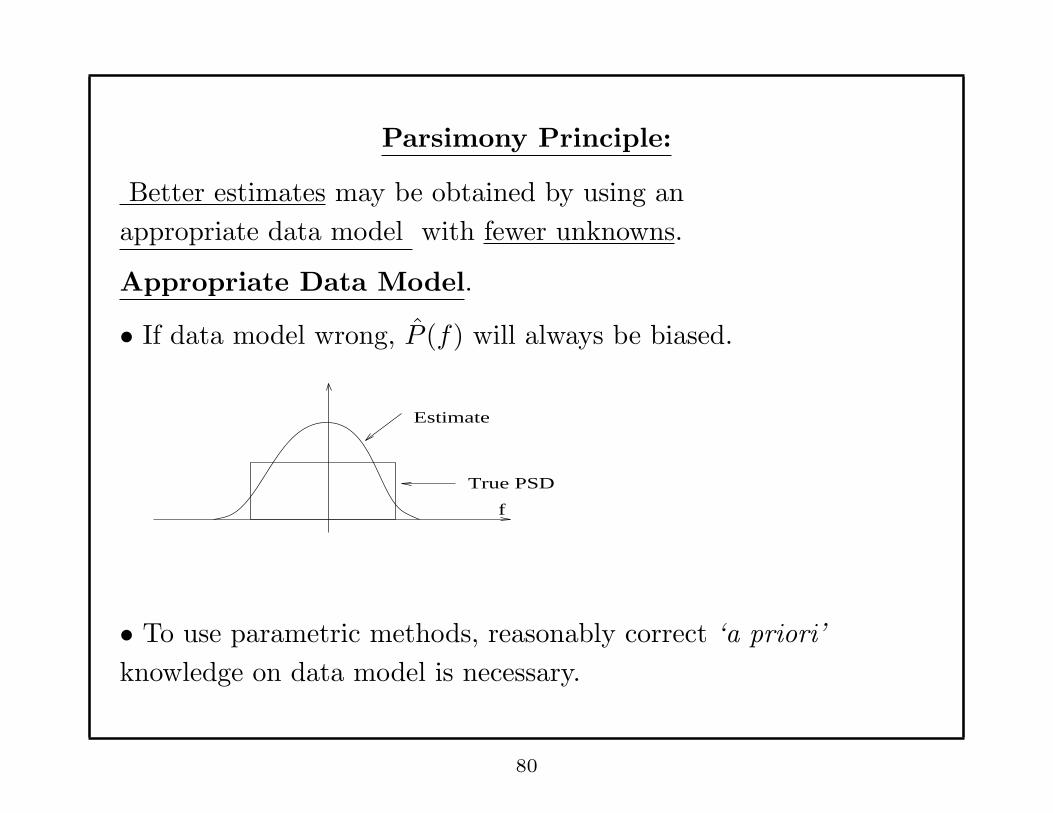
Parsimony Principle:
Better estimates may be obtained by using an
appropriate data model with fewer unknowns.
Appropriate Data Model.
• If data model wrong, P (f) will always be biased.
Estimate
True PSD
f
• To use parametric methods, reasonably correct ‘a priori’
knowledge on data model is necessary.
80
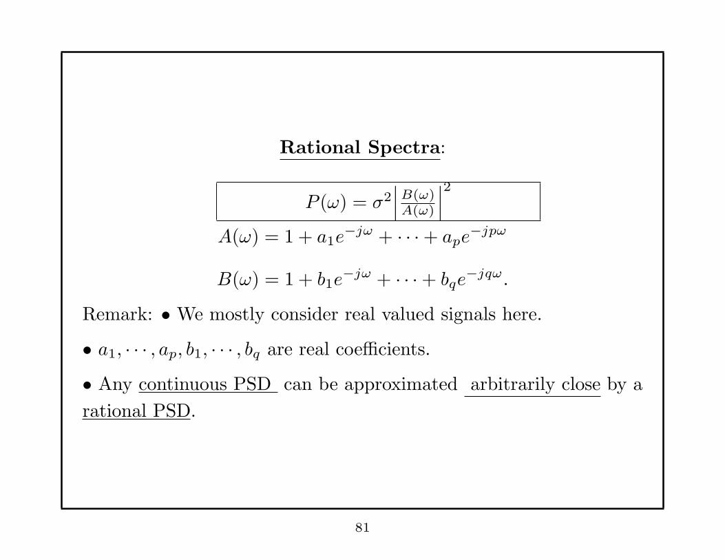
Rational Spectra:
P (ω) = σ2∣∣∣B(ω)A(ω)
∣∣∣
2
A(ω) = 1 + a1e−jω + · · ·+ ape
−jpω
B(ω) = 1 + b1e−jω + · · ·+ bqe
−jqω.
Remark: • We mostly consider real valued signals here.
• a1, · · · , ap, b1, · · · , bq are real coefficients.
• Any continuous PSD can be approximated arbitrarily close by a
rational PSD.
81
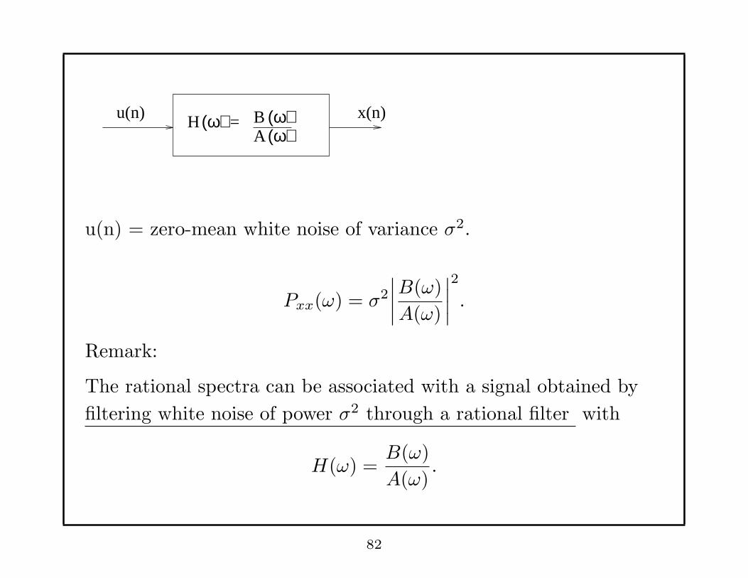
u(n) H (ω) = (ω)(ω)
x(n)BA
u(n) = zero-mean white noise of variance σ2.
Pxx(ω) = σ2
∣∣∣∣
B(ω)
A(ω)
∣∣∣∣
2
.
Remark:
The rational spectra can be associated with a signal obtained by
filtering white noise of power σ2 through a rational filter with
H(ω) =B(ω)
A(ω).
82
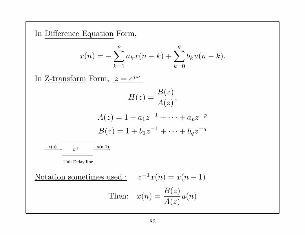
In Difference Equation Form,
x(n) = −p∑
k=1
akx(n− k) +
q∑
k=0
bku(n− k).
In Z-transform Form, z = ejω
H(z) =B(z)
A(z),
A(z) = 1 + a1z−1 + · · ·+ apz
−p
B(z) = 1 + b1z−1 + · · ·+ bqz
−q
-1z x(n) x(n-1)
Unit Delay line
Notation sometimes used : z−1x(n) = x(n− 1)
Then: x(n) =B(z)
A(z)u(n)
83
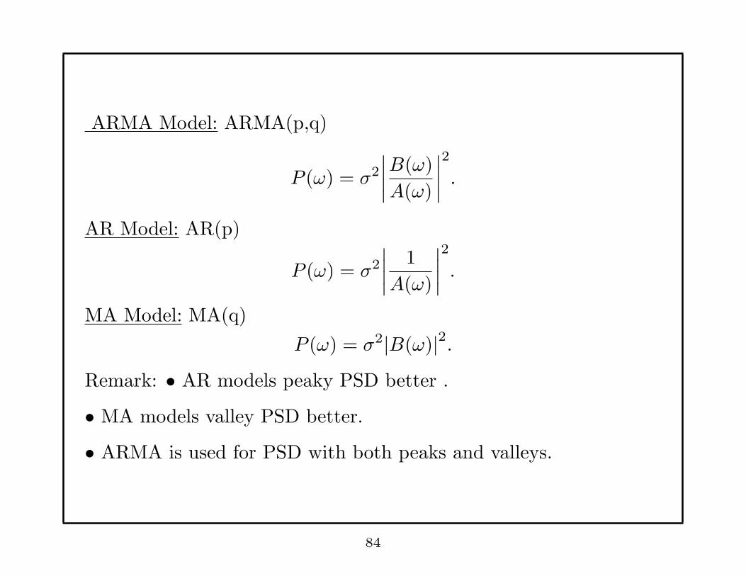
ARMA Model: ARMA(p,q)
P (ω) = σ2
∣∣∣∣
B(ω)
A(ω)
∣∣∣∣
2
.
AR Model: AR(p)
P (ω) = σ2
∣∣∣∣
1
A(ω)
∣∣∣∣
2
.
MA Model: MA(q)
P (ω) = σ2|B(ω)|2.Remark: • AR models peaky PSD better .
• MA models valley PSD better.
• ARMA is used for PSD with both peaks and valleys.
84
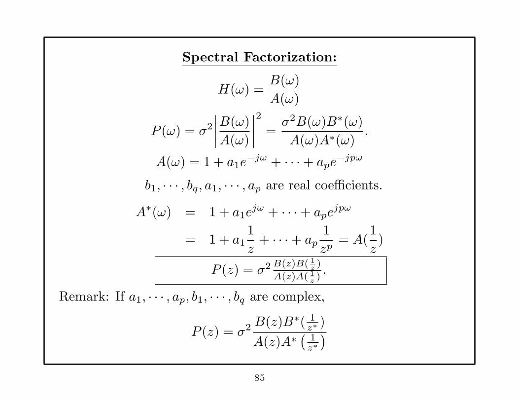
Spectral Factorization:
H(ω) =B(ω)
A(ω)
P (ω) = σ2
∣∣∣∣
B(ω)
A(ω)
∣∣∣∣
2
=σ2B(ω)B∗(ω)
A(ω)A∗(ω).
A(ω) = 1 + a1e−jω + · · ·+ ape
−jpω
b1, · · · , bq, a1, · · · , ap are real coefficients.
A∗(ω) = 1 + a1ejω + · · ·+ ape
jpω
= 1 + a11
z+ · · ·+ ap
1
zp= A(
1
z)
P (z) = σ2 B(z)B( 1z)
A(z)A( 1z).
Remark: If a1, · · · , ap, b1, · · · , bq are complex,
P (z) = σ2 B(z)B∗( 1z∗
)
A(z)A∗ ( 1z∗
)
85

Consider
P (z) = σ2B(z)B( 1z)
A(z)A( 1z).
Remark: • If α is zero for P (z), so is 1α.
• If β is a pole for P (z), so is 1β.
• Since the a1, · · · , ap, b1, · · · , bq are real, the poles and zeroes of
P (z) occur in complex conjugate pairs.
Im
Re1x x
86
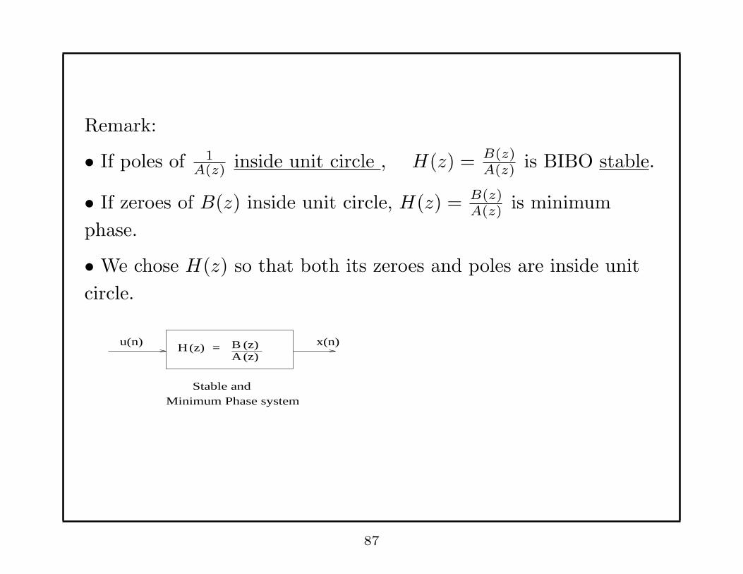
Remark:
• If poles of 1A(z) inside unit circle , H(z) = B(z)
A(z) is BIBO stable.
• If zeroes of B(z) inside unit circle, H(z) = B(z)A(z) is minimum
phase.
• We chose H(z) so that both its zeroes and poles are inside unit
circle.
u(n) H = x(n)BA
(z)(z)(z)
Minimum Phase system Stable and
87
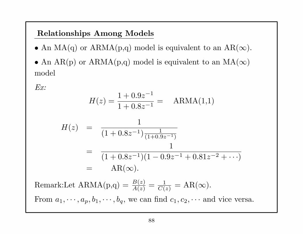
Relationships Among Models
• An MA(q) or ARMA(p,q) model is equivalent to an AR(∞).
• An AR(p) or ARMA(p,q) model is equivalent to an MA(∞)
model
Ex:
H(z) =1 + 0.9z−1
1 + 0.8z−1= ARMA(1,1)
H(z) =1
(1 + 0.8z−1) 1(1+0.9z−1)
=1
(1 + 0.8z−1)(1− 0.9z−1 + 0.81z−2 + · · ·)= AR(∞).
Remark:Let ARMA(p,q) = B(z)A(z) = 1
C(z) = AR(∞).
From a1, · · · , ap, b1, · · · , bq, we can find c1, c2, · · · and vice versa.
88
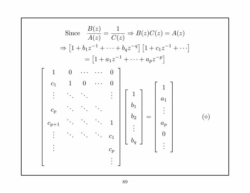
SinceB(z)
A(z)=
1
C(z)⇒ B(z)C(z) = A(z)
⇒[1 + b1z
−1 + · · ·+ bqz−q] [
1 + c1z−1 + · · ·
]
=[1 + a1z
−1 + · · ·+ apz−p]
1 0 · · · · · · 0
c1 1 0 · · · 0...
. . .. . .
...
cp. . .
. . .. . .
cp+1. . .
. . .. . . 1
.... . .
. . .. . . c1
... cp...
1
b1
b2...
bq
=
1
a1
...
ap
0...
(⋄)
89
cp+1 cp · · · cp−q+1
.... . .
. . ....
cp+q
. . . cp
1
b1...
bq
=
0
0...
0
⇒
cp · · · cp−q+1
.... . .
cp+q−1 · · · cp
b1...
bq
= −
cp+1
...
cp+q
.(∗)
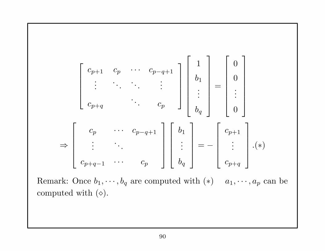
Remark: Once b1, · · · , bq are computed with (∗) a1, · · · , ap can be
computed with (⋄).
90
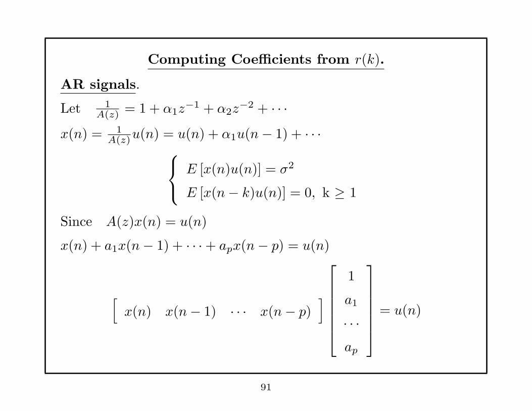
Computing Coefficients from r(k).
AR signals.
Let 1A(z) = 1 + α1z
−1 + α2z−2 + · · ·
x(n) = 1A(z)u(n) = u(n) + α1u(n− 1) + · · ·
E [x(n)u(n)] = σ2
E [x(n− k)u(n)] = 0, k ≥ 1
Since A(z)x(n) = u(n)
x(n) + a1x(n− 1) + · · ·+ apx(n− p) = u(n)
[
x(n) x(n− 1) · · · x(n− p)]
1
a1
· · ·ap
= u(n)
91
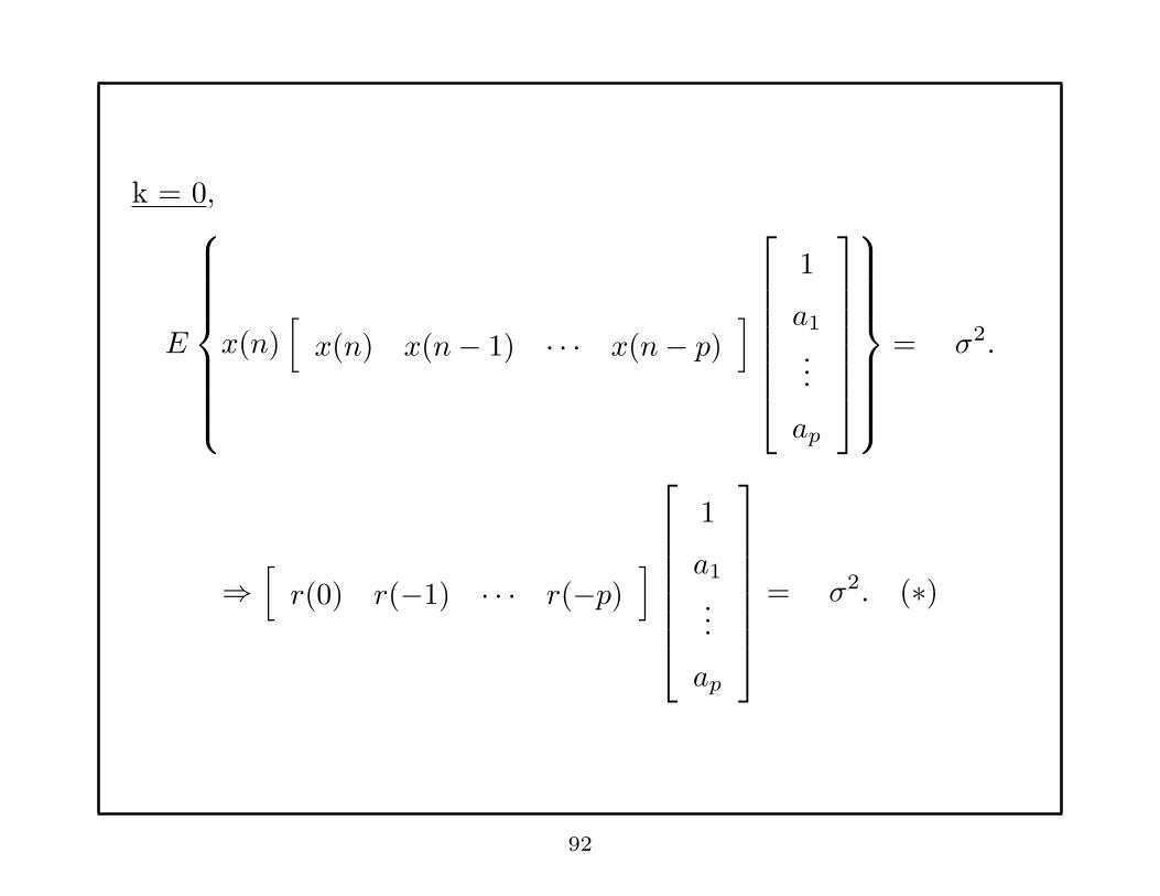
k = 0,
E
x(n)[
x(n) x(n− 1) · · · x(n− p)]
1
a1
...
ap
= σ2.
⇒[
r(0) r(−1) · · · r(−p)]
1
a1
...
ap
= σ2. (∗)
92
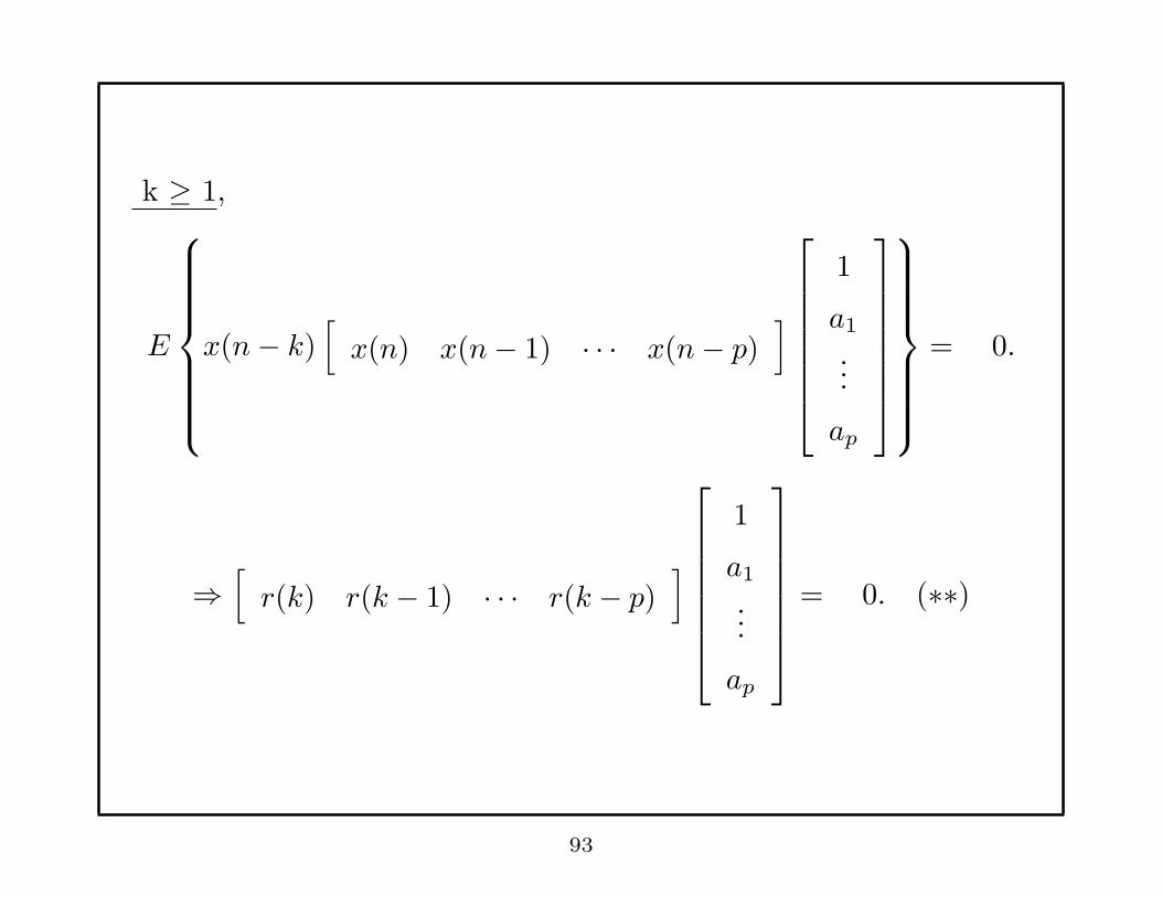
k ≥ 1,
E
x(n− k)[
x(n) x(n− 1) · · · x(n− p)]
1
a1
...
ap
= 0.
⇒[
r(k) r(k − 1) · · · r(k − p)]
1
a1
...
ap
= 0. (∗∗)
93
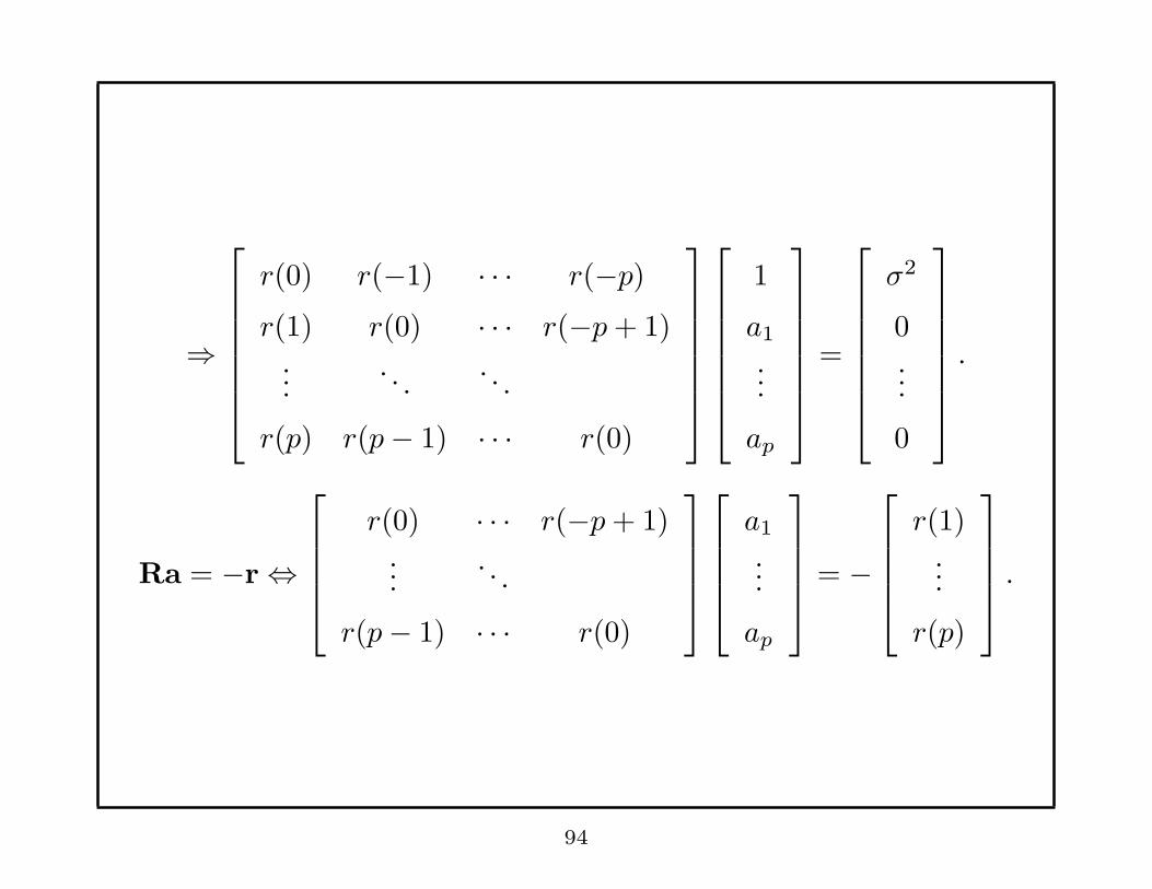
⇒
r(0) r(−1) · · · r(−p)r(1) r(0) · · · r(−p+ 1)
.... . .
. . .
r(p) r(p− 1) · · · r(0)
1
a1
...
ap
=
σ2
0...
0
.
Ra = −r⇔
r(0) · · · r(−p+ 1)...
. . .
r(p− 1) · · · r(0)
a1
...
ap
= −
r(1)...
r(p)
.
94

Remarks:
• When we only have N samples, {r(k)} is not available. {r(k)}may be used to replace {r(k)} to obtain a1, · · · , ap.
⇒ This is the Yule - Walker Method.
• R is a positive semidefinite matrix. R is positive definite unless
x(n) is a sum of less than ⌊p2⌋ sinusoids.
• R is Toeplitz.
• Levinson - Durbin algorithm is used to solve for a efficiently
• AR models are most frequently used in practice.
• Estimation of AR parameters is a well-established topic.
95
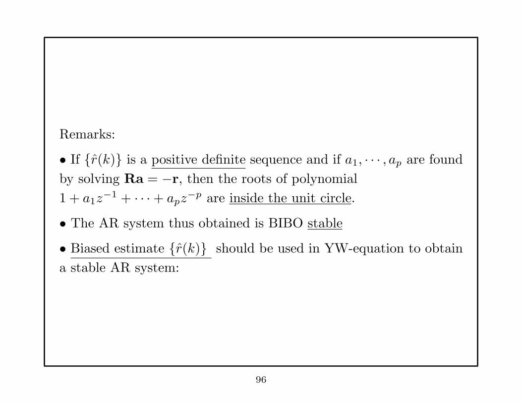
Remarks:
• If {r(k)} is a positive definite sequence and if a1, · · · , ap are found
by solving Ra = −r, then the roots of polynomial
1 + a1z−1 + · · ·+ apz
−p are inside the unit circle.
• The AR system thus obtained is BIBO stable
• Biased estimate {r(k)} should be used in YW-equation to obtain
a stable AR system:
96

Efficient Methods for solving
Ra = −r or Ra = −r
• Levinson - Durbin Algorithm.
• Delsarte - Genin Algorithm.
• Gohberg - Semencul Formula for R−1 or R−1
(Sometimes, we may be interested in not only a but also R−1 )
97
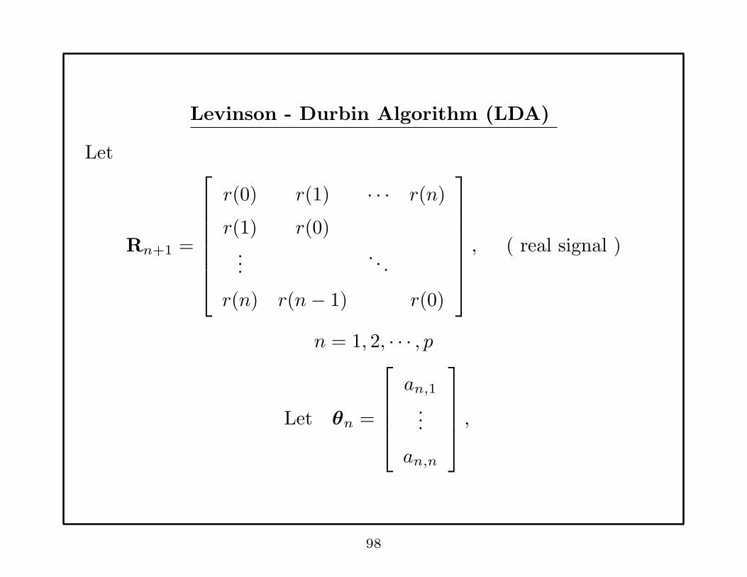
Levinson - Durbin Algorithm (LDA)
Let
Rn+1 =
r(0) r(1) · · · r(n)
r(1) r(0)...
. . .
r(n) r(n− 1) r(0)
, ( real signal )
n = 1, 2, · · · , p
Let θn =
an,1
...
an,n
,
98
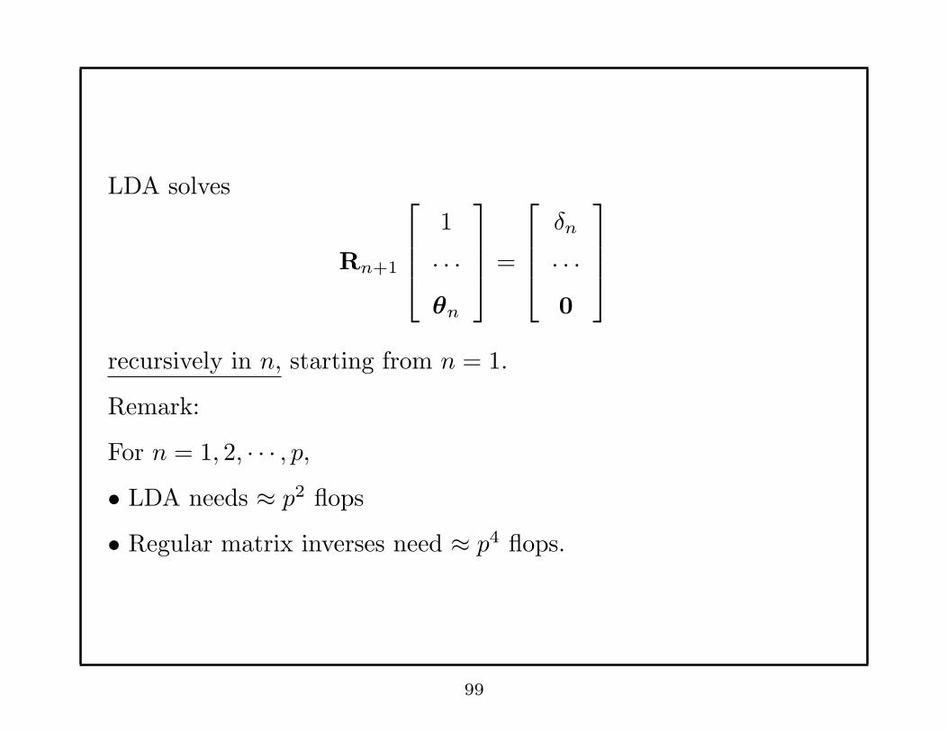
LDA solves
Rn+1
1
· · ·θn
=
δn
· · ·0
recursively in n, starting from n = 1.
Remark:
For n = 1, 2, · · · , p,• LDA needs ≈ p2 flops
• Regular matrix inverses need ≈ p4 flops.
99
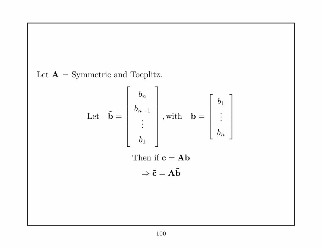
Let A = Symmetric and Toeplitz.
Let b =
bn
bn−1
...
b1
,with b =
b1...
bn
Then if c = Ab
⇒ c = Ab
100
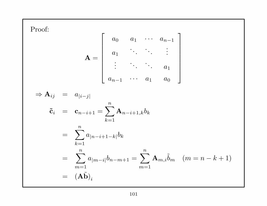
Proof:
A =
a0 a1 · · · an−1
a1. . .
. . ....
.... . .
. . . a1
an−1 · · · a1 a0
⇒ Aij = a|i−j|
ci = cn−i+1 =n∑
k=1
An−i+1,kbk
=n∑
k=1
a|n−i+1−k|bk
=n∑
m=1
a|m−i|bn−m+1 =n∑
m=1
Am,ibm (m = n− k + 1)
= (Ab)i
101
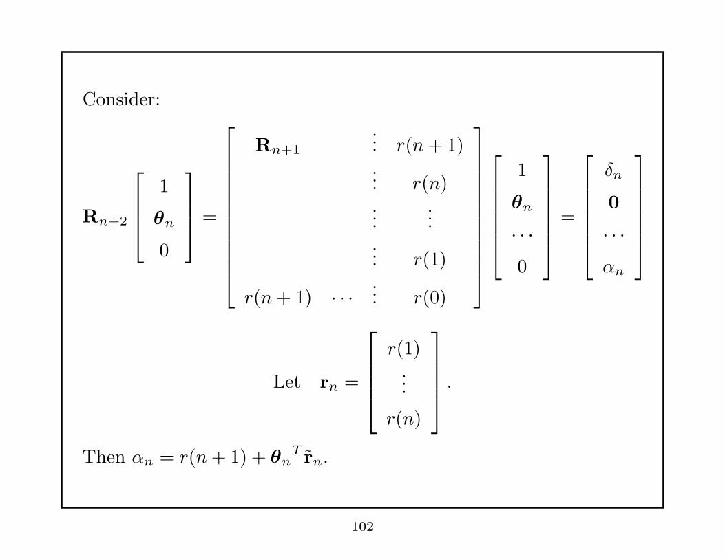
Consider:
Rn+2
1
θn
0
=
Rn+1
... r(n+ 1)
... r(n)
......
... r(1)
r(n+ 1) · · ·... r(0)
1
θn
· · ·0
=
δn
0
· · ·αn
Let rn =
r(1)...
r(n)
.
Then αn = r(n+ 1) + θnT rn.
102
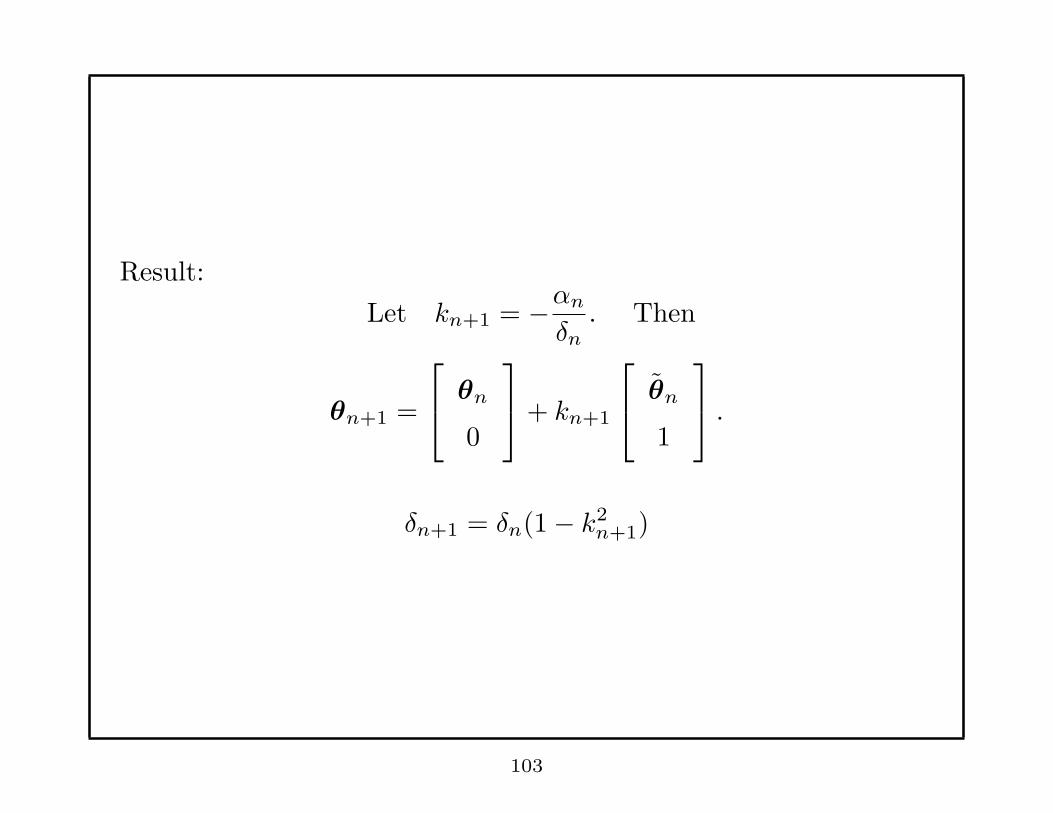
Result:
Let kn+1 = −αn
δn. Then
θn+1 =
θn
0
+ kn+1
θn
1
.
δn+1 = δn(1− k2n+1)
103
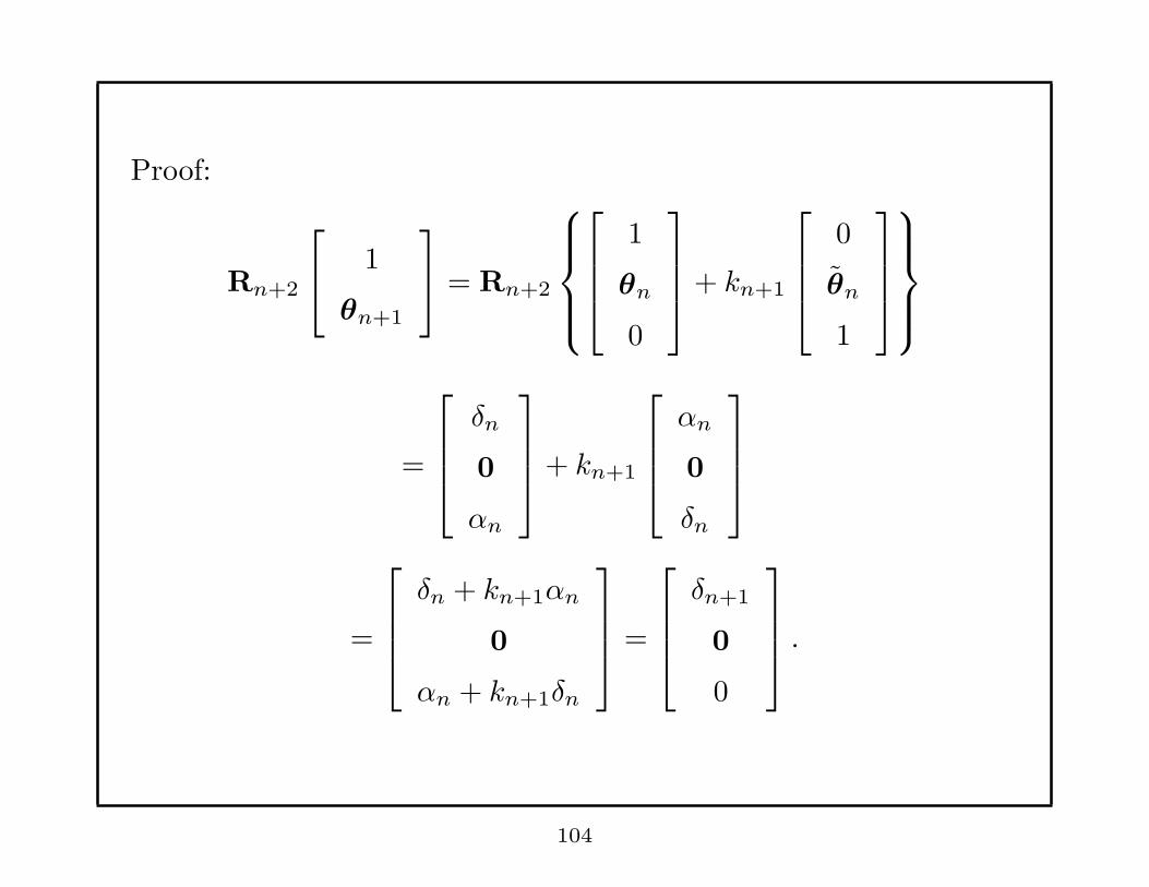
Proof:
Rn+2
1
θn+1
= Rn+2
1
θn
0
+ kn+1
0
θn
1
=
δn
0
αn
+ kn+1
αn
0
δn
=
δn + kn+1αn
0
αn + kn+1δn
=
δn+1
0
0
.
104
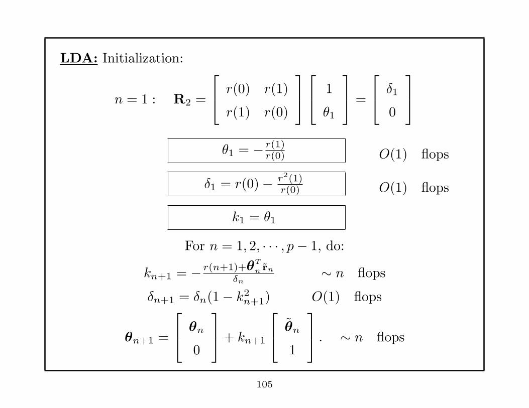
LDA: Initialization:
n = 1 : R2 =
r(0) r(1)
r(1) r(0)
1
θ1
=
δ1
0
θ1 = − r(1)r(0) O(1) flops
δ1 = r(0)− r2(1)r(0) O(1) flops
k1 = θ1
For n = 1, 2, · · · , p− 1, do:
kn+1 = − r(n+1)+θT
n rn
δn∼ n flops
δn+1 = δn(1− k2n+1) O(1) flops
θn+1 =
θn
0
+ kn+1
θn
1
. ∼ n flops
105

Ex:
1 ρ ρ2
ρ 1 ρ
ρ2 ρ 1
1
a1
a2
=
σ2
0
0
.
Straightforward Solution:
a1
a2
= −
1 ρ
ρ 1
−1
ρ
ρ2
= − 1
(1− ρ2)
1 −ρ−ρ 1
ρ
ρ2
=
−ρ0
⇒ σ2 = 1− ρ2.
106

LDA: Initialization:
θ1 = − r(1)r(0) = −ρ
1 = −ρδ1 = r(0)− r2(1)
r(0) = 1− ρ2.
k1 = θ1 = −ρ.
r1 = ρ,
k2 = −r(2) + θT1 r1
δ1
= −ρ2 + (−ρ)ρ1− ρ2
= 0
δ2 = δ1(1− k22) = (1− ρ2)(1− 02)
= 1− ρ2 = σ2
107

θ2 =
θ1
0
+ k2
θ1
1
=
−ρ0
+ 0
−ρ1
=
−ρ0
=
a1
a2
Properties of LDA:
• |kn| < 1, n = 1, 2, · · · , p, and r(0) > 0, iff
An(z) = 1 + an,1z−1 + · · ·+ an,nz
−n = 0
has roots inside the unit circle.
• |kn| < 1, n = 1, 2, · · · , p, and r(0) > 0 iff Rn+1 > 0
108
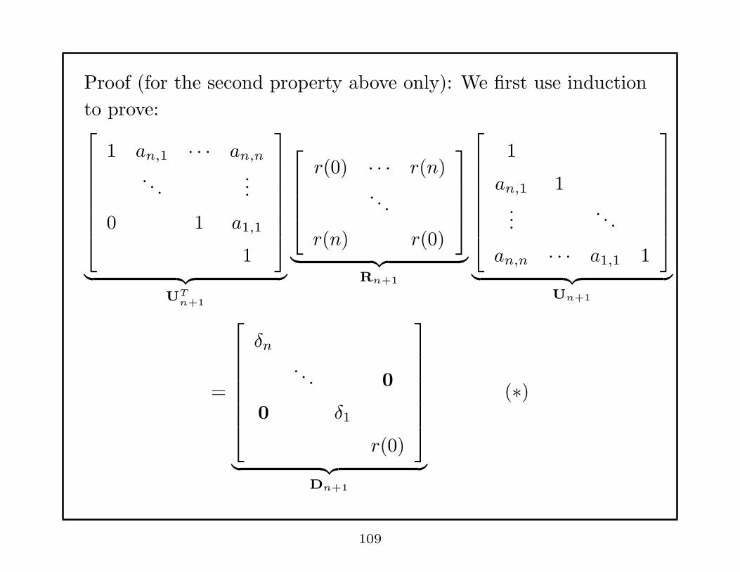
Proof (for the second property above only): We first use induction
to prove:
1 an,1 · · · an,n
. . ....
0 1 a1,1
1
︸ ︷︷ ︸
UTn+1
r(0) · · · r(n)
. . .
r(n) r(0)
︸ ︷︷ ︸
Rn+1
1
an,1 1...
. . .
an,n · · · a1,1 1
︸ ︷︷ ︸
Un+1
=
δn
. . . 0
0 δ1
r(0)
︸ ︷︷ ︸
Dn+1
(∗)
109
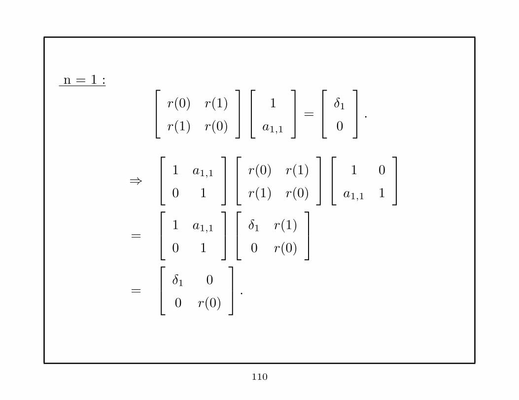
n = 1 :
r(0) r(1)
r(1) r(0)
1
a1,1
=
δ1
0
.
⇒
1 a1,1
0 1
r(0) r(1)
r(1) r(0)
1 0
a1,1 1
=
1 a1,1
0 1
δ1 r(1)
0 r(0)
=
δ1 0
0 r(0)
.
110

Suppose (∗) is true for n = k − 1, i.e.,
UTk RkUk = Dk.
Consider n = k:
UTk+1Rk+1Uk+1 =
1 θT
k
0 UTk
r(0) rT
k
rk Rk
1 0
θk Uk
=
r(0) + θT
k rk rTk + θT
k Rk
UTk rk UkRk
1 0
θk Uk
Since Rk+1
1
θk
=
δk
0
111

⇒
r(0) rT
k
rk Rk
1
θk
=
δk
0
⇒ r(0) + rTk θk = δk ⇒ r(0) + θT
k rk = δk
rk + Rkθk = 0 ⇒ rTk + θT
k RTk
= rTk + θT
k Rk = 0
⇒ UTk+1Rk+1Uk+1 =
δk 0
UTk rk UT
k Rk
1 0
θk Uk
=
δk 0
UTk rk + UT
k Rkθk UTk RkUk
=
δk 0
0 Dk
= Dk+1
112
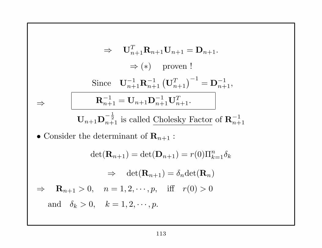
⇒ UTn+1Rn+1Un+1 = Dn+1.
⇒ (∗) proven !
Since U−1n+1R
−1n+1
(UT
n+1
)−1= D−1
n+1,
⇒ R−1n+1 = Un+1D
−1n+1U
Tn+1.
Un+1D− 1
2n+1 is called Cholesky Factor of R−1
n+1
• Consider the determinant of Rn+1 :
det(Rn+1) = det(Dn+1) = r(0)Πnk=1δk
⇒ det(Rn+1) = δndet(Rn)
⇒ Rn+1 > 0, n = 1, 2, · · · , p, iff r(0) > 0
and δk > 0, k = 1, 2, · · · , p.
113

Recall
δn+1 = δn(1− k2n+1).
If Rn+1 > 0,
⇒ r(0) > 0, δn > 0, n = 1, 2, · · · , p,
k2n+1 =
δn − δn+1
δn
Since δn − δn+1 < δn,
k2n+1 < 1 ⇒ |kn+1| < 1.
If |kn| < 1, r(0) > 0,
⇒ k2n+1 < 1.
⇒
δ0 = r(0) > 0,
δn+1 = δn(1− k2n+1) > 0, n = 1, 2, · · · , p− 1
114

MA Signals:
x(n) = B(z)u(n)
= u(n) + b1u(n− 1) + · · ·+ bqu(n− q)r(k) = E [x(n)x(n− k)]
= E {[u(n) + · · ·+ bqu(n− q)][u(n− k) + · · ·+ bqu(n− q − k)]}
|k| > q : r(k) = 0
|k| < q : r(k) = σ2
q−k∑
l=0
blbl+k, q > k ≥ 0
r(k) = r(−k). − q < k < 0
b0 = 1, b1, · · · , bq = real.
⇒ P (ω) =∑q
k=−q r(k)e−jωk.
115
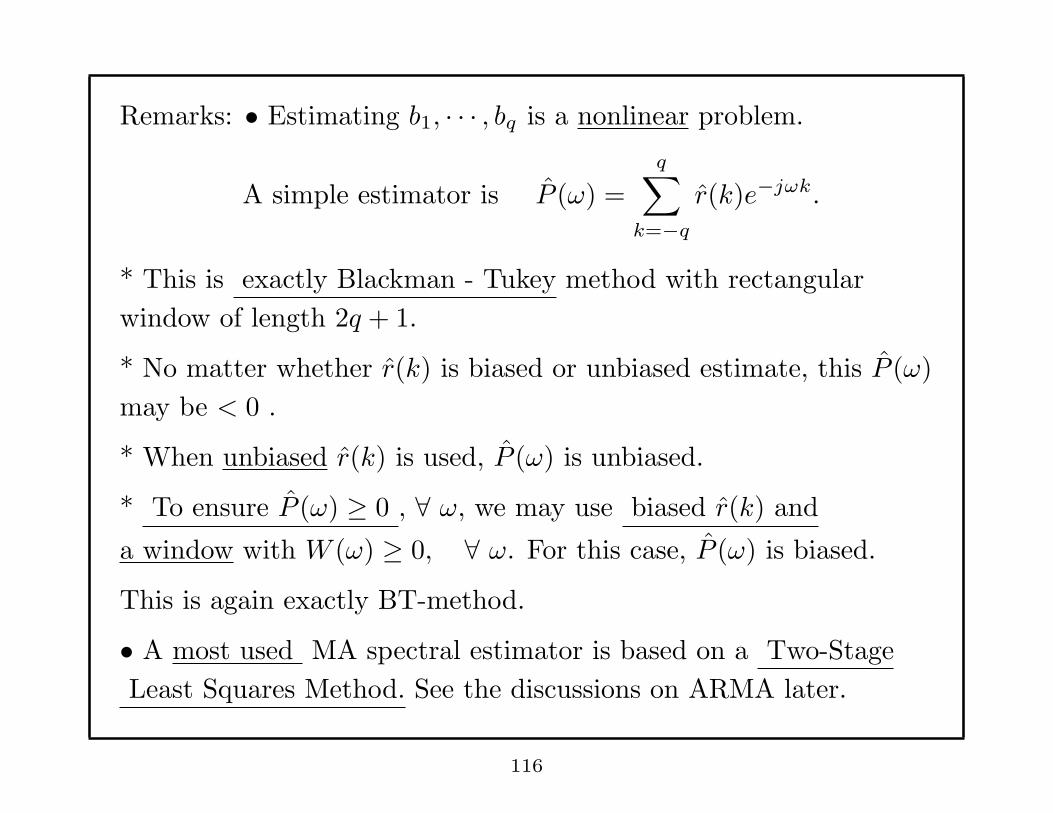
Remarks: • Estimating b1, · · · , bq is a nonlinear problem.
A simple estimator is P (ω) =
q∑
k=−q
r(k)e−jωk.
* This is exactly Blackman - Tukey method with rectangular
window of length 2q + 1.
* No matter whether r(k) is biased or unbiased estimate, this P (ω)
may be < 0 .
* When unbiased r(k) is used, P (ω) is unbiased.
* To ensure P (ω) ≥ 0 , ∀ ω, we may use biased r(k) and
a window with W (ω) ≥ 0, ∀ ω. For this case, P (ω) is biased.
This is again exactly BT-method.
• A most used MA spectral estimator is based on a Two-Stage
Least Squares Method. See the discussions on ARMA later.
116
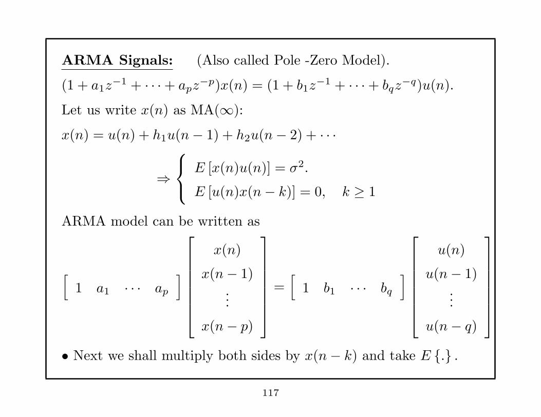
ARMA Signals: (Also called Pole -Zero Model).
(1 + a1z−1 + · · ·+ apz
−p)x(n) = (1 + b1z−1 + · · ·+ bqz
−q)u(n).
Let us write x(n) as MA(∞):
x(n) = u(n) + h1u(n− 1) + h2u(n− 2) + · · ·
⇒
E [x(n)u(n)] = σ2.
E [u(n)x(n− k)] = 0, k ≥ 1
ARMA model can be written as
[
1 a1 · · · ap
]
x(n)
x(n− 1)...
x(n− p)
=[
1 b1 · · · bq
]
u(n)
u(n− 1)...
u(n− q)
• Next we shall multiply both sides by x(n− k) and take E {.} .
117

k= 0:
[
1 a1 · · · ap
]
r(0)
r(1)...
r(p)
=[
1 b1 · · · bq
]
σ2
σ2h1
...
σ2hq
k = 1:
[
1 a1 · · · ap
]
r(−1)
r(0)...
r(p− 1)
=[
1 b1 · · · bq
]
0
σ2
σ2h1
...
σ2hq−1
...
118
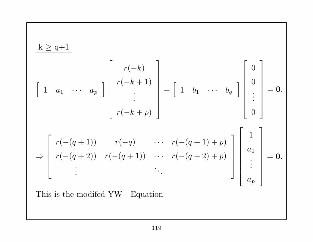
k ≥ q+1
[
1 a1 · · · ap
]
r(−k)r(−k + 1)
...
r(−k + p)
=[
1 b1 · · · bq
]
0
0...
0
= 0.
⇒
r(−(q + 1)) r(−q) · · · r(−(q + 1) + p)
r(−(q + 2)) r(−(q + 1)) · · · r(−(q + 2) + p)...
. . .
1
a1
...
ap
= 0.
This is the modifed YW - Equation
119
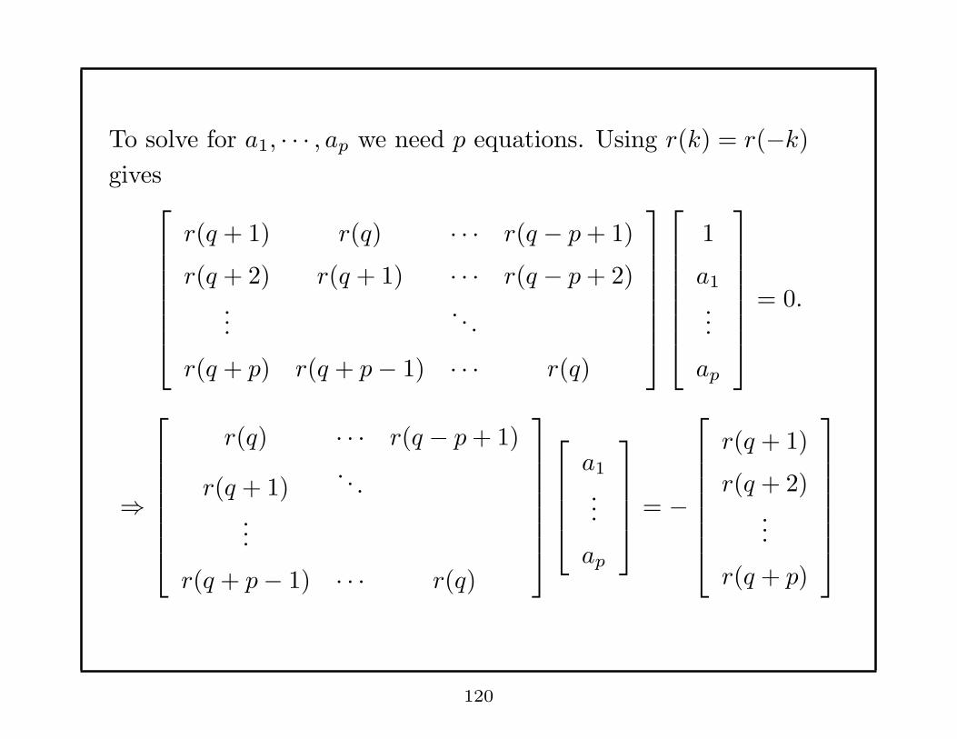
To solve for a1, · · · , ap we need p equations. Using r(k) = r(−k)gives
r(q + 1) r(q) · · · r(q − p+ 1)
r(q + 2) r(q + 1) · · · r(q − p+ 2)...
. . .
r(q + p) r(q + p− 1) · · · r(q)
1
a1
...
ap
= 0.
⇒
r(q) · · · r(q − p+ 1)
r(q + 1). . .
...
r(q + p− 1) · · · r(q)
a1
...
ap
= −
r(q + 1)
r(q + 2)...
r(q + p)
120
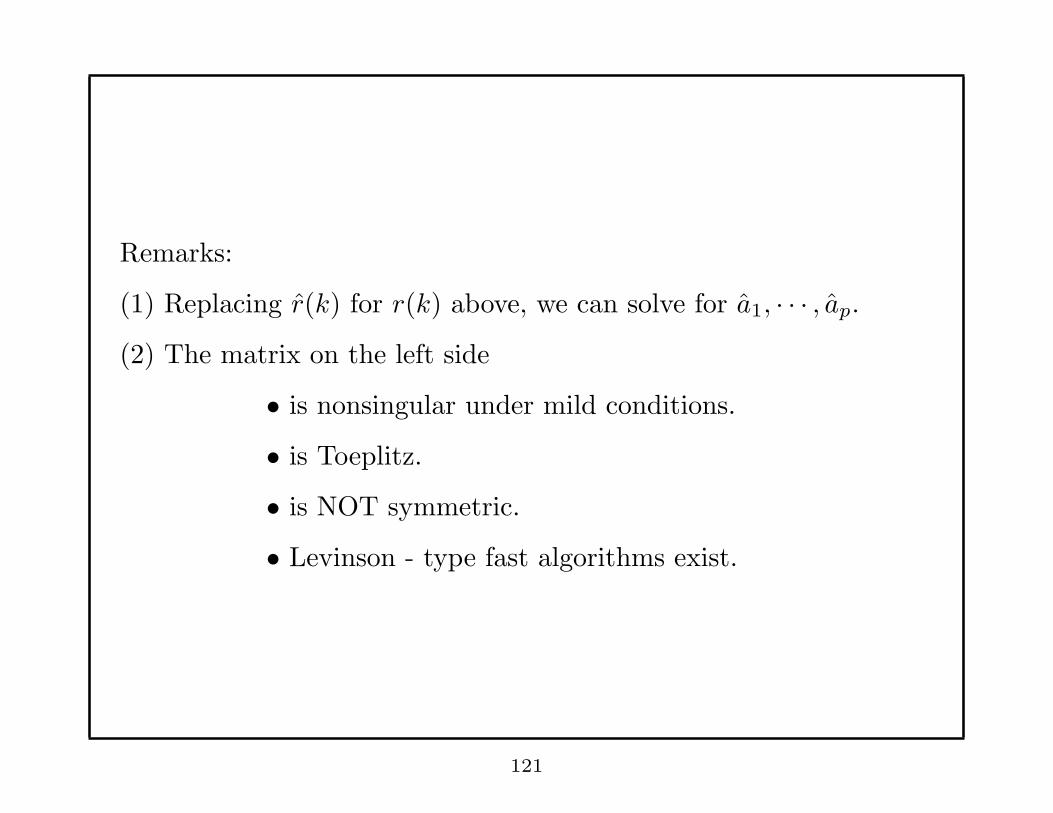
Remarks:
(1) Replacing r(k) for r(k) above, we can solve for a1, · · · , ap.
(2) The matrix on the left side
• is nonsingular under mild conditions.
• is Toeplitz.
• is NOT symmetric.
• Levinson - type fast algorithms exist.
121

What about the MA part of the ARMA PSD?
Let y(n) = (1 + b1z−1 + · · ·+ bqz
−q)u(n).
The ARMA model becomes
(1 + a1z−1 + · · ·+ apz
−p)x(n) = y(n)
y(n) x(n) x(n)A(z)
y(n),A(z)
1
Px(ω) =
∣∣∣∣
1
A(ω)
∣∣∣∣
2
Py(ω).
Let γk be the autocorrelation function of y(n) . Then (see MA
signals).
Py(ω) =
q∑
k=−q
γke−jωk
122
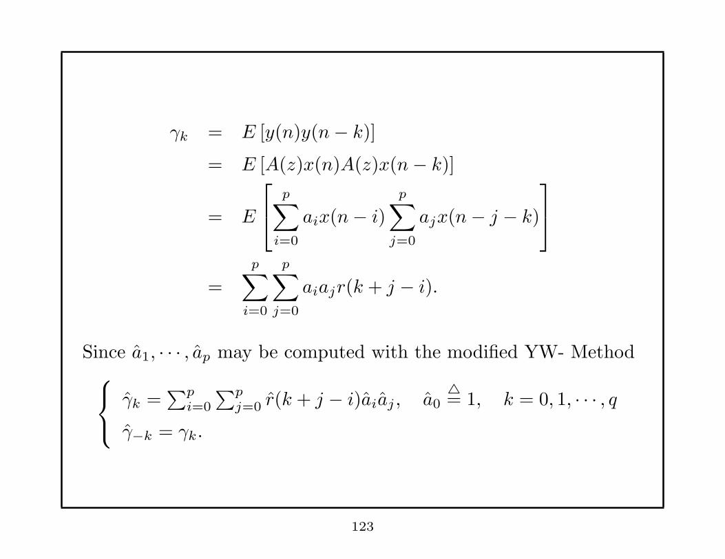
γk = E [y(n)y(n− k)]= E [A(z)x(n)A(z)x(n− k)]
= E
p∑
i=0
aix(n− i)p∑
j=0
ajx(n− j − k)
=
p∑
i=0
p∑
j=0
aiajr(k + j − i).
Since a1, · · · , ap may be computed with the modified YW- Method
γk =∑p
i=0
∑pj=0 r(k + j − i)aiaj , a0
△= 1, k = 0, 1, · · · , q
γ−k = γk.
123

ARMA PSD Estimate:
P (ω) =
∑qk=−q γke
−jωk
∣∣∣A(ω)
∣∣∣
2
Remarks:
• This method is called modified YW ARMA Spectral Estimator
• P (ω) is not guaranteed to be ≥ 0, ∀ ω, due to the MA part.
• The AR estimates a1, · · · , ap have reasonable accuracy if the
ARMA poles and zeroes are well inside the unit circle.
• Very poor estimates a1, · · · , ap occur when ARMA poles and
zeroes are closely-spaced and nearby unit circle. (This is
narrowband signal case).
124
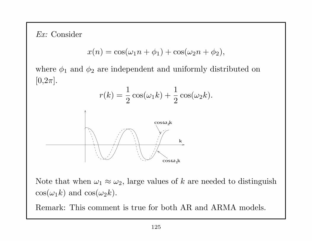
Ex: Consider
x(n) = cos(ω1n+ φ1) + cos(ω2n+ φ2),
where φ1 and φ2 are independent and uniformly distributed on
[0,2π].
r(k) =1
2cos(ω1k) +
1
2cos(ω2k).
cos
k
ω
cosω2
1
k
k
Note that when ω1 ≈ ω2, large values of k are needed to distinguish
cos(ω1k) and cos(ω2k).
Remark: This comment is true for both AR and ARMA models.
125
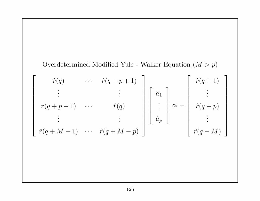
Overdetermined Modified Yule - Walker Equation (M > p)
r(q) · · · r(q − p+ 1)...
...
r(q + p− 1) · · · r(q)...
...
r(q +M − 1) · · · r(q +M − p)
a1
...
ap
≈ −
r(q + 1)...
r(q + p)...
r(q +M)
126
Remarks:
• The overdetermined linear equations may be solved with
Least Squares or Total Least Squares Methods.
• M should be chosen based on the trade-off between information
contained in the large lags of r(k) and the accuracy of r(k).
• Overdetermined YW -equation may also be obtained for AR
signals.
127
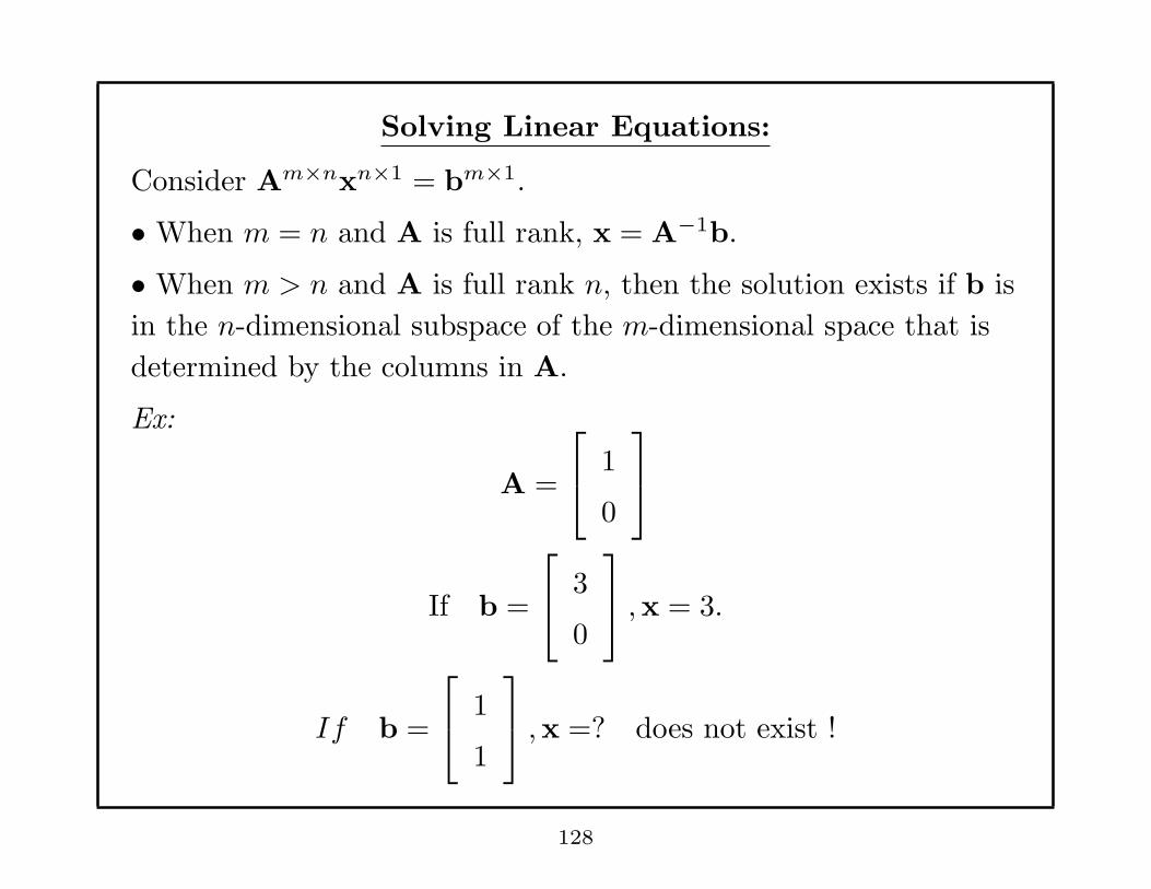
Solving Linear Equations:
Consider Am×nxn×1 = bm×1.
• When m = n and A is full rank, x = A−1b.
• When m > n and A is full rank n, then the solution exists if b is
in the n-dimensional subspace of the m-dimensional space that is
determined by the columns in A.
Ex:
A =
1
0
If b =
3
0
,x = 3.
If b =
1
1
,x =? does not exist !
128
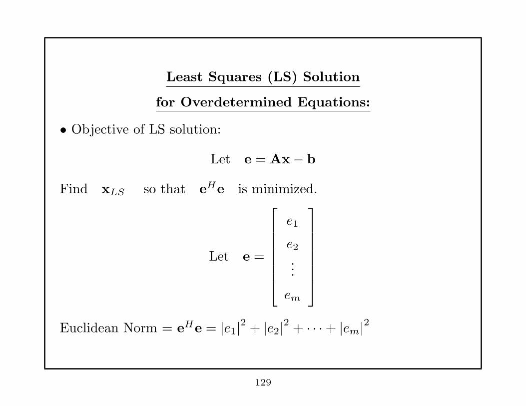
Least Squares (LS) Solution
for Overdetermined Equations:
• Objective of LS solution:
Let e = Ax− b
Find xLS so that eHe is minimized.
Let e =
e1
e2...
em
Euclidean Norm = eHe = |e1|2 + |e2|2 + · · ·+ |em|2
129

Ex:
m
2
e
e 1
e
Remarks: • AxLS = b + eLS
• We see that xLS is found by perturbing b so that a solution
exists.
130
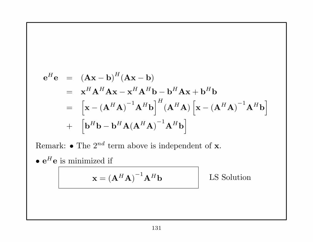
eHe = (Ax− b)H
(Ax− b)
= xHAHAx− xHAHb− bHAx + bHb
=[
x− (AHA)−1
AHb]H
(AHA)[
x− (AHA)−1
AHb]
+[
bHb− bHA(AHA)−1
AHb]
Remark: • The 2nd term above is independent of x.
• eHe is minimized if
x = (AHA)−1
AHb LS Solution
131
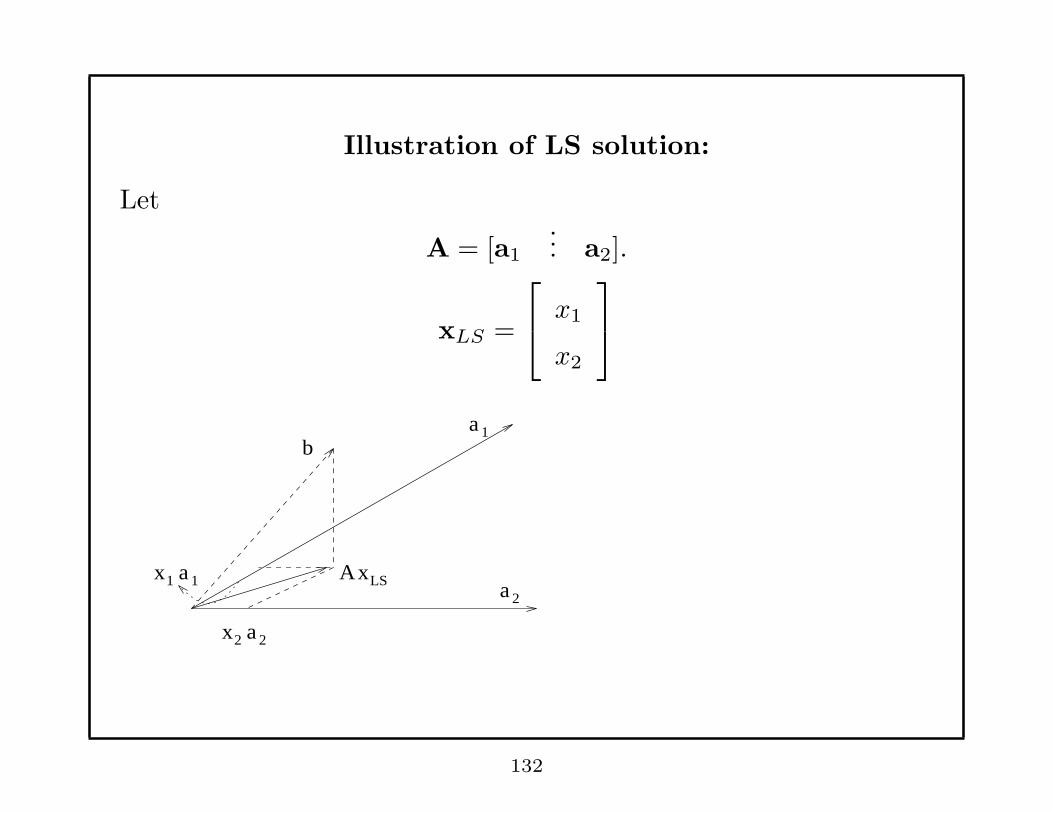
Illustration of LS solution:
Let
A = [a1
... a2].
xLS =
x1
x2
1b
a
aA
x
x1 a 1
2 a 2
xLS2
132
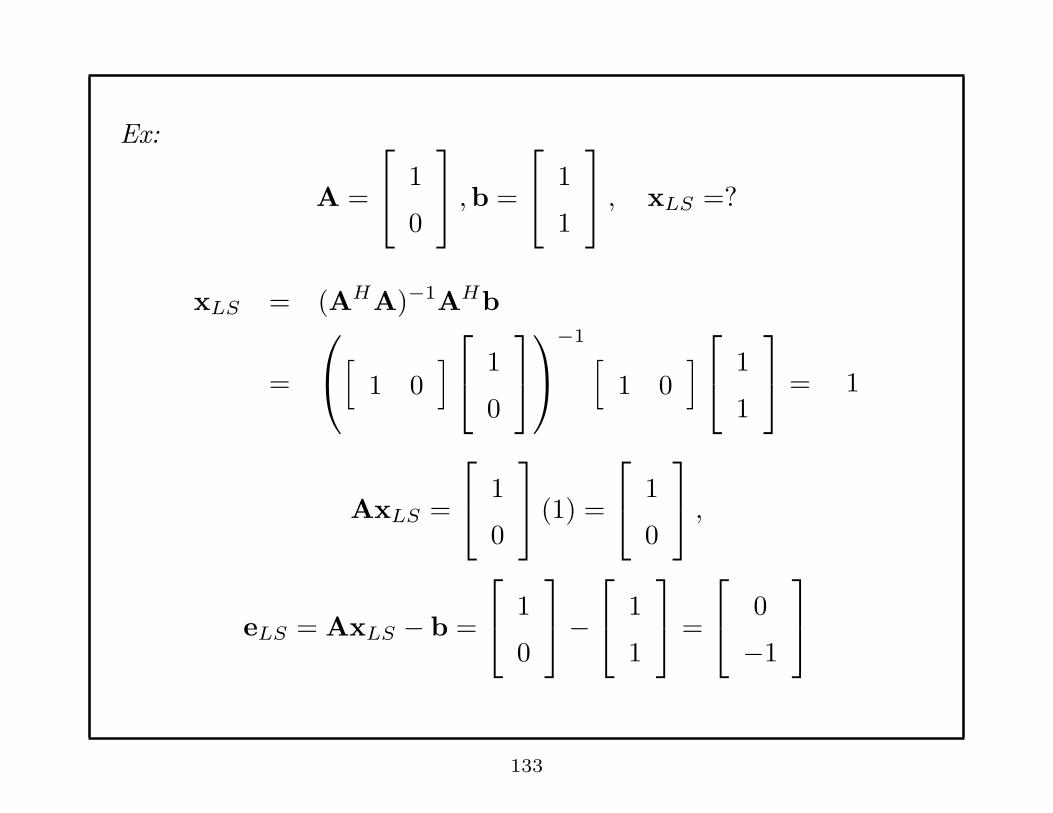
Ex:
A =
1
0
,b =
1
1
, xLS =?
xLS = (AHA)−1AHb
=
[
1 0]
1
0
−1[
1 0]
1
1
= 1
AxLS =
1
0
(1) =
1
0
,
eLS = AxLS − b =
1
0
−
1
1
=
0
−1
133
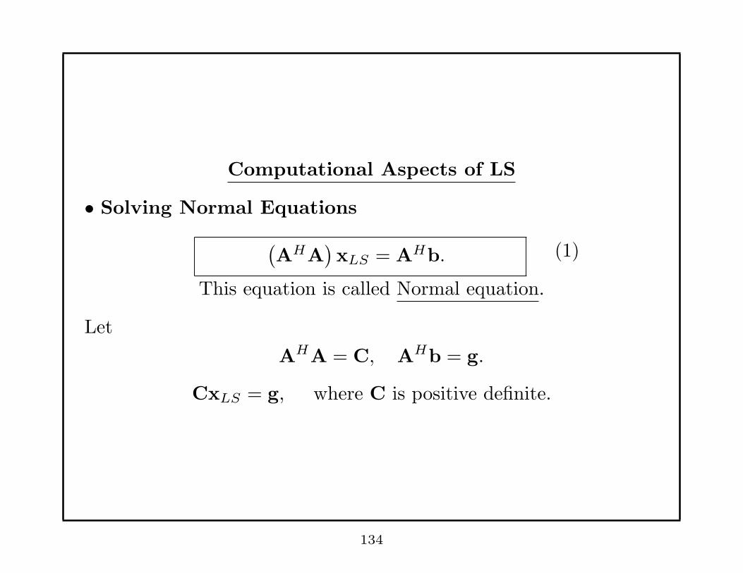
Computational Aspects of LS
• Solving Normal Equations
(AHA
)xLS = AHb. (1)
This equation is called Normal equation.
Let
AHA = C, AHb = g.
CxLS = g, where C is positive definite.
134
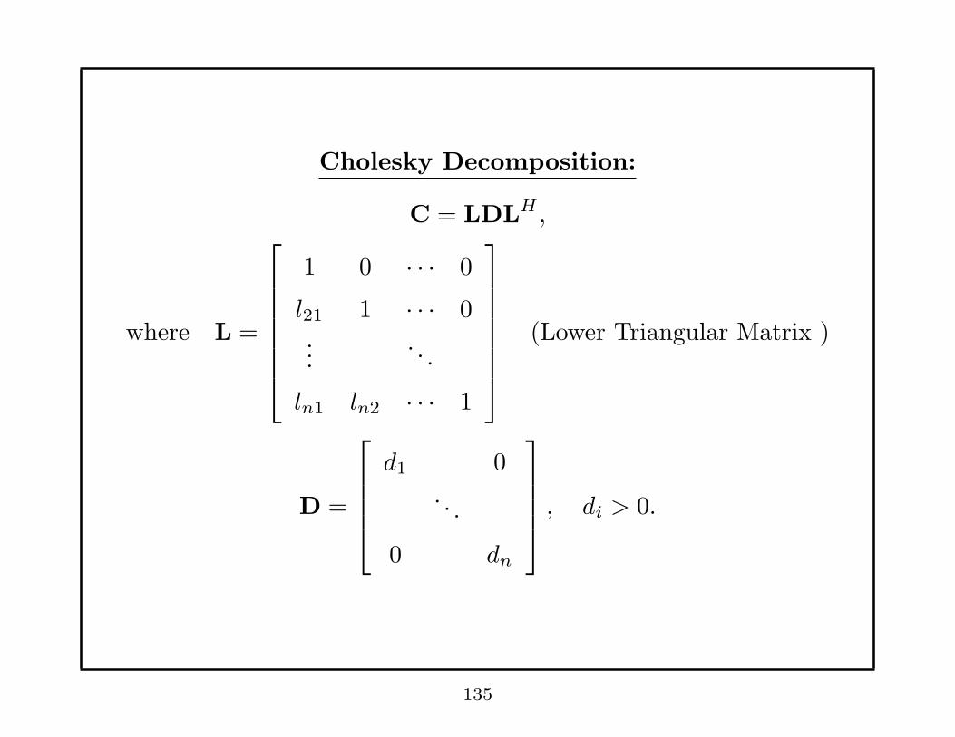
Cholesky Decomposition:
C = LDLH ,
where L =
1 0 · · · 0
l21 1 · · · 0...
. . .
ln1 ln2 · · · 1
(Lower Triangular Matrix )
D =
d1 0
. . .
0 dn
, di > 0.
135
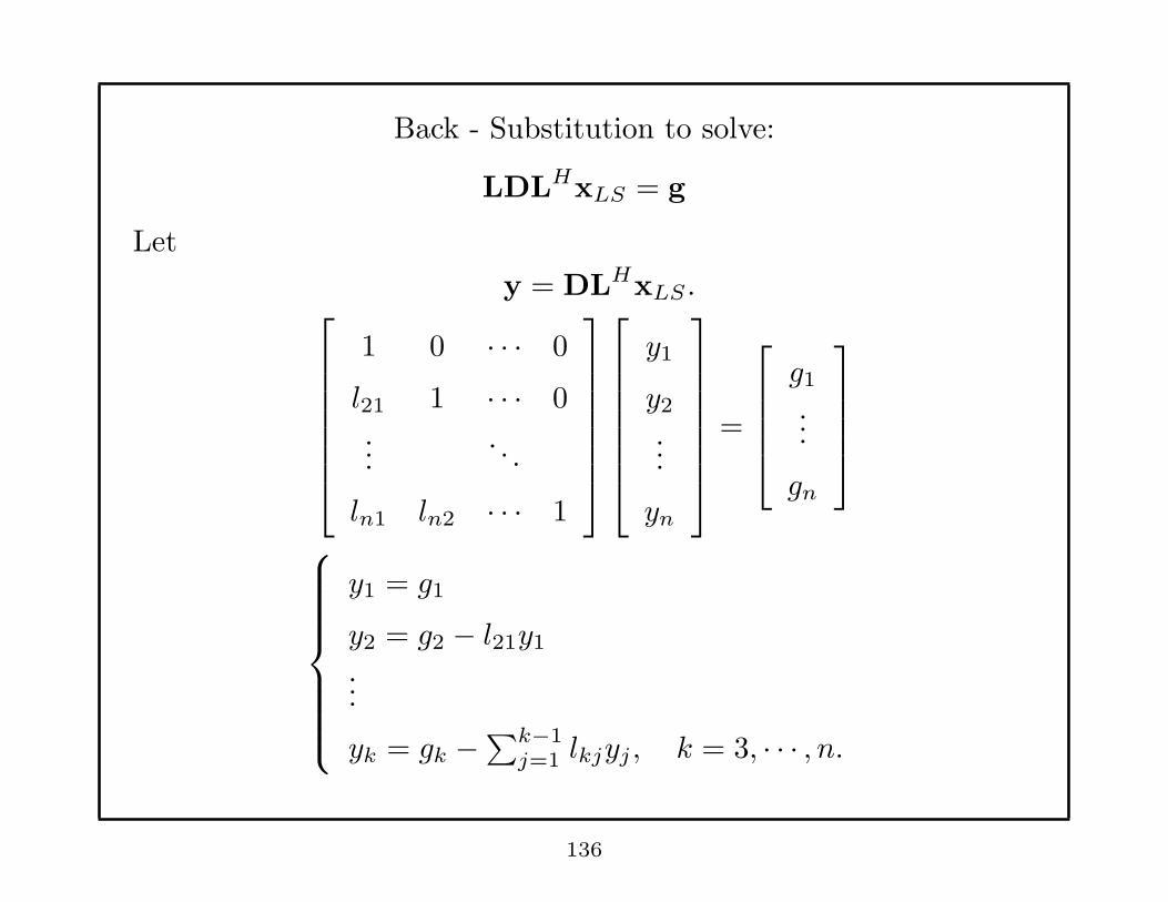
Back - Substitution to solve:
LDLHxLS = g
Let
y = DLHxLS .
1 0 · · · 0
l21 1 · · · 0...
. . .
ln1 ln2 · · · 1
y1
y2...
yn
=
g1...
gn
y1 = g1
y2 = g2 − l21y1...
yk = gk −∑k−1
j=1 lkjyj , k = 3, · · · , n.
136
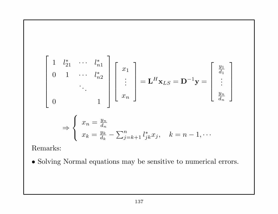
1 l∗21 · · · l∗n1
0 1 · · · l∗n2
. . .
0 1
x1
...
xn
= LHxLS = D−1y =
y1
d1
...
yn
dn
⇒
xn = yn
dn
xk = yk
dk−∑n
j=k+1 l∗jkxj , k = n− 1, · · ·
Remarks:
• Solving Normal equations may be sensitive to numerical errors.
137

Ex.
3 3− δ4 4 + δ
x1
x2
=
−1
1
, Ax = b
where δ is a small number.
Exact solution:
x1
x2
=
− 1
δ
1δ
Assume that due to truncation errors, δ2 = 0.
AHA.=
25 25 + δ
25 + δ 25 + 2δ
,AHb =
1
1 + 2δ
.
138
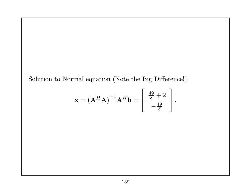
Solution to Normal equation (Note the Big Difference!):
x =(AHA
)−1AHb =
49δ
+ 2
− 49δ
.
139
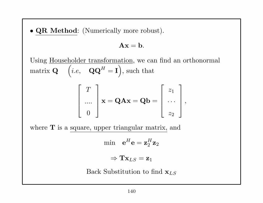
• QR Method: (Numerically more robust).
Ax = b.
Using Householder transformation, we can find an orthonormal
matrix Q(
i.e, QQH = I)
, such that
T
....
0
x = QAx = Qb =
z1
· · ·z2
,
where T is a square, upper triangular matrix, and
min eHe = zH2 z2
⇒ TxLS = z1
Back Substitution to find xLS
140
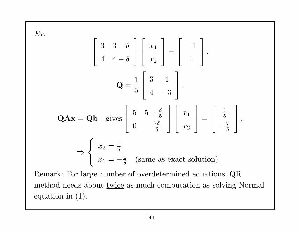
Ex.
3 3− δ4 4− δ
x1
x2
=
−1
1
.
Q =1
5
3 4
4 −3
.
QAx = Qb gives
5 5 + δ
5
0 − 7δ5
x1
x2
=
15
− 75
.
⇒
x2 = 1δ
x1 = − 1δ
(same as exact solution)
Remark: For large number of overdetermined equations, QR
method needs about twice as much computation as solving Normal
equation in (1).
141
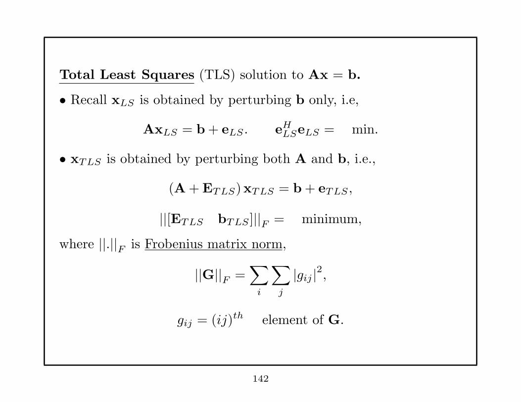
Total Least Squares (TLS) solution to Ax = b.
• Recall xLS is obtained by perturbing b only, i.e,
AxLS = b + eLS . eHLSeLS = min.
• xTLS is obtained by perturbing both A and b, i.e.,
(A + ETLS)xTLS = b + eTLS ,
||[ETLS bTLS ]||F = minimum,
where ||.||F is Frobenius matrix norm,
||G||F =∑
i
∑
j
|gij |2,
gij = (ij)th element of G.
142
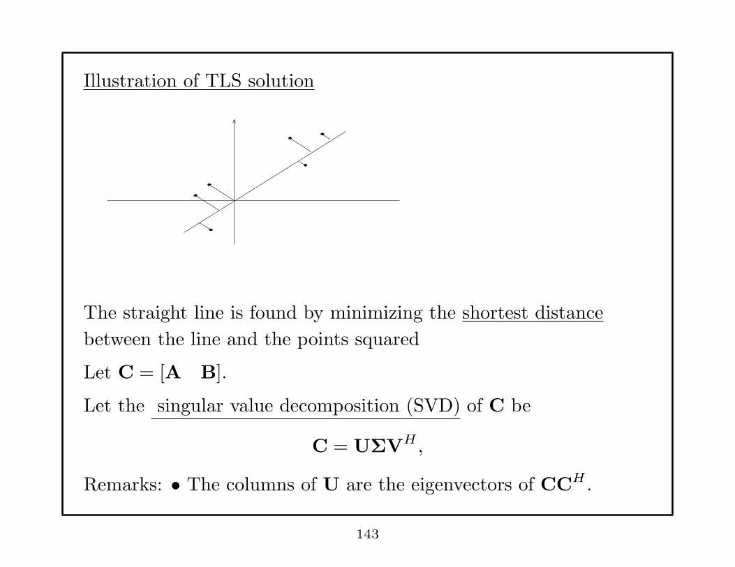
Illustration of TLS solution
The straight line is found by minimizing the shortest distance
between the line and the points squared
Let C = [A B].
Let the singular value decomposition (SVD) of C be
C = UΣVH ,
Remarks: • The columns of U are the eigenvectors of CCH .
143
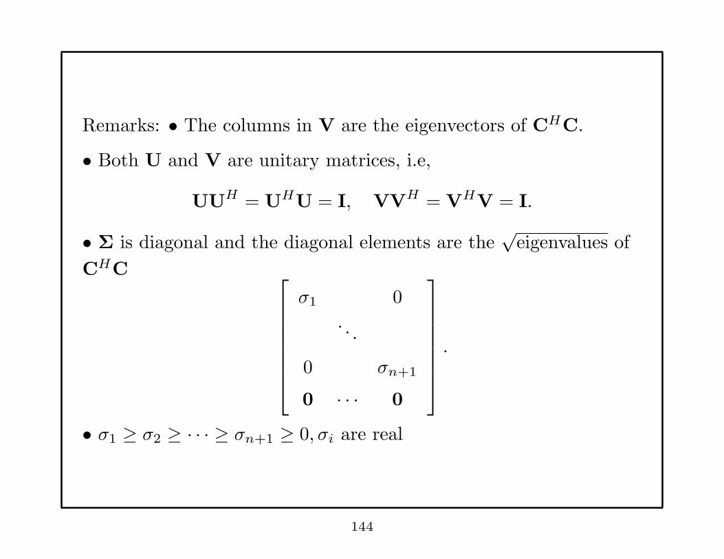
Remarks: • The columns in V are the eigenvectors of CHC.
• Both U and V are unitary matrices, i.e,
UUH = UHU = I, VVH = VHV = I.
• Σ is diagonal and the diagonal elements are the√
eigenvalues of
CHC
σ1 0
. . .
0 σn+1
0 · · · 0
.
• σ1 ≥ σ2 ≥ · · · ≥ σn+1 ≥ 0, σi are real
144
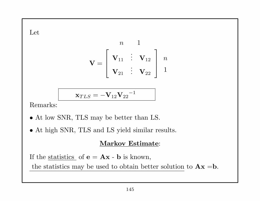
Let
n 1
V =
V11
... V12
V21
... V22
n
1
xTLS = −V12V22−1
Remarks:
• At low SNR, TLS may be better than LS.
• At high SNR, TLS and LS yield similar results.
Markov Estimate:
If the statistics of e = Ax - b is known,
the statistics may be used to obtain better solution to Ax =b.
145
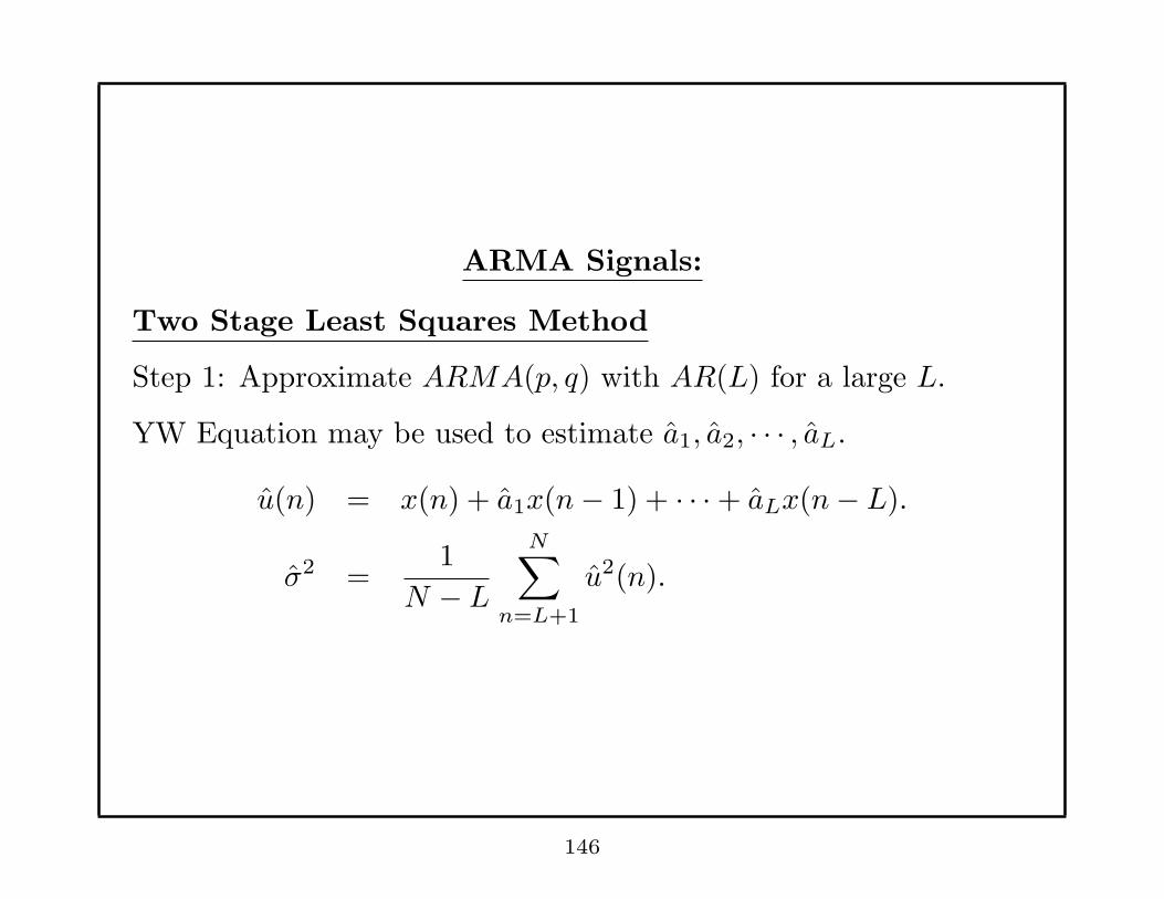
ARMA Signals:
Two Stage Least Squares Method
Step 1: Approximate ARMA(p, q) with AR(L) for a large L.
YW Equation may be used to estimate a1, a2, · · · , aL.
u(n) = x(n) + a1x(n− 1) + · · ·+ aLx(n− L).
σ2 =1
N − L
N∑
n=L+1
u2(n).
146
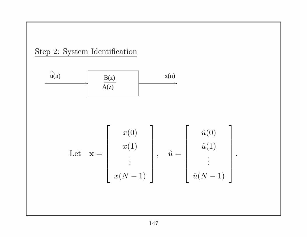
Step 2: System Identification
u(n) B(z)A(z)
x(n)
Let x =
x(0)
x(1)...
x(N − 1)
, u =
u(0)
u(1)...
u(N − 1)
.
147
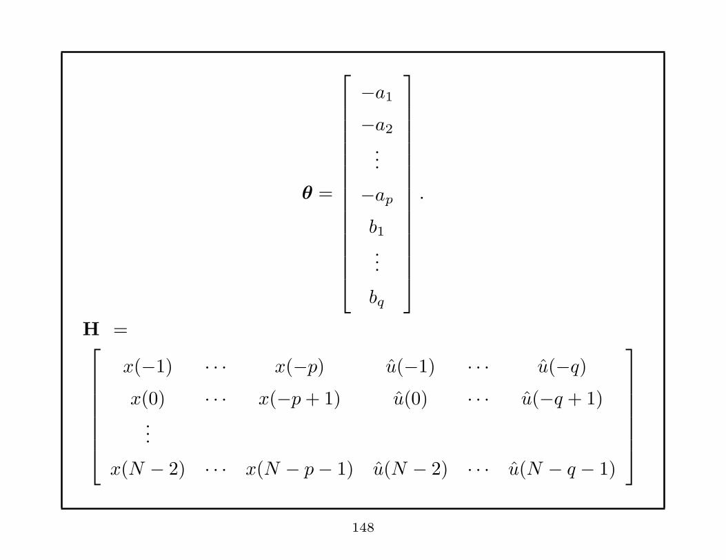
θ =
−a1
−a2
...
−ap
b1...
bq
.
H =
x(−1) · · · x(−p) u(−1) · · · u(−q)x(0) · · · x(−p+ 1) u(0) · · · u(−q + 1)
...
x(N − 2) · · · x(N − p− 1) u(N − 2) · · · u(N − q − 1)
148

x = Hθ + u (real signals) .
LS Solution ⇒ θ =(HT H
)−1HT (x− u)
Remarks:
• Any elements in H that are unknown are set to zero.
• QR Method may be used to solve the LS problem.
Step 3:
P (ω) = σ2
∣∣∣∣∣
1 + b1e−jω + · · ·+ bqe
−jωq
1 + a1e−jω + · · ·+ ape−jωp
∣∣∣∣∣
2
Remark: The difficult case for this method is when ARMA zeroes
are near unit circle.
149

Further Topics on AR Signals:
Linear prediction of AR Processes
• Forward Linear Prediction
n-4 n
x(n)
n-3n-2
n-1
Samples used to predict x(n)
x(n) -m
+
e (n)
i=1 x(n-i)a
(n)x
-f
ff
i
150
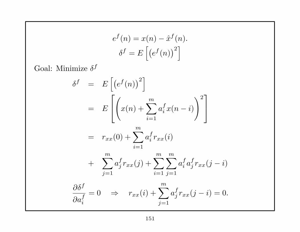
ef (n) = x(n)− xf (n).
δf = E[(ef (n)
)2]
Goal: Minimize δf
δf = E[(ef (n)
)2]
= E
(
x(n) +
m∑
i=1
afi x(n− i)
)2
= rxx(0) +
m∑
i=1
afi rxx(i)
+
m∑
j=1
afj rxx(j) +
m∑
i=1
m∑
j=1
afi a
fj rxx(j − i)
∂δf
∂afi
= 0 ⇒ rxx(i) +m∑
j=1
afj rxx(j − i) = 0.
151
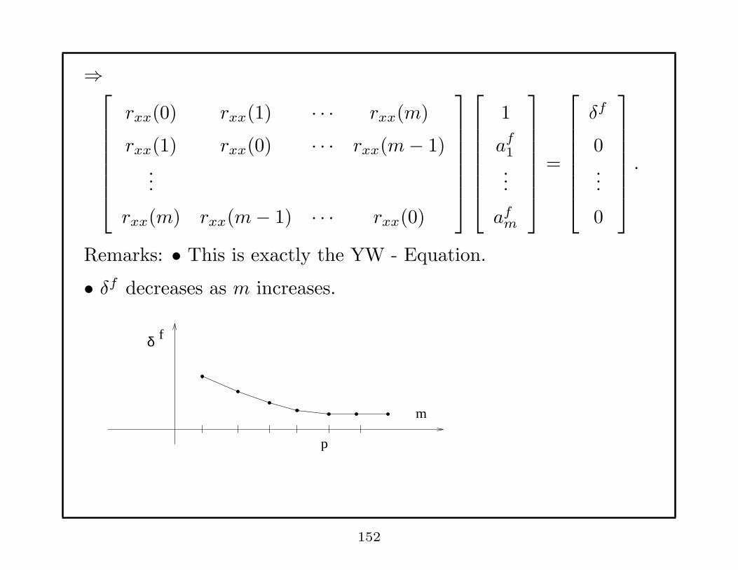
⇒
rxx(0) rxx(1) · · · rxx(m)
rxx(1) rxx(0) · · · rxx(m− 1)...
rxx(m) rxx(m− 1) · · · rxx(0)
1
af1
...
afm
=
δf
0...
0
.
Remarks: • This is exactly the YW - Equation.
• δf decreases as m increases.
p
m
fδ
152
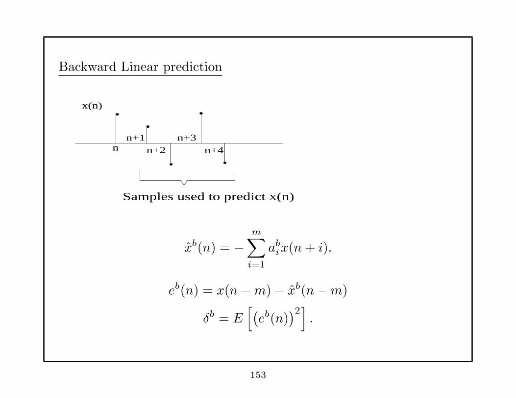
Backward Linear prediction
Samples used to predict x(n)
n+2n+3
n+4 n
x(n)
n+1
xb(n) = −m∑
i=1
abix(n+ i).
eb(n) = x(n−m)− xb(n−m)
δb = E[(eb(n)
)2]
.
153
To minimize δb, we obtain
rxx(0) rxx(1) · · · rxx(m)...
rxx(m) rxx(m− 1) · · · rxx(0)
1
ab1
...
abm
=
δb
0...
0
.
⇒ afi = ab
i , for all i
δf = δb.
154

Consider an AR(p) model and the notation in LDA:
Let m = 1, 2, · · · , p
efm(n) = x(n) +
m∑
i=1
afm,ix(n− i)
=[
x(n) x(n− 1) · · · x(n−m)]
1
θm
.
ebm(n) = x(n−m) +
m∑
i=1
abm,ix(n−m+ i)
= [x(n−m) x(n−m+ 1) · · · x(n)]
1
θm
= [x(n) · · · x(n−m+ 1) x(n−m)]
θm
1
155

Recall LDA:
θm =
θm−1
0
+ km
θm−1
1
.
efm(n) =
[x(n) x(n− 1) · · · x(n−m)]
1
θm−1
0
+ km
0
θm−1
1
= [x(n) x(n− 1) · · · x(n−m+ 1)]
1
θm−1
+km [x(n− 1) x(n− 2) · · · x(n−m)]
θm−1
1
156
efm(n) = e
fm−1(n) + kme
bm−1(n− 1).
Similarly,
ebm(n) = eb
m−1(n− 1) + kmefm−1(n).
157
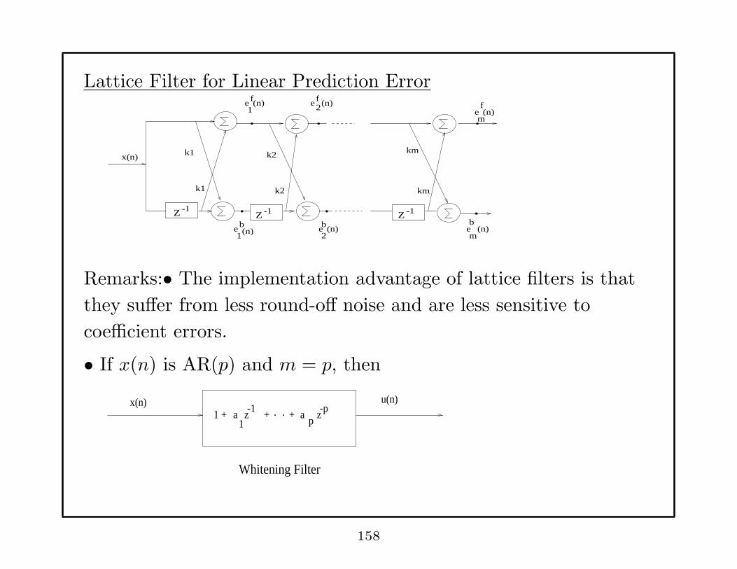
Lattice Filter for Linear Prediction Error
Z -1 Z -1 Z -1
k1 k2 km
k1 k2 km
x(n)
ef1
(n) e2 f (n)
eb 1(n) eb
2 (n)
ef
m(n)
(n)b
em
Remarks:• The implementation advantage of lattice filters is that
they suffer from less round-off noise and are less sensitive to
coefficient errors.
• If x(n) is AR(p) and m = p, then
x(n) u(n)1 +
Whitening Filter
a1
z -1 a p z + -p+
158
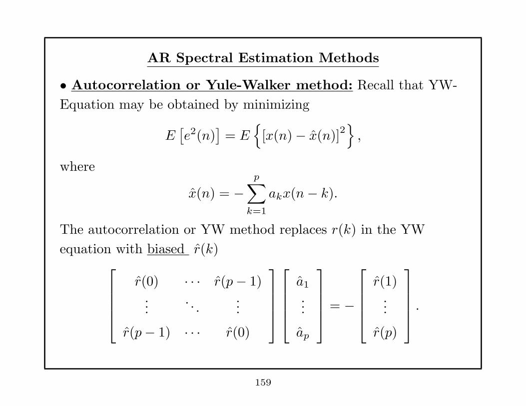
AR Spectral Estimation Methods
• Autocorrelation or Yule-Walker method: Recall that YW-
Equation may be obtained by minimizing
E[e2(n)
]= E
{
[x(n)− x(n)]2}
,
where
x(n) = −p∑
k=1
akx(n− k).
The autocorrelation or YW method replaces r(k) in the YW
equation with biased r(k)
r(0) · · · r(p− 1)...
. . ....
r(p− 1) · · · r(0)
a1
...
ap
= −
r(1)...
r(p)
.
159
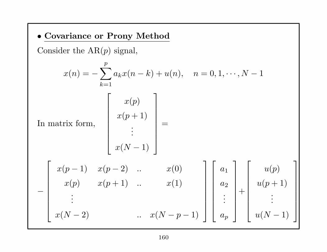
• Covariance or Prony Method
Consider the AR(p) signal,
x(n) = −p∑
k=1
akx(n− k) + u(n), n = 0, 1, · · · , N − 1
In matrix form,
x(p)
x(p+ 1)...
x(N − 1)
=
−
x(p− 1) x(p− 2) .. x(0)
x(p) x(p+ 1) .. x(1)...
x(N − 2) .. x(N − p− 1)
a1
a2
...
ap
+
u(p)
u(p+ 1)...
u(N − 1)
160

The Prony Method is to find LS solution to the overdetermined
equation
−
x(p− 1) · · · x(0)...
x(N − 2) · · · x(N − p− 1)
a1
...
ap
≈
x(p)...
x(N − 1)
.
Remarks:
• The Covariance or Prony Method minimizes
σ2 =1
N − p
N−1∑
n=p
u2(n) =1
N − p
N−1∑
n=p
[
x(n) +
p∑
k=1
akx(n− k)]2
161

• The Autocorrelation Method or YW-Method minimizes
σ2 =1
N
∞∑
n=−∞
[
x(n) +
p∑
k=1
akx(n− k)]2
where those x(n) that are NOT available are set to zero.
• For large N , the YW and Prony methods yield similar results.
• For small N , YW method gives poor performance. The Prony
method can give good estimates a1, · · · , ap for small N . The Prony
method gives exact estimates for x(n) =sum of sinusoids.
• Since biased r(k) are used in YW method, the estimated poles
are inside unit circle. Prony method does not guarantee stability.
162
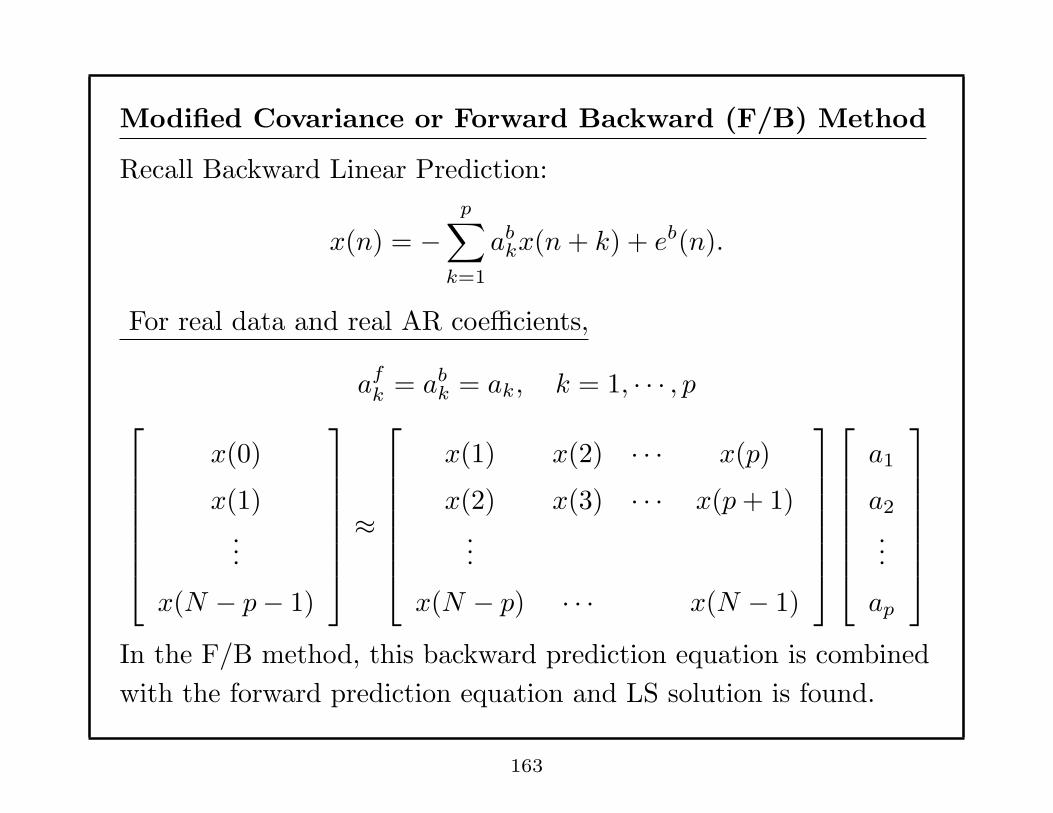
Modified Covariance or Forward Backward (F/B) Method
Recall Backward Linear Prediction:
x(n) = −p∑
k=1
abkx(n+ k) + eb(n).
For real data and real AR coefficients,
afk = ab
k = ak, k = 1, · · · , p
x(0)
x(1)...
x(N − p− 1)
≈
x(1) x(2) · · · x(p)
x(2) x(3) · · · x(p+ 1)...
x(N − p) · · · x(N − 1)
a1
a2
...
ap
In the F/B method, this backward prediction equation is combined
with the forward prediction equation and LS solution is found.
163
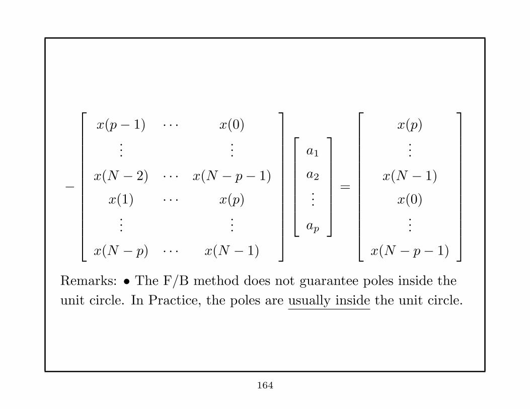
−
x(p− 1) · · · x(0)...
...
x(N − 2) · · · x(N − p− 1)
x(1) · · · x(p)...
...
x(N − p) · · · x(N − 1)
a1
a2
...
ap
=
x(p)...
x(N − 1)
x(0)...
x(N − p− 1)
Remarks: • The F/B method does not guarantee poles inside the
unit circle. In Practice, the poles are usually inside the unit circle.
164
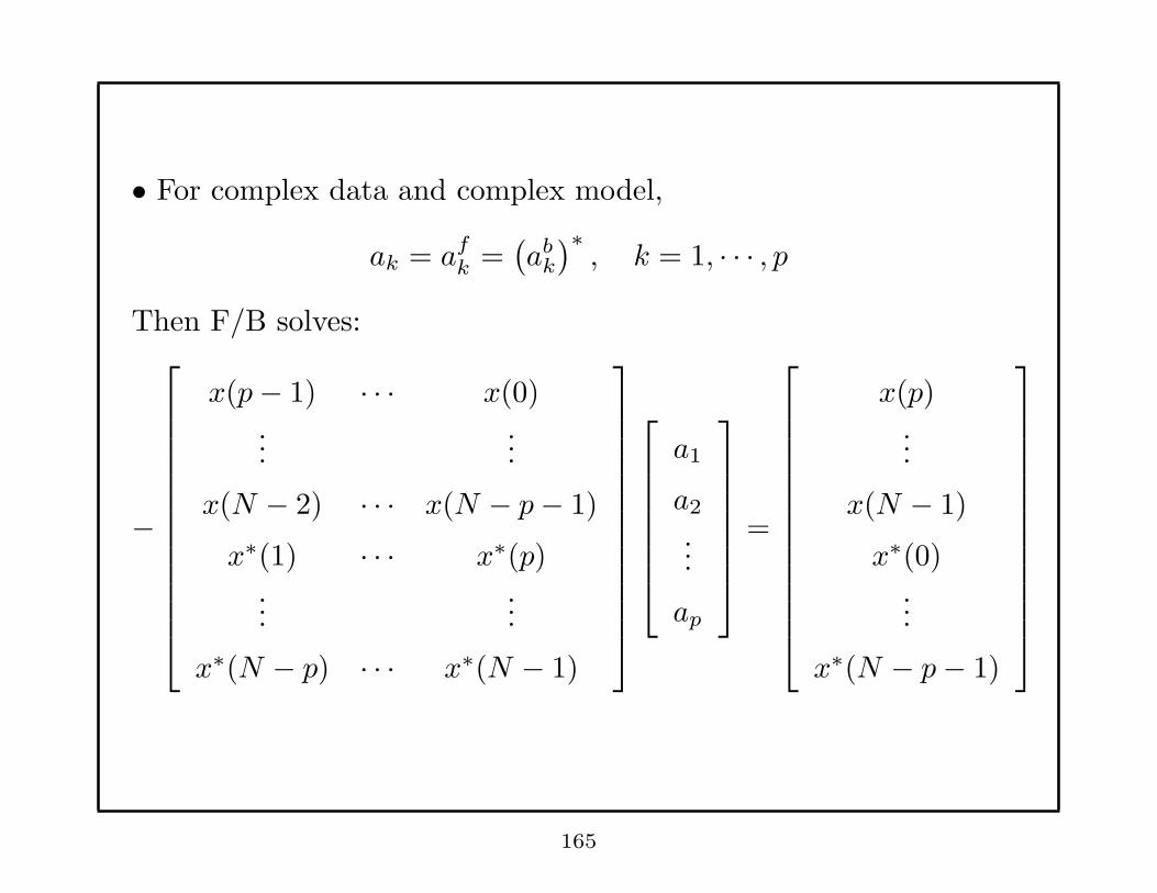
• For complex data and complex model,
ak = afk =
(ab
k
)∗, k = 1, · · · , p
Then F/B solves:
−
x(p− 1) · · · x(0)...
...
x(N − 2) · · · x(N − p− 1)
x∗(1) · · · x∗(p)...
...
x∗(N − p) · · · x∗(N − 1)
a1
a2
...
ap
=
x(p)...
x(N − 1)
x∗(0)...
x∗(N − p− 1)
165

Remarks on σ2:
• In YW method,
σ2 = r(0) +
p∑
k=1
akr(k).
• In Prony Method,
Let eLS =
e(p)...
e(N − 1)
σ2 =1
N − p
N−1∑
n=p
|e(n)|2
166
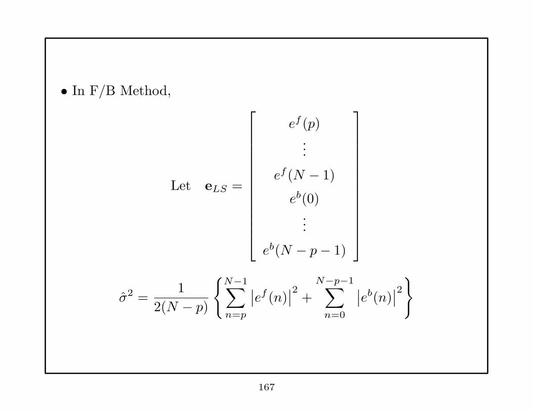
• In F/B Method,
Let eLS =
ef (p)...
ef (N − 1)
eb(0)...
eb(N − p− 1)
σ2 =1
2(N − p)
{N−1∑
n=p
∣∣ef (n)
∣∣2
+
N−p−1∑
n=0
∣∣eb(n)
∣∣2
}
167
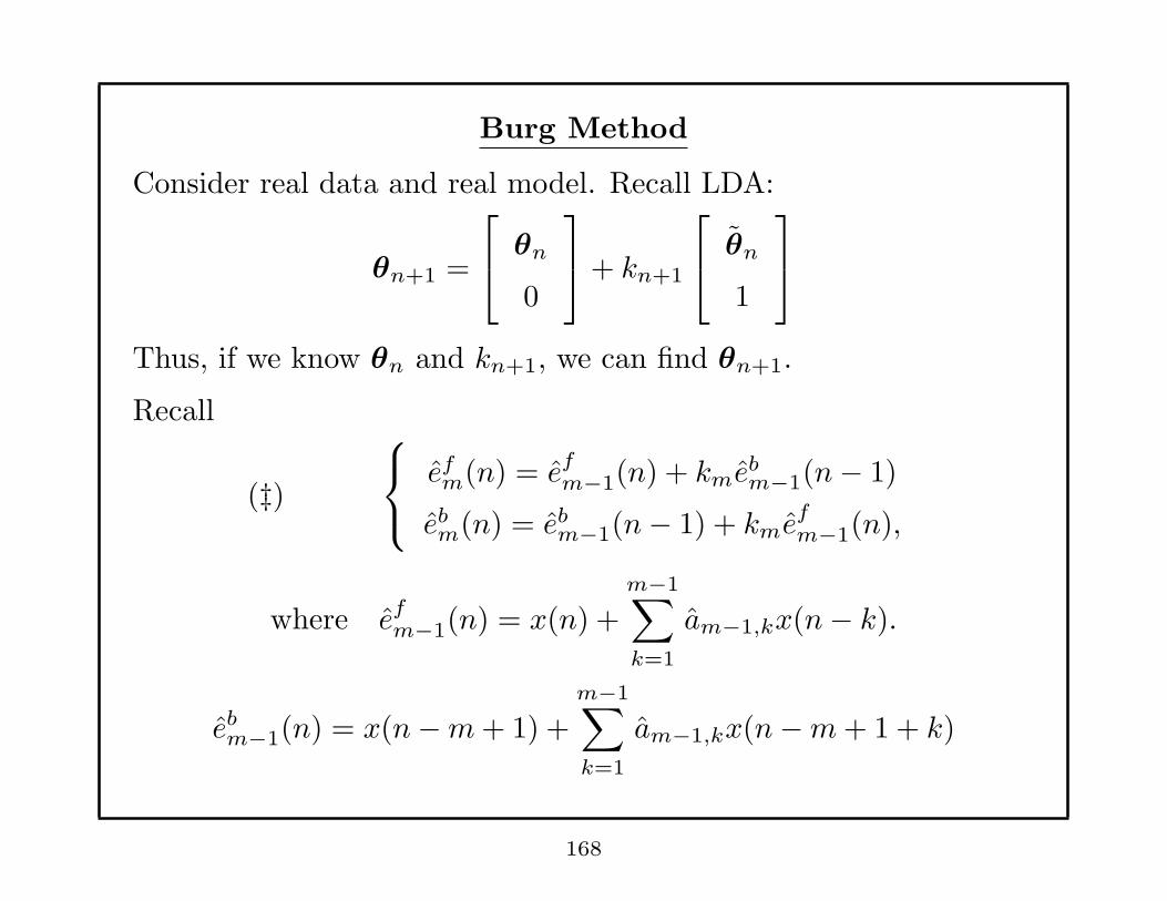
Burg Method
Consider real data and real model. Recall LDA:
θn+1 =
θn
0
+ kn+1
θn
1
Thus, if we know θn and kn+1, we can find θn+1.
Recall
(‡)
efm(n) = e
fm−1(n) + kme
bm−1(n− 1)
ebm(n) = eb
m−1(n− 1) + kmefm−1(n),
where efm−1(n) = x(n) +
m−1∑
k=1
am−1,kx(n− k).
ebm−1(n) = x(n−m+ 1) +
m−1∑
k=1
am−1,kx(n−m+ 1 + k)
168
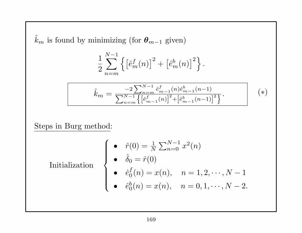
km is found by minimizing (for θm−1 given)
1
2
N−1∑
n=m
{[efm(n)
]2+[ebm(n)
]2}
.
km =−2∑
N−1
n=me
f
m−1(n)eb
m−1(n−1)∑
N−1
n=m
{[ef
m−1(n)]
2+[eb
m−1(n−1)]
2} . (∗)
Steps in Burg method:
Initialization
• r(0) = 1N
∑N−1n=0 x
2(n)
• δ0 = r(0)
• ef0 (n) = x(n), n = 1, 2, · · · , N − 1
• eb0(n) = x(n), n = 0, 1, · · · , N − 2.
169

For m = 1, 2, · · · , p,• Calculate km with (*)
• δm = δm−1(1− k2m)
• θm =
θm−1
0
+ km
˜θm−1
1
, ( θ1 = k1).
• Update efm(n) and eb
m(n) with (‡)Remarks: • δp = σ2.
• Since a2 + b2 ≥ 2ab,∣∣∣km
∣∣∣ < 1,
⇒ Burg Method gives poles that are inside unit circle.
• Different ways of calculating km are available.
170
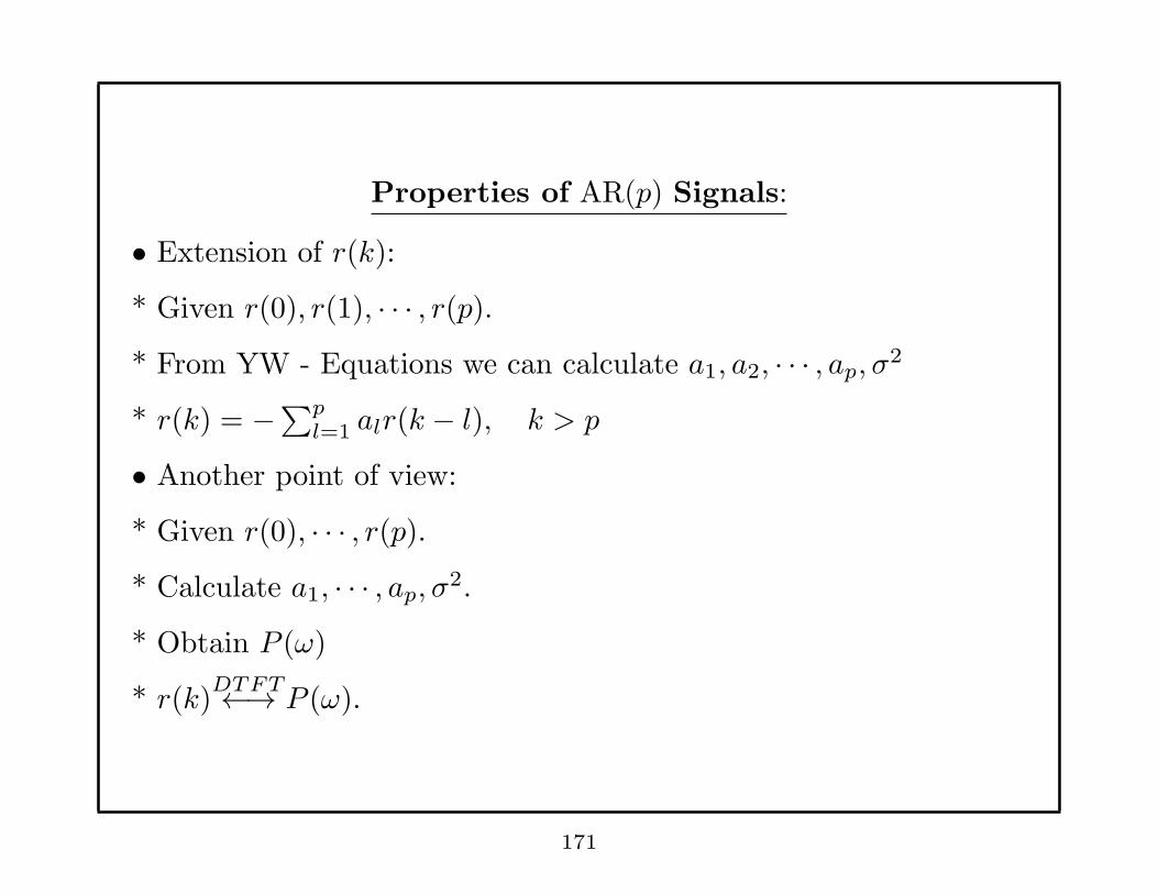
Properties of AR(p) Signals:
• Extension of r(k):
* Given r(0), r(1), · · · , r(p).* From YW - Equations we can calculate a1, a2, · · · , ap, σ
2
* r(k) = −∑p
l=1 alr(k − l), k > p
• Another point of view:
* Given r(0), · · · , r(p).* Calculate a1, · · · , ap, σ
2.
* Obtain P (ω)
* r(k)DTFT←→ P (ω).
171
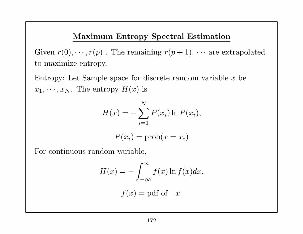
Maximum Entropy Spectral Estimation
Given r(0), · · · , r(p) . The remaining r(p+ 1), · · · are extrapolated
to maximize entropy.
Entropy: Let Sample space for discrete random variable x be
x1, · · · , xN . The entropy H(x) is
H(x) = −N∑
i=1
P (xi) lnP (xi),
P (xi) = prob(x = xi)
For continuous random variable,
H(x) = −∫ ∞
−∞f(x) ln f(x)dx.
f(x) = pdf of x.
172
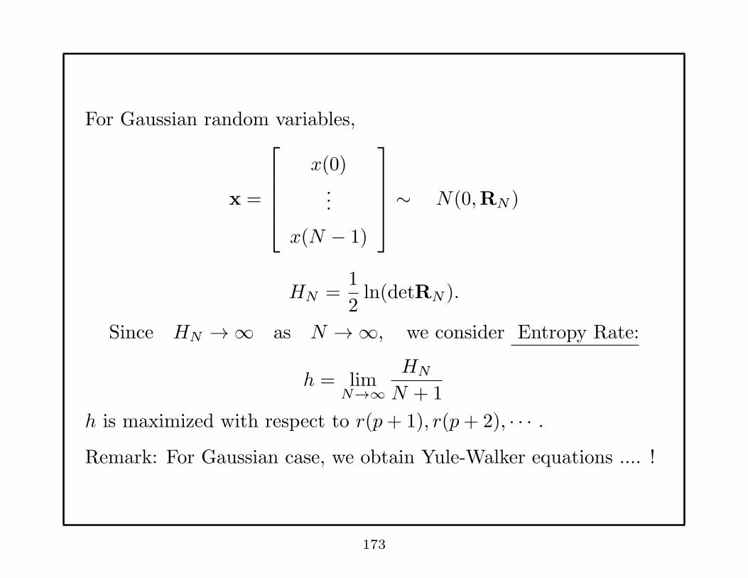
For Gaussian random variables,
x =
x(0)...
x(N − 1)
∼ N(0,RN )
HN =1
2ln(detRN ).
Since HN →∞ as N →∞, we consider Entropy Rate:
h = limN→∞
HN
N + 1
h is maximized with respect to r(p+ 1), r(p+ 2), · · · .Remark: For Gaussian case, we obtain Yule-Walker equations .... !
173

Maximum Likelihood Estimators:
• Exact ML Estimator:
u(n) 1
A(z)real inputs real outputs
x(n) , n = 0, ..., N-1
u(n) is Gaussian white noise with zero-mean.
⇒
E[u(n)] = 0,
V ar[u(n)] = σ2
E[u(i)u(j)] = 0, i 6= j,
The likelihood function is
f = f[x(0), · · · , x(N − 1)|a1, · · · , ap, σ
2]
The ML estimates of a1, · · · , ap, σ2 are found by maximizing f .
174

f = f[x(p), · · · , x(N − 1)|x(0), · · · , x(p− 1), a1, · · · , ap, σ
2]
f[x(0), · · · , x(p− 1)|a1, · · · , ap, σ
2]
* Consider first f1 = f[x(0), · · · , x(p− 1)|a1, · · · , ap, σ
2]
f1 =1
(2π)p2 det
12 (Rp)
exp
[
−1
2
(xT
0 R−1p x0
)]
.
x0 =
x(0)...
x(p− 1)
, Rp =
r(0) · · · r(p− 1)...
. . ....
r(p− 1) · · · r(0)
.
Remark: r(0), · · · , r(p− 1) are functions of a1, · · · , ap, σ2. (see, e.g.,
the YW system of equations)
175
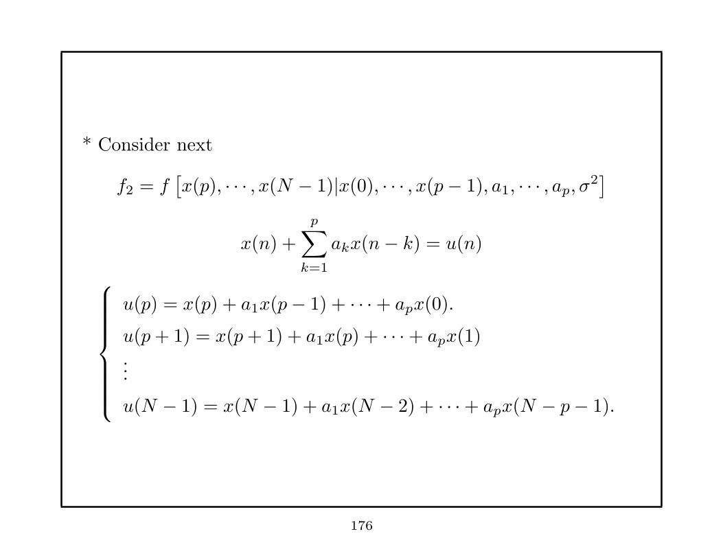
* Consider next
f2 = f[x(p), · · · , x(N − 1)|x(0), · · · , x(p− 1), a1, · · · , ap, σ
2]
x(n) +
p∑
k=1
akx(n− k) = u(n)
u(p) = x(p) + a1x(p− 1) + · · ·+ apx(0).
u(p+ 1) = x(p+ 1) + a1x(p) + · · ·+ apx(1)...
u(N − 1) = x(N − 1) + a1x(N − 2) + · · ·+ apx(N − p− 1).
176
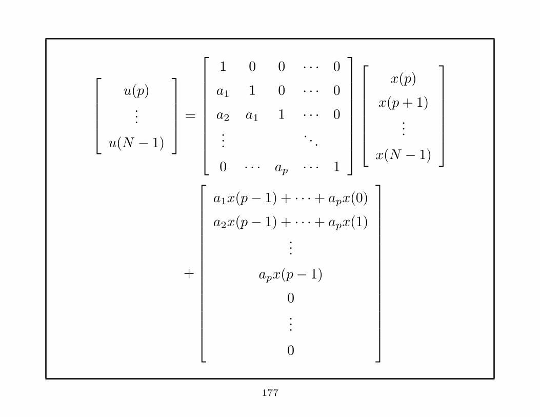
u(p)...
u(N − 1)
=
1 0 0 · · · 0
a1 1 0 · · · 0
a2 a1 1 · · · 0...
. . .
0 · · · ap · · · 1
x(p)
x(p+ 1)...
x(N − 1)
+
a1x(p− 1) + · · ·+ apx(0)
a2x(p− 1) + · · ·+ apx(1)...
apx(p− 1)
0...
0
177
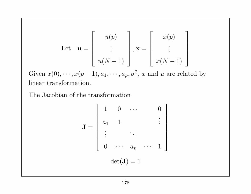
Let u =
u(p)...
u(N − 1)
,x =
x(p)...
x(N − 1)
Given x(0), · · · , x(p− 1), a1, · · · , ap, σ2, x and u are related by
linear transformation.
The Jacobian of the transformation
J =
1 0 · · · 0
a1 1...
.... . .
0 · · · ap · · · 1
det(J) = 1
178
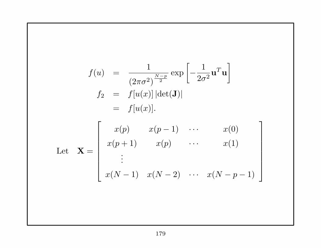
f(u) =1
(2πσ2)N−p
2
exp
[
− 1
2σ2uT u
]
f2 = f [u(x)] |det(J)|= f [u(x)].
Let X =
x(p) x(p− 1) · · · x(0)
x(p+ 1) x(p) · · · x(1)...
x(N − 1) x(N − 2) · · · x(N − p− 1)
179
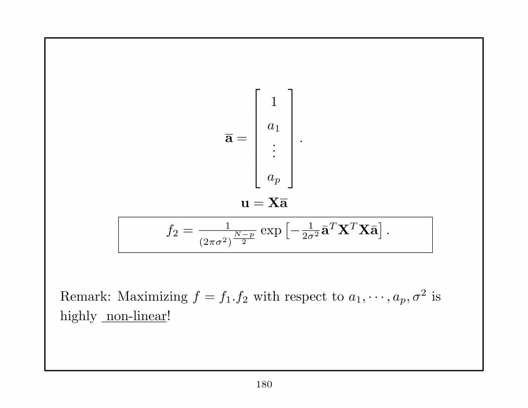
a =
1
a1
...
ap
.
u = Xa
f2 = 1
(2πσ2)N−p
2
exp[− 1
2σ2 aT XT Xa
].
Remark: Maximizing f = f1.f2 with respect to a1, · · · , ap, σ2 is
highly non-linear!
180
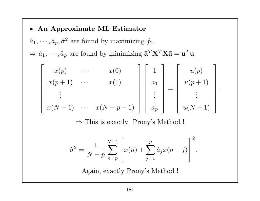
• An Approximate ML Estimator
a1, · · · , ap, σ2 are found by maximizing f2.
⇒ a1, · · · , ap are found by minimizing aT XT Xa = uT u
x(p) · · · x(0)
x(p+ 1) · · · x(1)...
x(N − 1) · · · x(N − p− 1)
1
a1
...
ap
=
u(p)
u(p+ 1)...
u(N − 1)
.
⇒ This is exactly Prony’s Method !
σ2 =1
N − p
N−1∑
n=p
x(n) +
p∑
j=1
ajx(n− j)
2
.
Again, exactly Prony’s Method !
181
Accuracy of AR PSD Estimators
• Accuracy Analysis is difficult.
• Results for large N are available due to Central Limit Theorem.
• For large N , the variances for a1, · · · , ap, k1, · · · , kp, σ2, P (ω)
are all proportional to 1N
. Biases ∝ 1N
.
182
AR Model Order Selection
Remarks:
• Order too low yields smoothed/biased PSD estimate.
• Order too high yields spurious peaks/large variance in PSD
estimate
• Almost all model order estimators are based on the estimate of
the power of linear prediction error, denoted δk, where k is the
model order chosen.
183
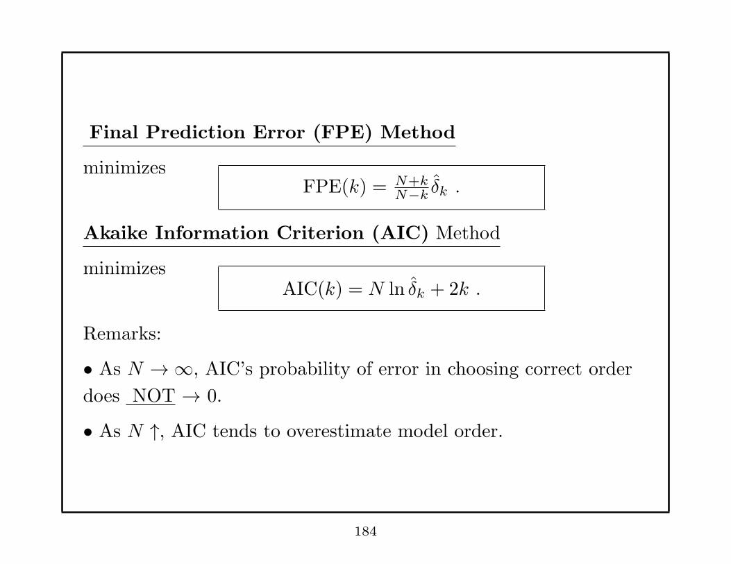
Final Prediction Error (FPE) Method
minimizesFPE(k) = N+k
N−kδk .
Akaike Information Criterion (AIC) Method
minimizesAIC(k) = N ln δk + 2k .
Remarks:
• As N →∞, AIC’s probability of error in choosing correct order
does NOT → 0.
• As N ↑, AIC tends to overestimate model order.
184
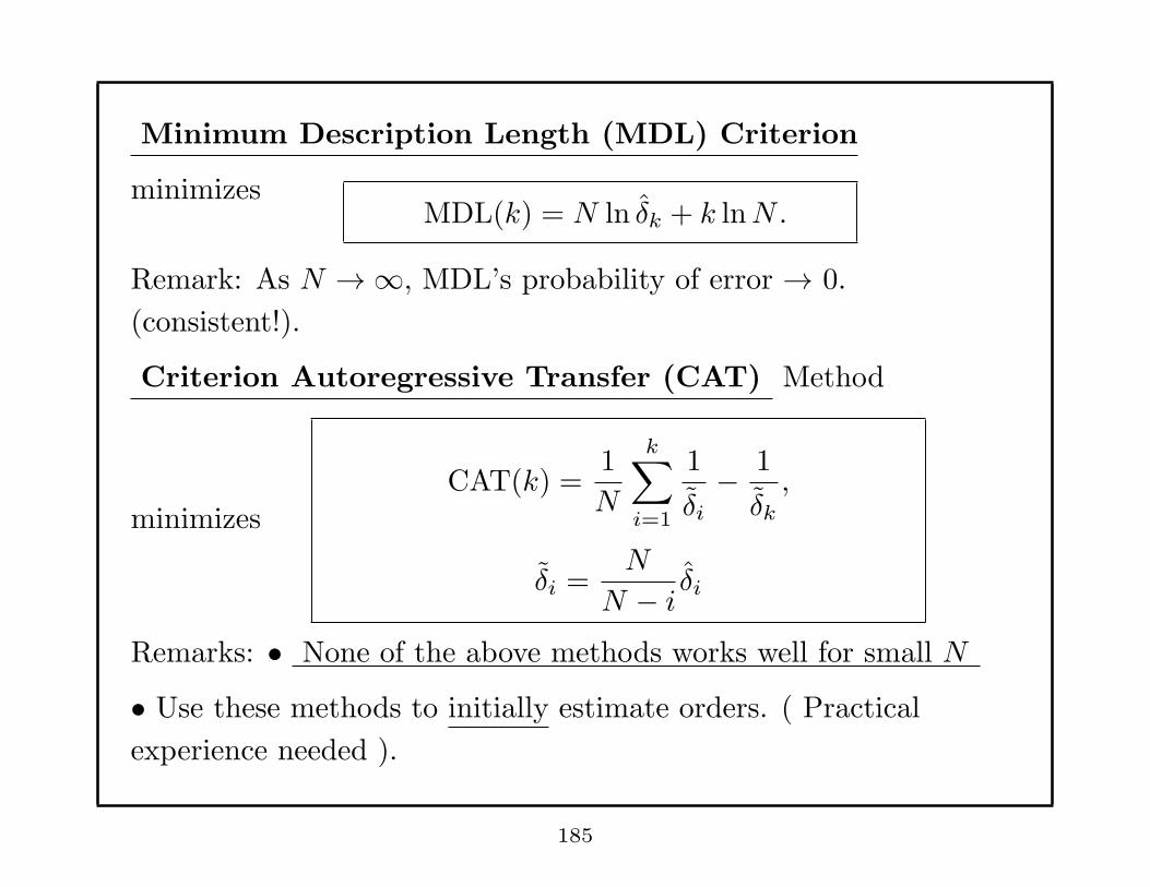
Minimum Description Length (MDL) Criterion
minimizesMDL(k) = N ln δk + k lnN .
Remark: As N →∞, MDL’s probability of error → 0.
(consistent!).
Criterion Autoregressive Transfer (CAT) Method
minimizes
CAT(k) =1
N
k∑
i=1
1
δi− 1
δk,
δi =N
N − i δi
Remarks: • None of the above methods works well for small N
• Use these methods to initially estimate orders. ( Practical
experience needed ).
185
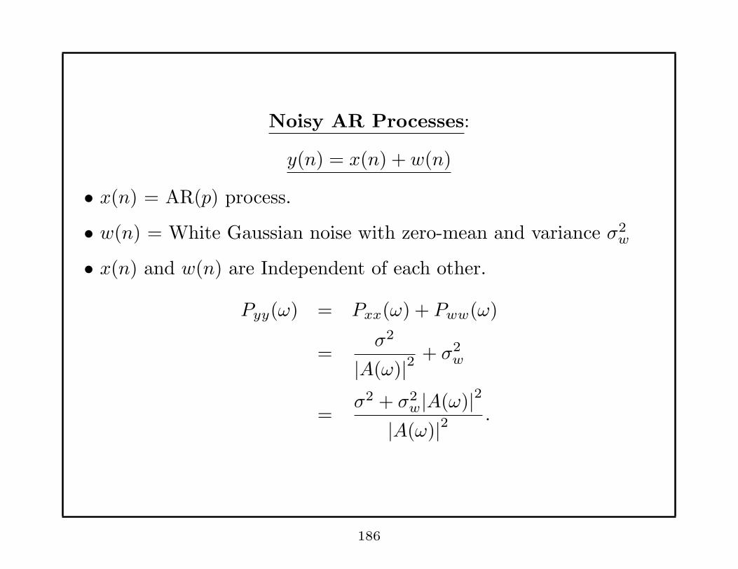
Noisy AR Processes:
y(n) = x(n) + w(n)
• x(n) = AR(p) process.
• w(n) = White Gaussian noise with zero-mean and variance σ2w
• x(n) and w(n) are Independent of each other.
Pyy(ω) = Pxx(ω) + Pww(ω)
=σ2
|A(ω)|2+ σ2
w
=σ2 + σ2
w|A(ω)|2
|A(ω)|2.
186
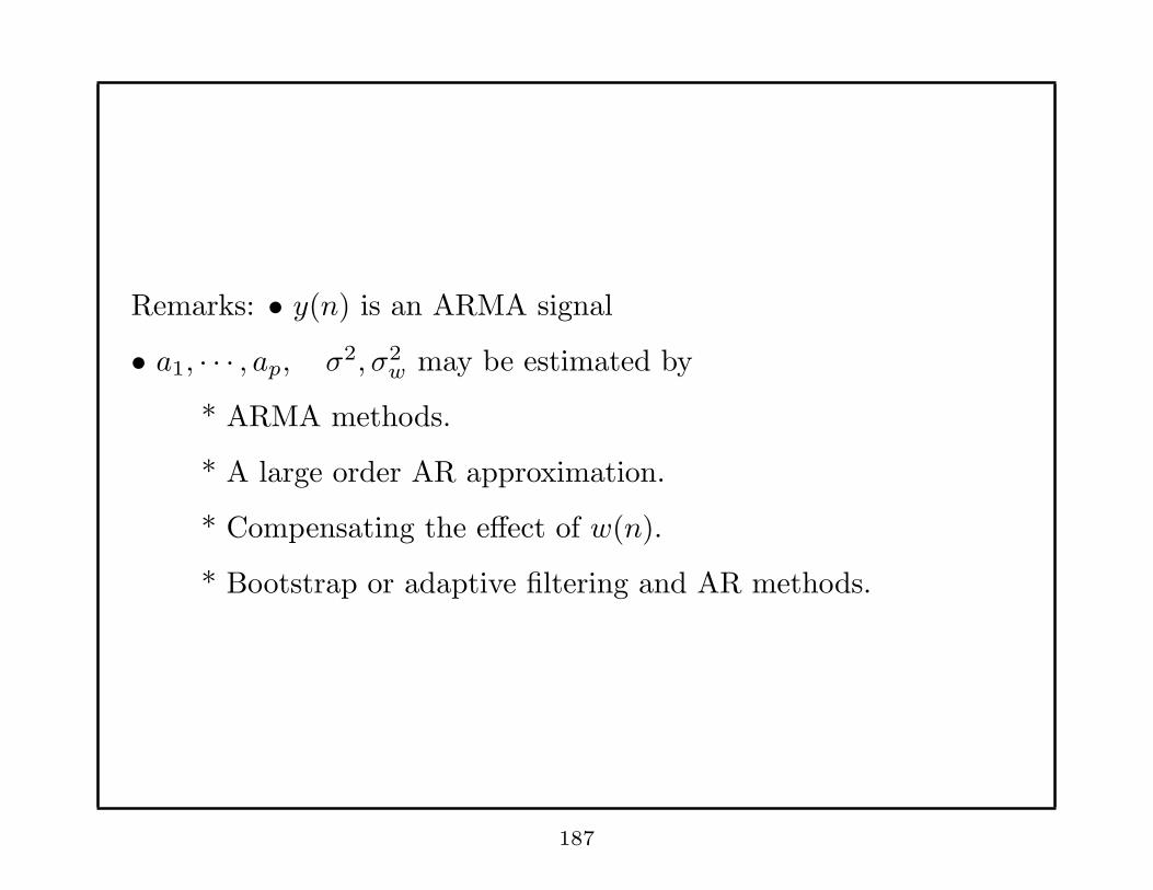
Remarks: • y(n) is an ARMA signal
• a1, · · · , ap, σ2, σ2w may be estimated by
* ARMA methods.
* A large order AR approximation.
* Compensating the effect of w(n).
* Bootstrap or adaptive filtering and AR methods.
187

Wiener Filter: (Wiener-Hopf Filter)
+y(n) = x(n) + w(n)
H(z) - e(n)
Desired Signalx(n)
x(n)
• H(z) is found by minimizing E[
|e(n)|2]
.
• H(z) depends on knowing Pxy(ω).
188

General Filtering Problem: (Complex Signals)
+y(n) = x(n) + w(n)
H(z) - e(n)
d(n) Desired Signal
Special case of d(n): d(n) = x(n+m):
1.) m > 0, m - step ahead prediction.
2.) m = 0, filtering problem
3.) m < 0, smoothing problem.
189
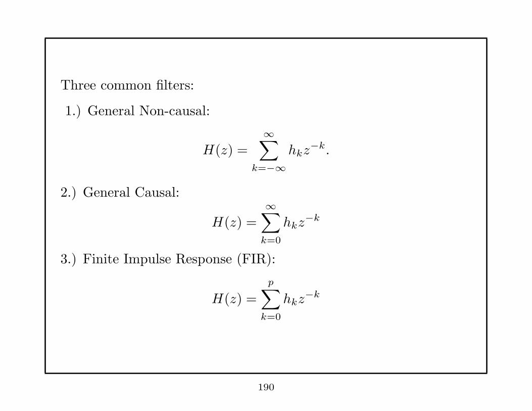
Three common filters:
1.) General Non-causal:
H(z) =∞∑
k=−∞hkz
−k.
2.) General Causal:
H(z) =
∞∑
k=0
hkz−k
3.) Finite Impulse Response (FIR):
H(z) =
p∑
k=0
hkz−k
190

Case 1: Non-causal Filter.
E = E{
|e(n)|2}
= E
{[
d(n)−∞∑
k=−∞hky(n− k)
][
d(n)−∞∑
l=−∞hly(n− l)
]∗}
= rdd(0)−∞∑
l=−∞h∗
l rdy(l)−∞∑
k=−∞hkr
∗dy(k)
+∞∑
k=−∞
∞∑
l=−∞ryy(l − k)hkh
∗l
Remark: For Causal and FIR filters, only limits of sums differ.
Let hi = αi + jβi
∂E
∂αi
= 0,∂E
∂βi
= 0.
⇒ rdy(i) =
∞∑
k=−∞ho
kryy(i− k), ∀i
191
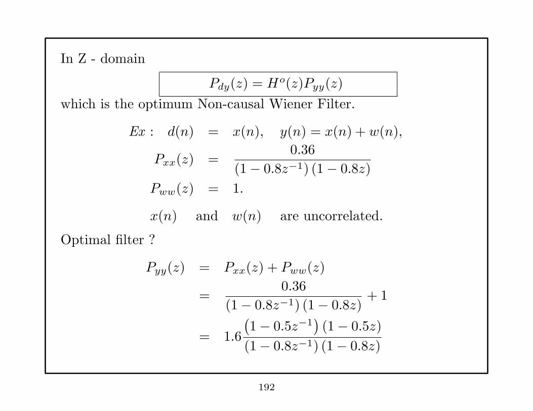
In Z - domain
Pdy(z) = Ho(z)Pyy(z)
which is the optimum Non-causal Wiener Filter.
Ex : d(n) = x(n), y(n) = x(n) + w(n),
Pxx(z) =0.36
(1− 0.8z−1) (1− 0.8z)
Pww(z) = 1.
x(n) and w(n) are uncorrelated.
Optimal filter ?
Pyy(z) = Pxx(z) + Pww(z)
=0.36
(1− 0.8z−1) (1− 0.8z)+ 1
= 1.6
(1− 0.5z−1
)(1− 0.5z)
(1− 0.8z−1) (1− 0.8z)
192
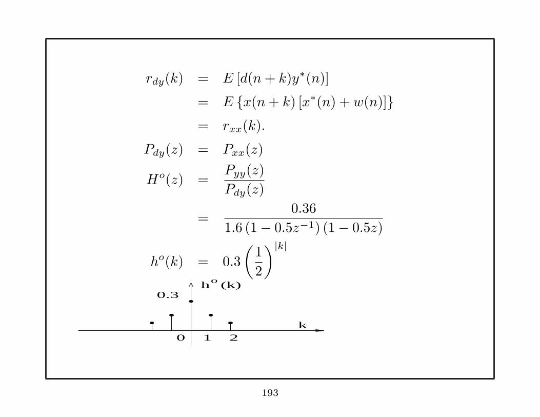
rdy(k) = E [d(n+ k)y∗(n)]
= E {x(n+ k) [x∗(n) + w(n)]}= rxx(k).
Pdy(z) = Pxx(z)
Ho(z) =Pyy(z)
Pdy(z)
=0.36
1.6 (1− 0.5z−1) (1− 0.5z)
ho(k) = 0.3
(1
2
)|k|
h
k0 1 2
o (k) 0.3
193
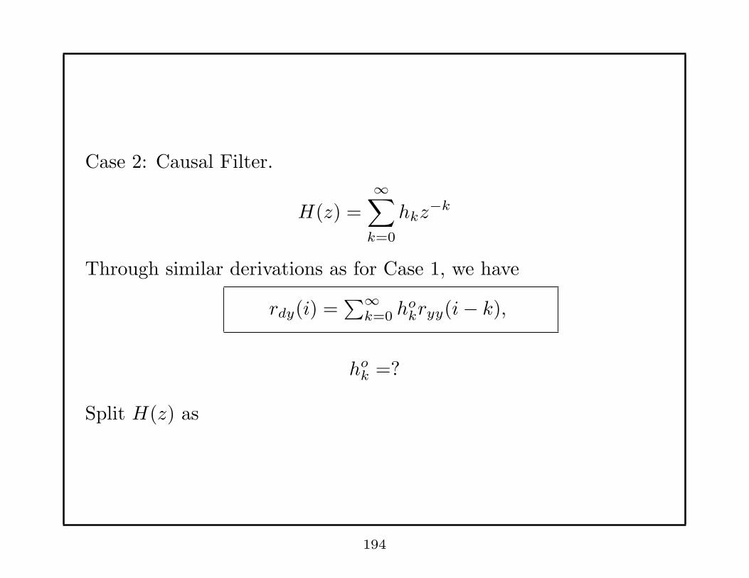
Case 2: Causal Filter.
H(z) =∞∑
k=0
hkz−k
Through similar derivations as for Case 1, we have
rdy(i) =∑∞
k=0 hokryy(i− k),
hok =?
Split H(z) as
194
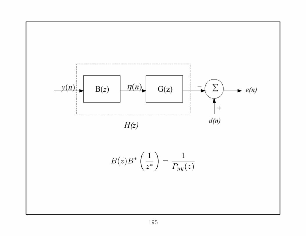
B(z)B∗(
1
z∗
)
=1
Pyy(z)
195
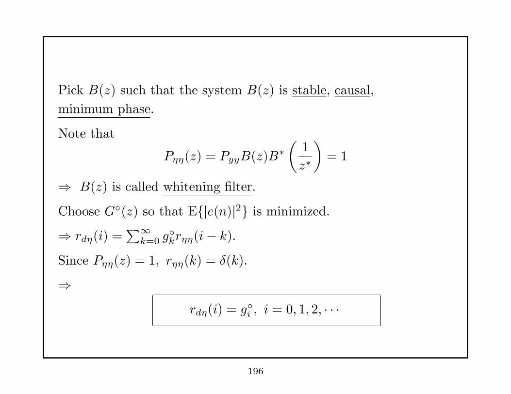
Pick B(z) such that the system B(z) is stable, causal,
minimum phase.
Note that
Pηη(z) = PyyB(z)B∗(
1
z∗
)
= 1
⇒ B(z) is called whitening filter.
Choose G◦(z) so that E{|e(n)|2} is minimized.
⇒ rdη(i) =∑∞
k=0 g◦krηη(i− k).
Since Pηη(z) = 1, rηη(k) = δ(k).
⇒rdη(i) = g◦
i , i = 0, 1, 2, · · ·
196
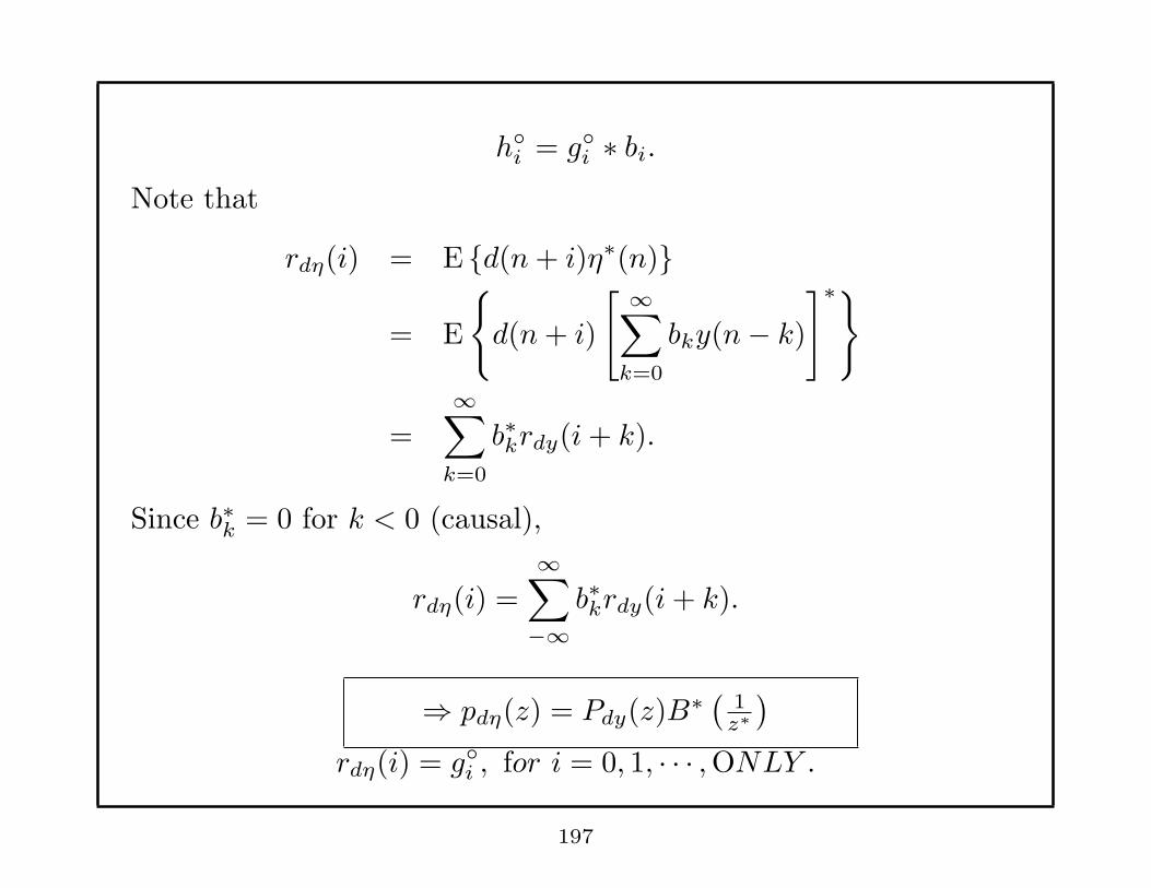
h◦i = g◦
i ∗ bi.Note that
rdη(i) = E {d(n+ i)η∗(n)}
= E
{
d(n+ i)
[ ∞∑
k=0
bky(n− k)]∗}
=
∞∑
k=0
b∗krdy(i+ k).
Since b∗k = 0 for k < 0 (causal),
rdη(i) =∞∑
−∞b∗krdy(i+ k).
⇒ pdη(z) = Pdy(z)B∗ ( 1z∗
)
rdη(i) = g◦i , for i = 0, 1, · · · ,ONLY .
197
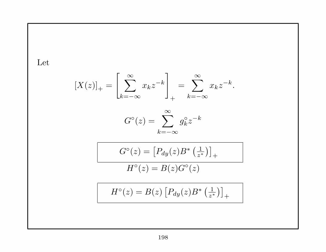
Let
[X(z)]+ =
[ ∞∑
k=−∞xkz
−k
]
+
=∞∑
k=−∞xkz
−k.
G◦(z) =
∞∑
k=−∞g◦
kz−k
G◦(z) =[Pdy(z)B∗ ( 1
z∗
)]
+
H◦(z) = B(z)G◦(z)
H◦(z) = B(z)[Pdy(z)B∗ ( 1
z∗
)]
+
198
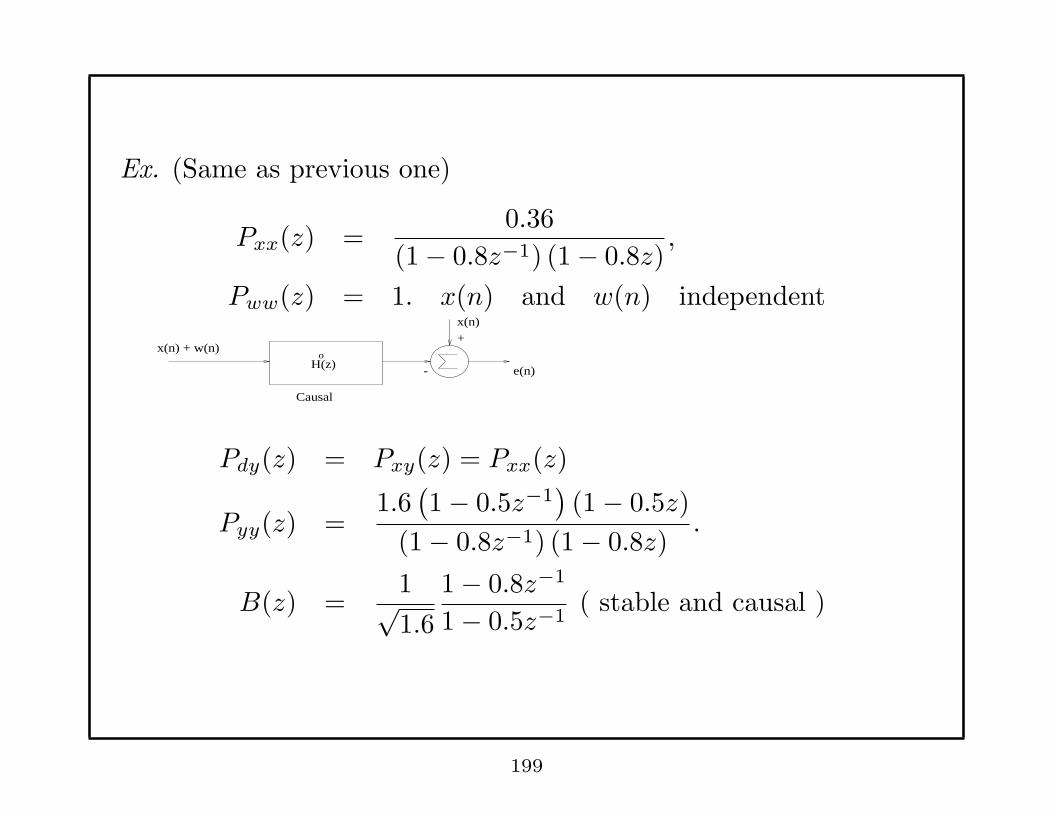
Ex. (Same as previous one)
Pxx(z) =0.36
(1− 0.8z−1) (1− 0.8z),
Pww(z) = 1. x(n) and w(n) independent
x(n)+
- e(n)
x(n) + w(n) H(z)
o
Causal
Pdy(z) = Pxy(z) = Pxx(z)
Pyy(z) =1.6(1− 0.5z−1
)(1− 0.5z)
(1− 0.8z−1) (1− 0.8z).
B(z) =1√1.6
1− 0.8z−1
1− 0.5z−1( stable and causal )
199
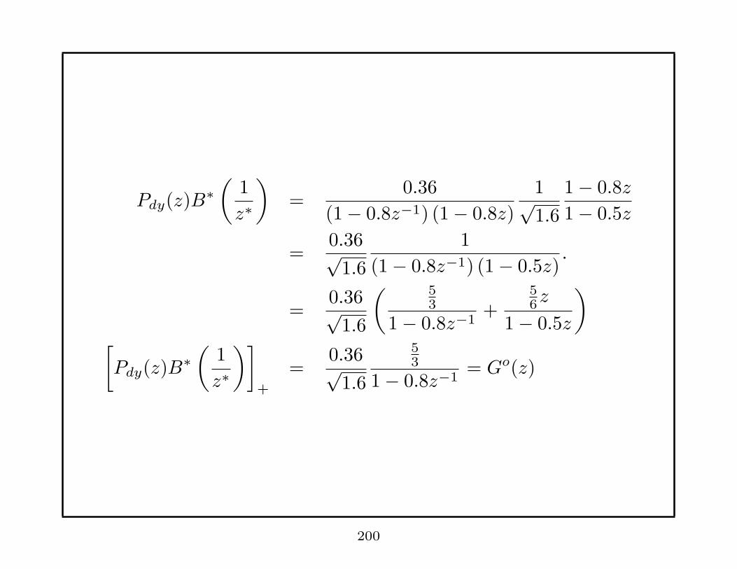
Pdy(z)B∗(
1
z∗
)
=0.36
(1− 0.8z−1) (1− 0.8z)
1√1.6
1− 0.8z
1− 0.5z
=0.36√
1.6
1
(1− 0.8z−1) (1− 0.5z).
=0.36√
1.6
( 53
1− 0.8z−1+
56z
1− 0.5z
)
[
Pdy(z)B∗(
1
z∗
)]
+
=0.36√
1.6
53
1− 0.8z−1= Go(z)
200
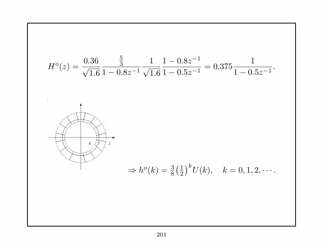
Ho(z) =0.36√
1.6
53
1− 0.8z−1
1√1.6
1− 0.8z−1
1− 0.5z−1= 0.375
1
1− 0.5z−1.
⇒ ho(k) = 38
(12
)kU(k), k = 0, 1, 2, · · · .
201

Case 3: FIR Filter:
H(z) =
p∑
k=0
hkz−k
Again, we can show similarly
rdy(i) =
p∑
k=0
hokryy(i− k).
rdy(0)
rdy(1)...
rdy(p)
=
ryy(0) ryy(−1) · · · ryy(−p)ryy(1) ryy(0) · · ·
.... . .
ryy(p) ryy(p− 1) · · · ryy(0)
ho0
ho1
...
hop
Remark: The Minimum error E is the smallest in case (1) and
largest in case (3).
202

Parametric Methods for Line Spectra
y(n) = x(n) + w(n)
x(n) =
K∑
k=1
αkej(ωkn+φk)
φk = Initial phases, independent of each other,
uniform distribution on [−π, π]
αk = amplitudes, constants, > 0
ωk = angular frequencies
w(n) = zero-mean white Gaussian Noise,
independent of φ1, · · · , φK
203
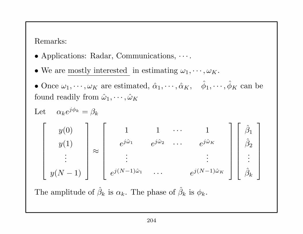
Remarks:
• Applications: Radar, Communications, · · · .• We are mostly interested in estimating ω1, · · · , ωK .
• Once ω1, · · · , ωK are estimated, α1, · · · , αK , φ1, · · · , φK can be
found readily from ω1, · · · , ωK
Let αkejφk = βk
y(0)
y(1)...
y(N − 1)
≈
1 1 · · · 1
ejω1 ejω2 · · · ejωK
......
ej(N−1)ω1 · · · ej(N−1)ωK
β1
β2
...
βk
The amplitude of βk is αk. The phase of βk is φk.
204
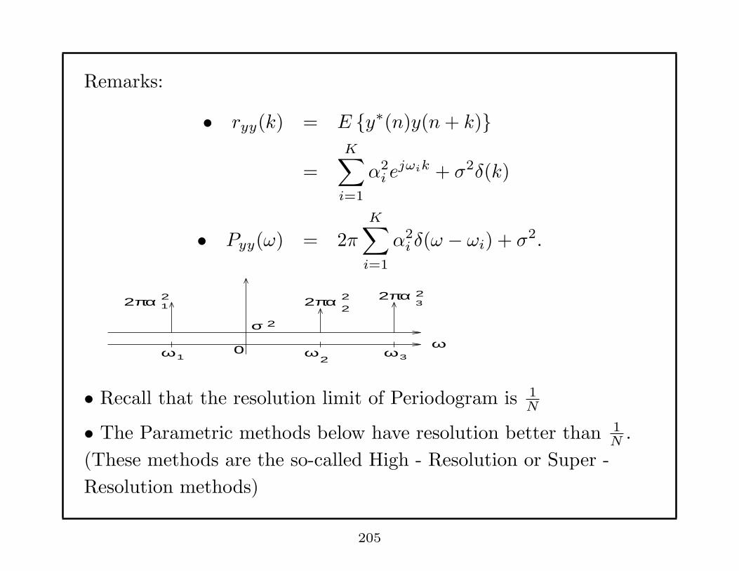
Remarks:
• ryy(k) = E {y∗(n)y(n+ k)}
=K∑
i=1
α2i e
jωik + σ2δ(k)
• Pyy(ω) = 2πK∑
i=1
α2i δ(ω − ωi) + σ2.
2π α 1
σ
2π α 2π α 3
2
2 2 2
ω ωω1 2 3
2
0 ω
• Recall that the resolution limit of Periodogram is 1N
• The Parametric methods below have resolution better than 1N
.
(These methods are the so-called High - Resolution or Super -
Resolution methods)
205
Maximum Likelihood Estimator
w(n) is assumed to be zero-mean circularly symmetric complex
Gaussian random variable with variance σ2.
The pdf of w(n) is N(0, σ2)
f (w(n)) =1
πσ2exp
{
−|w(n)|2σ2
}
.
Remark: • The real and imaginary parts of w(n) are real Gaussian
random variables with zero-mean and variance σ2
2 .
• The two parts are independent of each other.
206
f (w(0), · · · , w(N − 1)) =1
(πσ2)N
exp
{
−∑N−1
n=0 |w(n)|2
σ2
}
The likelihood function of y(0), · · · , y(N − 1) is
f = f (y(0), · · · , y(N − 1)) =1
(πσ2)N
exp
{
−∑N−1
n=0 |y(n)− x(n)|2
σ2
}
Remark: The ML estimates of
ω1, · · · , ωK , α1, · · · , αK , φ1, · · · , φK are found by maximizing f
with respect to ω1, · · · , ωK , α1, · · · , αK , φ1, · · · , φK .
Equivalently, we minimize
g =
N−1∑
n=0
∣∣∣∣∣y(n)−
K∑
k=1
αkej(ωkn+φk)
∣∣∣∣∣
2
207

Remarks: If w(n) is neither Gaussian nor white, minimizing g is
called the non-linear least-squares method, in general.
• Let y =
y(0)...
y(N − 1)
,β =
β1
...
βK
,ω =
ω1
...
ωK
B =
1 1 · · · 1
ejω1 ejω2 · · · ejωK
......
ej(N−1)ω1 · · · ej(N−1)ωK
208
g = (y −Bβ)H
(y −Bβ) .
=[
β −(BHB
)−1BHy
]H (BHB
) [
β −(BHB
)−1BHy
]
+ yHy − yHB(BHB
)−1BHy.
⇒ω = argmaxω
[
yHB(BHB
)−1BHy
]
.
β =(BHB
)−1BHy
∣∣∣ω=ω
.
Remarks: • ω is a consistent estimate of ω
209
• For large N ,
E[
(ω − ω) (ω − ω)H]
=6σ2
N3
1α2
1
. . .
1α2
K
= CRB
However,
• The maximization to obtain ω is difficult to implement.
* The search may not find global maximum.
* Computationally expensive.
210
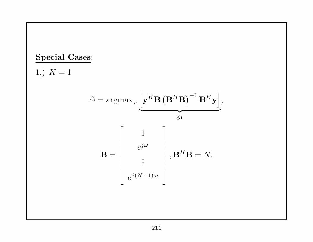
Special Cases:
1.) K = 1
ω = argmaxω
[
yHB(BHB
)−1BHy
]
︸ ︷︷ ︸
g1
,
B =
1
ejω
...
ej(N−1)ω
,BHB = N.
211
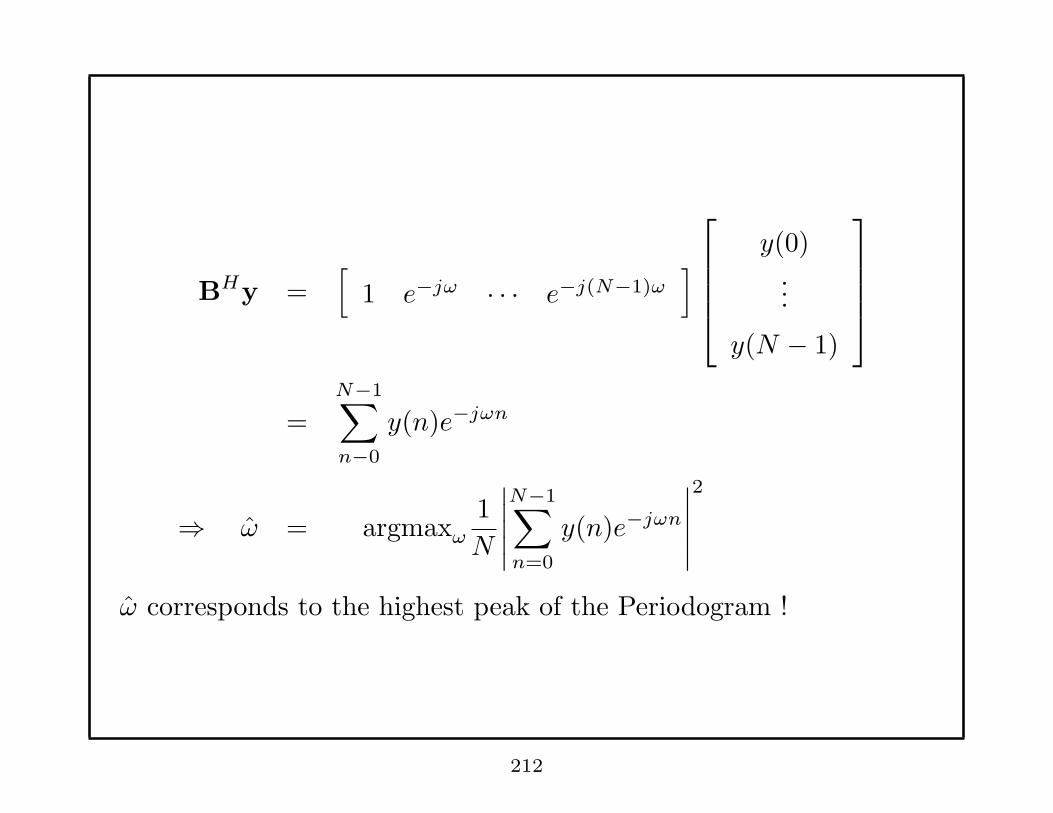
BHy =[
1 e−jω · · · e−j(N−1)ω]
y(0)...
y(N − 1)
=N−1∑
n−0
y(n)e−jωn
⇒ ω = argmaxω
1
N
∣∣∣∣∣
N−1∑
n=0
y(n)e−jωn
∣∣∣∣∣
2
ω corresponds to the highest peak of the Periodogram !
212
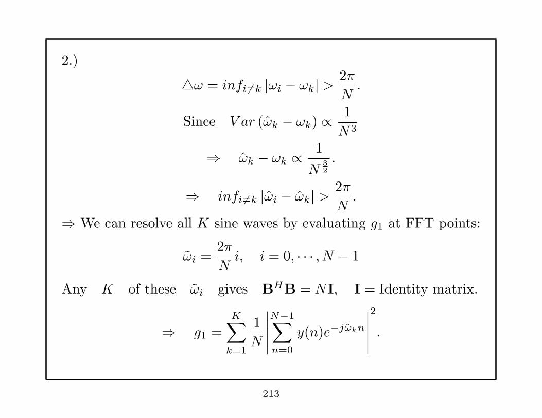
2.)
△ω = infi 6=k |ωi − ωk| >2π
N.
Since V ar (ωk − ωk) ∝ 1
N3
⇒ ωk − ωk ∝1
N32
.
⇒ infi 6=k |ωi − ωk| >2π
N.
⇒ We can resolve all K sine waves by evaluating g1 at FFT points:
ωi =2π
Ni, i = 0, · · · , N − 1
Any K of these ωi gives BHB = NI, I = Identity matrix.
⇒ g1 =
K∑
k=1
1
N
∣∣∣∣∣
N−1∑
n=0
y(n)e−jωkn
∣∣∣∣∣
2
.
213
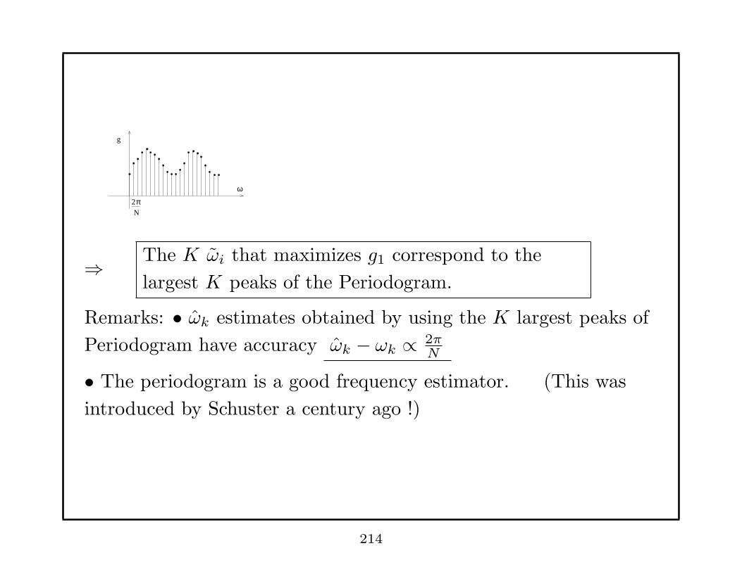
2πN
g
ω
⇒ The K ωi that maximizes g1 correspond to the
largest K peaks of the Periodogram.
Remarks: • ωk estimates obtained by using the K largest peaks of
Periodogram have accuracy ωk − ωk ∝ 2πN
• The periodogram is a good frequency estimator. (This was
introduced by Schuster a century ago !)
214

High - Resolution Methods
• Statistical Performance Close to ML estimator ( or CRB ) .
• Avoid Multidimensional search over parameter space.
• Do not depend on Resolution condition.
• All provide consistent estimates
• All give similar performance, especially for large N .
• Method of choice is a “ Matter - of - Taste ”.
215

Higher - Order Yule- Walker ( HOYW) Method:
Let xk(n) = αkej(ωkn+φk)
[1− ejωkz−1
]xk(n) = xk(n)− ejωkxk(n− 1)
= αkej(ωkn+φk) − ejωkαke
j[ωk(n−1)+φk]
= 0
⇒[1− ejωkz−1
]is an Annihilating filter for xk(n).
Let A(z) = ΠKk=1
(1− ejωkz−1
)
⇒A(z)x(n) = 0
y(n) = x(n) + w(n)
⇒ A(z)y(n) = A(z)w(n) (∗)
216
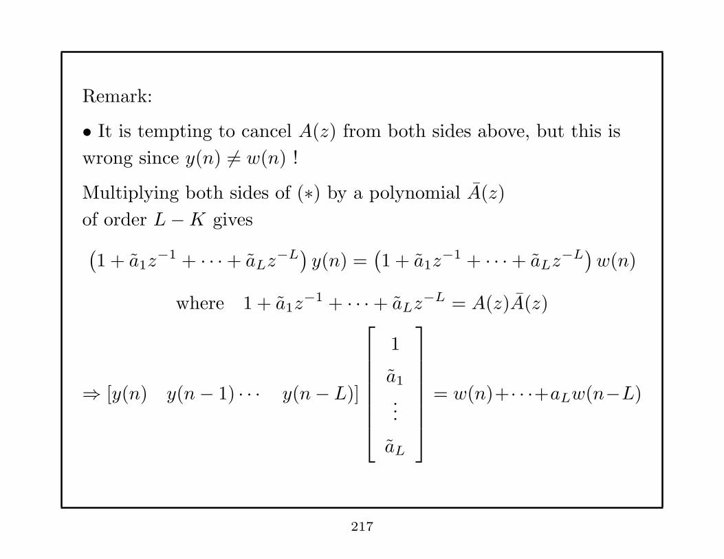
Remark:
• It is tempting to cancel A(z) from both sides above, but this is
wrong since y(n) 6= w(n) !
Multiplying both sides of (∗) by a polynomial A(z)
of order L−K gives
(1 + a1z
−1 + · · ·+ aLz−L)y(n) =
(1 + a1z
−1 + · · ·+ aLz−L)w(n)
where 1 + a1z−1 + · · ·+ aLz
−L = A(z)A(z)
⇒ [y(n) y(n− 1) · · · y(n− L)]
1
a1
...
aL
= w(n)+· · ·+aLw(n−L)
217

Multiplying both sides by
y∗(n− L− 1)...
y∗(n− L−M)
,
we get
ryy(L+ 1) · · · ryy(1)...
ryy(L+M) · · · ryy(M)
1
a1
...
aL
= 0.
⇒
ryy(L) · · · ryy(1)...
ryy(L+M − 1) · · · ryy(M)
a1
...
aL
= −
ryy(L+ 1)...
ryy(L+M)
⇒ Γa = −γ
218

Remarks:
• When y(0), · · · , y(N − 1) are the only data available, we first
estimate ryy(i) and replace ryy(i) in above equation with estimate
ryy(i)
• {ωK} are the angular positions of the K roots nearest the unit
circle
• Increasing L and M will
* give better performance due to using the information in
higher lags of r(i)
• Increasing L and M ‘too much’ will
* give worse performance due to increased variance in r(i) for
large i
219
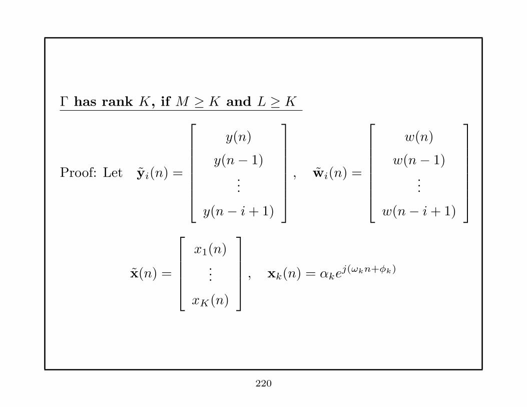
Γ has rank K, if M ≥ K and L ≥ K
Proof: Let yi(n) =
y(n)
y(n− 1)...
y(n− i+ 1)
, wi(n) =
w(n)
w(n− 1)...
w(n− i+ 1)
x(n) =
x1(n)...
xK(n)
, xk(n) = αke
j(ωkn+φk)
220
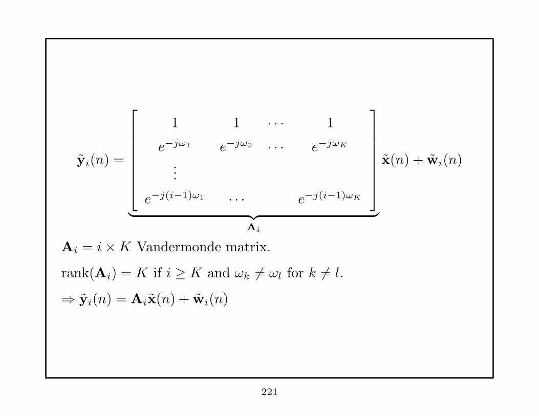
yi(n) =
1 1 · · · 1
e−jω1 e−jω2 · · · e−jωK
...
e−j(i−1)ω1 · · · e−j(i−1)ωK
︸ ︷︷ ︸
Ai
x(n) + wi(n)
Ai = i×K Vandermonde matrix.
rank(Ai) = K if i ≥ K and ωk 6= ωl for k 6= l.
⇒ yi(n) = Aix(n) + wi(n)
221
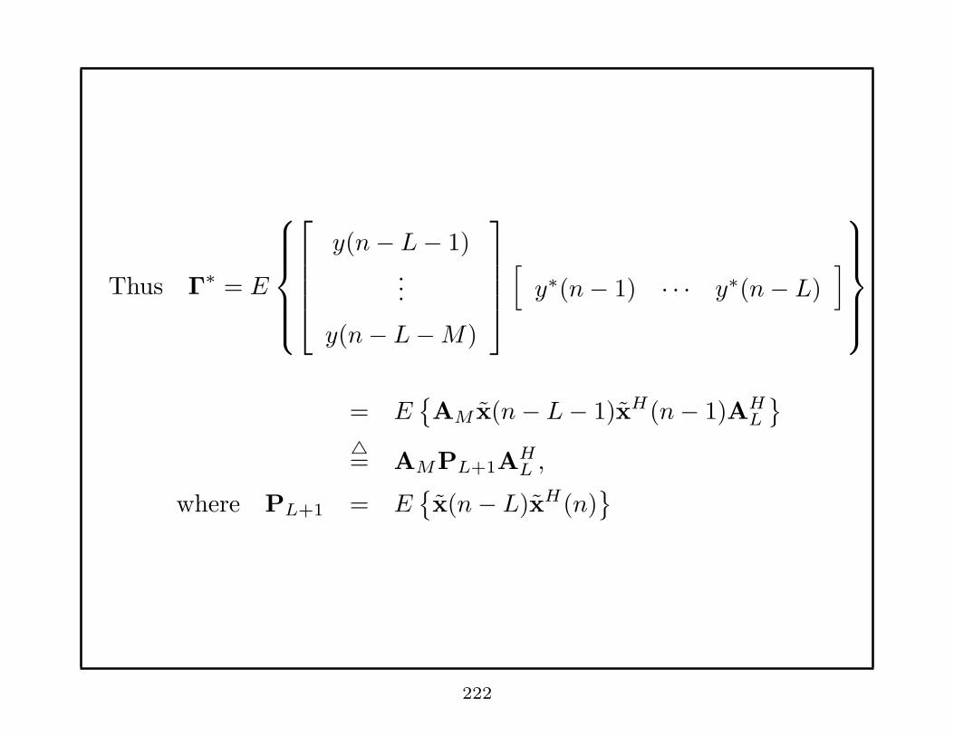
Thus Γ∗ = E
y(n− L− 1)...
y(n− L−M)
[
y∗(n− 1) · · · y∗(n− L)]
= E{AM x(n− L− 1)xH(n− 1)AH
L
}
△= AMPL+1A
HL ,
where PL+1 = E{x(n− L)xH(n)
}
222
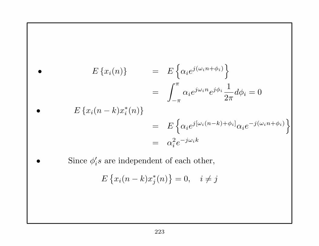
• E {xi(n)} = E{
αiej(ωin+φi)
}
=
∫ π
−π
αiejωinejφi
1
2πdφi = 0
• E {xi(n− k)x∗i (n)}
= E{
αiej[ωi(n−k)+φi]αie
−j(ωin+φi)}
= α2i e
−jωik
• Since φ′is are independent of each other,
E{xi(n− k)x∗
j (n)}
= 0, i 6= j
223
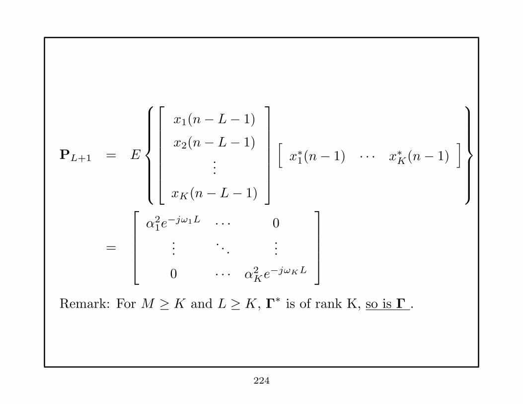
PL+1 = E
x1(n− L− 1)
x2(n− L− 1)...
xK(n− L− 1)
[
x∗1(n− 1) · · · x∗
K(n− 1)]
=
α21e
−jω1L · · · 0...
. . ....
0 · · · α2Ke
−jωKL
Remark: For M ≥ K and L ≥ K, Γ∗ is of rank K, so is Γ .
224

Consider
ryy(L) · · · ryy(1)...
ryy(L+M − 1) · · · ryy(M)
a1
...
aL
≈ −
ryy(L+ 1)...
ryy(L+M)
⇒ Γa ≈ −γ.
Remarks: rank (Γ) = min(M,L)
almost surely, due to errors in ryy(i)
• For large N , ryy(i) ≈ ryy(i) makes Γ ill conditioned.
• For large N , LS estimates of a1, · · · , aL give poor estimates of
ω1, · · · , ωK .
225

Let us use this rank information as follows: Let
Γ = UΣVH
= [U1 U2]
Σ1 0
0 Σ2
VH
1
VH2
K
L−K
denote the singular value decomposition (SVD) of Γ. (Diagonal
elements in
Σ1 0
0 Σ2
arranged from large to small ).
Since Γ is close to rank K, and Γ has rank K,
ΓK = U1Σ1VH1
(The best Rank - K Approximation of Γ in the Frobenius Norm
sense) is generally a better estimate of Γ than Γ.
ΓK a ≈ −γ, ˆa = −V1Σ−11 UH
1 γ (∗∗)
226
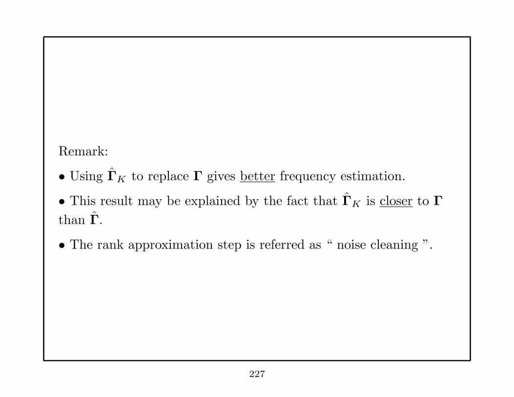
Remark:
• Using ΓK to replace Γ gives better frequency estimation.
• This result may be explained by the fact that ΓK is closer to Γ
than Γ.
• The rank approximation step is referred as “ noise cleaning ”.
227

Summary of HOYW Frequency Estimator
Step 1: Compute r(k), k = 1, 2, · · · , L+M .
Step 2: Compute the SVD of Γ and determine ˆa with (**)
Step 3: Compute the roots of
1 + ˆa1z−1 + · · ·+ ˆaLz
−L = 0
Pick the K roots that are nearest the unit circle and obtain the
frequency estimates as the angular positions (phases) of these roots.
Remarks: • Rule of Thumb for selecting L and M :
L ≈M
L+M ≈ N
3• Although one cannot guarantee that the K roots nearest the unit
circle give the best frequency estimates, empirical evidence shows
that this is true most often .
228
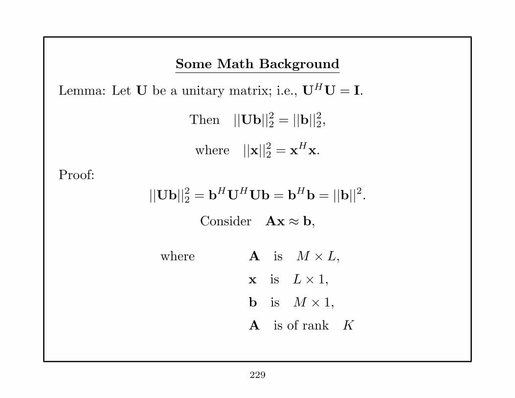
Some Math Background
Lemma: Let U be a unitary matrix; i.e., UHU = I.
Then ||Ub||22 = ||b||22,
where ||x||22 = xHx.
Proof:
||Ub||22 = bHUHUb = bHb = ||b||2.
Consider Ax ≈ b,
where A is M × L,x is L× 1,
b is M × 1,
A is of rank K
229
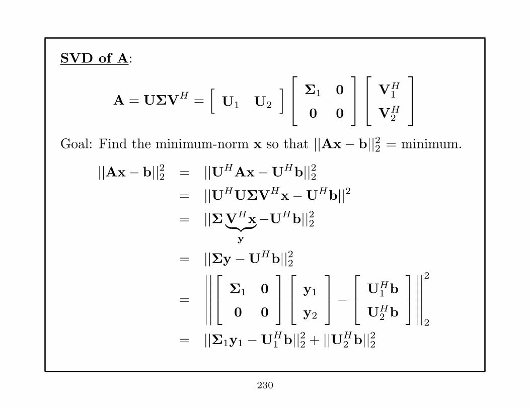
SVD of A:
A = UΣVH =[
U1 U2
]
Σ1 0
0 0
VH
1
VH2
Goal: Find the minimum-norm x so that ||Ax− b||22 = minimum.
||Ax− b||22 = ||UHAx−UHb||22= ||UHUΣVHx−UHb||2
= ||ΣVHx︸ ︷︷ ︸
y
−UHb||22
= ||Σy −UHb||22
=
∣∣∣∣∣∣
∣∣∣∣∣∣
Σ1 0
0 0
y1
y2
−
UH
1 b
UH2 b
∣∣∣∣∣∣
∣∣∣∣∣∣
2
2
= ||Σ1y1 −UH1 b||22 + ||UH
2 b||22
230

To minimize ||Ax− b||22, we must have,
Σ1y1 = UH1 b
⇒ y1 = Σ−11 UH
1 b .
Note that y2 can be anything and ||Ax− b||22 is not affected.
Let y2 = 0 so that ||y||22= ||x||22 = minimum.
⇒ VHx = y =
y1
0
⇒ x = Vy =[
V1 V2
]
y1
0
= V1y1
⇒ x = V1Σ−11 UH
1 b.
||x||22 = ||y||22 = minimum
231

SVD Prony Method
Recall:(1 + a1z
−1 + · · ·+ aLz−L)y(n)
= (1 + a1z−1 + · · ·+ aLz
−L)w(n). (L ≥ K)
At not too low SNR,
[
y(n) y(n− 1) · · · y(n− L)]
1
a1
...
aL
≈ 0
y(L) y(L− 1) · · · y(0)
y(L+ 1) y(L) · · · y(1)...
y(N − 1) y(N − 2) · · · y(N − L− 1)
1
a1
...
aL
≈ 0 (∗)
232
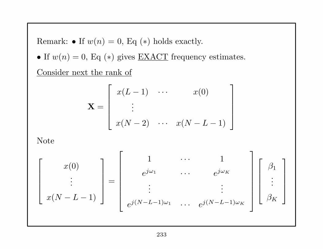
Remark: • If w(n) = 0, Eq (∗) holds exactly.
• If w(n) = 0, Eq (∗) gives EXACT frequency estimates.
Consider next the rank of
X =
x(L− 1) · · · x(0)...
x(N − 2) · · · x(N − L− 1)
Note
x(0)...
x(N − L− 1)
=
1 · · · 1
ejω1 · · · ejωK
......
ej(N−L−1)ω1 · · · ej(N−L−1)ωK
β1
...
βK
233

x(1)...
x(N − L)
=
1 .. 1
ejω1 .. ejωK
......
ej(N−L−1)ω1 .. ej(N−L−1)ωK
β1ejω1
...
βKejωK
⇒ X =
1 · · · 1
ejω1 · · · ejωK
......
ej(N−L−1)ω1 · · · ej(N−L−1)ωK
β1 0
. . .
0 βK
ej(L−1)ω1 · · · ejω1 1
ej(L−1)ω2 · · · ejω2 1...
......
ej(L−1)ωK · · · ejωK 1
234
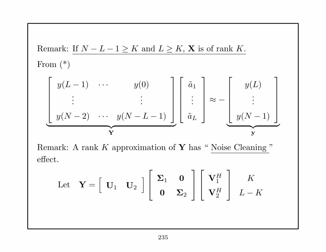
Remark: If N − L− 1 ≥ K and L ≥ K, X is of rank K.
From (*)
y(L− 1) · · · y(0)...
...
y(N − 2) · · · y(N − L− 1)
︸ ︷︷ ︸
Y
a1
...
aL
≈ −
y(L)...
y(N − 1)
︸ ︷︷ ︸
y
Remark: A rank K approximation of Y has “ Noise Cleaning ”
effect.
Let Y =[
U1 U2
]
Σ1 0
0 Σ2
VH
1
VH2
K
L−K
235
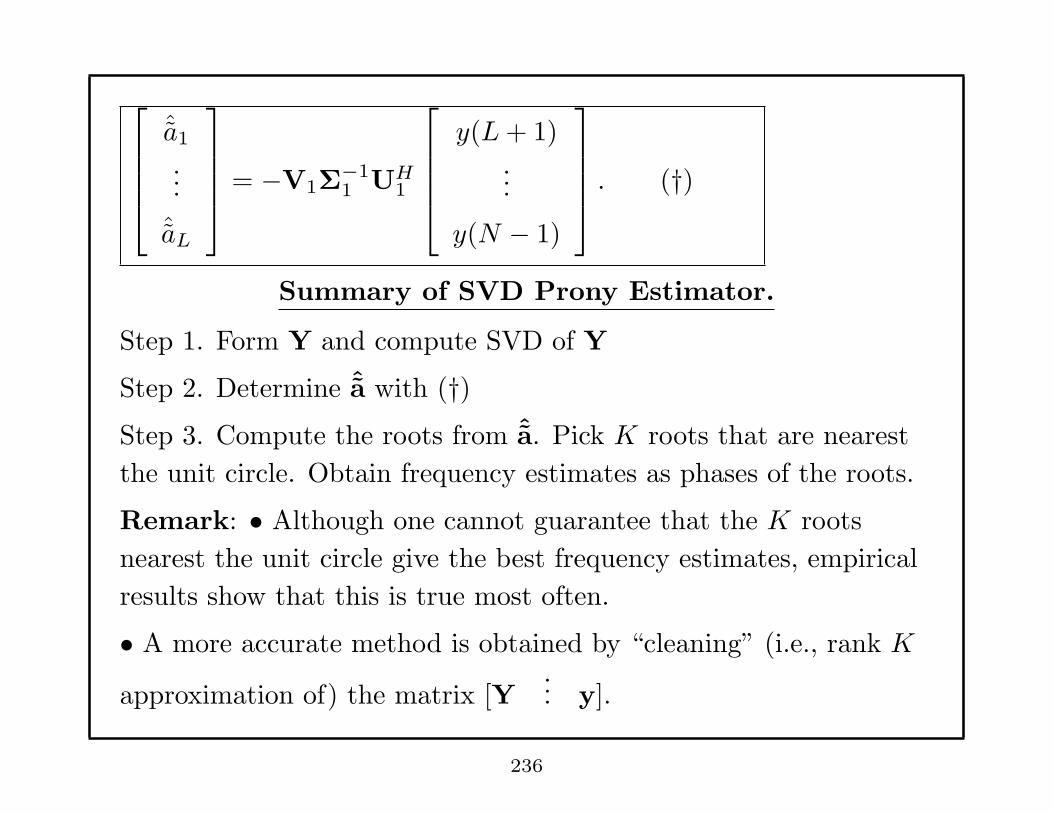
ˆa1
...
ˆaL
= −V1Σ−11 UH
1
y(L+ 1)...
y(N − 1)
. (†)
Summary of SVD Prony Estimator.
Step 1. Form Y and compute SVD of Y
Step 2. Determine ˆa with (†)Step 3. Compute the roots from ˆa. Pick K roots that are nearest
the unit circle. Obtain frequency estimates as phases of the roots.
Remark: • Although one cannot guarantee that the K roots
nearest the unit circle give the best frequency estimates, empirical
results show that this is true most often.
• A more accurate method is obtained by “cleaning” (i.e., rank K
approximation of) the matrix [Y... y].
236
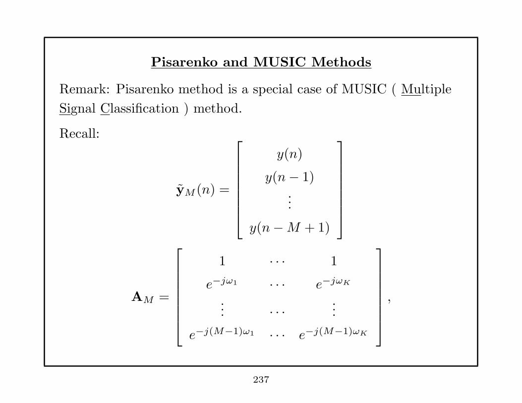
Pisarenko and MUSIC Methods
Remark: Pisarenko method is a special case of MUSIC ( Multiple
Signal Classification ) method.
Recall:
yM (n) =
y(n)
y(n− 1)...
y(n−M + 1)
AM =
1 · · · 1
e−jω1 · · · e−jωK
... · · ·...
e−j(M−1)ω1 · · · e−j(M−1)ωK
,
237

x(n) =
x1(n)...
xK(n)
,
wM (n) =
w(n)...
w(n−M + 1)
yM (n) = AM x(n) + wM (n)
Let R = E{yM (n)yH
M (n)}
= E{AM x(n)xH(n)AH
M
}
+ E{wM (n)wH
M (n)}
238

⇒
R = AMPAHM + σ2I,
P =
α21 0
. . .
0 α2K
.
Remarks: • rank (AMPAHM ) = K if M ≥ K.
• If M ≥ K,AMPAHM has K positive eigenvalues and M −K zero
eigenvalues. We shall consider M ≥ K below.
• Let the positive eigenvalues of AMPAHM be denoted
λ1 ≥ λ2 ≥ · · · ≥ λK
The eigenvalues of R are:
Two groups
λk = λk + σ2, k = 1, · · · ,K.λk = σ2, k = K + 1, · · · ,M
239

Let s1, · · · , sK be the eigenvectors of R that correspond to
λ1, · · · , λK .
Let S = [s1, · · · , sK ]
Let sK+1, · · · , sM be the eigenvectors of R that correspond to
λK+1, · · · , λM .
Let G = [sK+1, · · · , sM ]
RG = G
σ2 0
. . .
0 · · · σ2
= σ2G
RG =(
AMPAHM + σ2I
)
G
= AMPAHMG + σ2G
⇒ AMPAHMG = 0 ⇒ AH
MG = 0
240
Remark:
Let the linearly independent K columns of AM define
K -dimensional signal subspace
* Then the eigenvectors of R that correspond to the M −Ksmallest eigenvalues are orthogonal to the signal subspace.
* The eigenvectors of R that correspond to the K largest
eigenvalues of R span the same signal subspace as AM .
⇒ AM = SC for a K ×K non-singular C.
241
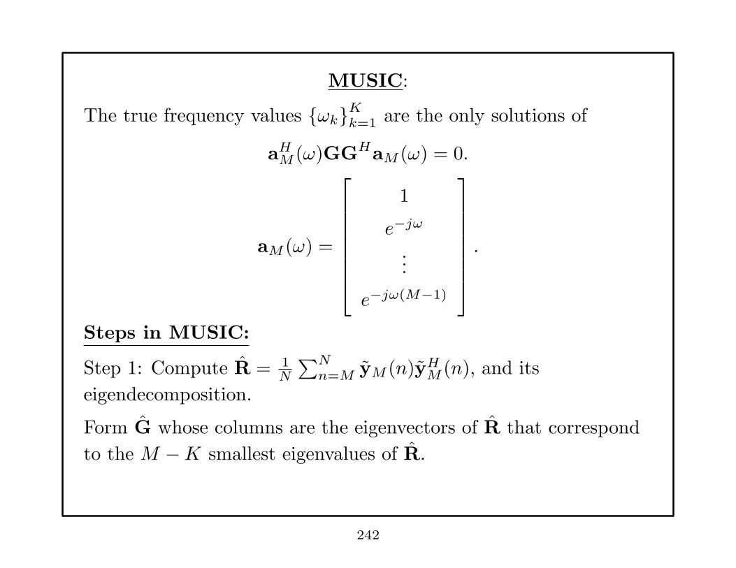
MUSIC:
The true frequency values {ωk}Kk=1 are the only solutions of
aHM (ω)GGHaM (ω) = 0.
aM (ω) =
1
e−jω
...
e−jω(M−1)
.
Steps in MUSIC:
Step 1: Compute R = 1N
∑Nn=M yM (n)yH
M (n), and its
eigendecomposition.
Form G whose columns are the eigenvectors of R that correspond
to the M −K smallest eigenvalues of R.
242

Step 2a (Spectral MUSIC): Determine the frequency estimates as
the locations of the K highest peaks of the MUSIC spectrum
1
aHM (ω)GGHaM (ω)
, ω ∈ [−π, π]
Step 2b (Root MUSIC): Determine the frequency estimates as
angular positions (phases) of K (pairs of reciprocal) roots of
equation
aHM
(z−1
)GGHaM (z) = 0
that are closest to the unit circle
aM (z) =[1 z−1 · · · z−M+1
]T, i.e., aM (z)|z=ejω = aM (ω)
243
Pisarenko Method = (MUSIC with M = K + 1)
Remarks:
• Pisarenko method is not as good as MUSIC.
• M in MUSIC should not be too large due to poor accuracy of
r(k) for large k.
244
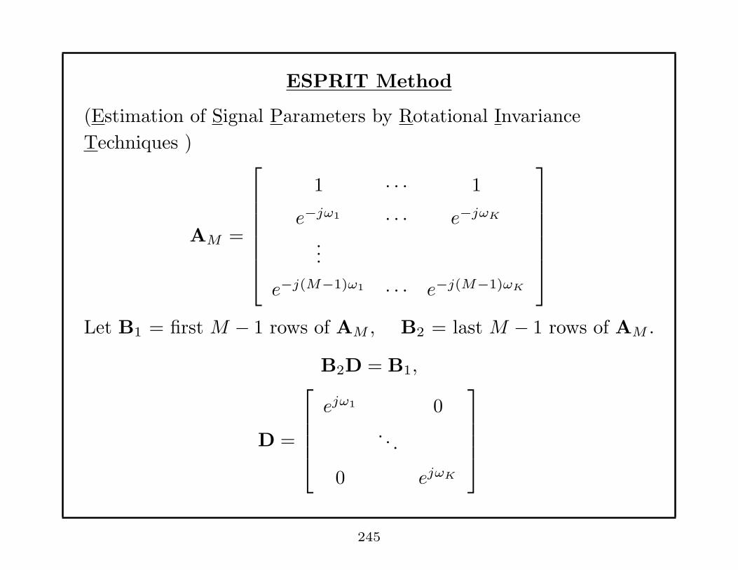
ESPRIT Method
(Estimation of Signal Parameters by Rotational Invariance
Techniques )
AM =
1 · · · 1
e−jω1 · · · e−jωK
...
e−j(M−1)ω1 · · · e−j(M−1)ωK
Let B1 = first M − 1 rows of AM , B2 = last M − 1 rows of AM .
B2D = B1,
D =
ejω1 0
. . .
0 ejωK
245
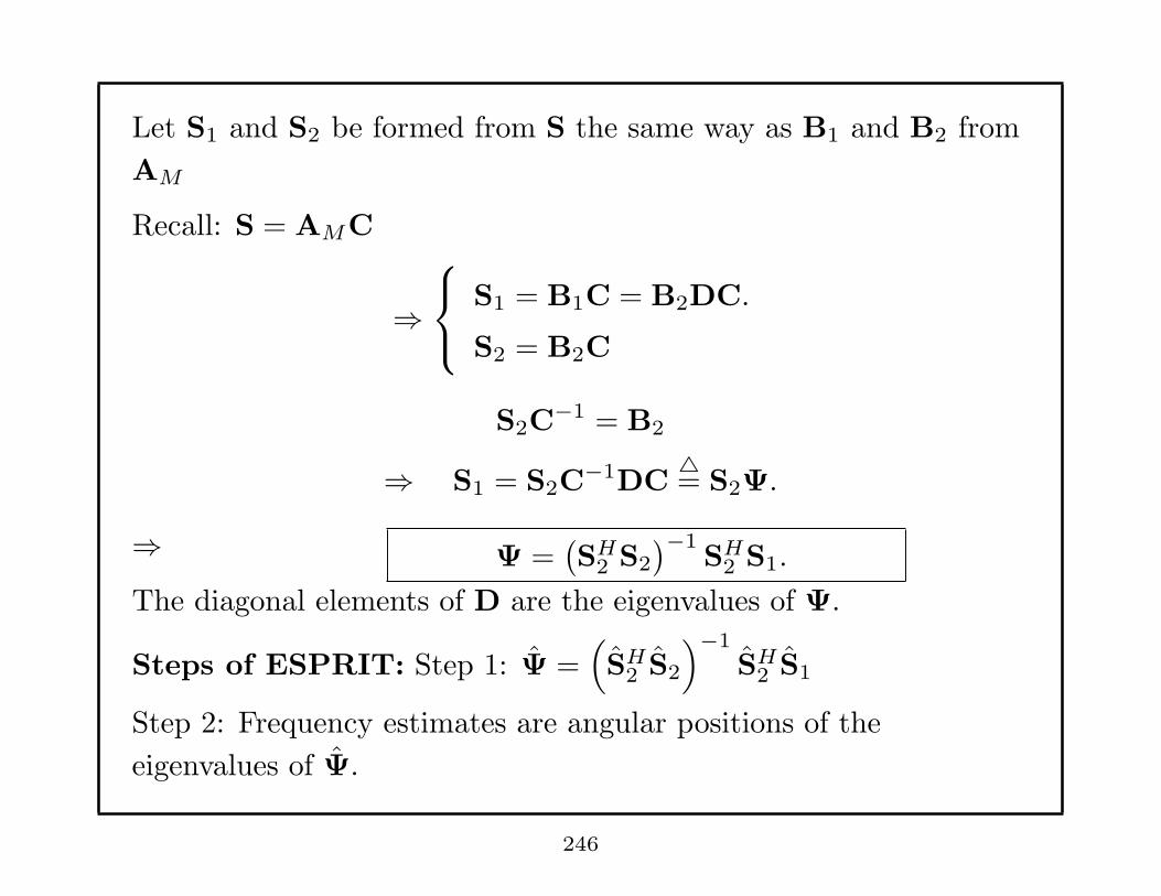
Let S1 and S2 be formed from S the same way as B1 and B2 from
AM
Recall: S = AMC
⇒
S1 = B1C = B2DC.
S2 = B2C
S2C−1 = B2
⇒ S1 = S2C−1DC
△= S2Ψ.
⇒ Ψ =(SH
2 S2
)−1SH
2 S1.
The diagonal elements of D are the eigenvalues of Ψ.
Steps of ESPRIT: Step 1: Ψ =(
SH2 S2
)−1
SH2 S1
Step 2: Frequency estimates are angular positions of the
eigenvalues of Ψ.
246

Remarks:
• S2Ψ ≈ S1
can also be solved with Total Least Squares Method
• Since Ψ is K ×K matrix, we do not need to pick K roots nearest
the unit circle, which could be wrong roots.
• ESPRIT does not require the search over parameter space, as
required by Spectral MUSIC.
All of these remarks make ESPRIT a recommended method !
247
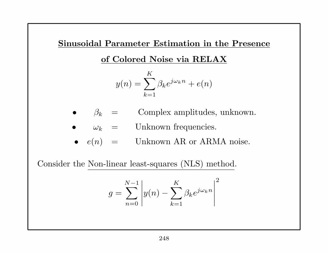
Sinusoidal Parameter Estimation in the Presence
of Colored Noise via RELAX
y(n) =
K∑
k=1
βkejωkn + e(n)
• βk = Complex amplitudes, unknown.
• ωk = Unknown frequencies.
• e(n) = Unknown AR or ARMA noise.
Consider the Non-linear least-squares (NLS) method.
g =
N−1∑
n=0
∣∣∣∣∣y(n)−
K∑
k=1
βkejωkn
∣∣∣∣∣
2
248

Remarks:
• βk and ωk, k = 1, · · · ,K are found by minimizing g .
• When e(n) is zero mean Gaussian white noise, this NLS method
is the ML method.
• When e(n) is non-white noise, NLS method gives asymptotically
(N →∞) statistically efficient estimates of ωk and βk despite the
fact that NLS is not an ML method for this case.
• The non-linear minimization is a difficult problem.
249
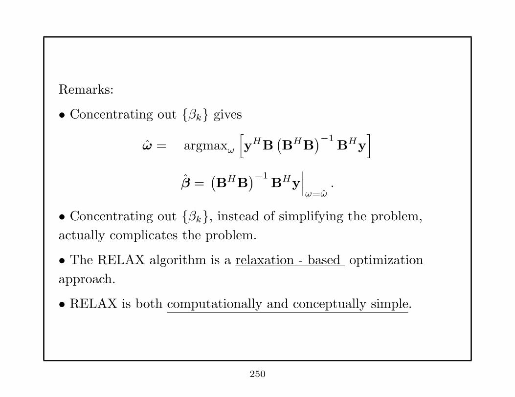
Remarks:
• Concentrating out {βk} gives
ω = argmaxω
[
yHB(BHB
)−1BHy
]
β =(BHB
)−1BHy
∣∣∣ω=ω
.
• Concentrating out {βk}, instead of simplifying the problem,
actually complicates the problem.
• The RELAX algorithm is a relaxation - based optimization
approach.
• RELAX is both computationally and conceptually simple.
250

Preparation:
Let yk(n) = y(n)−K∑
i=1,i 6=k
βiejωin
* βi and ωi, i 6= k, are assumed given, known, or estimated.
Let gk =
N−1∑
n=0
∣∣yk(n)− βke
jωkn∣∣2.
* Minimizing gk gives:
ωk = argmaxωk
∣∣∣∣∣
N−1∑
n=0
yk(n)e−jωkn
∣∣∣∣∣
2
.
βk =1
N
N−1∑
n=0
yk(n)e−jωkn
∣∣∣∣∣ωk=ωk
.
251

Remarks:
N−1∑
n=0
yk(n)e−jωkn is the DTFT of yk(n)!
(can be computed via FFT and zero-padding.)
• ωk corresponds to the peak of the Periodogram!
• βk is the peak height (complex number!) of the DTFT of yk(n)
(at ωk ) divided by N .
252

The RELAX Algorithm
Step 1: Assume K =1. Obtain ω1 and β1 from y(n).
Step 2: Obtain y2(n) by assuming K=2 and using ω1 and β1
obtained from Step 1.
Iterate until converg.
Obtain ω2 and β2 from y2(n)
Obtain y1(n) by using ω2 and β2
and reestimate ω1 and β1 from y1(n)
Step 3: Assume K = 3.
Obtain y3(n) from ω1 ,β1, ω2, β2. Obtain ω3 and β3 from y3(n) .
Obtain y1(n) from ω2, β2, ω3, β3. Reestimate ω1 and β1 from y1(n).
Obtain y2(n) from ω1, β1, ω3, β3. Reestimate ω2 and β2 from y2(n).
Iterate until g does not decrease “significantly” anymore !
253
Step 4: Assume K = 4, · · ·...
Continue until K is large enough!
Remark:
• RELAX is found to perform better than existing
high-resolution algorithms, especially in obtaining better βk,
k = 1, · · · ,K• RELAX is more robust to the choice of K and the data model
errors.
254
Top Related