


Languages
Pages
Legal


© S.J. Luck ERP Boot Camp All rights reserved
ERP Boot Camp: Data Analysis Tutorials (for use with BrainVision Analyzer-2 Software)
Preparation of these tutorials was made possible by NIH grant R25MH080794
Emily S. Kappenman, Marissa L. Gamble, and Steven J. Luck
Center for Mind & Brain and Department of Psychology
University of California, Davis Contact information for corresponding author: Emily S. Kappenman UC-Davis Center for Mind & Brain 267 Cousteau Place Davis, CA 95618 [email protected] 530-297-4425 (phone) 530-297-4400 (fax)

© S.J. Luck ERP Boot Camp All rights reserved Activity 1
1
Activity 1
Learning the Boot Camp Data Analysis Software
Learning Brain Vision Analyzer In the first activity we will overview the basic structure of the Analyzer program, including how to navigate the workspace. There are many features available in Brain Vision Analyzer, but due to time constraints we are only going to review the basic features that are most applicable to the boot camp lectures. You are welcome to work on your own to explore the additional features of Analyzer that we will not cover. To explore these options or for all of your general questions about Analyzer, we have provided the Analyzer manual at: C:\Bootcamp_Analyzer2\Documentation\Analyzer.pdf Workspace Analyzer uses workspaces to keep track of files and analysis steps. Typically, you would create a separate workspace for each experiment you conduct. We have already created a workspace for you with the raw files we will be using for the demos. Launch the Analyzer2 program by double clicking on the Vision Analyzer icon on the desktop. To load the workspace we created, go to File > Workspace > Open and click on Bootcamp_Analyzer2.wksp (located in C:\Bootcamp_Analyzer2). On the far left side of the screen is a list of the main files in the workspace. You should see four items listed, each with a name and an icon that looks like a little book. The first one labeled AnalyzerIntro can be used for this section. Analyzer adds new nodes under the original node for each step in the analysis to create a “tree” of nodes. In order to expand the tree for a particular item, click on the + sign next to the icon. You can also expand the tree by right clicking and selecting Expand All. Do this now for the AnalyzerIntro tree. You should see a number of nodes that we will now take you through. Your workspace should look like this:
. First let’s make sure that we are viewing the data in the same way. We are a positive-up lab. To properly compare the work that you do and the pictures you see in this manual, you need to have the same polarity configuration. To check the polarity, go to File > Configuration > Preferences and click on the Scaling tab. Make sure the box that says Polarity Positive Down is unchecked.
© S.J. Luck ERP Boot Camp All rights reserved Activity 1
2
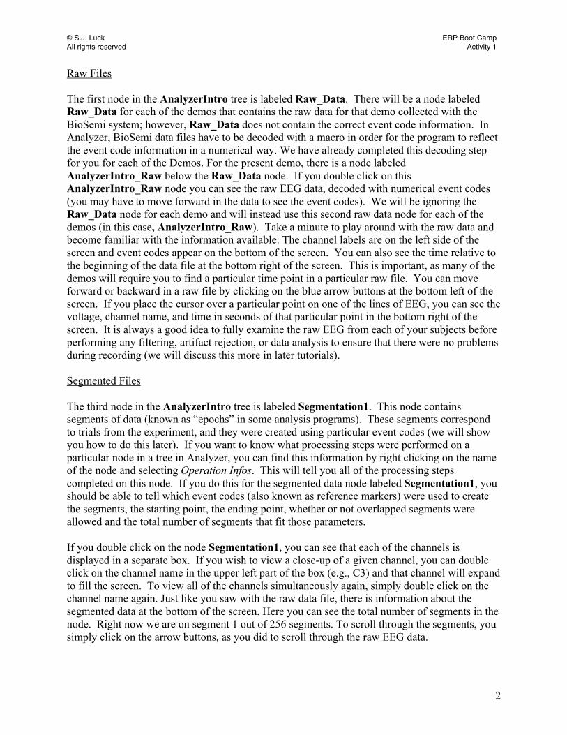
Raw Files The first node in the AnalyzerIntro tree is labeled Raw_Data. There will be a node labeled Raw_Data for each of the demos that contains the raw data for that demo collected with the BioSemi system; however, Raw_Data does not contain the correct event code information. In Analyzer, BioSemi data files have to be decoded with a macro in order for the program to reflect the event code information in a numerical way. We have already completed this decoding step for you for each of the Demos. For the present demo, there is a node labeled AnalyzerIntro_Raw below the Raw_Data node. If you double click on this AnalyzerIntro_Raw node you can see the raw EEG data, decoded with numerical event codes (you may have to move forward in the data to see the event codes). We will be ignoring the Raw_Data node for each demo and will instead use this second raw data node for each of the demos (in this case, AnalyzerIntro_Raw). Take a minute to play around with the raw data and become familiar with the information available. The channel labels are on the left side of the screen and event codes appear on the bottom of the screen. You can also see the time relative to the beginning of the data file at the bottom right of the screen. This is important, as many of the demos will require you to find a particular time point in a particular raw file. You can move forward or backward in a raw file by clicking on the blue arrow buttons at the bottom left of the screen. If you place the cursor over a particular point on one of the lines of EEG, you can see the voltage, channel name, and time in seconds of that particular point in the bottom right of the screen. It is always a good idea to fully examine the raw EEG from each of your subjects before performing any filtering, artifact rejection, or data analysis to ensure that there were no problems during recording (we will discuss this more in later tutorials). Segmented Files The third node in the AnalyzerIntro tree is labeled Segmentation1. This node contains segments of data (known as “epochs” in some analysis programs). These segments correspond to trials from the experiment, and they were created using particular event codes (we will show you how to do this later). If you want to know what processing steps were performed on a particular node in a tree in Analyzer, you can find this information by right clicking on the name of the node and selecting Operation Infos. This will tell you all of the processing steps completed on this node. If you do this for the segmented data node labeled Segmentation1, you should be able to tell which event codes (also known as reference markers) were used to create the segments, the starting point, the ending point, whether or not overlapped segments were allowed and the total number of segments that fit those parameters. If you double click on the node Segmentation1, you can see that each of the channels is displayed in a separate box. If you wish to view a close-up of a given channel, you can double click on the channel name in the upper left part of the box (e.g., C3) and that channel will expand to fill the screen. To view all of the channels simultaneously again, simply double click on the channel name again. Just like you saw with the raw data file, there is information about the segmented data at the bottom of the screen. Here you can see the total number of segments in the node. Right now we are on segment 1 out of 256 segments. To scroll through the segments, you simply click on the arrow buttons, as you did to scroll through the raw EEG data.
© S.J. Luck ERP Boot Camp All rights reserved Activity 1
3
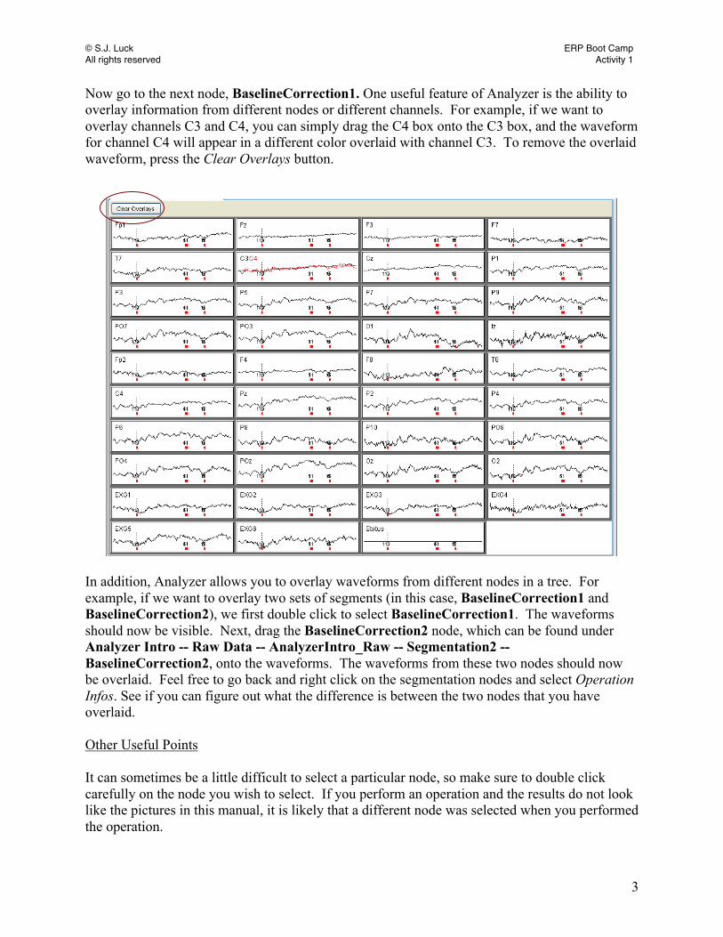
Now go to the next node, BaselineCorrection1. One useful feature of Analyzer is the ability to overlay information from different nodes or different channels. For example, if we want to overlay channels C3 and C4, you can simply drag the C4 box onto the C3 box, and the waveform for channel C4 will appear in a different color overlaid with channel C3. To remove the overlaid waveform, press the Clear Overlays button.
In addition, Analyzer allows you to overlay waveforms from different nodes in a tree. For example, if we want to overlay two sets of segments (in this case, BaselineCorrection1 and BaselineCorrection2), we first double click to select BaselineCorrection1. The waveforms should now be visible. Next, drag the BaselineCorrection2 node, which can be found under Analyzer Intro -- Raw Data -- AnalyzerIntro_Raw -- Segmentation2 -- BaselineCorrection2, onto the waveforms. The waveforms from these two nodes should now be overlaid. Feel free to go back and right click on the segmentation nodes and select Operation Infos. See if you can figure out what the difference is between the two nodes that you have overlaid. Other Useful Points It can sometimes be a little difficult to select a particular node, so make sure to double click carefully on the node you wish to select. If you perform an operation and the results do not look like the pictures in this manual, it is likely that a different node was selected when you performed the operation.

© S.J. Luck ERP Boot Camp All rights reserved Activity 1
4
If this happens or you make another type of error or wish to delete a step in the analysis tree, you can simply right click on the n2de and select Delete. Let’s try this now. Delete the BaselineCorrection2 node by right clicking and selecting Delete. Now let’s recreate the node we just deleted. In other words, let’s create a baseline correction node for Segmentation2, so that we have the same analysis steps for Segmentation1 and Segmentation2. Analyzer allows you to duplicate operations performed on one node on a second node very easily. This allows you to save a lot of time if you are analyzing multiple subjects or data sets. To do this, simply drag the node that has the operation you want to duplicate onto the node on which you want to perform the operation. For example, to perform the baseline correction we did for Segmentation1 on Segmentation2, we simply drag the BaselineCorrection1 node onto the Segmentation2 node. Do this now. Analyzer performs the operation from the first node on the second node for us. In addition, if there had been subsequent steps after baseline correction, it would have performed all of those as well. Just make sure to rename the new nodes to keep track of them. For example, Analyzer named the new baseline correction node you created, BaselineCorrection1. You should rename this node BaselineCorrection2 by right clicking and selecting Rename, or by clicking once on the name, pausing, and clicking a second time. Most of the activities in this tutorial will require that you use some type of transformation. These can be found underneath the Transformations tab the top of the Analyzer window. The transformations are then grouped into Dataset Preprocessing, Artifact Rejection/Reduction, Frequency and Component Analysis, Segment Analysis Functions, Comparison and Statistics, Special Signal Processing, and Others. You may need to click on another button underneath these initial function class buttons to see more options. If you see a little arrow ∨, it indicates that more options can be seen if you click on that transformation. As described above, overlaying data is a great feature of Analyzer that really allows you to inspect your data. However, you may find that sometimes if you try to overlay certain types of data, you are unable to see both sets of data in the window. This occurs whenever the offsets of the data are drastically different and the scaling does not allow both sets of data to be visible at the same time. For instance, if you try to overlay segments that have not been baseline corrected or if you overlay data with different high-pass filter cutoffs, the differences in the offsets of the data may make it hard to see the original and overlaid data simultaneously. In such cases, you can view the data by using the Windows > Tile Horizontal or Tile Vertical options to do side-by-side comparisons.

© S.J. Luck ERP Boot Camp All rights reserved Activity 2
1
Activity 2
Re-referencing For this next tutorial you will be using the Demo1 tree. The data in this demo are from the Monster paradigm used during the data collection activity and discussed in the Boot Camp lecture. There will also be a description of the Monster paradigm and an explanation of the event code scheme in later tutorials. To view the first raw EEG file, double click on the Demo1_Raw node. If you do not see Demo1_Raw listed under the Demo1 file header, press the + next to Demo1, which should produce a file called Raw Data. Press the + next to Raw Data and this should expose the Demo1_Raw node. Notice that you have 38 EEG channels. If you cannot see
all 38 EEG channels, click on the button until all channels are visible. The 38 channels include 32 EEG scalp sites labeled with the corresponding 10-20 electrode system label (FP1, Fz, etc.) and six external electrodes labeled EXG1-EXG6. EXG1-EXG6 correspond to the following positions:
EXG1- Horizontal EOG Right (HEOG_R) EXG2- Horizontal EOG Left (HEOG_L) EXG3- Vertical EOG Lower (VEOG_Lower) EXG4- Vertical EOG Upper (VEOG_Upper) EXG5- Left Mastoid (LM) EXG6- Right Mastoid (RM)
Once you have examined the raw EEG data, you are ready to start processing the data. Remember, it is always a good idea to thoroughly examine the raw EEG data from each subject before beginning data analysis. This allows you to identify any weird artifacts or segments of data that need to be excluded. This is especially important for re-referencing the data, because any artifacts present in the reference channels will be propagated to all of your channels when you re-reference the data. Our first goal in this activity will be to re-reference the EEG channels to the average of the left and right mastoid channels. Our second goal will be to create a bipolar HEOG channel (HEOG_R minus HEOG_L) and a bipolar VEOG channel (VEOG_Lower minus VEOG_Upper). Creating bipolar channels for the EOG signals will help in the identification of eyeblink and eye movement artifacts, as you will see in the Artifact Rejection tutorial. The data files we will be using throughout these demos were collected with the Biosemi Active-Two system. Unlike traditional EEG systems that record data in a differential mode, the Biosemi system records in what is known as single-ended mode. This means that each site is recorded as the potential between that site and the common mode sense (CMS) electrode site (which is analogous to a ground electrode). Conventional systems record the potential between an active site and the ground electrode and the voltage between a reference site and a ground electrode, and then electronically form the difference between the active and reference sites online. With the Biosemi system we perform this subtraction offline during data analysis. First let’s re-reference the data recorded in single-ended mode. Later we will discuss how to re-reference data collected in differential mode.

© S.J. Luck ERP Boot Camp All rights reserved Activity 2
2
Double-click on the Demo1_Raw file. To re-reference the data, select Transformations > Dataset Preprocessing > Linear Derivation. The Linear Derivation command is used to create new EEG channels that are linear (summed and scaled) combinations of the existing EEG channels. However, this way of referencing data can be prone to mistakes and can be rather tedious to set up, particularly if you are using a dataset with many channels. However, manually creating re-referenced data using the linear derivation tool is a great exercise to show precisely what is being done to the data during re-referencing. Therefore, we will work through the logic of re-referencing our data for one channel of EEG using the linear derivation tool to work through the math involved. Let’s do this for the FP1 channel. Click on the button Load from File, and when it prompts you for the text file, load C:\Bootcamp_Analyzer2\workfiles\Reference_FP1_sem.txt. The file should look like this:
Notice that the leftmost column of the spreadsheet contains the names of the output channels (i.e., the channels that we will create). The top row contains the names of the input channels (i.e., the original channels from the demo1_Raw file). Each cell in the matrix contains a number that indicates the scaling of the input channel that will be used in computing the output channel. In this case, we are re-referencing channel FP1 to the average of the left and right mastoids. Most of the values in the matrix are set to 0, but if you look closely you will see a 1 wherever a particular electrode site in the input channel column is also present in the output channel column, in this case channel FP1. In the EXG5 and EXG6 columns (which represent the left mastoid and right mastoid, respectively), you will see that each of these columns has a coefficient of -0.5. Let’s work through the logic of this. Originally, the FP1 electrode site was recorded in single-

© S.J. Luck ERP Boot Camp All rights reserved Activity 2
3
ended mode as the potential between FP1 and CMS. Now we want to re-reference FP1 to the left and right mastoids by subtracting the average of channels EXG5 and EXG6 from channel FP1. Thus, we want to compute the following: FP1referenced = FP1 original – [(EXG5 + EXG6) ÷ 2] which is the same as: FP1 referenced = FP1 original+ (-0.5 x EXG5) + (-0.5 x EXG6) Click OK and a new node will appear under Demo1_raw labeled Linear Derivation. Re-label this new node Demo1_FP1_sem. FP1 has now been re-referenced to the average of the two mastoids (i.e. EXG5 and EXG6). Of course, we need to re-reference all of our data channels and not just FP1. Now that we understand how re-referencing works, instead of doing this using the linear derivation method for each channel of data, we will re-reference the entire data set in one step with the re-referencing option in Analyzer. Let’s go back to our original unreferenced raw EEG data, node Demo1_Raw. Go to Transformations > Dataset Preprocessing > Channel Preprocessing > New Reference. The window should look like this:
© S.J. Luck ERP Boot Camp All rights reserved Activity 2
4
Select the two mastoid channels (EXG5 and EXG6). You will see that there is a checkbox for whether to include an implicit reference into the calculation of the new reference. The Include Implicit Reference into Calculation of the New Reference button should be unchecked for re-referencing data collected in single-ended mode, because there is no real implicit reference channel. Click Next. In the next window you need to indicate the channels to which you would like the new reference to be applied. We will re-reference all 32 of the EEG data channels, but we will not re-reference the external eye or mastoid channels or the Status channel (which contains the event code information). Click Next. It will then ask you the name of the new channel (leave this blank). Click Finish and a new node will be created named New Reference. Rename this node to Demo1_ref_sem. Now we have re-referenced the EEG data channels. Before we create the bipolar EOG channels, let’s work through the logic of re-referencing for data collected in differential mode, which many of you may be using in your own labs. Re-referencing Data in Differential Mode Unlike the Biosemi system, most systems record the data online as referenced to a specific site, like a mastoid, an earlobe, or the nose. If the data are originally collected with a reference on one side of the head (like a mastoid or earlobe), it is usually desirable to re-reference the data offline to the average of sites over both sides of the head (e.g., to the average of the left and right mastoids). This is conceptually the same as the process we just completed in which we re-referenced offline to the average of the two mastoids, but we need to take into account that the data are already referenced to one of the mastoids. How exactly does this work? Let’s imagine that we collected our data online referenced to the left mastoid. This means that each of our data channels and the right mastoid were all collected as the difference between the data channel and the left mastoid. For the Fp1 site, for example, this is literally equal to Fp1 – Left Mastoid. Now we want to re-reference our data so that each channel is re-referenced to the average of the two mastoids. If you work through the algebra, it turns out that in order to re-reference our data to the average of the left and right mastoids, you simply need to subtract out half of the right mastoid. If you would like to work through this algebraically, the equations can be found on page 108 of Luck, 2005 or in your boot camp lecture notes. To see how this works, go to Transformations > Dataset Preprocessing > Linear Derivation and load the text file C:\Bootcamp_Analyzer2\workfiles\Reference_FP1_dm.txt. You can see that for the new channel FP1 there is a -0.5 for EXG6 (right mastoid) and a 1 for FP1 just like we had for the data collected in single-ended mode. However, because in this example the data were collected (hypothetically) as referenced to the left mastoid online, there is a zero in the EXG5 spot (remember, the data were already collected against this reference online, hypothetically).
© S.J. Luck ERP Boot Camp All rights reserved Activity 2
5
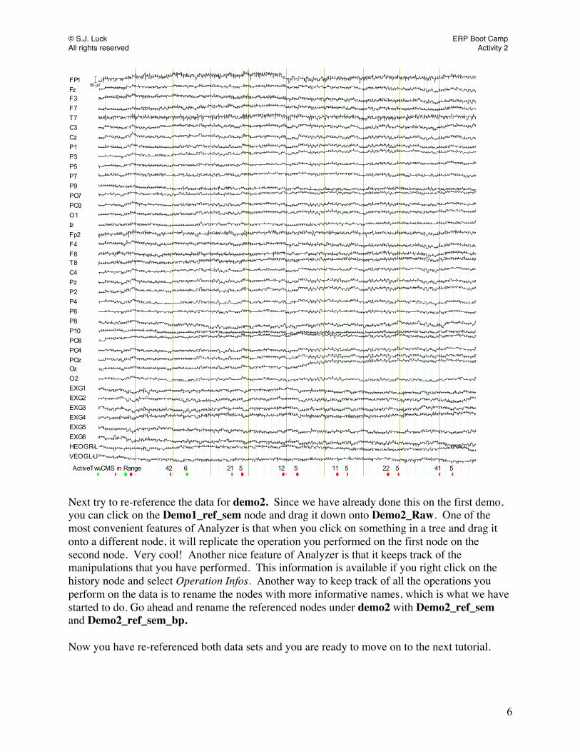
With this derivation we will end up with FP1 re-referenced to the average of the right and left mastoid. Once again, we can do this for all of our EEG channels in one step using the re-referencing tool in Analyzer (feel free to hit Cancel on the linear derivation for FP1). Make sure that you have selected the unreferenced raw data, Demo1_Raw, and then go to Transformations > Dataset Preprocessing > Channel Preprocessing > New Reference. This time you will just select the right mastoid as a reference (EXG6). You will also need to make sure that you DO check the box for including an implicit reference into the calculation of the new reference, since these data were (hypothetically) referenced online to the left mastoid. Checking this box means that Analyzer will subtract out half of EXG5 from the EEG channels to which you choose to apply the selected reference. Leaving this box unchecked would mean that Analyzer would subtract out the entire channel from each of the selected EEG channels, and that would not result in an average mastoid reference. Again, we will re-reference all 32 of the EEG data channels. Rename the new node to Demo1_ref_dm. Bipolar channels In addition to referencing the scalp sites to the average of the mastoids, you may also want to create bipolar channels from the ocular electrodes. We will discuss the usefulness of these bipolar channels more in the tutorial on artifact rejection. Double click on Demo1_ref_sem and select Transformations > Dataset Preprocessing > Linear Derivation and load file C:\Bootcamp_Analyzer2\workfiles\Bipolar.txt. If you scroll down to the bottom of the Linear Derivations window, you will see a channel labeled HEOGR-L, which is created by taking channel EXG1 minus channel EXG2 (HEOG_R minus HEOG_L). This will create a bipolar channel. By creating a channel like this, all of the EEG that is the same at the two HEOG sites will be subtracted away, making it easier to see the horizontal eye movements, which are opposite in polarity at the HEOG_L and HEOG_R sites (this will become more important later on in the tutorials). In addition to the bipolar HEOG channel, we have also created a bipolar VEOG channel (VEOGL-U). This channel is the subtraction of VEOG_Lower minus VEOG-Upper (EXG3 minus EXG4). This subtracts away all of the brain activity in common to these two sites, leaving only the difference (which is large for blinks, which are opposite in polarity below versus above the eyes). Click OK and a new node will appear under the Demo1_ref_sem labeled Linear Derivation. Rename this new node Demo1_ref_sem_bp. The re-referenced data should look like the screen shot below:
© S.J. Luck ERP Boot Camp All rights reserved Activity 2
6
FP1FzF3F7T7C3CzP1P3P5P7P9PO7PO3O1IzFp2F4F8T8C4PzP2P4P6P8P10PO8PO4POzOzO2EXG1EXG2EXG3EXG4EXG5EXG6HEOGR-LVEOGL-U
31 5 42 21 5 12 5 11 5 22 5 41 5
50 µV
CMS in RangeStart EpochActiveTwo MK2ActiveTwo MK2CMS in Range 56
Next try to re-reference the data for demo2. Since we have already done this on the first demo, you can click on the Demo1_ref_sem node and drag it down onto Demo2_Raw. One of the most convenient features of Analyzer is that when you click on something in a tree and drag it onto a different node, it will replicate the operation you performed on the first node on the second node. Very cool! Another nice feature of Analyzer is that it keeps track of the manipulations that you have performed. This information is available if you right click on the history node and select Operation Infos. Another way to keep track of all the operations you perform on the data is to rename the nodes with more informative names, which is what we have started to do. Go ahead and rename the referenced nodes under demo2 with Demo2_ref_sem and Demo2_ref_sem_bp. Now you have re-referenced both data sets and you are ready to move on to the next tutorial.
© S.J. Luck ERP Boot Camp All rights reserved Activity 3
1
Activity 3 Segmentation
The next step in our data analysis is to create segments of data corresponding to the trials in our experiment. Data segmentation, which is known as epoching in some data analysis systems, simply means chopping up the continuous EEG data into small time periods (e.g., 1000 ms). The most common way to do this is to extract segments surrounding the event codes from your experiment (e.g., from 200 ms prior to the event code until 800 ms after the event code), although there are other ways to segment data in Analyzer (e.g., creating segments at particular times, manually selecting segments, etc.). Before we segment the data, let’s review a little bit about the MONSTER experiment. In this experiment, subjects are presented with a set of stimuli on each trial, composed of a black letter (A or B) and a white letter (also A or B), with one letter on each side of fixation. Subjects are told to attend to either the white or black letter for a block of trials, counterbalancing whether the participant presses the left button for A and the right button for B or vice versa. We have also manipulated the probability of the stimuli, such that in some blocks A is 80% probable and B is 20% probable, and in other blocks B is 80% probable and A is 20% probable. In addition to the target and non-target presented on each trial, there are also black-and-white checkerboards that are presented either in the upper visual field or the lower visual field. A key element of the MONSTER paradigm is that it contains several (mostly) orthogonal experimental manipulations that allow different ERP components to be isolated by means of various difference waves. The four main components we will isolate are:
1) The C1 Wave, which comes from primary visual cortex. Due to the folding pattern of the calcarine fissure, the C1 is opposite in polarity for upper vs. lower field stimuli, with a negative voltage for the upper field and a positive voltage for the lower field. To isolate the C1 from the overlapping components, we will make an upper-minus-lower difference wave corresponding to the location of the checkerboard.
2) The lateralized readiness potential (LRP) reflects preparation of a response, and it is observed over the hemisphere contralateral to the hand being prepared. We will isolate it with a contralateral-minus-ipsilateral difference wave, relative to the response hand.
3) The P3 wave is larger for rare stimulus categories than for frequent stimulus categories, and it provides a measure of the time required to categorize a stimulus.
4) The N2pc component reflects the focusing of attention onto a lateralized target, and it is negative over the hemisphere contralateral to the target. We will isolate it with a contralateral-minus-ipsilateral difference wave, just like the LRP, but it will be contra vs. ipsi to the target side rather than the response hand.
There is actually a fifth factor in the design, which is the compatibility between the target and the nontarget on the other side of the fixation point (e.g., whether the nontarget is an A or B when the target is an A). If you have time, a good exercise would be to figure out how to isolate the effect of that factor (which might be expected to influence the N2 component over central scalp sites).

© S.J. Luck ERP Boot Camp All rights reserved Activity 3
2
The MONSTER paradigm is extremely efficient because we can collapse across all the other factors when we are examining a given component. For example, when we isolate the C1 wave, we make one average for all the trials with checkerboards in the upper visual field and another average for all the trials with checkerboards in the lower visual field, irrespective of the target side, what the target is, what the response is, etc. The same set of trials can be subdivided in several different ways to isolate different components. Although this ignores any interactions between the factors, that’s OK as a first approximation. You might want to figure out how to assess these interactions if you have time at the end (e.g., is the N2pc larger when the checkerboards are in the lower visual field?). Event Codes for the MONSTER Paradigm To make all of these orthogonal difference waves, you first need to understand the scheme we used for the event codes. The event codes created by the MATLAB program range between 1 and 255, and we will use the different digits to represent different aspects of the experimental design. If we had enough digits in the event codes, we could use a separate digit to represent each factor. Indeed, the Biosemi digitization software allows event codes up to 65536, which would make it easy to represent all of our factors in different digits. Unfortunately, most stimulus presentation systems (and EEG acquisition systems) are limited to a range of 1-255 or even 1-127. In the MONSTER paradigm, we use the digit in the hundreds place to represent whether subjects are attending to the white or black stimulus in the current trial block, with codes of 0xx for attend-black and 1xx for attend-white. We use the digit in the tens place to represent whether the target is on the left (a value of x1x ,x2x, x5x, or x6x) or on the right (a value of x3x, x4x, x7x, or x8x), and whether the checkerboards are in the upper field (x1x, x3x, x5x, or x7x) or in the lower field (x2x, x4x, x6x, x8x). In addition the tens place also indicates whether A = left response (x1x, x2x, x3x, or x4x) or A = right response (x5x, x6x, x7x, or x8x). For example, an event code of 12x means that white was attended, that the white target was on the left side, that the checkerboards were in the lower visual field and the participant should press the left button for A and press the right button for B. The digit in the ones place codes the identity of the target stimulus, the identity of the nontarget stimulus (both of which can independently be A or B), and the probability of the stimuli, as indicated by the table below: Stimulus Event Codes
Hundreds place 0 = attend black 1 = attend white Tens place 1 = left side target, upper checkerboards, A=Left Response 2 = left side target, lower checkerboards, A=Left Response 3 = right side target, upper checkerboards, A=Left Response 4 = right side target, lower checkerboards, A=Left Response 5 = left side target, upper checkerboards, A=Right Response 6 = left side target, lower checkerboards, A=Right Response 7 = right side target, upper checkerboards, A=Right Response 8 = right side target, lower checkerboards, A=Right Response

© S.J. Luck ERP Boot Camp All rights reserved Activity 3
3
Ones place 1 = A target (A is Frequent), A nontarget 2 = A target (A is Frequent), B nontarget 3 = A target (A is Rare), A nontarget 4 = A target (A is Rare), B nontarget 5 = B target (B is Frequent), A nontarget 6 = B target (B is Frequent), B nontarget 7 = B target (B is Rare), A nontarget 8 = B target (B is Rare), B nontarget
Response Event Codes Responses 5 = Left Response 6 = Right Response
For example, an event code of 137 means that subjects were attending to white, the white item was on the right side, the checkerboards were in the upper field, A = left response, the white target item was a B, which was 20% probable, and the black nontarget item was an A. Note that a left hand response produces an event code of 5 and a right hand response produces an event code of 6. Scroll through the data in Demo1_raw and make sure that you see the event codes, denoted with a vertical marker through the EEG and the event code value at the bottom of the screen. You may notice an occasional event code of 7 in the data file, which does not map on to the event codes described above. The 7s occur whenever both the left and right response buttons are pressed simultaneously. For all of our data analysis activities, you can just ignore the 7s. Segmentation Now that we know about the monster paradigm, let’s use this information to segment the data for the different ERP components of interest. Let’s start with the C1 analysis. We want to separate the data into two different types of segments: targets with checkerboards in the upper visual field and targets with checkerboards in the lower visual field. If you look at the chart above you should be able to figure out which event codes belong in the Upper segment and which belong in the Lower segment. Selecting the event codes in creating segments of data is one of the easiest places to make a mistake during ERP data analysis. Make sure to double-check the event codes you select, and look in the file: C:\Bootcamp_Analyzer2\Documentation\event codes if you want to compare your selected event codes with the appropriate event codes. This will make sure that your data match the screenshots throughout the tutorials. To create the segments for the C1 wave, select Demo1_ref_sem_bp and then go to Transformations > Segment Analysis Function > Segmentation. A box like the one below will appear. Note that Analyzer2 uses the term “marker” for event codes.

© S.J. Luck ERP Boot Camp All rights reserved Activity 3
4
Select Create new Segments based on a marker position and then press Next. Another box will appear. On the left will be the available markers (all of the event codes in the data file). This will include the response event codes, which it may label as stimulus codes, but that is ok--the software cannot make the distinction between different types of event codes. Select all of the markers that belong to the Upper C1 segments and click the Add button. This will move these markers to the right of the box under the Selected Markers area. Please note that the C:\Bootcamp_Analyzer2\Documentation\event codes file lists all possible event codes for a particular segmentation, and some of those event codes may not appear in a given data file due to the randomization of trials.

© S.J. Luck ERP Boot Camp All rights reserved Activity 3
5
Notice that there is a box in the window called Advanced Boolean Expression. In this box you can indicate other parameters for segmentation selection. For example, if we wanted to only select those segments that are followed by a left response event code (event code 5) within 1000 ms of the stimulus event code, we would put 5(200, 1000) in the Advanced Boolean Expression box. This expression simply indicates that the selected stimulus event codes in Selected Markers should only be included in the segmentation process if there was an event code 5 within 200 ms to 1000 ms following the stimulus event code. Normally we would only want to include trials with correct responses. This would actually require us to initially create two different segmentations for the Upper checkerboards. Think about why this might be. For now, however, we are going to accept all segments regardless of accuracy (although we will modify this for isolating the LRP component). Click Next to continue with segmentation. A new box will pop up that lets you specify the start and end of the segments based on either time (in ms) or data points. Select Based on Time and specify -200 ms for Start time and 800 ms for the End time. This will provide a pre-stimulus baseline period of 200 ms and a post-stimulus period of 800 ms, for a total segment length of 1000 ms. As discussed in the boot camp lectures, the prestimulus interval should be sufficiently long to assess overlapping activity from the previous trial as well as the background noise level. For some experiments, you may wish to use a prestimulus interval that is much longer than 200 ms.

© S.J. Luck ERP Boot Camp All rights reserved Activity 3
6
There are two more options in this window. The first, Allow Overlapped Segments should be checked, whereas the Skip Bad Intervals option should be unchecked. The option to allow overlapped segments just means that if one of our segments overlaps in time with the next one, we will include both segments. This actually won’t affect our results for this experiment, since there will be no overlapping segments. The skip bad intervals option rejects intervals that have been marked with artifacts. However, since we haven’t done any artifact rejection yet, this should not matter either. The box should look like the image above. Click Finish and a new node will be created called Segmentation. Rename this node Upper, to indicate that these segments correspond to trials in which the checkerboard stimuli were in the upper visual field. Go back to Demo1_ref_sem_bp and go through segmentation for the checkerboards in the lower visual field. You should be able to figure out these event codes from the information above (or check in the event codes file). Name this node Lower. Now we have the segments we need to create the C1. But first let’s create the segments we need for the LRP. Go back and double click on Demo1_ref_sem_bp. We are now going to create Right_Resp and Left_Resp segmentation files. These segments are going to be for the LRP analysis, so we are looking for those conditions where the participant responded with the right hand (correct right responses when A = Right hand and B = Right hand for the A and B stimuli, respectively) and when the subject responded with the left hand (correct left responses when A = Left hand and B = Left hand for
© S.J. Luck ERP Boot Camp All rights reserved Activity 3
7
the A and B stimuli, respectively). At this point, however, we will be time-locking to the stimulus preceding the response rather than computing response-locked averages. Figure out which event codes belong in each condition and then double check with the event codes file. For this particular segmentation, we only want to isolate the instances where the participant made the correct responses. Remember that a left hand response is indicated by an event code of 5, and a right hand response is indicated by an event code of 6. See if you can figure out the correct way to make these segmentations based on what we have learned before moving on to the next paragraph. Go to Transformations > Segment Analysis Function > Segmentation and select the appropriate markers for Left_Resp. In the Advanced Boolean Expression box type 5(200, 1000), to specify that an event code of 5 should occur within 200-1000 ms after the stimulus event code. Go ahead and create the segments for Right_Resp (remember to change the response code to 6!). Don’t forget to rename the nodes with the appropriate names. Baseline Correction We have one more step before we move on to artifact rejection. We must baseline-correct the segmented data. Baseline correction involves calculating the mean voltage over a specified window and subtracting that value from each point in the segment. By subtracting this voltage, you will remove any large voltage offsets from each segment and set a new “zero” voltage level. It is very important to keep in mind that baseline correction is a manipulation of the data and will influence every subsequent step of processing and analysis. Double click on Upper and select Transformations > Segment Analysis Functions > Baseline Correction. A small window will pop up asking for the Range for Mean Value Calculation. Enter -200 ms for the Begin, and 0 ms for the End time points. This will give you a good range for the baseline correction calculation. Press OK and rename the segment Upper_bc. Do this for the lower segments and the LRP segments as well. As we will discuss in the next tutorial, baseline correcting the segmented data allows us to identify artifacts in the data based on voltages. We have found for most of our studies that a baseline window of 200 ms prestimulus works well. However, this is dependent on the 200 ms prestimulus being relatively flat and free from noise and other artifacts. Regardless of which baseline interval you choose to use, it is a good idea to look at the data and make sure that the baseline period you have chosen is relatively flat and free from noise contamination before baseline correcting. Think about why this is so important.

© S.J. Luck ERP Boot Camp All rights reserved Activity 4
1
Activity 4 Artifacts and Averaging
Now that we have segmented the data we are ready to perform artifact rejection. Artifact rejection is a very important part of ERP data analysis, as it allows us to clean up our data to ensure that we are getting a good signal from the data we collected. But keep in mind that artifact rejection cannot save noisy data, and it is always best to begin with clean data containing minimal artifacts. There is no substitute for clean data!!! There are a number of common artifacts that you will see in nearly every EEG data file. These include eyeblinks, slow voltage changes (caused mostly by skin potentials), muscle activity (from moving the head or tensing up the muscles in the face or neck), horizontal eye movements, and various types of C.R.A.P. (Commonly Recorded Artifactual Potentials). Although we usually perform artifact rejection on the segmented data, it’s a good idea to examine the raw unsegmented EEG data first. You can usually identify patterns of artifacts, make sure there were no errors in the file, etc., more easily with the raw data. Therefore, we’ll start by taking a look at some artifacts in a raw EEG data file recorded with the MONSTER paradigm. For each of the following steps, you should go to the specified time by scrolling on the arrows
or or by dragging the blue cursor at the bottom of the screen, to get to the desired time. For most of the figures we will be looking at a time frame of about two seconds. You can change the amount of time displayed in the Analyzer window by clicking on
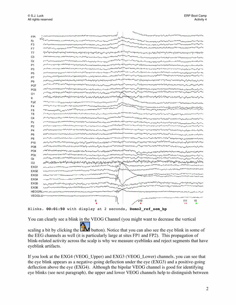
the Set Interval or Reset Interval buttons and indicating the length of time that you would like to see in the window. Now lets take a look at some artifacts. Select demo2 > RawData > Demo2_Raw > Demo2_ref_sem > Demo2_ref_sem_bp. We will use the data in Demo2 for artifact identification. Blinks Eye blinks are one of the most common artifacts in EEG data. To see an example of an eye blink, scroll to the 00:01:50 time point in the data file (with a display interval of 2 seconds), so that the center marker is between event codes 6 and 219. It should look like this:
© S.J. Luck ERP Boot Camp All rights reserved Activity 4
2
FP1FzF3F7T7C3CzP1P3P5P7P9PO7PO3O1IzFp2F4F8T8C4PzP2P4P6P8P10PO8PO4POzOzO2EXG1EXG2EXG3EXG4EXG5EXG6HEOGR-LVEOGL-U
6 219 511
50 µV
515
Blinks. 00:01:50 with display at 2 seconds, Demo2_ref_sem_bp You can clearly see a blink in the VEOG Channel (you might want to decrease the vertical
scaling a bit by clicking the button). Notice that you can also see the eye blink in some of the EEG channels as well (it is particularly large at sites FP1 and FP2). This propagation of blink-related activity across the scalp is why we measure eyeblinks and reject segments that have eyeblink artifacts. If you look at the EXG4 (VEOG_Upper) and EXG3 (VEOG_Lower) channels, you can see that the eye blink appears as a negative-going deflection under the eye (EXG3) and a positive-going deflection above the eye (EXG4). Although the bipolar VEOG channel is good for identifying eye blinks (see next paragraph), the upper and lower VEOG channels help to distinguish between

© S.J. Luck ERP Boot Camp All rights reserved Activity 4
3
eye related activity and ERPs in the averaged waveforms. Once you average the segments of data, cortically generated ERPs should be visible in the VEOG_Upper and VEOG_Lower channels, because ERPs are visible over the entire surface of the head. If you see an experimental effect in your average data that goes in opposite directions under vs. over the eyes, it is very likely that you are merely seeing differences in blinking between conditions and not a real ERP effect. We have taken advantage of the opposite polarity above and below the eye by creating a channel called VEOGL-U, in which the VEOG_Upper signal is subtracted from the VEOG_Lower signal. This is exactly what you would get by recording a bipolar signal between the VEOG_Lower site and the VEOG_Upper site (with VEOG_Upper as the reference). Because the blink signal is opposite in polarity at these two sites, subtracting the two signals leads to an increase in the size of the blink without increasing non-blink activity. This makes it easier to reject trials with blinks without also rejecting trials with non-blink activity. However, it is also useful to retain the original VEOG_Lower and VEOG_Upper signals so that we can assess polarity inversions in the averaged waveforms, as described in the previous paragraph. Horizontal Eye Movements Another common artifact in EEG data arises from horizontal eye movements, although these artifacts are subtler and harder to detect than eye blinks (unless the eye movements are very large). Whenever stimuli are presented away from the center of the screen, subjects are likely to make eye movements toward the stimuli. A horizontal eye movement can be seen in the data file at 00:03:19. However, this is a very large horizontal eye movement, and in most cases the eye movements will be much smaller and harder to distinguish (we will look at some examples of typical horizontal eye movements later). The eye movement should look like this:
© S.J. Luck ERP Boot Camp All rights reserved Activity 4
4
FP1FzF3F7T7C3CzP1P3P5P7P9PO7PO3O1IzFp2F4F8T8C4PzP2P4P6P8P10PO8PO4POzOzO2EXG1EXG2EXG3EXG4EXG5EXG6HEOGR-LVEOGL-U
228 6
50 µV
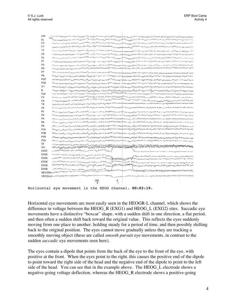
Horizontal eye movement in the HEOG channel. 00:03:19. Horizontal eye movements are most easily seen in the HEOGR-L channel, which shows the difference in voltage between the HEOG_R (EXG1) and HEOG_L (EXG2) sites. Saccadic eye movements have a distinctive “boxcar” shape, with a sudden shift in one direction, a flat period, and then often a sudden shift back toward the original value. This reflects the eyes suddenly moving from one place to another, holding steady for a period of time, and then possibly shifting back to the original position. The eyes cannot move gradually unless they are tracking a smoothly moving object (these are called smooth pursuit eye movements, in contrast to the sudden saccadic eye movements seen here). The eyes contain a dipole that points from the back of the eye to the front of the eye, with positive at the front. When the eyes point to the right, this causes the positive end of the dipole to point toward the right side of the head and the negative end of the dipole to point to the left side of the head. You can see that in the example above. The HEOG_L electrode shows a negative-going voltage deflection, whereas the HEOG_R electrode shows a positive-going
© S.J. Luck ERP Boot Camp All rights reserved Activity 4
5
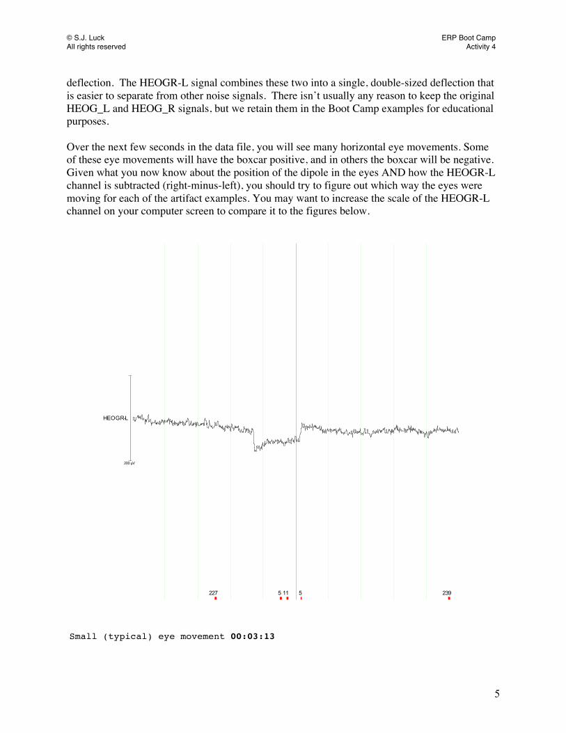
deflection. The HEOGR-L signal combines these two into a single, double-sized deflection that is easier to separate from other noise signals. There isn’t usually any reason to keep the original HEOG_L and HEOG_R signals, but we retain them in the Boot Camp examples for educational purposes. Over the next few seconds in the data file, you will see many horizontal eye movements. Some of these eye movements will have the boxcar positive, and in others the boxcar will be negative. Given what you now know about the position of the dipole in the eyes AND how the HEOGR-L channel is subtracted (right-minus-left), you should try to figure out which way the eyes were moving for each of the artifact examples. You may want to increase the scale of the HEOGR-L channel on your computer screen to compare it to the figures below.
HEOGR-L
227 5 11 5 239
200 µV
Small (typical) eye movement 00:03:13

© S.J. Luck ERP Boot Camp All rights reserved Activity 4
6
HEOGR-L
500 µV
247 11 155
Large (atypical) eye movement preceded by a small eye movement 00:03:16. Try to scan throughout other sections of the dataset to find small horizontal eye movements. Note that there is often a small, sharp voltage spike at the beginning of an eye movement; this is EMG activity from the extraocular muscles that cause the eyes to rotate. These muscles contract briefly to rotate the eyes, but they do not continue to contract once the eyes have moved (the eyes stay in the new position without any significant muscle activity). Skin Potentials Skin potentials are another common artifact. Skin potentials are caused by small voltage changes at an electrode site and are commonly caused by the subject sweating (often imperceptibly). There are sweat glands located all over the head, so it is very important to try to minimize sweating by keeping the recording chamber cool and dry. If you change the scale of the window from 2 seconds to 10 seconds you can see voltage changes that are happening over longer periods of time. If you look at time point 00:06:12 you will see drifting in electrodes Fp1, Fp2, PO7, as well as some eye channels. This drifting is most likely caused by skin potentials.

© S.J. Luck ERP Boot Camp All rights reserved Activity 4
7
C.R.A.P. Another artifact we commonly see in EEG data is what we call C.R.A.P. (or Commonly Recorded Artifactual Potentials). These are miscellaneous artifacts, usually of unknown origin. You can see an example in channel O2 during the time frame in which the skin potentials are happening. If you saw an artifact like this during data collection, you would want to pause the experiment and fix the electrode. Scroll to time point 00:06:26. Notice the oscillations in channel F8. If you change the display interval to 100 ms (.1 s), you can see that there are 6 peaks in 100 ms, which is equal to 60 peaks in 1000 ms (or 60 Hz). Thus, for some reason, 60 Hz noise was being picked up by the F8 electrode at that time. Muscle Activity Muscle activity (EMG) is another artifact that you often see. It is very fast activity that has both positive and negative spikes. Scroll to time point 00:05:51. Change the interval back to two seconds and start scrolling through the data. You will notice that a good portion of the channels are very clean; however, there is quite a bit of muscle activity in the eye channels and FP1 and FP2. Muscle activity consists of fairly irregular high-frequency noise (little spikes of varying sizes). Before you read on, think of a reason why you might see muscle activity in these particular channels – are there muscles nearby? When participants are concentrating or are tired and trying to stay awake, you may notice a lot of activity in FP1 and FP2. This is because they are lifting their eyebrows or scrunching up the forehead in an attempt to focus. By making the participants aware of this activity and telling them to relax the forehead, you can usually reduce these artifacts. Scroll to time point 00:08:09. Take a close look at this muscle activity. You may notice that a lot of the muscle activity takes place at T7/T8 and F7/F8, as well as some of the eye areas. This muscle activity is due to jaw clenching. The very powerful jaw muscles are close to these electrodes, and when a subject is tense, this can cause C.R.A.P.py data. The T7/T8 sites usually exhibit some visible EMG activity, even if the subject tries very hard to relax the jaw muscles. Scroll through the next few minutes of data and you will see lot of muscle activity, concentrated around the eyes. In this case, the muscle activity is caused by smiling (not a common problem in actual experiments!).

© S.J. Luck ERP Boot Camp All rights reserved Activity 4
8
FP1FzF3F7T7C3CzP1P3P5P7P9PO7PO3O1IzFp2F4F8T8C4PzP2P4P6P8P10PO8PO4POzOzO2EXG1EXG2EXG3EXG4EXG5EXG6HEOGR-LVEOGL-U
50 µV
246 6 227
00:10:40 Time Range : 00:10:32-00:10:53 Notice that the channels in this time segment are simply noisier than in previous segments. The participant is probably getting antsy, tired, and is tensing up some muscles. This is probably a good time to take a break and have the participant relax or stretch. To avoid this sort of noise, it is generally a good idea to have brief breaks throughout the experiment and not to have the subject in the chamber for more than 1.5–2 hours, provided your experimental design can operate under those constraints.
© S.J. Luck ERP Boot Camp All rights reserved Activity 4
9
Fp1FzF3F7T7C3CzP1P3P5P7P9PO7PO3O1IzFp2F4F8T8C4PzP2P4P6P8P10PO8PO4POzOzO2EXG1EXG2EXG3EXG4EXG5EXG6Status
5 249 511 5
50 µV
15611
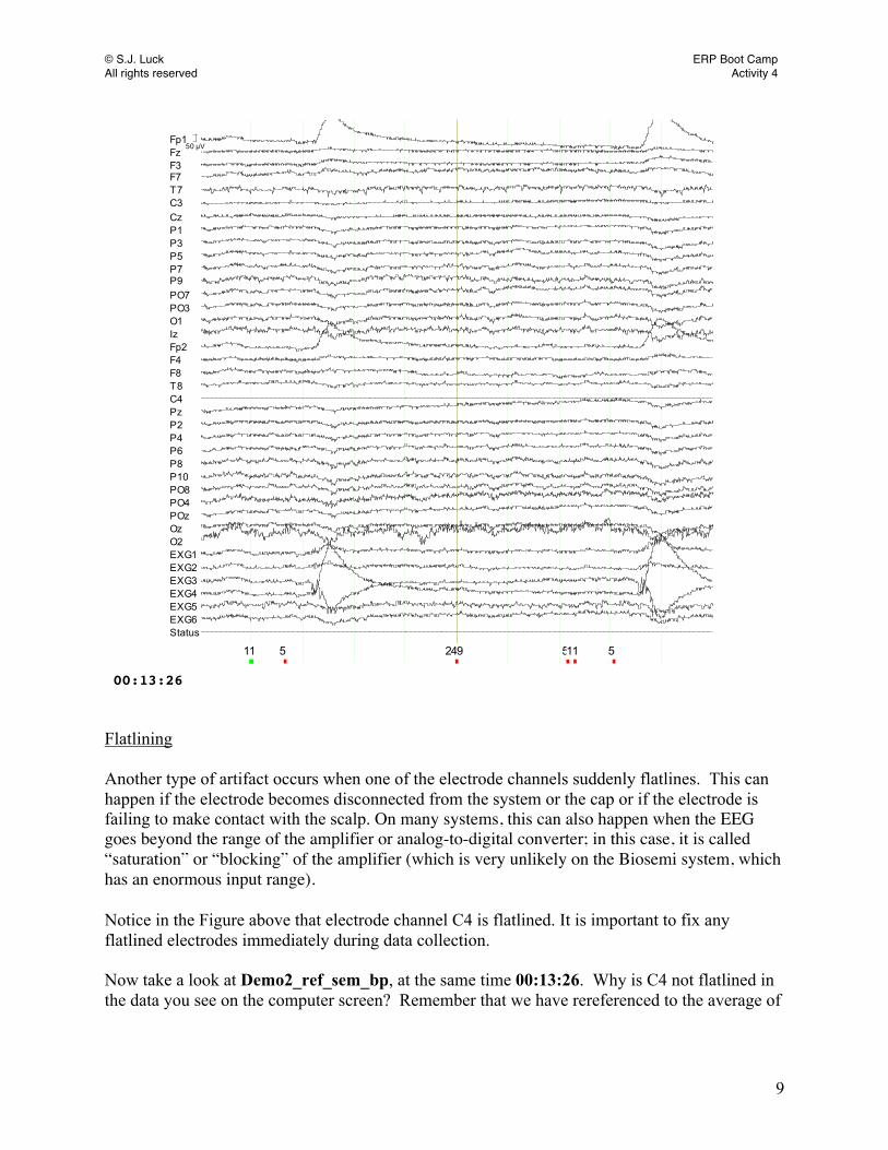
00:13:26 Flatlining Another type of artifact occurs when one of the electrode channels suddenly flatlines. This can happen if the electrode becomes disconnected from the system or the cap or if the electrode is failing to make contact with the scalp. On many systems, this can also happen when the EEG goes beyond the range of the amplifier or analog-to-digital converter; in this case, it is called “saturation” or “blocking” of the amplifier (which is very unlikely on the Biosemi system, which has an enormous input range). Notice in the Figure above that electrode channel C4 is flatlined. It is important to fix any flatlined electrodes immediately during data collection. Now take a look at Demo2_ref_sem_bp, at the same time 00:13:26. Why is C4 not flatlined in the data you see on the computer screen? Remember that we have rereferenced to the average of
© S.J. Luck ERP Boot Camp All rights reserved Activity 4
10
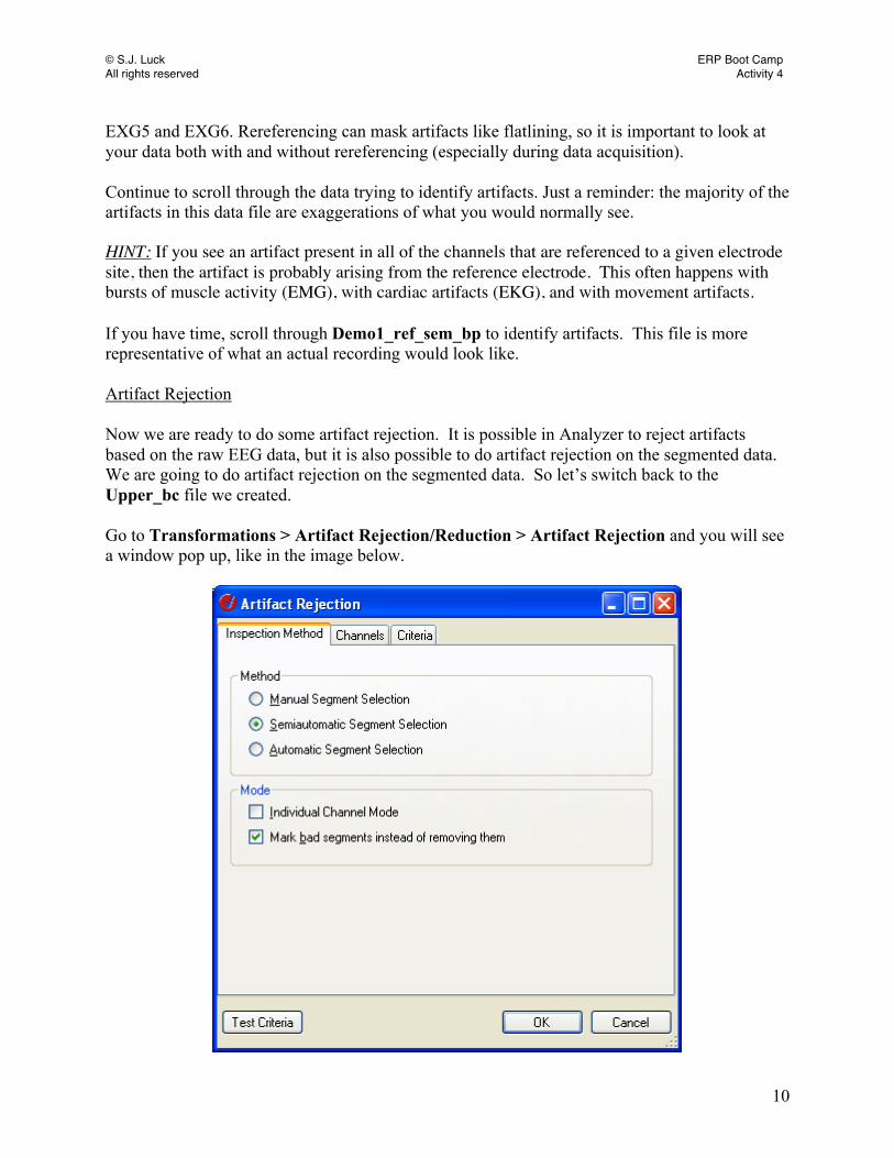
EXG5 and EXG6. Rereferencing can mask artifacts like flatlining, so it is important to look at your data both with and without rereferencing (especially during data acquisition). Continue to scroll through the data trying to identify artifacts. Just a reminder: the majority of the artifacts in this data file are exaggerations of what you would normally see. HINT: If you see an artifact present in all of the channels that are referenced to a given electrode site, then the artifact is probably arising from the reference electrode. This often happens with bursts of muscle activity (EMG), with cardiac artifacts (EKG), and with movement artifacts. If you have time, scroll through Demo1_ref_sem_bp to identify artifacts. This file is more representative of what an actual recording would look like. Artifact Rejection Now we are ready to do some artifact rejection. It is possible in Analyzer to reject artifacts based on the raw EEG data, but it is also possible to do artifact rejection on the segmented data. We are going to do artifact rejection on the segmented data. So let’s switch back to the Upper_bc file we created. Go to Transformations > Artifact Rejection/Reduction > Artifact Rejection and you will see a window pop up, like in the image below.

© S.J. Luck ERP Boot Camp All rights reserved Activity 4
11
There are three options for performing artifact rejection: Manual Segment Selection: This selection allows you to go through the data manually and select the segments to keep or reject on the basis of visual inspection. However, this requires you to examine every segment of data, and it is a tedious process that might end up biasing your results. Semiautomatic Segment Selection: You select the channels and criteria for artifact rejection and then have the option of manually accepting or rejecting segments to assess how well artifact rejection was performed. You set thresholds for Gradient, Max-Min, Amplitude, and Low Activity (explained in detail below). Based on these thresholds the program will either Keep or Reject each segment. You then have the option to go through the data like in manual segment selection to see if your criteria reject the appropriate segments. That way if the artifact rejection seems too strict (meaning you are rejecting segments with clean data) or is failing to capture the majority of the artifacts in the data, you can adjust your criteria and rerun the artifact rejection. However, it is important to make sure that you cannot somehow bias your results by using different rejection criteria for different conditions or subject groups. Automatic Segment Selection: This is the same as Semiautomatic Segment Selection, except that it does not allow you to scroll through the segments or to go back and adjust the criteria. We will be using Semiautomatic Segment Selection so that we can see how the selected criteria interact with the data as well as change the criteria if necessary. This is usually recommended, because some artifacts will appear in some subjects but not others and artifacts can drastically vary in size from subject to subject. There are two other options when running artifact rejection: Individual Channel Mode: Instead of rejecting an entire segment, this option simply removes the particular channel(s) with the artifact and leaves the remaining channels as accepted segments. Leave this box unchecked and think about why this option is a bad idea. HINT: remember how artifacts in LM and RM affected the rest of the electrodes on the scalp AND how blinks would appear in FP1 and FP2. However, this option is useful if one particular channel was bad throughout the experiment and needs to be removed. Mark bad segments instead of removing them: Check this box! This allows you to see how well your artifact rejection criteria are doing at getting rid of artifacts. Next, click on the Channels tab at the top of the window. You should see the following:
© S.J. Luck ERP Boot Camp All rights reserved Activity 4
12
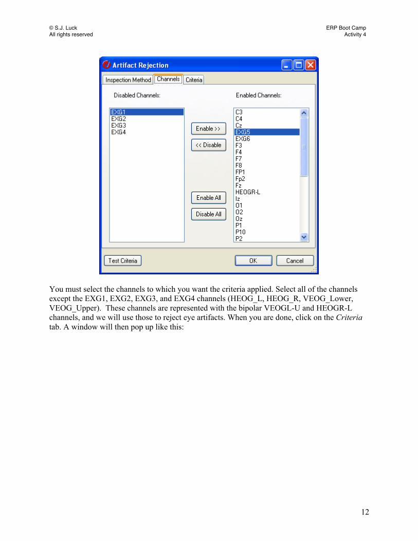
You must select the channels to which you want the criteria applied. Select all of the channels except the EXG1, EXG2, EXG3, and EXG4 channels (HEOG_L, HEOG_R, VEOG_Lower, VEOG_Upper). These channels are represented with the bipolar VEOGL-U and HEOGR-L channels, and we will use those to reject eye artifacts. When you are done, click on the Criteria tab. A window will then pop up like this:
© S.J. Luck ERP Boot Camp All rights reserved Activity 4
13
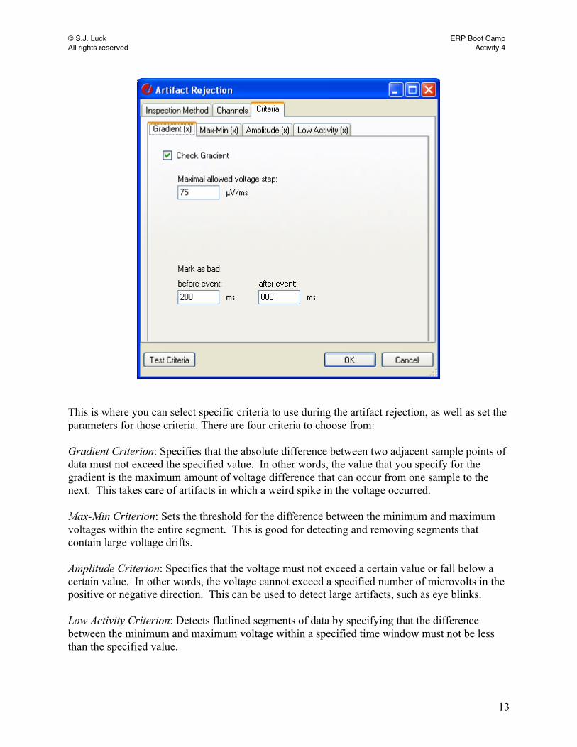
This is where you can select specific criteria to use during the artifact rejection, as well as set the parameters for those criteria. There are four criteria to choose from: Gradient Criterion: Specifies that the absolute difference between two adjacent sample points of data must not exceed the specified value. In other words, the value that you specify for the gradient is the maximum amount of voltage difference that can occur from one sample to the next. This takes care of artifacts in which a weird spike in the voltage occurred. Max-Min Criterion: Sets the threshold for the difference between the minimum and maximum voltages within the entire segment. This is good for detecting and removing segments that contain large voltage drifts. Amplitude Criterion: Specifies that the voltage must not exceed a certain value or fall below a certain value. In other words, the voltage cannot exceed a specified number of microvolts in the positive or negative direction. This can be used to detect large artifacts, such as eye blinks. Low Activity Criterion: Detects flatlined segments of data by specifying that the difference between the minimum and maximum voltage within a specified time window must not be less than the specified value.
© S.J. Luck ERP Boot Camp All rights reserved Activity 4
14
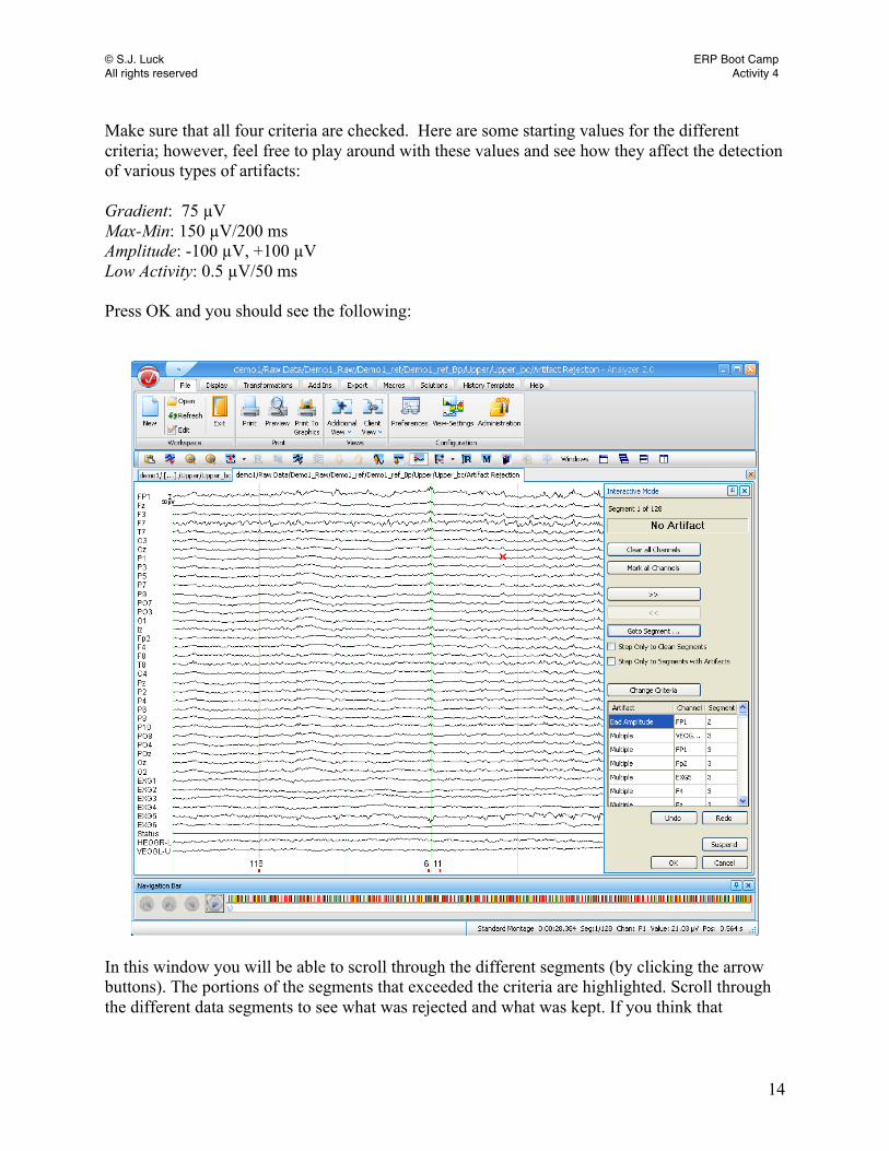
Make sure that all four criteria are checked. Here are some starting values for the different criteria; however, feel free to play around with these values and see how they affect the detection of various types of artifacts: Gradient: 75 µV Max-Min: 150 µV/200 ms Amplitude: -100 µV, +100 µV Low Activity: 0.5 µV/50 ms Press OK and you should see the following:
In this window you will be able to scroll through the different segments (by clicking the arrow buttons). The portions of the segments that exceeded the criteria are highlighted. Scroll through the different data segments to see what was rejected and what was kept. If you think that
© S.J. Luck ERP Boot Camp All rights reserved Activity 4
15
something was rejected and it should have been kept, you may need to go back and change the criteria. You can easily do this by pressing the Change Criteria button. You may also want to do two stages of artifact rejection: one stage for general artifact rejection and a second stage to apply artifact rejection with a stricter criterion on only the VEOG and/or HEOG channels. This is sometimes helpful to make sure you get rid of all of the eye movements and blinks. Click OK, and a new node with all of the segments that were not rejected will be created. Remember to rename the node Upper_arf. How can you tell if you’ve done an adequate job of artifact rejection? As described in the ERP book, artifact detection is essentially a signal detection problem with hits (rejection of trials with actual artifacts), misses (failure to reject trials with actual artifacts), correction rejections (acceptance of trials without actual artifacts), and false alarms (rejection of trials without actual artifacts). You should be able to distinguish between these possibilities for each segment by visually inspecting the data when the artifacts are large (like blinks and large eye movements, especially when the EEG is otherwise clean). However, it can be hard to know whether you’ve done a good job of rejecting artifacts that are small compared to the noise level (such as small eye movements). Moreover, when the data contain large numbers of relatively slow voltage deflections, it may be difficult to reject all blinks without also rejecting some segments that have slow voltage shifts. You may end up rejecting so many segments that the signal-to-noise ratio is actually worse as a result of artifact rejection. It is a good idea to check after performing artifact rejection to see how many segments were rejected and how many remaining segments you have before averaging the data. In many cases, you can assess the adequacy of your artifact rejection procedures by looking at the averaged ERP waveforms, in which the noise level is considerably smaller than that of the raw EEG. The next section will explain how to average the data to assess the quality of the artifact rejection. Now perform artifact rejection on the lower segments and the LRP segments. You can do this by dragging the Upper_arf node onto the node you wish to artifact reject. You will then need to go through the segments to make sure that the rejection is working properly, and then click OK. Remember to rename the new nodes. Averaging to Assess Artifact Rejection Adequacy A good way to tell if artifact rejection was successful to is to look at the averaged waveforms. If the averaged waveforms look clean and the VEOG and HEOG channels show no sign of artifacts, then you probably were successful at artifact rejection. However, if there are significant artifacts that remain in the averaged waveforms, you should try cleaning up the data by redoing the artifact rejection. Averaging using Analyzer is very easy. Double click on the artifact rejected segmented node (e.g., Upper_arf) and go to Transformations > Segment Analysis Functions > Average. A box like the one below will appear prompting you for the parameters for averaging the segments. For this exercise we only want Use Full Range selected. The rest of the options allow you to

© S.J. Luck ERP Boot Camp All rights reserved Activity 4
16
average only some of the segments. For example, you could average together the first half or only the odd segments.
Click OK and this will create an average for the segments in the selected file. Look at the VEOGL-U channel (if you double click on the name, the VEOGL-U window will be maximized). In order to have a baseline for the plotted waveforms, right click in the window, select Grid View Settings, the Display tab, and check the box for Show Baseline. The VEOGL-U channel should be relatively flat and have no distinct artifacts (it will not be perfectly flat, because any ERP activity that differs between the sites above and below the eyes will be picked up by these electrodes, but such activity is usually quite small). If there is a large potential in the VEOG channel, your criteria were probably not strict enough. This means you should go back to artifact rejection and change the values to make them stricter or perform a second artifact rejection using only the eye channels. There are two things that you should always look for in the averaged VEOG. First, is there a deflection at the beginning of the waveform that falls off over time? If so, then the subject probably tended to blink 500-1000 ms before the stimulus. The voltage was not large enough by the time of the stimulus for the trial to be rejected, but it might still be relatively large in the average if it occurred on a significant proportion of trials. You can sometimes solve this by using a longer prestimulus interval for artifact rejection. Second, is your VEOG waveform opposite in polarity to the waveforms at the frontal electrode sites? (Or opposite in polarity to the experimental effect at the frontal sites?) When the VEOG signal is computed as VEOG-Lower minus VEOG-Upper, any actual eyeblink activity should be opposite in polarity in the VEOG signal compared to the frontal sites. Thus, the absence of an opposite-polarity signal at these sites means that you probably do not have any significant eyeblink confounds and the activity is ERP activity.

© S.J. Luck ERP Boot Camp All rights reserved Activity 4
17
Once you have no artifacts in the eye channels (or any of the other channels), artifact rejection is complete. Remember to rename the averaged file Avg_Upper. Make averages for the lower segments and the LRP segments to check your artifact rejection there. You can do this by dragging the Avg_Upper node onto the segmented nodes you wish to average. Remember to rename the new nodes.
© S.J. Luck ERP Boot Camp All rights reserved Activity 5
1
Activity 5 Linear Recombinations: Creating Difference Waves
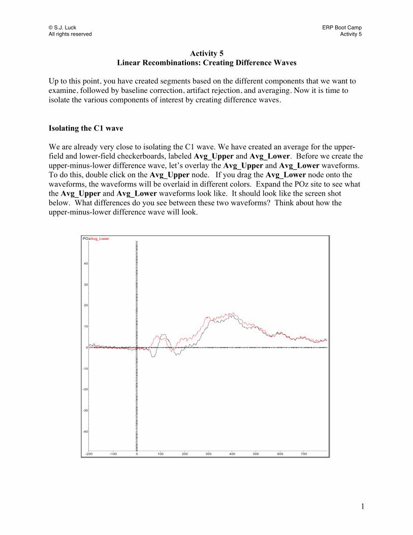
Up to this point, you have created segments based on the different components that we want to examine, followed by baseline correction, artifact rejection, and averaging. Now it is time to isolate the various components of interest by creating difference waves. Isolating the C1 wave We are already very close to isolating the C1 wave. We have created an average for the upper-field and lower-field checkerboards, labeled Avg_Upper and Avg_Lower. Before we create the upper-minus-lower difference wave, let’s overlay the Avg_Upper and Avg_Lower waveforms. To do this, double click on the Avg_Upper node. If you drag the Avg_Lower node onto the waveforms, the waveforms will be overlaid in different colors. Expand the POz site to see what the Avg_Upper and Avg_Lower waveforms look like. It should look like the screen shot below. What differences do you see between these two waveforms? Think about how the upper-minus-lower difference wave will look.
POzAvg_Lower
-200 -100 0 100 200 300 400 500 600 700
-40
-30
-20
-10
0
10
20
30
40

© S.J. Luck ERP Boot Camp All rights reserved Activity 5
2
Now all we need to do is create an upper-minus-lower difference wave. Double click on Avg_Upper then select Transformations > Comparisons and Statistics > Data Comparison. Under Comparison Methods, select Difference and then press OK. A new window will pop up. Under Data Sources select Compare Datasets and then press Next. A new window will pop up. If you click on Expand All, the nodes under the trees for each of the demos will appear. Select Avg_Lower under the Demo1 tree as the dataset that you would like to compare. When you have selected the desired node press Finish. A new node will be created under Avg_Upper labeled Diff. Waves. Rename the new file C1_Upper-Lower.
Maximize electrode POz by double clicking on the electrode name. You should now see three waveforms in the display: one red, one blue and one black. The black one is the difference wave,

© S.J. Luck ERP Boot Camp All rights reserved Activity 5
3
and the red and blue waveforms are from Avg_Upper and Avg_Lower, respectively. Take a close look at these three waveforms. Look at the difference between the parent and the other waveform. Subtracting the other from the parent is what yields the difference wave. If you want to see just the difference wave without the parent waveforms overlaid, simply click on parent and other next to the electrode channel label to remove them from the display. Now you can see what the C1 waveform looks like. It is the negative deflection at approximately 75 ms. Isolating the LRP Component Now we will walk through the isolation of the LRP component. This component (as well as the N2pc) is substantially more complicated to isolate, because it requires a contralateral-minus-ipsilateral difference wave. We will create contra-minus-ipsi difference waves for all of the electrodes, except those on the midline. All of the odd-numbered electrode sites (e.g. C3, Fp1) are contralateral when subjects make a right-hand response, but these same electrode sites are ipsilateral when subjects make a left-hand response. All of the even number electrode sites (e.g., C4, FP2) are contralateral when subjects make a left-hand response, but these same electrode sites are ipsilateral when subjects make a right-hand response. This is why the LRP, and the N2pc, are more complicated to isolate. In addition, it is important to collapse across left-hand and right-hand response trials (to avoid any effects of response hand that are not lateralized) and across the left and right hemispheres (to avoid any overall lateralizations that are unrelated to the side of the response). There are several ways that we could do this, but we will take a strategy that will (we hope!) make the logic very clear. The basic idea is to start by creating 4 separate averages: (1) left-hand response, contra electrodes; (2) left-hand response, ipsi electrodes; (3) right-hand response, contra electrodes; and (4) right-hand response, ipsi electrodes. To do this, we will use the Transformations > Data Preprocessing > Linear Derivations command to select the appropriate electrode sites for each average and give it the same name (e.g. “FP1/FP2”) in all average files (which will be necessary when we collapse across hemispheres at a later stage). As discussed in a previous tutorial, the Linear Derivations command is used to create new channels that are linear combinations of existing channels (i.e., summed and scaled combinations, such as subtracting half of the mastoids in the rereferencing process). Here, we will use Linear Derivations to do a very simple process, creating a single channel, such as “FP1/FP2” that will be either the FP1 site or the FP2 site, depending on which hand responded and whether we want the ipsi hemisphere or the contra hemisphere. Specifically, we will create four average files, each with 13 channels (FP1/FP2, F3/F4, F7/F8, C3/C4, T7/T8, P1/P2, P3/P4, P5/P6, P7/P8, P9/P10, PO3/PO4, PO7/PO8, O1/O2): (1) lhand contra (left hand response, even electrodes); (2) lhand ipsi (left hand response, odd electrodes); (3) rhand contra (right hand response, odd electrodes); and (4) rhand ipsi (right hand response, even electrodes). We will then create an average of the two ipsi waveforms (called ipsi_resp) and an average of the two contra waveforms (called contra_resp) and a difference waveform in which we subtract ipsi from contra (called LRP_contra-ipsi).

© S.J. Luck ERP Boot Camp All rights reserved Activity 5
4
Ok, now let’s break this down, step by step. Double click on the Avg_Right_Resp node. Go to Transformations > Dataset Preprocessing > Linear Derivations and load the rhand contra derivation file (under C:\Bootcamp_Analyzer2\workfiles). Before you press OK, take a look at the file. Notice how the electrodes in the left hemisphere are those that have a weighting of 1. This is because we want to select those electrode sites that are contralateral to the right hand response, i.e., the left hemisphere sites. Go ahead and press OK and rename the node rh contra. Now create the rh ipsi file using the rh ipsi derivation file. Once you have finished with that, switch over to the Avg_Left_resp, and create an lh contra node and an lh ipsi node. Once you have created these four files, you need to average together the two contra files to create a contra_resp, and then average together the two ipsi files to create an ipsi_resp file. Go to Transformations > Segment Analysis Functions > Result Evaluation > Grand Average and you will see a window like this:
Although the term grand average is usually used to refer to averages over multiple subjects, the Analyzer program uses this term whenever it averages across multiple files. You must input the nodes that you want averaged together in the left hand column of Input History Nodes & Output
© S.J. Luck ERP Boot Camp All rights reserved Activity 5
5
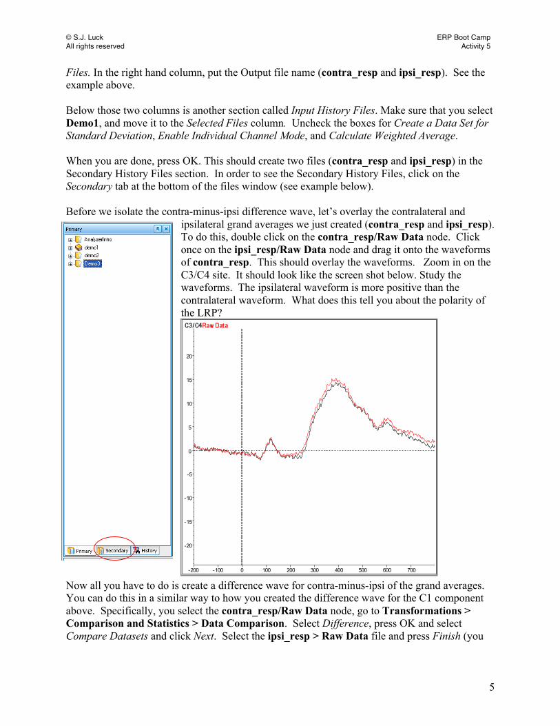
Files. In the right hand column, put the Output file name (contra_resp and ipsi_resp). See the example above. Below those two columns is another section called Input History Files. Make sure that you select Demo1, and move it to the Selected Files column. Uncheck the boxes for Create a Data Set for Standard Deviation, Enable Individual Channel Mode, and Calculate Weighted Average. When you are done, press OK. This should create two files (contra_resp and ipsi_resp) in the Secondary History Files section. In order to see the Secondary History Files, click on the Secondary tab at the bottom of the files window (see example below). Before we isolate the contra-minus-ipsi difference wave, let’s overlay the contralateral and
ipsilateral grand averages we just created (contra_resp and ipsi_resp). To do this, double click on the contra_resp/Raw Data node. Click once on the ipsi_resp/Raw Data node and drag it onto the waveforms of contra_resp. This should overlay the waveforms. Zoom in on the C3/C4 site. It should look like the screen shot below. Study the waveforms. The ipsilateral waveform is more positive than the contralateral waveform. What does this tell you about the polarity of the LRP?
Now all you have to do is create a difference wave for contra-minus-ipsi of the grand averages. You can do this in a similar way to how you created the difference wave for the C1 component above. Specifically, you select the contra_resp/Raw Data node, go to Transformations > Comparison and Statistics > Data Comparison. Select Difference, press OK and select Compare Datasets and click Next. Select the ipsi_resp > Raw Data file and press Finish (you

© S.J. Luck ERP Boot Camp All rights reserved Activity 5
6
may have to select Expand All to make it visible). This will perform the contra minus ipsi subtraction. Rename the difference wave node LRP_contra-ipsi. The file should look like this at electrode C3/4:
The LRP is relatively small, so you may have to change the vertical scaling in order to see the component. The black line represents the difference wave and the red and blue waveforms (which may appear superimposed on the difference wave on your computer screen) are the parent waveforms from which the difference wave was created. The LRP starts around 200 ms and is the negative voltage deflection that persists thereafter. Remember, if you want to see just the difference wave without the parent waveforms overlaid simply click on the parent and other labels next to the electrode channel label.
© S.J. Luck ERP Boot Camp All rights reserved Activity 6
1
Activity 6 Measuring ERP Components
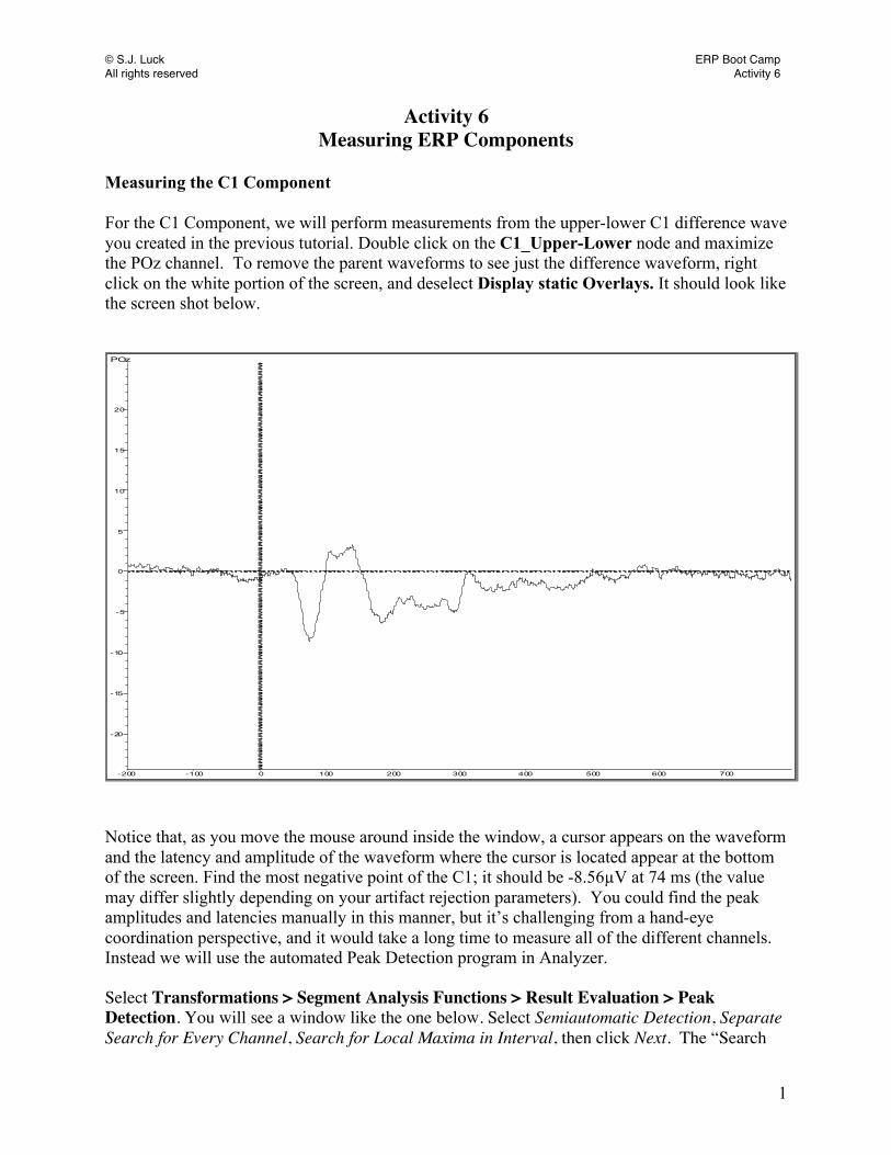
Measuring the C1 Component For the C1 Component, we will perform measurements from the upper-lower C1 difference wave you created in the previous tutorial. Double click on the C1_Upper-Lower node and maximize the POz channel. To remove the parent waveforms to see just the difference waveform, right click on the white portion of the screen, and deselect Display static Overlays. It should look like the screen shot below. POz
-200 -100 0 100 200 300 400 500 600 700
-20
-15
-10
-5
0
5
10
15
20
Notice that, as you move the mouse around inside the window, a cursor appears on the waveform and the latency and amplitude of the waveform where the cursor is located appear at the bottom of the screen. Find the most negative point of the C1; it should be -8.56µV at 74 ms (the value may differ slightly depending on your artifact rejection parameters). You could find the peak amplitudes and latencies manually in this manner, but it’s challenging from a hand-eye coordination perspective, and it would take a long time to measure all of the different channels. Instead we will use the automated Peak Detection program in Analyzer. Select Transformations > Segment Analysis Functions > Result Evaluation > Peak Detection. You will see a window like the one below. Select Semiautomatic Detection, Separate Search for Every Channel, Search for Local Maxima in Interval, then click Next. The “Search

© S.J. Luck ERP Boot Camp All rights reserved Activity 6
2
for Local Maxima in Interval” option tells it to find a local peak (e.g., a point surrounded by smaller points on each side), which is the method recommended in the ERP book. Local peak detection ensures that you do not find the rising or falling edge of a preceding or following component instead of the peak of the component of interest.
A new box will appear, like this:
© S.J. Luck ERP Boot Camp All rights reserved Activity 6
3
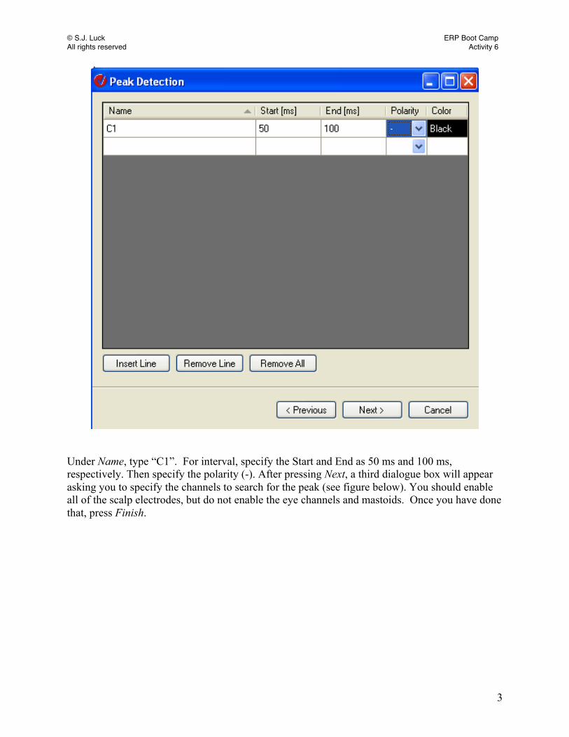
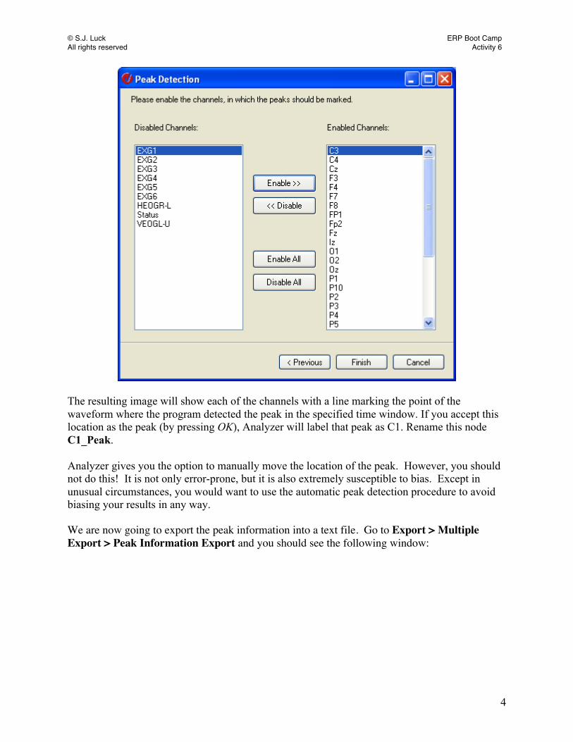
Under Name, type “C1”. For interval, specify the Start and End as 50 ms and 100 ms, respectively. Then specify the polarity (-). After pressing Next, a third dialogue box will appear asking you to specify the channels to search for the peak (see figure below). You should enable all of the scalp electrodes, but do not enable the eye channels and mastoids. Once you have done that, press Finish.
© S.J. Luck ERP Boot Camp All rights reserved Activity 6
4
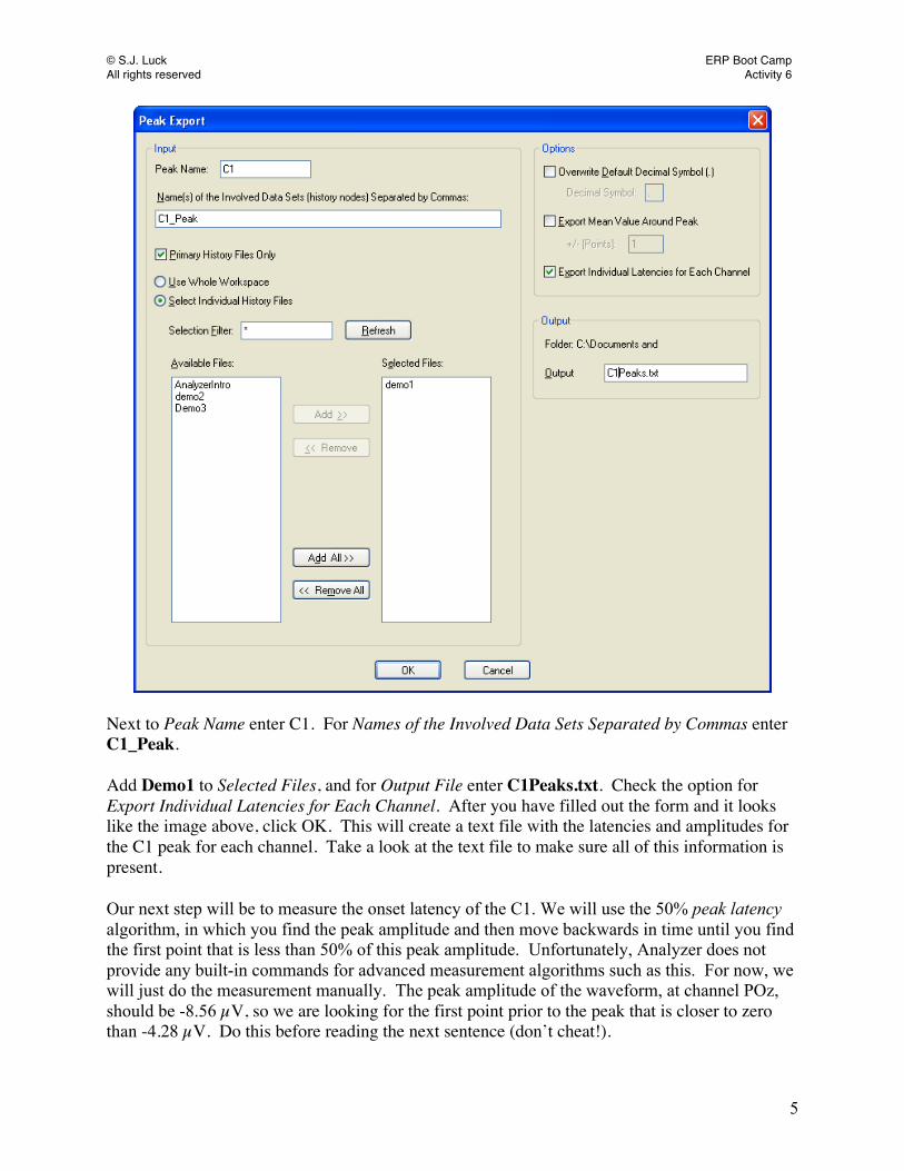
The resulting image will show each of the channels with a line marking the point of the waveform where the program detected the peak in the specified time window. If you accept this location as the peak (by pressing OK), Analyzer will label that peak as C1. Rename this node C1_Peak. Analyzer gives you the option to manually move the location of the peak. However, you should not do this! It is not only error-prone, but it is also extremely susceptible to bias. Except in unusual circumstances, you would want to use the automatic peak detection procedure to avoid biasing your results in any way. We are now going to export the peak information into a text file. Go to Export > Multiple Export > Peak Information Export and you should see the following window:
© S.J. Luck ERP Boot Camp All rights reserved Activity 6
5
Next to Peak Name enter C1. For Names of the Involved Data Sets Separated by Commas enter C1_Peak. Add Demo1 to Selected Files, and for Output File enter C1Peaks.txt. Check the option for Export Individual Latencies for Each Channel. After you have filled out the form and it looks like the image above, click OK. This will create a text file with the latencies and amplitudes for the C1 peak for each channel. Take a look at the text file to make sure all of this information is present. Our next step will be to measure the onset latency of the C1. We will use the 50% peak latency algorithm, in which you find the peak amplitude and then move backwards in time until you find the first point that is less than 50% of this peak amplitude. Unfortunately, Analyzer does not provide any built-in commands for advanced measurement algorithms such as this. For now, we will just do the measurement manually. The peak amplitude of the waveform, at channel POz, should be -8.56 µV, so we are looking for the first point prior to the peak that is closer to zero than -4.28 µV. Do this before reading the next sentence (don’t cheat!).
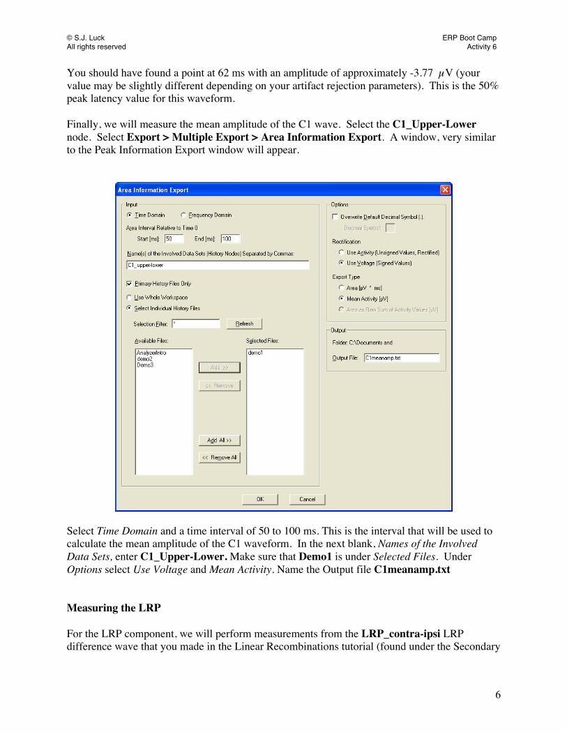
© S.J. Luck ERP Boot Camp All rights reserved Activity 6
6
You should have found a point at 62 ms with an amplitude of approximately -3.77 µV (your value may be slightly different depending on your artifact rejection parameters). This is the 50% peak latency value for this waveform. Finally, we will measure the mean amplitude of the C1 wave. Select the C1_Upper-Lower node. Select Export > Multiple Export > Area Information Export. A window, very similar to the Peak Information Export window will appear.
Select Time Domain and a time interval of 50 to 100 ms. This is the interval that will be used to calculate the mean amplitude of the C1 waveform. In the next blank, Names of the Involved Data Sets, enter C1_Upper-Lower. Make sure that Demo1 is under Selected Files. Under Options select Use Voltage and Mean Activity. Name the Output file C1meanamp.txt Measuring the LRP For the LRP component, we will perform measurements from the LRP_contra-ipsi LRP difference wave that you made in the Linear Recombinations tutorial (found under the Secondary

© S.J. Luck ERP Boot Camp All rights reserved Activity 6
7
file tab). For peak amplitude and latency, use a search interval of 200 to 450ms. For mean amplitude, use a range of 250 to 400 ms. Export this information. For peak measures, it is generally a good idea to filter your data with a low-pass filter before performing the measurements. Think about why this might be the case. Peak measures, such as peak latency and peak amplitude, find the most extreme voltage in a particular window. If there is a lot of high frequency noise, a peak associated with that noise may be the most negative or positive point, and the peak detection program may mark that point as the component. Let’s filter the LRP waveform with a low-pass filter and re-measure the peak latency and peak amplitude. Select Transformations > Artifact Rejection/Reduction > Data Filtering > IIR Filters and specify a low-pass filter (high cutoff) of 30 Hz with a roll-off of 12 dB/octave. The waveform should now look like the figure below. Note that the amplitude at this point is now smaller (less negative) than it was in the unfiltered data. Export the values for both the filtered and unfiltered peaks and compare the values.

© S.J. Luck ERP Boot Camp All rights reserved Activity 6
8
Now find the 50% latency point (in the filtered waveform) and compute the mean amplitude (on the unfiltered waveform). As discussed in the boot camp lecture, filtering does not help with measuring the mean amplitude of a waveform, because mean amplitude measures are not affected by high frequency noise.

© S.J. Luck ERP Boot Camp All rights reserved Activity 7
1
Activity 7 The P3 and N2pc Components
Now that we have gone through the analysis of the C1 and LRP components, you are ready to isolate the P3 and N2pc components. Segmentation In order to isolate the P3, we want to create two different segmentations—one corresponding to rare stimuli, and one corresponding to frequent stimuli. Recall that in the MONSTER paradigm, both the A and B stimuli were rare (20% probable) and frequent (80% probable) at some point during the experiment. Therefore, we will make one segmentation node for the Rare stimuli (averaged across the As and Bs when each was 20% probable) and a second segmentation node for the Frequent stimuli (averaged across As and Bs when each was 80% probable). Go ahead and figure out which event codes should be in the Rare and Frequent segments. After double checking with the event codes file, go ahead and create the segments. Remember to rename the nodes. For the N2pc, you need to create segments for targets located in the left visual field (Targets_left_side), and segments for targets located in the right visual field (Targets_right_side). Figure out the event codes to include in the segments and then create the segments (note: these will be the codes for left side targets and right side targets in the event codes file). Baseline Correction, Artifact Rejection, Averaging Just like the C1 and LRP components, after we have created segments for the P3 and N2pc, we need to baseline correct the data, do artifact rejection, and then create averages of the segments. Linear Recombinations: Constructing Difference Waves The P3 analysis is very similar to the analysis we did for the C1 wave. We are interested in the difference between rare and frequent stimuli, so we want to make a difference wave of the rare-minus-frequent P3. First overlay the Rare and Frequent waveforms so that you can see how the difference wave isolates the difference between these two waveforms. Then isolate the rare-minus-frequent difference wave. It should look like the figure below at electrode site Pz (parent waveforms overlaid).
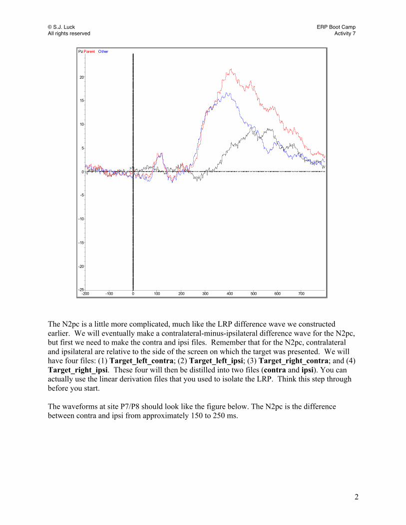
© S.J. Luck ERP Boot Camp All rights reserved Activity 7
2
PzParent Other
-200 -100 0 100 200 300 400 500 600 700-25
-20
-15
-10
-5
0
5
10
15
20
The N2pc is a little more complicated, much like the LRP difference wave we constructed earlier. We will eventually make a contralateral-minus-ipsilateral difference wave for the N2pc, but first we need to make the contra and ipsi files. Remember that for the N2pc, contralateral and ipsilateral are relative to the side of the screen on which the target was presented. We will have four files: (1) Target_left_contra; (2) Target_left_ipsi; (3) Target_right_contra; and (4) Target_right_ipsi. These four will then be distilled into two files (contra and ipsi). You can actually use the linear derivation files that you used to isolate the LRP. Think this step through before you start. The waveforms at site P7/P8 should look like the figure below. The N2pc is the difference between contra and ipsi from approximately 150 to 250 ms.

© S.J. Luck ERP Boot Camp All rights reserved Activity 7
3
P7/P8Parent Other
-200 -100 0 100 200 300 400 500 600 700
-10
-5
0
5
10
Measuring Once you have isolated the P3 in the Rare-Freq file, you can start measuring the P3. Use electrode channel Pz to do most of your measurements. For the peak amplitude, use a window of 200 to 600 ms. Find the 50% peak latency. Find the mean amplitude using a window of 300 to 600 ms. For the N2pc, use electrode channel P7/P8 to find the most negative peak between 150 and 250 ms. For your mean amplitude measurement, use a window of 150 to 250 ms. Additional Analyses Once you have completed the basic analysis steps for the P3 and N2pc, return to the N2pc analysis. One cool thing about the way the N2pc is isolated is that if you look at the HEOG channels, you can tell if subjects were making eye movements in the direction of the target stimuli. Let’s think through the logic of this. Remember that the dipole in the eye is positive in the front and negative in the back. For rightward eye movements, the voltage of the HEOG_R channel should be positive, and the voltage of the HEOG_L channel should be negative. Therefore, the voltage of the HEOGR-L channel (which is HEOG_R minus HEOG_L) should be positive for rightward eye movements. For leftward eye movements, the voltage of the

© S.J. Luck ERP Boot Camp All rights reserved Activity 7
4
HEOG_R channel should be negative and the voltage of the HEOG_L channel should be positive. Therefore, the voltage of the HEOGR-L channel (HEOG_R minus HEOG_L) should be negative for leftward eye movements. The MONSTER paradigm includes both targets that are presented on the left side of the screen and targets that are presented on the right side of the screen. Now let’s see if the eye movements tend to be in the direction of the target stimuli (even after segments with large eye movements have been rejected). If you select the average of the left visual field targets (Avg_Targets_left_side) and drag the average of the right visual field targets node (Avg_Targets_right_side) onto the waveforms, you should have the left visual targets in black and the right visual targets in red. Select the HEOGR-L channel. It should look approximately like the figure below (depending on your artifact rejection).
HEOGR-LAvg_Target_right
-200 -100 0 100 200 300 400 500 600 700
-6
-4
-2
0
2
4
6
Notice how the voltage for the right targets is more positive than the voltage for the left targets. This is what we would expect if subjects tend to make eye movements toward the targets, since rightward eye movements would have a positive voltage (at the HEOGR-L channel) and leftward eye movements would have a negative voltage (at the HEOGR-L channel). See if you see this same pattern of eye movements for your own data file collected during the boot camp.
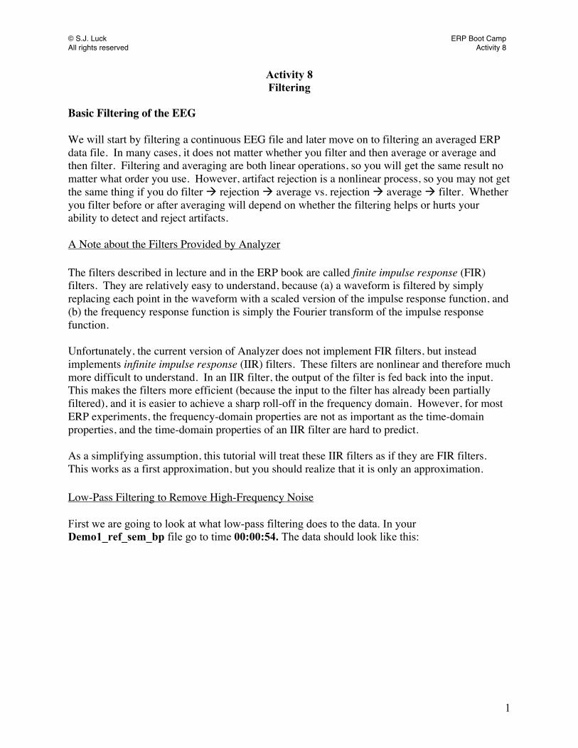
© S.J. Luck ERP Boot Camp All rights reserved Activity 8
1
Activity 8 Filtering
Basic Filtering of the EEG We will start by filtering a continuous EEG file and later move on to filtering an averaged ERP data file. In many cases, it does not matter whether you filter and then average or average and then filter. Filtering and averaging are both linear operations, so you will get the same result no matter what order you use. However, artifact rejection is a nonlinear process, so you may not get the same thing if you do filter rejection average vs. rejection average filter. Whether you filter before or after averaging will depend on whether the filtering helps or hurts your ability to detect and reject artifacts. A Note about the Filters Provided by Analyzer The filters described in lecture and in the ERP book are called finite impulse response (FIR) filters. They are relatively easy to understand, because (a) a waveform is filtered by simply replacing each point in the waveform with a scaled version of the impulse response function, and (b) the frequency response function is simply the Fourier transform of the impulse response function. Unfortunately, the current version of Analyzer does not implement FIR filters, but instead implements infinite impulse response (IIR) filters. These filters are nonlinear and therefore much more difficult to understand. In an IIR filter, the output of the filter is fed back into the input. This makes the filters more efficient (because the input to the filter has already been partially filtered), and it is easier to achieve a sharp roll-off in the frequency domain. However, for most ERP experiments, the frequency-domain properties are not as important as the time-domain properties, and the time-domain properties of an IIR filter are hard to predict. As a simplifying assumption, this tutorial will treat these IIR filters as if they are FIR filters. This works as a first approximation, but you should realize that it is only an approximation. Low-Pass Filtering to Remove High-Frequency Noise First we are going to look at what low-pass filtering does to the data. In your Demo1_ref_sem_bp file go to time 00:00:54. The data should look like this:

© S.J. Luck ERP Boot Camp All rights reserved Activity 8
2
FP1FzF3F7T7C3CzP1P3P5P7P9PO7PO3O1IzFp2F4F8T8C4PzP2P4P6P8P10PO8PO4POzOzO2EXG1EXG2EXG3EXG4EXG5EXG6HEOGR-LVEOGL-U
17 5 42 5
50 µV
00:00:54 unfiltered As you can see, there is some high frequency noise, probably associated with muscle activity. As our first step, we will filter out these high frequencies with various filter settings. Go to Transformations > Artifact Rejection/Reduction > Data Filtering> IIR Filters. You will see four options: low cutoff, high cutoff, notch, and individual channel filters. NOTE: Low cutoff and High cutoff should not be confused with low-pass and high-pass filters. When we use a low-pass filter, we remove high-frequency noise (in other words, we let the low frequencies pass and filter out the high frequencies). To do this, we must set a high cutoff where everything above the cutoff will be filtered out. Try a low-pass filter with a high cutoff of 100 Hz and a roll-off of 12 dB/octave. Rename this node 100Hz 12dB. It should not look very different from the unfiltered data. To see this, you can drag the icon for the original node (Demo1_ref_bp) onto the data display window, which will cause the original data to be plotted along with the filtered data. The filtering has such little effect that it’s hard to see any difference between the filtered and
unfiltered data. Change the display interval to 0.5 seconds (click on the button) and scroll over to 00:00:58.5. Now you can see the differences, but they are still very small. Go back to the unfiltered data and try the same low-pass filter cutoff, except use a roll-off of 48 dB/octave and rename the file 100Hz 48dB. This filter has the same half-power cutoff as the
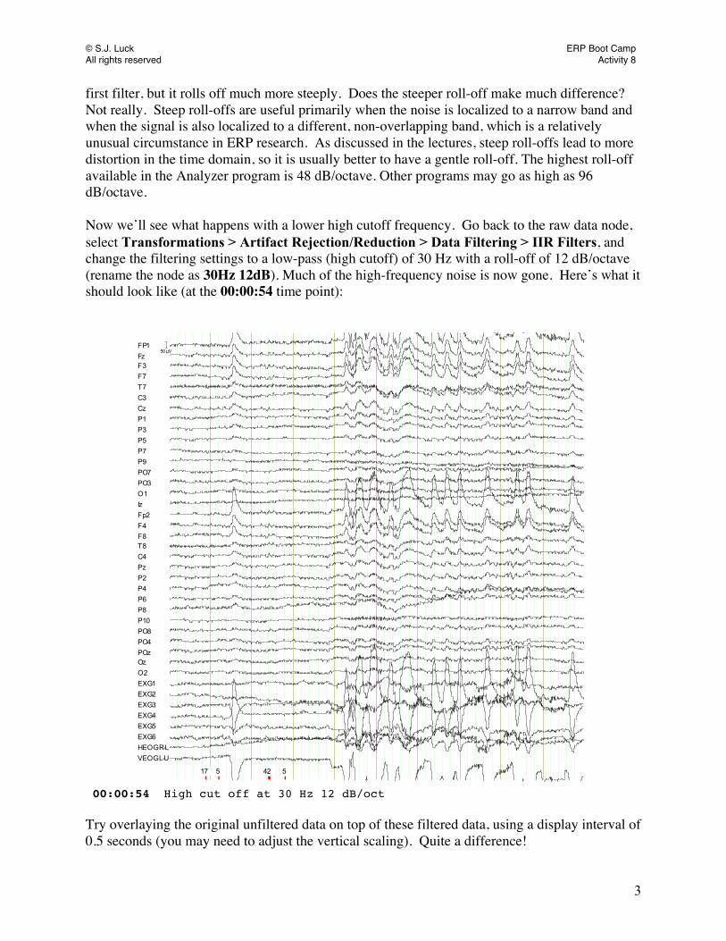
© S.J. Luck ERP Boot Camp All rights reserved Activity 8
3
first filter, but it rolls off much more steeply. Does the steeper roll-off make much difference? Not really. Steep roll-offs are useful primarily when the noise is localized to a narrow band and when the signal is also localized to a different, non-overlapping band, which is a relatively unusual circumstance in ERP research. As discussed in the lectures, steep roll-offs lead to more distortion in the time domain, so it is usually better to have a gentle roll-off. The highest roll-off available in the Analyzer program is 48 dB/octave. Other programs may go as high as 96 dB/octave. Now we’ll see what happens with a lower high cutoff frequency. Go back to the raw data node, select Transformations > Artifact Rejection/Reduction > Data Filtering > IIR Filters, and change the filtering settings to a low-pass (high cutoff) of 30 Hz with a roll-off of 12 dB/octave (rename the node as 30Hz 12dB). Much of the high-frequency noise is now gone. Here’s what it should look like (at the 00:00:54 time point):
FP1FzF3F7T7C3CzP1P3P5P7P9PO7PO3O1IzFp2F4F8T8C4PzP2P4P6P8P10PO8PO4POzOzO2EXG1EXG2EXG3EXG4EXG5EXG6HEOGR-LVEOGL-U
17 5 42 5
50 µV
00:00:54 High cut off at 30 Hz 12 dB/oct Try overlaying the original unfiltered data on top of these filtered data, using a display interval of 0.5 seconds (you may need to adjust the vertical scaling). Quite a difference!
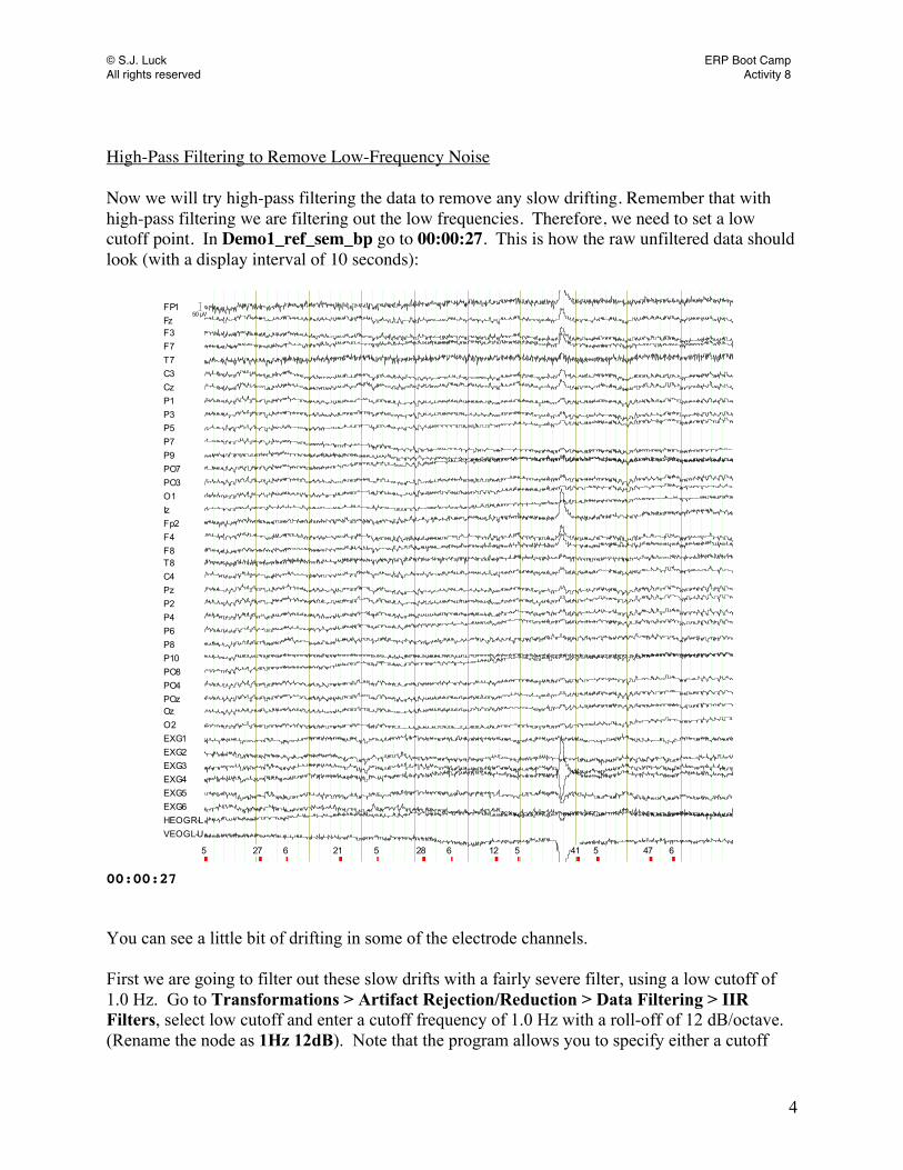
© S.J. Luck ERP Boot Camp All rights reserved Activity 8
4
High-Pass Filtering to Remove Low-Frequency Noise Now we will try high-pass filtering the data to remove any slow drifting. Remember that with high-pass filtering we are filtering out the low frequencies. Therefore, we need to set a low cutoff point. In Demo1_ref_sem_bp go to 00:00:27. This is how the raw unfiltered data should look (with a display interval of 10 seconds):
FP1FzF3F7T7C3CzP1P3P5P7P9PO7PO3O1IzFp2F4F8T8C4PzP2P4P6P8P10PO8PO4POzOzO2EXG1EXG2EXG3EXG4EXG5EXG6HEOGR-LVEOGL-U
5 27 6 21 5 28 6 12 5 41 5 47 6
50 µV
00:00:27 You can see a little bit of drifting in some of the electrode channels. First we are going to filter out these slow drifts with a fairly severe filter, using a low cutoff of 1.0 Hz. Go to Transformations > Artifact Rejection/Reduction > Data Filtering > IIR Filters, select low cutoff and enter a cutoff frequency of 1.0 Hz with a roll-off of 12 dB/octave. (Rename the node as 1Hz 12dB). Note that the program allows you to specify either a cutoff
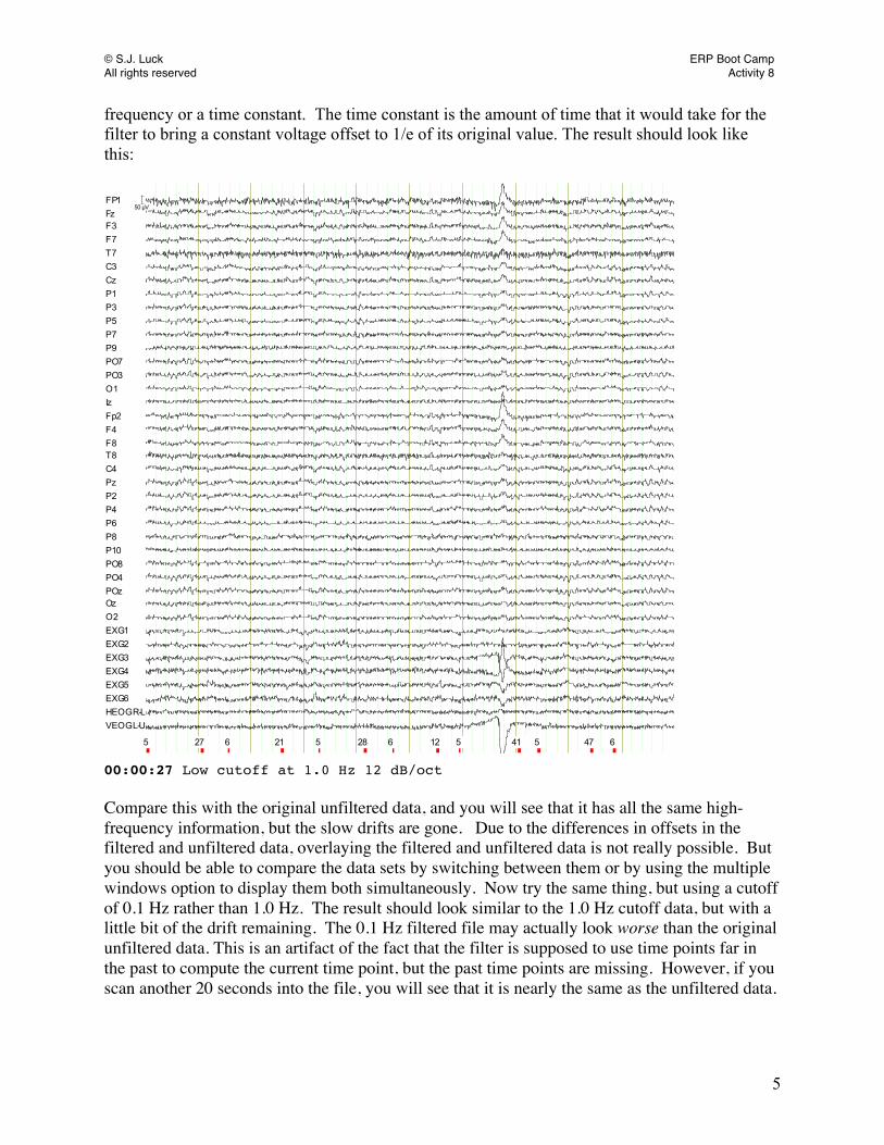
© S.J. Luck ERP Boot Camp All rights reserved Activity 8
5
frequency or a time constant. The time constant is the amount of time that it would take for the filter to bring a constant voltage offset to 1/e of its original value. The result should look like this: FP1FzF3F7T7C3CzP1P3P5P7P9PO7PO3O1IzFp2F4F8T8C4PzP2P4P6P8P10PO8PO4POzOzO2EXG1EXG2EXG3EXG4EXG5EXG6HEOGR-LVEOGL-U
5 27 6 21 5 28 6 12 5 41 5 47 6
50 µV
00:00:27 Low cutoff at 1.0 Hz 12 dB/oct Compare this with the original unfiltered data, and you will see that it has all the same high-frequency information, but the slow drifts are gone. Due to the differences in offsets in the filtered and unfiltered data, overlaying the filtered and unfiltered data is not really possible. But you should be able to compare the data sets by switching between them or by using the multiple windows option to display them both simultaneously. Now try the same thing, but using a cutoff of 0.1 Hz rather than 1.0 Hz. The result should look similar to the 1.0 Hz cutoff data, but with a little bit of the drift remaining. The 0.1 Hz filtered file may actually look worse than the original unfiltered data. This is an artifact of the fact that the filter is supposed to use time points far in the past to compute the current time point, but the past time points are missing. However, if you scan another 20 seconds into the file, you will see that it is nearly the same as the unfiltered data.

© S.J. Luck ERP Boot Camp All rights reserved Activity 8
6
As a final step, we will combine low-pass and high-pass filtering into a single step, which is known as a band-pass filter. Select the unfiltered Demo1_ref_sem_bp node, go to Transformations > Artifact Rejection/Reduction > Data Filtering > IIR Filters, and select both the low cutoff of 0.1 Hz with a roll-off of 12 dB/octave and a high cutoff of 30 Hz with a roll-off of 12 dB/octave. The result should look like the screenshot below, with minimal low-frequency drift and minimal high-frequency noise. Filtering is a linear operation, so this should be equivalent to filtering once with a high-pass filter at 0.1 Hz, and then filtering the filtered file a second time with a low-pass filter at 30 Hz. Try this and verify that it looks the same.
FP1FzF3F7T7C3CzP1P3P5P7P9PO7PO3O1IzFp2F4F8T8C4PzP2P4P6P8P10PO8PO4POzOzO2EXG1EXG2EXG3EXG4EXG5EXG6HEOGR-LVEOGL-U
31 5 42 21 5 12 5 11 5 22 5 41 5
50 µV
CMS in RangeStart EpochActiveTwo MK2ActiveTwo MK2CMS in Range 56
00:00:00 Filtering and Spectral Analysis of Averaged Waveforms We will now filter the averaged data that you created to look at the C1, so go back to the Avg_Upper file. It should look like this:
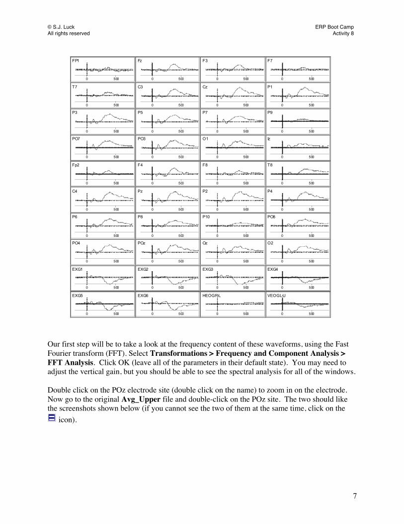
© S.J. Luck ERP Boot Camp All rights reserved Activity 8
7
FP1 Fz F3 F7
T7 C3 Cz P1
P3 P5 P7 P9
PO7 PO3 O1 Iz
Fp2 F4 F8 T8
C4 Pz P2 P4
P6 P8 P10 PO8
PO4 POz Oz O2
EXG1 EXG2 EXG3 EXG4
EXG5 EXG6 HEOGR-L VEOGL-U
0 500 0 500 0 500 0 500
0 500 0 500 0 500 0 500
0 500 0 500 0 500 0 500
0 500 0 500 0 500 0 500
0 500 0 500 0 500 0 500
0 500 0 500 0 500 0 500
0 500 0 500 0 500 0 500
0 500 0 500 0 500 0 500
0 500 0 500 0 500 0 500
0 500 0 500 0 500 0 500
Our first step will be to take a look at the frequency content of these waveforms, using the Fast Fourier transform (FFT). Select Transformations > Frequency and Component Analysis > FFT Analysis. Click OK (leave all of the parameters in their default state). You may need to adjust the vertical gain, but you should be able to see the spectral analysis for all of the windows. Double click on the POz electrode site (double click on the name) to zoom in on the electrode. Now go to the original Avg_Upper file and double-click on the POz site. The two should like the screenshots shown below (if you cannot see the two of them at the same time, click on the
icon).

© S.J. Luck ERP Boot Camp All rights reserved Activity 8
8
POz
-200 -100 0 100 200 300 400 500 600 700
-10
-5
0
5
10
Sub-Delta Delta Theta Alpha Beta
POz
0 20 40 60 80 100 1200.00
0.10
0.20
0.30
0.40
0.50
0.60
0.70
The first thing to notice is the spike at 60 Hz in the frequency-domain plot. If you look closely at the time-domain plot, you should be able to count 6 little peaks in every 100 ms period (e.g.,
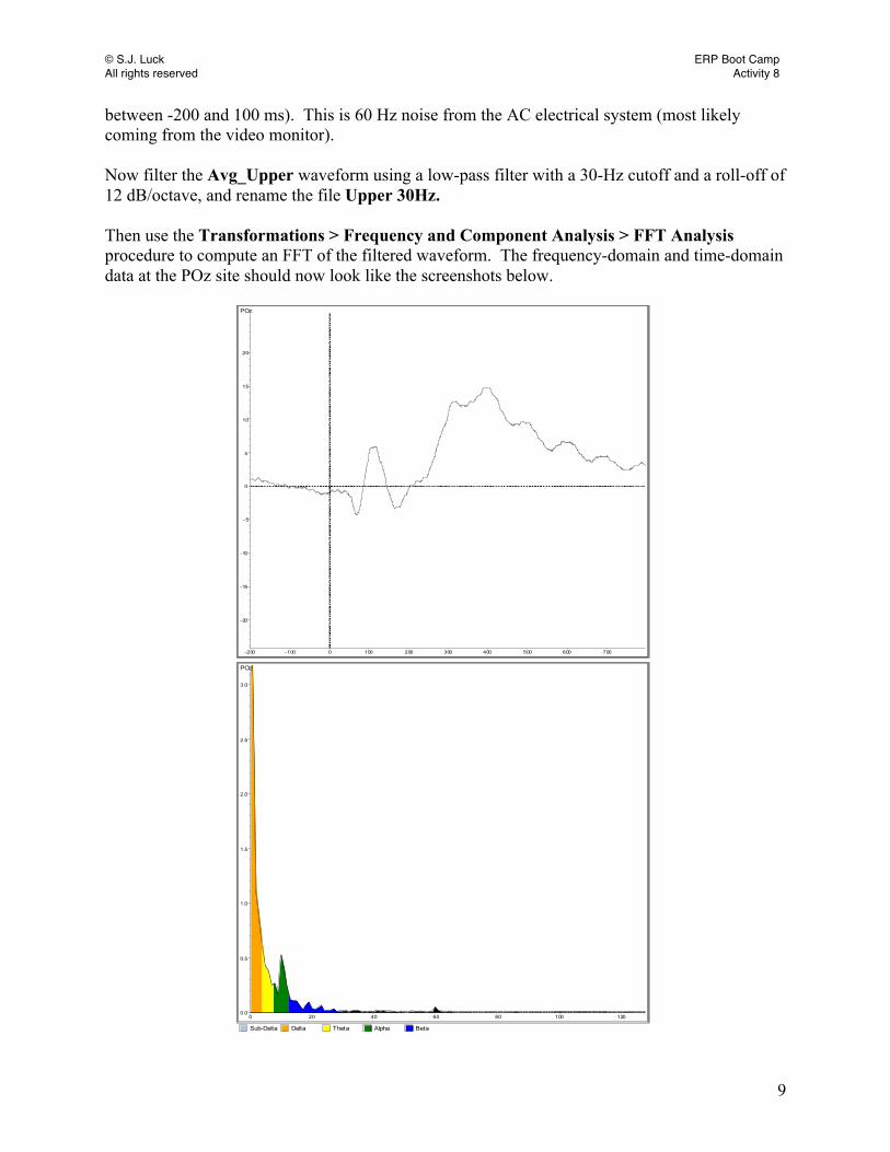
© S.J. Luck ERP Boot Camp All rights reserved Activity 8
9
between -200 and 100 ms). This is 60 Hz noise from the AC electrical system (most likely coming from the video monitor). Now filter the Avg_Upper waveform using a low-pass filter with a 30-Hz cutoff and a roll-off of 12 dB/octave, and rename the file Upper 30Hz. Then use the Transformations > Frequency and Component Analysis > FFT Analysis procedure to compute an FFT of the filtered waveform. The frequency-domain and time-domain data at the POz site should now look like the screenshots below.
POz
-200 -100 0 100 200 300 400 500 600 700
-20
-15
-10
-5
0
5
10
15
20
Sub-Delta Delta Theta Alpha Beta
POz
0 20 40 60 80 100 1200.0
0.5
1.0
1.5
2.0
2.5
3.0

© S.J. Luck ERP Boot Camp All rights reserved Activity 8
10
Note that the peak at 60-Hz in the FFT is reduced (but not entirely eliminated), and the little high-frequency peaks in the time-domain waveform are largely gone in the filtered data. Why isn’t the 60-Hz activity completely eliminated given that the filter cutoff was 30 Hz? To understand this, we need to describe some terminology. First, let’s consider the cutoff frequency. When filtering in Analyzer, the cutoff that you specify for the filter is the half-power cutoff. In other words, that means that the power at the cutoff frequency you specify will be half of the power in the unfiltered data. Other software programs use a half-amplitude cutoff instead of a half-power cutoff. This would mean that the amplitude at the cutoff frequency you specify will be half of the amplitude at 0 Hz. Remember that power is amplitude squared. Although counterintuitive, a half-amplitude cutoff of 30 Hz would be more severe than a half-power cutoff of 30 Hz. This is true because a reduction in amplitude by a factor of 0.5 is equal to a reduction in power by a factor of 0.52 = 0.25. Thus, a half-power cutoff at 30 Hz means that the amplitude is reduced by only 25% at 30 Hz. The roll-off of a filter is usually specified in dB per octave. An octave is a doubling of frequency. Decibel (dB) is a logarithmic scale for representing magnitude. A 3 dB decrease in magnitude corresponds to a decrease of 50% in power, and a 6 dB decrease in magnitude corresponds to a 50% decrease in amplitude. A roll-off of 3 dB/octave means that the power drops by 50% every time the frequency doubles. Because dB is a logarithmic scale, a drop of 9 dB is a drop in power of 50% of 50% of 50% (or 0.53). Thus, a roll-off of 12 dB/octave means that the power will decline from X at a given frequency to 0.54X (6.25% of X) at twice that frequency. In terms of amplitude, this would be a drop of 6 dB and then another drop of 6 dB, or a drop in amplitude to 0.52X (or 25% of X). Now we can understand why the 60-Hz activity is not completely eliminated given that the filter cutoff was 30 Hz. We’ve selected a roll-off of 12 dB/octave, which means that the magnitude is reduced by 3 dB at 30 Hz and will be reduced by another 12 dB when the frequency doubles to 60 Hz. Thus, the magnitude will be reduced by 15 dB at 60 Hz in the filtered data relative to the unfiltered data. This is a reduction in power to 0.55, and a reduction in amplitude to sqrt(0.55) or approximately 0.18. Thus, we have reduced the amplitude by 82% at 60 Hz with this filter. Now we will try high-pass filtering (removing the low frequencies) from the Avg_Upper node. Select this node and do Transformations > Artifact Rejection/Reduction > Data Filtering > IIR Filters with a high-pass filter (low cutoff) of 1.0 Hz with a roll-off of 12 dB/octave, and rename the file Upper 1Hz. If you enlarge the POz scalp site, you should see something like the screen shot below.
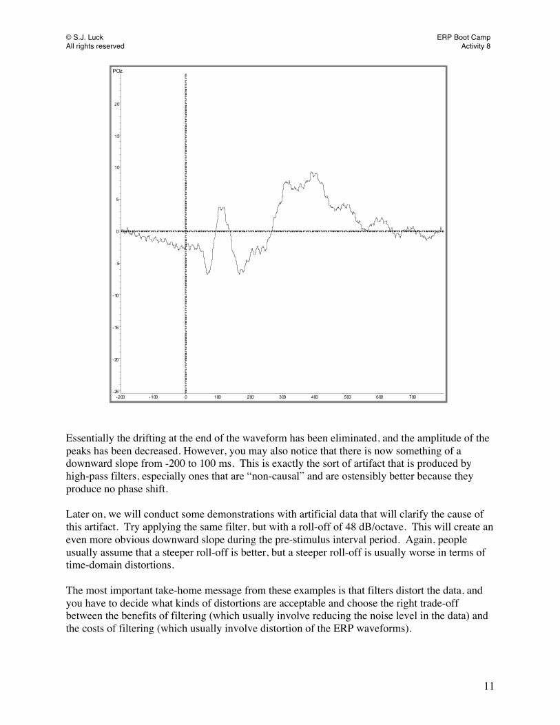
© S.J. Luck ERP Boot Camp All rights reserved Activity 8
11
POz
-200 -100 0 100 200 300 400 500 600 700-25
-20
-15
-10
-5
0
5
10
15
20
Essentially the drifting at the end of the waveform has been eliminated, and the amplitude of the peaks has been decreased. However, you may also notice that there is now something of a downward slope from -200 to 100 ms. This is exactly the sort of artifact that is produced by high-pass filters, especially ones that are “non-causal” and are ostensibly better because they produce no phase shift. Later on, we will conduct some demonstrations with artificial data that will clarify the cause of this artifact. Try applying the same filter, but with a roll-off of 48 dB/octave. This will create an even more obvious downward slope during the pre-stimulus interval period. Again, people usually assume that a steeper roll-off is better, but a steeper roll-off is usually worse in terms of time-domain distortions. The most important take-home message from these examples is that filters distort the data, and you have to decide what kinds of distortions are acceptable and choose the right trade-off between the benefits of filtering (which usually involve reducing the noise level in the data) and the costs of filtering (which usually involve distortion of the ERP waveforms).

© S.J. Luck ERP Boot Camp All rights reserved Activity 8
12
Our final example with this file will be to apply a notch filter. Select Avg_Upper and then select Transformations > Artifact Rejection/Reduction > Data Filtering > IIR Filters. This time, make sure that low cutoff and high cutoff are disabled. Check the Enable option under Notch. Make sure that the frequency is at 60 Hz and press OK. The result at the POz site should look like the figure below. If you compare this to the original waveform, you will see that the 60 Hz oscillations have been largely removed, but some higher-frequency noise still remains, along with all of the lower frequencies. Keep in mind that, although this looks nice, notch filters can seriously distort your data, and they should be used only under rare conditions (such as when there is so much 60 Hz noise in the EEG during data collection that you cannot see if there are other artifacts or noise sources in the data).
POz
-200 -100 0 100 200 300 400 500 600 700
-20
-15
-10
-5
0
5
10
15
20
Viewing the Impulse Response Function of a Filter As described in the book and the lectures, the key to understanding the time-domain distortions produced by filters is to view them in the time domain rather than in the frequency domain. That is, you should look at the impulse response function (IRF) of the filters you are using. You can think of filtering as a process that replaces each point in the original waveform with a copy of the IRF, scaled by the height of the current point (this is the mathematical process of convolution). Alternatively, you can assess the effects of the filter on the filtered value at the current time point

© S.J. Luck ERP Boot Camp All rights reserved Activity 8
13
by reversing the IRF in time; the current value equals all of the other points in the waveform scaled by this reversed IRF. The bad news is that most ERP analysis packages do not show you the IRFs of the filters. The good news is that it is trivially easy to figure out a filter’s IRF. An IRF is simply the response (output) of the filter when the input is an impulse (a momentary voltage spike). Thus, all you need to do to see the IRF is create a fake data file in which the waveform is zero at all points except at time zero, where the voltage should be 1.0 µV. We’ve already done this for you. The text file is called artificial waveforms (you can find it at C:\Bootcamp_Analyzer2\Documentation), and you can use it as a starting point for making new artificial waveforms (although you might want to try reducing the sampling rate first-–this file contains a large number of points). If you want to try doing this, you might find it easiest to use Excel to create the values and then paste them into the text file. We have already imported this file into Analyzer and it is called Demo3 -- Raw Data. When you select this node, you will see that it actually has three artificial waveforms, one in each of three channels. You may need to adjust the scaling a bit so it looks like the figure below.
IMPULSE
SINE
WAVE
-200 -100 0 100 200 300 400 500 600 700-1.5
-1.0
-0.5
0.0
0.5
1.0
-200 -100 0 100 200 300 400 500 600 700-1.5
-1.0
-0.5
0.0
0.5
1.0
-200 -100 0 100 200 300 400 500 600 700-1.5
-1.0
-0.5
0.0
0.5
1.0

© S.J. Luck ERP Boot Camp All rights reserved Activity 8
14
The first channel is the impulse (note, however, that it does not look like a single-point impulse because of the interpolation caused by the graphics engine). The second channel is a single cycle of a 5.0 Hz sine wave. The third channel is a simulated noise-free ERP waveform, with P1, N1, and P3 waves (created by summing together three Gaussians of different sizes, widths, and starting points). It is useful to see the effects of a filter on all three of these. The impulse shows you the IRF; the sine wave helps you see the effects of the filter on the onset and offset of the waveform; the simulated ERP helps you to see the effects of the filter on a realistic waveform (although you may eventually need to create a different waveform that is more similar to what you see in your own experiments). Let’s start by selecting Demo3 -- Raw Data and clicking on Transformations > Artifact Rejection/Reduction > Data Filtering > IIR Filters. Select a low pass filter with a high cutoff of 10 Hz and a roll-off of 12 dB/octave, and then rename the filtered data node 10 Hz 12 dB. Now click and drag the Demo3 -- Raw Data file on top of the filtered data. This will allow you to directly compare the filtered and unfiltered data. The result is shown in the screenshot below.
IMPULSE 10hz 12db
SINE10hz 12db
WAVE10hz 12db
-200 -100 0 100 200 300 400 500 600 700-1.5
-1.0
-0.5
0.0
0.5
1.0
-200 -100 0 100 200 300 400 500 600 700-1.5
-1.0
-0.5
0.0
0.5
1.0
-200 -100 0 100 200 300 400 500 600 700-1.5
-1.0
-0.5
0.0
0.5
1.0

© S.J. Luck ERP Boot Camp All rights reserved Activity 8
15
The first thing to note is the IMPULSE channel, which overlays the impulse and the IRF. The IRF is so small that it’s hard to see, so you might want to temporarily increase the vertical gain using the up arrow (this is because all of the values in the IRF must sum to 1.0, so each value is pretty small). Note that the impulse response function looks something like a triangle around the impulse. This means that the filtered value at a given time point mostly reflects the original value at that time point, with a contribution from nearby time points that decreases over time. That’s a good thing, because it means that the filtered value at a given time point mostly reflects that time point and nearby time points. It also means that the original value at one point in time will spread to nearby points in time in the filtered waveform, but with a decreasing effect over time. This can be seen in both the SINE and WAVE channels, where the filtered waveform begins before and ends after the unfiltered waveform. There is also a decrease in the amplitudes of some of the peaks in these waveforms, which reflects the fact that they contain some power in the time range that is being filtered by this particular filter. Now let’s take a look at the Fourier transforms of the three unfiltered waveforms. Go to Demo3 -- Raw Data, select Transformations > Frequency and Component Analysis > FFT Analysis, choose the power (µV2) option, and rename the output as artificial fft. The Fourier transforms are shown in the screen shots below; you will first want to maximize each channel and adjust the vertical scale so that you can see things properly for each channel.
Sub-Delta Delta Theta Alpha Beta
IMPULSE
SINE
WAVE
0 20 40 60 80 100 1200.000
0.005
0.010
0.015
0.020
0 20 40 60 80 100 1200.000
0.005
0.010
0.015
0.020
0 20 40 60 80 100 1200.000
0.005
0.010
0.015
0.020
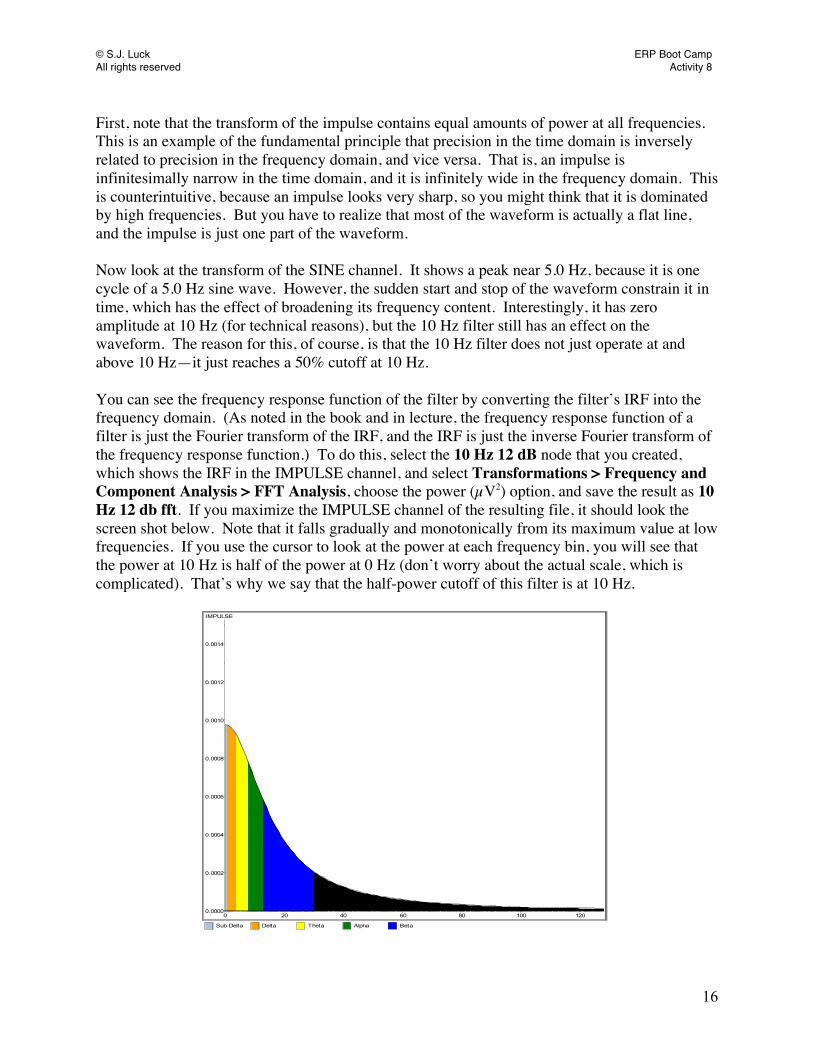
© S.J. Luck ERP Boot Camp All rights reserved Activity 8
16
First, note that the transform of the impulse contains equal amounts of power at all frequencies. This is an example of the fundamental principle that precision in the time domain is inversely related to precision in the frequency domain, and vice versa. That is, an impulse is infinitesimally narrow in the time domain, and it is infinitely wide in the frequency domain. This is counterintuitive, because an impulse looks very sharp, so you might think that it is dominated by high frequencies. But you have to realize that most of the waveform is actually a flat line, and the impulse is just one part of the waveform. Now look at the transform of the SINE channel. It shows a peak near 5.0 Hz, because it is one cycle of a 5.0 Hz sine wave. However, the sudden start and stop of the waveform constrain it in time, which has the effect of broadening its frequency content. Interestingly, it has zero amplitude at 10 Hz (for technical reasons), but the 10 Hz filter still has an effect on the waveform. The reason for this, of course, is that the 10 Hz filter does not just operate at and above 10 Hz—it just reaches a 50% cutoff at 10 Hz. You can see the frequency response function of the filter by converting the filter’s IRF into the frequency domain. (As noted in the book and in lecture, the frequency response function of a filter is just the Fourier transform of the IRF, and the IRF is just the inverse Fourier transform of the frequency response function.) To do this, select the 10 Hz 12 dB node that you created, which shows the IRF in the IMPULSE channel, and select Transformations > Frequency and Component Analysis > FFT Analysis, choose the power (µV2) option, and save the result as 10 Hz 12 db fft. If you maximize the IMPULSE channel of the resulting file, it should look the screen shot below. Note that it falls gradually and monotonically from its maximum value at low frequencies. If you use the cursor to look at the power at each frequency bin, you will see that the power at 10 Hz is half of the power at 0 Hz (don’t worry about the actual scale, which is complicated). That’s why we say that the half-power cutoff of this filter is at 10 Hz.
Sub-Delta Delta Theta Alpha Beta
IMPULSE
0 20 40 60 80 100 1200.0000
0.0002
0.0004
0.0006
0.0008
0.0010
0.0012
0.0014
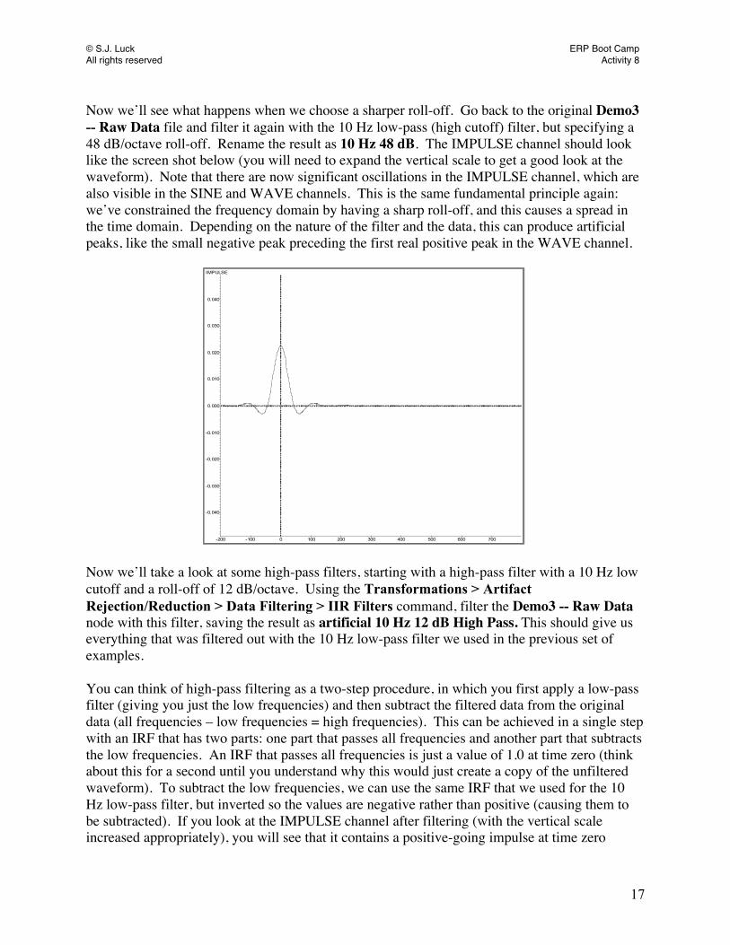
© S.J. Luck ERP Boot Camp All rights reserved Activity 8
17
Now we’ll see what happens when we choose a sharper roll-off. Go back to the original Demo3 -- Raw Data file and filter it again with the 10 Hz low-pass (high cutoff) filter, but specifying a 48 dB/octave roll-off. Rename the result as 10 Hz 48 dB. The IMPULSE channel should look like the screen shot below (you will need to expand the vertical scale to get a good look at the waveform). Note that there are now significant oscillations in the IMPULSE channel, which are also visible in the SINE and WAVE channels. This is the same fundamental principle again: we’ve constrained the frequency domain by having a sharp roll-off, and this causes a spread in the time domain. Depending on the nature of the filter and the data, this can produce artificial peaks, like the small negative peak preceding the first real positive peak in the WAVE channel.
IMPULSE
-200 -100 0 100 200 300 400 500 600 700
-0.040
-0.030
-0.020
-0.010
0.000
0.010
0.020
0.030
0.040
Now we’ll take a look at some high-pass filters, starting with a high-pass filter with a 10 Hz low cutoff and a roll-off of 12 dB/octave. Using the Transformations > Artifact Rejection/Reduction > Data Filtering > IIR Filters command, filter the Demo3 -- Raw Data node with this filter, saving the result as artificial 10 Hz 12 dB High Pass. This should give us everything that was filtered out with the 10 Hz low-pass filter we used in the previous set of examples. You can think of high-pass filtering as a two-step procedure, in which you first apply a low-pass filter (giving you just the low frequencies) and then subtract the filtered data from the original data (all frequencies – low frequencies = high frequencies). This can be achieved in a single step with an IRF that has two parts: one part that passes all frequencies and another part that subtracts the low frequencies. An IRF that passes all frequencies is just a value of 1.0 at time zero (think about this for a second until you understand why this would just create a copy of the unfiltered waveform). To subtract the low frequencies, we can use the same IRF that we used for the 10 Hz low-pass filter, but inverted so the values are negative rather than positive (causing them to be subtracted). If you look at the IMPULSE channel after filtering (with the vertical scale increased appropriately), you will see that it contains a positive-going impulse at time zero

© S.J. Luck ERP Boot Camp All rights reserved Activity 8
18
(partially obscured by the line marking time zero), surrounded by an inverted version of the IRF that we saw with the 10 Hz low-pass filter (see screen shot below).
IMPULSE
-200 -100 0 100 200 300 400 500 600 700
-0.15
-0.10
-0.05
0.00
0.05
0.10
0.15
It would be very unusual to use a high-pass filter with such a high cutoff, so lets take a look at a more realistic example with a 1.0 Hz cutoff (do everything the same as for the 10 Hz cutoff, but use a 1.0 Hz cutoff instead). As shown in the screen shot below, it is now difficult to see the negative portion in the IMPULSE channel; this portion is so broad that it looks like a flat line. However, you can still see it if you expand the scale sufficiently. And you can see the distortions this filter produces in the SINE and WAVE channels. Note, in particular, the downward slope of the prestimulus baseline in the WAVE channel.

© S.J. Luck ERP Boot Camp All rights reserved Activity 8
19
IMPULSE
SINE
WAVE
-200 -100 0 100 200 300 400 500 600 700
-0.6
-0.4
-0.2
0.0
0.2
0.4
0.6
-200 -100 0 100 200 300 400 500 600 700
-0.6
-0.4
-0.2
0.0
0.2
0.4
0.6
-200 -100 0 100 200 300 400 500 600 700-0.8
-0.6
-0.4
-0.2
0.0
0.2
0.4
0.6
This is similar to what we saw when we applied this same filter to the Avg_Upper file in the previous set of examples. Now we can see why this happens. Remember that filtering is equivalent to replacing each point from the unfiltered waveform with a scaled version of the IRF. Thus, for a high-pass filter, each positive point in the waveform is replaced by a positive impulse at the time of that point (which just copies the voltage at that point) and negative values at a broad range of surrounding points. Similarly, each negative point is replaced by a negative impulse at the time of that point and positive values at a broad range of surrounding points. The small positive peak and large positive peak in the unfiltered WAVE waveform together cause relatively large negative voltages to be spread to the surrounding time points, and these outweigh the positive voltages that are spread around the negative peak. Consequently, the overall effect is a negative set of voltages that gradually fade away toward the beginning and end of the epoch. Try the same thing with a 48 dB/octave roll-off. You will see an even more extreme downward slope in the baseline period of the WAVE channel. Filtering Your Own Data Now that you have seen how filters work, you should practice applying them to your own data. Try all of these different kinds of filters, using different cutoff frequencies and roll-offs. Also, try filtering the EEG and then averaging and comparing this to averaging and then filtering (without any artifact rejection). Try it with artifact rejection as well. Does the filtering make it easier or more difficult to do artifact rejection? This will depend on the specific filter you use and the nature of your artifacts.
Top Related