


Languages
Pages
Legal


THE AMERICAN SOCIETY OF MECHANICAL ENGINEERS345 E. 47th St., New York, N.Y. 10017
The Society shall not be responsible for statements or opinions advanced inpapers or discussion at meetings of the Society or of its Divisions or Sections,or printed in its publications. Discussion is printed only if the paper is pub-lished in an ASME Journal. Papers are available from ASME for 15 monthsafter the meeting.
Printed in U.S.A.
93-GT-92
THREE DIMENSIONAL TIME-MARCHING INVISCID ANDVISCOUS SOLUTIONS FOR UNSTEADY FLOWS
AROUND VIBRATING BLADES
L. He and J. D. DentonWhittle Laboratory
Cambridge UniversityCambridge, United Kingdom
AbstractA 3-dimensional non-linear time-marching method of solving
the thin-layer Navier-Stokes equations in a simplified form has been
developed for blade flutter calculations. The discretization of the
equations is made using the cell-vertex finite volume scheme in space
and the 4-stage Runge-Kutta scheme in time. Calculations are carried
out in a single-blade-passage domain and the phase-shifted periodic
condition is implemented by using the shape correction method. The
3-D unsteady Euler solution is obtained at conditions of zero
viscosity, and is validated against a well-established 3-D semi-
analytical method. For viscous solutions, the time-step limitation on
the explicit temporal discretization scheme is effectively relaxed by
using a time-consistent two-grid time-marching technique. A
transonic rotor blade passage flow (with tip-leakage) is calculated
using the present 3-D unsteady viscous solution method. Calculated
steady flow results agree well with the corresponding experiment and
with other calculations. Calculated unsteady loadings due to
oscillations of the rotor blades reveal some notable 3-D viscous flow
features. The feasibility of solving the simplified thin-layer Navier-
Stokes solver for oscillating blade flows at practical conditions is
demonstrated.
Nomenclature
C Chord length
Cpi unsteady pressure coefficient
dA differential area element with unit outward normal vector
dV differential volume element
E internal energy
f frequency
n„ the unit vectors in x direction
static pressure
radial coordinate
S span
S, --- viscous terms in a body force form
U --- primitive flow variable
velocity in x direction
--- absolute velocity at inlet
velocity in 8 direction
w -- velocity in radial direction
axial coordinate
Cm --- turbulence eddy viscosity
laminar viscosity coefficient
0 circumferential coordinate
p density
inter blade phase angle
shear stress
angular frequency
Superscript
n --- index of time step
Subscript
time averaged
mg --- moving grid
order of the Fourier component
on walls
IntroductionPredictions of unsteady flows around vibrating blades are
essential for turbomachinery blade flutter predictions. Numerical
methods of calculating unsteady flows through vibrating blades are
currently under active development. Most of the methods available
Presented at the International Gas Turbine and Aeroengine Congress and ExpositionCincinnati, Ohio May 24-27, 1993
This paper has been accepted for publication in the Transactions of the ASMEDiscussion of it will be accepted at ASME Headquarters until September 30,1993
Copyright © 1993 by ASME
Downloaded From: http://proceedings.asmedigitalcollection.asme.org/ on 06/04/2018 Terms of Use: http://www.asme.org/about-asme/terms-of-use
are for a 2-dimensional model. Notable examples are the work by
Verdon and Caspar (1982) and Whitehead (1982). Under practical
turbomachinery working conditions, three dimensional effects are
important and need to be modelled. Calculations of 3-dimensional
unsteady flows are usually simplified by assuming that a flow field
would behave in a 2-dimensional fashion at each spanwise section,so the strip method (i.e. performing 2-D calculations at each section)
can be used. It has been demonstrated that the strip theory can lead to
serious errors for blade flutter calculations (e.g. Namba, 1987).
For simple 3-D blade geometries (e.g. flat plate cascade) at
purely subsonic or supersonic flow conditions, fully 3-D inviscid
solutions for oscillating blade flows can be efficiently and accurately
obtained by using semi-analytical theories. Examples of this kind are
those by Namba (1976, 1987) and Chi (1991). These semi-analytical
methods can provide some basic insight into 3-D effects on blade
aeroelastic behaviours, but their capability in predicting blade flutter
under practical flow conditions is rather limited.
Recently three dimensional numerical methods for blade flutter
calculations have begun to emerge. 3-D inviscid Euler solutions have
been developed by Giles (1991) and Hall and Lorence (1992) using
a time-linearized model, and by Gerolymos (1992) using a time-
marching method. So far no work on 3-D unsteady viscous flow
solutions for blade flutter calculations has been reported.
The objective of the present work is to develop a nonlinear time-
marching viscous flow solution method for blade flutter calculations.
The major effort is focused on enhancing solution efficiency which is
believed to be a very important factor affecting the feasibility of
unsteady time-marching solvers for industrial use. For the phase-
shifted periodic boundary condition, the "Shape Correction" method
developed for the previous 2-D Euler solver (He, 1989) is extended
to the present 3-D solution to save computer storage. Another feature
of the present work is that the time-step limitation on the explicit
time-marching scheme, is effectively relaxed by using a time-
consistent two-grid technique.
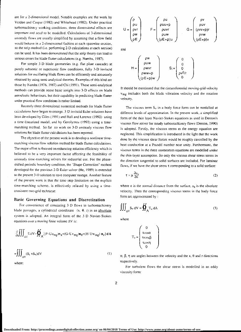
Basic Governing Equations and DiscretizationFor convenience of simulating 3-D flows in turbomachinery
blade passages, a cylindrical coordinate (x, 0, r) in an absolute
system is adopted. An integral form of the 3-D Navier-Stokes
equations over a moving finite volume AV is:
(p pu pvpu puu+p puv
U = pvr F puvr G = (pvv+p)r
Pw puw pvw
E ) (pE+p)u (pE+p)v 1and
r pw
puw(
0H pwvr
pww+p
Si = 0pv2/r
(pE+p)w
\ 0 )
It should be mentioned that the circumferential moving-grid velocity
v mg includes both the blade vibration velocity and the rotation
velocity.
The viscous term S v in a body force form can be modelled at
different levels of approximation. In the present work, a simplified
form of the thin-layer Navier-Stokes equations as used in Denton's
viscous flow solver for steady turbomachinery flows (Denton, 1990)
is adopted. Firstly, the viscous terms in the energy equation are
neglected. This simplification is introduced in the light that the work
done by the viscous shear forces would be roughly cancelled by the
heat conduction at a Prandtl number near unity. Furthermore, the
viscous terms in the three momentum equations are modelled under
the thin-layer assumption. So only the viscous shear stress terms in
the direction tangential to solid surfaces are included. For laminar
flows, if we have the shear stress T corresponding to a solid surface:
1 = 11 anau,
(2)
where n is the normal distance from the surface, u s is the absolute
velocity. Then the corresponding viscous terms in the body force
form are approximated by :
fff S v dV = §A
T, dA6,v
where
(3)
rAy
UdV+§A
,(F-Uu mg )n„±(G-Uv mg )n e+(H-Uw mg) n r 1.d A
(Si +S v )dVAv
where:
(1) a, I3, T1 are angles between the velocity and the x, 0 and r directions
respectively.
For turbulent flows the shear stress is modelled in an eddy
viscosity form:
tcosaTv = trcosr3
tcosti0
2
Downloaded From: http://proceedings.asmedigitalcollection.asme.org/ on 06/04/2018 Terms of Use: http://www.asme.org/about-asme/terms-of-use

= P fl)
aus (4)
The eddy viscosity is at the present stage obtained by using a simple
mixing-length model:
Ern = (0.4111)2 I (5)
This mixing-length model is simpler than most of other
turbulence models currently available, but it is felt that the number of
mesh grid points likely to be available for a 3-D unsteady viscous
solution would probably not justify a more sophisticated model. The
eddy viscosity e n, is "cut off" when the mesh point is far from the
wall.
The spatial discretization for the 3-D equations is made by using
the cell-vertex finite volume scheme. The temporal integration is
performed using the 4-stage Runge-Kutta scheme. The discretized
form of Eq.1 is:
u n+1/4 =u n AVn 1 At
AVn+I/4 4 AN/a -opt - Rv n - Dn )
(6a)
u n+113 =u n AVn 1 A At „„.n+113 K„ Dn) (6b)v n
AVn+1 /3 3 AV n+1 /3
un±1/2 =un AVn 1 At ( R .ri+1/2 R n Dn ) (6cAvn.4-1/2 2 AVn+I/2 I
v
un+ 1 _un AVnAt , R ,
1n+1 Rvn Dn )
4Vn+1 6,Vn+1 k
(6d)
where
R, = { IF - U u mg IAA, + [G - U vnig [AA0 +11-1 - U wmg]AA r )
+ S, AV
Rv = E Tv AA
The summation is taken along the finite volume boundary. The
numerical damping term Dn is treated in a similar way to that in the
previous 2-D Euler solution (He, 1989). The second and fourth order
adaptive smoothing (Jameson 1983) is used in the streamwise
direction and a simple second order smoothing is used in the
pitchwise and the radial directions. Similar to the numerical damping
term, the viscous terms are only updated at the first stage.
On solid surfaces (blade surfaces, hub and casing), a slip
condition is used, i.e. only the normal velocity are set to be zero. The
wall shear stress is determined by using an approximate form of the
log-law (Denton, 1990):
Tw— - 0.001767 + 01 n. 1:1( R3 el7w)
0n) R7
+ ( .(25e6w121)4 0.5 p w u w 2
where u, and p, are velocity and density at mesh points one grid
spacing (normal distance An ) away from the wall and
Rew—pwuwAn
. For laminar flows the wall shear stress is simply
evaluated by 't = !..tuw
. It has been found from steady flowAn
solutions (e.g. Denton 1990) that viscous flow behaviour can be
adequately modelled by this slip condition, which needs fewer mesh
points in the near wall region than does the standard non-slip wall
condition.
At the inlet and outlet boundaries, the non-reflecting boundary
conditions are preferred to prevent artificial reflections of out-going
waves. The 1-D and 2-D non-reflecting boundary condition methods
are currently available (e.g. Giles, 1990). While the 3-D non-
reflecting boundary conditions are still a subject of research. In the
present calculations, the 1-D non-reflecting condition (Giles, 1990) is
adopted for its simplicity of implementation.
Phase-Shifted Periodic ConditionA single-blade-passage computational domain is adopted. It is
assumed that the unsteadiness to be dealt with satisfies a temporal
and circumferentially spatial periodicity, characterized by a frequency
f and an inter-blade-phase angle a. Thus the phase-shifted periodic
condition can be applied at the periodic boundaries. It is recognized
that there is a limitation of the phase-shifted periodicity. That is, self-
excited periodic vortex shedding phenomena can only be
accommodated if they are locked in with the imposed fundamental
frequency and its higher order harmonics. The phase-shifted periodic
condition can be applied by using the conventional "Direct Store"
method, proposed by Erdos et al (1977). However the large
computer storage required by the "Direct Store" method presents a
severe limitation for 3-D solutions. To avoid using large computer
storage, a new method called 'Shape Correction' has been developed
for the previous 2-D Euler solver (He,1989). Here we extend the
Shape Correction method to 3-D solutions.
Let us denote that the single-passage computational domain is
bounded by the lower (indicated by "L") and the upper (indicated by
"U") periodic boundaries upstream and downstream of the blade
row. At these periodic boundaries, the flow primitive variables are
approximated by a Nth order Fourier series in time:
NUU(x.r,t)=Uo (x,r)+E[A n (x,r) sin (nux+a) +B n (x,r) cos (ncot+cs) J
n=1
(8a)
N
UL(x,r,t) = Up (x,r) + E [A n (x,r) sin (ncot) +B n (x,r) cos (ncot) 1n=1
(8 b)
(7)
3
Downloaded From: http://proceedings.asmedigitalcollection.asme.org/ on 06/04/2018 Terms of Use: http://www.asme.org/about-asme/terms-of-use

Instead of directly storing the variables for one period of time as
in the "Direct Store" method, only the temporal Fourier components
are stored. During the time-marching solution process, the flow
variables at the periodic boundaries are corrected by the stored
temporal variation (i.e. the Fourier components). And the new
Fourier coefficients are obtained by a straightforward temporal
integration of the flow variables over one period, (e.g. for the lower
boundary):
Np
(1) LAn = — U sin (not) At (9a)
A,
C '1G
- r - — r
rINN g
d I h
Bc
1-r -"1
D H
_xNp
B n = uL cos (nom) At
(9b) Fig.1. Two-Grid Finite Volume
where N p is the number of time-steps in one period. These new
Fourier coefficients will then be used to correct the old ones. In this
way, the stored temporal shape and the current solution correct each
other until a periodic state is reached. The step by step
implementation procedure is given by He (1989). It should be
mentioned that another advantage of the "Shape Correction" method,
apart from saving computer storage, is that it can be extended to
general situations with multiple-perturbations at different frequencies
and inter-blade phase angles (He, 1992a).
Two-Grid Time Integration
For a typical finite volume, the mesh size in the three directions is
comparable in the mainly inviscid part of the flow field. The
streamwise mesh grids can usually be more or less uniformly
distributed. However in the radial and circumferential directions
highly refined mesh points have to be placed in the near wall regions
in order to resolve thin viscous layers. For time accurate explicit
time-integration schemes like the one adopted in the present method,
the time step is limited by the smallest mesh size due to the numerical
stability requirement (CFL condition). Thus the corresponding time-
step for unsteady flow solutions will be very small. It is recognized
that a time-step length dictated by the mesh size in the mainly inviscid
part of flow field is sufficiently small to give an adequate temporal
resolution. Hence the efficiency of the explicit time-marching method
would be enhanced if the usable time-step length in the near-wall fine
mesh regions can be increased. For this purpose, we adopt a two-
grid time integration method.
The basic fine mesh is the one on which the flow variables are
stored and the fluxes are evaluated. The coarse mesh is taken in such
a way that each mesh cell contains several pitchwise and radial cells
of the fine mesh. As shown in Fig.1, a small finite volume
`abcdefgh' of the fine mesh is contained in a big finite volume
ABCDEFGH of the coarse mesh. For simplicity we now consider
only one stage temporal integration over a fixed computational cell. If
evaluated on a cell of the fine mesh as in a direct time-marching
solution, the temporal change of flow variables is:
(un+1 un )fine AAvtfrinc R fine (10)
where Rfi„ is the net flux for the finite volume on the fine mesh.
While if the temporal change is evaluated on a big cell of the coarse
mesh which contains the small cell on the fine mesh, we have:
n-" nAtcoars(U - ti )coarseAvcoAtcoars e
Rcoarse
where Rwars, is the net flux for the big cell on the coarse mesh.
The time step Atfi ne is the time-step allowed on the fine mesh
limited by the smallest mesh spacing. While At em.„ is dictated by the
mesh size of the coarse mesh and therefore can be much larger than
Atfi ne . Suppose we want to run an unsteady solution with a time step
At. Based on the smallest mesh size of the fine mesh (either in the
radial direction or in the circumferential direction), At gives a Courant
number CFL, much larger than CFL° , the one dictated by the
numerical stability. The idea is that the temporal integration should be
formulated in such a way as if the solution were time marched firstly
on the fine mesh up to its stability limit At f,„ and then on the coarse
mesh using At c„,„, to make up the desired time step At. The time
consistence condition is thus:
At = Atcoarse + Atfine
CFL°Take Atf,„ - At CFL
4
Downloaded From: http://proceedings.asmedigitalcollection.asme.org/ on 06/04/2018 Terms of Use: http://www.asme.org/about-asme/terms-of-use

APIACP ] –
u o„, 2 A m
The final formulation for evaluating the temporal change on the fine
mesh is:
(un+1 u n Rfinc CFL° Reparse 0 CFL°) At (12)'fine – AV ime CFL — AVcoarse CFL
The implementation of the above formula is very easy, if we
recall that the conservation relations give:
N, N,
AV,ouse =
Rcoarse = /Rime (13)
1=1
i = 1
where N, is the number of the small cells contained in the big cell.
This two-grid formulation is applied at each stage of the Runge-Kutta
integration. In the mainly inviscid flow part where the mesh size in
the three directions is comparable, the basic one-grid time-marching
formulation is recovered.
It should be pointed out that for a steady flow solution, this two-
grid scheme is equivalent to a direct solution on the fine mesh
because the residual, which drives the solution, is formed based on
the net fluxes on the fine mesh. For an unsteady flow solution, the
timewise accuracy on the fine mesh is no longer guaranteed. The loss
in the temporal accuracy depends on the local ratio between fine and
coarse mesh sizes. The length scale on which the temporal resolution
is lost would be the mesh spacing length on the coarse mesh. As long
as the coarse mesh spacing is taken to be much smaller than the
physical wave length of interest, this loss in time accuracy should be
acceptable. More details and validations of this two-grid method for
the 2-dimensional full Navier-Stokes calculations have been recently
given by He (1992b, 1993).
Validation of 3 -D Euler Solution
For 3-D flows, validations of unsteady flow calculation methods
become more difficult, because 3-D unsteady experimental data are
currently hardly available in the published literature. Therefore
comparisons between numerical methods and analytical or semi-
analytical linear theories for simple cascade geometries at inviscid
flow conditions must play an essential part in validations of 3-D
unsteady solution methods. The present authors have proposed the
following test case.
The geometry is of a simple linear flat plate cascade placed
between two parallel solid walls as shown in Fig.2. The geometric
parameters are
Chord length:
C= 0.1m
Stagger angle: y = 45°
Pitch / chord ratio:
P/C=1
Span/ chord ratio:
S/C =3
The inlet flow Mach number is 0.7 and the incidence is zero.
The blades are oscillated in a 3-D mode. Each 2-D section is subject
P
A
Meridional View (A-A)
Blade-Blade View (B-B)
Fig.2. 3-D Flat Plate Cascade Test Case Geometry
to torsion mode around its leading-edge. The torsion amplitude is
linearly varied along the span. At one end ("hub section"), the
amplitude is 0. at the other end ("tip section"), the amplitude is 1°.
coCThe reduced frequency ( K= ) is 1. Two inter blade phase
angles, a = 0° ; 180°, are chosen.
For this kind of flat plate cascade geometries at zero incidence
flow condition, time-linearized semi-analytical theories should be
very accurate and can be practically regarded as "exact" solutions. A
well-known 3-D semi-analytical lifting-surface method has been
developed by Namba (e.g. Namba, 1977, 1987), who provided his
results for this 3-D case (Namba, 1991).
The present calculations were carried out by using the inviscid
Euler equations (setting viscous terms S,, to be zero). The mesh
density is 81x25x21 in the streamwise, pitchwise and radial
directions respectively. Calculated unsteady pressure differences
(jump) at each 2-D section are presented in the form of
where AP I is the first harmonic pressure jump across blade; A m is
the torsion amplitude at the tip (i.e. 1°) in radian. The spanwise
position of each 2-D section is given by :
AR = s
where R is the distance measured from the hub section.
Fig.3 shows the chordwise distributions of the real and
imaginary parts of the unsteady pressure jump at six spanwise
sections (AR = 0.0; 0.2; 0.4; 0.6; 0.8; 1.0) for the inter blade phase
angle a=0°. The corresponding results for a =180° are given in
Fig.4. Also presented in these figures are Namba's semi-analytical
results. For both inter blade phase angles, the present Euler
calculations agree very well with Namba's theory.
5
Downloaded From: http://proceedings.asmedigitalcollection.asme.org/ on 06/04/2018 Terms of Use: http://www.asme.org/about-asme/terms-of-use

10.0 10.0
7.5 7.5
5.0 5.0
2.5 2.5
0.0 0.0
-2.5 .2.5
-5.0 -5.0
.7 5 .7.5
.10.0 .10.0
00 0.5
we
(a) AR-0.0
10.0 10.0
7.5 7.5
5.0 5.0
2.5
0.08
2.5
0.0
-2.5 .2.5
.5.0 -5.0
-7.5 .7 .5
-10 0 .10.0
0 0
0.5
we(b) AR=0.2
1 0
o 0
0.5
VG 0 0
0 0 0.5
VC
0.5
we
o
20 0
15.0
10.0
;75.0
0.0
.5.0
10.0
-15.0
.20 0
(a) AR=0.0
(b) AR-0 2
10.0
7.5
5.0
2.5
0.0
-2.5
-5.0
-7 5
-10.0
0 0 0 5
xc1 D
20 0
15 0
10.0
5.0
• 0 0
L77
•
-5 0
10 0
.75 0
-20 0
0 0 0.5 1 0
we
7_
10.0
7 5
5.0
2 5
0 0
2 5
5.0
.7 5
-10 0
0 0 0.5
X/C
20.0 1
15.0
10 0
;5 5.0
• 0.0
-5.0
-10.0
.15.0
-20.0
00 0.5
we
1 0
(c) AR=0.4
10.0
7 5
5.0
2.5
0.0
.2.5
-5.0
-7.5
-10.0
0.0 0.5
1 0
we(c) AR=0.4
1 01 005
'Sc
05
we
10.0
7,5
5.0
2.5
0.0
-2.5
-5.0
-7.5
.10.0
00
10.0
7.5
5 0
2.5
0.0
-2.5
.5.0
-7.5
-10.0
00
8
1 0 1 0 0.50.0 1 00.5
'Sc
0.5
we1 0
VC0.5
x/C
10.0
7.5
5.0
0.0
-2.5
.5
-5.0
.7.5
-10.0
0 0
20.0
15.0
- 10.0
3 5.0
0.0
-5.0
.10.0
-15 0
-20.0
10.0
7.5
5.0
2.5
0.0
-2.5
-5.0
.7.5
-10.0
00
10.0
7.5
5.0
2.5
0.0
-2.5
.5.0
-7.5
-10.0
0 0
10.0
7.5
5.0
2.5
0.0
-2.5
-5.0
-7.5
.10.0
0 0 0.5
VC
1 0
(e) AR=0.8
10 0
7.5
5.0
2.5
0.0
-2.5
-5.0
-7 5
-10.0
00 0.5
VC
1 0
we
7.5
5.0
2.5
Cf 0.0
-5.0
-7.5
-10.0
0.5 1 0 0 0
(e) AR-0.8
10.0
0.5
X/C
1 0
20.0
15.0
10.0
U 5.0
• 0.0
T, -5.0
-10.0
-15.0
-20.0
0.5 1.0 0 0
we (f)
10.0
75
5.0
25
0.0
-2.5
.5.0
-7.5
-10.0
0.5
we
1 0
(f) AR-1 0
0.5
we
0.5
X/C
10.0 1
].5
5.0 12.5 10.0
-2.5
-5.0
-7.5
-10.0
0.0
20.0
15.0
10.0 -5.0
0.0
-5 0
.10.0
.15 0
.20.0 4-
10.0
75
5.0
2.5
00
-2 5
-5 0
.7.5
-10.0
0 0
_ Present; 00 Namba - Present; 00 Namba
(d) AR-0.6 (d) AR-0.6
Fig.4. Real and Imaginary Parts of Unsteady PressureJump Coefficient at Different Spanwise Sections (a =0') Jump Coefficient at Different Spanwise Sections (a =180')Fig.3. Real and Imaginary Parts of Unsteady Pressure
6
Downloaded From: http://proceedings.asmedigitalcollection.asme.org/ on 06/04/2018 Terms of Use: http://www.asme.org/about-asme/terms-of-use

(a). Meridional View at Midpassage
(b). Blade-Blade View at Midspan
Fig.5. Computational Mesh for a Transonic Rotor
Casing// /// ////
Steady and Unsteady Viscous Results for a
Transonic FanA check on the present viscous flow solution has been made by
calculating the steady flow through a transonic fan rotor, known as
"NASA Rotor-67", of which the steady flow field had been
extensively measured at NASA Lewis (Strazisar et al, 1989). A
computational domain with mesh points 73x25x25 was used in the
calculation. Fig.5a shows the meridional view of the mesh. The
blade-to-blade view of the mesh at the midspan section is given in
Fig.5b.
For this experimental case, the rotor blades have about 0.8 % tip
clearance. To take this into account, a very simple tip-clearance
model is adopted in the present calculation. As shown in Fig.6, the
radial mesh spacing (a-c or b-d) of the computational cells adjacent to
the tip is taken to be the tip gap (i.e. 0.8 % of the span). For steady
flows, the tip-leakage effect is approximately included by equating
flow variables at a and b (c and d). For unsteady flows, this simple
tip-clearance model is implemented by applying the phase-shifted
periodic condition for two mesh lines near the tip.
The flow condition chosen for the present calculation is that at the
rotor's peak efficiency. The calculation is performed assuming that
the flow is fully turbulent. At the inlet the measured flow angle,
stagnation pressure and stagnation temperature in the absolute system
are specified. And the measured static pressure at the outlet is
specified. Fig.7 shows the calculated steady Mach number contours
at the blade-to-blade sections of 10%, 30% and 70% span measured
from the tip. Also shown in Fig.7 is the corresponding Laser
Anemometry measurement results (Strazisar et al, 1989). The results
near the hub agree reasonably well with the experiment. At the
section near the tip the present calculated shock position is more
rearward than that experimentally observed, indicating that the tip-
leakage effect might be under predicted. This is not unexpected
considering the simple tip-clearance treatment adopted in the
calculation. It may also be argued that the simple mixing-length
turbulence model adopted may be another major reason for the
discrepancy. It is however noticed that the flow patterns for this case
predicted recently by Jennions and Turner (1992) who adopted the
full Navier-Stokes equations with the k e turbulence model, are
similar to the present ones.
In order to demonstrate the feasibility of the present 3-D unsteady
viscous solver for blade flutter calculations under practical
conditions, an unsteady calculation was carried out for this transonic
fan. After the above steady solution is obtained, the blades are
oscillated in a torsion mode at each radial section. The torsion axis
for all the sections is a radial line which goes through the mid point
of the chord on the hub section. The amplitude is linearly varied from
0' at the hub to 0.5' at the tip. The oscillation frequency is taken to be
1000Hz, which based on parameters at the rotor-tip section gives a
EIVSEEIP&7•1.711110,WIRMWM/P , 411,i„1 „ :1 , 1Winilligagnail iginr1411121714.1.4=1 I WiesommingliTgallrmansannummuns
II II I 1111 N iioWnesanwwasswa11 1 I 1 I 1 I I NI111•110110mannussum
I 1 IIIII Wil a I I Mitallasearkki OM sesammetse ass
cal lfx I I 11! 11. 1111110 0144 niatitaLs"wr !!!!!!!!!!!!! !
Fig.6. A Tip-Leakage Model
7
Downloaded From: http://proceedings.asmedigitalcollection.asme.org/ on 06/04/2018 Terms of Use: http://www.asme.org/about-asme/terms-of-use

-- Viscous- Inviscid
Laser Measurement
Present Calculation
(a). 10% Span
FLOW
(b). 30% Span
(c). 70% Span
Fig.7. Mach Number Contours (interval =0.05) at ThreeSpanwise Sections (position measured from the tip)
reduced frequency of 1.5. The inter-blade-phase-angle is 180°. It
should be mentioned that for this unsteady viscous solution, the time-
step by using the two-grid method is increased by a factor of 10
compared to the direct explicit time-marching solution. A periodic
solution with 10 periods of oscillation requires a total of 48 CPU
hours on a single processor of the Alliant FX-80 computer which is
40% faster than a personal computer PC-486 for the present code.
Fig.8 shows calculated spanwise distributions of real and
imaginary parts of the unsteady moment coefficient. The moment
coefficient at each spanwise section is defined in the same way as that
for a 2-D cascade case (Fransson, 1984) except that the blade
vibration amplitude for normalization is taken from the tip section.
Also presented in Fig.8 are results from the 3-D inviscid Euler
1.00
0.50
0.00
-0.50
-1.00
0.00 0.25 0.50 0.75
1.00
(R - Rhub)/( 13 19- R hub)
(a) Real Part
0.50
0.00
2 -0.50
-1.00
-1.50
0.00 0.25 0.50 0.75
1.00
(R - Rhub)/(Rnp - Rhub)
(b) Imaginary Part
Fig.8. Calculated Spanwise Distribution
of Unsteady Moment Coefficient
solution obtained at the same steady and unsteady conditions. For the
inviscid Euler solution, a mesh with same number of points and a
uniform distribution in the circumferential and radial directions is
used. It has been well established that for transonic fans, inviscid and
viscous steady flow methods predict very different shock structures.
So the marked difference in the unsteady results between the inviscid
and viscous solutions for the present case is not unexpected. The
imaginary part of the moment coefficient is a direct measure of the
aerodynamic damping. The negative values (i.e. positive damping) of
the imaginary part are predicted along the whole span by the viscous
solution and virtually along the whole span by the inviscid solution.
Thus both the solutions suggest that the rotor blades under these
unsteady conditions would be aeroelastically stable. It should be
noted, however, that the maximum differences in terms of magnitude
and phase of the unsteady loading between the inviscid and the
viscous solution are in the regions near the tip and hub where the
8
Downloaded From: http://proceedings.asmedigitalcollection.asme.org/ on 06/04/2018 Terms of Use: http://www.asme.org/about-asme/terms-of-use

flow is dominated by 3-D viscous effects. The tip-leakage effect can
be clearly seen from the results of the viscous solution. The unsteady
loading is diminished at the tip section. In addition, there is a local
region of high loading near the tip, probably induced mainly by the
variation of the tip leakage flow due to the blade vibration. The 3-D
inviscid Euler solution, on the other hand, shows a much smoother
spanwise loading distribution.
Concluding Remarks
This paper describes the first-known three-dimensional
unsteady viscous flow solution method for blade flutter calculations.
The simplified thin-layer Navier-Stokes equations are discretized in
the cell-vertex finite volume scheme in a single-blade-passage
computational domain, and temporally integrated in the 4-stage
Runge-Kutta scheme.
The phase-shifted periodic condition is implemented by using
the Shape Correction method, which greatly reduces the computer
storage requirement compared to the conventional "Direct Store"
method.
The time-step limitation on the explicit time-marching scheme
due to thin-viscous-layer resolution is considerably relaxed by using
a time-consistent two-grid time-marching technique.
Two test cases have been used to validate the present method.
The first one is a proposed 3-D oscillating flat plate cascade.
Calculated unsteady pressure distributions using the Euler equations
(setting zero viscosity) are in very good agreement with a well-
established semi-analytical theory. The second test case is for a
transonic fan rotor with tip-leakage. Calculated steady viscous flow
results agree well with the corresponding experiment and with other
calculations. Calculated unsteady loadings due to oscillations of the
rotor blades reveal some significant 3-D viscous effects. The
feasibility of the present simplified thin-layer Navier-Stokes solver
for oscillating blade flows at practical conditions has been
demonstrated.
AcknowledgementThe authors wish to thank Professor M. Namba for providing his
results for the 3-D flat plate cascade test case. The present work has
been sponsored by Rolls-Royce plc. L. He has been in receipt of a
Rolls-Royce Senior Research Fellowship at Girton College,
Cambridge University. The technical support provided by Drs. Peter
Stow, Alex Cargill and Arj Suddhoo of Rolls-Royce is gratefully
acknowledged.
References
Chi, R.M. (1991), "An Unsteady Lifting Surface Theory for DuctedFan Blades" ASME Paper 91-GT-131.
Denton, J. D. (1990), "The Calculation of Three DimensionalViscous Flow Through Multistage Turbomachines", ASME Paper90-GT-19.
Erdos, J. 1., Alzner, E. and McNally, W. (1977), "NumericalSolution of Periodic Transonic Flow Through a Fan Stage," AIAAJournal, Vol.15, No.11.
Fransson, T. H. (1984), "Two-Dimensional and Quasi Three-Dimensional Experiments of Standard Configuration for AeroelasticInvestigations in Turbomachine-Cascades," Proc. of the 3rd Symp.on Unsteady Aerodynamics and Aeroelasticity of Turbomachines andPropellers, Cambridge, U.K., 1984.
Giles, M. B. (1990), "Nonreflecting Boundary Conditions for Euler
Equation Calculations", AIAA Journal, Vol.28, No.12, Dec. 1990.
pp.2050-2058.
Giles, M. B. (1991), Private Communication, MassachusettsInstitute of Technology.
Gerolymos, G. A. (1992), "Advances in the Numerical Integrationof the 3-D Euler Equations in Vibrating Cascades", ASME Paper 92-GT-170.
Hall, K.C. and Lorence C. B. (1991), "Calculation of Three-Dimensional Unsteady Flows in Turbomachinery Using theLinearized Harmonic Euler Equations", ASME Paper 92-GT-136.
He, L. (1989), "An Euler Solution for Unsteady Flows aroundOscillating Blades", ASME Paper 89-GT-279, ASME Journal ofTurbomachinery, Vol.112, No.4, pp 714-722.
He, L. (1992a), "A Method of Simulating Unsteady TurbomachineryFlows with Multiple Perturbations", AIAA Journal, Vol.30, No.12.
He, L. (1992b), "Numerical Solutions for Unsteady TurbomachineryFlows", Lecture Notes on " Turbomachinery C.F.D.", AdvancedCourse for Industry, Cambridge, U.K. June, 1992.
He, L. (1993), "A New Two-Grid Acceleration Method forUnsteady Navier-Stokes Calculations", AIAA Journal of Propulsionand Power, Vol.9, No.2.
Jameson, A. (1983), "Numerical Solution of the Euler Solution forCompressible Inviscid Fluids", Report MAE 1643, PrincetonUniversity.
Jennions, I.K. and Turner, M.G. (1992),"Three-DimensionalNavier-Stokes Computations of Transonic Fan Flow Using an
Explicit Flow Solver and an Implicit k c Solver", ASME Paper 92-GT-309.
Namba, M., (1976) "Lifting Surface Theory for Unsteady Flows inRotating Annular Cascade", in Proceedings of the 1st IUTAMSymposium on Aeroelasticity in Turbomachines, Paris, 1976.
Namba, M., (1987), "Three-Dimensional Methods," in"Aeroelasticity in Axial-Flow Turbomachines," AGARD-AG-298,Vol.] (Platzer, M. F. and Carta, F. 0. ed.).
Namba, M. (1991), Private Communication, Kyushu University.
Strazisar, A. J., Wood, J.R., Hathaway, M. D. and Suder, K.L.(1989), " Laser Anemometer Measurements in a Transonic Axial-Flow Fan Rotor", NASA Technique Report 2879.
Verdon, J. M. and Caspar, J. R. (1982), "Development of a LinearUnsteady Aerodynamics for Finite-Deflection Cascades," AIAAJournal, Vol.20, No.9.
Whitehead, D. S. (1982), "The Calculations of Steady and UnsteadyTransonic Flow in Cascades," Report CUED/A-Turbo/TR 1 18,Cambridge University Engineering Department.
9
Downloaded From: http://proceedings.asmedigitalcollection.asme.org/ on 06/04/2018 Terms of Use: http://www.asme.org/about-asme/terms-of-use
Top Related