Download - ECE160 Spring 2009 Lecture 7 Lossy Compression Algorithms 1 ECE160 / CMPS182 Multimedia Lecture 7: Spring 2009 Lossless Compression Algorithms.

ECE160Spring 2009

Lecture 7Lossy Compression Algorithms

1

ECE160 / CMPS182

MultimediaLecture 7: Spring 2009

Lossless Compression Algorithms

ECE160Spring 2009


2

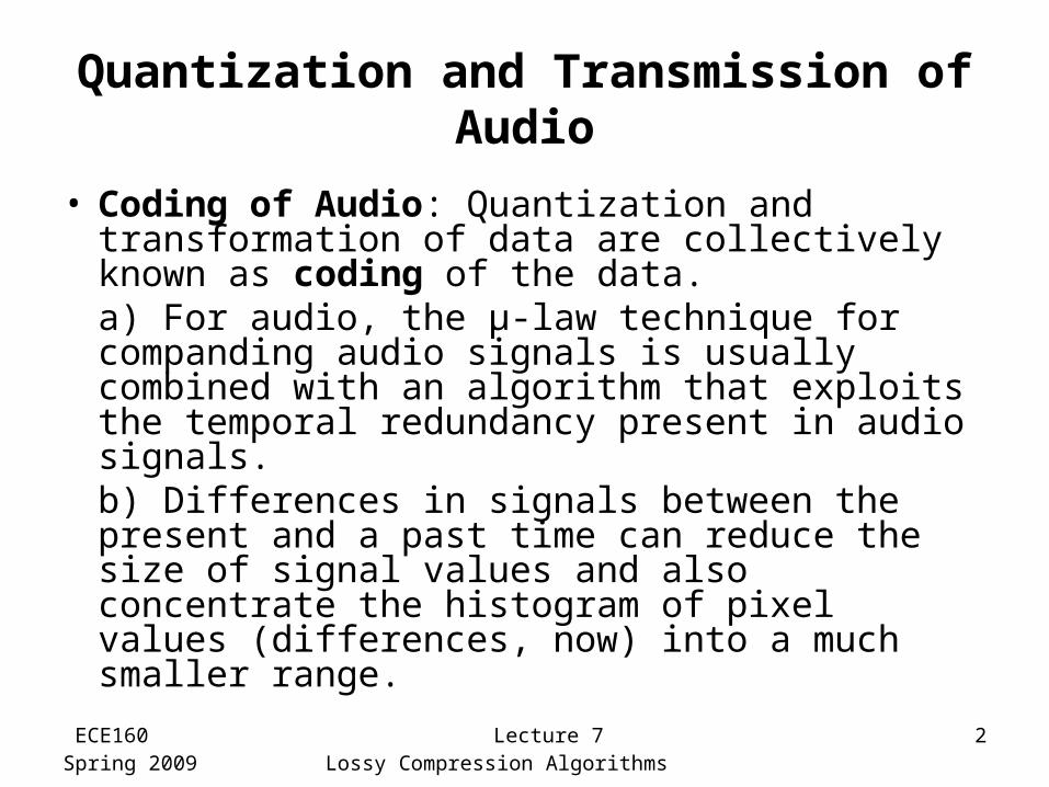
Quantization and Transmission of Audio

• Coding of Audio: Quantization and transformation of data are collectively known as coding of the data.a) For audio, the µ-law technique for companding audio signals is usually combined with an algorithm that exploits the temporal redundancy present in audio signals.b) Differences in signals between the present and a past time can reduce the size of signal values and also concentrate the histogram of pixel values (differences, now) into a much smaller range.

ECE160Spring 2009


3

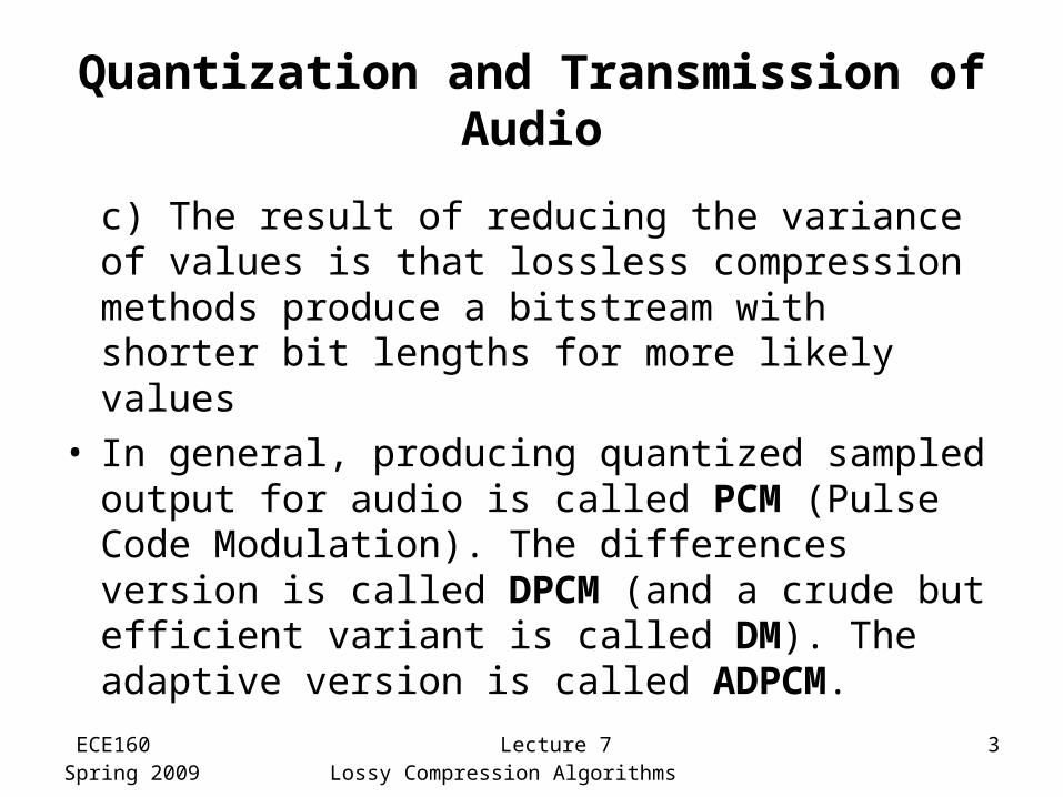
Quantization and Transmission of Audio

c) The result of reducing the variance of values is that lossless compression methods produce a bitstream with shorter bit lengths for more likely values

• In general, producing quantized sampled output for audio is called PCM (Pulse Code Modulation). The differences version is called DPCM (and a crude but efficient variant is called DM). The adaptive version is called ADPCM.

ECE160Spring 2009


4

Pulse Code Modulation

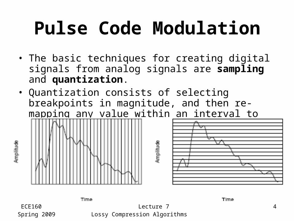
• The basic techniques for creating digital signals from analog signals are sampling and quantization.

• Quantization consists of selecting breakpoints in magnitude, and then re-mapping any value within an interval to one of the representative output levels.

ECE160Spring 2009


5


a) The set of interval boundaries are called decision boundaries, and the representative values are called reconstruction levels.b) The boundaries for quantizer input intervals that will all be mapped into the same output level form a coder mapping.c) The representative values that are the output values from a quantizer are a decoder mapping.

• d) Finally, we may wish to compress the data, by assigning a bit stream that uses fewer bits for the most prevalent signal values

ECE160Spring 2009


6


Every compression scheme has three stages:A. The input data is transformed to a new representation that is easier or more efficient to compress.B. We may introduce loss of information. Quantization is the main lossy step => we use a limited number of reconstruction levels, fewer than in the original signal.C. Coding. Assign a codeword (thus forming a binary bitstream) to each output level or symbol. This could be a fixed-length code, or a variable length code such as Huffman coding

ECE160Spring 2009


7

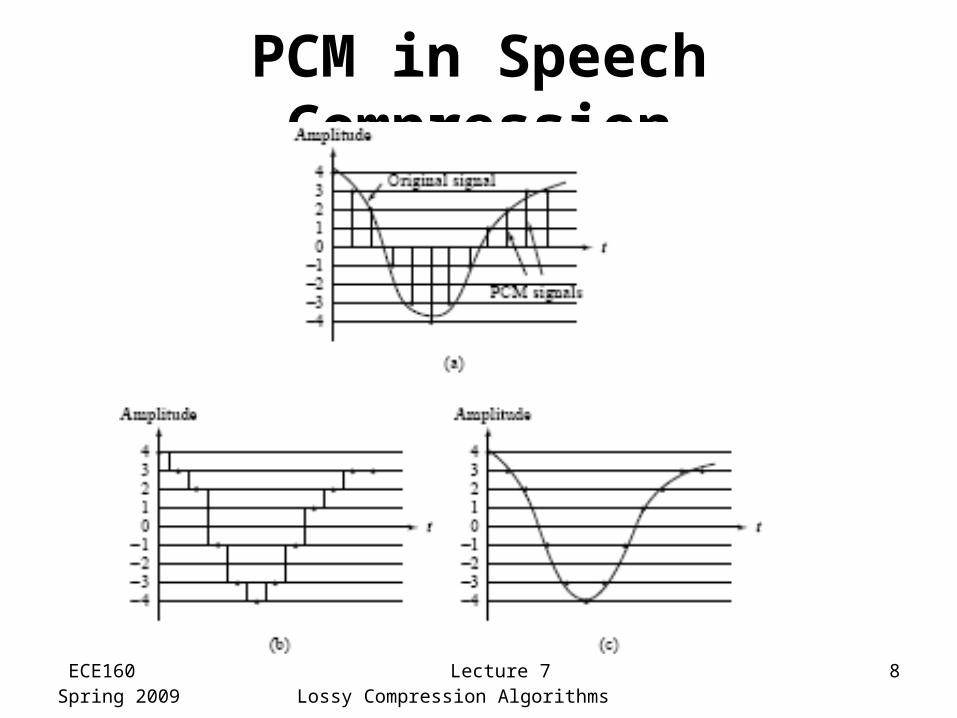
PCM in Speech CompressionAssuming a bandwidth for speech from about 50 Hz to about 10 kHz, the Nyquist rate would dictate a sampling rate of 20 kHz.

(a) Using uniform quantization without companding, the minimum sample size we could get away with would likely be about 12 bits. For mono speech transmission the bit-rate would be 240 kbps.(b) With companding, we can reduce the sample size down to about 8 bits with the same perceived level of quality, and thus reduce the bit-rate to 160 kbps.(c) However, the standard approach to telephony in fact assumes that the highest-frequency audio signal we want to reproduce is only about 4 kHz. Therefore the sampling rate is only 8 kHz, and the companded bit-rate thus reduces this to 64 kbps.(d) Since only sounds up to 4 kHz are to be considered, all other frequency content must be noise. Therefore, we remove this high-frequency content from the analog input signal using a band-limiting filter that blocks out high, as well as very low, frequencies.

ECE160Spring 2009


8

PCM in Speech Compression

ECE160Spring 2009


9

PCM in Speech Compression

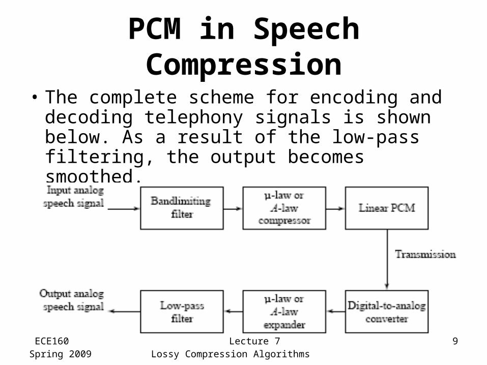
• The complete scheme for encoding and decoding telephony signals is shown below. As a result of the low-pass filtering, the output becomes smoothed.

ECE160Spring 2009


10

Differential Coding of Audio

• Audio is often stored in a form that exploits differences - which are generally smaller numbers, needing fewer bits to store them.(a) If a signal has some consistency over time (“temporal redundancy"), the difference signal, subtracting the current sample from the previous one, will have a more peaked histogram, with a maximum near zero.(b) For example, as an extreme case the histogram for a linear ramp signal that has constant slope is flat, whereas the histogram for the derivative of the signal (i.e., the differences from sampling point to sampling point) consists of a spike at the slope value.(c) If we assign codewords to differences, we can assign short codes to prevalent values and long codewords to rare ones.

ECE160Spring 2009


11

Lossless Predictive Coding

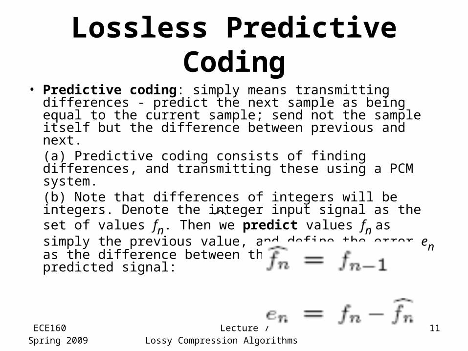
• Predictive coding: simply means transmitting differences - predict the next sample as being equal to the current sample; send not the sample itself but the difference between previous and next.(a) Predictive coding consists of finding differences, and transmitting these using a PCM system.(b) Note that differences of integers will be integers. Denote the integer input signal as the set of values fn. Then we predict values fn as simply the previous value, and define the error en as the difference between the actual and the predicted signal:

ECE160Spring 2009


12

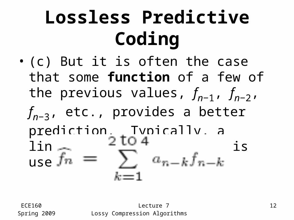
Lossless Predictive Coding

• (c) But it is often the case that some function of a few of the previous values, fn−1, fn−2, fn−3, etc., provides a better

prediction. Typically, a linear predictor function is used:

ECE160Spring 2009


13

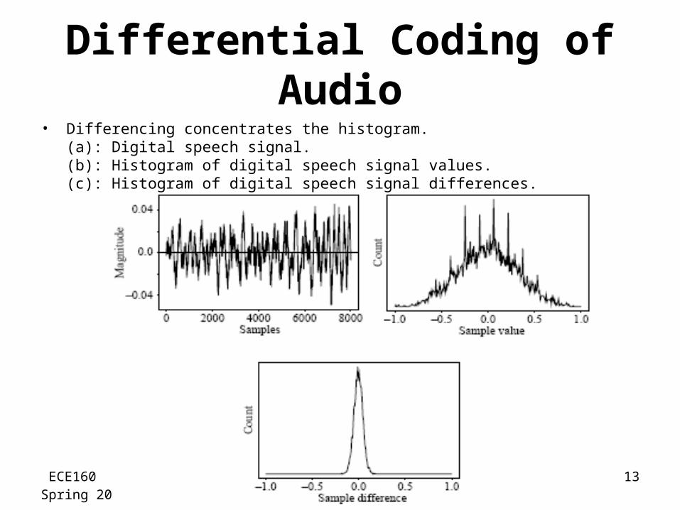
Differential Coding of Audio• Differencing concentrates the histogram.

(a): Digital speech signal. (b): Histogram of digital speech signal values.(c): Histogram of digital speech signal differences.

ECE160Spring 2009


14

Differential Coding of Audio

• One problem: suppose our integer sample values are in the range 0..255. Then differences could be as much as -255..255 - we've increased our dynamic range (ratio of maximum to minimum) by a factor of two and need more bits to transmit some differences.(a) A clever solution for this: define two new codes, denoted SU and SD, standing for Shift-Up and Shift-Down. Special code values are reserved for these.(b) We use codewords for only a limited set of signal differences, say only the range −15::16. Differences in the range are coded as is, a value outside the range −15::16 is transmitted as a series of shifts, followed by a value that is inside the range −15::16.(c) For example, 100 is transmitted as: SU, SU, SU, 4.

ECE160Spring 2009


18

DPCM

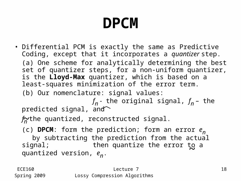
• Differential PCM is exactly the same as Predictive Coding, except that it incorporates a quantizer step.(a) One scheme for analytically determining the best set of quantizer steps, for a non-uniform quantizer, is the Lloyd-Max quantizer, which is based on a least-squares minimization of the error term.

(b) Our nomenclature: signal values: fn - the original signal, fn – the predicted signal, and

fn the quantized, reconstructed signal.

(c) DPCM: form the prediction; form an error en by subtracting the prediction from the actual signal; then quantize the error to a quantized version, en.

~

~

ECE160Spring 2009


19

DPCM

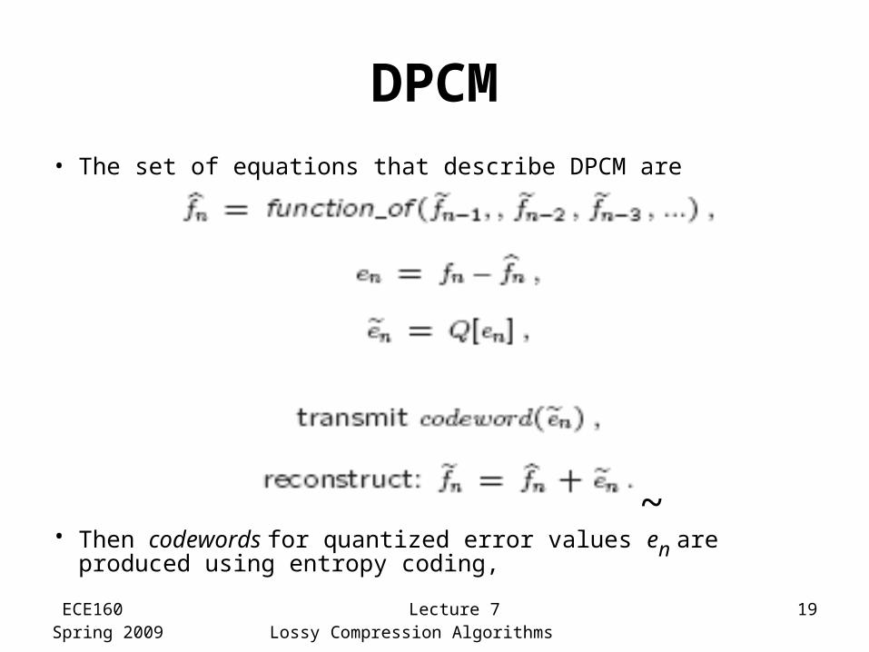
• The set of equations that describe DPCM are

• Then codewords for quantized error values en are produced using entropy coding,

~

ECE160Spring 2009


20

DPCM

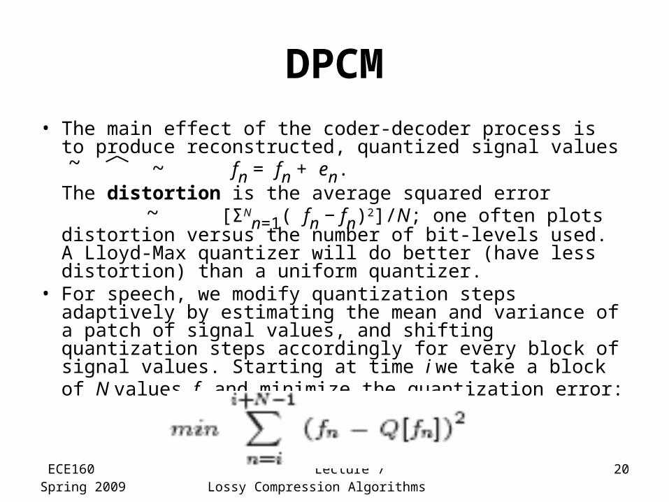
• The main effect of the coder-decoder process is to produce reconstructed, quantized signal values fn = fn + en.The distortion is the average squared error [ΣN

n=1( fn − fn)2]/N; one often plots distortion versus the number of bit-levels used. A Lloyd-Max quantizer will do better (have less distortion) than a uniform quantizer.

• For speech, we modify quantization steps adaptively by estimating the mean and variance of a patch of signal values, and shifting quantization steps accordingly for every block of signal values. Starting at time i we take a block of N values fn and minimize the quantization error:

~ ~

~

ECE160Spring 2009


21

DPCM

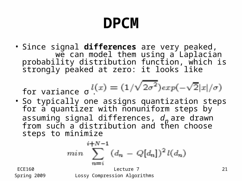
• Since signal differences are very peaked, we can model them using a Laplacian probability distribution function, which is strongly peaked at zero: it looks like

for variance σ2.• So typically one assigns quantization steps for a

quantizer with nonuniform steps by assuming signal differences, dn are drawn from such a distribution and then choose steps to minimize

ECE160Spring 2009


23

DM

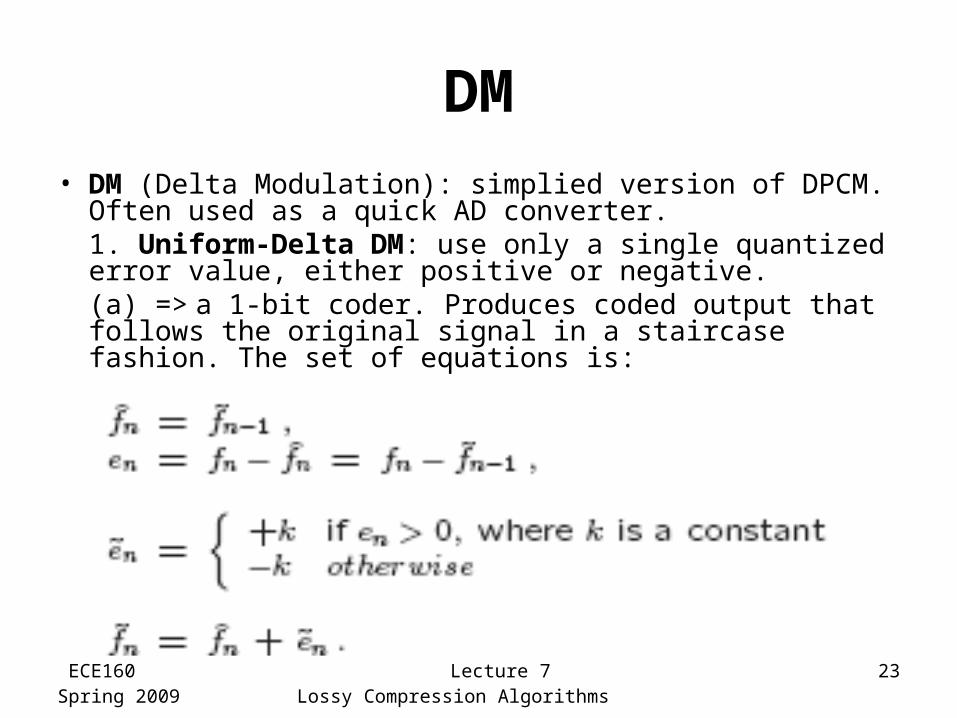
• DM (Delta Modulation): simplied version of DPCM. Often used as a quick AD converter.1. Uniform-Delta DM: use only a single quantized error value, either positive or negative.(a) => a 1-bit coder. Produces coded output that follows the original signal in a staircase fashion. The set of equations is:

ECE160Spring 2009


24

DM

• DM does not cope well with rapidly changing signals. One approach to mitigating this problem is to simply increase the sampling, perhaps to many times the Nyquist rate.

• Adaptive DM: If the slope of the actual signal curve is high, the staircase approximation cannot keep up. For a steep curve, can change the step size k adaptively.- One scheme for analytically determining the best set of quantizer steps, for a non-uniform quantizer, is Lloyd-Max.

ECE160Spring 2009


25

ADPCM

• ADPCM (Adaptive DPCM) takes the idea of adapting the coder to suit the input much farther. The two pieces that make up a DPCM coder: the quantizer and the predictor.1. In Adaptive DM, adapt the quantizer step size to suit the input. In DPCM, we can change the step size as well as decision boundaries, using a non-uniform quantizer.We can carry this out in two ways:(a) Forward adaptive quantization: use the properties of the input signal.(b) Backward adaptive quantizationor: use the properties of the quantized output. If quantized errors become too large, we should change the non-uniform quantizer.

ECE160Spring 2009


26

ADPCM

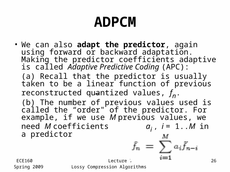
• We can also adapt the predictor, again using forward or backward adaptation. Making the predictor coefficients adaptive is called Adaptive Predictive Coding (APC):(a) Recall that the predictor is usually taken to be a linear function of previous reconstructed quantized values, fn.(b) The number of previous values used is called the “order" of the predictor. For example, if we use M previous values, we need M coefficients ai , i = 1..M in a predictor

~

ECE160Spring 2009


27

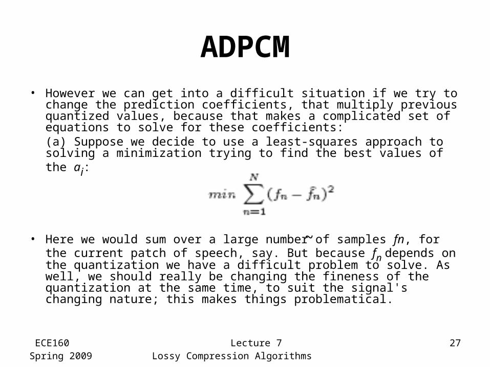
ADPCM• However we can get into a difficult situation if we try to change the

prediction coefficients, that multiply previous quantized values, because that makes a complicated set of equations to solve for these coefficients:(a) Suppose we decide to use a least-squares approach to solving a minimization trying to find the best values of the ai:

• Here we would sum over a large number of samples fn, for the current patch of speech, say. But because fn depends on the quantization we have a difficult problem to solve. As well, we should really be changing the fineness of the quantization at the same time, to suit the signal's changing nature; this makes things problematical.

~

ECE160Spring 2009


28

ADPCM

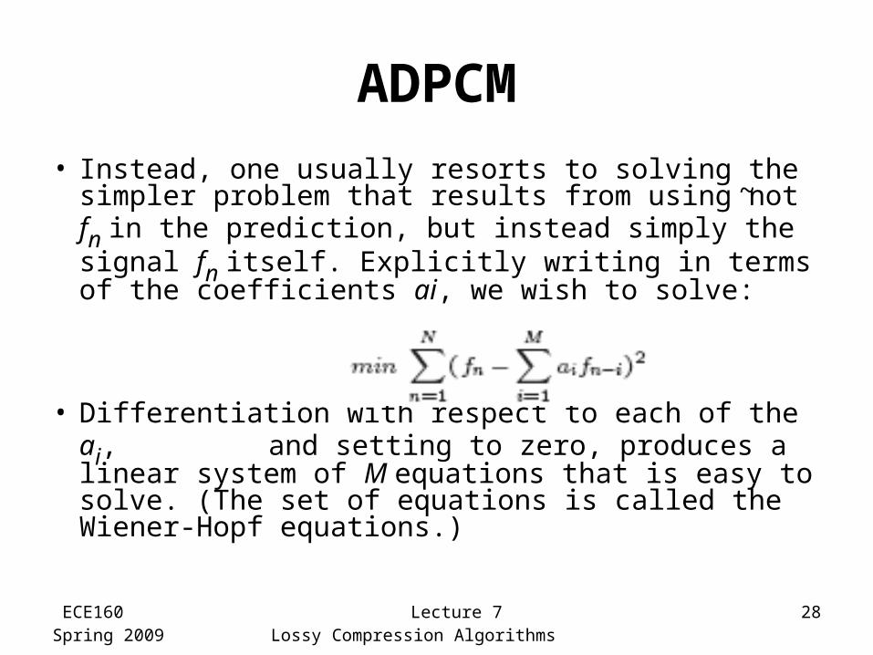
• Instead, one usually resorts to solving the simpler problem that results from using not fn in the prediction, but instead simply the signal fn itself. Explicitly writing in terms of the coefficients ai, we wish to solve:

• Differentiation with respect to each of the ai, and setting to zero, produces a linear system of M equations that is easy to solve. (The set of equations is called the Wiener-Hopf equations.)

~

ECE160Spring 2009


29

Dolby

• Dolby started by analog coding to hide hiss on cassette tapes. He amplified small sounds before recording and then reduced them (and the hiss) on playback.

• Dolby moved on to multichannel sound for movie widescreens (but no multichannels on the movie film).

• You will encounter Dolby AC-3, (5.1 channels), right front, center, left front, right rear, left rear and subwoofer. Dolby EX (6.1) has a center rear Dolby TrueHD has 8 channels and high quality

ECE160Spring 2009


30

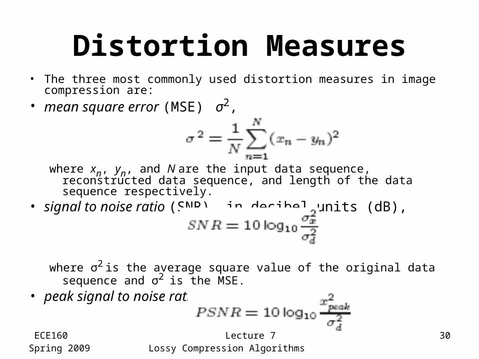
Distortion Measures• The three most commonly used distortion measures in image

compression are:

• mean square error (MSE) σ2,

where xn, yn, and N are the input data sequence, reconstructed data sequence, and length of the data sequence respectively.

• signal to noise ratio (SNR), in decibel units (dB),

where σ2 is the average square value of the original data sequence and σ2 is the MSE.

• peak signal to noise ratio (PSNR),

ECE160Spring 2009


31

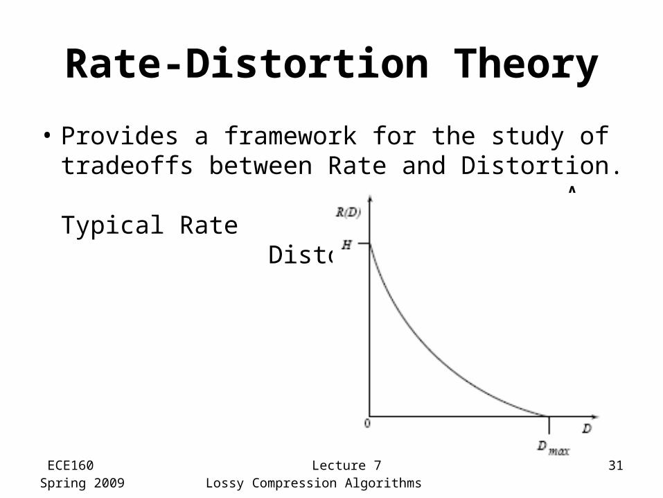
Rate-Distortion Theory

• Provides a framework for the study of tradeoffs between Rate and Distortion. A Typical Rate Distortion Function:

ECE160Spring 2009


32

Quantization

• Reduce the number of distinct output values to a much smaller set.

• Main source of the “loss" in lossy compression.

• Three different forms of quantization.– Uniform: midrise and midtread quantizers.– Nonuniform: companded quantizer.– Vector Quantization.

ECE160Spring 2009


33

Uniform Scalar Quantization

• A uniform scalar quantizer partitions the domain of input values into equally spaced intervals, except possibly at the two outer intervals.– The output or reconstruction value corresponding to

each interval is taken to be the midpoint of the interval.

– The length of each interval is referred to as the step size, denoted by the symbol Δ.

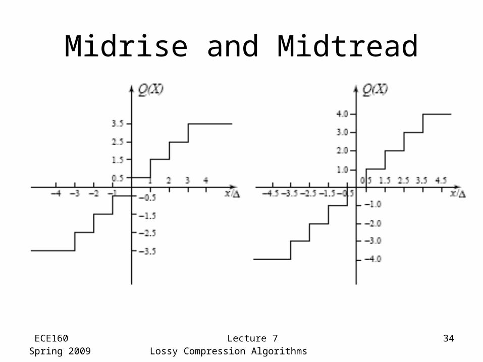
• Two types of uniform scalar quantizers:– Midrise quantizers have even number of output levels.– Midtread quantizers have odd number of output

levels, including zero as one of them

ECE160Spring 2009


34

Midrise and Midtread

ECE160Spring 2009


35

Uniform Scalar Quantization

• For the special case where Δ = 1, we can simply compute the output values for these quantizers as:

Qmidrise(x) = x − 0:5

Qmidtread(x) = x+0:5• Performance of an M level quantizer.

Let B = {b0, b1,…,bM} be the set of decision boundaries and Y = {y1, y2,…, yM} be the set of reconstruction or output values.

• Suppose the input is uniformly distributed in the interval [−Xmax,Xmax]. The rate of the quantizer is:

R = log2M

ECE160Spring 2009


36

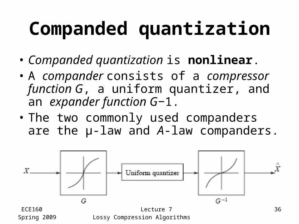
Companded quantization

• Companded quantization is nonlinear.• A compander consists of a compressor

function G, a uniform quantizer, and an expander function G−1.

• The two commonly used companders are the µ-law and A-law companders.