


Languages
Pages
Legal


Strain analysis [email protected]
Plates vs. continuum
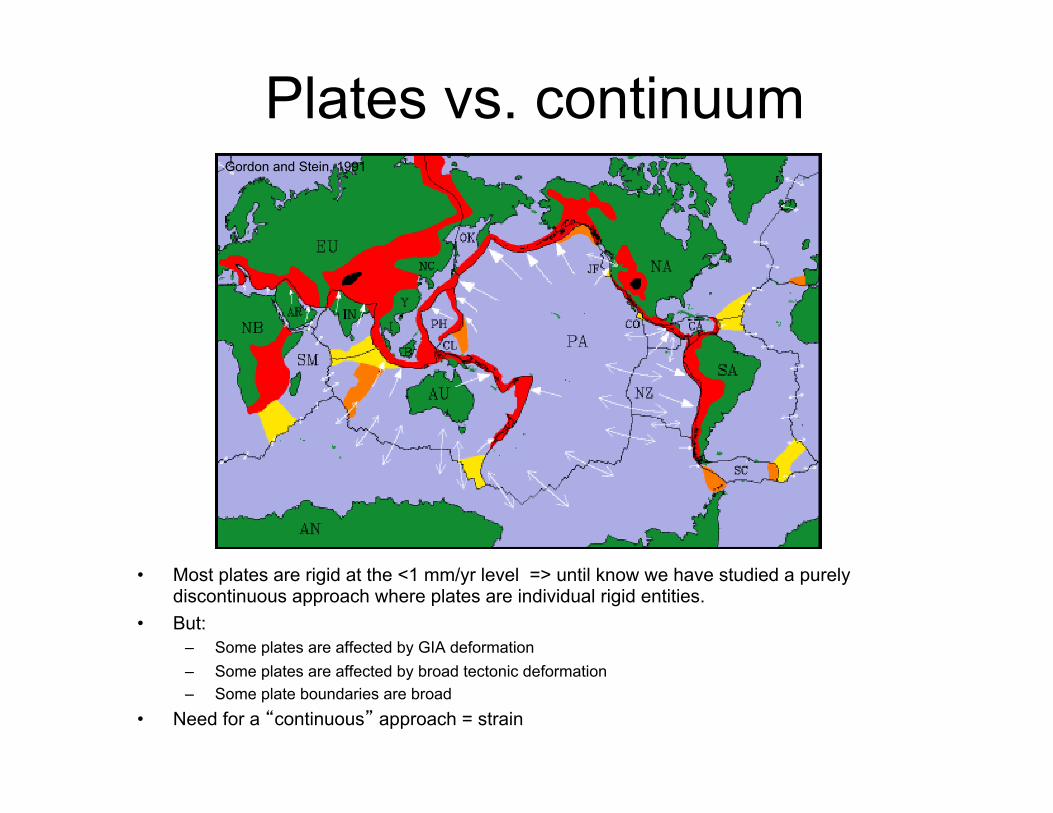
• Most plates are rigid at the <1 mm/yr level => until know we have studied a purely discontinuous approach where plates are individual rigid entities.
• But: – Some plates are affected by GIA deformation – Some plates are affected by broad tectonic deformation – Some plate boundaries are broad
• Need for a “continuous” approach = strain
Gordon and Stein, 1991
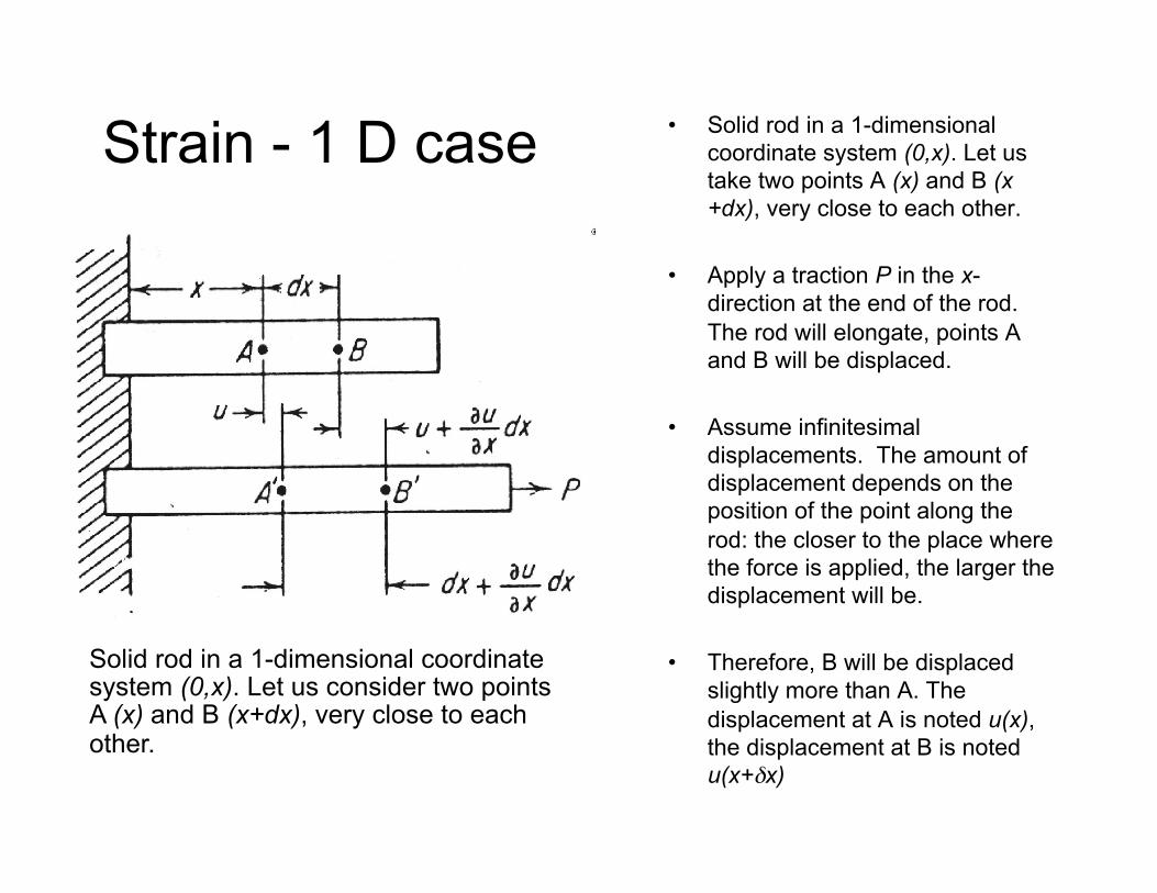
Strain - 1 D case • Solid rod in a 1-dimensional coordinate system (0,x). Let us take two points A (x) and B (x+dx), very close to each other.
• Apply a traction P in the x-direction at the end of the rod. The rod will elongate, points A and B will be displaced.
• Assume infinitesimal displacements. The amount of displacement depends on the position of the point along the rod: the closer to the place where the force is applied, the larger the displacement will be.
• Therefore, B will be displaced slightly more than A. The displacement at A is noted u(x), the displacement at B is noted u(x+δx)
Solid rod in a 1-dimensional coordinate system (0,x). Let us consider two points A (x) and B (x+dx), very close to each other.
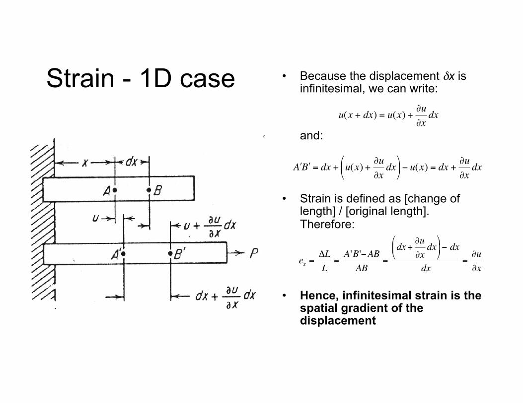
Strain - 1D case • Because the displacement δx is infinitesimal, we can write:
and:
• Strain is defined as [change of length] / [original length]. Therefore:
• Hence, infinitesimal strain is the spatial gradient of the displacement
€
u(x + dx) = u(x) +∂u∂xdx
€
ex =ΔLL
=A 'B'−ABAB
=dx+
∂u∂xdx
%
& '
(
) * − dx
dx=∂u∂x
€
" A " B = dx + u(x) +∂u∂x
dx$
% &
'
( ) − u(x) = dx +
∂u∂x
dx

2D case: velocity gradient tensor • Assuming:
– Local 2-dimensional Cartesian frame – Infinitesimal displacements
• Velocity (as a function of position X) can be expanded in a series:
• With the two components:
• Therefore, one can write:
€
v(X + δX) = v(X) +∂v∂X
δX
€
vx (X + δX) = vx (X) +∂vx∂x
δx +∂vx∂y
δy
vy (X + δX) = vy (X) +∂vy∂x
δx +∂vy∂y
δy
$
% & &
' & &
€
v(X + δX) = v(X) +∇V .δX
€
∇V =
∂vx∂x
∂vx∂y
∂vy∂x
∂vy∂y
$
%
& & & &
'
(
) ) ) )
with = velocity gradient tensor
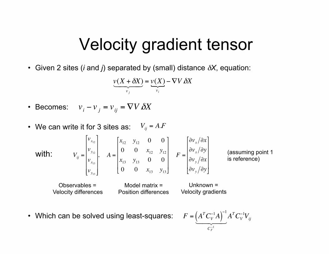
Velocity gradient tensor • Given 2 sites (i and j) separated by (small) distance δX, equation:
• Becomes:
• We can write it for 3 sites as:
• Which can be solved using least-squares:
€
v(X + δX)v j
= v(X)vi −∇V .δX
€
vi − v j = vij =∇V .δX
€
Vij =
vx12vy12vx13vy13
"
#
$ $ $ $ $
%
&
' ' ' ' '
, A =
x12 y12 0 00 0 x12 y12x13 y13 0 00 0 x13 y13
"
#
$ $ $ $
%
&
' ' ' '
F =
∂vx ∂x∂vx ∂y∂vy ∂x∂vy ∂y
"
#
$ $ $ $
%
&
' ' ' '
€
Vij = A.F
Observables = Velocity differences
Model matrix = Position differences
(assuming point 1 is reference)
with:
Unknown = Velocity gradients
€
F = ATCV−1A( )
−1
CF−1
ATCV
−1Vij

Velocity gradient tensor: covariance
• Observables are velocity differences.The covariance associated with vij can then be found using:
• One usually knows the covariance matrix Cind of the individual site velocities -- the variance propagation law then gives:
• CVij is then propagated in the least squares estimation (see previous slide) to get the covariance matrix of the unknowns CF. €
CVij= A.Cind .A
T
€
vxijvyij
"
# $
%
& ' =
−1 0 1 00 −1 0 1"
# $
%
& '
A
vxivyivxjvyi
"
#
$ $ $ $
%
&
' ' ' '

Velocity gradient tensor: covariance of unknowns
• Given that:
• One can write the variance on the east (for instance) component of the velocity difference as:
• Therefore, if the covariance terms are large enough, velocities can be non-significant while relative velocities (and velocity gradient tensor) are… €
σ eij2 =σ ei
2 +σ e j2 − 2σ ei e j
€
CVij= A.Cind .A
T

Strain and rotation rates • Displacements actually combine strain and a rigid-body rotation. • Tensor theory states that any second-rank tensor can be
decomposed into a symmetric and an antisymmetric tensor. One can therefore write:
€
∇V =12∇V +∇VT[ ] +
12∇V −∇VT[ ]
⇔∇V =
∂vx∂x
12∂vx∂y
+∂vy∂x
&
' (
)
* +
12∂vx∂y
+∂vy∂x
&
' (
)
* +
∂vy∂y
,
-
.
.
.
.
/
0
1 1 1 1
+0 1
2∂vx∂y
−∂vy∂x
&
' (
)
* +
12∂vy∂x
−∂vx∂y
&
' (
)
* + 0
,
-
.
.
.
.
/
0
1 1 1 1
Symmetric tensor Antisymmetric tensor
Strain and rotation rates
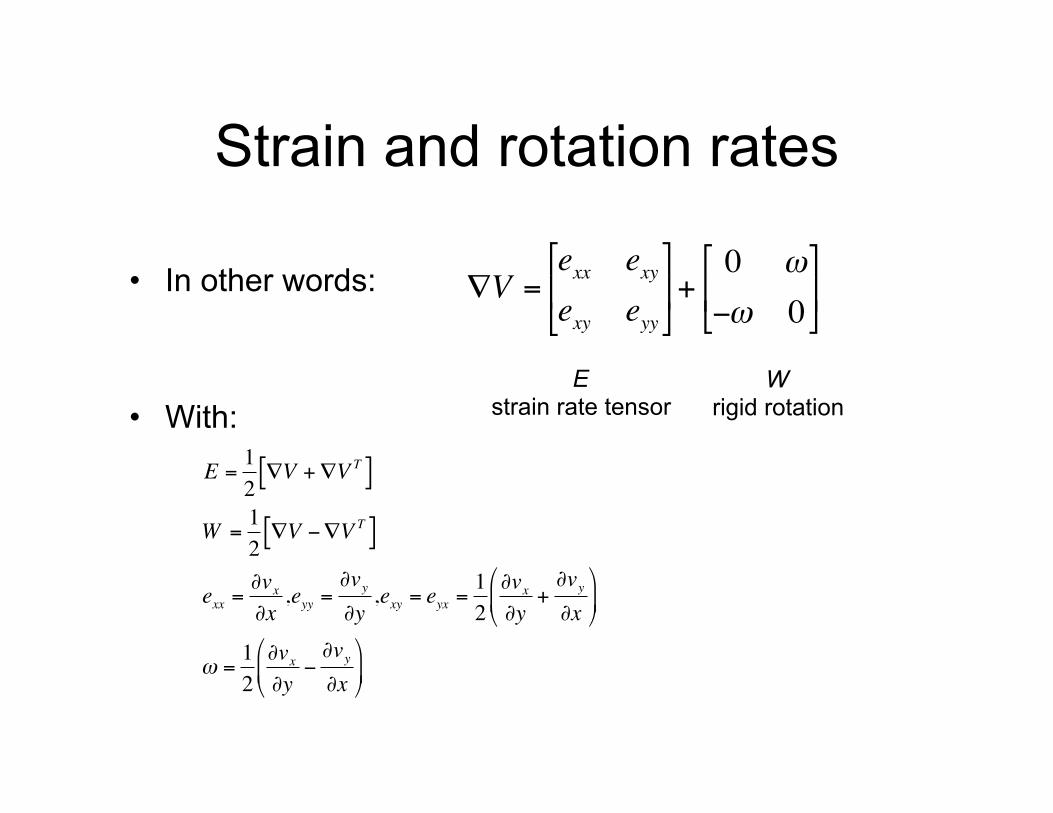
• In other words:
• With: €
∇V =exx exyexy eyy
#
$ %
&
' ( +
0 ω
−ω 0#
$ %
&
' (
E strain rate tensor
W rigid rotation
€
E =12∇V +∇VT[ ]
W =12∇V −∇VT[ ]
exx =∂vx∂x,eyy =
∂vy∂y,exy = eyx =
12∂vx∂y
+∂vy∂x
%
& '
(
) *
ω =12∂vx∂y
−∂vy∂x
%
& '
(
) *

Estimating strain rate • Given 2 sites (i and j), one can write the velocity difference (w.r.t. site i) as a function of the
site position (w.r.t. site I) as:
• For 3 sites as, this can be written as:
with:
• Which can be solved using least-squares:
€
vij =∇V .δX⇔ vij = (E +W ).δX
⇔vxij = exxδx + exyδy +ωδyvyij = exyδx + eyyδy −ωδx' ( )
€
Vij =
vx12vy12vx13vy13
"
#
$ $ $ $ $
%
&
' ' ' ' '
, A =
x12 y12 0 y120 x12 y12 −x12x13 y13 0 y130 y13 y13 −x13
"
#
$ $ $ $
%
&
' ' ' '
S =
exxexyeyyω
"
#
$ $ $ $
%
&
' ' ' '
€
Vij = A.S
Observables = velocity differences
Model matrix = Position differences
€
S = ATCV−1A( )
−1
CS−1
ATCV
−1Vij

Estimating strain: A better approach
• First, estimate velocity gradient components (and covariance) using least squares (see previous slides).
• Then, recall that:
• Therefore, strain and rotation rate components can be found using the following transformation matrix:
• Propagate velocity gradient covariance to strain and rotation rate covariance using:
€
exx =∂vx∂x,eyy =
∂vy∂y,exy = eyx =
12∂vx∂y
+∂vy∂x
#
$ %
&
' ( ,ω =
12∂vx∂y
−∂vy∂x
#
$ %
&
' (
€
exxexyeyyω
#
$
% % % %
&
'
( ( ( (
=
1 0 0 00 0.5 0.5 00 0 0 10 0.5 −0.5 0
*
+
, , , ,
-
.
/ / / /
A
∂vx∂x∂vx∂y∂vy∂x∂vy∂y
#
$
% % % % % % % %
&
'
( ( ( ( ( ( ( (
€
CE ,W = AC∇V AT

Representing strain • Tensor = independent of
the coordinate system = retains its properties independently from the ref. system.
• Find reference system where: – Shear strain (exy) is zero – Two other components are
maximal • Equivalent to diagonalize E:
– Eigenvectors = principal axes of strain rate tensor
– Eigenvalues = principal strain rates

Principal strains
• Principal values of E: (= principal strains)
• Principal directions: – Use rotation matrix A: – Expand AEAT and write that shear component = 0 to find:
€
det(E − λI) = 0
⇒ detexx − λ exyexy eyy − λ
%
& '
(
) * = 0
⇒ exx − λ( ) eyy − λ( ) − exyexy = 0
⇒ λ =exx + eyy2
±exx − eyy2
+
, -
.
/ 0
2
+ exy2
€
e12 = (exx − eyy )sinθ cosθ + exy (cos2θ − sin2θ) = 0
⇒ tan(2θ) =2exy
exx − eyy
€
A =cosθ −sinθsinθ cosθ$
% &
'
( )
€
sinθ cosθ =12sin 2θ( )
cos2θ − sin2θ = cos 2θ( )

Principal strains
• Principal strains: – One maximal, one minimal – By convention, extension is
taken positive
• Principal angle (direction of e1):
€
e1,e2 =exx + eyy2
±exx − eyy2
#
$ %
&
' (
2
+ exy2
€
tan(2θ) =2exy
exx − eyy

Back transformation • Rotate principal strain rate tensor by angle -θ using rotation matrix A:
• Recall that tensor rotation is given by:
• Which gives:
€
exx = e1 cos2θ + e2 sin
2θ =e1 + e22
+e1 − e22
cos 2θ( )
eyy = e1 sin2θ + e2 cos
2θ =e1 + e22
−e1 − e22
cos 2θ( )
exy = −e1 sinθ cosθ + e2 sinθ cosθ = −e1 − e22
sin 2θ( )
$
%
& &
'
& &
€
sinθ cosθ =12sin 2θ( )
cos2θ − sin2θ = cos 2θ( )
€
A =cosθ sinθ−sinθ cosθ$
% &
'
( )
€
AEpAT =
e1 cos2θ + e2 sin
2θ −e1 sinθ cosθ + e2 sinθ cosθ−e1 sinθ cosθ + e2 sinθ cosθ e1 sin
2θ + e2 cos2θ
$
% &
'
( )

• Shear strain (from previous transformation) is maximal when sin(2θ)=1, giving:
• Recall the expression for e12 (which we set to zero to find the principal angle θ):
• Angle at which shear strain is maximal is obtained by differentiating w.r.t. θ:
Shear strain
€
exy = −e1 − e22
sin 2θ( )
⇒ exy,max =e1 − e22
=exx − eyy2
%
& '
(
) *
2
+ exy2
€
e12 = (exx − eyy )sinθ cosθ + exy (cos2θ − sin2θ)
=12(exx − eyy )sin 2θ( ) + exy cos 2θ( )
€
e12 =max⇒ de12dθ
= 0
12(eyy − exx )cos 2θS( ) − exy sin 2θS( ) = 0
⇒ tan 2θS( ) =eyy − exx2exy
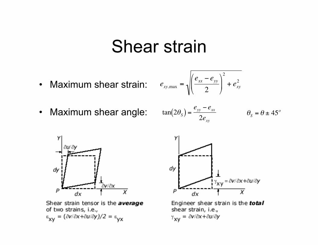
Shear strain
• Maximum shear strain:
• Maximum shear angle: €
exy,max =exx − eyy2
#
$ %
&
' (
2
+ exy2
€
tan 2θS( ) =eyy − exx2exy
€
θS = θ ± 45o

Example 1: pure extension • Strain rate tensor:
– exx = 0.00 ppb/yr – exy = -0.00 ppb/yr – eyy = 177.08 ppb/yr
• Principal strains: – e1 = 177.08 ppb/yr (most
extensional) – e2 = 0.00 ppb/yr (most
compressional) – theta = 90.00 (e1, CW from
north) • Rotation:
– omega = 0.00 deg/My

Example 2: simple shear
• Strain rate tensor: – exx = 0.00 ppb/yr – exy = 88.54 ppb/yr – eyy = -0.00 ppb/yr
• Principal strains: – e1 = 88.54 ppb/yr (most
extensional) – e2 = -88.54 ppb/yr (most
compressional) – theta = -45.00 (e1, CW
from north) • Rotation:
– omega = 0.09 deg/My
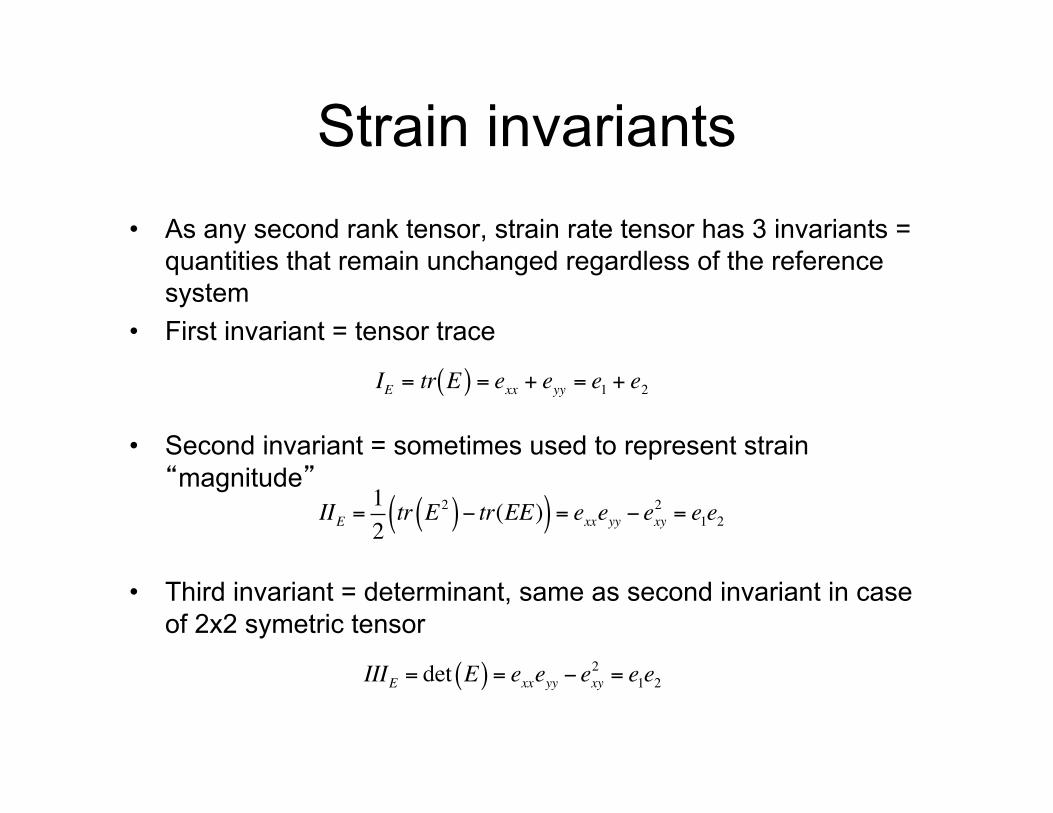
• As any second rank tensor, strain rate tensor has 3 invariants = quantities that remain unchanged regardless of the reference system
• First invariant = tensor trace
• Second invariant = sometimes used to represent strain “magnitude”
• Third invariant = determinant, same as second invariant in case of 2x2 symetric tensor
Strain invariants
€
IE = tr E( ) = exx + eyy = e1 + e2
IIE =12tr E 2( )− tr(EE)( ) = exxeyy − exy2 = e1e2
IIIE = det E( ) = exxeyy − exy2 = e1e2

Example: current strain rates in Asia
• The 3x10⁻⁹ yr-1 line coincides with the 95% significance level • A large part of Asia shows strain rates that are not significant at the 95% confidence level
and are lower than 3x10⁻⁹ yr-1

In practice • Discretize space • Using polygons with vertices
corresponding to data points • For instance: Delaunay
triangulation: – Circumcircle of every triangle
does not contain any other point of the triangulation
– Minimize “sliver” triangles • Using arbitrary polygons:
requires interpolation • Calculate strain within each
polygon
WARNING: assumes homogeneous and
continuous strain within each polygon…
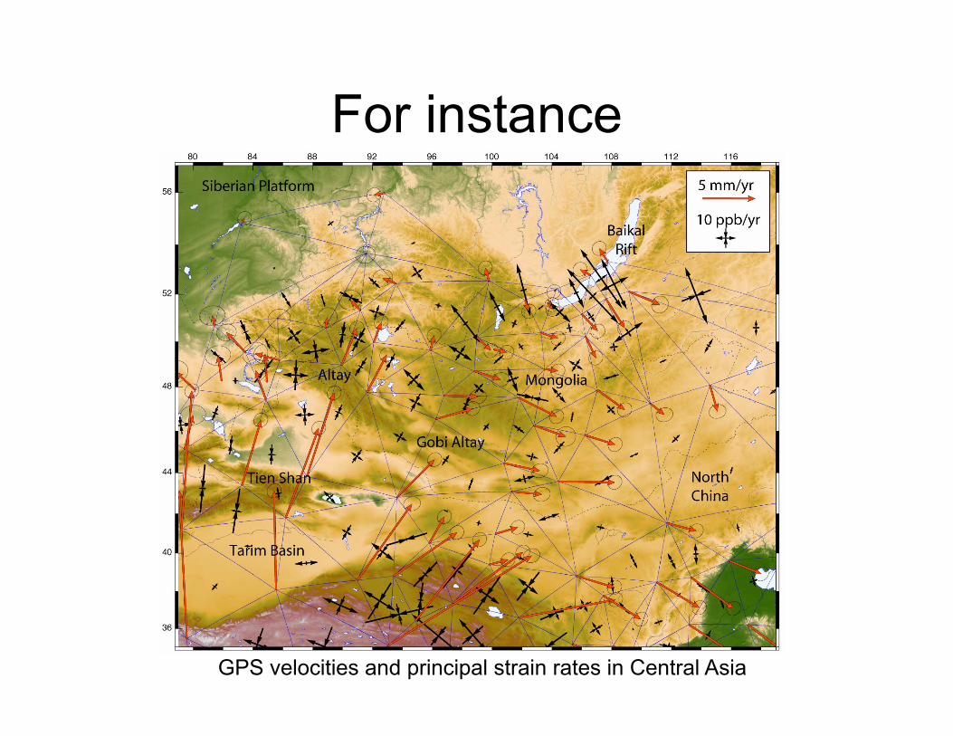
For instance
GPS velocities and principal strain rates in Central Asia

WARNING! • Result depends on the size
of the elements used to discretize the domain…
• Example: – Generate a random 2D
velocity field (e.g. case of non significant residual velocities showing only noise)
– Triangulate with smaller elements in the middle of the domain
– Calculate strain – Result will be apparently
larger strain rates where elements are smaller…
Top Related