


Languages
Pages
Legal


Dynamic Price Competition, Learning-By-Doing andStrategic Buyers
Andrew Sweeting
UMD and NBER*
Dun Jia
Renmin University
Shen Hui
CUHK at Shenzhen
Xinlu Yao
UMD
August 29, 2020
Abstract
We generalize recent models of dynamic price competition where sellers benefit from learning-
by-doing to allow for forward-looking strategic buyers, with a single parameter capturing the
extent to which each buyer internalizes future buyer surplus. We show how that even moderate
strategic behavior can eliminate many of the equilibria that exist when buyers are atomistic or
myopic. When equilibria are eliminated, the ones that survive tend to be those where long-run
market competition is preserved. The results are relevant for both antitrust policy and the
future modeling of industries where learning-by-doing is important.
*Corresponding author: [email protected]. Andrew Sweeting is currently serving as Director of the Bureau ofEconomics at the Federal Trade Commission (FTC). The views expressed are those of the authors, and do not reflectthe views of the FTC, its staff or any individual Commissioner. We are very grateful to Uli Doraszelski and SteveKryukov for access to their computational results which helped to confirm our own results with non-strategic buyers.We are also grateful for comments received from conference and seminar participants at Penn State, the FTC andthe Washington DC IO conference. All errors are our own, and comments are very welcome.
1

1 Introduction
In industries where firms benefit from learning-by-doing (LBD), there is a natural tension between
achieving productive efficiency, which will require concentrating production at a single producer, and
sustaining competition, which may require spreading production across multiple firms. Economists
have analyzed a range of models to understand whether unregulated market equilibria will sustain
competition, how efficient these equilibria are and how surplus is split between customers and
producers.
One literature has used analytical theory to consider models where there are two competing
suppliers and single long-lived buyer who purchases a single unit each period and cannot commit
to long-run contracts (Lewis and Yildirim (2002)).1 The Lewis and Yildirim model has a unique
Markov Perfect equilibrium where the monopsonist spreads its purchases across duopolists to main-
tain competition, although this strategy can raise prices as sellers have weaker incentives to gain
an advantage.
A second literature also assumes that there is a buyer who purchases a single unit each period,
but makes the assumption that these buyers are atomistic in the sense that they are only in the
market once (i.e., that they are short-lived) or, equivalently, that they make their purchase deci-
sions myopically. Most notably, Cabral and Riordan (1994) consider a model where duopolists sell
differentiated products, cost reductions stop once a certain level of cumulative sales is reached and
there is an infinite sequence of short-lived buyers with heterogeneous preferences over the sellers.
They show that when a supplier may choose to exit, equilibria where firms price aggressively to try
to drive their rival out of the market can exist, and markets can tend towards monopoly.
This observation has led David Besanko and co-authors to use computational methods to ana-
lyze, in a systematic way, Markov Perfect equilibrium behavior in enriched versions of the Cabral
and Riordan model, while maintaining the assumption of short-lived buyers. Besanko, Doraszelski,
and Kryukov (2014) (BDK1) and Besanko, Doraszelski, and Kryukov (2019a) (BDK2) both use
a model, which we will refer to as the “BDK model”, that allows for the possibility of firm exit.
They quantify, for a range of parameter values, the incentives of sellers to “predate”, the effects of
different rules that prevent sellers from acting on predatory incentives, and distortions from first-
1Lewis and Yildirim (2005) and Anton, Biglaiser, and Vettas (2014) provide related models where a monopsoniststrategic buyer seeks to maintain competition between duopolist suppliers. Saini (2012) shows similar qualitativeeffects in a computational model of repeated procurement.
2

best outcomes across equilibria.2 They show that equilibria where one firm is likely to emerge as
dominant often co-exist with equilibria where competition is certain to be sustained in the long-run.
Besanko, Doraszelski, Kryukov, and Satterthwaite (2010) (BDKS) show that one can also generate
multiple equilibria, in some of which a single firm may end up achieving a dominant position, in a
model where exit is not possible but a firm’s experience stochastically decays (“forgetting”). For-
getting has been identified empirically in industries with LBD by Benkard (2000) amongst others.
The explanation is that, just like in a model where a rival may exit, forgetting creates the possibility
that a firm can cause its rival to move up its cost curve if it sets a very low price to deprive that
rival of sales.
However, neither the atomistic nor the monopsony buyer frameworks apply neatly to most in-
dustries where LBD has been documented, such as aircraft manufacture (Alchian (1963), Benkard
(2000)), power plants (Zimmerman (1982)), shipbuilding (Thompson (2001), Thornton and Thomp-
son (2001)), semiconductors (Irwin and Klenow (1994), Dick (1991)) and chemicals (Lieberman
(1984), Lieberman (1987)) as these industries have a non-trivial proportion of large and repeat
customers.3 For example, for civilian aircraft, a small number of carriers often account for a signif-
icant share of the orders for particular models and it is common for the world’s largest carriers and
aircraft leasing companies to buy significant numbers of similar types of planes sold by different
manufacturers.4
In this paper we therefore study what happens to equilibrium behavior and outcomes when
buyers are forward-looking and strategic, in the sense that they take some account of how their
choices affect future buyer surplus, without assuming that they do so completely (i.e., we consider
cases between atomistic buyers and monopsony). We do so by extending the BDK and BDKS
models using one additional parameter to capture how much of its effect on future surplus a buyer
internalizes, and we examine what happens to the multiplicity of equilibria, long-run competition
and welfare as this parameter is varied.
2Besanko, Doraszelski, and Kryukov (2019b) look in more detail at the implementation of different predationtests within these models.
3Even in the case of hospital procedures (Gaynor, Seider, and Vogt (2005), Dafny (2005)) where an individualpatient may hope to only purchase the service once, their choices are influenced by physician groups and payers thatknow they will be dealing with similar patients in the future.
4For example, by July 2020 242 Airbus A380s have been delivered to 14 different buyers, with a buyer-sideHHI (based on the number of aircraft sold to different airlines) of 0.239 (source, accessed July 18, 2020: https:
//en.wikipedia.org/wiki/List_of_Airbus_A380_orders_and_deliveries). Details on fleets by carrier in May2019 reported by Air Transport World (July/August 2019 edition, pages 45-55, accessed August 16, 2020). Forexample, Delta’s fleet included 213 Boeing 737s and 62 Airbus A320s. Of course, some carriers, such as Southwestare known to purchase planes from a single manufacturer (in this case, Boeing).
3

We have several substantive findings. As buyers become more strategic, equilibrium multiplicity
tends to be eliminated, a result that is interesting given that Besanko et al. find that, with atomistic
buyers, multiplicity is the “norm rather than the exception” (BDK1, p. 888) in these models. For
parameters for which, with atomistic buyers, equilibria that can give rise to long-run dominance
coexist with equilibria that always result in long-run competition, it is the equilibria with long-run
competition that tend to survive as buyers become strategic. As a result, strategic buyers tend to
lower expected long-run prices, although, when both firms start at the top of their learning curves,
the net present value (NPV) of buyer welfare can be reduced when buyers act strategically as the
initial competition between sellers to gain an advantage is softened. While these qualitative results
might be expected given what we know happens under monopsony, a striking finding is that the
multiplicity of equilibria can be eliminated even when buyers only internalize a small proportion
of their effects on future buyer surplus, which, in our framework, can be viewed as equivalent
to the buyer-side of the market being relatively unconcentrated. We find that the elimination of
multiplicity with relatively limited strategic behavior by buyers is particularly the case in the BDKS
model.
Our results have implications for both antitrust policy and the future modeling of industries
where firms can benefit from LBD. The existence of equilibria where a single firm can establish
dominance through aggressive pricing that leads a rival to exit suggests that claims of “predatory
pricing” may be plausible. Even though claims of predation are often hard to evaluate, the coexis-
tence of these types of equilibria with ones where long-run competition is maintained suggests that
an active anti-predation enforcement policy could be needed to push industries towards more com-
petitive outcomes in the long-run. BDK1 illustrate this result by showing that aggressive equilibria
tend to be eliminated when, in a counterfactual world, firms are not allowed to consider certain
predatory incentives when choosing prices.5 Our results, while generated from a specific model, sug-
gest that even quite moderate buyer-side concentration, a common real-world phenomenon, may
have similar effects, and make it appropriate to treat claims of predatory pricing more skeptically
in markets where repeat buyers are even moderately important.6
In terms of modeling our paper contributes to the emerging literatures in both economics and
5As BDK1 and BDK2 point out, demand-side network effects may create similar economic incentives to learning-by-doing so that one would expect that predation could also be an equilibrium outcome in network effect marketswith suitable parameters.
6Of course, if we added features, such as financial constraints or asymmetric information, that are not featuresof the Cabral and Riordan (1994), BDKS or BDK models, or the models considered here, it may be that predatoryequilibria could re-emerge. This is an important topic for future research.
4

management science that consider how larger and more sophisticated buyers can affect how mar-
kets work (for example, Jerath, Netessine, and Veeraraghavan (2010), Horner and Samuelson (2011),
Board and Skrzypacz (2016), Chen, Farias, and Trichakis (2019) and, motivated by antitrust analy-
sis, Loertscher and Marx (2019)). In particular, we show how even limited strategic buyer behavior
affects outcomes in an infinite horizon model that has quite rich supply-side competitive dynamics.
Our results also suggest that empirical analyses of industries with LBD where atomistic buyers
have been assumed for convenience (for example, Benkard (2004), Kim (2014)) could give different
results if strategic buyer behavior was accounted for. More encouragingly, however, our results also
suggest that allowing for strategic buyer behavior may not only add realism to empirical analyses,
but also reduce concerns that the possibility of multiple equilibria, which is often hard to detect,
may undermine the researcher’s ability to interpret structural counterfactuals.
In this regard, we make one methodological contribution that is also potentially helpful. The
Besanko et al. papers enumerate equilibria using homotopy techniques that follow equilibrium
correspondences. However, the homotopy approach is not guaranteed to find all equilibria, so
claims of uniqueness, like the ones that we would like to make, based on homotopy results may not
be convincing. In our analysis of the extended BDK model, we therefore also consider an alternative
method of proof that allows us to make statements about the existence and non-existence particular
types of equilibria. Specifically, we use backwards induction methods that can prove the existence
or non-existence of either equilibria where firms never exit, which we find must always be unique, or
equilibria where exit from at least some states will result in permanent monopoly. These two groups
turn out to include all of the equilibria that homotopies identify for the parameters we consider in
this paper where learning-by-doing is present. Therefore, when we prove that no equilibria of the
second type exist, we have additional evidence that an equilibrium with no exit is unique. As we
find that our results using this alternative approach are consistent with those using homotopies,
this method also confirms that the homotopies are effective at finding multiplicity in these types
of models. Looking forward, the lower computational burden of the backwards induction approach
means that it is likely to be useful in the next step of this research where we hope to relax some of
the assumptions from the earlier literature, such as ex-ante buyer symmetry, that we continue to
maintain in this paper.7
The rest of the paper proceeds as follows. Section 2 describes our extended version of the
BDK model and the methods used to identify equilibria. Section 3 provides the intuition for why
7Gans and King (2002) provides an illustration of how buyer asymmetries affect results in a simpler model.
5

strategic buyer behavior of the type that we model changes equilibrium behavior using a single set
of parameters. Section 4 gives our results on existence, market outcomes and welfare in the BDK
model for a range of parameters. Section 5 presents our results for the BDKS model. Section 6
concludes. The Appendices contain details of the methodology, and some additional results and
figures.
2 BDK Model
In this section we present our extended version of the BDK model. Readers should consult BDK1
and BDK2 for additional discussion of the original model. Section 5 will discuss the differences
between the BDK and the BDKS model.
States and Costs. Consider an infinite horizon, discrete time, discrete state game between two
ex-ante symmetric price-setting firms (i = 1, 2) selling differentiated products. The common dis-
count factor is β = 11.05
. The state space consists of the level of “know-how” of each firm, e = (e1, e2),
with know-how observable to all players.8 For a firm that is active, en = 1, ...,M . The BDK model
allows for a firm not to be active, introducing an additional possible state ei = 0. As is commonly
assumed in the literature, a potential entrant firm in state 0 lives only for a single period. The
marginal cost of firm i, c(ei) is κρlog2(min(ei,m)). ρ ∈ [0, 1] is known as the “progress ratio”, and a
lower number reflects stronger learning economies. When ρ = 1, marginal costs are κ for all ei.
BDK assume that m = 15 and M = 30, which implies that once a firm reaches m, additional sales
do not lower costs.
Timing, State Transitions and Entry/Exit. Within-period timing is summarized in Figure
1. Active firms simultaneously set prices, and then a buyer, who will be discussed in more detail
below, chooses to either buy one unit from one of the active firms or to buy nothing. It is assumed
that neither buyers nor sellers can commit to multi-period or multi-unit contracts. The buyer’s flow
indirect utility when it purchases from active firm i is vi − pi + σεi, where εi is a Type I extreme
value payoff shock, σ is a scaling parameter that measures the degree of product differentiation and
vi = 10. It is assumed that the no purchase option has v0 − p0 = 0.
8Asker, Fershtman, Jeon, and Pakes (forthcoming), Sweeting, Roberts, and Gedge (2020) and Sweeting, Tao, andYao (2019) consider dynamic models where serially correlated state variables are private information.
6

Figure 1: Within-Period Timing
a. Active firmssimultaneously
set prices
b. Buyermakes
purchasechoice
c. Successfulseller’s
experienceincreases
by 1
d. Firmssimultaneouslymake entry/exit choices
(private info.scrap and
entry costs fromtriangl. distns.)
e. State spaceevolves fornext period
When a firm makes a sale its know-how increases by one unit, unless it is already at M , in
which case it remains at M . The firms receive private information draws of entry costs and scrap
values, and make simultaneous entry and exit choices. If a firm exits, it cannot re-enter, and it is
replaced by a potential entrant in the following period. Entry costs and scrap values are drawn
independently from symmetric triangular distributions, with CDFs Fenter and Fscrap and supports
[S −∆S, S + ∆S], with ∆S > 0, and [X −∆X , X + ∆X ], with ∆X > 0, respectively. The fact that
the distributions have finite supports implies that when the values of active firms are low enough
or high enough, entry or exit will be certain or never optimal. This feature will play a role in our
analysis below.
Equilibrium without Strategic Buyers. The equilibrium concept is symmetric and stationary
Markov Perfect equilibrium (MPE, Maskin and Tirole (2001), Ericson and Pakes (1995), Pakes and
McGuire (1994)). An equilibrium can be expressed as the solution (p(e) (prices), V S(e) (beginning
of period seller values), V S,INT (e) (seller values before entry/exit choices are made and entry and
exit costs are revealed) , λ(e) (continuation probabilities9)) to four sets of equations, with one
equation from each set for each state (e1, e2). Symmetry implies that we can write the equations
for firm 1 only.
Beginning of period value for firm 1 (V S1 ):
V S1 (e)−D1(p(e), e)(p1(e)− c1(e1))−
∑k=0,1,2
Dk(p(e), e)V S,INT1 (e′k) = 0 (1)
9BDK use the notation φ to indicate the probability that a firm does not continue, i.e., it exits or does not enter.Therefore, to match their notation, replace λ with 1− φ.
7

where
Dk(p, e) =exp(vk − pk)∑
j=0,1,2 exp(vj − pj), (2)
e′1 = (min(e1 + 1,M), e2), e′2 = (e1,min(e2 + 1,M)) and e′0 = (e1, e2), i.e., the states that the model
will transition to if the buyer purchases from firm 1, firm 2 or makes no purchase.
Value for firm 1 before entry/exit stage (V S,INT1 ) :
V S,INT1 (e)−
βλ1(e)λ2(e)V S1 (e) + βλ1(e)(1− λ2(e))V S
1 (e1, 0)+
(1− λ1(e))E(X|exit1(e))
= 0 (3)
for e = (e1, e2) where e1, e2 > 0, with similar equations when one or both firms is a potential
entrant. E(X|exit1(e)) is the expected scrap value given that firm 1 chooses to exit.
First-order condition for firm 1’s price (p1) if e1 > 0:
D1(p(e), e) +∑
k=0,1,2
∂Dk(p(e), e)
∂p1V S,INT1 (e′k) + (p1(e)− c1(e1))
∂D1(p(e), e)
∂p1= 0 (4)
Firm 1’s continuation probability in entry/exit stage (λ1):
λ1(e)− Fenter(β [λ2(e)V1 (1, e2) + (1− λ2(e))V1 (1, 0)]) = 0 if e1 = 0 (5)
λ1(e)− Fscrap(β [λ2(e)V1 (e1,max(1, e2)) + (1− λ2(e))V1 (e1, 0)]) = 0 if e1 > 0 (6)
Multiple equilibria exist when there is more than one set of values, prices and continuation proba-
bilities that satisfy these equations.
Equilibrium with Strategic Buyers. We now explain how we extend the BDK model to allow
for strategic buyers. The parameter bp ∈ [0, 1] reflects the extent to which buyers internalize future
buyer surplus, and we define two additional sets of equilibrium equations.
Beginning of period value for the buyer (V B):
V B(e)− bp log
( ∑k=0,1,2
exp(vk − pk + V B,INT (e′k)
))− (1− bp)
∑k=0,1,2
Dk(p(e), e)V B,INT (e′k) = 0
(7)
8
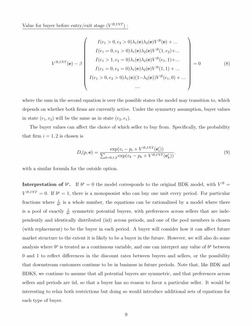
Value for buyer before entry/exit stage (V B,INT ) :
V B,INT (e)− β
I(e1 > 0, e2 > 0)λ1(e)λ2(e)V B(e) + ...
I(e1 = 0, e2 > 0)λ1(e)λ2(e)V B(1, e2)+...
I(e1 > 1, e2 = 0)λ1(e)λ2(e)V B(e1, 1)+...
I(e1 = 0, e2 = 0)λ1(e)λ2(e)V B(1, 1) + ...
I(e1 > 0, e2 > 0)λ1(e)(1−λ2(e))V B(e1, 0) + ...
....
= 0 (8)
where the sum in the second equation is over the possible states the model may transition to, which
depends on whether both firms are currently active. Under the symmetry assumption, buyer values
in state (e1, e2) will be the same as in state (e2, e1).
The buyer values can affect the choice of which seller to buy from. Specifically, the probability
that firm i = 1, 2 is chosen is
Di(p, e) =exp(vi − pi + V B,INT (e′i))∑
k=0,1,2 exp(vk − pk + V B,INT (e′k)). (9)
with a similar formula for the outside option.
Interpretation of bp. If bp = 0 the model corresponds to the original BDK model, with V B =
V B,INT = 0. If bp = 1, there is a monopsonist who can buy one unit every period. For particular
fractions where 1bp
is a whole number, the equations can be rationalized by a model where there
is a pool of exactly 1bp
symmetric potential buyers, with preferences across sellers that are inde-
pendently and identically distributed (iid) across periods, and one of the pool members is chosen
(with replacement) to be the buyer in each period. A buyer will consider how it can affect future
market structure to the extent it is likely to be a buyer in the future. However, we will also do some
analysis where bp is treated as a continuous variable, and one can interpret any value of bp between
0 and 1 to reflect differences in the discount rates between buyers and sellers, or the possibility
that downstream customers continue to be in business in future periods. Note that, like BDK and
BDKS, we continue to assume that all potential buyers are symmetric, and that preferences across
sellers and periods are iid, so that a buyer has no reason to favor a particular seller. It would be
interesting to relax both restrictions but doing so would introduce additional sets of equations for
each type of buyer.
9

2.1 Methods for Finding Equilibria
BDK and BDKS use two computational approaches to finding equilibria. The first approach fol-
lows Pakes and McGuire (1994) who use an iterative algorithm, where optimal prices/continuation
probabilities are computed and values are updated in each step, to find an equilibrium. The second
approach uses homotopies, which are essentially implementations of the implicit function theorem
to the system of equations that define an equilibrium, to trace equilibrium correspondences through
the strategy and value space as a single parameter is varied, starting from an equilibrium found
by the Pakes-McGuire algorithm or a homotopy where a different parameter was varied. An “α-
homotopy” is a homotopy where the equilibrium is traced varying parameter α. An advantage of
the homotopy approach is that it can identify equilibria that, because of the failure of local stability
conditions, cannot be found using the Pakes-McGuire algorithm unless one started exactly at the
equilibrium. However, even when the homotopy approach is applied repeatedly and varying differ-
ent parameters, it is not guaranteed to find all equilibria.10 Therefore, if only one equilibrium is
found for given parameters, it is unclear how confidently a researcher can claim that the equilibrium
is unique.
In this paper we also make use of the homotopy approach, with our implementation detailed
in Appendix A, including the criteria that we decide when similar numerical solutions should be
counted as different equilibria.11 However, because we want to make claims about how strategic
buyer behavior can lead to uniqueness, we also make use of a different approach which can show
whether equilibria where play must end up in particular absorbing states exist. To be precise, we
consider two types of equilibria where the game must terminate at states (M,M), (M, 0) or (0,M).
Definition An equilibrium is accommodative if the continuation probabilities λ1(e) = λ2(e) = 1
for all states e > (0, 0).
Definition An equilibrium has the“Some Exit Leads to Permanent Monopoly” (SELPM) property
if there is some e = (e1, e2) where e1 > e2 > 0, and (i) λ2(e) < 1, (ii) λ2(e′1, 0) = 0 and λ1(e
′1, 0) = 1
for all e′1 ≥ e1, and (iii) λ1(e′1, e′2) = 1 for all e′1 ≥ e1, e
′2 ≥ e2.
BDK2 define accommodative equilibria in the same way. In an accommodative equilibrium it is
10For example, BDK1, page 880: “Although it cannot be guaranteed to find all equilibria, the advantage of thismethod is its ability to explore the equilibrium correspondence and search for multiple equilibria in a systematicfashion.”
11Some of our numerical choices (e.g., tolerances) may differ from those of BDK or BDKS, but as we show ourresults appear almost identical for bp = 0.
10
certain that the game will eventually end up in state (M,M), where both firms are at the bottom
of their cost curves. By examining best response pricing functions as part of a backwards induction
algorithm, we find that, for all of the parameters considered, at most one accommodative equilibrium
can exist (see Appendix B). It is straightforward to check if an accommodative equilibrium exists
by solving for equilibrium prices assuming no exit, and then verifying that no exit is optimal.
Our definition and analyses of SELPM equilibria are new. The requirement is that there exists
a duopoly state e with the property that, once that state is reached, there is some probability that
the laggard will exit and, if it does, there is no probability of further entry, while the leader will
never exit. These restrictions imply that once the game leaves e it cannot return, and it must end
up in one of the absorbing states (M,M), (M, 0) or (0,M). As discussed in Appendix B, as long
as we are able to find all equilibria in a given state for a given set of buyer and seller continuation
values when the state changes, a recursive algorithm will be able to identify if such a state e exists
and therefore if a SELPM equilibrium exists.12 An extended version of this recursive algorithm can
also identify the existence of equilibria that any exit in the game will lead to permanent monopoly
(AELPM) (the formal definition of an AELPM equilibrium is also provided in Appendix B). All
AELPM equilibria are SELPM.
We can use the algorithms detailed in Appendix B to check, for given parameters, whether
an accommodative or any SELPM equilibria exist. We can also classify the equilibria identified
by homotopies as accommodative or SELPM. The value of being able to prove whether SELPM
equilibria exist comes from the fact that, for all of the parameters that we consider in this paper for
BDK model, as long as there is no exit when both firms are at the bottom of their learning curves
(i.e., in states (e1 ≥ m, e2 ≥ m)), all of the equilibria that the homotopies identify for all values of
bp are either accommodative or SELPM. Therefore showing, without relying on homotopies, that no
SELPM equilibria exist for particular parameters provides new evidence that no non-accommodative
equilibrium exist.13 From a policy perspective, it is also relevant to identify whether equilibria which
12Specifically, we can identify the existence of a SELPM equilibrium by following all equilibrium paths consistentwith SELPM until we find a state e or determine that no such state exists. A feature of the algorithm is that weknow that a SELPM equilibrium exists once we identify a state e, without having to solve the whole game, becausethe structure of the game implies that it is always possible to reach any duopoly state when a game starts at (1,1),and that an equilibrium in states with lower know-how that e must exist.
13Note we are not claiming that all non-accommodative equilibria will be SELPM if we considered a broader setof parameters. In particular, if there is some probability that the drawn entry costs are zero or very small therewill always be some probability of re-entry. In this sense, the assumption that entry costs are drawn from triangulardistributions is important to our approach. On the other hand, incentives to price aggressively and achieve dominance,which are the types of behavior that this literature has been most interested in, will also be substantially diminishedwhen entry is always likely.
11

may result in permanent monopoly (SELPM equilibria) exist.
3 The Effects of Strategic Buyers on Equilibrium Out-
comes for the Baseline Parameters
Before presenting our results across wide ranges of values for σ (product differentiation), ρ (learning
progress ratio) and bp, we show how equilibrium behavior and outcomes vary with bp when σ = 1
and ρ = 0.75, which form the baseline parameters in BDK1 and BDK2.14 This analysis will provide
the intuition for the changes in equilibrium behavior that we observe for a very broad range of
parameters.
3.1 Three Baseline Equilibria for bp = 0
There are three equilibria that can be supported for these parameters. Table 1 reports the strategies
for a sub-sample of states. We distinguish the equilibria by the expected long-run HHI (HHI∞)
implied by firm strategies assuming that game begins in state (1,1). BDK define HHI∞ as
HHI∞ =∑
e≥(0,0)
µ∞(e)
1− µ∞(e)HHI(e)
where
HHI(e) =∑i=1,2
(Di(p, e)
D1(p, e) +D2(p, e)
)2
and µ∞(e) is the probability that the game is in state e in the ergodic distribution. In any accom-
modative equilibrium, the ergodic distribution contains only state (M,M), where the HHI is 0.5,
so HHI∞ is also 0.5. The two non-accommodative equilibria are SELPM15, and the game ends up
in one of the states (M, 0), (0,M) (HHI is 1) or (M,M), so the long-run HHI simply reflects the
relative probability of these states.16
The three equilibria differ only in strategies where one or both firms have not made a sale, i.e.,
where at least one e is equal to 0 or 1. Once both firms have made a sale there is no possibility
14For the remaining parameters: κ (cost the top of the learning curve) is 10, X (scrap value) has a symmetrictriangular distribution on [0, 3], S (entry cost) has a symmetric triangular distribution on [3, 6].
15In these equilibria there is some probability of exit when one of the firms is in state 1 and the other has acquiredknow-how, but no probability that the leader exits and no probability of re-entry. State (30, 1) satisfies the definitionof e in the SELPM definition.
16BDK1 actually calculate HHI∞ based on the probability distribution of states after 1,000 periods (see BDK1,p. 883).
12

Tab
le1:
Equilib
ria
inth
eB
DK
Model
for
the
Bas
elin
eP
aram
eter
s
Hig
h-H
HI
Eqm
.M
id-H
HI
Eqm
.A
ccom
mod
ativ
eE
qm
.
(HHI∞
=0.
96)
(HHI∞
=0.
6)(HHI∞
=0.
5)e 1
e 2c 1
c 2p1
p2
λ1
λ2
p1
p2
λ1
λ2
p1
p2
λ1
λ2
11
10
10-3
4.78
-34.
780.
9996
0.99
963.
273.
271
15.
055.
051
12
18.5
10
0.08
3.63
10.
7799
3.62
4.65
10.
9998
5.34
6.29
11
31
7.7
310
0.5
64.
151
0.77
913.
444.
951
0.98
745.
456.
651
13
27.7
38.5
5.6
15.
941
15.
615.
941
15.
615.
941
14
17.2
310
0.8
04.
411
0.77
873.
385.
121
0.97
675.
516.
821
14
27.2
38.5
5.5
56.
061
15.
556.
061
15.
556.
061
14
47.2
37.2
35.6
55.
651
15.
655.
651
15.
655.
651
110
15.
8310
1.21
4.86
10.
7778
3.38
5.46
10.
9586
5.59
7.12
11
102
5.83
8.5
5.44
6.28
11
5.44
6.28
11
5.44
6.28
11
1010
5.83
5.83
5.32
5.32
11
5.32
5.32
11
5.32
5.32
11
291
3.25
101.
244.
901
0.77
773.
395.
491
0.95
775.
587.
151
129
23.
258.
55.
426.
301
15.
426.
301
15.
426.
301
130
13.
2510
1.24
4.90
10.
7777
3.39
5.49
10.
9577
5.58
7.15
11
302
3.25
8.5
5.42
6.30
11
5.42
6.30
11
5.42
6.30
11
3029
3.25
3.25
5.24
5.24
11
5.24
5.24
11
5.24
5.24
11
3030
3.25
3.25
5.24
5.24
11
5.24
5.24
11
5.24
5.24
11
10
10
-8.
80-
10
7.55
-1
0.13
578.
19-
10.
8816
20
8.5
-8.
72-
10
8.72
-1
08.
45-
10.
5233
100
5.83
-8.5
6-
10
8.56
-1
08.
55-
10.
2953
01
-10
-8.
800
1-
7.55
0.13
571
-8.
190.
8816
10
2-
8.5
-8.
720
1-
8.72
01
-8.
450.
5233
10
3-
7.73
-8.
680
1-
8.68
01
-8.
520.
4227
10
4-
7.23
-8.
650
1-
8.65
01
-8.
540.
3739
10
10
-5.
83-
8.56
01
-8.
560
1-
8.55
0.29
531
029
-3.
25-
8.54
01
-8.
540
1-
8.54
0.28
991
030
-3.
25-
8.54
01
-8.
540
1-
8.54
0.28
991
Note
s:c i
,pi,λi
are
the
mar
gin
al
cost
s,eq
uil
ibri
um
pri
cean
deq
uil
ibri
um
pro
bab
ilit
yof
conti
nu
ing
tob
ein
the
ind
ust
ryin
the
nex
tp
erio
dof
firm
i.HHI∞
isth
eex
pec
ted
lon
g-ru
nva
lue
ofth
eH
HI.
13

of exit on the equilibrium path and pricing strategies are identical across all three equilibria. The
two equilibria that involve exit involve lower equilibrium prices when one firm has not yet made a
sale. Intuitively, the possibility that a rival will exit if it does not make a sale provides the leader
with an incentive to try to make sure that the rival does not win the next sale, and, in turn, a low
probability that the rival will make a sale makes it more attractive for the rival to exit.
3.2 Effect of Changes in bp on Buyer Behavior Holding Seller StrategiesFixed
To illustrate the effect of strategic buyers, we analyze what happens when we increase bp holding
(unless otherwise noted) seller strategies fixed at their bp = 0 equilibrium values. Where necessary
for a calculation, we assume that the game begins in state (1,1).
Figure 2(a) shows the inverse demand for firm 1 (the leader) in state (3,1) as a function of bp for
the three sets of equilibrium seller strategies.17 In each of the two non-accommodative equilibria the
buyer can play a pivotal role in the evolution of the industry in the sense that, if it buys from firm 2,
the industry will be a duopoly forever and future pricing will be the same as in the accommodative
equilibrium. As the difference between expected future buyer surplus under monopoly and duopoly
is quite large, strategic buyer behavior has quite substantial effects on demand in the High-HHI
equilibrium, where laggard exit is reasonably likely if the leader makes the sale, even when bp is
fairly small. For example, at the bp = 0 equilibrium prices, the probability that the leader makes the
sale falls from 0.973 to 0.695 as bp increases from 0 to 0.1. In contrast, in the mid-HHI equilibrium,
where laggard exit is less likely, the effect on demand is significantly smaller (change is 0.818 to
0.759), and the effect is smaller still (0.762 to 0.727) in the accommodative equilibrium unless bp is
close to 1.18
Figure 2(b) illustrates how these changes in demand, and similar changes in other low know-how
states, affect the distribution of states after 10 periods of the game. With seller strategies fixed,
changes reflect only changes in buyer purchase choices. The figures distinguish between market
structures where one and two firms are active (monopoly and duopoly), and then, amongst the
duopoly states, it distinguishes between market structures according to the difference between the
know-how states of the duopolists. This figure shows that, in the High-HHI equilibrium, changes
17When we vary p1, the players assume that p1 will have its equilibrium value if the game is in state (3,1) in anyfuture period.
18In the accommodative equilibrium, the buyer improves future buyer surplus by buying from either firm, and itreduces expected future prices slightly by buying from the laggard.
14

Figure 2: Extended BDK Model: Outcomes as a Function of bp For Baseline Parameters and bp = 0Seller Strategies.
(a) Inverse Demand Curves For Seller 1 in State (3,1)
(b) Distribution of States after 10 Periods. The range of the duopoly state indicates the difference in thestates of the two active firms after 10 periods, so that, for example, if the game is in state (e1 = 7, e2 = 2)then it would count as being in the “Duopoly: 4-5” category.
15

Figure 2: Extended BDK Model: Outcomes as a Function of bp For Baseline Parameters and bp = 0Seller Strategies.
(c) Firm 1 Advantage-Building and Advantage-Denying Incentives in State (3,1). The baseline equilibriaare marked by H = High-HHI, M = Mid-HHI and A = Accommodative.
in buyers’ choices change the distribution of states significantly even when bp is only increased to
0.1. The changes in the other equilibria are much more modest unless bp is increased to 1.
Figure 2(c) shows how the changes in demand and the distribution of states associated with
increases in bp affect firm 1’s incentives to win the sale in state (3, 1). We follow BDK in breaking
the future benefit that a firm gets when it makes a sale into two different components.
Definition The advantage-building incentive for firm 1 is V S,INT1 (e1 + 1, e2) − V S,INT
1 (e1, e2).
The advantage-denying incentive for firm 1 is V S,INT1 (e1, e2)− V S,INT
1 (e1, e2 + 1).
The advantage-building incentive therefore measures the increase in a firm’s value that results
from it making a sale, versus no firm making a sale (and the state therefore remaining unchanged),
whereas the advantage-denying incentive reflects the increase in a firm’s value if no sale is made
by either firm, versus the rival making a sale. When there is duopoly, both incentives affect a
firm’s pricing decision, and, given the value of the outside option assumed by BDK, the most likely
outcomes are that either the firm makes the sale or the rival makes the sale. BDK1 show that
16

when the advantage-denying incentive is removed from firms’ pricing incentives that equilibrium
multiplicity is substantially reduced and that accommodative equilibria survive.19 It is therefore
relevant to ask how strategic buyer effective affects the advantage-denying incentive, in particular.
The figure is drawn assuming baseline seller strategies in all states but allowing for buyer demand
to change in all states reflecting different values of bp. In the High-HHI equilibrium, the advantage-
denying incentive is much larger than the advantage-building incentive when bp = 0, but it falls
quite rapidly for small increases in bp reflecting the fact that even if firm 2 does not win in the
current period, the changes in buyer demand will make it more likely to win in future periods if it
remains in the market. This is the case even though, with seller strategies fixed, there remains a
reasonable probability that the laggard will exit if it does not make the sale in the current period.
In contrast, all of the other incentives, which are much smaller, decline only slightly, and more
linearly, when bp is increased.
3.3 Effect of Changes in bp on Equilibrium Strategies
We next examine how equilibrium seller strategies change with bp, allowing for buyer strategies
to change as well. We do so using “bp-homotopies” starting at the three baseline equilibria. The
homotopies track the value of each strategy as bp changes.
Figure 3(a) shows the probabilities that firm 2 (the laggard) continues (i.e., does not exit) in
state (4,1), the state to which the industry moves if the leader makes the sale in state (3,1). The
figure shows that, in the bp dimension, the High-HHI and Mid-HHI equilibria are connected, so that
as bp is increased, the continuation probabilities rise or fall depending on which equilibrium is used
as a starting point. This section of the equilibrium correspondence does not reach beyond 0.142,
so that, for higher values, only an accommodative equilibrium, where firm 2 is certain to continue,
exists.
Figures 3(b) and 3(c) show what happens to equilibrium prices in state (3,1) and the leader’s
advantage-building and advantage-denying incentives. Starting from the High-HHI equilibrium, the
leader’s equilibrium price falls as bp increases from 0, reflecting its falling demand. Simultaneously,
however, the advantage-denying incentive is reduced as firm 2 is more likely to continue, and, once
it has fallen sufficiently, the leader prefers to set a higher price. The prices of the laggard vary less.
In the accommodative equilibrium, the prices of both firms rise in bp, as the advantage-building and
19See, for example, BDK1, Figure 3, where the removal of the advantage-denying incentive corresponds to Definition2/Panel B, where the surviving equilibria are accommodative.
17

Figure 3: Extended BDK Model: Equilibrium Outcomes as a Function of bp. The baseline equilibriaare marked by H = High-HHI, M = Mid-HHI and A = Accommodative.
(a) Equilibrium Probabilities that Firm 2 Continues in the Market in State (4,1). The black dashed linetraces the path of the bp homotopy from the Accommodative baseline equilibrium. The pink line tracesthe path of the bp homotopies starting at the other equilibria (the paths from each equilibrium overlap).
(b) Equilibrium Prices in State (3,1). The black and grey dashed lines trace the path of the bp homotopyfrom the Accommodative baseline equilibrium. The red and pink lines trace the paths of the bp homotopiesstarting at the other equilibria (the dashed and solid lines overlap).
18

Figure 3: Extended BDK Model: Equilibrium Outcomes as a Function of bp. The baseline equilibriaare marked by H = High-HHI, M = Mid-HHI and A = Accommodative.
(c) Equilibrium Advantage-Building and Advantage-Denying Incentives for Firm 1 in State (3,1).
advantage-denying incentives are reduced by the fact that buyers will favor the laggard in future
periods.
As noted, the bp-homotopies from the non-accommodative baseline equilibria do not continue
beyond bp = 0.142. However, as explained above, this does not necessarily imply that there is
only an accommodative equilibrium because there could be a separate, disconnected section of the
equilibrium correspondence that is not linked to the baseline equilibria where exit may occur. We
therefore use our recursive algorithm to test if any SELPM equilibrium exists. When we increase bp
from 0 to 1 in steps of 0.01, we find that, consistent with the homotopy figures, a SELPM equilibrium
exists for values of bp up to 0.14 (here the homotopies had found two SELPM equilibria), and that
no SELPM equilibrium exists for values above 0.15. This result also provides evidence that the
homotopy method does not miss equilibria when bp ≥ 0.15.
19

Figure 4: Extended BDK Model: Equilibrium Expected Long-Run HHI and Prices as a Functionof bp. The pink, blue dashed and black dashed lines trace homotopy paths from the High-HHI,Mid-HHI and Accommodative Equilibria respectively.
(a) Expected Long-Run HHI (HHI∞).
(b) Expected Long-Run Prices (p∞)
20
3.4 Effect of Changes in bp on Equilibrium Outcomes
Figure 4(a) shows the value of HHI∞ when we run bp-homotopies from the baseline equilibrium
outcomes. Consistent with the reverse of Figure 3(a), concentration in the High-HHI equilibrium
is reduced as bp increases from zero, while concentration in the Mid-HHI equilibrium increases,
but only the accommodative equilibrium survives once bp is increased past 0.142. The figure for
the expected long-run price, Figure 4(b), looks very similar. In all of the computed equilibria the
long-run state is (M,M), (M, 0) or (0,M). In these states equilibrium prices are independent of bp,
because the absorbing nature of these states implies that strategic buyers cannot affect the state
in the future, so that variation in expected long-run prices (or long-run consumer surplus), either
across equilibria or across values of bp, depends only on how bp affects the probability of these
different long-run outcomes. This, of course, is also what drives the variation in HHI∞.
The comparisons of the NPV of surplus are more interesting, as SELPM equilibria may have
higher consumer surplus in the early stages of a game, even if monopoly is more likely to emerge.
Figure 5 presents figures that show how the NPV of consumer surplus and total surplus using
the bp-homotopies, for games starting in state (1, 1).20 The NPV of total surplus is higher in the
accommodative equilibrium, but the NPV of consumer surplus when bp = 0 is maximized in the mid-
HHI equilibrium and minimized in the high-HHI equilibrium. The softening of initial competition in
the accommodative equilibrium as bp increases also causes consumer surplus in the accommodative
equilibrium to fall.
4 Results for the Extended BDK Model Across Values of
ρ and σ
We now examine how these patterns generalize for other parameters. Specifically, we consider what
happens when bp, ρ, the progress ratio, which determines the extent of LBD, and σ, which measures
the degree of product differentiation, vary. When product differentiation falls, equilibrium duopoly
profits tend to shrink, which tends to lead to more exit. When ρ falls (more LBD), there are two
effects. First, lower costs tend to increase duopoly profits making exit less attractive. On the
other hand, a firm that makes initial sales gains a larger cost advantage, which may increase the
20BDK1 calculates welfare assuming that the game starts in state (1,1), whereas BDK2 calculate welfare assumingthe game starts in state (0,0), so that initial entry costs are included and the possibility that there is never duopolyis accounted for. While both measures are interesting, we focus on NPV measures assuming that the game starts in(1,1) as antitrust analysis is typically focused on settings where there is actual competition during the initial stagesof an industry’s development.
21
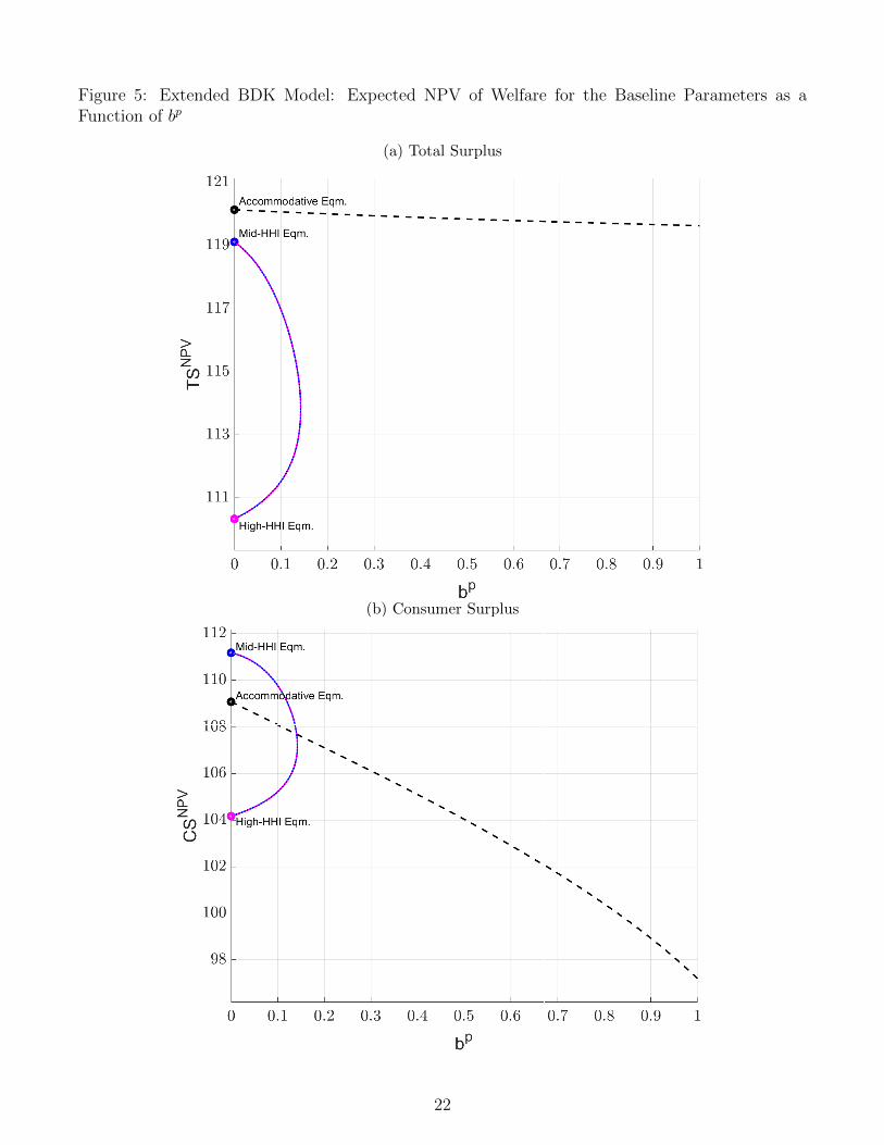
Figure 5: Extended BDK Model: Expected NPV of Welfare for the Baseline Parameters as aFunction of bp
(a) Total Surplus
(b) Consumer Surplus
22

probability that the laggard exits.
4.1 Long-Run Market Structure and Multiplicity of Equilibria
We first analyze how the parameters and bp affect long-run market structure, measured by HHI∞,
and the existence of multiple equilibria. Figure 6(a) (which matches BDK1 Figure 2, Panel B) shows
the HHI∞ path traced by a σ-homotopy when bp = 0 and ρ = 0.75. The other parameters are
held at their baseline values. When σ > 1.12 (high differentiation), there is only an accommodative
equilibrium (HHI∞ = 0.5), but otherwise at least one equilibrium exists where a firm may exit
and the market can end up as a monopoly. For σ < 0.9, all of the equilibria have a high probability
of monopoly (HHI∞ at or very close to 1), and, as a result of the homotopy path bending back
on itself, there can be many equilibria. For example, for σ = 0.8 there are 23 equilibria, all with
HHI∞ ≥ 0.95.21 All of the equilibria computed with HHI∞ > 0.5 are SELPM.
Figure 6(b) shows how the σ-homotopies change as bp increases. The main patterns are that, as
bp increases, the homotopies unwind, reducing multiplicity, and accommodative equilibria can be
supported for lower σ. When bp > 0.7, a high value, no equilibria has an HHI∞ close to 1 for any
σ ≥ 0.5.
Figure 7 presents similar plots for ρ-homotopies (matching BDK1 Figure 2, Panel A), with
the other parameters at their baseline values, including σ = 1. Recall that ρ = 1 corresponds to
no LBD, whereas as ρ → 0 marginal costs fall to zero once the firm has made one sale, so that
moving from left to right is associated with increasing LBD effects. For all ρ and for all bp, there
is an accommodative equilibrium (HHI∞ = 0.5), while, for bp = 0 and ρ ≤ 0.8, there are also
equilibria where exit occurs and the equilibrium correspondence has (at least in this dimension)
two disconnected loops. As bp increases, the geometry changes. The loops with the highest HHI∞
are eliminated as soon as bp ≥ 0.05, whereas the loops covering lower values of HHI∞ contract to
cover a smaller range of ρ, and they disappear entirely for bp > 0.3 (for the baseline ρ = 0.75 this
equilibrium disappears for bp ≥ 0.15, consistent with the σ-homotopy results). For bp > 0.3, only
the accommodative equilibrium exists for all values of ρ.
Figure 8 classifies the equilibrium identified by the σ- and ρ- homotopies into accommodative,
SELPM and AELPM equilibria, where the latter two groups are also broken down into whether
the equilibrium meets BDK2’s definition of an aggressive equilibrium (which involves a condition
21In all of these equilibria there is no exit when a firm has know-how level of six or higher, and for these stateswhere there are two active firms with know-how above 6 all of these equilibria have identical pricing strategies.
23
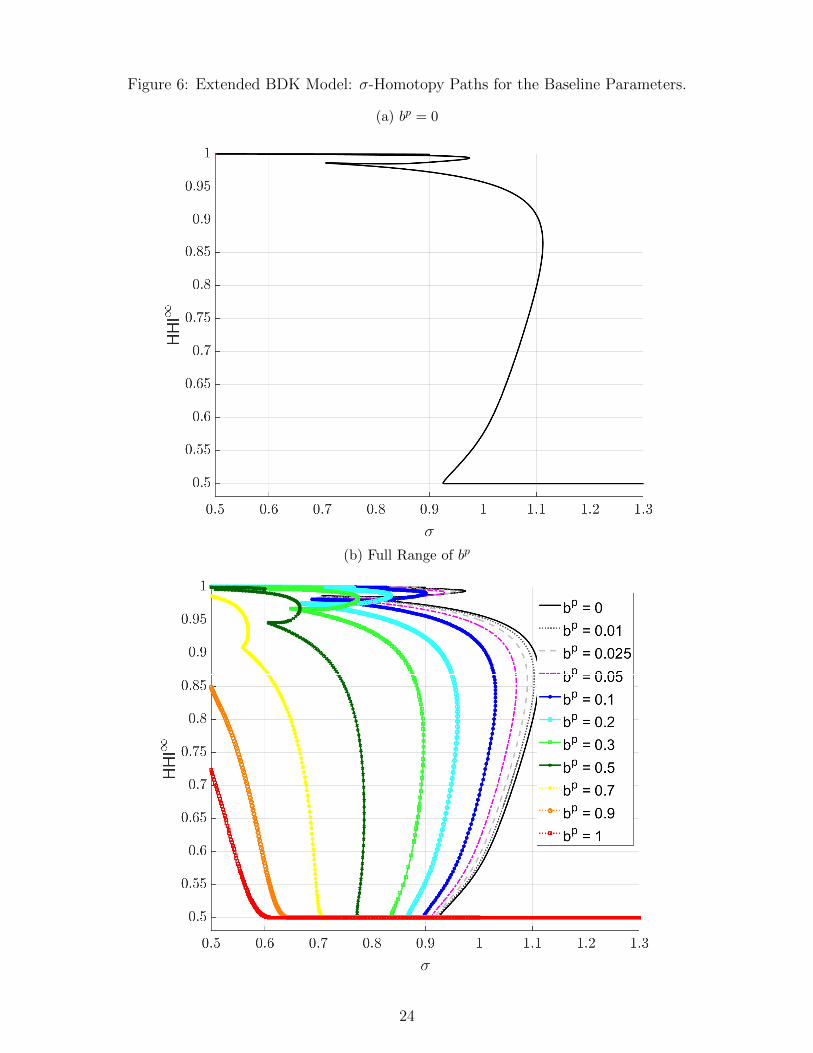
Figure 6: Extended BDK Model: σ-Homotopy Paths for the Baseline Parameters.
(a) bp = 0
(b) Full Range of bp
24

Figure 7: Extended BDK Model: ρ-Homotopy Path for Full Range of bp and the Baseline Parame-ters.
25

Figure 8: Extended BDK Model: Classification of Equilibria Identified by Homotopies for theBaseline Parameters and Full Range of bp
(a) ρ-Homotopy Paths
(b) σ-Homotopy Paths
26
on pricing as well as exit).22 Recall that AELPM equilibria are SELPM equilibria where any exit
from duopoly results in permanent monopoly.
There are two noticeable patterns. First, all of the equilibria that the homotopies identify in
these figures are either accommodative or SELPM (i.e., for these parameters the classificiation is
exhaustive), whereas some SELPM equilibria, and some AELPM equilibria, are not aggressive, i.e.,
some equilibria are unclassified using the aggressive/accommodative classification. Second, AELPM
equilibria tend to have lower HHI∞ values than non-AELPM SELPM equilibria. This may seem
like a counter-intuitive result as one might expect that equilibria where there is never any re-entry
after exit would involve more aggressive pricing and a more concentrated market structure. It is the
case that equilibria with very aggressive pricing tend to have the most concentrated structures. But,
in these equilibria, exactly because competition is intense, it may be optimal for a firm to choose to
exit, if it draws a large enough scrap value, when it has the same know-how as its rival. If so, then,
as a result of the incomplete information structure on entry/exit choices, both firms may exit, after
which re-entry can be optimal (as the potential entrants will have the chance to be monopolists). As
a result, these equilibria will not meet the AELPM definition, although they may be SELPM. If all
equilibria are accommodative or SELPM, a claim consistent with our classification of the homotopy
equilibria, then our recursive algorithm can prove whether an accommodative equilibrium is the
unique equilibrium.
The results of this analysis are shown in Figure 9 for a grid of values, in steps of 0.05, of (ρ, σ).
The only gridpoints for which neither accommodative nor SELPM equilibria exist are (ρ = 1,
σ ≤ 0.65), so that firms are always symmetric with high costs (no LBD) and there is little product
differentiation. For these parameters, equilibrium profits are low in every state, there is no role for
strategic buyer behavior (all states are the same) and exit may always be optimal for a duopolist.23
For the remaining combinations of parameters, there is a clear pattern. For bp = 0, there is a
large range of the parameter space where accommodative and SELPM equilibria co-exist, while it is
only when LBD has limited effects on costs (ρ large) that accommodative equilibria are the unique
equilibria for a wide range of σ.24 As bp increases, the ranges of parameters that support only an
accommodative equilibrium expands, whereas the range that supports SELPM equilibria shrinks,
22The equilibrium is aggressive if p1(e) < p1(e1, e2 + 1), p2(e) < p2(e1, e2 + 1), and λ2(e) < λ2(e1, e2 + 1) for somestate e > (0, 0) with e1 > e2, where λ is the probability of continuing.
23As firms may exit even when they both have the same nominal know-how, it is always possible to get some exitand some re-entry. This contradicts the definition of a SELPM equilibrium.
24See Appendix B for our evidence that there is only ever a single accommodative equilibrium.
27

Fig
ure
9:E
xte
nded
BD
KM
odel
:C
lass
ifica
tion
ofth
eT
yp
esof
Equilib
ria
that
Exis
tfo
r(ρ,σ
)C
ombin
atio
ns.
Shad
ing:
Whit
e-
nei
ther
SE
LP
Mnor
acco
mm
odat
ive
equilib
ria
exis
t;L
ight
Gre
y-
auniq
ue
acco
mm
odat
ive
equilib
rium
exis
ts,
no
SE
LP
Meq
uilib
ria
exis
t;D
ark
Gre
y-
auniq
ue
acco
mm
odat
ive
equilib
rium
and
SE
LP
Meq
uilib
ria
co-e
xis
t;B
lack
-SE
LP
Meq
uilib
ria
exis
t,ac
com
modat
ive
equilib
ria
do
not
exis
t.
28

with the changes most dramatic when LBD is more important (ρ low). For example, when ρ = 0
(costs fall from 10 to zero with one sale), SELPM equilibria can be supported for σ ≤ 1.05 with
bp = 0, but the threshold falls to σ ≤ 0.85 when bp = 0.3. For the highest levels of bp, there is only
multiplicity in a very narrow range of σ with low levels of product differentiation.
4.2 Prices and Welfare
Finally, we consider what happens to equilibrium prices and welfare as bp increases.
Figure 10 presents σ- and ρ-homotopy plots for the average long-run prices as bp is varied.
For any ρ or σ in these figures, the accommodative equilibria have the lowest long-run average
prices. This reflects the logic discussed in the baseline case where in all equilibria, the long-run
state is (M,M) (lowest prices), (M, 0) or (0,M), and the accommodative equilibrium maximizes
the probability of the duopoly state. For the same reason, the plots resemble those for HHI∞,
except that ρ and σ also have direct effect on equilibrium prices (for example, low ρ implies lower
costs in all of the terminal states).
The comparisons are more complicated for the NPV measures of welfare. We draw Figures 11
and 12 for a subset of bp values because of the number of crossings, and, for the ρ-homotopies, we
express welfare relative to the unique (accommodative) equilibrium outcome when bp = 1 . The
diagrams distinguish between accommodative equilibria (solid lines) and SELPM equilibria (dashed
lines). For all ρ, with σ = 1, one pattern that is consistent with the baseline case, is that, when
multiple equilibria exist, the NPV of total surplus is maximized in the accommodative equilibrium,
whereas the NPV of consumer surplus in the accommodative equilibrium lies between values in
SELPM equilibria. Holding fixed the parameters, increasing bp tends to reduce consumer surplus
in accommodative equilibria due to the softening of price competition. This is also true for total
surplus except when ρ ≥ 0.9 (Figure 11(b)).
For 0.9 < ρ < 1, the pattern is different, although the differences in total surplus are not too
large. The intuition for this difference, is that marginal costs are high for these parameters in all
states, so that, when bp is small the probability that a buyer will take the outside option is higher
than in the baseline case. For example, when ρ = 0.925 and bp ≤ 0.2, the probability that the
buyer chooses the outside option in state (1, 1) is around 0.272. On the other hand, a strategic
buyer will recognize that buying from afirm will lower future costs, and therefore there will be
more transactions and higher total surplus (as long as the buyer’s valuation exceeds the marginal
29

Figure 10: Extended BDK Model: Long-Run Prices for Full Range of bp
(a) ρ-Homotopies
(b) σ-Homotopies
30

Figure 11: Extended BDK Model: NPV Welfare for Full Range of bp for ρ-Homotopies, with σ = 1.Solid lines indicate accommodative equilibria and dashed lines indicate SELPM equilibria.
(a) Consumer Surplus
(b) Total Surplus
31

Figure 12: Extended BDK Model: NPV Welfare for Full Range of bp for σ-Homotopies, withρ = 0.75.Solid lines indicate accommodative equilibria and dashed lines indicate SELPM equilibria.
(a) Consumer Surplus
(b) Total Surplus
32

opportunity cost of sale, including the dynamic benefit).25 Continuing the example, when bp = 1,
the probability that the buyer chooses the outside option falls to 0.241 (a 10% decrease).
For the σ-homotopies the pattern looks somewhat different as no accommodative equilibrium
exists for low values of σ unless bp is close to 1. The most noticeable pattern is that, even though
many SELPM equilibria can exist for lower values σ and low bp, they tend to generate similar NPV
welfare measures, reflecting the fact that all of the equilibria tend to result in permanent monopoly
quite quickly, after which equilibrium prices are the same.
5 Results from the Extended BDKS Model
As discussed in the context of the baseline example, a feature of SELPM equilibria in the BDK
model is that the nature of exit choices means that buyers in some states can play a pivotal role
in the evolution of the market. This helps to explain why even moderately-strategic buyers may
have strong incentives to favor a firm that may otherwise exit, changing seller incentives to price
aggressively, contributing to the elimination of equilibria that involve exit. This leads to the question
of whether strategic buyer behavior would have similar effects in a model where buyers can never
play such a pivotal role. We, therefore, consider the BDKS model where there is no exit and know-
how can stochastically depreciate by at most one unit in any period, so that, unlike in the the
typical equilibrium in the BDK model, it is always possible for either firm to move up its marginal
cost curve.
5.1 Differences Between the BDKS and BDK Models
In the BDKS model there are always two active firms, with no entry or exit decisions. Once the
buyer has made its purchase choice, which, unlike the BDK model, does not include an option not
to purchase26, know-how evolves according to
ei,t+1 = min(M,max(ei,t + qi,t︸︷︷︸≡1 if i makes sale
− fi,t︸︷︷︸≡1 if i forgets︸ ︷︷ ︸
indicators
))
25In the example, equilibrium prices for all bp are greater than marginal cost, so surplus is created when additionalsales are made.
26BDKS’s code actually does allow for the possibility of no purchase but this option is effectively eliminated bychoosing a v0 of -100. We will report measures of surplus relative to surplus when bp = 1 so that the chosennormalization of the utility of the outside option does not affect the reported results.
33

where fi,t is equal to one with probability ∆(ei) = 1− (1− δ)ei where δ ∈ [0, 1]. The δ parameter
therefore parameterizes the forgetting rate. σ is assumed to be equal to 1, with (ρ, δ) as the main
parameters of interest. A central insight of the BDKS paper is that, because forgetting can move
a firm up its cost curve, an increase in the rate of forgetting can have a quite different effect on
equilibrium strategies than a slower rate of learning.
5.2 BDKS Equilibria for Example Parameters
The differences in the structure of the games create some differences in the equilibria. Table 2 reports
strategies for a subset of states for three equilibria identified when bp = 0, ρ = 0.75 (facilitating
comparison with our BDK examples) and δ = 0.0275. We will use these parameters in some of our
discussion below.27 The table also reports the state-specific probabilities that a firm forgets (∆).
In all of the equilibria firms set negative prices in state (1,1), as they compete to get an advantage.
Unlike in the BDK model, the equilibria differ in strategies (and values) across all states rather than
just in a subset of states with low know-how. This is because in the BDKS model there is always
some possibility of the game returning to any state from any point in the game in equilibrium, so
differences in prices in some states tend to lead to differences in continuation values, and therefore
optimal strategies, in all states. The fact that forgetting can always occur also implies that there
are no terminal, absorbing states.
The first two equilibria involve very similar prices in states other than (1, 1) (although they all
differ when looking at the fourth or fifth decimal place) and the most noticeable feature of these
equilibria is a “sideways trench” where the price of the leading firm drops when its rival moves
from know-how level 1 to know-how level 2, but then, if the laggard gains additional know-how,
the leader’s price increases even though the laggard’s costs are falling. In the third equilibrium, the
firms set low prices when they are symmetric (i.e., when a sale may cause leadership to switch from
one firm to the other) and we call this case a “diagonal trench”. The table also reports HHI∞
for each equilibria. Despite the differences in the strategies, each of the equilibria has a relatively
unconcentrated market outcome in the long-run.28
27Appendix C will report some corresponding analysis for ρ = 0.85 and δ = 0.0275 which is one of the parametervalues that BDKS focus on in their analysis. For these parameters there are two equilibria, which is unusual, andone of them is characterized as “flat with well”, in the sense that the pricing functions are relatively flat across theknow-how space except that the firms set lower prices in state (1,1).
28In the BDK model, for all of the equilibria that we consider in this paper, the long-run HHI is either 0.5 or 1, andHHI∞ is equal to the weighted average of these outcomes. In the BDKS model all states have positive probabilityin the long-run when δ > 0.
34

Table 2: Equilibria in the BDKS Model for δ = 0.0275, ρ = 0.75 , bp = 0
Sideways Trench Sideways Trench Diagonal Trench
HHI∞ = 0.5000260 HHI∞ = 0.5000259 HHI∞ = 0.5209345e1 e2 c1 c2 ∆1 ∆2 p1 p2 p1 p2 p1 p21 1 10 10 0.028 0.028 -4.12 -4.12 -4.10 -4.10 -3.25 -3.252 1 7.50 10 0.054 0.028 4.86 7.52 4.86 7.52 5.05 7.652 2 7.50 7.5 0.054 0.054 2.87 2.87 2.87 2.87 0.21 0.213 1 6.34 10 0.080 0.028 6.22 8.87 6.22 8.87 6.61 8.963 2 6.34 7.5 0.080 0.054 4.13 5.38 4.13 5.38 3.84 5.813 3 6.34 6.34 0.080 0.080 4.61 4.61 4.61 4.61 1.34 1.344 1 5.63 10 0.106 0.028 6.31 8.91 6.31 8.91 6.72 8.834 2 5.63 7.50 0.106 0.054 4.65 6.01 4.65 6.01 5.29 7.014 3 5.63 6.34 0.106 0.080 4.71 5.25 4.71 5.25 3.63 5.354 4 5.63 5.63 0.106 0.106 4.93 4.93 4.94 4.94 1.67 1.6710 1 3.85 10 0.243 0.028 6.07 8.58 6.07 8.58 6.20 8.0410 2 3.85 7.5 0.243 0.054 4.91 6.05 4.91 6.05 5.59 6.3910 3 3.85 6.34 0.243 0.080 5.15 5.83 5.15 5.83 5.69 6.2710 8 3.85 4.22 0.243 0.200 4.99 5.13 4.99 5.13 4.35 5.7310 9 3.85 4.02 0.243 0.222 5.01 5.07 5.01 5.07 3.15 4.4110 10 3.85 3.85 0.243 0.243 5.04 5.04 5.04 5.04 2.44 2.4429 1 3.25 10 0.555 0.028 5.90 8.37 5.90 8.37 5.60 7.5129 2 3.25 7.5 0.555 0.054 4.81 5.79 4.81 5.79 5.06 5.6630 1 3.25 10 0.567 0.028 5.90 8.37 5.90 8.37 5.66 7.6030 2 3.25 7.5 0.567 0.054 4.81 5.79 4.81 5.79 5.07 5.72
Notes: ci, pi, ∆i are the marginal costs, equilibrium price and probability of forgetting for firm i. HHI∞
is the expected long-run value of the HHI.
35

5.3 Existence of Multiple Equilibria in the Extended BDKS Model
As forgetting can always cause a firm with know-how to move backwards through the state-space,
there are no absorbing terminal states and it is not possible to use a recursive algorithm to establish
whether equilibria of a particular type exist.29 We therefore follow BDKS in using a sequence of
δ- and ρ-homotopies to criss-cross the parameter space for different discrete values of bp, as well as
checking that these results are consistent with bp-homotopies that begin from bp = 0.30 The details
of our implementation of the homotopy algorithm are given in Appendix A.
Figure 13 compares a heat-map indicating the number of equilibria that we identify when bp = 0
for different (ρ, δ) with an equivalent figure taken from BDKS’s paper. Even though the grid points
that we use may not be identical to BDKS, the diagrams match almost exactly except for some
parameters in a small area where ρ > 0.97 and δ is around 0.04, where we identify some additional
equilibria. Multiplicity exists for a range of values of ρ when δ lies between 0.02 and 0.15. These
values of δ imply a probability of forgetting when ei = 15 (the point at which additional know-how
does not lower costs) of 0.26 and 0.91 respectively. When the probability of forgetting is above 0.5
it is, of course, not possible, even for a strategic monopsonist, to maintain both firms at the bottom
of their learning curves for a sustained period.
Figures 14 and 15 show our results when we repeat the criss-crossing exercise for a discrete set
of bp values 0.01, 0.05, 0.1 and 0.2. We find no multiplicity when bp = 1, so we do not show that
figure. While we find a few parameters where we find more equilibria with bp = 0.05 than we do
when bp = 0, the striking result is that multiplicity is eliminated quite rapidly, with multiplicity
only appearing in a small sliver of the parameter space once bp = 0.1. This sliver is associated with
parameters that are quite extreme in the sense they imply dramatic LBD (ρ = 0.2 implies that
c(1) = 10 and c(2) = 2) and a high probability of forgetting (if δ = 0.1 a firm with ei = 5 forgets
with probability 0.41). For bp = 0.2 we only find multiplicity for some extremely high values of δ
where it is very unlikely that a firm can move more than one step down the cost curve. Appendix
C presents examples using bp-homotopies confirming both the elimination of equilibria and the
existence of examples where the number of equilibria can increase for low bp.
To gain some understanding for why multiplicity disappears relatively quickly in the BDKS
29The exception is when δ = 0. In this case backwards induction can be used to prove uniqueness of an equilibrium.The argument is similar to the one that we describe for accommodative equilibria in the BDK model in AppendixB, but it is simplified because one firm must make a sale.
30δ- and ρ-homotopies are run sequentially using the new equilibria that are found in the last round on a discretegrid of (ρ, δ) values.
36

Figure 13: Extended BDKS Model: Number of Equilibria for bp = 0
(a) Our Analysis
0.01 0.03 0.05 0.1 0.2 1
0.1
0.2
0.3
0.4
0.5
0.6
0.7
0.8
0.9
1
13579
(b) BDKS’s original results
LEARNING, FORGETTING, AND INDUSTRY DYNAMICS 471
“backward” to a lower state and when δ = 1, it can never move “forward” to ahigher state. Hence, backward induction can be used to establish uniqueness ofequilibrium (see Section 7 for details). In contrast, when δ ∈ (0�1), a firm canmove in either direction. These bidirectional movements break the backwardinduction and make multiple equilibria possible:
PROPOSITION 4: If organizational forgetting is neither absent (δ = 0) nor cer-tain (δ= 1), then there may be multiple equilibria.
Figure 2 proves the proposition and illustrates the extent of multiplicity. Itshows the number of equilibria that we have identified for each combination ofprogress ratio ρ and forgetting rate δ. Darker shades indicate more equilibria.As can be seen, we have found up to nine equilibria for some values of ρ and δ.Multiplicity is especially pervasive for forgetting rates δ in the empirically rel-evant range below 0�1.
In dynamic stochastic games with finite actions, Herings and Peeters (2004)have shown that generically the number of MPE is odd. While they considerboth symmetric and asymmetric equilibria, in a two-player game with symmet-ric primitives such as ours, asymmetric equilibria occur in pairs. Hence, theirresult immediately implies that generically the number of symmetric equilibria
FIGURE 2.—Number of equilibria.
37

Figure 14: Extended BDKS Model: Number of Equilibria for bp > 0
(a) bp = 0.01
0.01 0.03 0.05 0.1 0.2 1
0.1
0.2
0.3
0.4
0.5
0.6
0.7
0.8
0.9
1
13579
(b) bp = 0.05
38

Figure 15: Extended BDKS Model: Number of Equilibria for bp > 0
(a) bp = 0.1
(b) bp = 0.2
39

model, we perform a similar analysis to the one used for the baseline parameters in the BDK
model, but using our example parameters from Section 5.2. This is presented in the three panels of
Figure 16, where, in each case, we allow buyer strategies to change as we increase bp, but hold seller
strategies fixed at the bp = 0 values (i.e., the prices in Table 2). The similarity between the two
sideways trench equilibria means that the figures for these equilibria are not visually distinguishable.
Figure 16(a) shows the inverse demand for firm one in state (3,1). In all of the three BDKS
equilibria shown, the shifts are larger than they were for the accommodative and Mid-HHI equilibria
in the BDK model. In each case there is an incentive for a strategic buyer to try to shift the game
to state (3,2) rather than (4,1): in the case of the sideways trench equilibria, state (3,2) is in the
trench with low prices, while in the diagonal trench equilibrium prices are lower when the firms are
symmetric. Figure 16(b) shows the distribution of states after ten periods of the game, starting in
(1,1), for different values of bp. Even though stochastic forgetting means that even a monopsonist
has limited control over how the state evolves, the effect of even limited strategic behavior is to
push the game towards outcomes where the firms are more symmetric.
As a result, the advantage-denying incentives of the leader, which, recall, BDK1 identify as being
important to maintain equilibria where firms set low prices to maintain an advantage, also tend
to decline quickly. This is shown in Figure 16(c).31 For all three equilibria the advantage-denying
incentives are larger than the advantage-building incentives when bp = 0, but they fall significantly
as bp increases.32 One feature that is different to our BDK examples is that the advantage-building
incentives are non-monotonic in bp and, in particular, they increase for low values of bp.33
5.4 Market Structure, Price and Welfare
Figures 17 and 18 show how expected long-run market concentration and average prices, and the
NPV of consumer and total surplus, measured relative to surplus when bp = 1, for a game starting
31Even though buyers do not have the option to purchase in the BDKS model, we continue to define the advantage-building incentives as the difference between firm 1’s continuation values when firm 1 makes a sale and the continu-ation value if there was no sale, and the advantage-denying incentive as the difference between firm 1’s continuationvalue when there is no sale and firm 2 makes the sale.
32While it is obviously not straightforward to compare the incentives across two different models, it is also noticeablethat the levels of the advantage-denying incentive when bp = 0 are lower in the three equilibria than the incentive inthe High-HHI equilibrium of the BDK model, reflecting the fact that, in the BDKS model, there is no possibility offirm 1 gaining a permanent monopoly position through firm 2 exiting.
33The most obvious intuition for this result is that, the probability that a strategic buyer will buy from the laggardis decreasing when the leader has more know-how and this may make the accumulation of know-how more valuablefor the leader as bp increases. On the other hand, once buyers are quite strategic, the probability that the leader willbe able to maintain a significant advantage will fall, decreasing the advantage-building incentive.
40

Figure 16: Extended BDKS Model: Outcomes as a Function of bp For Baseline Parameters andbp = 0 Seller Strategies.
(a) Inverse Demand Curves For Seller 1 in State (3,1)
(b) Distribution of States after 10 Periods. The range of the duopoly state indicates the difference in thestates of the two active firms after 10 periods, so that, for example, if the game is in state (e1 = 7, e2 = 2)then it would count as being in the “Duopoly: 4-5” category.
41

Figure 16: Extended BDKS Model: Outcomes as a Function of bp For Baseline Parameters andbp = 0 Seller Strategies.
(c) Firm 1 Advantage-Building and Advantage-Denying Incentives in State (3,1). The example equilibriaare marked by ST = Sideways Trench (2 equilibria) and DT = Diagonal Trench.
at (1,1), vary with δ and bp, based on δ-homotopies, holding ρ fixed at 0.75. Similar figures, but with
ρ varying rather than δ (with δ held fixed at 0.05, as the results are clearer than when δ = 0.0275)
are presented in Appendix C.
Consistent with our results for the number of equilibria, the folds and loops in the equilibrium
correspondences that are evident for low δ are eliminated as bp rises, so that there is a unique
equilibrium for all δ for bp ≥ 0.1. For δ < 0.6, increases in bp are associated with lower long-
run market concentration, consistent with the pattern identified in the BDK model that strategic
buyers spread purchases to preserve long-run competition. However, whereas in the BDK model
lower long-run concentration is associated with lower long-run prices because the game always ends
up in one of the states (M,M), (M, 0) or (0,M), in the BDKS model the possibility of forgetting
means that spreading sales may raise long-run production costs. This leads to long-run prices being
higher when bp = 1 than for some lower values when δ is between 0.03 and 0.1. On the other hand,
for higher values of δ, more strategic buyer behavior is associated with higher concentration and
42

Figure 17: Extended BDKS Model: Long-Run Expected HHI and Average Prices with ρ = 0.75.
(a) Expected Long-Run HHI (HHI∞)
(b) Long-Run Expected Prices (P∞)
43

Figure 18: Extended BDKS Model: NPV of Welfare in the with ρ = 0.75 (measured relative towelfare when bp = 1).
(a) Consumer Surplus
(b) Total Surplus
44

lower long-run prices, as strategic buyers focus their purchases on one firm to try to keep its costs
low.
The feature that competition to defend or attain an advantage can last indefinitely in the BDKS
model also affects the welfare comparisons. In the welfare plots we show a smaller number of bp
lines to avoid clutter. For low values of δ, such as δ = 0.0275, where there are multiple equilibria
when bp = 0, the effect of introducing small amounts of strategic buyer behavior depends on which
equilibrium is considered. This is consistent with the BDK model. Focusing on higher values of bp,
such as 0.1, where there is always a single equilibrium for the parameters shown, increasing bp tends
to lower consumer surplus and total surplus for δ < 0.6, although we note that the comparison is
unclear around δ = 0.2. For δ > 0.6, strategic buyer behavior increases welfare because, in the
presence of rapid forgetting, the strategic buyer can lower production costs by buying from the
leader.34 As an aside, we note that even though the lines in all of the figures intersect at δ = 0.6,
this value is not associated with the equilibrium strategies that are everywhere identical for different
values of bp. For example, for low values of bp, the equilibrium involves firms setting low prices when
their states are symmetric (a diagonal trench), whereas for higher values of bp there is there is a
range of states where firms have different levels of experience but prices are very low. However,
because the probability of forgetting is very high, the game will usually be played with both firms
having no or very low know-how, and for these states equilibrium prices are similar, leading to
similar values of HHI∞, P∞ and the NPV welfare measures.
6 Conclusion
We have examined how equilibrium behavior and market outcomes change in well-known models
where firms can benefit from learning-by-doing (LBD) when buyers partially internalize how their
purchase decisions affect future buyer surplus. Our examination is motivated by the fact that most
industries where LBD has been documented have a number of large, repeat buyers, whereas the
existing literature has focused on the polar cases of short-lived atomistic buyers and monopsony.
The literature that has assumed that buyers are atomistic has emphasized that the existence of
multiple equilibria is the norm rather than the exception, and that it is common for equilibria where
competition tends to persist to coexist with equilibria where the industry develops as a monopoly or
34For example, the probability that the firm forgets when it has acquired one level of know-how (ei = 2) is 0.84when δ = 0.6.
45

with a market structure that is close to monopoly. We find that even moderate degrees of forward-
looking buyer behavior eliminate the multiplicity of equilibria for most parameter values, and it is
equilibria where competition is more likely to be sustained in the long-run that survive. As a result,
strategic buyer behavior tends to lower prices in the long-run, even though the NPV of consumer
surplus can be lowered as the incentive of firms to try to gain an initial advantage is weakened.
We interpret our results as having encouraging implications for both policy and future applied
modeling of markets where LBD is present. One interpretation of the existing literature would be
that, left to themselves, industries where firms can benefit from LBD, might tend to tip towards
inefficient dominance by a single firm, even when the underlying demand and cost structure could
also support long-run competition. One response would be to try to design policy rules to prevent
aggressive pricing, but as BDK1 acknowledge, it is difficult to do so without the risk that beneficial
competitive conduct will also sometimes be prevented. Our results suggest that even moderate
degrees of forward-looking buyer behavior tend to eliminate equilibria where firms achieve domi-
nance, suggesting that the difficult policy design problem may often be unnecessary and that claims
of predatory behavior can also be treated more skeptically in markets with even moderate buyer-
side concentration. The existence of multiple equilibria also provides a well-known challenge, and
often a deterrent, to conducting empirical and other applied research, especially in models where we
have no reliable methods for collating equilibria. Our finding that equilibria with strategic buyers
are typically unique, which is confirmed using a new approach in the context of the BDK model,
suggests that adding strategic buyers may be a way to reduce multiplicity concerns, while also
increasing the realism of these models.
An important direction for future research will be to identify whether these encouraging results
are robust to including additional realistic extensions. For example, in most of the markets where
strategic buyers are relevant, buyers may be asymmetric in their size or tastes, buyers and sellers
may also be able to write contracts with multi-period options35, or prices may be set by some
combination of a procurement auction and subsequent negotiation with the preferred bidder. It
may be impractical to use homotopy methods to exhaustively search for multiple equilibria in
models that include these features, making the types of recursive method that we use in this paper
to confirm the homotopy results even more useful.
35One reason for preferring a model without commitment is that even if a buyer and seller sign a contract coveringmultiple periods when there is competition, there is some risk of ex-post opportunism by a seller that becomes amonopolist if there are non-contractible elements that firms care about.
46

References
Alchian, A. (1963): “Reliability of Progress Curves in Airframe Production,” Econometrica,31(4), 679–693.
Anton, J. J., G. Biglaiser, and N. Vettas (2014): “Dynamic Price Competition with Ca-pacity Constraints and a Strategic Buyer,” International Economic Review, 55(3), 943–958.
Asker, J., C. Fershtman, J. Jeon, and A. Pakes (forthcoming): “A Computational Frame-work for Analyzing Dynamic Procurement Auctions: The Market Impact of Information Sharing,”RAND Journal of Economics.
Benkard, C. L. (2000): “Learning and Forgetting: The Dynamics of Aircraft Production,” Amer-ican Economic Review, 90(4), 1034–1054.
(2004): “A Dynamic Analysis of the Market for Wide-Bodied Commercial Aircraft,” TheReview of Economic Studies, 71(3), 581–611.
Besanko, D., U. Doraszelski, and Y. Kryukov (2014): “The Economics of Predation: WhatDrives Pricing When There is Learning-by-Doing?,” American Economic Review, 104(3), 868–97.
(2019a): “How Efficient is Dynamic Competition? The Case of Price as Investment,”American Economic Review, 109(9), 3339–64.
(2019b): “Sacrifice Tests for Predation in a Dynamic Pricing Model: Ordover and Willig(1981) and Cabral and Riordan (1997) meet Ericson and Pakes (1995),” International Journal ofIndustrial Organization.
Besanko, D., U. Doraszelski, Y. Kryukov, and M. Satterthwaite (2010): “Learning-by-Doing, Organizational Forgetting, and Industry Dynamics,” Econometrica, 78(2), 453–508.
Board, S., and A. Skrzypacz (2016): “Revenue Management with Forward-Looking Buyers,”Journal of Political Economy, 124(4), 1046–1087.
Cabral, L. M., and M. H. Riordan (1994): “The Learning Curve, Market Dominance, andPredatory Pricing,” Econometrica, 62(5), 1115–1115.
Chen, Y., V. F. Farias, and N. Trichakis (2019): “On the Efficacy of Static Prices for RevenueManagement in the Face of Strategic Customers,” Management Science, 65(12), 5535–5555.
Dafny, L. S. (2005): “Games Hospitals Play: Entry Deterrence in Hospital Procedure Markets,”Journal of Economics & Management Strategy, 14(3), 513–542.
Dick, A. R. (1991): “Learning-By-Doing and Dumping in the Semiconductor Industry,” Journalof Law and Economics, 34(1), 133–159.
Ericson, R., and A. Pakes (1995): “Markov-Perfect Industry Dynamics: A Framework forEmpirical Work,” Review of Economic studies, 62(1), 53–82.
Gans, J. S., and S. P. King (2002): “Exclusionary Contracts and Competition for Large Buyers,”International Journal of Industrial Organization, 20(9), 1363–1381.
47

Gaynor, M., H. Seider, and W. B. Vogt (2005): “The Volume-Outcome Effect, ScaleEconomies, and Learning-by-Doing,” American Economic Review, 95(2), 243–247.
Horner, J., and L. Samuelson (2011): “Managing Strategic Buyers,” Journal of PoliticalEconomy, 119(3), 379–425.
Irwin, D. A., and P. J. Klenow (1994): “Learning-by-Doing Spillovers in the SemiconductorIndustry,” Journal of Political Economy, 102(6), 1200–1227.
Jerath, K., S. Netessine, and S. K. Veeraraghavan (2010): “Revenue Management withStrategic Customers: Last-Minute Selling and Opaque Selling,” Management Science, 56(3),430–448.
Kim, M. (2014): “Strategic Responses to Used Goods Markets: Airbus and Boeing,” Discussionpaper, University of Oklahoma.
Lewis, T. R., and H. Yildirim (2002): “Managing Dynamic Competition,” American EconomicReview, 92(4), 779–797.
Lewis, T. R., and H. Yildirim (2005): “Managing Switching Costs in Multiperiod Procurementswith Strategic Buyers,” International Economic Review, 46(4), 1233–1269.
Lieberman, M. B. (1984): “The Learning Curve and Pricing in the Chemical Processing Indus-tries,” RAND Journal of Economics, 15(2), 213–228.
(1987): “Patents, Learning by Doing, and Market Structure in the Chemical ProcessingIndustries,” International Journal of Industrial Organization, 5(3), 257–276.
Loertscher, S., and L. M. Marx (2019): “Merger Review for Markets with Buyer Power,”Journal of Political Economy, 127(6), 2967–3017.
Maskin, E., and J. Tirole (2001): “Markov Perfect Equilibrium: I. Observable Actions,” Journalof Economic Theory, 100(2), 191–219.
Pakes, A., and P. McGuire (1994): “Computing Markov-Perfect Nash Equilibria: NumericalImplications of a Dynamic Differentiated Product Model,” RAND Journal of Economics, 25(4),555–589.
Saini, V. (2012): “Endogenous Asymmetry in a Dynamic Procurement Auction,” RAND Journalof Economics, 43(4), 726–760.
Sweeting, A., J. W. Roberts, and C. Gedge (2020): “A Model of Dynamic Limit Pricingwith an Application to the Airline Industry,” Journal of Political Economy, 128(3), 1148–1193.
Sweeting, A., X. Tao, and X. Yao (2019): “Dynamic Games with Asymmetric Information:Implications for Mergers,” Discussion paper, University of Maryland.
Thompson, P. (2001): “How much did the Liberty Shipbuilders Learn? New Evidence for an OldCase Study,” Journal of Political Economy, 109(1), 103–137.
Thornton, R. A., and P. Thompson (2001): “Learning from Experience and Learning fromOthers: An Exploration of Learning and Spillovers in Wartime Shipbuilding,” American Eco-nomic Review, 91(5), 1350–1368.
48

Zimmerman, M. B. (1982): “Learning Effects and the Commercialization of New Energy Tech-nologies: The Case of Nuclear Power,” Bell Journal of Economics, 13(2), 297–310.
49
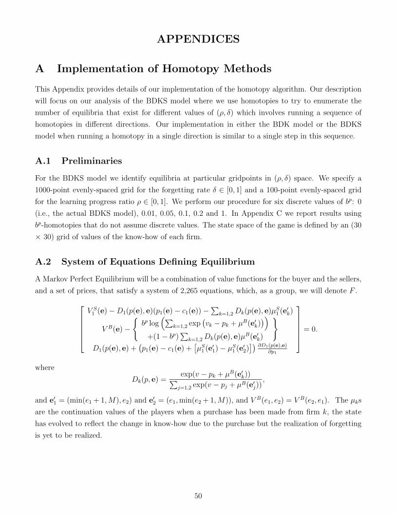
APPENDICES
A Implementation of Homotopy Methods
This Appendix provides details of our implementation of the homotopy algorithm. Our description
will focus on our analysis of the BDKS model where we use homotopies to try to enumerate the
number of equilibria that exist for different values of (ρ, δ) which involves running a sequence of
homotopies in different directions. Our implementation in either the BDK model or the BDKS
model when running a homotopy in a single direction is similar to a single step in this sequence.
A.1 Preliminaries
For the BDKS model we identify equilibria at particular gridpoints in (ρ, δ) space. We specify a
1000-point evenly-spaced grid for the forgetting rate δ ∈ [0, 1] and a 100-point evenly-spaced grid
for the learning progress ratio ρ ∈ [0, 1]. We perform our procedure for six discrete values of bp: 0
(i.e., the actual BDKS model), 0.01, 0.05, 0.1, 0.2 and 1. In Appendix C we report results using
bp-homotopies that do not assume discrete values. The state space of the game is defined by an (30
× 30) grid of values of the know-how of each firm.
A.2 System of Equations Defining Equilibrium
A Markov Perfect Equilibrium will be a combination of value functions for the buyer and the sellers,
and a set of prices, that satisfy a system of 2,265 equations, which, as a group, we will denote F .V S1 (e)−D1(p(e), e)(p1(e)− c1(e))−
∑k=1,2Dk(p(e), e)µS1 (e′k)
V B(e)−
{bp log
(∑k=1,2 exp
(vk − pk + µB(e′k)
))+(1− bp)
∑k=1,2Dk(p(e), e)µB(e′k)
}D1(p(e), e) +
(p1(e)− c1(e) +
[µS1 (e′1)− µS1 (e′2)
]) ∂D1(p(e),e)∂p1
= 0.
where
Dk(p, e) =exp(v − pk + µB(e′k))∑j=1,2 exp(v − pj + µB(e′j))
,
and e′1 = (min(e1 + 1,M), e2) and e′2 = (e1,min(e2 + 1,M)), and V B(e1, e2) = V B(e2, e1). The µks
are the continuation values of the players when a purchase has been made from firm k, the state
has evolved to reflect the change in know-how due to the purchase but the realization of forgetting
is yet to be realized.
50

µB(e′1, e′2) = β
∑e′′1,t+1=max(1,e′1,t−1),e′1,t
∑e′′2,t+1=max(1,e′2,t−1),e′2,t
V B(e′′1,t+1, e′′2,t+1) Pr(e′′1,t+1|e′1,t) Pr(e′′2,t+1|e′2,t),
(10)
where the probabilities reflect the value of ∆ given the state. µS(ek), is the seller’s continuation
value when the buyer chooses to buy from seller k
µS(e′1, e′2) = β
∑e′′1,t+1=max(1,e′1,t−1),e′1,t
∑e′′2,t+1=max(1,e′2,t−1),e′2,t
V S(e′′1,t+1, e′′2,t+1) Pr(e′′1,t+1|e′1,t) Pr(e′′2,t+1|e′2,t).
(11)
A.3 Homotopy Algorithm: Overview and Issues
The idea of the homotopy is to trace out an equilibrium correspondance as one of the parameters of
interest is changed, holding the others fixed. Starting from any equilibrium, the numerical algorithm
traces a path where a parameter (such as δ), and the vectors V B(e), V S(e) and p(e) are changed
together so that the equations F continue to hold, by solving a system of differential equations. The
differential equation solver does not return equilibria exactly at the gridpoints so, for our BDKS
analysis, it is necessary to interpolate between the solutions returned by the solver. Homotopies
can be run starting from different equilibria and varying different parameters. When these different
homotopies return solutions at the same gridpoint it is necessary to define a numerical rule for when
two different solutions should be counted as different equilibria.
A.4 Procedure Details
Step 1: Finding Equilibria for δ = 0. The first step is to find an equilibrium (i.e., a solution
to the 2,265 equations) for δ = 0 for each value of ρ on the grid. There will be a unique Markov
Perfect equilibrium for δ = 0, as, in this case, movements through the state space are unidirectional,
so that the state will eventually end up in the state (M,M) where no more learning is possible.36
We solve for an equilibrium using the Levenberg-Marquardt algorithm implemented using fsolve
in MATLAB, where we supply analytic gradients for each equation. The solution for the previous
value of ρ are used as starting values. To ensure that the solutions are precise we use a tolerance
of 10−7 for the sum of squared values of each equation, and a relative tolerance of 10−14 for the
variables that we are solving for.
36BDKS discuss this result for bp = 0. It will also hold for any higher value of bp, as movements through the statespace are unidirectional.
51

Step 2: δ-Homotopies. Using the notation of BDKS, we explore the correspondence
F−1(ρ) = {(V∗,p∗, δ)|F (V∗,p∗; ρ, δ) = 0, δ ∈ [0, 1]},
The homotopy approach follows the correspondence as a parameter, s, changes (in our analysis
s will be δ, ρ or bp). Denoting x = (V∗,p∗), F (x(s), δ(s), ρ) = 0 can be implicitly differentiated to
find how x and δ must change for the equations still to hold as s changes.
∂F (x(s), δ(s), ρ)
∂xx′(s) +
∂F (x(s), δ(s), ρ)
∂δδ′(s) = 0
where ∂F (x(s),δ(s),ρ)∂x
is a (2,265 x 2,265) matrix, x′(s) and ∂F (x(s),δ(s),ρ)∂δ
are both (2,265 x 1) vectors
and δ′(s) is a scalar. The solution to these differential equations will have the following form, where
y′i(s) is the derivative of the ith element of y(s) = (x(s), δ(s)),
y′i(s) = (−1)i+1 det
((∂F (y(s), ρ)
∂y
)−i
)
where −i means that the ith column is removed from the (2,266 x 2,266) ∂F (y(s),ρ)∂y
.
To implement the path-following procedure, we use the routine FORTRAN routine FIXPNS
from HOMPACK90, with the ADIFOR 2.0D automatic differentiation package used to evaluate the
sparse Jacobian ∂F (y(s),ρ)∂y
and the STEPNS routine is used to find the next point on the path.37,38
The FIXPNS routine will return solutions at values of δ that are not equal to the gridpoints.
Therefore we adjust the code so that after each step, the algorithm checks whether a gridpoint has
been passed and, if so, the routine ROOTNX is used to calculate the equilibrium at the gridpoint,
using information on the solutions at either side.39
The time taken to run a homotopy is usually between one hour and seven hours, when it is
run on UMD’s BSWIFT cluster (a moderately sized cluster for the School of Behavioral and Social
Sciences).
Step 3: Enumerating Equilibria. Once we have collected the solutions at each of the (ρ, δ)
gridpoints we need to identify which solutions represent distinct equilibria, taking into account that
small differences may arise because of numerical errors or a difference in the gridpoints used that
37STEPNS is a predictor-corrector algorithm where hermetic cubic interpolation is used to guess the next point,and an iterative procedure is then used to return to the path.
38For details of the HOMPACK subroutines, please consult manual of the algorithm at https://users.wpi.edu/
~walker/Papers/hompack90,ACM-TOMS_23,1997,514-549.pdf.39It can happen that the ROOTNX routine stops prematurely so that the returned solution is not exactly at the
gridpoint value of δ. We do not use the small proportion of solutions where the difference is more than 10−6.Varying this threshold does not affect the reported results. We also need to decide whether the equations havebeen solved accurately enough so that the values and strategies can be treated as equilibria. The criteria that weuse is that solutions where the value of each equation residual should be less than 10−10. Otherwise the solution isrejected. In practice, the rejected solutions typically have objective functions that are much larger than 10−10.
52
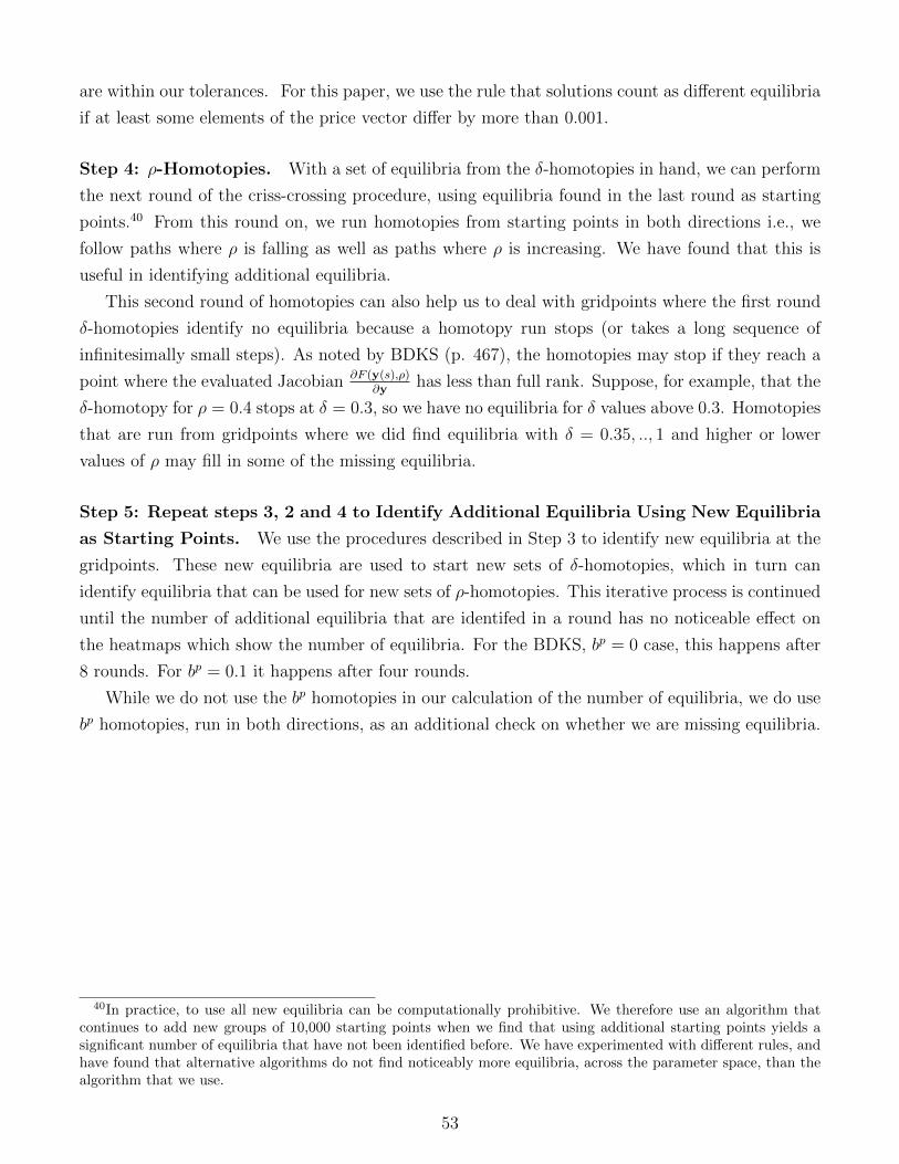
are within our tolerances. For this paper, we use the rule that solutions count as different equilibria
if at least some elements of the price vector differ by more than 0.001.
Step 4: ρ-Homotopies. With a set of equilibria from the δ-homotopies in hand, we can perform
the next round of the criss-crossing procedure, using equilibria found in the last round as starting
points.40 From this round on, we run homotopies from starting points in both directions i.e., we
follow paths where ρ is falling as well as paths where ρ is increasing. We have found that this is
useful in identifying additional equilibria.
This second round of homotopies can also help us to deal with gridpoints where the first round
δ-homotopies identify no equilibria because a homotopy run stops (or takes a long sequence of
infinitesimally small steps). As noted by BDKS (p. 467), the homotopies may stop if they reach a
point where the evaluated Jacobian ∂F (y(s),ρ)∂y
has less than full rank. Suppose, for example, that the
δ-homotopy for ρ = 0.4 stops at δ = 0.3, so we have no equilibria for δ values above 0.3. Homotopies
that are run from gridpoints where we did find equilibria with δ = 0.35, .., 1 and higher or lower
values of ρ may fill in some of the missing equilibria.
Step 5: Repeat steps 3, 2 and 4 to Identify Additional Equilibria Using New Equilibria
as Starting Points. We use the procedures described in Step 3 to identify new equilibria at the
gridpoints. These new equilibria are used to start new sets of δ-homotopies, which in turn can
identify equilibria that can be used for new sets of ρ-homotopies. This iterative process is continued
until the number of additional equilibria that are identifed in a round has no noticeable effect on
the heatmaps which show the number of equilibria. For the BDKS, bp = 0 case, this happens after
8 rounds. For bp = 0.1 it happens after four rounds.
While we do not use the bp homotopies in our calculation of the number of equilibria, we do use
bp homotopies, run in both directions, as an additional check on whether we are missing equilibria.
40In practice, to use all new equilibria can be computationally prohibitive. We therefore use an algorithm thatcontinues to add new groups of 10,000 starting points when we find that using additional starting points yields asignificant number of equilibria that have not been identified before. We have experimented with different rules, andhave found that alternative algorithms do not find noticeably more equilibria, across the parameter space, than thealgorithm that we use.
53

B Recursive Algorithms for Establishing Existence and
Uniqueness of Accommodative and SELPM Equilibria
in the BDK Model
Our second approach to finding equilibria in the BDK model uses backwards induction to exploit
the fact that two common types of equilibria have absorbing terminal states.
Definition An equilibrium is accommodative if λ1(e1, e2) = λ2(e1, e2) = 1 for all states e >
(0, 0).
In an accommodative equilibrium there is no exit by active firms. If the industry starts off in
state (1,1), it is guaranteed to arrive in state (M,M) in an accommodative equilibrium. This
definition is the same as in BDK (2019), Appendix B.
Definition An equilibrium has the“Some Exit Leads to Permanent Monopoly” (SELPM) property
if there is some e = (e1, e2) where e1 > e2 > 0, and (i) λ2(e) < 1, (ii) λ2(e′1, 0) = 0 and λ1(e
′1, 0) = 1
for all e′1 ≥ e1, and (iii) λ1(e′1, e′2) = 1 for all e′1 ≥ e1, e
′2 ≥ e2.
In a SELPM equilibrium, once the game has reached a state e that satisfies the requirements
the game will not return to that state once it has left it, and the game must eventually end up in
either state (M,M), state (M, 0) or state (0,M). Exit followed by entry can occur at earlier states.
B.1 Existence of an Accommodative Equilibrium
We establish whether an accommodative equilibrium exists by solving, using fsolve in MATLAB
with analytic derivatives, for equilibrium prices and values assuming that there is no exit from
any duopoly state, and then verifying that it is always optimal for each duopolist to continue by
checking that βV S(e1, e2) is greater than the highest possible scrap value for all e1, e2 > 0.
B.2 Existence of a SELPM Equilibrium and Uniqueness of Accom-modative Equilibria
We now describe how we identify whether a SELPM equilibria exists, before noting how we can
use a closely related procedure to check whether an accommodative equilibrium is unique. As we
explain, our conclusions that an accommodative equilibrium is unique or that no SELPM equilibria
exist rely on our ability to find all equilibria in a given state, holding fixed what will happen if and
when the state transitions. We explain why we are confident that we can do this.
B.2.1 Procedure for Establishing whether a SELPM Equilibrium Exists
Overview. We first solve for values and a monopolist firm 1’s strategies in states (1, 0) to (M, 0)
assuming that no entry will occur (we will later verify if this assumption is correct). We then use
54

backwards induction from state (M,M), where there will be a unique equilibrium with no exit (if
one exists), solving, in each state, for all equilibrium combinations of prices, values and the laggard’s
continuation probabilities that are consistent with the SELPM criteria, and checking whether in a
state (e1, 0) the potential entrant will not want to enter. As soon as we identify a state e which
satisfies the SELPM conditions (i.e., there is some probability of exit by the laggard, and if it occurs
there will never be re-entry) on an equilibrium path, we have established that a SELPM equilibria
exists (i.e., we do not need to find what strategies are in earlier states). We can, however, continue
to go back through the game to establish if an AELPM equilibrium (i.e., one where any exit leads
to permanent monopoly) exists.
We present our routine assuming that σ = 1 to reduce notation. Our examples assume the
baseline parameters ρ = 0.75 and σ = 1 unless otherwise stated.
Step 1: Solving for Outcomes with Permanent Monopoly. We solve for equilibria in states
with monopoly, (1, 0) to (M, 0), using backwards induction assuming that the monopolist and the
strategic buyers expect no entry by the potential entrant in these states. Note that while we solve
for this type of equilibrium in all monopoly states, this does not preclude the possibility that there
may, in a SELPM equilibrium, be re-entry in some of the monopoly states where the incumbent
has low know-how.
The equilibrium in state (M, 0) will be unique for all values of bp. With bp = 0 this follows from
the fact that, in state (M, 0) the game is simply a repeated monopoly pricing problem. However,
demand, and therefore the seller’s problem, is identical in this state for any value of bp, because the
strategic buyer cannot affect the evolution of the state, so the same conclusion holds.
Assuming that a monopolist will not exit (a condition that can be verified and is always satisfied
for the parameters that we consider), the equations that determine the equilibrium values of V B,
V S1 and p1 in state (e1 < M, 0), where firm 1’s marginal cost is c, are
V B = bp(ln(exp(βV B) + exp(v − p1 + βV B(e1 + 1, 0)
))+ ... (12)
β(1− bp)(D1VB(e1 + 1, 0) + (1−D1)V
B)
V S = (p1 − c+ βV S(e1 + 1, 0))D1 + βV S(1−D1) (13)
D1 + (p1 − c+ βV S(e1 + 1, 0)− βV S)∂D1
∂p1= 0 (14)
where D1 =exp(v−p1+βV B(e1+1,0))
exp(v−p1+βV B(e1+1,0))+exp(βV B)assuming, following BDK, that v0 = p0. V B and V S
denote V B(e1, 0) and V S(e1, 0) respectively. The last equation is the first-order condition for setting
prices. When we are solving for the equilibrium in state (e1, 0), V B(e1 + 1, 0) and V S(e1 + 1, 0) are
fixed.
We can check for evidence of multiplicity in states (e1 < M, 0) by identifying whether two
55
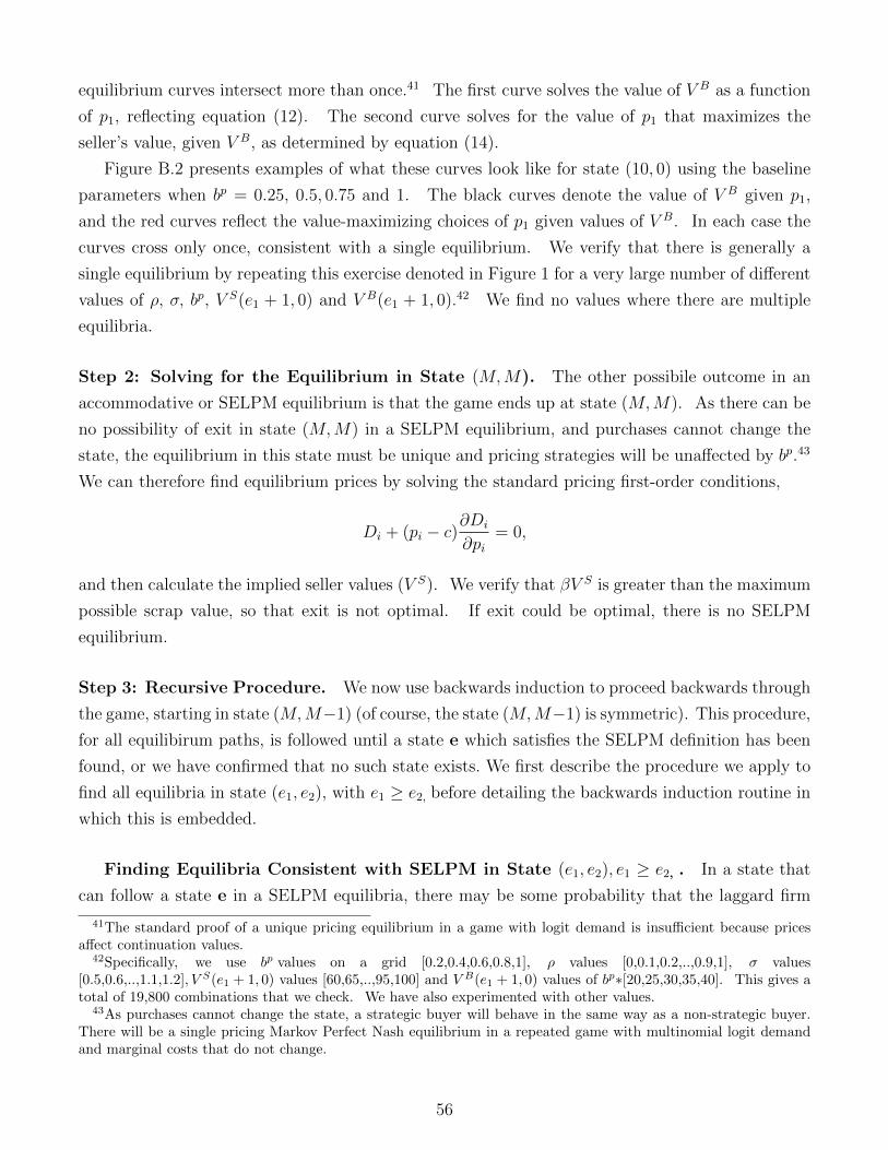
equilibrium curves intersect more than once.41 The first curve solves the value of V B as a function
of p1, reflecting equation (12). The second curve solves for the value of p1 that maximizes the
seller’s value, given V B, as determined by equation (14).
Figure B.2 presents examples of what these curves look like for state (10, 0) using the baseline
parameters when bp = 0.25, 0.5, 0.75 and 1. The black curves denote the value of V B given p1,
and the red curves reflect the value-maximizing choices of p1 given values of V B. In each case the
curves cross only once, consistent with a single equilibrium. We verify that there is generally a
single equilibrium by repeating this exercise denoted in Figure 1 for a very large number of different
values of ρ, σ, bp, V S(e1 + 1, 0) and V B(e1 + 1, 0).42 We find no values where there are multiple
equilibria.
Step 2: Solving for the Equilibrium in State (M,M). The other possibile outcome in an
accommodative or SELPM equilibrium is that the game ends up at state (M,M). As there can be
no possibility of exit in state (M,M) in a SELPM equilibrium, and purchases cannot change the
state, the equilibrium in this state must be unique and pricing strategies will be unaffected by bp.43
We can therefore find equilibrium prices by solving the standard pricing first-order conditions,
Di + (pi − c)∂Di
∂pi= 0,
and then calculate the implied seller values (V S). We verify that βV S is greater than the maximum
possible scrap value, so that exit is not optimal. If exit could be optimal, there is no SELPM
equilibrium.
Step 3: Recursive Procedure. We now use backwards induction to proceed backwards through
the game, starting in state (M,M−1) (of course, the state (M,M−1) is symmetric). This procedure,
for all equilibirum paths, is followed until a state e which satisfies the SELPM definition has been
found, or we have confirmed that no such state exists. We first describe the procedure we apply to
find all equilibria in state (e1, e2), with e1 ≥ e2, before detailing the backwards induction routine in
which this is embedded.
Finding Equilibria Consistent with SELPM in State (e1, e2), e1 ≥ e2, . In a state that
can follow a state e in a SELPM equilibria, there may be some probability that the laggard firm
41The standard proof of a unique pricing equilibrium in a game with logit demand is insufficient because pricesaffect continuation values.
42Specifically, we use bp values on a grid [0.2,0.4,0.6,0.8,1], ρ values [0,0.1,0.2,..,0.9,1], σ values[0.5,0.6,..,1.1,1.2], V S(e1 + 1, 0) values [60,65,..,95,100] and V B(e1 + 1, 0) values of bp∗[20,25,30,35,40]. This gives atotal of 19,800 combinations that we check. We have also experimented with other values.
43As purchases cannot change the state, a strategic buyer will behave in the same way as a non-strategic buyer.There will be a single pricing Markov Perfect Nash equilibrium in a repeated game with multinomial logit demandand marginal costs that do not change.
56
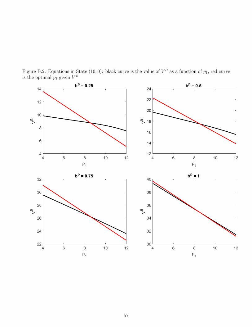
Figure B.2: Equations in State (10, 0): black curve is the value of V B as a function of p1, red curveis the optimal p1 given V B
57
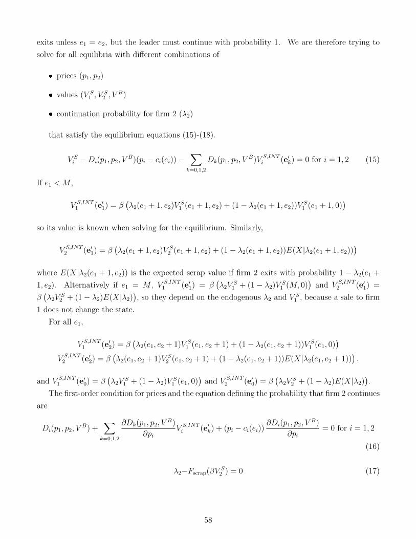
exits unless e1 = e2, but the leader must continue with probability 1. We are therefore trying to
solve for all equilibria with different combinations of
� prices (p1, p2)
� values (V S1 , V
S2 , V
B)
� continuation probability for firm 2 (λ2)
that satisfy the equilibrium equations (15)-(18).
V Si −Di(p1, p2, V
B)(pi − ci(ei))−∑
k=0,1,2
Dk(p1, p2, VB)V S,INT
i (e′k) = 0 for i = 1, 2 (15)
If e1 < M ,
V S,INT1 (e′1) = β
(λ2(e1 + 1, e2)V
S1 (e1 + 1, e2) + (1− λ2(e1 + 1, e2))V
S1 (e1 + 1, 0)
)so its value is known when solving for the equilibrium. Similarly,
V S,INT2 (e′1) = β
(λ2(e1 + 1, e2)V
S2 (e1 + 1, e2) + (1− λ2(e1 + 1, e2))E(X|λ2(e1 + 1, e2))
)where E(X|λ2(e1 + 1, e2)) is the expected scrap value if firm 2 exits with probability 1 − λ2(e1 +
1, e2). Alternatively if e1 = M , V S,INT1 (e′1) = β
(λ2V
S1 + (1− λ2)V S
1 (M, 0))
and V S,INT2 (e′1) =
β(λ2V
S2 + (1− λ2)E(X|λ2)
), so they depend on the endogenous λ2 and V S
1 , because a sale to firm
1 does not change the state.
For all e1,
V S,INT1 (e′2) = β
(λ2(e1, e2 + 1)V S
1 (e1, e2 + 1) + (1− λ2(e1, e2 + 1))V S1 (e1, 0)
)V S,INT2 (e′2) = β
(λ2(e1, e2 + 1)V S
2 (e1, e2 + 1) + (1− λ2(e1, e2 + 1))E(X|λ2(e1, e2 + 1))).
and V S,INT1 (e′0) = β
(λ2V
S1 + (1− λ2)V S
1 (e1, 0))
and V S,INT2 (e′0) = β
(λ2V
S2 + (1− λ2)E(X|λ2)
).
The first-order condition for prices and the equation defining the probability that firm 2 continues
are
Di(p1, p2, VB) +
∑k=0,1,2
∂Dk(p1, p2, VB)
∂piV S,INTi (e′k) + (pi − ci(ei))
∂Di(p1, p2, VB)
∂pi= 0 for i = 1, 2
(16)
λ2−Fscrap(βV S2 ) = 0 (17)
58

where
V B − bp log
( ∑k=0,1,2
exp(vk − pk + V B,INT (e′k)
))− (1− bp)
∑k=0,1,2
Dk(p1, p2, VB)V B,INT (e′k) = 0,
(18)
V B,INT (e′2) = β(λ2(e1, e2 + 1)V B(e1, e2 + 1) + (1− λ2(e1, e2 + 1))V B(e1, 0)
), (19)
V B,INT (e′0) = β(λ2V
B + (1− λ2)V B(e1, 0)), (20)
and
V B,INT (e′1) = β(λ2(e1 + 1, e2)V
B(e1 + 1, e2) + (1− λ2(e1 + 1, e2))VB(e1 + 1, 0)
)(21)
if e1 < M , and
V B,INT (e′1) = β(λ2V
B + (1− λ2)V B2 (e1, 0)
)(22)
if e1 = M .
There can be multiple solutions to these equations. We proceed assuming that there is a single
equilibrium for a given value of λ2, an assumption that we will verify below, and solve equations
(15), (16) and (18) given this value.44 Given the prices and values, we then calculate what the
optimal exit probability will be using (17). When we use a fine grid of values of λ2 we can construct
graphs like the ones shown in Figure B.3, which show this best response λ2 function, as a function of
an arbitrary λ2, for the baseline parameters, for states (30,1) and (30,5), with bp = 0 and bp = 0.2.
There is an equilibrium where the function crosses the 450 line, and we identify the precise
solutions to all of the equations using the solutions at the gridpoints that surround the intersection
as starting points. We then verify whether or not the leader wants to continue with probability 1,
which is necessary for a SELPM equilibrium. Assuming that our initial grid of λ2 is sufficiently
fine, this approach will find all of the equilibria in a given state that are consistent with the SELPM
criteria.
Backward Induction Algorithm. Our aim is to identify whether a SELPM equilibrium
exists. Therefore we follow equilibrium paths through the state space until we can identify a state
which satisfies all of the requirements for a state e in the definition of a SELPM equilibrium, at
which point the algorithm terminates in success, or, alternatively, we have followed all equilibrium
paths and found that there is no such state, because along each path it is case that either a leader
may choose to exit, no exit occurs anywhere in the game or there is positive probability that re-entry
may occur after any exit. In this alternative case, no SELPM equilibrium exists.
The order in which we loop through states is to go from e1 = 30 to e1 = 1 as the outer loop, and
to go from e2 = e1 to e2 = 1 on the inner loop, while performing an additional check on whether
re-entry may be optimal if e2 = 0.
44Occasionally the equations do not solve using the starting values chosen, in which case we use a Pakes-McGuiretype of routine to find alternative starting values.
59

Figure B.3: Best Response Continuation Probability Functions for Firm 2: cases where the blackand red lines cross the 450-degree line represent equilibria
As an example, consider the baseline parameters. With bp = 0, the backwards induction
algorithm identifies a single equilibrium path with no exit until state (30, 1) where it identifies three
equilibria with probabilities that firm 2 continues (λ2) of 0.7777, 0.9577 and 1 (these correspond to
the three intersections of the black line and the 450 line in the second panel of Figure B.3). If we
take the first equilibrium, we can identify that it is never optimal for firm 2 to enter in state (30, 0).
This implies that (30, 1) is a state that meets the criteria for a state e in a SELPM equilibria, so
the algorithm terminates at this point. We would reach the same conclusion using the second
equilibrium. On the other hand, when bp = 0.2 we identify only a single equilibrium path where
there is no exit in any state all of the way back to (1, 1). In this case, we can conclude that no
SELPM equilibrium exists.
Verifying the Uniqueness of Equilibrium in a State Given a Firm 2 Continuation
Probability. The conclusion that there is no SELPM equilibrium for given parameters relies on
us having identified all equilibrium paths that could meet the SELPM criteria. This will be the
case as long as there cannot be multiple price equilibria for a given probability that the laggard
firm continues.
60

There are two types of evidence that support this presumption. First, we have never identified
an instance of multiple equilibria for any of the parameters that we have considered, even when
using multiple different starting points or alternative solution algorithms. Second, we have tried
to identify whether there could be multiple equilibria by using a reaction function-type of analysis.
Specifically, for a given value of λ2 and the continuation values, we solve the equations for V B,
V S1 and the first-order condition for p1 for a grid of alternative values of p2. We then solve the
equations for V B, V S2 and the first-order condition for p2 for a grid of alternative values of p1. We
can then draw curves p∗1(p2) and p∗2(p1), which reflect the best response behavior of strategic buyers
to both prices. The intersections correspond to equilibria, and we can test whether they intersect
more than once. Figures B.4 present some examples of these curves for the baseline parameters,
bp = 0 or bp = 1 and e1 = 30 and e2 = 1.
Recall that in the state (30,1), if the buyer purchases from firm 1, the state remains (30,1),
whereas is firm 2 makes a sale the state transitions to (30,2), where for these parameters there is
always a unique equilibrium. If firm 2 sets a very low price, a strategic buyer will tend to shift
demand towards firm 1 in order to keep the state the same in future periods. As a result, firm
1’s optimal price is less sensitive to firm 2’s price in this state when bp = 1, which accounts for
the change in the slope of the reaction functions. However, in all cases, the reaction functions only
intersect once, and there is a single equilibrium.
In practice, it would be too computationally intensive to implement this check for every value
of λ2 in every state. However, for all of the values of the parameters where our algorithm does
not identify a SELPM equilibrium, but it does for nearby parameter values, we have performed
the check for a grid of values of λ2. In each case, we have identified exactly one intersection
(equilibrium) and are therefore confident in our claim that we are not missing SELPM equilibria.
This is also the case when we have solved games for many different sets of arbitrary continuation
values and parameters.
B.2.2 Procedure for Identifying the Existence of AELPM Equilibria
Definition An equilibrium has the“Any Exit Leads to Permanent Monopoly” (AELPM) property
if (i) for any e = (e1, e2) where e1 > e2 > 0, and λ2(e) < 1, λ2(e′1, 0) = 0 for all e′1 ≥ e1;(ii)
λ1(e, e) = 1 for all e > 0, and (iii) λ1(e1, e2) = 1 for all e1 > e2.
In an AELPM equilibrium, any exit by a laggard firm in duopoly will lead to permanent
monopoly. We can establish whether an AELPM equilibrium exists using a similar equilibrium
path following procedure to the one used for SELPM equilibria, except that we now need to follow
paths from (30, 30) to (1, 1) to make sure that no exit is followed by re-entry, and that symmetric
firms will never exit.
For the baseline parameters with bp = 0, the equilibrium path that contains λ2(30, 1) = 0.9577
does find an AELPM equilibrium (which corresponds to the mid-HHI equilibrium in Table 1). On
61

Figure B.4: Pricing Best Response Functions in State (30,1) for Different Continuation Probabilitiesfor Firm 2 (λ2)
(a) bp = 0
(b) bp = 1
62

the other hand, the equilibrium path that contains λ2(30, 1) = 0.7777 fails the AELPM test when
it reaches (1,1) as, in the corresponding high-HHI equilibrium, there is a small probability that one
of the firms will exit.
The computational burden involved in identifying whether AELPM equilibria exist is much
higher than the one that identifies if SELPM equilibria exist, because of the need to follow a path
all of the way through the state space and the possibility that there are a large number of paths,
all of which fail when both firms have low-levels of know-how. Therefore, we focus on the SELPM
results, and discuss AELPM equilibria in the context of classifying the equilibria identified by the
homotopy approach.
B.2.3 Establishing the Uniqueness of Accommodative Equilibria
Our evidence that accommodative equilibria are unique comes from the applying the procedure
described in the “Verifying the Uniqueness of Equilibrium in a State Given a Firm 2 Continuation
Probability” subsection, but considering only λ2 = 1. We have not found more than one intersection
(equilibrium) in more than one state for any set of parameters.
C Additional Results
C.1 bp-Homotopies Illustrating the Results for the Number of Equilib-ria in the BDKS Model
The main results from the analysis of the number of equilibria in the BDKS model are that (i) the
number of equilibria typically declines quite quickly as bp is increased, so that, when bp ≥ 0.1 there
is typically a unique equilibrium, but (ii) there are some parameters where the number of equilibria
increases when we move from bp = 0 to bp = 0.05. These results are based on δ- and ρ-homotopies,
so in this Appendix sub-section we illustrate that the results are consistent with what one finds
using bp-homotopies. While we only present results for two parameters, we see similar results for
many other parameters that we have looked at.
Figure C.2(a) shows an example where there are seven equilibria identified by the δ- and ρ-
homotopies when bp = 0. When we start the bp-homotopies from each of these equilibria we
find that there are 3 pairs that are connected by semi-circular loops, none of which extend past
bp = 0.03 and, from the equilibrium with the lowest concentration, a fairly flat path (with respect
to the concentration outcome) that continues through higher values of bp.
Figure C.2(b) shows an example where there is a single equilibrium identified by the δ- and
ρ-homotopies when bp = 0. The bp-homotopy from this equilibrium forms a loop, but, when it
reaches a value of bp just above 0.01 it reverses itself and then continues out through higher values
of bp. In this case we find multiplicity of equilibria only for bp = 0.05 out of the discrete values we
consider.
63

Figure C.2: Extended BDKS Mode: Examples of bp-Homotopies From bp = 0 Equilibria
(a) δ = 0.066, ρ = 0.31
(b) δ = 0.028, ρ = 0.85
64

C.2 Outcomes in the Extended BDKS Model as a Function of bp forδ = 0.0275 and ρ = 0.85 and bp = 0 Seller Strategies
In the text we report what happens to a set of outcomes when we hold seller strategies fixed and
increase bp for the parameters δ = 0.0275 and ρ = 0.75. We choose ρ = 0.75 so that learning
effects are the same as in the baseline example that we use in analyzing the BDK model. However,
BDKS use values δ = 0.0275 and ρ = 0.85 so we report these comparisons in this Appendix. Like
BDKS, we identify two equilibria for these parameters, and rather than the “diagonal trench” and
“sideways trench” equilibria that we find for δ = 0.0275 and ρ = 0.75, in this case the equilibria
can be described as having a diagonal trench and “flat with well” (where there are low prices in
state (1,1), but otherwise there is no obvious dip).
Figure C.3 are similar to those reported in the text, with the most obvious differences arising
from the fact that buyer choices are less sensitive to bp in the flat with well equilibrium than the
sideways trench equilibrium. This makes sense as buying from the laggard in state (3,1) immediately
puts the game into the sideways trench where prices are particularly low, whereas buying from the
laggard, and pushing the market towards symmetry, has milder effects in the flat with well case. The
advantage denying incentives are also somewhat smaller, although the advantage-denying incentives
retain a non-monotonic pattern.
65

Figure C.3: Extended BDKS Model: Outcomes as a Function of bp for δ = 0.0275 and ρ = 0.85and bp = 0 Seller Strategies.
(a) Inverse Demand Curves For Seller 1 in State (3,1)
(b) Distribution of States after 10 Periods for δ = 0.0275 and ρ = 0.85 and bp = 0 Seller Strategies. Therange of the duopoly state indicates the difference in the states of the two active firms, so that, for example,(e1 = 7, e2 = 2) would be in the Duopoly: 4-5 category.
66

Figure C.3: Extended BDKS Model: Outcomes as a Function of bpfor δ = 0.0275 and ρ = 0.85 andbp = 0 Seller Strategies.
(c) Firm 1 Advantage-Building and Advantage-Denying Incentives in State (3,1): F =Flat with Well, DT= Diagonal Trench
67

C.3 Extended BDKS Model: ρ-Homotopies with δ = 0.05
Figures C.4 and C.5 show how expected long-run market concentration and average prices, and the
NPV of consumer and total surplus, for a game starting at (1,1), vary with ρ and bp, holding δ fixed
at 0.05. The figures should be read with ρ = 1, at the left edge, corresponding to no LBD, with
faster and more dramatic cost reductions from LBD as one moves to the right. δ = 0.05 corresponds
to a forgetting probability of 0.54 for ei = 15, so, in expectation, it is not quite possible to sustain
two firms at the bottom of their cost curves.
Consistent our results for the number of equilibria, there is multiplicity for low bp for high and
low values of ρ, but these are eliminated as bp rises, so that there is a unique equilibrium for all ρ for
bp ≥ 0.1. Consistent with the rest of our analyses, expected long-run concentration tends to be lower
with higher bp, and when bp = 1 the firms are expected to be close to symmetric in the long-run
even though there will be a continuous process where the firms gain and lose (forget) know-how.
Concentration also tends to be low for very high and low ρ as, in both cases, marginal costs are close
to their minimum possible values for low levels of know-how so that, even with forgetting, both
firms firms can be expected to be close to the bottom of their cost curves, whereas for intermediate
values of ρ only a firm that gains an advantage over its rival may be able to maintain low costs.
Figure C.4(b), which reports differences in prices from those when bp = 1, shows that when ρ
lies between 0.4 and 0.8 long-run prices are significantly higher when bp is very low, reflecting the
fact that the market is dominated by a single firm. On the other hand, for bp ≥ 0.1 the effect that
increasing bp tends to soften competition dominates and prices increase. For more extreme values
of ρ, where there can be multiple equilibria for low bp, the prices in some equilibria are lower than
those in the unique equilibrium when buyers are more strategic, and prices in other equilibria are
lower.
Figure C.5 compare the NPV of total and consumer surplus as a function of ρ for different levels
of bp. In general, the differences in surplus across different values of bp (they are measured relative
to the unique outcome when bp = 1) are small, but they indicate that even when more aggressive
pricing results in more concentrated outcomes and higher long-run prices, the lower initial prices
may raise the NPV of surplus.45 Similar to a pattern in the BDK model (see Section 4.2), for very
high ρ, strategic buyer behavior can actually slightly increase total surplus as they internalize how
purchases can lower costs over a number of periods.
45As sales are always made in the BDKS model, the increase in total surplus reflects the reduction in productioncosts that comes from most sales being made by the lower-cost leader.
68

Figure C.4: Extended BDKS Model: Long-Run Expected HHI and Average Prices with δ = 0.05
(a) Expected Long-Run HHI (HHI∞)
(b) Expected Long-Run Prices (Relative to Unique Outcome Where bp = 1)
69

Figure C.5: Extended BDKS Model: NPV of Welfare with δ = 0.05. Measured Relative to theUnique Outcome Where bp = 1.
(a) Consumer Surplus
(b) Total Surplus
70
Top Related