Dynamic Cointegrated Pairs Trading:Time-Consistent Mean-Variance Strategies

Mei Choi Chiu and Hoi Ying Wong∗

Department of StatisticsThe Chinese University of Hong Kong

September 3, 2012

Abstract

Cointegration is a useful econometric tool for identifyingassets whichshare a common equilibrium. Cointegrated pairs trading is atrading strategywhich attempts to take a profit when cointegrated assets depart from theirequilibrium. This paper investigates the optimal dynamic trading of cointe-grated assets using the classical mean-variance portfolioselection criterion.To ensure rational economic decisions, the optimal strategy is obtained overthe set of time-consistent policies from which the optimization problem isenforced to obey the dynamic programming principle. We solve the opti-mal dynamic trading strategy in a closed-form explicit solution. This ana-lytical tractability enables us to prove rigorously that cointegration ensuresthe existence of statistical arbitrage using a dynamic time-consistent mean-variance strategy. This provides the theoretical grounds for the market beliefin cointegrated pairs trading. Comparison between time-consistent and pre-commitment trading strategies for cointegrated assets shows the former tobe a persistent approach, whereas the latter makes it possible to generateinfinite leverage once a cointegrating factor of the assets has a high meanreversion rate.

Keywords: Cointegration; Mean-Variance Portfolio Theory; Pair Trade; Time-consistency.

∗Corresponding author; E-mail:hywong@cuhk.edu.hk

1

1 Introduction

The concept of cointegration, which led to Nobel prize-winning work in 2003,originated with Granger (1981) and Engle and Granger’s (1987) assertion that alinear combination of non-stationary economic series could be stationary, thussignifying the co-movement of economic series beyond the conventional corre-lation coefficient. Cointegration techniques have been applied to examining theco-movement of a variety of financial assets, including stocks (Cerchi and Haven-ner, 1988; Taylor and Tonks, 1989; Mylonidis and Kollias, 2010), exchange rates(Baillie and Bollerslev, 1989; Kellard et al., 2010) and commodities (Maslyukaand Smyth, 2009). They have also brought new insights into hedging (Alexander,1999) and index tracking (Alexander and Dimitriu, 2005).

Cointegration is also an important tool in pairs trading (Vidyamurthy, 2004).As cointegrated stocks should theoretically have a narrow spread in long-termequilibrium, a hedge fund strategy is to bet on the spread by long-short or relative-value arbitrage. If the spread widens, then the strategy is to short the high stockand buy the low stock. As the spread narrows to some equilibrium value, un-winding the position results in a profit. Practitioners usedto specify a threshold,which, when exceeded by the spread, would trigger a trade. The optimal choiceof threshold, the amounts invested in the long and short positions, and the lengthof holding time are rules of thumb in practice. This relative-value arbitrage is,however, a suboptimal strategy. When two cointegrated stocks are undervaluedrelative to their long-term means, it could be better to longboth rather than bettingon their spread. Gatev et al. (2006) show that this simple relative-value arbitragegenerates profits, but the contribution of mean reversion (or cointegration) is notsignificant. In addition, relative-value arbitrage is a static strategy that does nottake advantage of dynamic trading.

The dynamic trading of cointegrated assets is an interesting topic in finance.Wachter (2002) considers the dynamic trading of a mean-reverting risky asset, aspecial case of cointegration, and a risk-free bond in a complete market. Jurekand Yang (2007) attempt to solve the dynamic trading of cointegrated assets us-ing the utility function with constant risk aversion. Although they successfullysolve the problem for the case of a single mean-reverting risky asset and a risk-free bond, their solution can be generalized only touncorrelated cointegrated as-sets. Using the Markowitz (1952) mean-variance (MV) criterion, Chiu and Wong(2011) systematically investigate the optimal dynamic trading strategy of cointe-grated assets with a general correlation structure. The latter’s solution, however,is a time-inconsistent (or precommitment) policy, which violates the dynamic pro-

2

gramming principle of optimization. Such an obstacle is shared by most relatedwork, such as that of Li and Ng (2000), Zhou and Li (2000), Bielecki et al. (2005),and many others due to the subtle non-separability of the MV objectives.

Investigation of time-consistent dynamic MV asset allocation has recently at-tracted a great deal of attention in the literature. In a discrete-time setting forexample, Cui et al. (2010) show that it is possible to construct a trading strategythat always outperforms the optimal MV precommitment policy by taking advan-tage of time-inconsistency. In a continuous-time economy,Basak and Chabakauri(2010) propose a framework for deriving time-consistent optimal MV portfoliopolicies and apply it to the wealth allocation between a risky stock and a risk-free bond. Bjork et al. (2011) generalize their work to allowstate-dependentrisk aversion. Wang and Forsyth (2011) construct numericalschemes for theHamilton-Jacobi-Bellman (HJB) equations associated withtime-consistent MVportfolio problems subject to different market constraints.

In this paper, we investigate the dynamic trading of cointegrated assets andoffer an optimal time-consistent asset allocation policy based on the MV crite-rion. The dynamics of the assets are the diffusion limit of the discrete-time error-correction model of cointegrated time series derived by Duan and Pliska (2004).Using the framework developed by Basak and Chabakauri (2010), time-consistentdynamic cointegrated pairs trading strategies are systematically derived in explicitand closed-form solutions.

In addition to its mathematical derivations, this paper contributes to the financeliterature by providing insights into several important questions. For example, isthere any relationship between cointegration and statistical arbitrage? Using thedefinition of statistical arbitrage in Hogan et al. (2004), we rigorously prove thatthe existence of cointegration ensures the existence of a statistical arbitrage strat-egy. In particular, an optimal time-consistent MV portfolio policy with an infiniteinvestment time is precisely such a strategy. In a financial market in which non-stationary economic series cannot be error-corrected, time-consistent MV policiesfail to deliver statistical arbitrage profits and are asymptotically no-arbitrage. Inthe Black-Scholes market, in which, the log-values of riskyassets follow Brow-nian motions, statistical arbitrage asymptotically exists, but the long-term time-consistent MV policy suggests no investment.

Whereas the statistical arbitrage concept considered in Hogan et al. (2004)concerns long-term investments, practitioners are more concerned with finite-time, particularly short-term, investments. Does cointegration enhance profitabil-ity in finite time? By defining profitability as the trade-off between risk and return,our theory predicts that the time-consistent MV trading of cointegrated risky assets

3

generates a higher price of risk or Sharpe ratio than that of risky assets followingthe Black-Scholes model. We develop an index to measure the profitability ofdifferent cointegrated pairs.

As the relative-value arbitrage rule is a popular trading strategy, it is naturalto ask whether our optimal trading strategy resembles a long-short trading rule.We provide a counter example that illustrates numerically acase of short-sellinga pair of cointegrated assets for a risk-free bond. Such a situation occurs whenthe two assets are overvalued. Unlike the relative-value arbitrage rule reported inGatev et al. (2006), the mean reversion rate contributes significantly to the profitof dynamic pairs trading with the MV objective.

What is the major advantage of the time-consistent policy over the precom-mitment policy? Basak and Chabakauri (2010) find that, in general, the time-consistent policy suggests less investment in risky assetsthan its precommitmentcounterpart, thus implying that the former is more prudent.Their game-theoreticargument further justifies the economic soundness of time-consistent MV policies.Using the Black-Scholes model of risky assets, Wang and Forsyth (2011) show nu-merically that the price of risk from the precommitment policy is greater than thatfrom the time-consistent policy. We supplement their results by demonstratingthat the precommitment policy for cointegrated assets suffers from the problem ofa finite escape time at which investors are recommended to take infinite positions.Time-consistent policies do not share this problem. This shortcoming of the pre-commitment policy implies the inadequate robustness of theoptimal trading ruleto the estimated model parameters. The time-consistent policy, in contrast, is morerobust, particularly to the mean reversion rate. The time-consistent constraint im-posed on the portfolio problem confines us to rational decisions, which do not takefull advantage of the assumed stochastic model, but render it more stable.

The rest of this paper is organized as follows. Section 2 introduces the coin-tegration dynamics and details the problem formulation. The time-consistent MVportfolio problem is completely solved in Section 3. The optimal policy and effi-cient frontier for trading cointegrated assets are derivedin closed-form solutions.The analytical results are then applied to the pairs tradingof cointegrated assetsin Section 4. In particular, we investigate the arbitrage ofdynamic cointegratedpairs trading using the MV portfolio theory. The derived time-consistent policyis contrasted with its precommitment policy. Numerical examples are provided toillustrate the application. Section 5 concludes the paper.

4

2 Problem formulation

2.1 Cointegration

Granger’s representation theorem enables the cointegrated vector time series tobe expressed as an error correction model. In discrete time,an error correctiondynamic for then-component asset price time series withk (1 ≤ k ≤ n) cointe-grating factors is defined as follows.

ln Si,t − ln Si,t−1 = µi +k∑

j=1

δijzj,t−1 + σi,tǫi,t, i = 1, . . . , n,

zj,t = aj + bjt +

n∑

i=1

cij ln Si,t for j = 1, . . . , k,

whereSi,t is the price of risky asseti at timet for i = 1, . . . , n; (c1j , . . . , cnj)are linearly independent vectors forj = 1, . . . , k; σi,t is the volatility of asseti at time t; and the random vector[ǫ1,t, · · · , ǫn,t] follows a multivariate normaldistribution with mean zero and a constant correlation coefficient matrix. In theerror correction model, the vector ofk cointegrating factors,[z1,t, · · · , zk,t], formsa weakly stationary time series such that eachzj,t has a bounded variance at alltime points for allj = 1, 2, . . . , k.

Our analysis is based on the diffusion limit of the discrete-time error correctionmodel. Duan and Pliska (2004) derived the diffusion limit as

d lnSi,t =

(µi +

k∑

j=1

δijzj,t

)dt + σidWi,t, i = 1, . . . , n, (1)

zj,t = aj + bjt +

n∑

i=1

cij ln Si,t j = 1, . . . , k, (2)

whereWi,t are correlated Wiener processes.

2.2 The market

Using the concept of cointegration, we consider a financial market that containsn + 1 assets that are traded continuously within the time horizon[0, T ]. These

5

assets are labeled bySi for i = 0, 1, 2 . . . , n, with the0-th asset being risk-free.The risk-free asset satisfies the following differential equation.

dS0(t) = r(t)S0(t)dt,

S0(0) = R0 > 0,

wherer(t) is the time deterministic risk-free rate. The risky assets are definedthrough their log-price processes,X1(t), . . . , Xn(t), whereXj(t) = ln Sj(t). Bysubstituting (2) into (1), the vector of the log-prices of risky assets,X(t), satisfiesthe stochastic differential equation (SDE),

dX(t) = [θ(t) −AX(t)] dt + σ(t)dWt, t ∈ [0, T ], (3)

whereWt = (W 1t , . . . , W n

t )′ is a standardFt-adaptedn-dimensional Wiener pro-cess on a fixed filtered complete probability space(Ω,F ,P,Ft); W i

t andW jt are

mutually independent for alli 6= j; A is ann×n constant matrix of cointegrationcoefficients; andσ(t)σ(t)′ = Σ(t) is the covariance matrix of anRn×n-valuedcontinuous function on[0, T ]. Therefore, risky assets are correlated with a time-varying covariance matrix in general. In line with the literature, we assume thatthe non-degeneracy condition ofΣ(t) ≥ δIn holds for allt ∈ [0, T ] and for someδ > 0, whereasθ(t) andσ(t) are continuous functions on[0, T ].

SDE (3) represents the diffusion limit of the first-order vector autoregressive(VAR(1)) model with Gaussian innovations. The error correction model is a spe-cial VAR model that requires all eigenvalues ofA to be nonnegative real numbers(or complex numbers with nonnegative real parts). For the time being, we im-pose no condition on the matrixA to permit a general discussion. The concept ofcointegration will be useful in our analysis of statisticalarbitrage.

2.3 Mean-variance portfolio problem

Consider a mean-variance investor with an initial wealth ofY0 in the specifiedfinancial market with cointegration. The investor seeks an admissible portfoliostrategy so that the variance of the terminal wealth level isminimized and theexpected final wealth equalsY . Let ui(t) be the amount invested in asseti andNi(t) be the number of thei-th asset in the portfolio of the investor. The wealthof the investor at timet is then given byY (t) =

∑ni=0 ui(t) =

∑ni=0 Ni(t)Si(t).

The portfoliou(t) = (u1(t), u2(t), . . . , un(t))

′

6

is said to be admissible ifu(t) is a non-anticipating andFt-adapted process suchthat ∫ T

0

|u(τ)|2dτ < ∞ a.s.

In such a situation, we writeu ∈ L2FT

([0, T ], Rn).Applying Ito’s lemma toY (t) with respect to the cointegrating dynamics (3),

the wealth process is given by

dY (t) = [r(t)Y (t) + u(t)′α(t)] dt + u(t)′σ(t)dWt, (4)

Y (0) = Y0,

where1 is the column vector with all elements being 1, and

α(t) = θ(t) −AX(t) +1

2D(Σ(t))1 − r(t)1, (5)

in whichD(Σ(t)) is the diagonal matrix with all diagonal elements equal to thoseof the covariance matrixΣ(t) = σ(t)σ(t)′. Note thatα(t) is a random variableas it depends onX(t) through (5). Therefore, our portfolio optimization probleminvolves a random parameter in the wealth process which complicates the solutionderivation procedure.

Finding an optimal controlu(·) with respect to a certain objective function isreferred to as a portfolio selection problem in finance. The MV portfolio selectionproblem with cointegration is formulated as

P(MV)′ : minu

Var(Y (T ))

s.t. E[Y (T )] = Y , u ∈ L2FT

([0, T ], Rn), (4),

for a pre-specified expected final wealthY . A classical approach invokes theequivalent Lagrangian problem:

P(λ)′ : minu

Var(Y (T )) − 2λE[Y (T )]

s.t. u ∈ L2FT

([0, T ], Rn), (4).

After solving P(λ)′ for any givenλ > 0, the solution of P(MV)′ can be retrievedby matchingY with a suitable value ofλ.

Problems P(MV)′ and P(λ)′ have been systematically solved by Chiu andWong (2011). However, the generic spaceL2

FT([0, T ], Rn) of all possible asset

7

allocation policies does not guarantee that the solution follows the dynamic pro-gramming principle, which is a basic requirement of rational economic decisions(Strotz, 1956). In fact, Chiu and Wong (2011) obtained a precommitment policy.

For any givenλ > 0, consider the utility function1

Ut = Var(Y (T )| Ft) − 2λE[Y (T )| Ft].

Using the law of iterated expectations, Basak and Chabakauri (2010) show that aportfolio policy satisfying

Ut = E [Ut+τ | Ft] + Var(E[Y (T )| Ft+τ ]| Ft) , t ≥ 0, τ > 0 (6)

is a time-consistent policy that obeys the dynamic programming principle. Hence,we define the time-consistent solution space of the cointegrated assets as

U(t, T ) =u ∈ L2

FT([t, T ], Rn) : (4) and(6) hold

. (7)

The time-consistent versions of P(MV)′ and P(λ)′ are respectively revised as

P(MV) : minu∈U(0,T )

Var(Y (T )) s.t. E[Y (T )] = Y

and

P(λ) : minu∈U(0,T )

Var(Y (T )) − 2λE[Y (T )].

3 The trading strategy and efficient frontier

3.1 Time-consistent recursive equation

To solve problem P(λ), we need a time-consistent HJB equation for the valuefunction,

J(t, Y (t), X(t), T ) = minu∈U(t,T )

Var(Y (T )|Ft) − 2λE[Y (T )|Ft]. (8)

We denoteJ∗ := J(0, Y0, X(0), T ) as the initial value of the objective function inP(λ) with the optimal policy adopted.

1We use an alternative, but equivalent, utility function to Basak and Chabakauri (2010).

8

Using (4), an application of Ito’s lemma shows that

d(e∫ T

tr(s)dsY (t)

)= e

∫ T

tr(s)ds [α(t)′u(t)dt + u(t)′σ(t)dWt] , (9)

which implies

E[Y (T )|Ft] = e∫ T

tr(s)dsY (t) + E

[∫ T

t

e∫ T

sr(τ)dτα(s)′u(s)ds

∣∣∣∣Ft

], (10)

Var(Y (T )|Ft) = Var

(∫ T

t

e∫ T

sr(τ)dτα(s)′u(s)ds

+

∫ T

t

e∫ T

sr(τ)dτu(s)′σ(s)dWs

∣∣∣∣Ft

). (11)

Substituting (10) and (11) into (8) results in

J(t, Y (t), X(t), T ) = J1(t, X, T ) − 2λe∫ T

tr(s)dsY (t), (12)

where

J1(t, X, T ) = minu∈U(t,T )

Var(Y (T )|Ft) − 2λE

[∫ T

t

e∫ T

sr(τ)dτα(s)′u(s)ds

∣∣∣∣Ft

]. (13)

An interpretation of (12) is that the current wealth level,Y (t), is linearly separatedfrom the objective function. In other words, the optimal solution of P(λ), u∗(t, T ),does not depend on the wealth level at timet as it suffices to operate the dynamicprogramming on the functionJ1 which is independent ofY (t); see (11). Theaim of includingT in the optimal solution is to highlight its dependence on theinvestment period specified by the investor. The Markovian nature of the economyfurther ensures that the optimal policy depends solely onX(t) andt for any givenconstantλ. Hence, from now on, we designate the optimal policy asu∗(t, X, T ).

Lemma 3.1. The value functionJ(t, Y (t), X(t), T ) defined in (8) satisfies thefollowing HJB equation.

minu(t)

E[dJ |Ft] + Var(d(e

∫ T

tr(s)dsY ) + dΓ|Ft)

= 0, (14)

where

Γ(t, X(t), T ) = E

[∫ T

t

e∫ T

sr(τ)dτα(s)′u∗(s)ds|Ft

], (15)

u∗(t, X(t), T ) = e−∫ T

tr(s)ds

[λΣ(t)−1α(t) −

∂Γ

∂X(t, X(t))

], (16)

9

α(t) is defined in (5), and∂∂X

is the gradient operator with respect to the vector oflog-asset values,X. Further,u∗ in (16) is the optimal dynamic policy of P(λ).

Although Lemma 3.1 is a multivariate generalization of Basak and Chabakauri’s(2010) result, we do not regard it as an important contribution. The proof based ontheir approach is given in the appendix solely to produce a self-contained article.However, the major difficulty of our problem is the derivation of Γ in (15) andu∗

in (16) in explicit closed-form solutions in a financial market with cointegratedassets. The key to deriving these solutions is the recognition of a quadratic form.

3.2 The optimal trading strategy

Lemma 3.2. The functionΓ(t, X(t)) defined in (15) takes the form

Γ(t, X(t), T ) = λH(t, α(t), T ), (17)

whereα(t) is defined in (5), and

H(t, α(t), T ) = E[∫ T

tα(s)′Σ(s)−1α(s)ds

∣∣∣Ft

], (18)

which uses the equivalent probability measureP :

dP

dP= exp

∫ T

t

−1

2α(s)′Σ(s)−1α(s)ds −

∫ T

t

α(s)′Σ(s)−1σ(s)dWs

.

Proof. By substituting (16) into (15), we arrive at

Γ = E

[∫ T

t

(λα′Σ−1α −

(∂Γ

∂X

)′

α

)ds

∣∣∣∣Ft

]. (19)

Alternatively, applying Ito’s lemma toΓ(t, X) with respect toX yields

−Γ = E

[∫ T

t

(∂Γ

∂t+

(∂Γ

∂X

)′

(θ −AX) +1

2tr

(σ′ ∂

2Γ

∂X2 σ

))ds

∣∣∣∣Ft

], (20)

in which we use the fact thatΓ(T, X) = 0. Note that ∂∂X

is the gradient opera-tor with respect toX, ∂2

∂X2 the Hessian matrix operator, andtr(·) the trace of a

10

square matrix. Putting (19) and (20) together, we end up witha partial differentialequation (PDE) ofΓ:

∂Γ

∂t+

(∂Γ

∂X

)′

(θ −AX − α) +1

2tr

(σ′ ∂

2Γ

∂X2 σ

)+ λα′Σ−1α = 0, (21)

Γ(T, X, T ) = 0.

As the coefficient of the gradient vector and the drift ofX underP are differedby a vectorα, the result follows by the Feynman-Kac formula and the Girsanovtheorem.

Proposition 3.1. The time-consistent dynamically optimal trading strategyofproblem P(λ) is given by

u∗(t, X(t), T ) = λe−∫ T

tr(s)ds

[(Σ(t)−1 + A′K(t, T )

)α(t) + A′N(t, T )

], (22)

and the auxiliary functionH appearing in Lemma 3.2 is

H(t, α, T ) =1

2α′K(t, T )α + N(t, T )′α + M(t, T ), (23)

whereα(t) is defined in (5),D = D(Σ(t)),

K(t, T ) = 2

∫ T

t

Σ(s)−1ds ∈ Rn×n; (24)

N(t, T )′ =

∫ T

t

Θ(s)′K(s)ds ∈ R1×n; (25)

M(t, T ) =

∫ T

t

[N(s)′Θ(s) +

1

2tr(σ(s)′A′K(s)Aσ(s)

)]ds ∈ R; (26)

Θ(t) = θ +1

2

(D + AD

)1 − (r + Ar)1 ∈ R

1×n. (27)

Proof. We begin by deriving the explicit solution to functionH in Lemma 3.2. ByIto’s lemma and Girsanov’s theorem, the dynamic ofα(t) under theP-measure isgiven by

dα(t) = Θdt −AσdWt, (28)

whereΘ is given in (27) andWt is the Wiener process underP, such that

dWt = dWt − σ′Σ−1αdt.

11

Applying the Feynman-Kac formula toH(t, α) with respect to (28), the PDE ofH is obtained as

∂H

∂t+

(∂H

∂α

)′

Θ +1

2tr

(σ′A′∂

2H

∂α2 Aσ

)+ α′Σ−1α = 0, (29)

H(T, α, T ) = 0. (30)

Consider the quadratic form (23) whereK, N andM satisfy (24), (25) and (26).Simple differentiations show that

∂H

∂t=

1

2α′ ˙

Kα +˙N

′

α +˙

M,∂H

∂α= Kα + N,

∂2H

∂α2 = K.

Substituting these formulas into (29) yields

1

2α′ ˙

Kα +˙N

′

α +˙

M +(Kα + N

)′Θ +

1

2tr(σ′A′KAσ

)+ α′Σ−1α

= α′

( ˙K

2+ Σ−1

)α +

(˙N

′

+ Θ′K

)α +

˙M + N ′Θ +

1

2tr(σ′A′KAσ

)= 0.

In other words, the proposed quadratic form satisfies the governing equation of(29). In addition, it is easy to check thatH(T, α, T ) = 0 using the quadratic form.Thus, it is the solution of PDE (29).

By Lemma 3.2,Γ(t, X, T ) = λH(t, α, T ). Simple differentiation shows that

∂Γ

∂X= −λA′

(Kα + N

).

Substituting this into the expression ofu∗ in Lemma 3.1 produces (22).

Proposition 3.2. The time-consistent dynamically optimal trading strategyof theMV portfolio problem P(MV) is given by

u∗(t, X(t), T ) =Y e−

∫ T

tr(s)ds − Y0

H(0, α(0), T )

[(Σ(t)−1 + A′K(t, T )

)α(t) + A′N(t, T )

], (31)

whereH, K, andN are obtained in Proposition 3.1 andα(t) is defined in (5).

12

Proof. Let Y ∗ be the wealth process with the optimal policyu∗ adopted. By (10)and (15), it is clear that

E[Y ∗(T )] = e∫ T

0r(s)dsY (0) + Γ(0, X(0), T ),

which is equivalent to

E[Y ∗(T )] = e∫ T

0r(s)dsY (0) + λH(0, α(0), T ). (32)

In P(MV), the expected final wealth is pre-specified as E[Y ∗(T )] = Y . Hence, weobtain the Lagrange multiplier as

λ =Y − e

∫ T

0r(s)dsY (0)

H(0, α(0), T ). (33)

The result follows by substitutingλ into the result in Proposition 3.1.

3.3 Mean-variance efficient frontier

An important topic in MV portfolio theory is theefficient frontier , which de-scribes the relationship between the expected value and variance of the final wealthlevel which adopts the optimal trading strategy. For the MV portfolio selectionproblem, P(MV), the expected final wealth is pre-specified, and it suffices to cal-culate the variance of the optimal final wealth. Therefore, we focus on the varianceof the terminal wealth.

Lemma 3.3. If the optimal time-consistent trading strategyu∗(t, X(t), T ) of P(λ)for λ > 0 shown in Proposition 3.1 is adopted, then the variance of thefinal wealthY ∗(T ) is given by

Var(Y ∗(T )) = λ2H(0, α(0), T ), (34)

where

H(t, α(t), T ) = E

[∫ T

t

α(s)′Σ(s)−1α(s)ds

∣∣∣∣Ft

].

Proof. To calculate Var(Y ∗(T )), we need the stochastic dynamics ofY ∗. We firstconsider the process ofΓ in (57):

dΓ =

[∂Γ

∂t+

(∂Γ

∂X

)′

(θ −AX) +1

2tr

(σ′ ∂

2Γ

∂X2 σ

)]dt +

(∂Γ

∂X

)′

σdWt.

13

Using (21), the foregoing process is simplified to

dΓ =

[(∂Γ

∂X

)′

α − λα′Σ−1α

]dt +

(∂Γ

∂X

)′

σdWt.

Equation (9) shows that

d(e∫ T

tr(s)dsY ∗) = e

∫ T

tr(s)ds

[α′u∗dt + u∗′σdWt

].

Applying (16) to the foregoing equation, and combining it with dΓ, we have

d(e∫ T

tr(s)dsY ∗) + dΓ =

[λα′Σ−1σ

]dWt. (35)

Integrating from 0 toT and taking the variance operator results in (34).

Proposition 3.3. The efficient frontier of the P(MV) is given by

Var(Y ∗(T )) =

(Y − e

∫ T

0r(s)dsY (0)

H(0, α(0), T )

)2

H(0, α(0), T ), (36)

whereH has been obtained in (23) as

H(t, α(t), T ) =1

2α(t)′K(t, T )α(t) + N(t, T )′α(t) + M(t, T ), (37)

K(t, T ) = 2

∫ T

t

e1

2A′(t−s)Σ(s)−1e

1

2A(t−s)ds, (38)

N(t, T )′ =

∫ T

t

Θ(s)′K(s, T )eA(t−s)ds, (39)

M(t, T ) =

∫ T

t

N(s, T )′Θ(s) +1

2tr (σ(s)′A′K(s, T )Aσ(t)) ds, (40)

Θ is defined in (27); andeAt is the matrix exponential function ofAt.

Proof. Formula (36) immediately follows from (33) and Lemma 3.3. The remain-ing task is to show that theH(t, α, T ) defined in Lemma 3.3 really takes the formof (37).

By Ito’s lemma, the dynamic ofα(t) under theP-measure is given by

dα(t) = (Θ −Aα) dt −AσdWt, (41)

14

whereΘ is given in (27). Applying the Feynman-Kac formula toH(t, α, T ) withrespect to (41), the PDE governingH is obtained as

∂H

∂t+

(∂H

∂α

)′

(Θ −Aα) +1

2tr

(σ′A′∂

2H

∂α2 Aσ

)+ α′Σ−1α = 0, (42)

H(T, α, T ) = 0. (43)

Consider the quadratic form of (37)-(40) in whichK(t), N(t) andM(t) are solu-tions of the following matrix ordinary differential equations (ODEs).

K(t, T ) − K(t, T )A−A′K(t, T ) + 2Σ(t)−1 = 0n×n, K(T, T ) = 0n×n, (44)

N(t, T )′ − N(t, T )′A + Θ(t)′K(t, T ) = 0, N(T, T ) = 0n×1, (45)

M(t, T ) + N(t, T )′Θ(t) +1

2tr (σ(t)′A′K(t, T )Aσ(t)) = 0, M(T, T ) = 0. (46)

Simple differentiations show that

∂H

∂t=

1

2α′Kα + N ′α + M,

∂H

∂α= Kα + N,

∂2H

∂α2 = K.

Substituting these formulas into (42) yields

1

2α′

(K −A′K − KA + 2Σ−1

)α +

(N ′ − N ′A + Θ′K

)α

+M + N ′Θ +1

2tr (σ′A′KAσ) = 0.

This verifies that the quadratic form (37) satisfies the governing equation (42). Inaddition, the boundary conditions onK, N andM ensure thatH(T, α, T ) = 0.Hence, the quadratic form is the solution of the PDE (42).

The time-consistent efficient frontier in a financial marketwith cointegratedassets is developed in (36), which represents a curve depicted on the plane of meanand variance. However, the conventional approach is to use the plane of mean andstandard deviation. Denote the standard deviation of the optimal terminal wealthasσY ∗(T ) so that Var(Y ∗(T )) = σ2

Y ∗(T ). Applying the square root to both sides of(36), the efficient frontier can be alternatively expressedas

Y (T ) =H(0, α(0), T )√H(0, α(0), T )

σY ∗(T ) + Y0e∫ T

0r(s)ds, (47)

15

which is a straight line with the slope being

ρ(A, α(0), T ) =H(0, α(0), T )√H(0, α(0), T )

. (48)

This is the price of risk. WhenA ≡ 0 and r, θ andσ are constant values, itbecomes Black-Scholes asset dynamics, and the efficient frontier is reduced to

Y =

√α(0)′Σ−1α(0)T σY ∗(T ) + Y0e

∫ T

0r(s)ds, (49)

becauseK(0, T ) = K(0, T ) = 2Σ−1T , N = N ≡ ~0 andM = M ≡ 0.

4 Cointegration and statistical arbitrage

4.1 Statistical arbitrage possibility

Cointegrated pairs trading is usually referred to as a statistical arbitrage strategyin practice. In this section, we validate that the dynamically optimal MV portfolioallocation of cointegrated assets satisfies the four conditions for a statistical arbi-trage strategy by Hogan et al. (2004): (i) the strategy is a zero initial cost (Y0 =0) self-financing trading strategy; (ii) in the limit of the infinite investment time,it has positive expected discounted profits; (iii) a probability of a loss convergesto zero; and (iv) a time-averaged variance converges to zeroif the probability of aloss does not become zero in finite time. We regard investors who consider onlytrading strategies that satisfy the aforementioned four conditions as arbitrageurs.

The first two conditions are clearly satisfied by the MV portfolio allocationproblem because it considers time-consistent strategies,which are self-financingstrategies, allows for zero initial wealth (cost) and seekspositive expected finalwealth. Hence, it suffices for us to prove the remaining two conditions for thetime-consistent MV optimal trading strategy as a statistical arbitrage one.

Proposition 4.1. Suppose that the market parameters,θ andσ, and the interestrate,r, are constant values. Consider the problem P(MV) in whichY (0) = 0 ande−rT E[Y (T )] = η(T ), for some pre-specified positive continuous functionη(T )such that, for some nonnegative constantC,

limT→∞

η(T )

T= C. (50)

16

If the eigenvalues ofA are nonnegative real numbers andA 6= 0, then, using theoptimal policy in Proposition 3.2, the optimal final wealth,Y ∗(T ) satisfies thefollowing limiting conditions.

limT→∞

P(e−rT Y ∗(T ) < 0

)= 0; (51)

limT→∞

1

TVar(e−rT Y ∗(T )

)= 0; (52)

otherwise, ifA = 0, then (51) and (52) hold true if and only ifC = 0. Further-more, ifA has a negative eigenvalue, then the limit in (52) tends to infinity.

When all of the eigenvalues ofA are nonnegative real numbers, the risky as-sets are cointegrated. An exceptional case is whenA ≡ 0, which reduces thecointegration dynamics to Black-Scholes dynamics. The log-returns of risky as-sets in the Black-Scholes economy are strictly stationary.WhenA has a negativeeigenvalue, some non-stationary time series exist and cannot be error-corrected.Proposition 4.1 asserts that there exists a statistical arbitrage strategy in the senseof Hogan et al. (2004) in the cointegration and Black-Scholes economies. How-ever, the existence of a negative eigenvalue inA prevents optimal MV portfoliopolicies from constituting statistical arbitrage because(52) is violated. In addi-tion, a statistical arbitrage strategy, if it exists, can beconstructed using the MVobjective with zero cost and positive expected discounted wealth.

Condition (50) allows the discounted expected final wealth to grow, at mostlinearly, to infinity with the investment time. This condition is not restrictive.Whenη(T ) = Y a constant value, condition (50) is clearly satisfied withC beingzero, and the expected final wealth increases with the risk-free interest rate. Thecondition is still satisfied whenη(T ) = CT for a positiveC. In this latter situa-tion, the present value of the expected final wealth increases exactly linearly withthe investment time. An investor who targets $1 million present value in a yearwill target $2 million present value in two years, and so on.

Remark: Proposition 4.1 can be generalized in a number of ways. The assump-tion on the constant parameters and an interest rate can be relaxed to time-varyingparameters and interest rate with bounded first-order derivatives. When the con-dition that the eigenvalues ofA all be nonnegative real numbers is replaced bythe condition that the eigenvalues ofA all have nonnegative real parts, (51) and(52) still hold true. In addition, (52) is violated onceA has an eigenvalue with anegative real part. Although these variations can be shown by modifying the proofin Appendix B, this version offers a friendly interpretation.

17

Proposition 4.2. Consider the conditions specified in Proposition 4.1. If allofthe eigenvalues ofA are nonnegative real numbers, then the initial MV tradingstrategy for an infinite horizon investment is given by

limT→∞

u∗(0, T ) =

3CA′Σ−1Θ/(Θ′Σ−1Θ), if A 6= 0

2CΣ−1[θ+ 1

2D(Σ)1−r1]

[θ+ 1

2D(Σ)1−r1]′Σ−1[θ+ 1

2D(Σ)1−r1]

, if A = 0,(53)

whereΣ = σσ′ is the covariance matrix,Θ is defined in (27) andC is defined in(50). Otherwise, the limit in (53) diverges.

Proof. The result immediately follows from the use of Proposition 3.2, (23) and(61).

Under the condition ensuring the existence of a statisticalarbitrage opportu-nity, Proposition 4.2 explains the impact of the target expected long-term wealthand shows the importance of cointegration in statistical arbitrage. An investorwhose expected long-term wealth satisfies the condition that η(T )/T tends to zerofor a largeT (C = 0) is too conservative. The strategy in (53) suggests not invest-ing in risky assets (u∗ = 0). This asymptotic strategy implies that conservativeinvestors invest very little initially. An alternative investor with expected long-term wealth such thatη(T )/T diverges to infinity is overly aggressive because theoptimal MV trading strategy suggests longing an infinite amount of undervaluedassets and shorting an infinite amount of overvalued assets.This strategy cannotbe implemented.

A reasonable and implementable infinite-horizon statistical arbitrage strategyis possible for an investor whose discounted expected wealth grows linearly withtime, such as in the case ofη(T ) = CT . In this situation, the strategy in (53) isa constant rebalancing policy. However, arbitrageurs do not invest in the Black-Scholes market (A = 0). Proposition 4.1 suggests that arbitrageurs’ expectedlong-term wealth levels should be very conservative in the Black-Scholes econ-omy in the sense thatC = 0 in (50), which, by (53), results in no investment.The long-term strategy in (53) becomes practical in the cointegration economy(A 6= 0). It suggests to arbitrageurs that they continuously rebalance the portfolioso as to keep constant values in long and short positions on risky assets. Usingthe MV paradigm, we now show that a practical statistical arbitrage is possible ina continuous-time cointegration economy, but not in the Black-Scholes economyor in a non-stationary economy, which cannot be error-corrected.

18

4.2 Statistical arbitrage profitability

Once an arbitrageur has identified several pairs of cointegrated assets, she mayinvest in only one of the pairs due to certain internal trading limits such as regu-latory constraints. The conventional wisdom for selectingthe best pair is to pickthat which has the strongest mean-reversion in its cointegrating factor and whichdeparts significantly from equilibrium. Chiu and Wong (2011) propose using theprice of risk to quantify this wisdom because a higher price of risk implies agreater return for the same risk level.

We adopt Chiu and Wong’s (2011) notion, but employ time consistent policies.The price of risk (48) depends on the value ofα(0), which is given in (5) as

α(0) =

[θ +

1

2D(Σ)1 − r1

]−AX(0).

We interpretα(0) as the displacement of the initial log-asset values,X(0), toequilibrium (the vector inside the square brackets). The cointegration coefficientmatrixA drives the speed of convergence or divergence to equilibrium.

The price of riskρ(A, α, T ) in (48) can serve as an index to compare the prof-itability of various cointegrated pairs in terms of the trade-off between risk andreturn. When the index is zero, the efficient frontier is a horizontal line that indi-cates no (statistical) arbitrage. This is a risk-neutral market. When it is infinity,the efficient frontier becomes a vertical line, and it is possible to earn more thanthe risk-free rate by taking no risk. This is perfect arbitrage. In between, statisticalarbitrage is possible. WhenA is fixed, functionρ(A, α, T ) reflects the distance toequilibrium at the present moment. Whenα is fixed, the functionρ(A, α, T ) indi-cates the effect of mean-reversion generated byA. This index thus simultaneouslycaptures the aggregated effect of both mean-reversion and equilibrium departure.

The indexρ(A, α, T ) also provides an alternative angle with which to lookat statistical arbitrage. By (48) and the calculations in Appendix B, the indextends to zero for a largeT if A has a negative eigenvalue. This situation refers toasymptotic no-arbitrage. If the eigenvalues ofA are nonnegative, then, for a largeT ,

ρ(A, α, T ) ∼

O(T ), if A = 0

O(T 3/2), if A 6= 0→ ∞. (54)

This is asymptotic arbitrage. The cointegration market, however, has an advantageover the Black-Scholes market because the divergent rate ofthe former is greater

19

than that of the latter. These factors echo Propositions 4.1and 4.2, and furtherconfirm the important role of cointegration in statistical arbitrage.

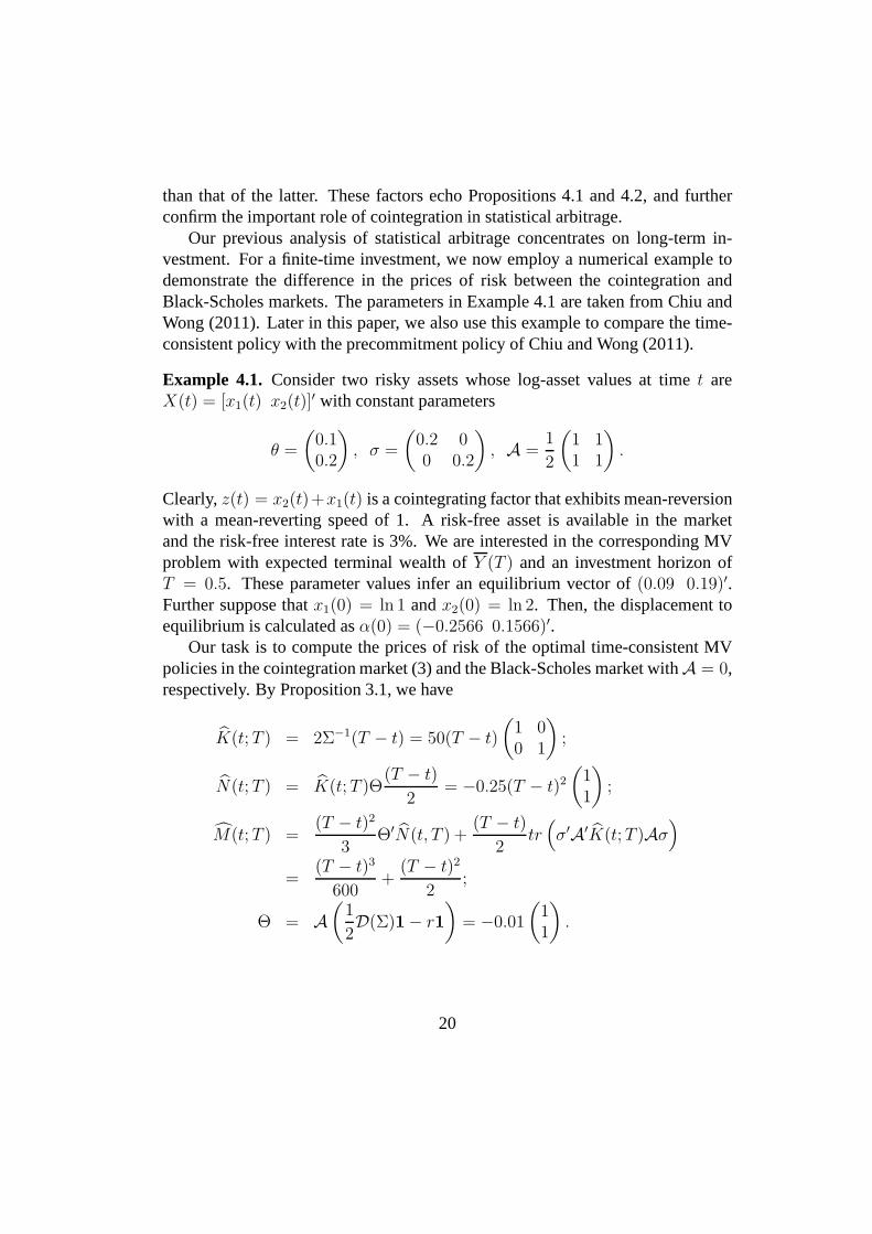
Our previous analysis of statistical arbitrage concentrates on long-term in-vestment. For a finite-time investment, we now employ a numerical example todemonstrate the difference in the prices of risk between thecointegration andBlack-Scholes markets. The parameters in Example 4.1 are taken from Chiu andWong (2011). Later in this paper, we also use this example to compare the time-consistent policy with the precommitment policy of Chiu andWong (2011).

Example 4.1. Consider two risky assets whose log-asset values at timet areX(t) = [x1(t) x2(t)]

′ with constant parameters

θ =

(0.10.2

), σ =

(0.2 00 0.2

), A =

1

2

(1 11 1

).

Clearly,z(t) = x2(t)+x1(t) is a cointegrating factor that exhibits mean-reversionwith a mean-reverting speed of 1. A risk-free asset is available in the marketand the risk-free interest rate is 3%. We are interested in the corresponding MVproblem with expected terminal wealth ofY (T ) and an investment horizon ofT = 0.5. These parameter values infer an equilibrium vector of(0.09 0.19)′.Further suppose thatx1(0) = ln 1 andx2(0) = ln 2. Then, the displacement toequilibrium is calculated asα(0) = (−0.2566 0.1566)′.

Our task is to compute the prices of risk of the optimal time-consistent MVpolicies in the cointegration market (3) and the Black-Scholes market withA = 0,respectively. By Proposition 3.1, we have

K(t; T ) = 2Σ−1(T − t) = 50(T − t)

(1 00 1

);

N(t; T ) = K(t; T )Θ(T − t)

2= −0.25(T − t)2

(11

);

M(t; T ) =(T − t)2

3Θ′N(t, T ) +

(T − t)

2tr(σ′A′K(t; T )Aσ

)

=(T − t)3

600+

(T − t)2

2;

Θ = A

(1

2D(Σ)1 − r1

)= −0.01

(11

).

20

By Proposition 3.3,

K(t, T ) = 2

∫ T

t

e1

2A′(t−s)Σ−1e−

1

2A(t−s)ds

= 25(1 − e−(T−t))

(1 11 1

)+ 25(T − t)

(1 −1−1 1

);

N(t, T ) =

∫ T

t

e−A′(t−s)K(s, T )Θds

=(1 + T − t)e−(T−t) − 1

2

(11

);

M(t, T ) =

∫ T

t

N(s, T )′Θ +1

2tr (σ′A′K(s, T )Aσ) ds

= 1.01(T − t) − 1.02 + (1.02 + 0.01(T − t))e−(T−t).

Substituting all of these into (48), we obtain a price of riskof 1.2634. The solidline in Figure 1 is the efficient frontier of trading for the cointegrated pair ofrisky assets in Example 4.1 and the risk-free bond, whereas the dashed line is thatfor the trading of similar risky assets in the Black-Scholesmarket, i.e.,A ≡ 0,and the risk-free bond. It can be seen that cointegration maygenerate a sizabledegree of statistical arbitrage profits. The expected terminal wealth of trading thecointegrated pair is significantly larger than that of trading the pair of stocks thatfollow geometric Brownian motions with the same volatilityand drifts equal tothe initial drifts of the cointegrated assets. In fact, the price of risk for the assetsfollowing the Black-Scholes dynamics is only 0.7621.

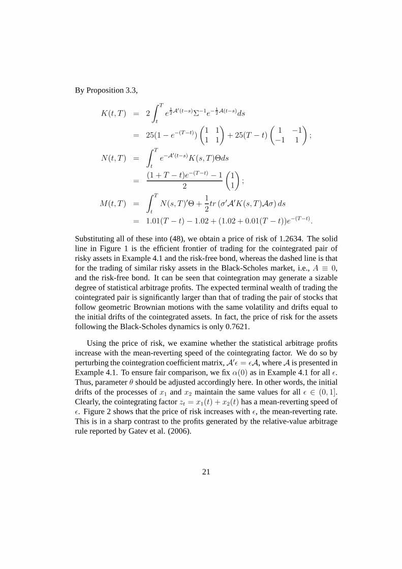
Using the price of risk, we examine whether the statistical arbitrage profitsincrease with the mean-reverting speed of the cointegrating factor. We do so byperturbing the cointegration coefficient matrix,A′ǫ = ǫA, whereA is presented inExample 4.1. To ensure fair comparison, we fixα(0) as in Example 4.1 for allǫ.Thus, parameterθ should be adjusted accordingly here. In other words, the initialdrifts of the processes ofx1 andx2 maintain the same values for allǫ ∈ (0, 1].Clearly, the cointegrating factorzt = x1(t) + x2(t) has a mean-reverting speed ofǫ. Figure 2 shows that the price of risk increases withǫ, the mean-reverting rate.This is in a sharp contrast to the profits generated by the relative-value arbitragerule reported by Gatev et al. (2006).

21

0 0.1 0.2 0.3 0.4 0.5 0.6 0.7 0.8 0.9 110

10.2

10.4

10.6

10.8

11

11.2

σY(T)

E[Y

(T)]

Cointegrating Factor = 1Cointegrating Factor = 0

Figure 1: Efficient frontiers of Example 4.1.

4.3 Comparison with the precommitment policy

As this paper considers the time-consistent MV optimal trading strategy, a naturalquestion is whether this strategy outperforms the precommitment policy obtainedin the literature. More precisely, how can we fairly comparethese two approachesfor dynamic MV portfolio selection problems? Wang and Forsyth (2011) havealready given a partial answer. Using a numerical scheme, they show numericallythat the price of risk from the precommitment policy is always higher than thatfrom the time-consistent policy in the Black-Scholes market. The fundamentalreason is that the time-consistent policy observes an additional constraint associ-ated with time-consistency (6). Wang and Forsyth (2011), however, argue that atime-consistent policy is still wealth considering as it makes economic sense.

The advantage of the time-consistent MV optimal policy can be articulated inthe cointegration financial market via a quantitative approach. We further confirmthat the price of risk from a precommitment policy is greaterin the cointegrationmarket. What makes the time-consistent policy appealing isits robustness andstability with respect to the estimated parameters. The precommitment policy inthe cointegration market involves solving a matrix Riccatidifferential equation(MRDE), which may cause a finite escape time at which the solution blows up toinfinity. This problem is hidden in the Black-Scholes market.

Consider the following initial optimal time-consistent and precommitment

22

0 0.1 0.2 0.3 0.4 0.5 0.6 0.7 0.8 0.9 11.48

1.5

1.52

1.54

1.56

1.58

1.6

1.62

1.64

1.66

ε

ρ

Figure 2: Statistical arbitrage profits and mean reverting rate.

policies.

u∗(0, X, T ) =Y T e−rT − Y0

H(0, α, T )

[(Σ−1 + A′K(0, T )

)α + A′N(0, T )

]and

u∗prec(0, X, T ) =

Y T e−rT − Y0

1 − G(0, α, T )

[(Σ−1 −A′KG(0, T )

)α −A′NG(0, T )

],

whereu∗prec(t, X, T ) denotes the precommitment policy derived by Chiu and Wong

(2011),

G(0, α, T ) = exp

−

1

2α′KG(0, T )α − N ′

G(0, T )α − MG(0, T )

,

with KG(t, T ) being solved by a MRDE,NG(t, T ) by a system of ODEs andMG(t, T ) by a linear ODE. To illustrate our ideas and get rid of the subtle calcu-lation associated with the MRDE, we employ Chiu and Wong’s (2011) exampleand the parameters in Example 4.1 directly:

KG(t, T ) =25 sin(T − t)

cos(T − t) − sin(T − t)

(1 11 1

)+ 25(T − t)

(1 −1−1 1

),

NG(t, T ) =1

2N(T − t)

(11

), N(τ) =

cos τ − 1

cos τ − sin τ,

MG(t, T ) =(T − t)

2+

ln | cos(T − t) − sin(T − t)|

2

23

+1

100

∫ T−t

0

(N(s)2 − N(s)

)ds.

It can be seen thatKG(0, T ), NG(0, T ) andMG(0, T ) diverge atT = π/4, makingu∗(0, X, π/4) diverge as well.

0 50 100 1504

6

8

10

12

14

16T= 1 month

σY(T)2

E[Y

(T)]

PrecommitmentTime−consistent

0 20 40 604

6

8

10

12

14

16T= 2 months

σY(T)2

E[Y

(T)]

PrecommitmentTime−consistent

0 20 404

6

8

10

12

14

16T=3 months

σY(T)2

E[Y

(T)]

PrecommitmentTime−consistent

0 10 20 304

6

8

10

12

14

16T=4 months

σY(T)2

E[Y

(T)]

PrecommitmentTime−consistent

0 10 204

6

8

10

12

14

16T=5 months

σY(T)2

E[Y

(T)]

PrecommitmentTime−consistent

0 10 204

6

8

10

12

14

16T= 6 months

σY(T)2

E[Y

(T)]

PrecommitmentTime−consistent

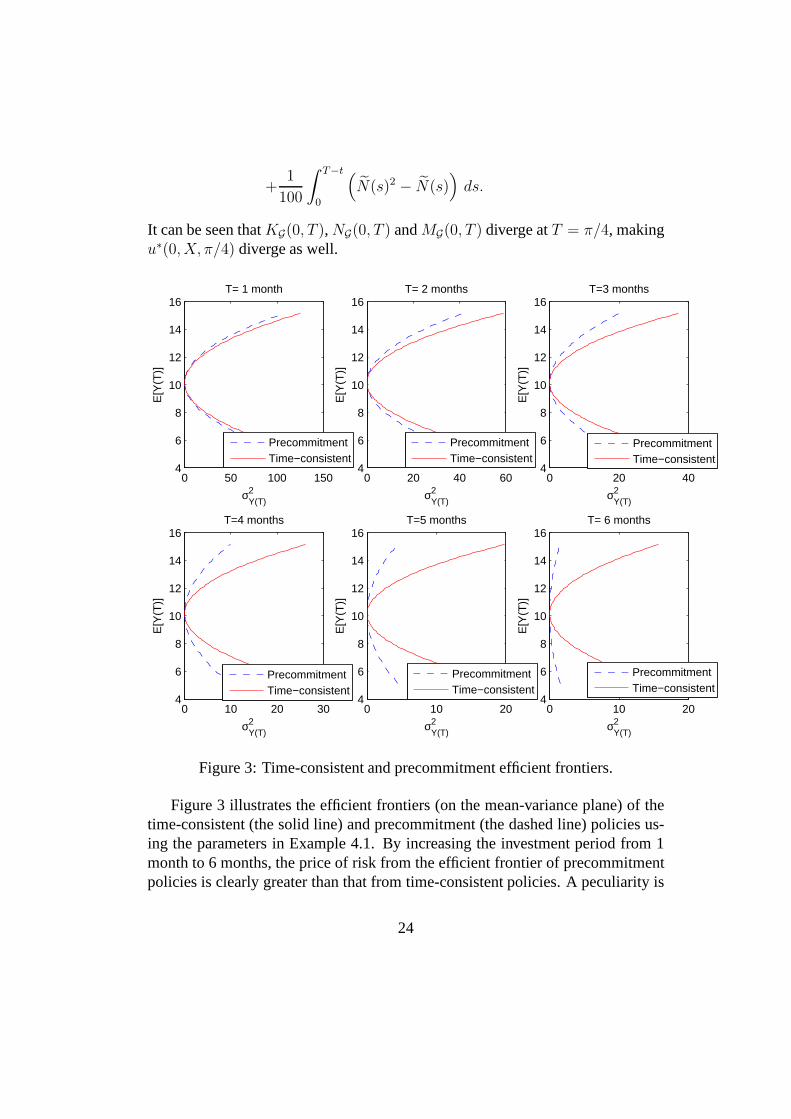
Figure 3: Time-consistent and precommitment efficient frontiers.

Figure 3 illustrates the efficient frontiers (on the mean-variance plane) of thetime-consistent (the solid line) and precommitment (the dashed line) policies us-ing the parameters in Example 4.1. By increasing the investment period from 1month to 6 months, the price of risk from the efficient frontier of precommitmentpolicies is clearly greater than that from time-consistentpolicies. A peculiarity is

24

that the efficient frontier of precommitment policies is an almost vertical line for6-month investments, indicating almost perfect arbitrage. This is too good to betrue. The time-consistent efficient frontier also has an increasing price of risk, butis much more persistent.

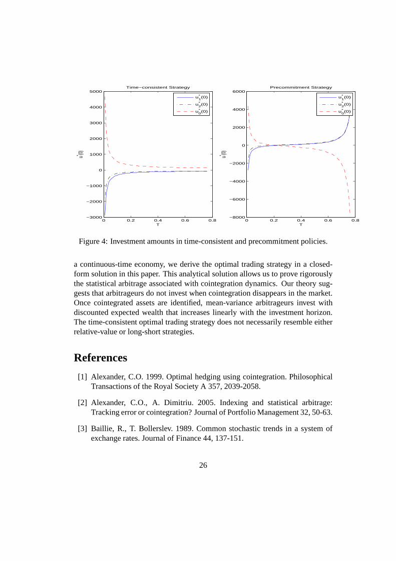
Important insights can be drawn by examining the optimal policies directly.Figure 4 shows the initial investment amounts in the risk-free asset (u∗

0), asset1 (u∗

1) and asset 2 (u∗2) under the assumption in Example 4.1 and the conditions

thatY T e−∫ T

0r(s)ds = $20 andY0 = $10. The investment period, however, varies

from 0.001 to 0.76 years. For a short-term investment, the two policies are sim-ilar but the precommitment policy diverges when the investment period close to0.76 ≃ π/4. It can be shown by Lemma 4.2 in Chiu and Wong (2011) that thehigher the mean reversion speed, the shorter the escape time. As the mean rever-sion speed in practice is usually of an order of10−3 or even less, it is difficult todetect the problem. The implication of this example is essentially concerned withthe sensitivity and robustness of the portfolio policy to the estimated parameters.In practice, the cointegration matrixA and the other parameters are always esti-mated with errors. When the parameters are combined to estimate the mean rever-sion rate, the aggregate error has a greater impact on the optimal precommitmentpolicy than the time-consistent policy. The aggregate estimation error is, how-ever, difficult to control (Tang and Chen, 2009). The time-consistent MV policy ispreferred for its robustness to the estimated parameters. Whereas the optimal pre-commitment policy can aggressively take full advantage of the assumed model,because it considers a generic set of trading policies, the optimal time-consistentpolicy is primarily concerned with rational decisions. Theimprecise estimation ofthe assumed model thus becomes an additional factor to be considered in practice.

The policies shown in Figure 4 also demonstrate that the dynamic MV trad-ing of cointegrated assets may resemble neither relative-value nor long-short ar-bitrage. Both precommitment and time-consistent policiestypically leverage byshorting all risky assets for the risk-free bond for investment horizons less than0.1 years. The precommitment policy alone becomes a long-short strategy for aninvestment horizon longer than 0.3 years.

5 Conclusion

Although the trading of cointegrated assets is believed to be able to generate sta-tistical arbitrage profits, this belief has lacked rigoroustheoretical support. Byinvestigating time-consistent MV portfolio strategies for cointegrated assets in

25

0 0.2 0.4 0.6 0.8−3000

−2000

−1000

0

1000

2000

3000

4000

5000Time−consistent Strategy

T

u* (0)

u1* (0)

u2* (0)

u0* (0)

0 0.2 0.4 0.6 0.8−8000

−6000

−4000

−2000

0

2000

4000

6000Precommitment Strategy

Tu* (0)

u1* (0)

u2* (0)

u0* (0)

Figure 4: Investment amounts in time-consistent and precommitment policies.

a continuous-time economy, we derive the optimal trading strategy in a closed-form solution in this paper. This analytical solution allows us to prove rigorouslythe statistical arbitrage associated with cointegration dynamics. Our theory sug-gests that arbitrageurs do not invest when cointegration disappears in the market.Once cointegrated assets are identified, mean-variance arbitrageurs invest withdiscounted expected wealth that increases linearly with the investment horizon.The time-consistent optimal trading strategy does not necessarily resemble eitherrelative-value or long-short strategies.

References

[1] Alexander, C.O. 1999. Optimal hedging using cointegration. PhilosophicalTransactions of the Royal Society A 357, 2039-2058.

[2] Alexander, C.O., A. Dimitriu. 2005. Indexing and statistical arbitrage:Tracking error or cointegration? Journal of Portfolio Management 32, 50-63.

[3] Baillie, R., T. Bollerslev. 1989. Common stochastic trends in a system ofexchange rates. Journal of Finance 44, 137-151.

26

[4] Basak, S., G. Chabakauri. 2010. Dynamic mean-variance asset allocation.Review of Financial Studies 23, 2970-3016.

[5] Bielecki, T., H. Jin, S. R. Pliska, X.Y. Zhou. 2005. Continuous-time mean-variance portfolio selection with bankruptcy prohibition. Mathematical Fi-nance 15, 213-44.

[6] Bjork, T., A. Murgoci, X.Y. Zhou. 2011. Mean-variance portfolio optimiza-tion with state dependent risk aversion. Working paper, Oxford University,Nomura Centre for Mathematical Finance.

[7] Cerchi, M., A. Havenner. 1988. Cointegration and stock prices: The randomwalk on Wall Street revisited. Journal of Economic Dynamics& Control 12,333-346.

[8] Chiu, M.C., H.Y. Wong. 2011. Mean-variance portfolio selection of cointe-grated assets. Journal of Economic Dynamics & Control 35, 1369-1385.

[9] Cui, X.Y., D. Li, S.Y. Wang, S.S. Zhu. 2010. Better than dynamic mean-variance: Time inconsistency and free cash flow stream, Mathematical Fi-nance, forthcoming.

[10] Duan, J.C., S.R. Pliska. 2004. Option valuation with co-integrated assetprices. Journal of Economic Dynamics & Control 28, 727-754.

[11] Engle, R., C. Granger. 1987. Co-integration and error correction: Represen-tation, estimation and testing. Econometrica 55, 251-276.

[12] Gatev, E., W.N. Goetzmann, K.G. Rouwenhorst. 2006. Pairs trading: Per-formance of a relative-value arbitrage rule. Review of Financial Studies 19,797-827.

[13] Granger, C. 1981. Some properties of time series data and their use in econo-metric model specification. Journal of Econometrics 23, 121-130.

[14] Hogan, S., R. Jarrow, M. Teo, M. Warachkac. 2004. Testing market effi-ciency using statistical arbitrage with applications to momentum and valuestrategies. Journal of Financial Economics 73, 525-565.

[15] Jurek, J.W., H. Yang. 2007. Dynamic portfolio selection in arbitrage. Work-ing paper, Harvard Business School.

27

[16] Li, D., W.L. Ng. 2000. Optimal dynamic portfolio selection: Multiperiodmean-variance formulation. Mathematical Finance 10, 387-406.

[17] Liu, J., F.A. Longstaff. 2003. Losing money on arbitrage: Optimal dynamicportfolio choice in markets with arbitrage opportunities.Review of FinancialStudies 17, 611-641.

[18] Markowitz, H. 1952. Portfolio selection. Journal of Finance 7, 77-91.

[19] Strotz, R. H. 1956. Myopia and inconsistency in dynamicutility maximiza-tion. Review of Economic Studies 23, 165-80.

[20] Tang, C.Y., S.X. Chen. 2009. Parameter estimation and bias correction fordiffusion processes. Journal of Econometrics 149, 65-81.

[21] Taylor, M., I. Tonks. 1989. The internationalisation of stock markets and theabolition of U.K. exchange control. Review of Economics andStatistics 71,332-336.

[22] Vidyamurthy, G. 2004. Pairs Trading – Quantitative Methods and Analysis,Wiley: New York.

[23] Wachter, J.A. 2002. Portfolio and consumption decisions under mean-reverting returns: An explicit solution for complete market. Journal of Fi-nancial and Quantitative Analysis 37, 63-91.

[24] Wang, J., P.A. Forsyth. 2011. Continuous time mean variance asset alloca-tion: A time consistent strategy. European Journal of Operational Research209, 184-201.

[25] Zhou X.Y., D. Li. 2000. Continuous-time mean-varianceportfolio selection:A stochastic LQ framework. Applied Mathematics & Optimization 42, 19-33.

A Proof of Lemma 3.1

To simplify matters, we writeJ(t) = J(t, Y (t), X(t)). By the time-consistentproperty (6), for any0 < τ < T − t,

J(t) = minu∈U(t,T )

Var(Y (T )|Ft) − 2λE[Y (T )|Ft]

28

= minu∈U(t,t+τ)

E[J(t + τ)|Ft] + Var(E[Y ∗(T )|Ft+τ ]|Ft),

whereY ∗(T ) is the terminal wealth with the optimal control adopted. Letu∗

denote the optimal policy. By (10) and the definition ofΓ in (15), we obtain anexpression of E[Y ∗(T )|Ft+τ ] which brings us the following.

0 = minu∈U(t,t+τ)

E[J(t + τ) − J(t)|Ft] + Var(e∫ T

t+τr(s)dsY (t + τ) + Γ(t + τ)|Ft

)

= minu∈U(t,t+τ)

Var(

e∫ T

t+τr(s)dsY (t + τ) − e

∫ T

tr(s)dsY (t) + Γ(t + τ) − Γ(t)

∣∣∣Ft

)

+E[J(t + τ) − J(t)|Ft]

. (55)

Thus, (14) follows by lettingτ → 0 in equation (55).To derive an expression for the optimal time-consistent trading strategyu∗(t),

we solve equation (14). By (12), we have

E[dJ |Ft] = E[−2λe

∫ T

tr(s)dsα(t)′u(t)dt + dJ1

∣∣∣Ft

]. (56)

Applying Ito’s lemma toΓ yields

dΓ =

[∂Γ

∂t+

(∂Γ

∂X

)′

(θ −AX) +1

2tr

(σ′ ∂

2Γ

∂X2σ

)]dt +

(∂Γ

∂X

)′

σdWt, (57)

which impliesbthat

Var(

d(e∫ T

tr(s)dsY (t)

)+ dΓ

∣∣∣Ft

)

= E

[e2∫ T

tr(s)dsu′Σu + 2e

∫ T

tr(s)dsu′Σ

∂Γ

∂X+

∂Γ

∂X

′

Σ∂Γ

∂X

∣∣∣∣Ft

]dt. (58)

Substituting (13), (56) and (58) into (14) produces a straightforward quadraticminimization problem with respect tou. A simple completing square methodgives the optimal policy in (16).

B Proof of Proposition 4.1

Substituting conditionsY0 = 0 and E[YT ] = η(T ) exp(∫ T

0r(s)ds) into (32) allows

to solve forλ such that

λ =η(T )e

∫ T

0r(s)ds

H(0, α(0), T )> 0.

29

To prove (51), consider the dynamics of the optimal wealth level in (35):

Y ∗T = Γ(0, X(0), T ) + λ

∫ T

0

α′(s)Σ−1σdWs

= λH(0, α(0), T ) + λ

∫ T

0

α′(s)Σ−1σdWs,

whereλ andH are positive. AsPY ∗T < 0 = Pe

∫ T

0r(s)dsY ∗

T < 0, we concen-trate on the former probability.

PY ∗T < 0 = P

λH(0, α(0)) + λ

∫ T

0

α′(s)Σ−1σdWs < 0

= P

−

∫ T

0

α′(s)Σ−1σdWs > H(0, α(0))

≤ P

∣∣∣∣−∫ T

0

α′(s)Σ−1σdWs

∣∣∣∣ > H(0, α, T )

≤Var(∫ T

0α′(s)Σ−1σdWs

)

H(0, α, T )2(59)

=E[∫ T

0α′(s)Σ−1α(s)ds

]

H(0, α, T )2=

H(0, α, T )

H(0, α, T )2. (60)

The Chebyshev inequality is applied in (59). It suffices for us to prove that theupper bound of the probability in (60) goes to zero whenT tends to infinity. Todo so, we investigate the asymptotic properties ofH(0, α, T ) andH(0, α, T ) fora largeT .

Let Pm(T ) be the set of polynomials inT of an order no greater thanm forsome integerm. By Proposition 3.1, we have

H(0, α, T ) =1

2α′K(0, T )α + N(0, T )′α + M(0, T ),

where, under the assumption of constant parameters,

K(0, T ) = 2Σ−1T, N(0, T )′ = Θ′Σ−1T 2 (61)

M(0, T ) = Θ′Σ−1ΘT 3

3+ tr

(σ′A′Σ−1Aσ

) T 2

2.

Therefore,H(0, α, T ) ∈ P3(T ). If A 6= 0, thenΘ′Σ−1Θ > 0 andH(0, α, T )

diverges to infinity with the same order asT 3. Hence, we writeH(0, α, T ) ∼

30

O(T 3) in this case. Alternatively, ifA = 0, thenΘ = 0 andH(0, α, T ) ∈ P1(T ).We denoteH(0, α, T ) ∼ O(T ) in this latter case.

By Proposition 3.2, we have

H(0, α, T ) =1

2α′K(0, T )α + N(0, T )′α + M(0, T ),

where

K(t, T ) = 2

∫ T

t

e1

2A′(t−s)Σ−1e

1

2A(t−s)ds,

N(t, T )′ =

∫ T

t

Θ′K(s, T )eA(t−s)ds,

M(t, T ) =

∫ T

t

N(s, T )′Θ +1

2tr (σ′A′K(s, T )Aσ)ds.

The limiting property ofH(0, α, T ) can then be assessed by investigating the lim-iting properties ofK, M andN . It is obvious thatH(0, α, T ) = 2α′Σ−1αT andH ∼ O(T ) onceA = 0.

We focus on the case in whichA 6= 0 and the eigenvalues are nonnegative.By the Cayley-Hamilton theorem on matrix exponential functions, for anyn × nconstant matrixA,

e−At = B +

n−1∑

i=0

ci(t)Ai, (62)

where

ci(t) =k∑

m=1

fim(t)e−γmt, (63)

k ≤ n is the number of non-zero eigenvalues ofA (or rank(A)); γm are the non-zero eigenvalues ofA for m = 1, 2, . . . , k; fim(t) ∈ Pk(t) for all i = 0, . . . , n− 1andm = 1, · · · , k; andB is ann × n constant matrix. The assumption on matrixA implies thatγm are positive for allm = 1, 2, . . . , k. For such a matrixA, asci(t) decays to zero in an exponential order oft for all i = 0, . . . , n− 1, it is clearthat, for any finite integersn0, . . . , nm′ andm′,

limt→∞

m′∏

j=0

n−1∏

i=0

ci(t)nj = 0,

31

limT→∞

1

T

∫ T

0

m′∏

j=0

n−1∏

i=0

ci(t)njdt = 0. (64)

Consider the matrix-valued functionK(0, T ) in (38), which diverges whenTgoes to infinity. By L’Hopital’s rule, we have

limT→∞

K(0, T )

T= lim

T→∞

∂

∂TK(0, T )

= limT→∞

2e−A′T/2Σ−1e−AT/2 = 2B′Σ−1B, (65)

where the last equality holds by (62). Hence, we writeK(0, T ) ∼ O(T ).The vector-valued functionN(0, T ) in (39) also diverges withT as it is an

integration ofK(t, T ). Thus, we apply L’Hopital’s rule to the following limit.

limT→∞

N(0, T )′

T 2= lim

T→∞

Θ′

T 2

∫ T

0

K(s, T )e−Asds

= limT→∞

Θ′

2T

∫ T

0

∂

∂TK(s, T )e−Asds

= limT→∞

Θ′

T

∫ T

0

e1

2A′(s−T )Σ−1e

1

2A(s−T )e−Asds.

By (62) and (64), we have

limT→∞

N(0, T )′

T 2= Θ′B′Σ−1B2. (66)

Hence,N(0, T ) ∼ O(T 2).Applying similar tricks toM(0, T ) with some simple but tedious calculations

shows thatM(0, T ) ∼ O(T 3). Hence,H(0, α, T ) ∼ O(T 3).Substituting all of these into (60), we conclude that

PY ∗T < 0 ≤

H(0, α, T )

H(0, α, T )2∼

O(T )O(T 2)

, if A = 0O(T 3)O(T 6)

, if A 6= 0→ 0. (67)

This completes the proof for (51).We now prove (52). By Proposition 3.3 and (67), we have

Var(e−∫ T

0r(s)dsY ∗

T ) = η(T )2 H(0, α, T )

H(0, α, T )2∼

η(T )2

O(T ), if A = 0

η(T )2

O(T 3), if A 6= 0

.

32

The condition (50) is sufficient to ensure that

limT→∞

Var(e−∫ T

0r(s)dsY ∗

T )

T= 0

for A 6= 0. Alternatively, we additionally require thatC = 0 in (50) to have thelimit approaching zero forA = 0.

Finally, consider the case in whichA has a negative eigenvalue. In (63),ci(t)diverges to infinity with an exponential order oft. It turns out thatH(0, α, T )

tends to infinity with an exponential order ofT andH(0, α, T ) tends to infinitywith the degree 3 polynomial order ofT . By Proposition 3.3, the variance in (52)diverges.

33