


Languages
Pages
Legal

Computer Science and Information Systems 18(3):687–702 https://doi.org/10.2298/CSIS200130048G
DrCaptcha: An Interactive Machine Learning
Application
Rafael Glikis, Christos Makris, and Nikos Tsirakis
Computer Engineering and Informatics Department,
University of Patras,
26500 Patras, Greece
{rglykys, makri, tsirakis}@ceid.upatras.gr
Abstract. The creation of a Machine Learning system is a typical process that is
mostly automated. However, we may address some problems in the during
development, such as the over-training on the training set. A technique for
eliminating this phenomenon is the assembling of ensembles of models that
cooperate to make predictions. Another problem that almost always occurs is the
necessity of the human factor in the data preparation process. In this paper, we
present DrCaptcha [15], an interactive machine learning system that provides
third-party applications with a CAPTCHA service and, at the same time, uses the
user's input to train artificial neural networks that can be combined to create a
powerful OCR system. A different way to tackle this problem is to use transfer
learning, as we did in one of our experiments [33], to retrain models trained on
massive datasets and retrain them in a smaller dataset.
Keywords: machine learning, neural networks, transfer learning, interactive
machine learning, ensemble techniques.
1. Introduction
A typical process for building a machine learning system starts with the preparation of
the data by an expert. This process could be very long and expensive since it must be
done manually. Then follows the construction of a model using a learning algorithm on
these data. After training, the model is evaluated and if its performance is satisfiable it
can be used for predictions in unseen data? But if not this long training process starts
again after tweaking the parameters of the learning algorithm. This procedure, many
times involves a little trial and error and is repeated until the model performance is
sufficient. Depending on the learning algorithm, the size of the training set and the
hardware used this process could take from some hours to months! Another problem that
occurs very often during the training phase is the over-fitting of the trained model to the
training data. That makes the model lose its ability to generalize on unseen data. In this
paper, we will try to tackle those problems by using transfer learning [20], ensemble
[11] and interactive machine learning [18] techniques as proof of concept.
First, let's take the problems one by one. In order to start training a model, we need to
have a sufficient amount of labeled data, and very often the labeling of this dataset must
be done by a human. Our approach to this issue is to outsource the labeling to a service

688 Rafael Glikis, Christos Makris, and Nikos Tsirakis
we created, that will be used by third-party applications, and use the user's data to
prepare our dataset. The next problem we face is the long training time that does not
allow the fast formation of a model along with the overtraining of the model in the
training set. Our approach to this problem is not overcomplicating things and create
simple and neat machine learning models that can be trained in a very short time and
give us feedback very fast. But this comes with a price, since the simple models may not
be as accurate as the complex models. To overcome this issue we can construct
ensembles of models and use those instead. Most of the time we will find out that the
ensemble generalizes better than any of the models that make it up. This technique is
also useful when the training set is very small and/or the learning algorithm becomes
prone to over-fitting.
Having that in mind, we developed “DrCaptcha” a machine learning application that
will serve as a Proof of Concept for the solutions we are proposing. “DrCaptcha” is an
interactive machine learning (iML) application. The purpose of this application is to
take advantage of the feedback provided by users and use it to optimize a machine
learning model. The purpose of this model is to perform Optical Character Recognition
(OCR) on handwritten characters. The latter has attracted the interest of many
researchers [5, 6, 7, 8, 9, 13] with very good results. Our solution to the problem focuses
primarily on the minimization of the data preparation phase. We then focus on the speed
of the training phase along with the avoidance of overfitting. Our goal was to achieve
state-of-the-art results with the above limitations.
“DrCaptcha“ initially provides users with an automated CAPTCHA system with the
ability to distinguish whether the user is a human or a machine. The system then
compares the values given by the user with the values stored in the database for the
CAPTCHA, and if these values match then the system recognizes that the user is human
and otherwise not.
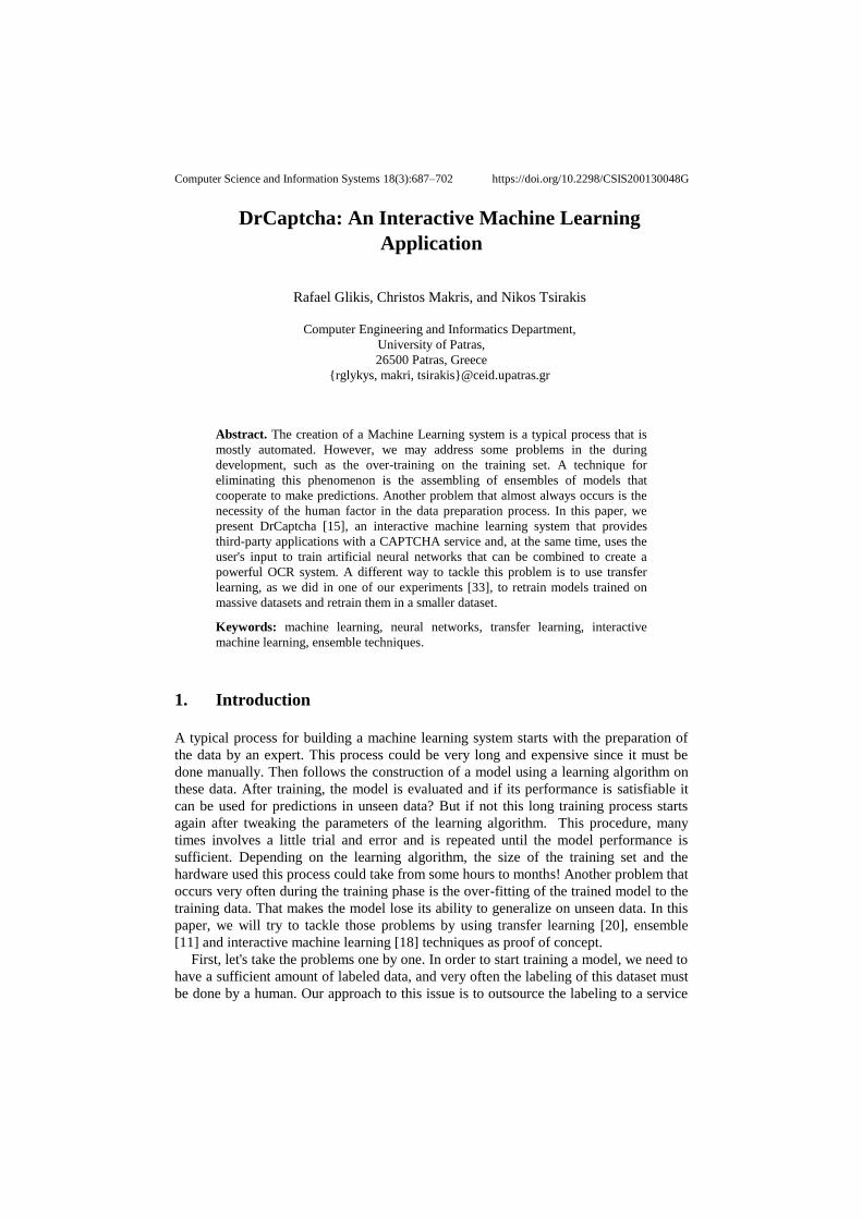
The difference of this system from the classic CAPTCHA systems is that the system
itself, for some of the images, does not know all the characters. If the system verifies
that the user input matches the data in the database, it will take the user values for the
non-classified digits, and classify them according to the values given by the user (see
Fig. 1.). In case the user login is incorrect, the system will not classify the characters. In
this way, the user provides implicit feedback to the system by classifying characters,
which will be used later to train machine learning models. This functionality is available
through a GUI and an API.
Based on the classified characters the application trains some artificial neural
networks. After training and evaluating them, stores their training parameters, structure,
and the confusion matrix. The latter will be used to synthesize ensembles of models that
operate in the manner described later in this paper.
After the training of the neural networks, an administrator can create an ensemble of
neural networks and assign weights to each of them. This ensemble acts as a meta-model
that takes the prediction from the base classifiers and then decides which prediction to
output. When a user creates or makes a change to this ensemble, the application
evaluates it using a test set and saves its parameters again.
DrCaptcha: An Interactive Machine Learning Application 689
Fig. 1. How our CAPTCHA service works
Finally, the application provides a more interactive evaluation method where the user
can "paint" a character and ask the system which character it is. The system will then
retrieve the ensemble with the highest accuracy from the database, and give the user its
prediction.
Also, if the base classifiers disagree and there are more than one dominant
predictions, the system may come up with alternative results for an input. This can be
extremely useful for an optical character recognition system. For example with the
addition of some extra rules, even word corrections can be made. One possible solution
that takes advantage of this feature is, for the system to be expanded to use a dictionary,
and look at the different predictions given by the neural network ensemble, and
comparing them with the dictionary, making the necessary corrections until the word
matches with a word in the dictionary.
2. Related Work
2.1. Interactive Machine Learning
Interactive Machine Learning (iML) is a very promising tool for enhancing both human
and computer capabilities. In the past, attempts have been made to create classifiers
from humans manually using interactive machine learning systems. Those systems
usually follow the same pattern - the training of a machine learning model using training
data, and the evaluation of this model by a human. The feedback from this evaluation is
considered for the creation of another model. This process repeats until the model
performance is sufficient.
One interesting iML application is CueFlik [1]. CueFlik is an image web search
application that allows users to quickly create their own rules for re-ranking images
based on their visual characteristics. Users can then re-rank any future Web image
search results according to their rule. This approach can extend the capabilities of
existing computer vision methods to make a web search application more efficient.

690 Rafael Glikis, Christos Makris, and Nikos Tsirakis
ReGroup [2] (Rapid and Explicit Grouping) is a system that applies end-user
interactive machine learning to help people create custom, on-demand groups in online
social networks. It works by observing a person’s normal interaction of adding members
to a group while learning a probabilistic model of group membership which it uses to
suggest both additional members and group characteristics for filtering a friend list.
Also, some attempts have been made to enable users to explicitly create classifiers.
These methods are particularly helpful because an expert should not expect the
automatic algorithm to discover something obvious. When such systems used by a
domain expert, background knowledge is automatically exploited because the user is
involved in almost every decision that leads to the induced models.
In [3], an interactive machine learning system was put in place which enabled its
users to create a decision tree with a graphical environment by drawing a line between
the points (corresponding to samples) that were graphically represented for a feature
using in a two-dimensional visual interface. In [4] transparent boosting tree was
proposed which visualizes both the model structure and prediction statistics of each step
in the learning process of gradient boosting tree to user, and involves user’s feedback
operations to trees into the learning process such as add/remove a tree, select feature
group for building a new tree, remove a node on the current tree and expand a leaf node.
The system also allows the users to go back to any previous model in the learning loop.
2.2. Optical Character Recognition with Neural Networks
One of the most prevalent methods of machine learning is artificial neural networks.
EMNIST [8] is the widely used benchmark for the hand-written recognition task.
Multiple works [5, 6, 7, 8, 9, 13] have used machine learning models on the EMNIST
dataset and have achieved very good results.
In [8], EMNIST’s balanced dataset used as input for both a linear classifier and
OPIUM-Based classifiers [10] with a different number of hidden neurons each. [6]
proposed a deep neural network that is composed of two auto-encoder layers, with 300
and 50 neurons respectively and one softmax layer. [7] proposed a neuro-evolutionary
algorithm that evolves simple and successful architectures built from embedding, 1D
and 2D convolutional, max pooling and fully connected layers along with their hyper-
parameters.
2.3. Ensemble Techniques
Such methods improve the predictive performance of a single model by training multiple
models and combining their predictions. In the past, several attempts have been made in
creating ensembles, with impressive results [11].
One way to increase the performance of a machine learning model is to learn multiple
weak classifiers and boost their performance using a boosting algorithm. One
disadvantage of those is that they require re-training based on the misclassified samples,
and this may slow down the learning process. [12] proposed an aggregation technique
that combines the output of multiple weak classifiers that do not require any re-training.

DrCaptcha: An Interactive Machine Learning Application 691
As a result, the training process is very fast while the model achieves state-of-the-art
results. Another advantage of this framework is that it can combine classifiers that were
created using different algorithms.
In recent years there have been a few attempts to combine the ensemble techniques
and deep neural networks approaches [11]. While most of them center around
developing an ensemble of deep individual neural networks, techniques like dropout
split the initial neural network into several pieces at training time, to avoid over-fitting.
Such techniques aim to reduce complex co-adaptations of neurons since a neuron cannot
rely on the presence of particular other neurons in an individual neural network. Thus
the neural network is forced to learn more robust features [16].
2.4. Transfer Learning
As stated earlier in this paper, the collection of data is complicated and expensive,
making it extremely difficult to build a large-scale, high-quality annotated dataset due to
the expense of data acquisition and labeling. Transfer learning [20] is the methodology
of transferring knowledge from a source domain to a target domain. Usually, the size of
the source domain is much larger. This process enables us to tackle problems with
insufficient training data, which has a tremendously positive effect on many areas that
are difficult to improve because of inadequate training data [21]. The main idea is that a
deep neural network learning process is similar to the processing mechanism of the
human brain, and it is an iterative and continuous abstraction process. The network's
front-layers can be treated as a feature extractor and identify low-level features of
training data. At the same time, subsequent layers can extract more high-level features
that provide the network with the information needed to make the final decision.
By assuming that the neural network can learn low-level features from another
dataset, we can take a neural network train it on a huge dataset, acquire a lot of low-level
features, and retrain a part or all of it with a smaller dataset. This process will enable our
model to take advantage of the low-level features learned from the first dataset and
combine them with the high-level features learned from the second smaller one to make
better predictions. For example in [22] the Inception-v3 [28] was used with weights
trained on ImageNet [26] dataset and achieved 70.1% accuracy on CIFAR-10 dataset
[23] and 96.5% on Caltech Faces dataset [24]. While transferring knowledge from a
model trained on a labeled dataset is ideal, we can also transfer knowledge from models
trained on unlabeled datasets. In [25], a new machine learning framework was develop
called “self-taught learning” that uses models trained using unlabeled data for
classification tasks. Another benefit that emerges is that the first half of the process - the
training on the huge dataset - can be done once and use the low-level features learned on
various more specialized datasets making the training cycle for these much smaller.
3. Ensemble Methodology
The method described in this section is an ensemble technique that uses artificial neural
networks as base classifiers. Any type of neural network could be used. The only

692 Rafael Glikis, Christos Makris, and Nikos Tsirakis
limitation is for the classifier to give the normalized probabilities for each category as a
result. Although we are using neural networks, any type of classifier could be used as
long as the above limitation applies.
This method combines a series of models of artificial neural networks (base
classifiers), M1, M2, . . . , Mk, aiming at creating an improved model, M*. To understand
this concept, let's say we have a patient and we want to make a diagnosis based on his
symptoms. Rather than asking for a doctor's opinion, we can ask for an opinion from
many. So if we see that the majority of doctors agree on a diagnosis, then we can choose
it as the final diagnosis. The final diagnosis can be made by a majority, where the vote
of each doctor has the same weight. The majority of voters of a large group of doctors
may be more reliable than majority voting by a small group or only one. This is the case
in most cases for an ensemble of classifiers.
The structure of artificial neural networks is not particularly relevant, as long as the
last layer has a softmax activation so that the output layer gives us what normalized
probability that the input sample can belong to. Let us call this probability pi,j where i
denote the class, and with j the model from which it emerged. That is, the probability pi,j
is the probability for class i by the artificial neural network j. We also can have k
training sets, D1, D2,. . . , Dk, where Di (1 ≤ i ≤ k) is used to create the Mi classifier.
Each of the models of artificial neural networks M1, M2,. . . , Mk has a weight
w1, w2,. . . , wk which is normalized so that the total weights for all artificial neural
networks are 1. Continuing with the previous example, we assume that we place weights
on the value of diagnosis for each doctor, based on the accuracy of previous diagnoses
they have made or based on their specialty. The final diagnosis is then a combination of
weighted diagnoses. In the case of artificial neural networks, we can compare education
with the training parameters and the structure of the neural network. An examination of
previous diagnoses can be likened to the examination of the confusion matrix.
Let us now pass a sample X as an input to all artificial neural networks. At the final
layer of each model Mi, we will have the probability of each class for the input. Then we
multiply all outputs of the artificial neural network Mi with the weight of the artificial
neural network. The same action will be done for all neural networks of the ensemble,
and at the end of the process, the probabilities of each model will be added by category,
with the corresponding categories of all the models of the ensemble. The category with
the largest sum of probabilities will be the output class.
Fig. 2. shows schematically how this method works. On the left side are the base
classifiers. On each base classifier, each output neuron is associated with the
corresponding neuron that handles the class. The above structure looks intuitive to an
artificial neural network in which the output layer is not connected with all the neurons
of the previous layer.
This process is mathematically described by Eq. 1. and Eq. 2. In those, with P i we
denote the sum of the probabilities for class i by all neural networks. With pi,j we denote
the probability given by the network j the class, for the class i. With wj we denote the
weight of the neural network j, while the number of classes is c.
Pi= ∑j= 1
k
pi , j w j
(1)

DrCaptcha: An Interactive Machine Learning Application 693
class= argmax(P1, P2,...,Pc) (2)
The advantage of this method is that it does not only take into account the only
prediction made by neural networks. The result is deduced from the probabilities given
by artificial neural networks for each class as output. Thus, the result is not only
deducted as a weighted vote but also the confidence of the base classifiers in their
prediction. Continuing our diagnosis example, now we take into account the confidence
of each doctor along with the previous ones.
As for the choice of weights for each artificial neural network, this can be done
automatically by considering the accuracy of the model in a validation set with Eq. 3
where wi is the weight for neural network i, ai is the accuracy of the neural network i,
and k is the total number of neural networks in the ensemble.
wi=a
i
∑j= 1
k
aj
(3)
This setting can also be done manually by an administrator who can adjust weights by
looking at the accuracy of each neural network and other statistics. Those statistics could
be different metrics such as precision, sensitivity, specificity, and f-mesure or additional
insights we can extract from the confusion matrix of the ensemble and each base
classifier. The administrator could also consider the data gathered during each base
classifier's training phase, such as the number of epochs, batch size, the increase or
decrease of loss, and accuracy on each epoch indicating the level of over-training of
each classifier.
Last but not least, the administrator should manually test the ensemble with their data
(excluding train and test set), see how the ensemble and each base classifier behave and
adjust the weights accordingly. Repeating this process multiple times ensures the
classifier's quality and, with each iteration, enhances the ensemble more and more with
human expertise.
The whole process can be summarized by the following Аlgorithm 1.
Algorithm 1. The proposed algorithm
1. Training:
1. Train all base classifiers (neural networks) with the training
set(s).
2. Test all base classifiers with a test set.
3. Manually add weights to the base classifiers. (Add more base
classifiers to the ensemble and adjust weights)
2. Prediction:
1. Make predictions with all the base classifiers and extract the
probabilities for each one.
2. Compute the overall probability for each class.
3. The ensemble prediction is the class with the highest
probability.

694 Rafael Glikis, Christos Makris, and Nikos Tsirakis
Fig. 2. Schematic representation for the proposed model

DrCaptcha: An Interactive Machine Learning Application 695
4. Context of Experimental Study
To test this methodology, we created two ensembles on two different datasets. The first
one was capable of performing optical character recognition tasks, while the second one
was a system that can detect pneumonia from chest x-rays. The base classifiers used in
the first set of experiments were custom made neural networks (shallow, deep, and
convolutional). However, on the second set of our experiments, we used existing state-
of-the-art neural network architectures with some modifications to prepare them for the
task. This way, we can confirm that our methodology works regardless of the
architecture used.
4.1. Optical Character Recognition System
The OCR system predicts handwritten digits, uppercase, and lowercase characters. The
dataset used for training was the EMNIST’s balanced dataset which consists of 47
classes. For the creation of this system, we designed four neural networks which are
described later in this section. Then we used these networks to assemble an ensemble.
The first artificial neural network to be implemented is a simple neural network with
10000 hidden neurons. The network takes an image (matrix) of 28x28 as input and
converts it to a vector of size 784. Then it passes this image from a dense layer with
10000 neurons using ReLU [14] function as an activation function and then a 50%
dropout layer so that the network is not over-trained. Finally, there is a dense layer with
47 neurons (as many as the categories of EMNIST’s balanced). The activation function
of the last layer is a softmax function. The categorical cross-entropy was used as a cost
function with an adadelta [17] optimizer was used as a cost function. This neural
network had about 85.05% accuracy.
The second artificial neural network is a deep neural network consisting of 8 layers.
The network takes an image of 28x28 as an input and converts it to a vector of size 784.
It then passes the image to a dense hidden layer of 4096 neurons with the ReLU
activation function. It then goes through a 10% dropout layer. Then we still have a dense
layer with 1024 neurons that also uses ReLU as an activation function. Then we have
another 10% dropout layer. Finally, we have a dense layer with 512 neurons and a ReLU
activation function followed by a 10% dropout layer. The last dense layer has 47
neurons. The activation function of the last layer is the softmax function. The categorical
cross-entropy was used as a cost function with an adadelta optimizer. This neural
network achieves an approximate accuracy of 85.07%.
The third artificial neural network is a deep convolutional neural network consisting
of 8 layers. The first layer is a convolutional layer with 32 filters, a kernel size of 3x3
and the ReLU activation function. This layer takes as an input a 28x28 image and
produces as output 32 images of 32x26, one for each filter. The next layer is also a
convolutional layer the same as the previous one but this time with 64 filters that take
the previous layer’s images as input and produces 64 output images matrices of size
24x24. These “images” go to a max-pooling layer with a 2x2 window size that reduces
the size of them to 12x12. The convolutional component of the network ends with a
50% dropout layer. Then we have a layer that undertakes to take the images of the
696 Rafael Glikis, Christos Makris, and Nikos Tsirakis
convolutional neural network and converts them to a vector of size 9216. This vector
enters a dense layer with 1024 neurons and a ReLU activation function followed by a
dropout layer with a percentage of 25%. Finally, we have a dense layer with 47 neurons
and a softmax activation function. The categorical cross-entropy was used as a cost
function, with an adagrad [18] optimizer. This neural network achieved an average
accuracy of 88.24%.
The fourth artificial neural network is a deep convolutional neural network consisting
of 8 layers. The first layer is a convolutional layer with 32 filters, kernel size of 3x3 and
ReLU activation function. This layer takes as an input a 28x28 image and produces as
output 32 images of size 32x26, one for each filter. The next layer is also a
convolutional layer identical to the previous one, which takes the previous layer’s output
as input and produces 32 24x24 “images”. These images go to a max-pooling layer with
a 2x2 window size that reduces the size of the images to 12x12. The convolutional part
of the network ends with a 25% dropout layer. Then we have a layer that takes the
output matrices of the convolutional network and converts them to a vector of size 4608.
This vector enters as an input to a dense layer with 512 neurons and a ReLU activation
function, followed by a dropout layer of 50%. Finally, we have a dense layer with 47
neurons and softmax as the activation function. The categorical cross-entropy was used
as the cost function with an adagrad optimizer. This neural network achieved an
approximate accuracy of 88.5%.
We choose these four neural networks to ensure the robustness of our ensemble
technique by using different styles of neural network architectures. The first one was a
primitive type of neural network with only one hidden layer, favoring simplicity over
complexity. The second one was a deep neural network that had multiple hidden layers,
generally capable to learn more difficult tasks than the first one. The other two were
convolutional neural networks that generally train faster and perform better at image
classification tasks such as optical character recognition.
Subsequently, we joined the networks designed above to create an ensemble. The
weights assigned to those can be seen in table 1. These numbers were assigned after an
intensive study of neural network performance on the test set. The overall accuracy of
the ensemble in the EMNIST’s balanced test set was about 88.89% which was almost
0,4 % more accurate than the most accurate neural network in the ensemble.
Table 1. Accuracy and weights of each neural network in the OCR ensemble.
Neural Network Accuracy Weights
1st 85.06 % 10.09 % 2nd 85.07% 10.09 % 3rd 88.24 % 34.78 % 4th 88.5% 43.48%
4.2. Pneumonia Detection System
To ensure our methodology's robustness, we performed another set of experiments on
the ChestXRay2017 [27] dataset. Specifically, we created an ensemble of classifiers that
is capable of detecting pneumonia from chest x-rays. To assemble that ensemble, we

DrCaptcha: An Interactive Machine Learning Application 697
used four state-of-the-art neural networks, InceptionV3 [28], ResNet50 [29], Xception
[30], and VGG16[31] with some modifications to prepare these neural networks for the
task.
We removed the output layer of each. In its place, we added a global polling layer
followed by a dense layer of 256 neurons, followed by a 50% dropout layer and an
output layer with two neurons and a softmax activation function. These networks were
pre-trained on ImageNet [26] dataset, and we retrained them on ChestXRay2017 using
categorical cross-entropy as loss function and Nadam [32] as the optimizer. In table 2,
you can see the accuracy and the weights assigned to these networks.
Table 2. Accuracy and weights for each base classifier in the pneumonia detection ensemble.
Neural Network Accuracy Weights
Inception-v3 94.39 % 40 % ResNet50 92.63 % 20 % Xception 93.43 % 20 % VGG16 93.59 % 20 %
5. Experiments and Results
The dataset used for our first set of experiments was the balanced version of EMNIST’s
balanced dataset which consists of 47 classes of digits lowercase and uppercase letters.
The official EMNIST’s balanced dataset consist of 112,800 training samples, and
18,800 test samples. The samples for the two sets were taken by different groups of
people. We trained our models on the official training set and tested it with the official
test set.
For the second set of experiments, we used the ChestXRay2017 dataset, which
contains 5856 X-Ray images 5232 for the training set and 624 for the test set divided
into two classes, pneumonia and normal. 37.5% of the cases were chest x-rays of healthy
people, while 62.5% were of patients with pneumonia. The dataset has an equal
distribution of the two classes in training and test sets.
5.1. Training on EMNIST
We trained our models for twenty epochs and a batch size of 256 on a Quad-core Intel
Core i5-4460. Table 3 shows the difference in training time between us and our main
competitors, TextCaps [13]. In our environment, TextCaps training took 1 day, 20 hours
and 12 minutes to run for the whole training set while the training time for our
methodology was only about two hours and 50 minutes. That’s about 15 times faster
than our main competitors!

698 Rafael Glikis, Christos Makris, and Nikos Tsirakis
Table 3. Training performance comparisons between TextCaps [13] and DrCaptcha using the
whole EMNIST’s balanced training set
Method Training time (minutes)
TextCaps [13] 2652 minutes
DrCaptcha 172 minutes
From our experiments, it can be seen that training time was significantly better for
our methodology. That’s very important for every machine learning methodology since
training time is directly related to more expensive equipment and more expenses in
general. Subsequently, methodologies with low training time and low hardware
requirements are more likely to be used by non-tech users and small businesses on old
hardware and mobile devices. Another advantage of our methodology and other
ensemble methods is that we can add more models to our ensemble later to make our
model even stronger. The latter can be done with only a few clicks in our application.
5.2. EMNIST Test Set Performance
Table 4 illustrates the accuracy achieved by different methods on the EMNIST’s
balanced dataset. It can be seen that we were able to surpass most of the existing
methods including EDEN [7].
Table 4. Performance comparisons between methods for the EMNIST’s balanced dataset
Method Accuracy
OPIUM-Based classifiers [8] 78.02%
CSIM [5] 85.77%
Maximally Compact and Separated Features with Regular Polytope Networks
[9]
88.39%
A mixture model for aggregation of multiple pre-trained weak classifiers [12] 88.39%
EDEN [7] 88.3 %
TextCaps [13] 90.46 %
DrCaptcha 88.89 %
Even though we were not able to outperform TextCaps in the accuracy performance,
we are very close, and this performance gap will not make much difference in a real-life
application. In addition we highlight that with our methodology if the prediction a model
in the ensemble and another or more predictions are likely to be true then our model
returns all of them. This smart heuristic will make a lot of difference in a real-life
application, and in some situations could be even better than mathematically defined
accuracy.
5.3. Training on ChestXRay17
We trained the four neural networks on an NVIDIA GeForce GTX 1050 (640 Cuda
cores, compute capability 6.1). The training took place for a maximum of 40 epochs for
all of them, but we stopped training if the loss function stopped getting better for at least

DrCaptcha: An Interactive Machine Learning Application 699
five epochs. We also divided each epoch into 50 steps. Because the training set was
small for the task, we also performed some random data augmentation for each image
during training. Specifically, we performed rotations from 1° to 15°, zooms from 1% to
20%, and shifts within the range of 1-10% both vertically and horizontally. The average
training time for each base classifier was 44 minutes.
5.4. ChestXRay17 Test Set Performance
The results of our ensemble were way better than each base classifier individually.
Specifically, the ensemble achieved 95.51% accuracy, 97.43% precision, 95.47%
sensitivity, 95.57 % specificity, and the f1 score was 96.44%. A summary of each base
classifier's performance metrics can be found in table 5.
Table 5. Performance comparison between the ensemble and base classifiers on ChestXRay17.
Classifier Accuracy Precision Sensitivity Specificity f-1
Inception V3 94.39 % 95.89 % 95.16 % 93.07 % 95.53 %
ResNet50 92.62 % 93.33 % 94.79 % 89.16 % 94.05 %
Xception 93.58 % 97.94 % 92.27 % 96.19 % 95.02 %
VGG16 93.42 % 93.33 % 96.04 % 89.38 % 94.66 %
Ensemble 95.51 % 97.43 % 95.47 % 95.57 % 96.44 %
Given the fact that the distribution of training (and test) data was highly imbalanced
(62.5% - 37.5%), the best metric for measuring the ensemble's overall performance is
the f-1 score which, as we can see, is better than each base classifier individually.
6. Conclusion
In this paper, we dealt with the problem of optical character recognition and its solution
by implementing an interactive machine learning system. The accuracy of the system
results is quite encouraging, as we managed to achieve up to 88.89% of the EMNIST’s
balanced with a total of 47 classes representing lowercase, uppercase and numeric
characters in only about two hours and 50 minutes. In addition, our methodology
enables us to make proper use of the secondary predictions of our model. The latter
could make a significant difference in a real-life application since it enables a user to
extend this methodology to fill his needs in order to build a more complete system.
By using user-interactivity, we have solved the problem of labeling additional data as
we can insert new images, and let application users label images. This is a great help as
labeling many images would require many hours of extra work. With this approach we
can provide more data during the training phase of our models, hoping to achieve even
better results in the future.
The abundance of data is crucial in the implementation of a machine learning system.
Interactivity satisfactorily solves the problem of labeling, but finding data, especially in
the case of images, is not a particularly easy process. One way to find more data is to
artificially expand the training set with data augmentation techniques, as we did in our

700 Rafael Glikis, Christos Makris, and Nikos Tsirakis
second set of experiments. Data augmentation makes the dataset expansion a painless
process that can further enhance our models, which we can train with more data to tackle
the problem of over-training more effectively. We can also train our models with a large
dataset from an entirely different domain and use transfer learning techniques to retrain
our models with a smaller dataset and transfer the knowledge acquired from the first
dataset to the field that we are interested in.
In addition to expanding the training set, interactivity also serves to synthesize all
artificial neural networks. A user can look at the statistics (such as the confusion matrix)
of various neural networks, and use them to synthesize a set based on them and assign
them the appropriate weights to achieve the desired performance.
Although these ensembles achieve high performance, they add extra complexity to
the system. Also, the system gets slower as new models are added to the set. Many
researchers today are looking for ways to simplify such systems by exporting the
functionality and performance of a set of machine learning models to a simpler model
that ideally should have the same behavior and performance as the ensemble.
References
1. Fogarty, James & S. Tan, Desney & Kapoor, Ashish & Winder, Simon. (2008). CueFlik:
Interactive concept learning in image search. Conference on Human Factors in Computing
Systems - Proceedings. 29-38. 10.1145/1357054.1357061.
2. Amershi, Saleema & Fogarty, James & Weld, Daniel. (2012). ReGroup: Interactive Machine
Learning for On-Demand Group Creation. Conference on Human Factors in Computing
Systems - Proceedings. 10.1145/2207676.2207680.
3. Ware, Malcolm & Frank, Eibe & Holmes, Geoffrey & Hall, Mark & Witten, Ian. (2001).
Interactive Machine Learning: Letting Users Build Classifiers. International Journal of
Human-Computer Studies. 55. 281-292. 10.1006/ijhc.2001.0499.
4. Lee, Teng & Johnson, James & Cheng, Steve. (2016). An Interactive Machine Learning
Framework. CoRR abs/1610.05463
5. Gao, Yang & Chandra, Swarup & Wang, Zhuoyi & Khan, Latifur. (2018). Adaptive Image
Stream Classification via Convolutional Neural Network with Intrinsic Similarity Metrics.
6. Gunawan, Teddy & Noor, A.F.R.M. & Kartiwi, Mira. (2018). Development of english
handwritten recognition using deep neural network. Indonesian Journal of Electrical
Engineering and Computer Science. 10. 562-568. 10.11591/ijeecs.v10.i2.pp562-568.
7. Dufourq, Emmanuel & Bassett, Bruce. (2017). EDEN: Evolutionary Deep Networks for
Efficient Machine Learning. CoRR abs/1709.09161
8. Cohen, Gregory & Afshar, Saeed & Tapson, Jonathan & van Schaik, André. (2017).
EMNIST: an extension of MNIST to handwritten letters. CoRR abs/1702.05373
9. Pernici, Federico and Bruni, Matteo and Baecchi, Claudio and Del Bimbo, Alberto (2019),
Maximally Compact and Separated Features with Regular Polytope Networks In The IEEE
Conference on Computer Vision and Pattern Recognition (CVPR) Workshop
10. van Schaik, André & Tapson, Jonathan. (2014). Online and Adaptive Pseudoinverse
Solutions for ELM Weights. Neurocomputing. 149. 10.1016/j.neucom.2014.01.071.
11. Sagi, Omer & Rokach, Lior. (2018). Ensemble learning: A survey. Wiley Interdisciplinary
Reviews: Data Mining and Knowledge Discovery. 8. e1249. 10.1002/widm.1249.
12. Chakraborty, Rudrasis & Yang, Chun-Hao & Vemuri, Baba. (2018). A Mixture Model for
Aggregation of Multiple Pre-Trained Weak Classifiers. 454-4547.
10.1109/CVPRW.2018.00074.

DrCaptcha: An Interactive Machine Learning Application 701
13. Jayasundara, Vinoj & Jayasekara, Sandaru & Jayasekara, Nipuni Hirunima & Rajasegaran,
Jathushan & Seneviratne, Suranga & Rodrigo, Ranga. (2019). TextCaps: Handwritten
Character Recognition With Very Small Datasets. 254-262. 10.1109/WACV.2019.00033.
14. Nair, Vinod & E. Hinton, Geoffrey. (2010). Rectified Linear Units Improve Restricted
Boltzmann Machines Vinod Nair. Proceedings of ICML. 27. 807-814.
15. https://gitlab.com/rafaelglikis/drcaptcha
16. Alex, K & Ilya, S & Hg, E. (2012). Imagenet classification with deep convolutional neural
networks. Proceedings of NIPS, IEEE, Neural Information Processing System Foundation.
1097-1105.
17. D. Zeiler, Matthew. (2012). ADADELTA: An adaptive learning rate method CoRR
abs/1212.5701.
18. C. Duchi, John & Hazan, Elad & Singer, Yoram. (2011). Adaptive Subgradient Methods for
Online Learning and Stochastic Optimization. Journal of Machine Learning Research. 12.
2121-2159.
19. Amershi, Saleema. (2011). Designing for effective end-user interaction with machine
learning. UIST'11 Adjunct - Proceedings of the 24th Annual ACM Symposium on User
Interface Software and Technology. 47-50. 10.1145/2046396.2046416.
20. Torrey, L., & Shavlik, J. (2010). Transfer Learning. In Olivas, E. S., Guerrero, J. D.,
Martinez-Sober, M., Magdalena-Benedito, J. R., & Serrano López, A. J. (Ed.), Handbook of
Research on Machine Learning Applications and Trends: Algorithms, Methods, and
Techniques (pp. 242-264). IGI Global. http://doi:10.4018/978-1-60566-766-9.ch011
21. Tan, Chuanqi & Sun, Fuchun & Kong, Tao & Zhang, Wenchang & Yang, Chao & Liu,
Chunfang. (2018). A Survey on Deep Transfer Learning.
22. Mahbub Hussain and Jordan J. Bird and Diego R. Faria (2018). A Study on CNN Transfer
Learning for Image Classification. In Advances in Computational Intelligence Systems -
Contributions Presented at the 18th UK Workshop on Computational Intelligence,
September 5-7, 2018, Nottingham, UK (pp. 191–202). Springer.
23. Krizhevsky, Alex. (2012). Learning Multiple Layers of Features from Tiny Images, Chapter
3 (pp. 32–36). University of Toronto.
24. http://www.vision.caltech.edu/Image_Datasets/Caltech_10K_WebFaces/#Description
25. Raina, Rajat & Battle, Alexis & Lee, Honglak & Packer, Ben & Ng, Andrew. (2007). Self-
taught learning: Transfer learning from unlabeled data. Proceedings of the Twenty-fourth
International Conference on Machine Learning. 227. 10.1145/1273496.1273592.
26. Deng, J., Dong, W., Socher, R., Li, L.-J., Li, K., & Fei-Fei, L. (2009). Imagenet: A large-
scale hierarchical image database. In 2009 IEEE conference on computer vision and pattern
recognition (pp. 248–255).
27. Kermany, Daniel; Zhang, Kang; Goldbaum, Michael (2018), “Labeled Optical Coherence
Tomography (OCT) and Chest X-Ray Images for Classification”, Mendeley Data, V2, doi:
10.17632/rscbjbr9sj.2
28. Szegedy, Christian & Vanhoucke, Vincent & Ioffe, Sergey & Shlens, Jon & Wojna, ZB.
(2016). Rethinking the Inception Architecture for Computer Vision.
10.1109/CVPR.2016.308.
29. He, Kaiming & Zhang, Xiangyu & Ren, Shaoqing & Sun, Jian. (2016). Deep Residual
Learning for Image Recognition. 770-778. 10.1109/CVPR.2016.90.
30. Chollet, Francois. (2017). Xception: Deep Learning with Depthwise Separable
Convolutions. 1800-1807. 10.1109/CVPR.2017.195.
31. Simonyan, Karen & Zisserman, Andrew. (2014). Very Deep Convolutional Networks for
Large-Scale Image Recognition. arXiv 1409.1556.
32. Dozat, T. (2016). Incorporating Nesterov Momentum into Adam.
33. https://github.com/rafaelglikis/pneumonia-detector

702 Rafael Glikis, Christos Makris, and Nikos Tsirakis
Rafael Glikis graduated with an Integrated Master from the Department of Computer
Engineering and Informatics of the University of Patras specializing in Software
Engineering and Artificial Intelligence. During his studies he co-founded Grayhat
Infosec Solutions, a startup company that provides software solutions to cybersecurity
professionals. Since his graduation in 2019 he is a Software Engineer at Learnworlds, a
platform for creating, selling and promoting online courses. His academic interests
include Artificial Intelligence, Data Science, Web Development and Cyber Security.
Christos Makris is an Associate Professor in the University of Patras, Department of
Computer Engineering and Informatics, from September 2017. Since 2004 he served as
an Assistant Professor in CEID, UoP, tenured in that position from 2008. His research
interests include Data Structures, Information Retrieval, Data Mining, String Processing
Algorithms, Computational Geometry, Internet Technologies, Bioinformatics, and
Multimedia Databases. He has published over 100 papers in refereed scientific journals
and conferences and has more than 600 citations excluding self-citations (h-index: 18).
Nikos Tsirakis is an Computer and Informatics Engineer and received his Ph.D. degree
in Data Mining from the University of Patras, in 2010. His research interests include
Information Retrieval, Data Mining, String Algorithmics, Social Network Analysis,
Software Quality Assessment & Web Technologies. He has published over 30 papers in
refereed scientific journals and conferences and has more than 300 citations.
Received: January 30, 2020; Accepted: December 01, 2020
Top Related