


Languages
Pages
Legal


DOCUMENT RELEASE AND CHANGE FORM Prepared For the U.S. Department of Energy, Assistant Secretary for Environmental Management By Washington River Protection Solutions, LLC., PO Box 850, Richland, WA 99352 Contractor For U.S. Department of Energy, Office of River Protection, under Contract DE-AC27-08RV14800
1a. Doc No: RPP-PLAN-60616 Rev. 00
1b. Project Number: ☒ N/A
1 SPF-001 (Rev.0)
TRADEMARK DISCLAIMER: Reference herein to any specific commercial product, process, or service by trade name, trademark, manufacturer, or otherwise, does not necessarily constitute or imply its endorsement, recommendation, or favoring by the United States government or any agency thereof or its contractors or subcontractors. Printed in the United States of America.
Release Stamp
2. Document Title
Software Management Plan for Grade D Acquired Software COMSOL
3. Design Verification Required ☐ Yes ☒ No
4. USQ Number ☒ N/A 5. PrHA Number ☒ N/A Rev.
6. USQ Screening:
a. Does the change introduce any new failure modes to the equipment? ☐ Yes ☒ No
Basis is required for Yes:
b. Does the change increase the probability of existing failure modes? ☐ Yes ☒ No
Basis is required for Yes:
c. For Safety Significant equipment, does the change require a modification to Chapter 4 of the DSA and/or FRED? ☐ Yes ☐ No ☒ N/A Basis is required for Yes:
7. Description of Change and Justification (Use Continuation pages as needed)
Initial Release.
8. Approvals Title Name Signature Date Clearance Review AARDAL, JANIS D AARDAL, JANIS D 05/04/2016
Document Control Approval MANOR, TAMI MANOR, TAMI 05/04/2016
ITR (Software Requirements Verification) POWELL, BILL POWELL, BILL 01/28/2016
Originator/Project Lead MURRAY, RYAN MURRAY, RYAN 04/28/2016
Other Approver MILLS, JOHN L MILLS, JOHN L 04/25/2016
Quality Assurance SCHAFFER, BRAD SCHAFFER, BRAD 04/25/2016
Responsible Manager KIRCH, NICK KIRCH, NICK 05/02/2016
STSA (Stage 1) RODGERS, MATT J RODGERS, MATT J 01/28/2016
STSA (Stage 2) RODGERS, MATT J RODGERS, MATT J 04/27/2016
9. Clearance Review: Restriction Type: ☒ Public
☐ Undefined
☐ Unclassified Controlled Nuclear Information (UCNI)
☐ Export Control Information (ECI)
☐ Official Use Only Exemption 2-Circumvention of Statute (OUO-2)
☐ Official Use Only Exemption 3-Statutory Exemption (OUO-3)
☐ Official Use Only Exemption 4-Commercial/Proprietary (OUO-4)
☐ Official Use Only Exemption 5-Privileged Information (OUO-5)
☐ Official Use Only Exemption 6-Personal Privacy (OUO-6)
☐ Official Use Only Exemption 7-Law Enforcement (OUO-7)
RPP-PLAN-60616 Rev.00 5/4/2016 - 11:44 AM 1 of 117
May 04, 2016DATE:

DOCUMENT RELEASE AND CHANGE FORM Doc No: RPP-PLAN-60616 Rev. 00
2 SPF-001 (Rev.0)
10. Distribution: Name Organization BARNES, JON E DESIGN SERVICES
KIRCH, NICK BASE OPERATIONS PROCESS ENGRNG
MEACHAM, JOSEPH E BASE OPERATIONS PROCESS ENGRNG
MURRAY, RYAN
OGDEN, DONALD M
POWELL, BILL BASE OPERATIONS PROCESS ENGRNG
RODGERS, MATT J TNK WST INVENTORY & CHARACTZTN
SAMS, TERRY L PROCESS ENGINEERING ANALYSIS
SCHAFFER, BRAD QA PROGRAMS & ASSESSMENTS
11. TBDs or Holds ☒ N/A
12. Impacted Documents – Engineering ☒ N/A Document Number Rev. Title
13. Other Related Documents ☒ N/A Document Number Rev. Title
14. Related Systems, Structures, and Components:
14a. Related Building/Facilities ☒ N/A
14b. Related Systems ☒ N/A
14c. Related Equipment ID Nos. (EIN) ☒ N/A
RPP-PLAN-60616 Rev.00 5/4/2016 - 11:44 AM 2 of 117

3 SPF-001 (Rev.0)
DOCUMENT RELEASE AND CHANGE FORM CONTINUATION SHEET
Document No: RPP-PLAN-60616 Rev. 00
[Start Continuation Here]
RPP-PLAN-60616 Rev.00 5/4/2016 - 11:44 AM 3 of 117
A-6002-767 (REV 3)
RPP-PLAN-60616, Rev. 0
Software Management Plan for Grade D Acquired Software COMSOL
Author Name:
Ryan M. Murray
Contracted to Washington River Protection Solutions, LLC
Richland, WA 99352 U.S. Department of Energy Contract DE-AC27-08RV14800
EDT/ECN: DRF UC:
Cost Center: 2KL00 Charge Code:
N/A
B&R Code: N/A Total Pages:
Key Words: COMSOL, Software Management Plan
Abstract: This document describes the software managmeent plan for COMSOL®(1), which is a grade
D acqurided software program. The COMSOL program will be used to study various issues around the
nuclear waste stored at the Hanford site. Included is the acceptance testing simulation results.
(1) COMSOL is a regestered trademark of COMSOL AB, Stockholm, Sweden
TRADEMARK DISCLAIMER. Reference herein to any specific commercial product, process, or service by trade name, trademark, manufacturer, or otherwise, does not necessarily constitute or imply its endorsement, recommendation, or favoring by the United States Government or any agency thereof or its contractors or subcontractors.
Release Approval Date Release Stamp
Approved For Public Release
RPP-PLAN-60616 Rev.00 5/4/2016 - 11:44 AM 4 of 117
By Janis D. Aardal at 12:13 pm, May 04, 2016
May 04, 2016DATE:
117TM 05/04/2016

RPP-PLAN-60616, Rev. 0
SOFTWARE MANAGEMENT PLAN FOR
GRADE D
ACQUIRED SOFTWARE
COMSOL
Ryan M. Murray Contracted to Washington River Protection Solutions, LLC.
Date Published
May 2016
Prepared for the U.S. Department of Energy
Office of River Protection
RPP-PLAN-60616 Rev.00 5/4/2016 - 11:44 AM 5 of 117

RPP-PLAN-60616, Rev. 0
2
CONTENTS
1.0 INTRODUCTION ...............................................................................................................8
1.1 PURPOSE ................................................................................................................9
1.2 SCOPE .....................................................................................................................9
1.2.1 ASSUMPTIONS AND CONSTRAINTS................................................................9
1.3 SOFTWARE ENGINEERING METHOD ............................................................10
1.4 ACCESS CONTROLS ..........................................................................................10
1.5 PROJECT ORGANIZATION ...............................................................................11
1.6 SCHEDULE AND BUDGET SUMMARY ..........................................................11
1.7 ROLES AND RESPONSIBILITIES .....................................................................12
1.8 SOFTWARE TOOLS ............................................................................................12
1.9 APPLICABLE SQA WORK ACTIVITIES AND DELIVERABLES ..................12
1.10 SOFTWARE VERIFICATION AND VALIDATION PLAN ..............................13
1.10.1 REVIEWS ..............................................................................................................13
1.10.2 VERIFICATION....................................................................................................13
1.11 TRAINING ............................................................................................................14
1.12 RECORDS MANAGEMENT ...............................................................................14
1.13 DEFINITIONS .......................................................................................................14
2.0 SOFTWARE VERSION DESCRIPTION .........................................................................15
2.1 FUNCTIONAL REQUIREMENTS DEFINITION ..............................................15
2.2 REQUIREMENTS TRACEABILITY MATRIX ..................................................16
2.3 ALTERNATIVES ANALYSIS .............................................................................16
2.4 RISK MANAGEMENT.........................................................................................16
2.4.1 Risk Identification ......................................................................................16
2.4.2 Risk Analysis .............................................................................................16
2.4.3 Risk Tracking & Control ...........................................................................16
2.4.4 Risk Planning .............................................................................................16
2.4.5 Risk Management Policies and Procedures ...............................................16
2.5 CONTINGENCY PLAN .......................................................................................16
2.6 SOFTWARE CONFIGURATION MANAGEMENT PLAN ...............................17
2.6.1 Configuration Naming Conventions ..........................................................17
2.6.2 Configuration Identification.......................................................................17
2.6.2.1 Media Control ............................................................................................17
2.6.3 Defining Configuration Baselines ..............................................................18
2.6.4 Configuration Change Control ...................................................................18
2.6.5 Configuration Status Accounting ...............................................................18
2.6.6 Configuration Audits and Reviews ............................................................18
2.6.6.1 Functional Configuration Audits ...............................................................18
2.6.6.2 Physical Configuration Audits ...................................................................18
2.6.7 Configuration Management Roles and Responsibilities ............................18
2.6.8 Data Security Plan......................................................................................19
2.7 SOFTWARE REQUIREMENTS SPECIFICATION............................................19
2.7.1 Specific Requirements ...............................................................................19
RPP-PLAN-60616 Rev.00 5/4/2016 - 11:44 AM 6 of 117

RPP-PLAN-60616, Rev. 0
3
2.7.2 Performance Requirements ........................................................................21
2.7.3 Security and Access Control Requirements ...............................................21
2.7.4 Interface Requirements ..............................................................................21
2.7.5 Safety Requirements ..................................................................................21
2.7.6 Operating System Requirements and Installation
Considerations........................................................................................................22
2.7.7 Design Inputs and Constraints ...................................................................22
2.7.8 Acceptance Criteria ....................................................................................22
2.8 SOFTWARE SAFETY PLAN ..............................................................................22
2.9 ACCEPTANCE TEST PLAN ...............................................................................22
2.9.1 Description of Test Cases ..........................................................................23
2.9.1.1 Test Case ID: TC-A ...................................................................................23
2.9.1.2 Test Case ID: TC-B ...................................................................................25
2.9.1.3 Test Case ID: TC-C ...................................................................................28
2.9.1.4 Test Case ID: TC-D ...................................................................................34
2.9.1.5 Test Case ID: TC-E ....................................................................................35
2.9.1.6 Test Case ID: TC-F ....................................................................................40
2.9.1.7 Test Case ID: TC-G ...................................................................................43
2.9.1.8 Test Case ID: TC-H ...................................................................................44
2.9.1.9 Test Case ID: TC-I .....................................................................................48
2.9.1.10 Test Case ID: TC-J ................................................................................51
2.10 RETIREMENT PLAN/CHECKLIST ....................................................................53
2.11 ACQUISITION ......................................................................................................53
2.11.1 Error Reporting ..........................................................................................53
2.12 SOFTWARE DESIGN ..........................................................................................53
2.13 UNIT AND SYSTEM TESTING ..........................................................................53
2.14 TECHNICAL AND PEER REVIEWS ..................................................................53
2.15 SOFTWARE INSTALLATION PLAN ................................................................54
2.16 USER QUALIFICATION .....................................................................................54
2.17 USER TRAINING .................................................................................................54
2.18 USER DOCUMENTS ...........................................................................................54
2.19 ACCEPTANCE TEST REPORT ..........................................................................55
2.20 IN-USE TESTS ......................................................................................................55
3.0 REFERENCES ..................................................................................................................57
APPENDICES
A REQUIREMENTS TRACEABILITY MATRIX ........................................................... A-1
B TEST CASE EXECUTION RECORD ............................................................................B-2
RPP-PLAN-60616 Rev.00 5/4/2016 - 11:44 AM 7 of 117
RPP-PLAN-60616, Rev. 0
4
LIST OF FIGURES
Figure 1. Benchmark Problem Setup, from Guo and Langevin .................................................. 24
Figure 2. Expected Results for Density Driven Flow in Porous Media (from Guo and Langevin)
............................................................................................................................................... 25
Figure 3. Natural Convection Benchmark Notation, from Davis ................................................ 26
Figure 4. Expected Results for Natural Convection in a Square Cavity, from COMSOL .......... 27
Figure 5. Solution to transient heat transfer problem, from Incropera and DeWitt text. ............. 34
Figure 6. Expected Radial Temperature Profile Result for Tubular Reactor .............................. 35
Figure 7. CO2 Concentration change and other species, from Schultz paper. ............................. 38
Figure 8. Chemical Transport Model Geometry .......................................................................... 39
Figure 9. Fully Developed Laminar Flow Velocity Profile ......................................................... 42
Figure 10. Example of Flow Development .................................................................................. 42
Figure 11. Geometry of Carbon Dioxide Absorption Efficiency Test Case ................................ 49
Figure 12. Geometry for TC-J ..................................................................................................... 51
Figure 13. In-Use Test Expected Results ..................................................................................... 56
Figure 14. Concentration at 50% depth (75 m) looking at early time steps. ................................. 3
Figure 15. Concentration at 80% depth (120 m) at later time steps. ............................................. 4
Figure 16. COMSOL results compared with other codes for Elder problem. ............................... 5
Figure 17. Graphical User Interface used to setup Constant-concentration (C=0.0) boundary on
bottom. .................................................................................................................................... 6
Figure 18. Results for Natural Convection in a Square Cavity. ..................................................... 9
Figure 19. TC-C-1 Results ........................................................................................................... 10
Figure 20. TC-C-2 Results ........................................................................................................... 11
Figure 21. TC-C-3 Results ........................................................................................................... 12
Figure 22. TC-C-4 Results ........................................................................................................... 13
Figure 23. TC-C-5 Results ........................................................................................................... 14
Figure 24. TC-C-6 Results ........................................................................................................... 15
Figure 25. TC-C-7 Results ........................................................................................................... 16
Figure 26. Radial temperature profile for TC-D .......................................................................... 18
Figure 27. Species reaction over time for TC-E-1, scaled for carbon dioxide. ........................... 21
Figure 28. Species reaction over time for TC-E-1, scaled for carbonate ion. ............................... 22
Figure 29. Carbonate concentration after one year for test case problem. .................................. 23
Figure 30. Hydroxide concentration after one year. .................................................................... 24
Figure 31. Carbon dioxide concentration at surface in a low hydroxide region after 1 year. ...... 24
Figure 32. Carbonate concentration after 1 year with high and uniform hydroxide in the liquid
phase. .................................................................................................................................... 25
Figure 33. Boundary flux of carbon dioxide entering the liquid (blue) and leaving the gas phase
(green), along the length of the surface. ............................................................................... 27
Figure 34. Illustration showing how the very edge of the surface was excluded so that the inlet
and outlet gas flow boundaries would not be captured in the flux calculation for the liquid
surface. .................................................................................................................................. 28
Figure 35. Velocity profile in pipe ............................................................................................... 29
Figure 36. 3D geometry used in confined flow problem. ............................................................ 30
Figure 37. Velocity profile development. .................................................................................... 31
RPP-PLAN-60616 Rev.00 5/4/2016 - 11:44 AM 8 of 117

RPP-PLAN-60616, Rev. 0
5
Figure 38. Example of low Re number flow velocity profile in the entrance region, from Santos.
............................................................................................................................................... 32
Figure 39. Concentration development with time at 5 cm depth. ................................................ 33
Figure 40. Concentration profile for select time points. The surface is on the left side of the plot,
and depth is given in meters. Note the concentration is in mol/m^3. .................................. 34
Figure 41. 2D Cut line location for plots in TC-H-1 ................................................................... 35
Figure 42. Velocity calculated with COMSOL (solid blue), Wiegel (red dash), and Blevins
(Green dash). ......................................................................................................................... 36
Figure 43. Revolved velocity plot from 2D axi-symmetric model for neutral turbulent jet. ....... 37
Figure 44. Concentration calculated with COMSOL (solid blue), Wiegel (red dash), and Blevins
(Green dash). ......................................................................................................................... 37
Figure 45. Velocity (m/s) calculated with COMSOL (solid blue), Wiegel per Abraham method
(red dash), Wiegel per Morton (orange dash), and Blevins (green dash), for an axial cut
from the centerline out radially at 4 m from the nozzle. ....................................................... 38
Figure 46. Concentration calculated with COMSOL (solid blue), Wiegel per Abraham method
(red dash), Wiegel per Morton (orange dash), and Blevins (Green dash). ........................... 39
Figure 47. Velocity for 2D axi-symmetric model for dense turbulent plume. ............................ 39
Figure 48. Concentration distribution of penetrating jet. ............................................................. 40
Figure 49. Velocity profile in m/s at 4m from outlet shown from centerline out radially for k-
omega turbulence model. ...................................................................................................... 41
Figure 50. Plot of concentration along cut line from inlet nozzle to bottom of air region (distance
in ft). ...................................................................................................................................... 45
Figure 51. Carbon Dioxide concentration contours predicted in tank head space. Concentration
is evenly divided into 6 layers. ............................................................................................. 46
Figure 52. Stream lines predicted for air space in tank. ............................................................... 47
Figure 53. Velocity distribution in model, values are in m/s and arrow fields are on different
scales for liquid and gas phases. ........................................................................................... 50
Figure 54. Mesh after deformation. Note the elongated triangles in the upper half of the middle
region. ................................................................................................................................... 51
LIST OF TABLES
Table 1. Roles .............................................................................................................................. 12
Table 2. Configuration Item Identification .................................................................................. 17
Table 3. Specific Requirements ................................................................................................... 19
Table 4. The Bench Mark Solution to Natural Convection in a Square Cavity, from Davis ...... 27
Table 5. Rate Constants Used In Test Case, from Schulz ........................................................... 37
Table 6. Fluid and Matrix Properties from report output file showing media properties set to
variables created for the simulation. ....................................................................................... 7
Table 7. Average Nusselt Number Comparison Between Davis and COMSOL .......................... 8
Table 9. Rate constants as entered in COMSOL (note concentration units of mol/m^3) ............ 20
Table 10. Physical Property Calculation Results ......................................................................... 22
Table 11. Diffusion results ........................................................................................................... 33
Table 12. Default SST Turbulence Model Parameters ................................................................ 42
Table 13. Results of carbon dioxide absorption in tank headspace, TC-I ................................... 44
Table 14. Water evaporation mass balance .................................................................................. 49
RPP-PLAN-60616 Rev.00 5/4/2016 - 11:44 AM 9 of 117

RPP-PLAN-60616, Rev. 0
6
TERMS
Abbreviations and Acronyms
CFD Computational Fluid Dynamic
DST Double shelled tank
WRPS Washington River Protection Solutions
rxn reaction
IRM Information Resoruce Managment
OS Operating System
dll Dynamically-linked library
GUI Graphical User Interface
SI International System of Units
Eq Equation
RAM Random-access memory
SQA Software Quality Assurance
SMP Software Management Plan
CAD Computer aided Design
Pr Prandtl number
Ra Rayleigh number
Nu Nusselt number
ρ Density
ε Emissivity
σ Stefan-Boltzmann constant
µ Viscosity
Units
°F Fahrenheit Temperature
°C Celsius Temperature
m Meter
ft Feet
RPP-PLAN-60616 Rev.00 5/4/2016 - 11:44 AM 10 of 117

RPP-PLAN-60616, Rev. 0
7
s, or sec Second
kg Kilogram
mol Mole
l liter
W Watt
K Kelvin
RPP-PLAN-60616 Rev.00 5/4/2016 - 11:44 AM 11 of 117

RPP-PLAN-60616, Rev. 0
8
1.0 INTRODUCTION
This document satisfies the requirements of the a Software Management Plan (SMP) and
Software Quality Assurance Plan for the program COMSOL®1.
Computer simulation and modeling is used to gain insight into features of the Tank Farms that
would be difficult or expensive to get in other ways. Modeling is one of the primary tools used
to estimate the current and future states of the Double Shell Tank (DST) hydroxide concentration
in the supernatant and interstitial liquid. Computer simulation is relatively inexpensive
compared to sampling and other tank farm operational activities, so it can be a useful tool in
reducing the overall cost of tank farm management. Additionally, when modeling is used to
guide tank farm activities the exposure risks and hazards associated with work can be minimized.
Mechanistic modeling is done by using fundamental knowledge of the interactions between
process variables to define the model structure. In other words, the underlying physics of the
system are used to describe it. Mechanistic modeling uses empirical data to validate the results,
but need much less information then empirical models. Empirical models are based almost
entirely on the data. Mechanistic modeling primarily uses the continuity equations to balance
total mass, component mass, energy, and momentum.
While understanding tank chemistry is the immediate focus, there are many areas that CFD
modeling could be useful. Helping to optimize retrieval efforts, understand evaporator problems,
evaluate issues when transferring, and many of the unit operations in the treatment plant are all
areas where modeling could be used.
The strategy employed will be to verify the software installation and validate the main physics
modeled (heat, mass, and momentum transfer) in the software management plan. Basic test
cases are constructed that emphasize physics that will likely be useful to model problems of
interest to WRPS. Specific models generated in the future will have their own validation as part
of the technical report and project they are associated with, and to the degree appropriate for the
specific application. The strategy for testing is to prove that the numerical methods employed by
the software to solve physical problems work in simple cases (and understand the uncertainty
expected), but not necessarily that they work together or for all ranges of input values. When
problems are solved using the software, then additional verification may be required and TFC-
ENG-DESIGN-C-10 provides guidance for the work to be done. Similarly, the review of such
models would follow TFC-ENG-DESIGN-C-52 where applicable. For casual use that is not
intended for a customer, additional verification and validation may not be required. A scaled
approach allows COMSOL to be used for a wide variety of problems, eliminates the need to
revise the software management plan when running different types of models, and still provides
appropriate validation of the models built.
This SMP was developed from the template Rev. 0 for TFC-BSM-IRM-HS-C-03 Rev E.
1 COMSOL is a registered trademark of COMSOL AB, Burlington, MA
RPP-PLAN-60616 Rev.00 5/4/2016 - 11:44 AM 12 of 117

RPP-PLAN-60616, Rev. 0
9
1.1 PURPOSE
The purpose of this software management plan is to enable COMSOL to be used at Washington
River Protection Solutions (WRPS) as a tool to solve appropriate problems. The audience of the
document is those interested in software quality assurance and CFD related modeling with
COMSOL specifically.
The immediate objective of the modeling software will be to predict tank conditions in regards to
chemical constituents of interest to the chemistry control program (primarily the distribution of
hydroxide, nitrate, and nitrite concentrations within the tank). While understanding tank
chemistry is the immediate priority, there are many areas that CFD modeling could be useful.
Helping to optimize retrieval efforts, understand evaporator problems, evaluate issues when
transferring, and many of the unit operations in the treatment plant are all areas where modeling
could be used.
Mechanistic modeling done by external contractors using proprietary software has been used to
predict conditions within the Hanford tanks and justify deferring sampling activities. Acquiring
COMSOL (or equivalent platform) and developing in-house modeling capability at WRPS will
allow for the continued prediction of tank conditions should external contractors or their
software become unavailable. A core samples is required every 5 years (RPP-7795) without
modeling insight, costing an estimated $1 million per core. When WRPS became the tank
operating contractor (TOC), the frequency of core samples was reduced through the modeling
work that has been done.
1.2 SCOPE
The CFD modeling software program COMSOL is commercial off the shelf software. It is
relatively easy to use by engineering staff, capable of implementing customization (such as user-
defined functions) without writing or compiling code, and facilitates complete documentation of
the work being done. The interface is simple enough it is possible to learn the software without
any training. Qualifications beyond those required to work in a technical capacity at WRPS are
not needed to use the software. The HISI ID is 3748 under Acronym COMSOL. The Software
review board approved the software grading checklist software level/risk rating of D on
9/30/2015. COMSOL includes the base COMSOL Multiphysics package, Chemical Reaction
Engineering, Heat Transfer, and Computation Fluid Dynamic modules.
1.2.1 ASSUMPTIONS AND CONSTRAINTS
The CFD modeling work within the Chemistry Control group of Process Engineering is
somewhat self-contained, and there are not many interfaces with other systems or external
constraints imposed. Those that do exist are listed below.
RPP-PLAN-60616 Rev.00 5/4/2016 - 11:44 AM 13 of 117

RPP-PLAN-60616, Rev. 0
10
Assumptions:
Mechanistic models are useful tools to guide sampling in the tank farm
Defendable quality data and parameters will be used when building models within
COMSOL
Engineers or people with equivalent understanding of physical systems will be
building and checking results to ensure they are acceptable.
Constraints:
Software runs on HLAN, which means it must work in a Windows®2 operating
system
Operation of this software outside the reasonable bounding limits (as defined by the
specific requirements of the included test cases) must be verified as part of the
problems work scope, or the SMP modified to include the case. The user is
responsible for making this evaluation as part of their work.
Software shall only be used where suitable for Grade D quality affecting or less
stringent analysis.
Software engineering methods follow the software management procedure and processes, i.e.
TFC-BSM-IRM_HS-C-03 and TFC-BSM-IRM_HS-C-01.
1.3 SOFTWARE ENGINEERING METHOD
Software is acquired per TFC-BSM-IRM_HS-C-03, and use follows description in the SMP.
The generic waterfall methodology is implemented through TFC-BSM-IRM_HS-C-03 and use
of the SMP workflow in SmartPlant FoundationTM, 3 (SPF).
1.4 ACCESS CONTROLS
The software is run with a CPU locked license, which will limit its use to one computer. This
computer can be accessible either directly or through a remote connection and the machine
property. Beyond the hardware limitations, the software is meant to be usable by the group if
needed and no additional access controls are required. The computer will be controlled and
managed by the Process Engineering management in the Project Organization describe in
Section 1.5. Technical qualifications as described in relevant procedures (such as TFC-ENG-
DESIGN-C-52 when required under TFC-ENG-DESIGN-C-10) are needed for specific roles
when required.
The software itself does not have code accessible for modification. Inherent in the structure of
the program is a great deal of flexibility to alter how calculations are done within a model file,
but this does not change the program in any way.
2 Windows is a registered trademark of Microsoft, Redmond, WA 3 SmartPlant and SmartPlant Foundation are registered trademarks of Intergraph Corporation, Madison, AL
RPP-PLAN-60616 Rev.00 5/4/2016 - 11:44 AM 14 of 117
RPP-PLAN-60616, Rev. 0
11
Data will be stored on the local hard drive on an HLAN machine with the associated standard
back-ups. Data will be backed up quarterly to a network location for storage. The output of the
simulation results will be presented in reports with appropriate background on the model setup
and use, and these are the primary method of long term information storage.
1.5 PROJECT ORGANIZATION
The Chemistry Control group within Process Engineering will be responsible for managing the
acquisition, maintenance, working with, and eventually retiring the software. Mission Support
Alliance (MSA) and WRPS IRM will provide IT support for installation and updates. COMSOL
will provide the software and software related troubleshooting to the extent of their license
agreement. Process Engineering will work with WRPS IRM for software installation needs and
will manage any machine hardware changes.
1.6 SCHEDULE AND BUDGET SUMMARY
The software is planned to be purchased, the software management plan completed, and the
software verification done first half of FY2016. The software verification will be done after
acquisition (exact schedule to be determined based on software acquisition dates), then when the
verification is done the validation activities will commence as part of model building within the
program. COMSOL is setup under ADP form # 2015-10-ADP0100, and the computer is set-up
for acquisition under ADP form # 2015-10-ADP0101. Further cost information is provided in
RPP-RPT-58965.
The modules that would be needed to run problems of interest are the base COMSOL
Multiphysics package, the heat transfer module, the CFD module, and the chemical reaction
engineering module. There are other modules that may be useful at a later time, such as the
Matlab interface or CAD import modules. Additional modules will not be pursued until the
business needs justify their purchase.
COMSOL has a few different licensing options. The best one for WRPS Process Engineering to
use is the CPU locked single user license. This is about half the cost of the network license, and
by using the CPU locked option multiple people in the office can have access to it on one
machine. It is important to renew the license before it expires, as the license maintenance fee is
only a fraction of the cost of obtaining a new license. If more people desire access at a later
time, the CPU locked license can be traded in towards a network license which would better
facilitate more users.
There are many computer options. COMSOL could be run on some of the higher end desktops
available on site, but an advantageous option is to purchase a specialized computer. A
acceptable computer build from the Dell web site is described in RPP-RPT-58965.
RPP-PLAN-60616 Rev.00 5/4/2016 - 11:44 AM 15 of 117

RPP-PLAN-60616, Rev. 0
12
1.7 ROLES AND RESPONSIBILITIES
See DCRF signature block to determine specific individual that represented the organization
listed below. Responsibilities are as defined in section 3.0 of TFC-BSM-IRM_HS-C-03
Table 1. Roles
Role Organization
Independent technical reviewer See DCRF* Process Engineering
Tester See DCRF* Process Engineering
Test Results Evaluator Chemistry Control Group
Software Owners Chemistry Control Group
Project Lead See DCRF*
Software Technical Support Analyst See DCRF* Process Engineering
Software User Engineers associated with Chemistry Control
Group
Buyer Buyer within Information Resource
Management Group
Information Resource Management Information Resource Management Group
Quality Assurance Quality Assurance Group
Chief Information Officer Chief Information Officer
Manager Chemistry Control Group Manager
Independent Review Board Information Resource Management Group *Information is located in the Approvals section of the Document Release and Change Form (DRCF) for this
Software Management Plan.
1.8 SOFTWARE TOOLS
No specialized software tools are used to support this software. For ease of use, the software
systems to allow for remote login of the computer would be useful, but they exist as the standard
set-up of a HLAN computer and so do not need details here.
1.9 APPLICABLE SQA WORK ACTIVITIES AND DELIVERABLES
SQA work activities and deliverables will be planned, managed, and implemented based on
software grade level. The SMP will be drafted for Stage 1 review, and then Stage 2 review.
Generally sections through 2.18 will be completed for Stage 1 review, and then the remainder of
the SMP will be completed for Stage 2 review. Deliverables generally follow the Software
Compliance Matrix in Attachment A of TFC-BSM-IR_HS-C-03 Rev E-1, but are customized
here to allow for convenient review with form A-6006-533, and the exact section list can be seen
in the table of contents for this document.
RPP-PLAN-60616 Rev.00 5/4/2016 - 11:44 AM 16 of 117

RPP-PLAN-60616, Rev. 0
13
1.10 SOFTWARE VERIFICATION AND VALIDATION PLAN
A Software Verification and Validation Plan is not required for Level D Acquired software but
will follow the SMP Workflow provided in SPF. With a graded approach, execution of the
reviews described below to simplify future verification and validation activities when running
specific models. The reviews specified in Section 1.10.1 are required to be completed as
specified. The STSA will perform the Stage 1 and Stage 2 reviews.
1.10.1 REVIEWS
STAGE 1 Review: A review performed prior to acceptance testing to provide objective evidence
whether the software and its associated life cycle activities and deliverables:
a) Conform to requirements (e.g., for correctness, completeness, consistency,
accuracy) for all life cycle activities during each life cycle phase (e.g., acquisition,
design, development, operation, maintenance)
b) Satisfy standards, practices, and conventions during life cycle phases
c) Successfully complete each life cycle phase and satisfy all criteria for initiating
succeeding life cycle phases.
Software Requirement Verification: The Software Design Verification is performed by the
assigned Independent Technical Reviewer (ITR) for the software application upon completion of
the Test Phase deliverables.
STAGE 2 Review: A review performed to provide assurance of the satisfactory performance of
the software after the software or new software version has been tested in the production
environment to provides for evidence whether the software:
a) Solves the right problem (e.g., correctly model physical laws, implement business
rules, use the proper system assumptions)
b) Satisfies intended use and user needs.
1.10.2 VERIFICATION
The software specific requirement testing (consisting of completing the section 2.9.1 test cases)
will meet the needs of verification testing for this program, as the program must be running
properly to complete the validation successfully.
1.10.3 VALIDATION
The physics implemented within the program (heat transfer, mass transfer, momentum transfer,
etc.) will be validated as part of the specific requirement testing.
RPP-PLAN-60616 Rev.00 5/4/2016 - 11:44 AM 17 of 117

RPP-PLAN-60616, Rev. 0
14
The model specific validation will be done as part of model building and reporting. The review
of specific models produced will fall under the appropriate calculation procedure, and will be
outside the scope of the software management plan. The goal of the validation done in this
software management plan is to simplify future model specific validation work.
1.11 TRAINING
Specific training is not required to perform software quality assurance activities for this
application.
1.12 RECORDS MANAGEMENT
The main software quality assurance (SQA) document is the software management plan (SMP),
which will be entered into SmartPlant.
The output created for use in reports will follow the appropriate records procedures for the type
of report generated.
1.13 DEFINITIONS
No unique definitions are required outside of those listed in the “TERMS” section before the
introduction.
RPP-PLAN-60616 Rev.00 5/4/2016 - 11:44 AM 18 of 117

RPP-PLAN-60616, Rev. 0
15
2.0 SOFTWARE VERSION DESCRIPTION
The current version of COMSOL Multiphysics is 5.2.0.220. COMSOL typically releases about
two updates a year. Updates often apply only to specific modules, so they would not always
apply to the modules used at WRPS. COMSOL is commercial off the shelf software, and as
such the vendor controls the update release.
2.1 FUNCTIONAL REQUIREMENTS DEFINITION
The main problems to be solved involve predicting the chemical species distribution and
transport inside of Hanford waste storage tanks. Problems will often include a CFD model
coupled to heat and mass transfer. Such models are often called “Multiphysics” models, or
sometimes “Thermal-hydraulic” simulations. The capabilities described in the following table
describe the physics needed to do this work in general terms.
FR-1: Track the time evolution of flow through porous media driven by density
differences given the necessary boundary conditions and field properties.
FR-1 Acceptance Criteria: Demonstrate ability to calculate porous media flow
problems by running a test case that produces output results that are within
acceptable deviation as specified in the test cases.
FR-2: Model the natural convection of liquid (calculate fluid movement driven by
density differences based on temperature given the appropriate boundary and material
properties).
FR-2 Acceptance Criteria: Demonstrate ability to calculate natural convection
problems by matching hand calculations within accuracy specified in test cases.
FR-3: Track chemical species movement and diffusion through a fluid system given
appropriate boundary and material properties.
FR-3 Acceptance Criteria: Demonstrate ability to follow species through fluid
system and provides for conservation of mass in the system within accuracy
specified in the test cases.
FR-4: Capable of modeling a variety of heat transfer problems not captured in FR-2,
such as solid conduction, radiative heat transfer, and volumetric heating (such as by
nuclear decay).
FR-4 Acceptance Criteria: Match hand calculations within accuracy stated in test
case description for a variety of heat transfer problems that demonstrate radiation,
convection, and conduction.
FR-5: Capable of modeling fluid motion. Of particular interest is mixing, such as by jet
entrance into a fluid volume or by buoyancy driven plume movement.
FR-5 Acceptance Criteria: Demonstrate fluid velocities and concentrations that
match those expected by empirical correlation within accuracy stated in test case
description.
FR-6: Capable of report generation.
RPP-PLAN-60616 Rev.00 5/4/2016 - 11:44 AM 19 of 117

RPP-PLAN-60616, Rev. 0
16
FR-6Acceptance Criteria: Program can generate a report that contains the
information necessary to duplicate the model.
All other requirements or aspects of design are defined more specifically in the relevant section
below.
2.2 REQUIREMENTS TRACEABILITY MATRIX
See Appendix A for the Requirements Traceability Matrix.
2.3 ALTERNATIVES ANALYSIS
An Alternatives Analysis is not required for Level D Acquired software. However, RPP-RPT-
58965 gives an alternative analysis. The alternative to COMSOL is STAR-CCM+®4.
2.4 RISK MANAGEMENT
No safety functions are associated with this software, and Risk Management Planning is not
required for Level D Acquired software.
2.4.1 Risk Identification
Not Applicable
2.4.2 Risk Analysis
Not Applicable
2.4.3 Risk Tracking & Control
Not Applicable
2.4.4 Risk Planning
Not Applicable
2.4.5 Risk Management Policies and Procedures
Not Applicable
2.5 CONTINGENCY PLAN
Contingency Planning is not required for Level D Acquired software but may include:
4 STAR-CCM+ is a registered trademark of Analysis & Design Applications Co. Ltd., Melville, NY
RPP-PLAN-60616 Rev.00 5/4/2016 - 11:44 AM 20 of 117

RPP-PLAN-60616, Rev. 0
17
The most likely failure envisioned would be caused by the CPU license locked computer having
a failure. In that case, an alternative computer can be found (on site or a new one acquired) and
the COMSOL company can assist in transferring the CPU locked license from one computer to
another.
Brief inability to access COMSOL, such as due to a network outage when using a remote log-on,
can be worked around. Having infrequent disruption in access is not expected to be an issue.
2.6 SOFTWARE CONFIGURATION MANAGEMENT PLAN
2.6.1 Configuration Naming Conventions
Software naming convention is a vendor activity. The COMSOL files are given a “.mph”
extension. Models build with the software will be named based on the problem being solved, in
a way that is determined by the user. Reports generated with COMSOL are in either “.docx” or
“.html” formats. Documents using report results are named per WRPS naming conventions (for
instance, this software management plan will have a RPP-PLAN-####, Rev # format).
Document updates to the software management plan will be tracked by SmartPlant.
2.6.2 Configuration Identification
The software management plan and in-use test file are controlled within the SmartPlant
document management system. The COMSOL software version is identified within the
software. The following table identifies the configuration items.
Table 2. Configuration Item Identification
Unique Configuration Identifier Configuration Item Description
RPP-PLAN-60616, Rev. 0 Software management plan
COMSOL version 5.2.0.220 COMSOL Multiphysics Program
In_Use_Test_1.mph In use test file
The important COMSOL case files can be “locked” to prevent inadvertent modification.
This is an electronic feature within COMSOL that requires a user to “unlock” the file
before editing
2.6.2.1 Media Control
No physical media is anticipated. The vendor provides an online repository that stores the vendor
supplied data and version specific access for the software program. Backup copies of critical
information (help documentation and test case files used for verification activities) will be stored
on the working computer drive.
RPP-PLAN-60616 Rev.00 5/4/2016 - 11:44 AM 21 of 117
RPP-PLAN-60616, Rev. 0
18
2.6.3 Defining Configuration Baselines
Software updates will be manually installed by the software owner at a convenient time after
they are released by the vendor. After updating an “In-use test” will be conducted per section
2.21 of this document to confirm the software is running properly after updated correctly. In-use
test data will be stored as described in section 2.20. The results will be documented on a revised
version of the software management plan.
2.6.4 Configuration Change Control
The software is commercially acquired, and WRPS does not have direct control of the
configuration change processes. If software changes are needed, they may be requested of the
vendor, but the vendor is under no obligation to make requested changes. Vendor interaction is
done through an online help ticket submission form.
Any changes to the Configuration Items identified in Section 2.6.2, will require the following
process:
1. Review of the SMP to assess required change
2. Verification of software version as accounted for in this SMP
3. Verification of the In-use test file status as required by this SMP
4. Revision to this SMP in accordance with TFC-ENG-DESIGN-C-25 with all applicable
updates and attachments
2.6.5 Configuration Status Accounting
SmartPlant will manage and document configuration control for the software management plan
and the in use test file.
2.6.6 Configuration Audits and Reviews
Not applicable as only the final releases are acquired by WRPS, as the software is commercial
off the shelf acquired software.
2.6.6.1 Functional Configuration Audits
Not applicable.
2.6.6.2 Physical Configuration Audits
Not applicable
2.6.7 Configuration Management Roles and Responsibilities
Not applicable for software development, as that is a vendor activity.
RPP-PLAN-60616 Rev.00 5/4/2016 - 11:44 AM 22 of 117

RPP-PLAN-60616, Rev. 0
19
2.6.8 Data Security Plan
Not applicable, no controlled-use information will be contained in the software. This UCS
contains no official use only (OUO), sensitive unclassified information (SUI)), or protected
Personally Identifiable Information (PII) data and does not require a data security plan.
2.7 SOFTWARE REQUIREMENTS SPECIFICATION
Software requirements shall include the following:
2.7.1 Specific Requirements
The following are specific requirements of the software.
Table 3. Specific Requirements
Reference Requirement Acceptance Criteria
SR-0.1 Runs on HLAN (Windows
operating system)
Software program opens and runs once installed.
SR-0.2 Program can convert units
appropriately
Unit conversions specified within test case
matches hand calculations.
SR-0.3 Software is interfaced
primarily through a graphical
user interface (GUI)
Necessary input can be entered into application
GUI.
SR-1.1 Can model dense liquid
permeation into porous media
Plot output that demonstrates capability by
matching literature results within passing
accuracy specified within test case.
SR-1.2 Allow for customization of
physical properties based on
chemical composition and
temperature without the use of
an added library.
Enter a user defined function for density that
matches hand calculations within passing
accuracy specified within test case.
SR-1.3 Calculate heat transfer through
porous media
Output that demonstrates capability by matching
hand calculations within passing accuracy
specified within test case.
SR-2.1 Model natural convection
(calculate fluid movement
resulting from temperature
driven buoyancy differences)
Demonstrates capability by matching literature
data within passing accuracy specified within test
case.
SR-2.2 Use a convective boundary to
calculate heat flux
Output that demonstrates capability by matching
hand calculations within passing accuracy
specified within test case.
RPP-PLAN-60616 Rev.00 5/4/2016 - 11:44 AM 23 of 117

RPP-PLAN-60616, Rev. 0
20
Reference Requirement Acceptance Criteria
SR-2.3 Use a calculated convective
heat transfer coefficient to
determine the heat flux
Heat flux output that demonstrates capability by
matching hand calculations within passing
accuracy specified within test case.
SR-3.1 Capable of chemical species
tracking in 3D including
diffusion, convection, and
absorption mechanisms.
Output that demonstrates internal consistency of
species tracking by giving a mass balance within
passing accuracy specified within test case.
SR-3.2 Calculate transient diffusion
driven mass transfer
Output that demonstrates capability by matching
hand calculations within passing accuracy
specified within test case.
SR-3.3 Calculate water mass transfer
from a liquid surface into air
by evaporation.
Water vapor fraction in air increases after passing
over a liquid surface within accuracy stated
within test case.
SR-3.4 Calculate change in water level
due to evaporation
Output that demonstrates capability by matching
hand calculations within passing accuracy
specified within test case.
SR-3.5 Calculate the carbon dioxide
absorption into liquid phase
from air
Carbon dioxide concentration in air decreases by
the amount transferred into the liquid as specified
within in test case description.
SR-3.6 Calculate concentration
changes due to chemical
reactions in aqueous carbonate
systems.
Carbon dioxide in liquid reacts and products are
tracked with time and monitored for accuracy as
specified within the test case.
SR-3.7 Run reaction kinetics Chemical species concentrations change due to
reactions occurring as described in the problem
setup within accuracy stated in test case.
SR-4.1 Allow for volumetric heat
generation to simulate heating
from nuclear decay
Output that demonstrates capability by matching
hand calculations within passing accuracy
specified within test case.
SR-4.2 Calculate heat transfer by
thermal conduction through
solids
Output that demonstrates capability by matching
hand calculations within passing accuracy
specified within test case.
SR-4.3 Calculate thermal radiation
heat transfer
Output that demonstrates capability by matching
hand calculations within passing accuracy
specified within test case.
SR-4.4 Calculate transient thermal
conduction
Output that demonstrates capability by matching
hand calculations within passing accuracy
specified within test case.
SR-5.1 Predict fluid flow velocities
and mixing for a jet entering a
body of fluid.
Output that demonstrates capability by matching
hand calculations within passing accuracy
specified within test case.
SR-5.2 Predict fluid flow velocities
and mixing for a plume in a
body of fluid.
Output that demonstrates capability by matching
hand calculations within passing accuracy
specified within test case.
RPP-PLAN-60616 Rev.00 5/4/2016 - 11:44 AM 24 of 117

RPP-PLAN-60616, Rev. 0
21
Reference Requirement Acceptance Criteria
SR-5.3 Predict fluid flow velocity in
confined flow
Output that demonstrates capability by matching
hand calculations within passing accuracy
specified within test case.
SR-5.4 Capable of 2D geometry flow
modeling
Run a 2D flow model and check if it matches
reference data within passing accuracy specified
within test case.
SR-5.5 Capable of 3D geometry flow
modeling
Run a 3D flow model and check if it matches
hand calculations within passing accuracy
specified within test case.
SR-6.1 Report output captures model
setup
Generate a model report and verify that the model
input is captured.
2.7.2 Performance Requirements
There are no performance requirements for this software.
2.7.3 Security and Access Control Requirements
Not applicable for this software, it is intended to be used by multiple engineers. Refer to Section
1.4 for Access considerations.
2.7.4 Interface Requirements
This section is not applicable for the software, but the computer the software runs on does have
some requirements.
Hardware Interfaces – Software does not have any hardware interfaces.
Software Interfaces – Software does not have any direct software interfaces. In the future it may
be desirable to use the software interface with Matlab or a CAD package, but that is not planned
at this time. The computer COMSOL runs on should have the standard suite of HLAN
engineering software (MathCAD, Notepad++, PCSACS, PI Processbook, and Microsoft Office)
for optimal productivity.
Communications Interfaces – Software does not require any communication interfaces. HLAN
connection is desired for computer to maximize productivity and enable downloading the initial
software for installation, updates, and documentation.
2.7.5 Safety Requirements
Safety Requirements are not applicable to Level D Acquired software.
RPP-PLAN-60616 Rev.00 5/4/2016 - 11:44 AM 25 of 117

RPP-PLAN-60616, Rev. 0
22
2.7.6 Operating System Requirements and Installation Considerations
The software should run on an HLAN compatible computer, which is understood to be a
Windows Operating system.
2.7.7 Design Inputs and Constraints
Not applicable to the software management plan. Design inputs and constraints for CFD models
built within the program will be model specific, and their explanation and review will be done
within the specific model built.
2.7.8 Acceptance Criteria
Not applicable for the software. The acceptance for the computer it is running on will be the ability
to connect to HLAN, and run HLAN applications listed in 2.7.4.
2.8 SOFTWARE SAFETY PLAN
Safety Requirements are not applicable to Level D Acquired software.
2.9 ACCEPTANCE TEST PLAN
The following is a summary of the test cases to be run. The requirements traceability matrix in
Appendix A shows how the test cases relate to specific requirements and functional
requirements. It is expected that all tests should pass. If a case does not pass, it may be an issue
with how the problem is setup and more work needs to be done to understand how to describe
the problem within the program. If it is not possible to obtain successful outcome from the test,
the issue will be noted and the limitations understood for future work.
As commercial off the shelf software, the developer can be credited with some software unit
testing. It is decided that there is no further benefit to be gained by additional abnormal
operation testing beyond what the vendor has done. The assumption is made that the vendor has
adequately tested the software to ensure it can handle abnormal conditions and events, as well as
credible failures. Furthermore the vendor is assumed to ensure the software does not perform
adverse unintended functions, and does not degrade the system either by itself or in combination
with other functions or configuration items. If any indication that such errors exist in the
software surface during function testing they will be documented and the software owner will
determine if further testing is needed to evaluate these assumptions.
The Acceptance Test Report (see Section 2.19) will include the following information:
Computer program version being tested
Computer hardware tested and its configuration during the test (computer property #)
Simulation models used, where applicable
RPP-PLAN-60616 Rev.00 5/4/2016 - 11:44 AM 26 of 117

RPP-PLAN-60616, Rev. 0
23
Date of test
Tester or data recorder
Acceptability
Reference to the applicable test plan and test cases, and a description of any changes in
evaluation methods, inputs, or test sequence
Test Case ID, Test results and conclusions that the reported results adequately address the
specified test requirements and acceptance criteria
Observation of unexpected or unintended results and their dispositions
Actions taken in connection with any deviations
Independent reviewer evaluating test results (refer the DRCF on this document).
2.9.1 Description of Test Cases
Pre-requisite to running the test cases is installing COMSOL on the computer selected for use
(on the HLAN system). Test case COMSOL files will be saved within the IDMS area for HISI
Software Documentation under the HISI entry number for COMSOL with the name “Test Case
ID”.mph, where “Test Case ID” is the case or subcase identifier (i.e. TC-A or TC-C-1). The
Appendix B provides the test case execution information, including addition setup guidance
discovered while running the problem, results, pass/fail determination, comments, and other
pertinent information.
2.9.1.1 Test Case ID: TC-A
Description: Density driven flow in porous media
This test case will duplicate a groundwater flow benchmark case. The problem looks at salt
water intrusion into a confined freshwater system with flow driven by density differences in the
fluid. The COMSOL model will be an axis-symmetric model, capturing half of the geometry
described (symmetrical boundary at the centerline).
RPP-PLAN-60616 Rev.00 5/4/2016 - 11:44 AM 27 of 117
RPP-PLAN-60616, Rev. 0
24
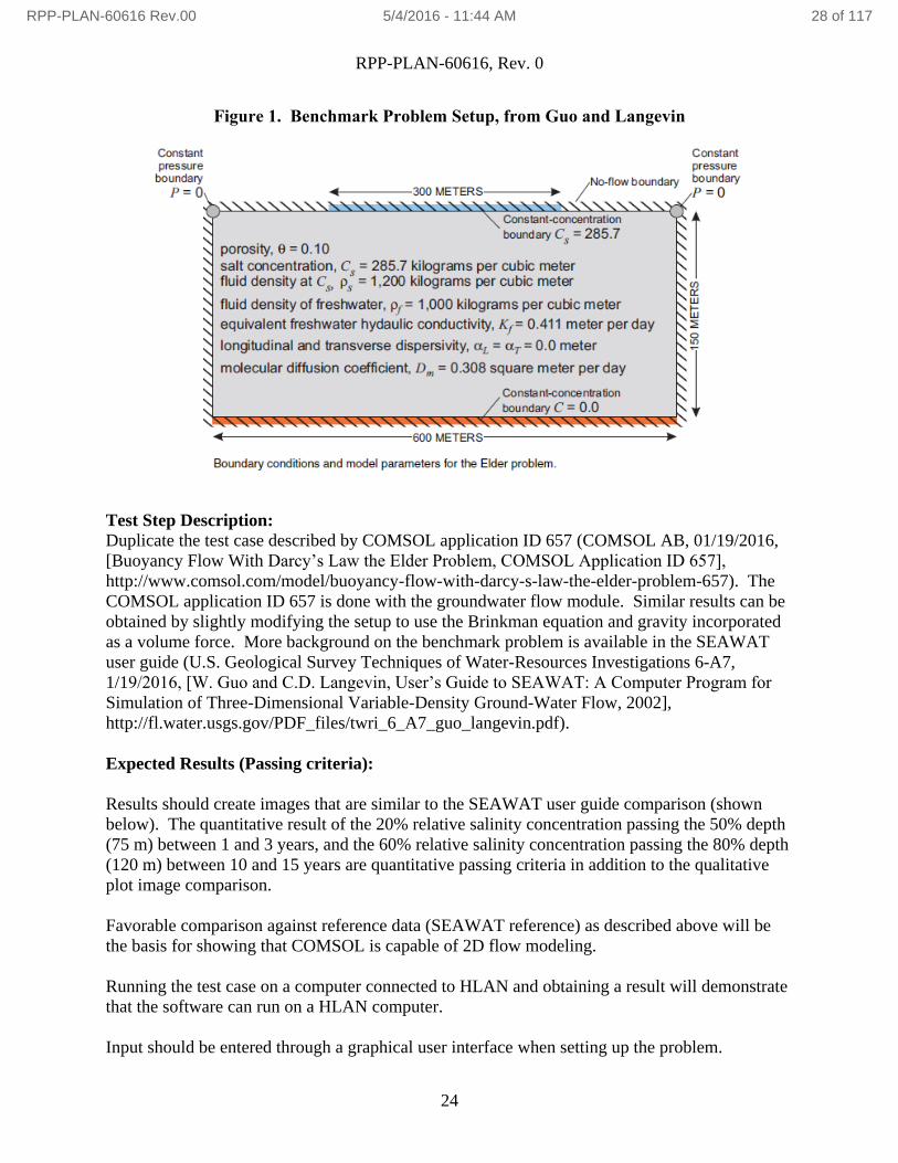
Figure 1. Benchmark Problem Setup, from Guo and Langevin
Test Step Description:
Duplicate the test case described by COMSOL application ID 657 (COMSOL AB, 01/19/2016,
[Buoyancy Flow With Darcy’s Law the Elder Problem, COMSOL Application ID 657],
http://www.comsol.com/model/buoyancy-flow-with-darcy-s-law-the-elder-problem-657). The
COMSOL application ID 657 is done with the groundwater flow module. Similar results can be
obtained by slightly modifying the setup to use the Brinkman equation and gravity incorporated
as a volume force. More background on the benchmark problem is available in the SEAWAT
user guide (U.S. Geological Survey Techniques of Water-Resources Investigations 6-A7,
1/19/2016, [W. Guo and C.D. Langevin, User’s Guide to SEAWAT: A Computer Program for
Simulation of Three-Dimensional Variable-Density Ground-Water Flow, 2002],
http://fl.water.usgs.gov/PDF_files/twri_6_A7_guo_langevin.pdf).
Expected Results (Passing criteria):
Results should create images that are similar to the SEAWAT user guide comparison (shown
below). The quantitative result of the 20% relative salinity concentration passing the 50% depth
(75 m) between 1 and 3 years, and the 60% relative salinity concentration passing the 80% depth
(120 m) between 10 and 15 years are quantitative passing criteria in addition to the qualitative
plot image comparison.
Favorable comparison against reference data (SEAWAT reference) as described above will be
the basis for showing that COMSOL is capable of 2D flow modeling.
Running the test case on a computer connected to HLAN and obtaining a result will demonstrate
that the software can run on a HLAN computer.
Input should be entered through a graphical user interface when setting up the problem.
RPP-PLAN-60616 Rev.00 5/4/2016 - 11:44 AM 28 of 117

RPP-PLAN-60616, Rev. 0
25
The setup data needed to run the program as shown in Figure 1 should be captured in the output
report. The units may need to be manipulated to enter in the form that is most convenient to use
within COMSOL, however the data should be present. A spot check will be done of the porosity
to show it is reported in the output report.
Figure 2. Expected Results for Density Driven Flow in Porous Media (from Guo and
Langevin)
2.9.1.2 Test Case ID: TC-B
Description: Natural convection in square cavity
This problem looks at natural convection within a square cavity using a well document
benchmark problem. The problem is stated in non-dimensional units. It consists of a box of 1
unit length. The left side is cooled to T=0, and the right side is heated to T=1. Flow conditions
of Ra number equal to 103, 104, 105, and 106 are examined.
RPP-PLAN-60616 Rev.00 5/4/2016 - 11:44 AM 29 of 117

RPP-PLAN-60616, Rev. 0
26
Figure 3. Natural Convection Benchmark Notation, from Davis
Test Step Description:
Follow COMSOL application ID: 665 (COMSOL AB, 01/19/2016, [Buoyancy Flow of Free
fluids, COMSOL Application ID: 665], http://www.comsol.com/model/buoyancy-flow-of-free-
fluids-665). More background can be read on this benchmark case in the G. de Vahl Davis paper
(G. de Vahl Davis (G. de Vahl Davis and I.P. Jones, “Natural Convection in a Square Cavity: A
Comparison Exercise,” Int. J. Num. Meth. in Fluids, vol. 3, pp. 227–248, 1983).
Expected Results (Passing criteria):
RPP-PLAN-60616 Rev.00 5/4/2016 - 11:44 AM 30 of 117

RPP-PLAN-60616, Rev. 0
27
The bench mark results from the de Vahl Davis paper are shown in the table. The average Nu
number ( Nu ) should be within 5% of the value presented for the four different Rayleigh
numbers listed.
Table 4. The Bench Mark Solution to Natural Convection in a Square Cavity, from Davis
Rayleigh Number 103 104 105 106
1.118 2.243 4.519 8.800
Qualitatively the results should reflect those presented in the COMSOL application for natural
convection in a square cavity.
Figure 4. Expected Results for Natural Convection in a Square Cavity, from COMSOL
RPP-PLAN-60616 Rev.00 5/4/2016 - 11:44 AM 31 of 117

RPP-PLAN-60616, Rev. 0
28
2.9.1.3 Test Case ID: TC-C
Description: Heat Transfer Test Set
This test case goes through an assortment of heat transfer problems to test COMSOL against
textbook conduction, convection, and radiation problems.
Test Step Description:
This test case will solve a set of heat transfer problems with COMSOL that can be compared
with simple hand calculations.
TC-C-1: Conduction
A conduction text book problem will be solved (from Introduction to Heat Transfer, F.P.
Incropera and D.P. DeWitt, 1996, John Wiley and Sons), Example 1.1 from Incropera and
DeWitt. A brick of 0.15 m thickness, 0.5 m height, and 3 m length is heated to 1400 K on one
side (the 0.5 m by 3 m face), and the opposite side is at 1150 K. The thermal conductivity (k) is
1.7 W/(m K). The heat transfer through the brick is described by Fourier’s law, and gives 2833
W/m^2 or 4250 W for this segment of wall. COMSOL results should be within +/- 5% for heat
transferred at the boundary as calculated with hand calculations below.
Where
k is the thermal conductivity of the solid
dt is the temperature difference across the brick
L is the thickness of the brick
q is the heat flux through the brick per area
qx is the heat transferred by the brick.
RPP-PLAN-60616 Rev.00 5/4/2016 - 11:44 AM 32 of 117

RPP-PLAN-60616, Rev. 0
29
TC-C-2: Heat Generation
Using the geometry described in TC-C-1, the hot (1400K) side boundary will be removed and
replaced with an insulating boundary. The volumetric heat generation term of 5 W/m^3 will be
set for the area. The only place for the heat to go is out the cold boundary, so the heat transferred
at the cold boundary (qHG) should be 1.125 W (+/- 5%).
TC-C-3: Convection Boundary
Using the geometry described in TC-C-1, the cold (1150 K) boundary will be replaced with a
convective heat transfer coefficient of 5 W/m^2*K and an ambient temperature of 300 K will be
used. Heat flux should be described by:
Where
Th is the hot side temperature
Tc is the cold side temperature
h is the convective heat transfer coefficient
A is the area exposed to convective heat transfer
qcon is the convective heat transferred by the brick
The temperature of the convective surface can be found by setting the convective boundary flux
equal to the conductive flux through the brick in this case.
𝑞 = 𝐴 ∗ (𝑇𝐻 − 𝑇𝐶) ∗ ℎ = 𝐴 ∗ 𝑘 ∗ 𝑑𝑡/𝑑𝐿
Variables are as defined above. This gives a temperature expected at the surface of:
𝑇𝐻 =(
𝑘
𝐿)∗1400𝐾+ℎ∗300
(ℎ+𝑘
𝐿)
= 1063.2653 K
Which then gives a heat transfer rate of 5724.49 W
TC-C-4: Convection Calculation
RPP-PLAN-60616 Rev.00 5/4/2016 - 11:44 AM 33 of 117

RPP-PLAN-60616, Rev. 0
30
This problem will solve Example 7.1 from Incropera and DeWitt. A plate of 0.5 m is maintained
at 27 C while air at 300 C and 6 kN/m^2 pressure flow over it at 10 m/s. The heat flux can be
calculated as follows by hand, and the COMSOL result should be within +/- 15% for the heat
flux per length. The uncertainty for this heat transfer coefficient was not explicitly stated in the
Incropera and DeWitt text, however other convective heat transfer coefficients were listed as
having accuracy of 15%, so that was assumed here as well. Properties are given as follows,
kinematic viscosity 5.21x10^-4 m^2/s, thermal conductivity is 0.0364 W/(m K), and the Prandtl
number is 0.687.
Where
Tb is the bulk fluid temperature of air
Ts is the surface temperature of the plate
v is the kinematic viscosity of the fluid
L is the plate length
u is the fluid velocity
k is the thermal conductivity
Pr is the Prandtl number
Re is the Reynolds number
Nu is the Nusselt number
h is the heat transfer coefficient
q’ is the heat delivered to the plate per unit width
RPP-PLAN-60616 Rev.00 5/4/2016 - 11:44 AM 34 of 117

RPP-PLAN-60616, Rev. 0
31
TC-C-5: Porous Media
A rectangle of length 0.5 m and height 0.1 m is insulated on the top and bottom. The left side is
hot at 90 C, and the right side is cold at 40 C. The media of the calculated area is porous, with a
solid fraction of 0.305. The fluid is like water with a thermal conductivity of 0.6 W/m K, and it
is stagnant. The solid is like steel with a thermal conductivity of 50.2 W/m K. The heat flux
should match the hand calculation within +/-5%.
Where
ks is the thermal conductivity of the solid
kl is the thermal conductivity of the liquid
keq is the combined thermal conductivity of the liquid filled porous material
Θ is the solid fraction of the material
dt is the temperature difference across the porous material
L is the length over which heat is transferred
qx is the heat transferred per unit length
There are a number of ways to calculate conductive heat transfer through porous material. The
method employed here is to use a volume average. The volume average model would book end
the upper value for thermal conductivity as it assumes two independent parallel heat transfer
paths based on the void fraction. Other models for porous media conduction are built into
COMSOL (specifically a reciprocal or series resistance model and a power law model). If more
RPP-PLAN-60616 Rev.00 5/4/2016 - 11:44 AM 35 of 117

RPP-PLAN-60616, Rev. 0
32
advanced models for calculating porous media conduction are desired, (such as the Hadley
correlation which has been used in Hanford tank sludge modeling in the past and is described in
PNL-10695, Mahoney, L.A., Trent, D.S., Correlation Models for Waste Tank Sludge and
Slurries, Pacific Northwest Laboratory, July 1995), then those equations can be entered directly
into COMSOL for the mean thermal conductivity.
TC-C-6: Radiative heat transfer
This will follow Example 13.5 from Incropera and DeWitt. A tube flowing cryogenic liquid is
surrounded by a vacuumed line. The geometry can be represented in two dimensions as two
concentric circles creating an annular space. The larger circle is 300K, 50mm in diameter, with
an emissivity of 0.05. The smaller circle is 77 K, 20 mm in diameter, with an emissivity of 0.02.
The wall temperatures are maintained and the space between them is evacuated. Both surfaces
are diffuse and gray. The heat transferred by radiation should match the value calculated within
+/-5%.
Where
D1 is the inner diameter
D2 is the outer diameter
ε1 is the emissivity of the inner surface
ε2 is the emissivity of the outer surface
T1 is the temperature of the inner surface
T2 is the temperature of the outer surface
σ is the Stefan-Boltzmann constant
q’ is the heat flux per unit width
RPP-PLAN-60616 Rev.00 5/4/2016 - 11:44 AM 36 of 117

RPP-PLAN-60616, Rev. 0
33
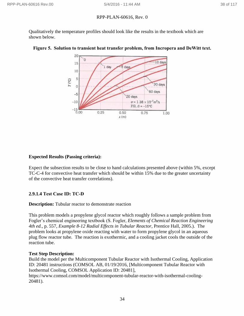
TC-C-7: Transient heat transfer analysis
This will follow Example 5.5 from Incropera and DeWitt looking at the change in temperature
over time of a soil column. Soil with a surface temperature of -15 C, density of 2050 kg/m^3,
thermal conductivity of 0.52 W/(m*K), and heat capacity of 1840 J/(kg*K) is initially at 20 C.
Calculate the depth that is at 0 C at day 60, as well as the temperature profile for time from 1 to
60 days and a depth of 0 to 1 m.
Where
Ti is the initial temperature of the bulk medium
Ts is the surface temperature
Td is the temperature of interest at depth
ρ is the solid density
k is the thermal conductivity of the soil
c is the heat capacity of the soil
α is a parameter that is used to simplify calculations
x is the distance from the surface
t is time
erf() is the error function
sol and find() are calculations in Matlab to solve the function specified.
The depth of 0 C soil at day 60 should be calculated by COMSOL to be within +/- 5% of 0.677
m from the surface.
RPP-PLAN-60616 Rev.00 5/4/2016 - 11:44 AM 37 of 117
RPP-PLAN-60616, Rev. 0
34
Qualitatively the temperature profiles should look like the results in the textbook which are
shown below.
Figure 5. Solution to transient heat transfer problem, from Incropera and DeWitt text.
Expected Results (Passing criteria):
Expect the subsection results to be close to hand calculations presented above (within 5%, except
TC-C-4 for convective heat transfer which should be within 15% due to the greater uncertainty
of the convective heat transfer correlations).
2.9.1.4 Test Case ID: TC-D
Description: Tubular reactor to demonstrate reaction
This problem models a propylene glycol reactor which roughly follows a sample problem from
Fogler’s chemical engineering textbook (S. Fogler, Elements of Chemical Reaction Engineering
4th ed., p. 557, Example 8-12 Radial Effects in Tubular Reactor, Prentice Hall, 2005.). The
problem looks at propylene oxide reacting with water to form propylene glycol in an aqueous
plug flow reactor tube. The reaction is exothermic, and a cooling jacket cools the outside of the
reaction tube.
Test Step Description:
Build the model per the Multicomponent Tubular Reactor with Isothermal Cooling, Application
ID: 20481 instructions (COMSOL AB, 01/19/2016, [Multicomponent Tubular Reactor with
Isothermal Cooling, COMSOL Application ID: 20481],
https://www.comsol.com/model/multicomponent-tubular-reactor-with-isothermal-cooling-
20481).
RPP-PLAN-60616 Rev.00 5/4/2016 - 11:44 AM 38 of 117
RPP-PLAN-60616, Rev. 0
35
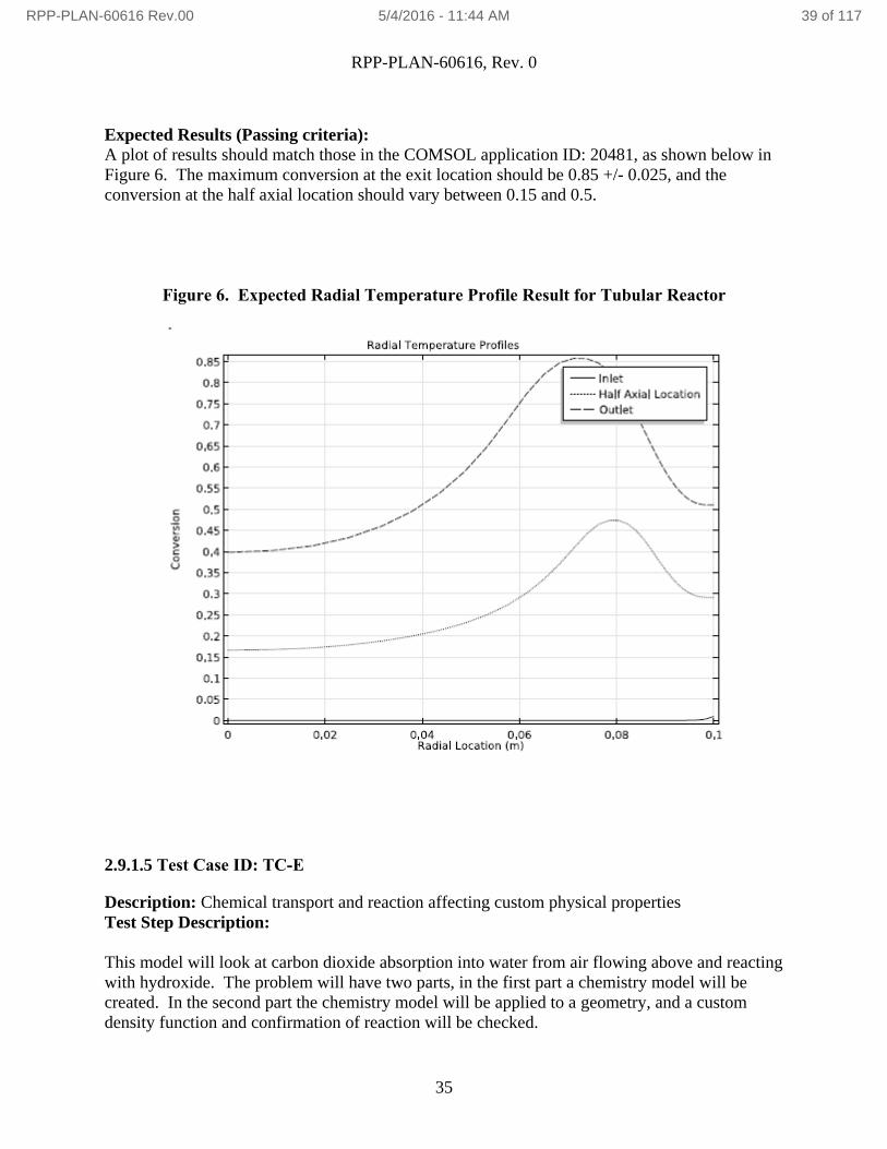
Expected Results (Passing criteria):
A plot of results should match those in the COMSOL application ID: 20481, as shown below in
Figure 6. The maximum conversion at the exit location should be 0.85 +/- 0.025, and the
conversion at the half axial location should vary between 0.15 and 0.5.
Figure 6. Expected Radial Temperature Profile Result for Tubular Reactor
2.9.1.5 Test Case ID: TC-E
Description: Chemical transport and reaction affecting custom physical properties
Test Step Description:
This model will look at carbon dioxide absorption into water from air flowing above and reacting
with hydroxide. The problem will have two parts, in the first part a chemistry model will be
created. In the second part the chemistry model will be applied to a geometry, and a custom
density function and confirmation of reaction will be checked.
RPP-PLAN-60616 Rev.00 5/4/2016 - 11:44 AM 39 of 117

RPP-PLAN-60616, Rev. 0
36
TC-E-1: Chemistry Model
A seawater system will be modeled as an analogous system to the Hanford underground storage
tanks, as carbon dioxide absorption into seawater is a more highly studied system and data is
readily available. The reactions and rate data will come from the Schulz paper (Schulz, K.G., et.
al., Determination of the rate constants for the carbon dioxide to bicarbonate inter-conversion in
pH-buffered seawater systems, Marine Chemistry 100 (2006) 53-65), and the reactions are as
described below (note, the nomenclature from the Schulz paper has been retained):
(1)
(4)
(5 H+)
(5OH-)
(6)
(a)
Where AH is a buffer and A- is the dissociated buffer. To duplicate the results from the Schulz
paper, the buffer HEPES (2-[4-(2-hydroxyethyl)piperazin-1-yl]ethanesulfonic acid) will be used
(pKa=7.59, initial concentration 50 mM, and pH adjusted to 8).
The following rate constants will be used at a temperature of 15 C and a salinity of S=35. Note
that the “Check value” given in the Schulz paper (also as shown in Table 5) is at 298.15 K, not
15 C which is the temperature used in this exercise.
RPP-PLAN-60616 Rev.00 5/4/2016 - 11:44 AM 40 of 117

RPP-PLAN-60616, Rev. 0
37
Table 5. Rate Constants Used In Test Case, from Schulz
Note that COMSOL uses mol/m^3 for concentration units, so the above rate constants need to be
converted from mol/L or mol/kg to mol/m^3. The assumption of a fixed density of 1023 kg/m^3
is made. This is not exactly correct, but should be sufficient. It is close to an average value of
sea water for the first part (Wikipedia gives sea water as having a density between 1020 and
1029 kg/m^3, (Wikipedia, 03/28/2016, [Seawater], https://en.wikipedia.org/wiki/Seawater)). For
the second part where the rate constants are applied to a geometry the accuracy of the rate
constants is less important, so a density deviation of 25% will not adversely impact the final
result.
The system used to generate figure 3-G in the Schulz paper will be duplicated to demonstrate the
chemistry is implemented correctly.
RPP-PLAN-60616 Rev.00 5/4/2016 - 11:44 AM 41 of 117

RPP-PLAN-60616, Rev. 0
38
Figure 7. CO2 Concentration change and other species, from Schultz paper.
TC-E-2
Setup a model with air flowing through the upper section and stagnant liquid below. The model
geometry is roughly shown . The liquid region will have a hydroxide concentration gradient
from 0 on the left side to 16 mol/l on the right side. The air will blow from left to right at a
speed of 1 ft/min with a concentration of 350 ppm CO2. The geometry dimensions for the box
are 1 meter wide, 0.5 m height liquid region, and 0.1 m high gas region above the liquid (laminar
flow is assumed so the gas region does not need to be very thick). The air enters at 300 K, and
the system initially has a temperature gradient from 280 K at the bottom to 360 K at the top of
the liquid surface. The purpose of the gradients is to provide different combinations of
temperature and concentration to check the density calculation against.
RPP-PLAN-60616 Rev.00 5/4/2016 - 11:44 AM 42 of 117
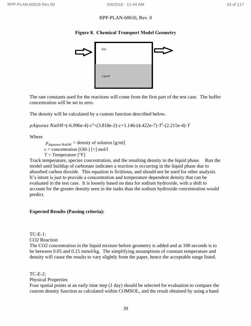
RPP-PLAN-60616, Rev. 0
39
Figure 8. Chemical Transport Model Geometry
The rate constants used for the reactions will come from the first part of the test case. The buffer
concentration will be set to zero.
The density will be calculated by a custom function described below.
𝜌𝐴𝑞𝑢𝑜𝑢𝑠 𝑁𝑎𝑂𝐻=(-6.096e-4)·c2+(3.818e-2)·c+1.146-(4.422e-7)·T2-(2.215e-4)·T
Where
𝜌𝐴𝑞𝑢𝑜𝑢𝑠 𝑁𝑎𝑂𝐻 = density of solution [g/ml]
c = concentration [OH-] [=] mol/l
T = Temperature [°F]
Track temperature, species concentration, and the resulting density in the liquid phase. Run the
model until buildup of carbonate indicates a reaction is occurring in the liquid phase due to
absorbed carbon dioxide. This equation is fictitious, and should not be used for other analysis.
It’s intent is just to provide a concentration and temperature dependent density that can be
evaluated in the test case. It is loosely based on data for sodium hydroxide, with a shift to
account for the greater density seen in the tanks than the sodium hydroxide concentration would
predict.
Expected Results (Passing criteria):
TC-E-1:
CO2 Reaction
The CO2 concentration in the liquid mixture before geometry is added and at 100 seconds is to
be between 0.05 and 0.15 mmol/kg. The simplifying assumptions of constant temperature and
density will cause the results to vary slightly from the paper, hence the acceptable range listed.
TC-E-2:
Physical Properties
Four spatial points at an early time step (1 day) should be selected for evaluation to compare the
custom density function as calculated within COMSOL, and the result obtained by using a hand
RPP-PLAN-60616 Rev.00 5/4/2016 - 11:44 AM 43 of 117

RPP-PLAN-60616, Rev. 0
40
calculation with the same function given the temperature and concentration values found. The
four points should represent a spread of values of temperature and concentration. The density
should match hand calculations within 5% for the temperature and concentration given.
Reaction
The carbonate concentration, as the terminal reaction product for the carbon dioxide reaction,
should increase by more than 1000 mol/m^3 at the surface at the point of maximum
concentration at the end of one year. Qualitatively the hydroxide concentration should decrease
near the surface in the same region.
Evidence that CO2 is diffusing across the interface and reacting , such as buildup of reaction
products over time. This will be a qualitative observation.
2.9.1.6 Test Case ID: TC-F
Description: Fluid flow velocity profile
Test Step Description:
Flow in a confined annulus (such as a pipe) has an analytically well-defined velocity profile.
This model will test COMSOL’s ability to reproduce the velocity profile.
Setup a 3D tube of 0.5 in radius, 10 ft length, 20 psia inlet pressure, and 19.9 psia outlet pressure
and a viscosity of 1 poise and determine the velocity profile in the pipe. The modeled test length
can be changed but the pressure gradient (0.01 psi/ft) should remain the same as that will
establish the velocity profile.
Expected Results (Passing criteria):
TC-F-1:
The fully developed laminar velocity profile is given in text (Transport Phenomena, R.B. Bird,
W.E. Stewart, and E.N. Lightfoot, 1960, John Wiley and Sons) as:
RPP-PLAN-60616 Rev.00 5/4/2016 - 11:44 AM 44 of 117

RPP-PLAN-60616, Rev. 0
41
Where:
Po is the inlet pressure
Pl is the outlet pressure
R is the radius
r is the axial location the velocity is calculated at
µ is the viscosity
L is the length of the pipe
The model value should match a velocity of 0.299 ft/sec +/- 10% when calculated at the
centerline (r=0).
The model will be run in 3D, and achieving passing velocity results will also be passing criteria
for the 3D model run.
Unit conversion will be tested by entering the geometry in feet and inches, fluid properties in SI
units, pressure in psi, then outputting the maximum velocity results in both m/s and ft/s to ensure
the values match (within 2%).
TC-F-2
The fully developed laminar flow velocity profile should qualitatively look similar to the figure
below.
RPP-PLAN-60616 Rev.00 5/4/2016 - 11:44 AM 45 of 117

RPP-PLAN-60616, Rev. 0
42
Figure 9. Fully Developed Laminar Flow Velocity Profile
Additionally, if a constant velocity inlet is used, the flow profile should develop similar to the
figure below, this will be a qualitative evaluation of similarity. If a pressure boundary is used the
profile should enter somewhat developed and their will not be the constant velocity across the
diameter on the inlet.
Figure 10. Example of Flow Development
(Wikipedia, 03/28/2016, [Entrance length], https://en.wikipedia.org/wiki/Entrance_length.)
RPP-PLAN-60616 Rev.00 5/4/2016 - 11:44 AM 46 of 117

RPP-PLAN-60616, Rev. 0
43
2.9.1.7 Test Case ID: TC-G
Description: Diffusion Test
Test Step Description:
A simple diffusion tube will be looked at to study transient diffusion. The solution can be
analytically computed providing a definitive comparison with the COMSOL results.
The geometry will be a rectangle with 0.1 m width and 1 m height. The rectangle will be filled
with stagnant water and CO2 at a concentration of 0.001 g/kg. The upper boundary of the
rectangle will have CO2 at a concentration of 0.5 g/kg CO2. The region 5 cm below the surface
should see a rise in CO2 that is described by Fick’s second law shown below.
Where
C’ is the difference between initial concentration and concentration at time t at a point y
CA is the species concentration at time t and location y
CA0 is the initial species concentration at time t=0 in the bulk
CAi is the initial concentrated species at the reference plane (concentrated location at y=0)
y is the distance from the reference plane
t is the time
erfc() is the complementary error function
D is the diffusivity
Equation is from:
Coulson, J.M. Richardson, J.F. Backhurst, J.R. Harker, J.H.. (1999). Coulson and Richardson's
Chemical Engineering Volume 1 - Fluid Flow, Heat Transfer and Mass Transfer (6th Edition),
Elsevier.
Also from the above reference, the diffusivity of CO2 in water is D=1.5x10^-9 m^2/s, and this
value will be entered into COMSOL.
RPP-PLAN-60616 Rev.00 5/4/2016 - 11:44 AM 47 of 117

RPP-PLAN-60616, Rev. 0
44
Expected Results (Passing criteria):
Concentration at the given depth should be within +/-5% of full value (0.025 g/kg). Values less
than 5% of the maximum concentration value are too close to zero for a relative error to be
meaningful.
2.9.1.8 Test Case ID: TC-H
Description: Jet Mixing
Test Step Description:
This set of test problems will evaluate COMSOL’s ability to run jet mixing problems.
TC-H-1: Neutrally Buoyant Jet in Water
This subcase will look at a neutrally buoyant turbulent jet where there are no density differences
between the bulk fluid and the jet. The jet fluid and ambient fluid will be the same density, and
have the properties of water at 300K. The jet entrance radius is 0.2 m, with a concentration of 1
g/m^3 solute. Blevins gives a correlation for centerline velocity and concentration at distance
“x” from the nozzle entrance (table 9-3 in Blevins). A distance of 4 meters will be examined
with the correlations presented by Blevins.
RPP-PLAN-60616 Rev.00 5/4/2016 - 11:44 AM 48 of 117

RPP-PLAN-60616, Rev. 0
45
Where:
r0 is the entrance nozzle radius
x is the centerline distance from the nozzle entrance
U0 is the velocity at the nozzle entrance
um is the centerline velocity at distance x
dT0 is the concentration at the nozzle entrance
dTm is the concentration at the centerline at distance x from the nozzle
The velocity and concentrations calculated are expected to be within 10% of the values
determined with the hand calculation, per the accuracy reported by Blevins. The jet mixing
solutions are more empirical in nature and thus there is more uncertainty then some of the other
test cases.
TC-H-2: Negatively Buoyant Downward Forced Jet
This test case will look at a negatively buoyant (jet fluid is more dense then bulk fluid) turbulent
jet injected downwards. The problem is analogous to a positively buoyant (jet fluid is less dense
than bulk fluid) jet injected upwards. A reservoir of water (density 1000 kg/m^3) will have a
turbulent jet enter from the top pointed downward with a density that is greater (1200 kg/m^3)
than the water. Physical properties other than density are assumed to be the same as water. The
nozzle is 0.06 m radius and flowing at 0.8 m/s. Blevins gives the equations for such a system as
shown below:
RPP-PLAN-60616 Rev.00 5/4/2016 - 11:44 AM 49 of 117

RPP-PLAN-60616, Rev. 0
46
Where:
u is the entrance velocity
r0 is the radius of the entrance nozzle
Q0 is the entrance volumetric flow rate at the nozzle entrance
rho_0 is the fluid injected density
rho_a is the ambient density
g is the acceleration due to gravity
B is the specific buoyancy flux
um is the centerline velocity of the forced plume at distance x from the nozzle
dTm is the concentration at the centerline of the forced plume at distance x from the
nozzle. dT0 is 1 g/m^3.
RPP-PLAN-60616 Rev.00 5/4/2016 - 11:44 AM 50 of 117

RPP-PLAN-60616, Rev. 0
47
v is the kinematic viscosity
Re is the Reynolds number (used to check validity of equation by ensuring over 4000)
The velocity and concentration calculated should match simulation results within 20%. While
Blevins reports a 10% uncertainty in the equations he presents, the greater of the two correlations
in Wigel are 28% different from Blevins, thus a 20% uncertainty is used. The jet mixing
solutions are more empirical in nature and thus there is more uncertainty then some of the other
test cases.
TC-H-3: Positively Buoyant Downward Forced Jet
This subcase will look at a less dense liquid (water, density 1000 kg/m^3) falling upon a more
dense liquid such as water with caustic in it (density 1200 kg/m^3. Using a geometry where the
nozzle entering at the top is pointing down, the maximum jet penetration depth can be calculated.
A circular nozzle of 0.3 m radius was used with 1 m/s velocity. Blevins provides a formula (9-
58) for a negatively buoyant jet, and this can be used by analogy for a positively buoyant jet as
shown below:
Where the variables are as described in the previous test case with the addition of the following:
M is the momentum flux
a is an empirically derived constant, provided by Blevins as usually around 1.95
xmax is the maximum depth of jet penetration before the plume will fall back on itself.
RPP-PLAN-60616 Rev.00 5/4/2016 - 11:44 AM 51 of 117

RPP-PLAN-60616, Rev. 0
48
The penetration depth should be similar in COMSOL. No accuracy is stated with the formula
presented by Blevins, and the passing criteria is a value with COMSOL found that will be within
50% of the value provided by Blevins. No uncertainty is reported for the maximum penetration
depth in Blevins. The main interest to tank mixing problems is that the jet turns and creates a
layer, so the penetration depth is less important and a 50% variation is acceptable in the exact
depth of the jet. If future problems require greater accuracy it can be revisited.
Expected Results (Passing criteria):
COMSOL results that match the analytical solutions based on correlations found in the Blevins
text. The acceptable uncertainty and values to match are stated with each sub-case.
2.9.1.9 Test Case ID: TC-I
Description: CO2 Absorption Efficiency
Test Step Description:
This test case will look at headspace gas flow and carbon dioxide transfer to a surface to test the
mass balance ability for chemical species tracking problems. The results will also be compared
the results with what might be expected based on past observations. D.T. Hobbs did a study of
carbon dioxide absorption efficiency in waste storage tanks, and that will be used as reference.
The model geometry will be a simplification of the headspace (air volume only) geometry of a
double shell tank:
75’ Diameter cylinder with flat bottom
15’ cylinder height (possible vapor space in a tank, liquid excluded from the model)
Elliptical dome on head with a center height 12’ above the top of the cylinder
Two risers, each 1’ diameter, positioned 40’ apart, each 20’ from the tank centerline
RPP-PLAN-60616 Rev.00 5/4/2016 - 11:44 AM 52 of 117

RPP-PLAN-60616, Rev. 0
49
Figure 11. Geometry of Carbon Dioxide Absorption Efficiency Test Case
One riser is set for inflow with a velocity of 360 ft/min and a concentration of 0.0156 mol/m^3
CO2 (which is near 350 ppm). The other riser is set for outflow with the pressure at atmospheric
(1 atm).
To calculate the CO2 concentration on the air side of the air/liquid interface, a methodology from
RPP-50654 will be employed. The liquid phase CO2 concentration is given by:
[CO2]𝐿𝑖𝑞𝑢𝑖𝑑 =[CO3
2−]
[𝑂𝐻−]∗𝐾𝐶𝑂2∗𝐾𝐻𝐶𝑂3
Where:
[CO32-]=0.05 M
[OH-]=0.1 M
KCO2=3.54e7
KHCO3=4.63e3
So that
[CO2]Liquid=3.05e-11 M
The air across the interface can be described by Henry’s law
PCO2=Hc*[CO2]Liquid
Where:
PCO2 is the partial pressure of carbon dioxide in mmHg
Hc=1 mmHg/4.48e-5 (mol/L), Henry’s constant for CO2 in water
RPP-PLAN-60616 Rev.00 5/4/2016 - 11:44 AM 53 of 117
RPP-PLAN-60616, Rev. 0
50
So that assuming a temperature of 300K and a pressure of 1 bar, the molar concentration of
carbon dioxide in air in equilibrium with the liquid below is 3.630e-8 mol/m^3.
Expected Results (Passing criteria):
TC-E-1: Conservation of mass transport
The flux of CO2 entering the inlet riser should equal the flux at the outlet riser plus the flux at
the bottom surface. This value represents a mass balance of CO2 around the tank assuming no
accumulation or generation at steady state.
The sum of the CO2 exiting the tank should be within +/- 10% of the value entering.
TC-E-2: CO2 Absorption
D.T. Hobbs in report DST-87-596 gives an empirical correlation for CO2 absorption in a waste
tank the surface of a tank. He defines an absorption fraction as:
𝐴𝑏𝑠𝑜𝑟𝑝𝑡𝑖𝑜𝑛 𝐹𝑟𝑎𝑐𝑡𝑖𝑜𝑛 =([𝐶𝑂2]𝑒𝑛𝑡𝑒𝑟 − [𝐶𝑂2]𝑒𝑥𝑖𝑡)
[𝐶𝑂2]𝑒𝑛𝑡𝑒𝑟
The absorption fraction ranges from 0.096 to 0.843 in the tanks studied and was found to most
strongly correlate with pH. Hobbs presents a formula for the absorption fraction as a function of
pH
Absorption Fraction = 0.165*pH-1.569
For a hydroxide concentration of 0.1 M, assuming pH+pOH=14, the pH of the solution must be
13. This corresponds to an expected absorption fraction of 0.55.
Built into the Hobbs correlation are a number of variables specific to the Savannah river tanks
the correlation came from. For instance ventilation flow rate, temperature difference, ambient
temperatures, and waste transport properties are all know to be important to carbon dioxide
absorption but are not part of the equation given by Hobbs. Additionally this problem simplifies
the analysis by trying to omit the liquid phase mass transport by assuming a well-mixed tank and
no boundary layer to diffusion on the liquid side. This may or may not be a good assumption.
Thus it is difficult to predict how much uncertainty will exist with the Hobbs equation.
The absorption fraction found with COMSOL will be reported and compared with the Hobbs
equation, however passing values are anything between 0.01 and 0.99.
RPP-PLAN-60616 Rev.00 5/4/2016 - 11:44 AM 54 of 117

RPP-PLAN-60616, Rev. 0
51
2.9.1.10 Test Case ID: TC-J
Description: Water Evaporation and Level Change
Test Step Description:
This test case will look at mass transfer of water at an air/liquid interface. A small volume of
water is present, and when looking at level change air is blowing over it. The simulation should
track the water evaporation to capture the phase change from the liquid to gas phase, and the
interface position between the gas and liquid should move based on the loss of water vapor from
the liquid phase. A simple geometry, that of a trench, will be used. Liquid water initially at 80
F (300 K) will be used. Air flowing over it is at 116 F (320 K). The sides of the trench have a
convective boundary with a convective heat transfer coefficient of 1000 W/(m^2*K) and an
external temperature of 293.15 K. The air velocity over the surface is 1 m/s. The geometry is
described in the figure below. The first part of the problem will look at diffusion only with no
gas flow to see if the water/air interface is being simulated correctly. The second part will
consider the gas flowing over the surface to cause a level change in the liquid.
Figure 12. Geometry for TC-J
It is assumed that water is in equilibrium with the gas above it.
Expected Results (Passing criteria):
TC-J-1: Water Evaporation into gas
Water at 80 F should have a vapor pressure of 0.03581 bar (National Institute of Standards and
Technology, 3/28/2016, [Water],
http://webbook.nist.gov/cgi/cbook.cgi?ID=C7732185&Units=SI&Mask=4#Thermo-Phase), or
0.5193 psi, or 3580 Pa . System pressure is near atmospheric, of 14.7 psia, so the volume
fraction should be about 3.5% water in the air immediately above the liquid surface on the
RPP-PLAN-60616 Rev.00 5/4/2016 - 11:44 AM 55 of 117

RPP-PLAN-60616, Rev. 0
52
downstream side. Passing criteria then is a water volume fraction of 3.5% (+/- 10%) in the air
immediately above the liquid surface on the downstream side is passing. If the temperature of
the liquid surface changes from 80F, the vapor pressure at the actual temperature in the model
should be used to obtain the vapor pressure and re-calculate what the expected water volume
fraction should be. COMSOL gives concentration in mol/m^3, so 0.5193 psi corresponds to 1.44
mol/m^3 (0.5193 psi is 3580 Pa, mol/m^3=3580Pa/(300K*8.31446 m^3*Pa/(K*mol))).
TC-J-2: Water Level
The water level should decrease as the water evaporates. The water evaporated will be
calculated by measuring the mass flux of water leaving the outlet boundary. The water level
should decrease by an amount equal to the mass lost. The calculated level change as estimated
by the water mass lost should match the water level in the simulation within +/-10%.
The mass of water should be conserved in the system. This will be calculated by:
Total water mass change in the liquid system=Mass of water entering gas phase
The liquid water volume change and the mass of water that has entered the gas phase should be
within +/- 5% of each other.
RPP-PLAN-60616 Rev.00 5/4/2016 - 11:44 AM 56 of 117

RPP-PLAN-60616, Rev. 0
53
2.10 RETIREMENT PLAN/CHECKLIST
No plans for retirement at this time. A Retirement Plan will be developed under TFC-BSM-
IRM_HS-C-01 prior to retirement of this software.
2.11 ACQUISITION
Software is sold a developed package, and is simply purchased from the vendor by a WRPS
buyer. The ADP form # 2015-10-ADP0100 has vendor details.
The software evaluation plan includes the following:
1. Capabilities and limitations for intended use: Refer to Section 2.2
2. Test Plan and Test cases as method of acceptance: Refer to Section 2.9
Approval of this SMP with the completed Acceptance Testing (See Section 2.19) constitutes
acceptance of the software.
2.11.1 Error Reporting
With an active license of COMSOL, WRPS is able to participate in the subscription program for
updates. This alerts users if new updates to the program are available, and allows them to
download the version and related license files. The software owner will maintain a subscription
to the COMSOL update feed. Any changes to the Configuration Items specified in 2.6 will
adhere to Section 2.6.4 Configuration Change Control.
If WRPS finds a problem in the software, it can be reported to COMSOL and the vendor may
send it to their development team to resolve in the next software release. WRPS would need to
evaluate the extent of the problem, and act accordingly. This may involve a PER process
described in TFC-ESHQ-Q_C-C-01 if appropriate.
2.12 SOFTWARE DESIGN
Software Design is not applicable to Acquired software.
2.13 UNIT AND SYSTEM TESTING
Unit are not applicable to Acquired software. System Testing requirements are addressed
through testing of the Software Requirement in Section 2.7 and executing of the Acceptance Test
Plan in Section 2.9.
2.14 TECHNICAL AND PEER REVIEWS
RPP-PLAN-60616 Rev.00 5/4/2016 - 11:44 AM 57 of 117

RPP-PLAN-60616, Rev. 0
54
An independent technical review will be done for the software requirements as part of the
software management plan review cycle. See section 1.10.1.
A review must be done to ensure the quality of a simulation. A user review may be sufficient for
models that are considered “casual use” and not for customer use. If the simulation employs
physics and a structure that fall within the scope of the software management plan, the test case
execution in the software management plant is sufficient for verification. Modes that are not
within the scope of the software management plan (i.e. using model features that are not captured
and tested in the specific requirements) require further validation work that must be completed
and presented with the model results. Simulations built for customer use should follow an
applicable engineering procedure, such as TFC-ENG-DESIGN-C-10, and have a commensurate
review (TFC-ENG-DESIGN-C-52).
A tiered approach is used for the review cycle and quality control. This is to facilitate an easily
scaled approach to using the software. Problems that are more important require a much greater
effort to ensure the quality of the results. The user is responsible for determining the appropriate
level of review for a simulation, and the reviewer for a model is responsible for checking the
approach used.
2.15 SOFTWARE INSTALLATION PLAN
The software will be installed on a single local machine in accordance with TFC-BSM-IRM_HS-
C-09. The machine will be managed by Process Engineering as described in Section 1.5.
2.16 USER QUALIFICATION
User qualification is not required for Level D Acquired software. There are no qualifications for
using COMSOL beyond what would be required to work as a technical staff member at WRPS.
2.17 USER TRAINING
User training is not required for Level D Acquired software.
COMSOL has offered a free half-day introductory workshop in Seattle, WA and Richland, WA
in the past, and that is a recommended introduction to the software if it is possible to attend.
Contact a COMSOL representative for a schedule and to register for a workshop. COMSOL
also offers more in depth training which would be very useful but is not necessary. There are no
plans to control who is using the software. Tracking of the training completed is not required.
2.18 USER DOCUMENTS
The COMSOL web site (http://www.comsol.com/) provides vendor supplied documents if
needed. The user guides can also be included with the software installation if that option is
RPP-PLAN-60616 Rev.00 5/4/2016 - 11:44 AM 58 of 117

RPP-PLAN-60616, Rev. 0
55
selected. At this time, there is no plan or defined need to maintain local copies (physical or
electronic) of the vendor supplied documentation.
2.19 ACCEPTANCE TEST REPORT
Appendix B describes the test cases used for acceptance testing. The test cases were run
between January and April of 2016 by Ryan M. Murray, and then reviewed by John L. Mills.
All of the test cases passed, meeting the needs of the specific requirements as correlated in
Appendix A, “Requirements Traceability Matrix”. Observations of unexpected results and their
dispositions are described in the “Comments” section of each test case in Appendix B, “Test
Case Execution Record”. The “Comments” section describes any model setup changes needed
to resolve unexpected results.
Completion of testing and the resulting evaluation demonstrates this software is acceptable for
use.
2.20 IN-USE TESTS
In use tests for COMSOL will involve running test case TC-D, the tubular reactor. This test case
is chosen because it involves chemical reactions, chemical species transport, heat transfer, and
fluid flow. By touching on a number of different physics with a single well documented
problem, gross issues with the software should be apparent.
In-use testing is to be done whenever the COMSOL software is updated with a minor revision
change, before being run on a new computer, or when the operating system of the installed
computer is updated (for instance from Windows 7 to Windows 10). The in-use test will be run
biennially at a maximum interval, if none of the above have occurred that require an in-use test
be run before then.
In-use test cases are stored in SmartPlant in the directory for the software management plan by
attaching the completed test cases to a revision of the SMP in SPF. Note: By attaching the test
results in SPF the results will be entered into IDMS as a record as required even if not including
the attachments in ‘Record PDF’.
The in use test results must include:
Computer program tested including version identifier
Computer hardware tested
Test equipment and calibrations, where applicable
Date of test
Tester or data recorder
Acceptability.
RPP-PLAN-60616 Rev.00 5/4/2016 - 11:44 AM 59 of 117
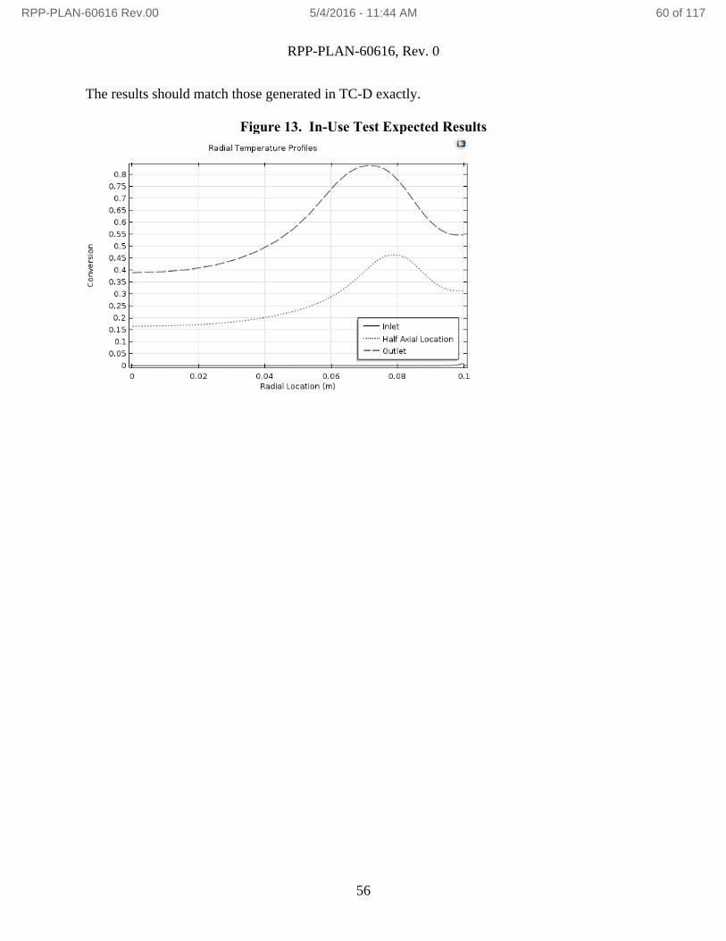
RPP-PLAN-60616, Rev. 0
56
The results should match those generated in TC-D exactly.
Figure 13. In-Use Test Expected Results
RPP-PLAN-60616 Rev.00 5/4/2016 - 11:44 AM 60 of 117

RPP-PLAN-60616, Rev. 0
57
3.0 REFERENCES
Anderson et. al., October 1973, “Negatively Buoyant Jets In A Cross Flow”, EPA-660/2-
73-012US EPA, Corvallis, OR.
Bird, R.B., Stewart, W.E., and Lightfoot, E.N., 1960, Transport Phenomena, John Wiley
and Sons, New York, NY.
Blevins, R.D., 2003, Applied Fluid Dynamics Handbook, Krieger Publishing Company,
Malabar, FL.
COMSOL AB, 03/28/2016, [Finite Element Mesh Refinement, multiphysics cyclopedia],
http://www.comsol.com/multiphysics/mesh-refinement.
COMSOL AB, 03/28/2016, [Nine, B., How to Implement a Mesh Refinement Study,
08/6/13], https://www.comsol.com/blogs/how-to-implement-mesh-refinement-study/.
COMSOL Blog, 03/28/2016, [Frei, W., Which Turbulence Model Should I Choose for
My CFD Application?, 09/16/13], http://www.comsol.com/blogs/which-turbulence-
model-should-choose-cfd-application/.
COMSOL AB, 03/28/2016, [Tubular Reactor With Nonisothermal Cooling Jacket,
Application ID 67], http://www.comsol.com/model/tubular-reactor-with-nonisothermal-
cooling-jacket-67.
COMSOL AB, 01/19/2016, [Buoyancy Flow of Free fluids, COMSOL Application ID:
665], http://www.comsol.com/model/buoyancy-flow-of-free-fluids-665.
COMSOL AB, 01/19/2016, [Buoyancy Flow With Darcy’s Law the Elder Problem,
COMSOL Application ID 657], http://www.comsol.com/model/buoyancy-flow-with-
darcy-s-law-the-elder-problem-657.
COMSOL AB, 03/28/2016, [Smoothed step transitions in COMSOL Multiphysics,
Solution Number 905], http://www.comsol.com/support/knowledgebase/905/.
COMSOL AB, 03/28/16, [Avoiding negative concentrations, Solution Number 952],
https://www.comsol.com/support/knowledgebase/952/.
COMSOL Blog, 03/28/2016, [My flux calculation seems wrong, Solution number 973],
https://www.comsol.com/support/knowledgebase/973/.
COMSOL AB, 03/28/2016, [Solving time dependent CFD simulations, Solution Number
1172], https://www.comsol.com/support/knowledgebase/1172/.
RPP-PLAN-60616 Rev.00 5/4/2016 - 11:44 AM 61 of 117
RPP-PLAN-60616, Rev. 0
58
COMSOL AB, 01/19/2016, [Multicomponent Tubular Reactor with Isothermal Cooling,
COMSOL Application ID: 20481], https://www.comsol.com/model/multicomponent-
tubular-reactor-with-isothermal-cooling-20481.
Coulson, J.M., Richardson, J.F., Backhurst, J.R., Harker, J.H., 1999, Coulson and
Richardson's Chemical Engineering Volume 1 - Fluid Flow, Heat Transfer and Mass
Transfer (6th Edition), Elsevier, Atlanta, GA.
Davis, G. de Vahl, Jones, I.P., 1983, “Natural Convection in a Square Cavity: A
Comparison Exercise,” Int. J. Num. Meth. in Fluids, vol. 3, pp. 227–248.
Fogler, S., 2005, Elements of Chemical Reaction Engineering 4th ed., p. 557, Example 8-
12 Radial Effects in Tubular Reactor, Prentice Hall, Upper Saddle River, NJ.
Hobbs, D.T., September 1987, “Absorption of Carbon Dioxide in Waste Tanks”, DST-
87-596, Westinghouse Savannah River Company, Savannah River, GA
Incropera, F.P., DeWitt, D.P., 1992, Introduction to Heat Transfer, John Wiley and Sons,
New York, NY
LA-14167-MS, Thacker, B. H., et. al., October 2004, “Concepts of Model Verification
and Validation”, Los Alamos National Laboratory, Los Alamos, NM.
National Institute of Standards and Technology, 3/28/2016, [Water],
http://webbook.nist.gov/cgi/cbook.cgi?ID=C7732185&Units=SI&Mask=4#Thermo-
Phase.
Nuclear Energy Agency of the OECD (NEA): Organization for Economic Co-Operation
and Development - Nuclear Energy Agency, 03/28/2016, [Wilkening, H., Baraldi, D., &
Heitsch, M., On the importance of validation when using commercial CFD codes in
nuclear reactor safety, 2007],
https://www.researchgate.net/publication/255580084_ON_THE_IMPORTANCE_OF_V
ALIDATION_WHEN_USING_COMMERCIAL_CFD_CODES_IN_NUCLEAR_REAC
TOR_SAFETY.
PNL-10695, Mahoney, L.A., Trent, D.S., July 1995, “Correlation Models for Waste Tank
Sludges and Slurries”, Pacific Northwest Laboratory, Richland, WA.
RPP-27195, TFC-BSM-IRM_HS-C-01, Rev H, “Software Development,
Implementation, and Management”, Washington River Protection Solutions, LLC,
Richland, WA.
RPP-27195, TFC-BSM-IRM_HS-C-03, Rev E-1, “Software Management”, Washington
River Protection Solutions, LLC, Richland, WA.
RPP-PLAN-60616 Rev.00 5/4/2016 - 11:44 AM 62 of 117
RPP-PLAN-60616, Rev. 0
59
RPP-27195, TFC-ESHQ-Q_C-C-01, Rev K-8, “Problem Evaluation Request”,
Washington River Protection Solutions, LLC, Richland, WA.
RPP-50654, Rev. 0, Powell, W.J., Rosenkrance, C.L, August 2012, “Supernatant
Chemistry Evaluation Model”, Washington River Protection Solutions, LLC, Richland,
WA.
RPP-RPT-58965, Rev 0, “Computational Fluid Dynamic Modeling Software Comparison
for Hanford Tank Simulations”, Washington River Protection Solutions, LLC, Richland,
WA.
RPP-7795, Rev. 13, “Technical Basis for the Chemistry Control Program”, Washington
River Protection Solutions, LLC, Richland, WA.
SAND2003-3769, Oberkampf, W. L., et. al., February 2003, “Verification, Validation,
and Predictive Capability in Computational Engineering and Physics”, Sandia National
Laboratories, Albuquerque, NM.
Santos, R.G., Figueiredo, J.R., July/Sept. 2007, “Laminar elliptic flow in the entrance
region of tubes”, J. Braz. Soc. Mech. Sci. & Eng. vol.29 no.3, Rio de Janeiro. Accessed
on 2/10/2016, http://dx.doi.org/10.1590/S1678-58782007000300001
Schulz, K.G., et. al., Determination of the rate constants for the carbon dioxide to
bicarbonate inter-conversion in pH-buffered seawater systems, Marine Chemistry 100
(2006) 53-65.
Science and Technology of Nuclear Installations, Volume 2009, 03/28/2016, [Xiao, J.,
Travis, J.R., Breitung, W., “Non-Boussinesq Integral Model for Horizontal Turbulent
Buoyant Round Jets,” 2009], http://www.hindawi.com/journals/stni/2009/862934/
TFC-BSM-IR_HS-C-03 Rev E-1, “Software Management, Washington River Protection
Solutions, LLC, Richland, WA
TFC-ENG-DESIGN-C-10, “Engineering Calculations”, Washington River Protection
Solutions, LLC, Richland, WA
TFC-ENG-DESIGN-C-52, “Technical Reviews”, Washington River Protection
Solutions, LLC, Richland, WA
Wiegel, R. L., 1992, Oceanographical Engineering, Prentice-Hall, Englewood Cliffs, N.J.
RPP-PLAN-60616 Rev.00 5/4/2016 - 11:44 AM 63 of 117

RPP-PLAN-60616, Rev. 0
A-1
APPENDIX A
REQUIREMENTS TRACEABILITY MATRIX5
FRD
ID#
Functional Requirement
summary
SRS ID# Specific Requirement
Summary
Test
Case ID#
FR-1 Track the time evolution
of flow through porous
media driven by density
differences given the
necessary boundary
conditions and field
properties.
SR-0.1 Runs on HLAN (Windows
operating system)
TC-A
SR-0.2 Program can convert units
appropriately
TC-F
SR-0.3 Software is interfaced primarily
through a graphical user interface
(GUI)
TC-A
SR-1.1 Can model dense liquid
permeation into porous media
TC-A
SR-1.3 Calculate heat transfer through
porous media
TC-C-5
FR-2 Model the natural
convection of liquid
(calculate fluid
movement driven by
density differences based
on temperature given the
appropriate boundary and
material properties).
SR-2.1 Model natural convection
(calculate fluid movement
resulting from temperature
driven buoyancy differences)
TC-B
SR-2.2 Use a convective boundary to
calculate heat flux
TC-C-3
SR-2.3 Use a calculated convective heat
transfer coefficient to determine
the heat flux
TC-C-4
FR-3 Track chemical species
movement and diffusion
through a fluid system
given appropriate
boundary and material
properties.
SR-1.2 Allow for customization of
physical properties based on
chemical composition and
temperature without the use of an
added library.
TC-E-2
SR-3.1 Capable of chemical species
tracking in 3D including
diffusion, convection, and
absorption mechanisms.
TC-I
SR-3.2 Calculate transient mass transfer
by diffusion
TC-G
5 Only sections relevant to commercial off the shelf software have been included. The design description column
has been omitted because the software was not developed by or for us specifically.
RPP-PLAN-60616 Rev.00 5/4/2016 - 11:44 AM 64 of 117
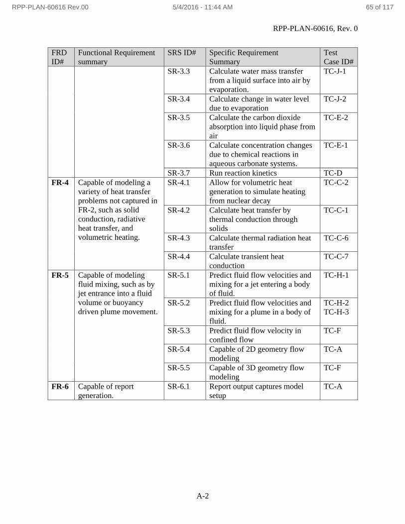
RPP-PLAN-60616, Rev. 0
A-2
FRD
ID#
Functional Requirement
summary
SRS ID# Specific Requirement
Summary
Test
Case ID#
SR-3.3 Calculate water mass transfer
from a liquid surface into air by
evaporation.
TC-J-1
SR-3.4 Calculate change in water level
due to evaporation
TC-J-2
SR-3.5 Calculate the carbon dioxide
absorption into liquid phase from
air
TC-E-2
SR-3.6 Calculate concentration changes
due to chemical reactions in
aqueous carbonate systems.
TC-E-1
SR-3.7 Run reaction kinetics TC-D
FR-4 Capable of modeling a
variety of heat transfer
problems not captured in
FR-2, such as solid
conduction, radiative
heat transfer, and
volumetric heating.
SR-4.1 Allow for volumetric heat
generation to simulate heating
from nuclear decay
TC-C-2
SR-4.2 Calculate heat transfer by
thermal conduction through
solids
TC-C-1
SR-4.3 Calculate thermal radiation heat
transfer
TC-C-6
SR-4.4 Calculate transient heat
conduction
TC-C-7
FR-5 Capable of modeling
fluid mixing, such as by
jet entrance into a fluid
volume or buoyancy
driven plume movement.
SR-5.1 Predict fluid flow velocities and
mixing for a jet entering a body
of fluid.
TC-H-1
SR-5.2 Predict fluid flow velocities and
mixing for a plume in a body of
fluid.
TC-H-2
TC-H-3
SR-5.3 Predict fluid flow velocity in
confined flow
TC-F
SR-5.4 Capable of 2D geometry flow
modeling
TC-A
SR-5.5 Capable of 3D geometry flow
modeling
TC-F
FR-6 Capable of report
generation.
SR-6.1 Report output captures model
setup
TC-A
RPP-PLAN-60616 Rev.00 5/4/2016 - 11:44 AM 65 of 117

RPP-PLAN-60616, Rev. 0
B-1
APPENDIX B
Test Case Execution Record
RPP-PLAN-60616 Rev.00 5/4/2016 - 11:44 AM 66 of 117

RPP-PLAN-60616, Rev. 0
B-2
Test Case Execution
Tester Name: Ryan M. Murray Date of Test: April, 2016
UCS Name: COMSOL Multiphysics, CFD Module, Heat
Transfer Module, Reaction Engineering Module UCS Version: 5.2.0.220
Test Hardware Configuration
Machine ID: WF33648 Model: Dell Precision Tower 7910
OS Software Windows 7 Enterprise ®, 64-bit Operating
System Excel Version: NA
Hardware: Intel® Xeon® CPU E5-2687W v3 @ 3.10GHz6
Processor, NVIDIA Quadro® K4200 graphics
card7, 128 GB RAM, 500GB primary HDD,
2TB secondary HDD.
Property
Number: WF33648
6 Intel and Xeon are registered trademarks of Intel Corporation, Santa Clara, CA 7 NVIDIA Quadro is a registered trademark of NVIDIA Corporation, Santa Clara, CA
RPP-PLAN-60616 Rev.00 5/4/2016 - 11:44 AM 67 of 117
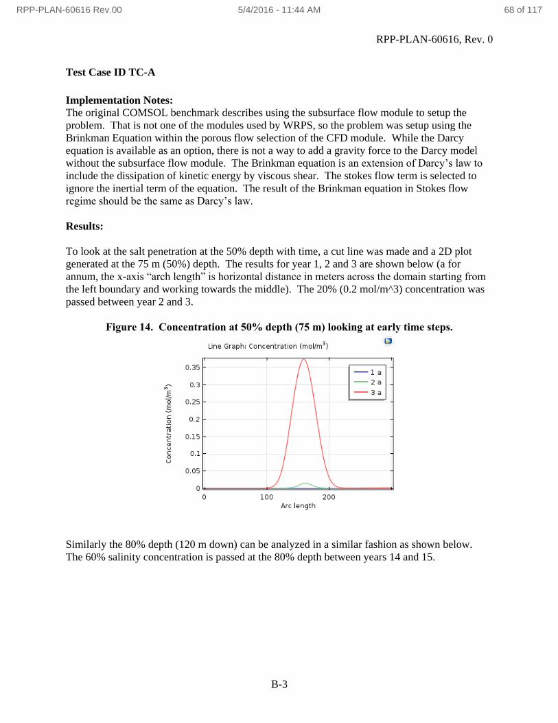
RPP-PLAN-60616, Rev. 0
B-3
Test Case ID TC-A
Implementation Notes:
The original COMSOL benchmark describes using the subsurface flow module to setup the
problem. That is not one of the modules used by WRPS, so the problem was setup using the
Brinkman Equation within the porous flow selection of the CFD module. While the Darcy
equation is available as an option, there is not a way to add a gravity force to the Darcy model
without the subsurface flow module. The Brinkman equation is an extension of Darcy’s law to
include the dissipation of kinetic energy by viscous shear. The stokes flow term is selected to
ignore the inertial term of the equation. The result of the Brinkman equation in Stokes flow
regime should be the same as Darcy’s law.
Results:
To look at the salt penetration at the 50% depth with time, a cut line was made and a 2D plot
generated at the 75 m (50%) depth. The results for year 1, 2 and 3 are shown below (a for
annum, the x-axis “arch length” is horizontal distance in meters across the domain starting from
the left boundary and working towards the middle). The 20% (0.2 mol/m^3) concentration was
passed between year 2 and 3.
Figure 14. Concentration at 50% depth (75 m) looking at early time steps.
Similarly the 80% depth (120 m down) can be analyzed in a similar fashion as shown below.
The 60% salinity concentration is passed at the 80% depth between years 14 and 15.
RPP-PLAN-60616 Rev.00 5/4/2016 - 11:44 AM 68 of 117

RPP-PLAN-60616, Rev. 0
B-4
Figure 15. Concentration at 80% depth (120 m) at later time steps.
Visually the results of the COMSOL study are very similar to other codes. Shown in Figure 16
are a number of time steps with the codes of comparison on the right and COMSOL on the left.
In the left side the COMSOL results show the 20% salt concentration in blue and the 60% in red.
On the right side the colors indicate the code used and both the 20 and 60% lines are the same
color, with the 20% line always lower than the 60%.
It is interesting how the general shape is very similar between the models but the fine detail
varies slightly. I consider the COMSOL results acceptably close to the results from the other
codes. Some differences can be noted. The slightly less intrusive penetration of the salt in the
COMSOL model on year 1 is likely due to the ramping gravity force and salt concentration in
year 1. It seems like this effect should be less significant by year 3, however we will see the
COMSOL results slightly behind the other codes. By year 10 their does not seem to be a
difference. Year 10 has a “finger” on the outer edge of the 20% concentration that does not
appear in the other codes until farther out in time. At year 20 COMSOL shows a “finger” still on
the edge of the 20% concentration, which matches the SUTRA code in general shape, however
the SUTRA code also predicts a finger on the 60% concentration which is not predicted by
COMSOL.
The original COMSOL application ID: 657 is different than the results generated in this test case
or in the reference data. Specifically the COMSOL application file does not have a high
centerline concentration at later times, while the literature codes and the results here do. The
main difference is likely the grid spacing, as the test case presented here uses almost 4 times as
many cells in the same area as the COMSOL application file. The result with more cells seems
RPP-PLAN-60616 Rev.00 5/4/2016 - 11:44 AM 69 of 117
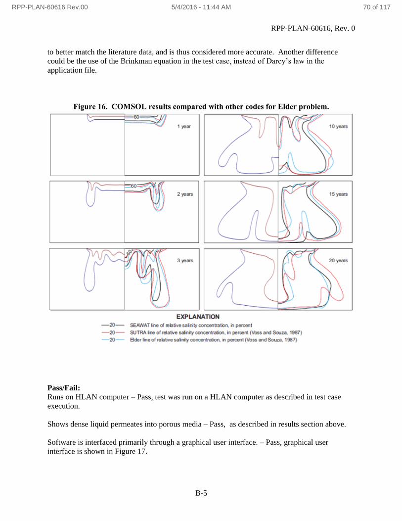
RPP-PLAN-60616, Rev. 0
B-5
to better match the literature data, and is thus considered more accurate. Another difference
could be the use of the Brinkman equation in the test case, instead of Darcy’s law in the
application file.
Figure 16. COMSOL results compared with other codes for Elder problem.
Pass/Fail:
Runs on HLAN computer – Pass, test was run on a HLAN computer as described in test case
execution.
Shows dense liquid permeates into porous media – Pass, as described in results section above.
Software is interfaced primarily through a graphical user interface. – Pass, graphical user
interface is shown in Figure 17.
RPP-PLAN-60616 Rev.00 5/4/2016 - 11:44 AM 70 of 117

RPP-PLAN-60616, Rev. 0
B-6
Figure 17. Graphical User Interface used to setup Constant-concentration (C=0.0)
boundary on bottom.
Report Output captures model setup – Pass. A variable “epsilon” was created and a set to a
value of 0.1. This is reported in the section 1.1 titled “Parameters” of the report output. Then in
section 2.3.1 under “Fluid and Matrix properties 1” the Porosity in the “Settings” table is set to
“User Defined” which is given a value of “epsilon”. The data is presented in Table 6.
Alternatively the value could have been entered directly without creating a variable, however by
creating variables for input values it makes it easier to review the model input.
RPP-PLAN-60616 Rev.00 5/4/2016 - 11:44 AM 71 of 117
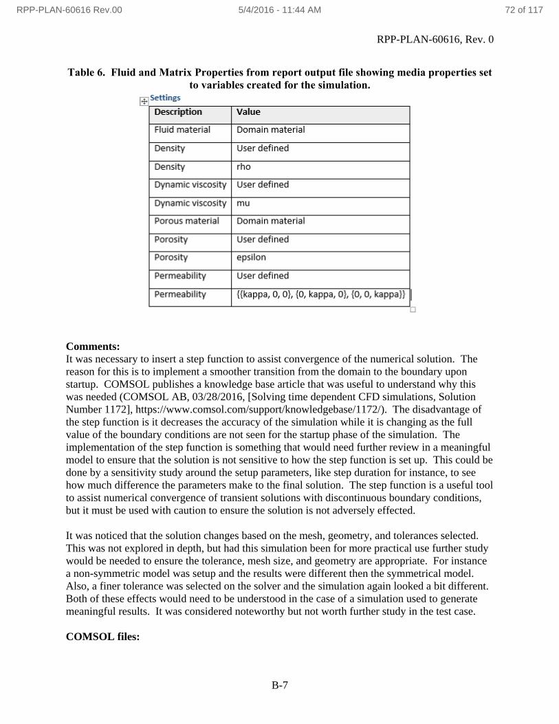
RPP-PLAN-60616, Rev. 0
B-7
Table 6. Fluid and Matrix Properties from report output file showing media properties set
to variables created for the simulation.
Comments:
It was necessary to insert a step function to assist convergence of the numerical solution. The
reason for this is to implement a smoother transition from the domain to the boundary upon
startup. COMSOL publishes a knowledge base article that was useful to understand why this
was needed (COMSOL AB, 03/28/2016, [Solving time dependent CFD simulations, Solution
Number 1172], https://www.comsol.com/support/knowledgebase/1172/). The disadvantage of
the step function is it decreases the accuracy of the simulation while it is changing as the full
value of the boundary conditions are not seen for the startup phase of the simulation. The
implementation of the step function is something that would need further review in a meaningful
model to ensure that the solution is not sensitive to how the step function is set up. This could be
done by a sensitivity study around the setup parameters, like step duration for instance, to see
how much difference the parameters make to the final solution. The step function is a useful tool
to assist numerical convergence of transient solutions with discontinuous boundary conditions,
but it must be used with caution to ensure the solution is not adversely effected.
It was noticed that the solution changes based on the mesh, geometry, and tolerances selected.
This was not explored in depth, but had this simulation been for more practical use further study
would be needed to ensure the tolerance, mesh size, and geometry are appropriate. For instance
a non-symmetric model was setup and the results were different then the symmetrical model.
Also, a finer tolerance was selected on the solver and the simulation again looked a bit different.
Both of these effects would need to be understood in the case of a simulation used to generate
meaningful results. It was considered noteworthy but not worth further study in the test case.
COMSOL files:
RPP-PLAN-60616 Rev.00 5/4/2016 - 11:44 AM 72 of 117

RPP-PLAN-60616, Rev. 0
B-8
TC-A.mph is the COMSOL run file, and is saved in the IDMS HISI Software Documentation
folder for COMSOL.
The report file is saved as a word document title TC-A in SmartPlant.
Test Case ID: TC-B
Implementation Notes:
Implementation was straightforward and following the COMSOL guide worked well.
Results:
The Nu number is defined as:
Where h is the local convective heat transfer coefficient, L is the surface length, and k is the
thermal conductivity. Based on the problem definition, L and k are both equal to 1. The heat
transfer coefficient is specified by:
h=q’/(T-Tf)
Where q’ is the heat flux per unit area and (T-Tf) is the temperature difference of the surface.
Again, based on the problem setup (T-Tf) is equal to 1. Thus the average Nu number becomes
equal to the average heat flux of the surface, which can be calculated with a line average within
COMSOL. The results are given in the following table.
Table 7. Average Nusselt Number Comparison Between Davis and COMSOL
Rayleigh
Number 103 104 105 106
Davis Nu
(Ave.)
1.118 2.243 4.519 8.800
COMSOL Nu
(Ave.)
1.118 2.246 4.525 8.831
The difference between the Davis paper and COMSOL are less than 1%. Other parameters could
be calculated, but the average Nusselt number was considered the most important and sufficient.
The plot comparison with published results from COMSOL is very similar. There is a slight
difference in how the contour lines are drawn (they show up darker in our simulation), but the
shape and values are very similar between the two. Contours are the x-axis component of the
velocity field, arrows are the velocity field magnitude and direction, and the surface plot is
temperature.
RPP-PLAN-60616 Rev.00 5/4/2016 - 11:44 AM 73 of 117

RPP-PLAN-60616, Rev. 0
B-9
Figure 18. Results for Natural Convection in a Square Cavity.
Pass/Fail:
Pass
Comments:
COMSOL Files:
TC-B.mph is the COMSOL run file, and is saved in IDMS HISI Software Documentation folder
for COMSOL
The report file is saved as a word document title TC-B in SmartPlant.
RPP-PLAN-60616 Rev.00 5/4/2016 - 11:44 AM 74 of 117

RPP-PLAN-60616, Rev. 0
B-10
Test Case ID: TC-C
Implementation Notes:
See case descriptions.
Results:
TC-C-1
The calculated heat transferred is 4249.999 W, which agrees well with the hand calculation value
of 4.25*10^3 W.
Figure 19. TC-C-1 Results
TC-C-2
A value of 1.125 W as calculated in COMSOL, this exactly matches the result of the hand
calculation of 1.125 W.
RPP-PLAN-60616 Rev.00 5/4/2016 - 11:44 AM 75 of 117

RPP-PLAN-60616, Rev. 0
B-11
Figure 20. TC-C-2 Results
TC-C-3
COMSOL simulation gave a value of 5724.49 W for the heat flux with a surface temperature of
1063.2653 K. The COMSOL result are the same as the hand calculation values for the surface
temperature and heat transfer rate.
RPP-PLAN-60616 Rev.00 5/4/2016 - 11:44 AM 76 of 117
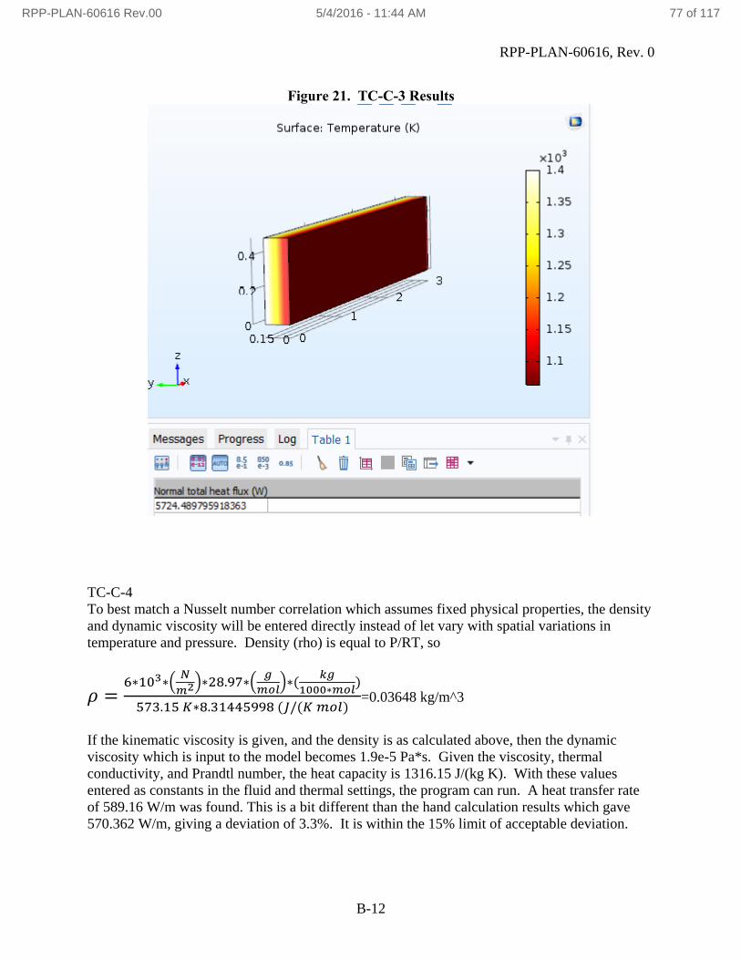
RPP-PLAN-60616, Rev. 0
B-12
Figure 21. TC-C-3 Results
TC-C-4
To best match a Nusselt number correlation which assumes fixed physical properties, the density
and dynamic viscosity will be entered directly instead of let vary with spatial variations in
temperature and pressure. Density (rho) is equal to P/RT, so
𝜌 =6∗103∗(
𝑁
𝑚2)∗28.97∗(𝑔
𝑚𝑜𝑙)∗(
𝑘𝑔
1000∗𝑚𝑜𝑙)
573.15 𝐾∗8.31445998 (𝐽/(𝐾 𝑚𝑜𝑙)=0.03648 kg/m^3
If the kinematic viscosity is given, and the density is as calculated above, then the dynamic
viscosity which is input to the model becomes 1.9e-5 Pa*s. Given the viscosity, thermal
conductivity, and Prandtl number, the heat capacity is 1316.15 J/(kg K). With these values
entered as constants in the fluid and thermal settings, the program can run. A heat transfer rate
of 589.16 W/m was found. This is a bit different than the hand calculation results which gave
570.362 W/m, giving a deviation of 3.3%. It is within the 15% limit of acceptable deviation.
RPP-PLAN-60616 Rev.00 5/4/2016 - 11:44 AM 77 of 117

RPP-PLAN-60616, Rev. 0
B-13
Two things to point out on this problem. First is that a much finer mesh was needed than the
other heat transfer problems to get an acceptable solution (mesh used had about 236k elements,
most meshes employed for test cases have less than half as many elements). Secondly, to get an
accurate value for the heat flux the model needed to include a shoulder region so that the plate
was away from the inlet or outlet boundary on each end, this way the integrated heat transfer
value did not include the boundary region on either end. This is very important to getting
accurate values.
Figure 22. TC-C-4 Results
TC-C-5
The COMSOL porous media conduction result is 157.28 W/m, which is the same as the value
calculated by hand.
RPP-PLAN-60616 Rev.00 5/4/2016 - 11:44 AM 78 of 117

RPP-PLAN-60616, Rev. 0
B-14
Figure 23. TC-C-5 Results
TC-C-6
The radiative heat flux per unit width calculated in COMSOL is -0.49686 W/m, which agrees
well with the value calculated by hand of -0.499 W/m. The slight difference is likely due to how
COMSOL discretizes space to create view factors for radiative heat transfer, compared with the
analytical solution used in the hand calculation.
RPP-PLAN-60616 Rev.00 5/4/2016 - 11:44 AM 79 of 117

RPP-PLAN-60616, Rev. 0
B-15
Figure 24. TC-C-6 Results
TC-C-7
Drawing a contour line at 0 C on day 60 gives a depth of 0.666 m. This is an error of 2%
compared with the hand calculation of 0.677m. The plot of temperature and depth for different
times is as expected. Arc length is the distance in meters from the surface.
RPP-PLAN-60616 Rev.00 5/4/2016 - 11:44 AM 80 of 117

RPP-PLAN-60616, Rev. 0
B-16
Figure 25. TC-C-7 Results
Pass/Fail:
Pass
Comments:
The convective heat transfer problem, TC-C-4 showed the most variation. The Nusselt number
correlations are empirically based and probably not good to better than 15% accuracy.
COMSOL offers capabilities, such as spatially calculating physical properties based on
temperature and other parameters, that should be able to improve on the accuracy of the Nusselt
number correlations. Within COMSOL there are also different ways of treating the boundary
layer, and these should be explored if a more accurate convective calculation is desired.
A step function was necessary to create a smooth transition for the temperature boundary in TC-
C-7. It could be implemented either as a spatial step in the initial temperature field or temporally
in the boundary condition. COMSOL has information on smoothing in their knowledge base
articles (COMSOL AB, 03/28/2016, [Smoothed step transitions in COMSOL Multiphysics,
Solution Number 905], http://www.comsol.com/support/knowledgebase/905/).
One thing to note in COMSOL which was discovered when working on the convection problem
is the difference between reference pressure (pref), pressure (p), and absolute pressure (pA). The
absolute pressure is the reference pressure plus the pressure. The reference pressure is specified
as the baseline pressure in the model on the settings page of the flow module. The pressure (p) is
RPP-PLAN-60616 Rev.00 5/4/2016 - 11:44 AM 81 of 117

RPP-PLAN-60616, Rev. 0
B-17
like a gauge pressure. When specifying a pressure below atmospheric, the reference pressure
needs to be adjusted to give the correct value of total pressure.
COMSOL Report:
The model files are available in IDMS HISI Software Documentation folder for COMSOL as
TC-C-1.mph, TC-C-2.mph, TC-C-3.mph, TC-C-4.mph, TC-C-5.mph, TC-C-6.mph, and TC-C-
7.mph.
The report files are is saved as a word document with the same case prefix in SmartPlant.
RPP-PLAN-60616 Rev.00 5/4/2016 - 11:44 AM 82 of 117

RPP-PLAN-60616, Rev. 0
B-18
Test Case ID: TC-D
Implementation Notes:
This problem provides a good example of how to use the reaction chemistry module within a
flow problem. Note that the reactions are setup within the Chemistry module, and then a
“Reaction” field is added to the species transport to implement the reactions spatially.
The multiphysics coupling is used in this test case. When physics are coupled through this
interface, some parameters cannot be specified directly within the module. For instance in
laminar flow, fluid properties, the density is grayed out (not selectable) because the multiphysics
flow coupling is used and the density calculation is done within the chemistry module.
Results:
Results are very similar to the expected values. The maximum conversion at the outlet is 0.8385,
which is within 0.025 of the expected value of 0.85. The half axial location gives conversion
between 0.165 and 0.4648, which are between the expected limits of 0.15 and 0.5.
Figure 26. Radial temperature profile for TC-D
RPP-PLAN-60616 Rev.00 5/4/2016 - 11:44 AM 83 of 117
RPP-PLAN-60616, Rev. 0
B-19
Pass/Fail:
Pass
Comments:
It should be noted that figure E8-12.2 in Fogler is not clear about the conditions used to generate
the figure, as a number of different cases were run (adiabatic, non-adiabatic, plug flow, and
laminar flow). Additionally the concentration and physical properties are a bit unclear (for
example, Figure E-8-12.1 states a concentration for cA0 of 2454, presumably mol/m^3, whereas
the problem statement gives propylene oxide as 1 part in 4.5 parts by volume which given a
density of 830 kg/m^3, molecular weight of 58.095 g/mole, that would be 3175 mol/m^3. The
COMSOL case description uses 1587.4 mol/m^3). The figure in the Fogler text compares better
with the plug flow setup (COMSOL AB, 03/28/2016, [Tubular Reactor With Nonisothermal
Cooling Jacket, Application ID 67], http://www.comsol.com/model/tubular-reactor-with-
nonisothermal-cooling-jacket-67), but still does not match exactly (likely due to other setup
parameters being different). An analytical solution is provided for the isothermal plug flow case,
but that is less useful for us as it does not provide a coupled test case showing reactions, heat,
and mass transport.
COMSOL Report:
The model file is saved as TC-D.mph within IDMS HISI Software Documentation folder for
COMSOL, and the word document report file is saved in SmartPlant.
RPP-PLAN-60616 Rev.00 5/4/2016 - 11:44 AM 84 of 117
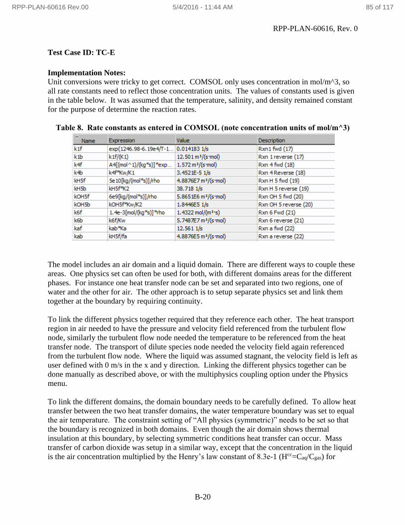
RPP-PLAN-60616, Rev. 0
B-20
Test Case ID: TC-E
Implementation Notes:
Unit conversions were tricky to get correct. COMSOL only uses concentration in mol/m^3, so
all rate constants need to reflect those concentration units. The values of constants used is given
in the table below. It was assumed that the temperature, salinity, and density remained constant
for the purpose of determine the reaction rates.
Table 8. Rate constants as entered in COMSOL (note concentration units of mol/m^3)
The model includes an air domain and a liquid domain. There are different ways to couple these
areas. One physics set can often be used for both, with different domains areas for the different
phases. For instance one heat transfer node can be set and separated into two regions, one of
water and the other for air. The other approach is to setup separate physics set and link them
together at the boundary by requiring continuity.
To link the different physics together required that they reference each other. The heat transport
region in air needed to have the pressure and velocity field referenced from the turbulent flow
node, similarly the turbulent flow node needed the temperature to be referenced from the heat
transfer node. The transport of dilute species node needed the velocity field again referenced
from the turbulent flow node. Where the liquid was assumed stagnant, the velocity field is left as
user defined with 0 m/s in the x and y direction. Linking the different physics together can be
done manually as described above, or with the multiphysics coupling option under the Physics
menu.
To link the different domains, the domain boundary needs to be carefully defined. To allow heat
transfer between the two heat transfer domains, the water temperature boundary was set to equal
the air temperature. The constraint setting of “All physics (symmetric)” needs to be set so that
the boundary is recognized in both domains. Even though the air domain shows thermal
insulation at this boundary, by selecting symmetric conditions heat transfer can occur. Mass
transfer of carbon dioxide was setup in a similar way, except that the concentration in the liquid
is the air concentration multiplied by the Henry’s law constant of 8.3e-1 (Hcc=Caq/Cgas) for
RPP-PLAN-60616 Rev.00 5/4/2016 - 11:44 AM 85 of 117

RPP-PLAN-60616, Rev. 0
B-21
carbon dioxide (Wikipedia, 03/28/2016, [Henry’s Law],
https://en.wikipedia.org/wiki/Henry%27s_law).
In TC-E-2 the run time was slow. This was improved by running the laminar flow field once and
using the velocity generated without updating the flow solution. This should be a good
approximation because the flow is not expected to change. Also, reaction 1 and 5OH- were
changed to irreversible forward reactions (as the backwards reaction was relatively slow due to
either the rate constant value or the concentrations used), and equation 6 and “a” were changed
to equilibrium reactions. This allowed the kinetics to calculate much faster.
Results:
TC-E-1:
CO2 was found to be 0.0856 mol/m^3 (or mmol/kg if density of 1000 kg/m^3 is assumed) at 100
seconds, this is within the criteria of between 0.05 and 0.15 mol/m^3. The shape of the curve
matches closely the value in the paper. Two selected plots are shown below. The curves are not
exactly the same as the reference, but they are acceptably close for the simplifying assumptions
made. Note, to simplify notation the charges are not included in the species identifiers below
(the program internal variable names were used, this could be changed but it takes more time to
generate the plot), it is know they are charged ions.
Figure 27. Species reaction over time for TC-E-1, scaled for carbon dioxide.
RPP-PLAN-60616 Rev.00 5/4/2016 - 11:44 AM 86 of 117

RPP-PLAN-60616, Rev. 0
B-22
Figure 28. Species reaction over time for TC-E-1, scaled for carbonate ion.
TC-E-2:
The physical property hand calculation almost exactly matches the value in COMSOL. The
table below shows the value of the concentration, temperature, and density, taken from the model
at the given time and coordinates listed. The percent difference between the density found in
COMSOL and the density calculated by hand is very small, and well within the acceptance
criteria.
Table 9. Physical Property Calculation Results
Time
(Day)
x y Concentration
(mol/m^3)
Temperature
(K)
COMSOL
Density
(kg/m^3)
Density
Calculation
(kg/m^3)
%
Difference
1 0.05 0.05 798 301 1155 1155 -1.9E-03
1 0.05 0.45 799 319 1145 1145 1.6E-03
1 0.95 0.05 15199 301 1564 1564 -7.3E-04
1 0.95 0.45 15199 329 1548 1548 2.9E-03
The inter-conversion reaction of carbon dioxide, bicarbonate, and carbonate is fast relative to the
mass transfer of carbon dioxide. Therefore carbonate buildup as the terminal reaction production
RPP-PLAN-60616 Rev.00 5/4/2016 - 11:44 AM 87 of 117

RPP-PLAN-60616, Rev. 0
B-23
in high pH environments is the best marker for reaction progress. The figure below shows the
carbonate concentration at the end of one year for the reaction described. The carbonate
concentration has increased by more than 1000 mol/m^3 at the end of one year in the region of
greatest concentration.
Figure 29. Carbonate concentration after one year for test case problem.
The carbonate buildup at first seems strange it’s not on the left hand side as that is the inlet side
in the model, however given the hydroxide gradient and only diffusion transport it makes sense.
The hydroxide concentration after one year is shown below. In areas with high hydroxide,
carbon dioxide can’t build up on the surface as it reacts away. In areas of low hydroxide
concentration, the carbon dioxide build up on the surface as it is diffusion limited to transport
away, and this reduced the carbon dioxide transfer in that region. In the region of highest
carbonate concentration the hydroxide concentration has been reduced.
RPP-PLAN-60616 Rev.00 5/4/2016 - 11:44 AM 88 of 117
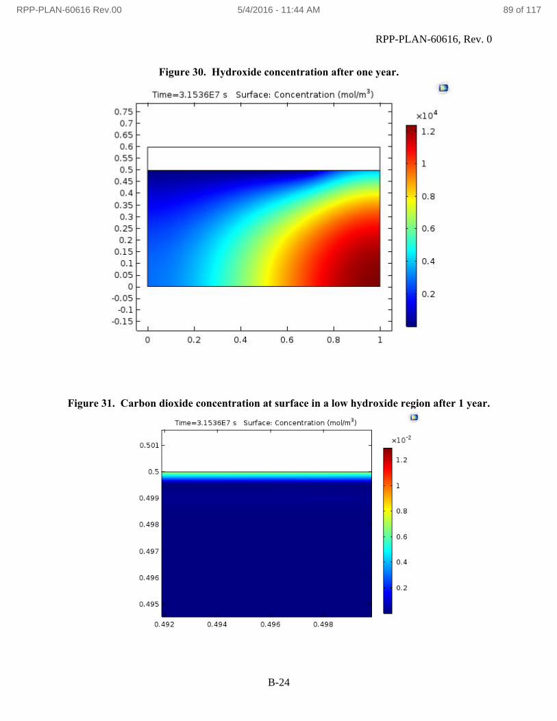
RPP-PLAN-60616, Rev. 0
B-24
Figure 30. Hydroxide concentration after one year.
Figure 31. Carbon dioxide concentration at surface in a low hydroxide region after 1 year.
RPP-PLAN-60616 Rev.00 5/4/2016 - 11:44 AM 89 of 117

RPP-PLAN-60616, Rev. 0
B-25
As a test, a model was run with high and uniform hydroxide concentration. In that case the
carbonate builds up on the left side as expected. The strange concentration distributions seen in
the test case are an artifact of eliminating the convective currents in the liquid phase and the
hydroxide gradient setup as an initial conditions to test the concentration and temperature
dependent density equation.
Figure 32. Carbonate concentration after 1 year with high and uniform hydroxide in the
liquid phase.
Pass/Fail:
TC-E-1: Pass
Expected CO2 concentration at 100 seconds is within passing criteria.
TC-E-2: Pass
Physical properties calculated by hand match the COMSOL results almost exactly.
Evidence of carbon dioxide diffusion into the liquid and reaction is evident by the carbonate
buildup over time.
RPP-PLAN-60616 Rev.00 5/4/2016 - 11:44 AM 90 of 117

RPP-PLAN-60616, Rev. 0
B-26
Comments:
When dealing with concentration in COMSOL, it’s important to note that concentration is
always in mol/m^3. In some instances different units sets can be specified and the program will
convert, however it seemed least likely to cause an error to enter the molar concentration
directly.
When editing reaction rate equations, for instance in a case where the concentration of water is
ignored as a solvent, the expected rate constant and the implemented rate constant will not have
the same units (if the program is expecting dC/dt=k*[A]*[B], and you edit the reaction to be
dC/dT=k*[A], the units of k will be 1/sec, not L/(mol*sec) as it would be with the former rate).
This causes an “inconstant units” flag in the program (yellow coloring to the text). This can be
ignored, and the program will run as if the correct units are in place.
When reactions occur with very small concentrations the solver can sometimes have issues as it
can create the potential for a division by zero error when running the solver mathematics. This
can be avoided by putting an arbitrarily small value in place of zero. For instance a value of 1e-8
mol/m^3 was used for species that could be reacted to form in the system, and 1e-12 mol/m^3
for species that will not be present in the system was used in this model. Another observation is
that negative species concentrations can occur due to the problem setup. This can be avoided in
a few different ways (COMSOL has an article on the topic that is useful COMSOL AB,
03/28/16, [Avoiding negative concentrations, Solution Number 952],
https://www.comsol.com/support/knowledgebase/952/). One is to refine the mesh, or at least
make sure the mesh is sufficiently resolved for the problem setup. Checking the wall lift off or
wall resolution is one way to check the mesh. Another suggestion is to place a “lower limit” on
the value by right clicking the “Segregated” solver and adding it to the solution. A lower limit
can be entered (for instance “comp3.c2HCO3 1E-10”) to keep the solver from using negative
values.
Reactions can be input in a number of different ways. One observation is that entering a reaction
as reversible with a forward and reverse rate constant seemed more stable than using equilibrium
reactions. It is possible this is because equilibrium reactions need to have initial values that are
near equilibrium.
Stability of a run was often an issue with this problem. There are multiple physics and domains
that are coupled, and that makes it a fairly complicated model. One way to achieve a solution
was to run the model for short time periods, then setup a subsequent solver where the previous
solver left off. In some cases it can be advantageous to turn physics on or off for different solver
intervals to simplify the calculations, however running a fully coupled solution for this problem
did not seem to take noticeably longer and seemed more stable. When running off of previous
results, especially if not all physics are being run, it is important to set both “initial values of
variables solved for” and “values of variables not solved for” to the last time step of the previous
solution. Another note is that the adaptive time step cannot change too drastically. Sometimes it
can be advantageous to manually enter a very small time step and let it increase as needed, rather
than starting with too large of a time step and having the solver fail before it could be reduced to
a value that would allow the simulation to run.
RPP-PLAN-60616 Rev.00 5/4/2016 - 11:44 AM 91 of 117

RPP-PLAN-60616, Rev. 0
B-27
The flux of CO2 entering the liquid should equal the flux leaving the gas phase. When the
surface integral of the boundary CO2 flux is taken on each domain the values are close but not a
match. For the end of one year, the integrated domain fluxes for carbon dioxide are -1.8619E-5
mol/(m*s) for the liquid domain vs. 1.6355e-5 mol/(m*s) for the gas domain. These are plotted
below. COMSOL technical support recommended using a pointwise constraint to achieve
consistent flux values, but this was not successful to implement for transient solutions (it did
work for steady state however). Another option would be to enter an equation for the mass
transfer across the interface as a flux input to each boundary region, this would ensure the same
value is used for both sides, but it requires knowing a mass transfer coefficient to use. The
discrepancy in boundary flux observed will represent a mass balance error, and further work
would need to be done to ensure these values match for more accurate analysis.
Figure 33. Boundary flux of carbon dioxide entering the liquid (blue) and leaving the gas
phase (green), along the length of the surface.
Initially the discrepancy was greater, but by changing the integration line to exclude the end
point which share a boundary with the inlet and outlet the values were in better agreement.
RPP-PLAN-60616 Rev.00 5/4/2016 - 11:44 AM 92 of 117

RPP-PLAN-60616, Rev. 0
B-28
Figure 34. Illustration showing how the very edge of the surface was excluded so that the
inlet and outlet gas flow boundaries would not be captured in the flux calculation for the
liquid surface.
The solver needed to be optimized to allow this problem to run. The solver type needed to be
changed from “Fully Coupled” to “Segregated”, and the “Direct” solver used instead of the
“Direct 1” solver. Also an additional “Lower Limit 1” needed to be added to the Segregated
solver with a lower bound for species concentrations. Each species is entered as
“comp3.cCO2Air 1E-10” to place a lower limit on the concentration to avoid a negative value.
Lastly mesh size was important for this problem as a “normal” mesh was too course to run well
and caused solver errors.
COMSOL Report:
The model files are available in IDMS HISI Software Documentation folder for COMSOL as
TC-E-1.mph, and TC-E-2.mph.
The report files are is saved as word documents with the same case prefix in SmartPlant.
RPP-PLAN-60616 Rev.00 5/4/2016 - 11:44 AM 93 of 117

RPP-PLAN-60616, Rev. 0
B-29
Test Case ID: TC-F
Implementation Notes:
The original problem used a 10 ft length and a 0.1 psi pressure drop. To simplify the problem a
1 ft length with 0.01 psi pressure drop was used. The equation for velocity has the pressure drop
(P0-PL) divided by Length (L), so as long as the pressure gradient remains the same the results
hold.
Results:
TC-F-1:
With a pressure boundary condition, the velocity profile is essentially unchanged through the
length of the pipe. The plot below as made 0.25m from the inlet, and the maximum velocity
found is 0.2987 ft/s. This agrees well with 0.299 ft/sec. Note arc length is displaying in meters
and corresponds to a line across the diameter of the pipe.
When the output is given in m/s a value of 0.0911 m/s was found. The imperial unit answer
converts to a value of 0.0910 m/s (0.2987 (ft/s)*(1m/3.28084ft)=0.0910 m/s). The difference is
within the passing criteria. The answer is most likely not exactly the same due to uncertainty in
reading the value from the plot generated.
Figure 35. Velocity profile in pipe
The model run was in 3D. The geometry is shown in the figure below.
RPP-PLAN-60616 Rev.00 5/4/2016 - 11:44 AM 94 of 117

RPP-PLAN-60616, Rev. 0
B-30
Figure 36. 3D geometry used in confined flow problem.
As a side note, the turbulent flow model k-ε was used and a result of 0.2987 ft/sec was obtained
with a very similar profile. This indicates that the turbulence model can at times simulate
laminar flow, albeit at a higher computational cost.
TC-F-2:
The figure below shows the development of a flow profile when a constant velocity inlet is used.
Distance is in meters from the inlet. The second distance, 0.0006096, is interesting in that it does
not have a maximum at the centerline. This does not match up with the classical view of a
developing flow profile. The variation accounts for less than 10% of the velocity profile in the
leading edge.
RPP-PLAN-60616 Rev.00 5/4/2016 - 11:44 AM 95 of 117

RPP-PLAN-60616, Rev. 0
B-31
Figure 37. Velocity profile development.
The velocity profile is not unlike what has been reported in literature for low Re number flow.
Shown below is a plot from Santos paper (Santos, R.G., Figueiredo, J.R., Laminar elliptic flow
in the entrance region of tubes, J. Braz. Soc. Mech. Sci. & Eng. vol.29 no.3 Rio de
Janeiro July/Sept. 2007, Accessed on 2/10/2016, http://dx.doi.org/10.1590/S1678-
58782007000300001), showing half of the velocity profile for flow in a pipe. The center of the
pipe is at the left side and the wall at the right. Note the centerline velocity being a local
minimum rather than the maximum which occurs closer to the edge. This provides some
indication that the flow profile generated by COMSOL, while somewhat unexpected, are within
the range of expected results based on published data.
RPP-PLAN-60616 Rev.00 5/4/2016 - 11:44 AM 96 of 117

RPP-PLAN-60616, Rev. 0
B-32
Figure 38. Example of low Re number flow velocity profile in the entrance region, from
Santos.
Pass/Fail:
Pass
Comments:
A tip for working with COMSOL is that when switching between flow models (laminar or
turbulent and the different turbulent models) is that they can be selected within the existing flow
model on the main settings page under “Physical Model”. This way all of the boundary
conditions and setup information remain unchanged and one does not need to reestablish links
with other modules. The solver however can be turbulent model specific, so sometimes when
switching the turbulent model a new solution setup needs to be added so that the defaults for the
selected turbulent model are included.
COMSOL Report:
The model files are available in IDMS HISI Software Documentation folder for COMSOL as
TC-F-1.mph and TC-F-2.mph.
The report file is saved as word documents with the same case prefix in SmartPlant.
RPP-PLAN-60616 Rev.00 5/4/2016 - 11:44 AM 97 of 117
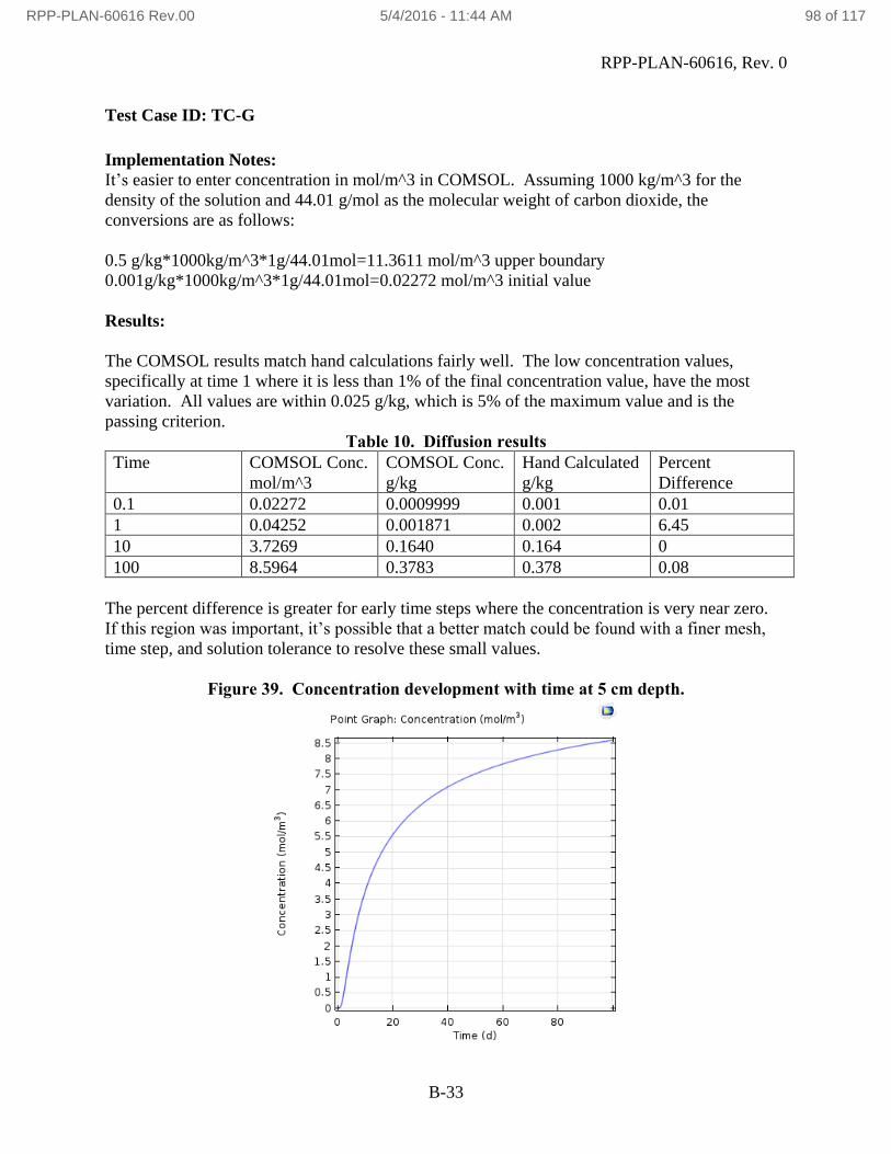
RPP-PLAN-60616, Rev. 0
B-33
Test Case ID: TC-G
Implementation Notes:
It’s easier to enter concentration in mol/m^3 in COMSOL. Assuming 1000 kg/m^3 for the
density of the solution and 44.01 g/mol as the molecular weight of carbon dioxide, the
conversions are as follows:
0.5 g/kg*1000kg/m^3*1g/44.01mol=11.3611 mol/m^3 upper boundary
0.001g/kg*1000kg/m^3*1g/44.01mol=0.02272 mol/m^3 initial value
Results:
The COMSOL results match hand calculations fairly well. The low concentration values,
specifically at time 1 where it is less than 1% of the final concentration value, have the most
variation. All values are within 0.025 g/kg, which is 5% of the maximum value and is the
passing criterion.
Table 10. Diffusion results
Time COMSOL Conc.
mol/m^3
COMSOL Conc.
g/kg
Hand Calculated
g/kg
Percent
Difference
0.1 0.02272 0.0009999 0.001 0.01
1 0.04252 0.001871 0.002 6.45
10 3.7269 0.1640 0.164 0
100 8.5964 0.3783 0.378 0.08
The percent difference is greater for early time steps where the concentration is very near zero.
If this region was important, it’s possible that a better match could be found with a finer mesh,
time step, and solution tolerance to resolve these small values.
Figure 39. Concentration development with time at 5 cm depth.
RPP-PLAN-60616 Rev.00 5/4/2016 - 11:44 AM 98 of 117
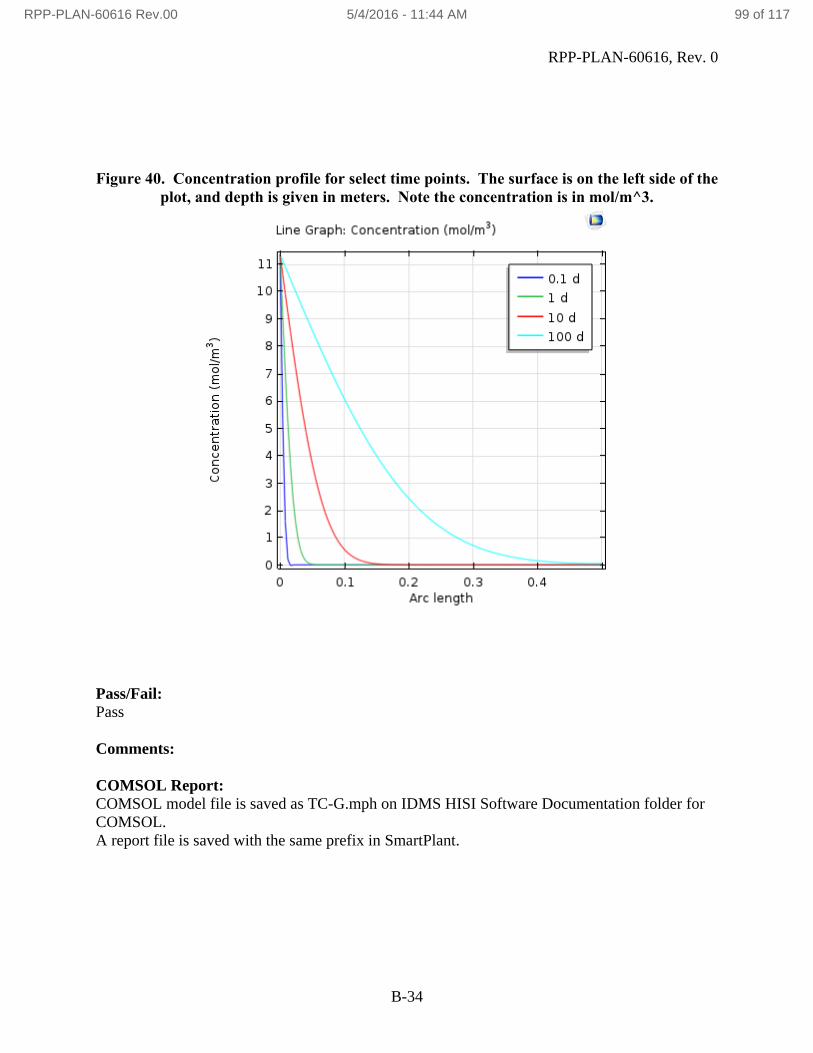
RPP-PLAN-60616, Rev. 0
B-34
Figure 40. Concentration profile for select time points. The surface is on the left side of the
plot, and depth is given in meters. Note the concentration is in mol/m^3.
Pass/Fail:
Pass
Comments:
COMSOL Report:
COMSOL model file is saved as TC-G.mph on IDMS HISI Software Documentation folder for
COMSOL.
A report file is saved with the same prefix in SmartPlant.
RPP-PLAN-60616 Rev.00 5/4/2016 - 11:44 AM 99 of 117

RPP-PLAN-60616, Rev. 0
B-35
Test Case ID: TC-H
Implementation Notes:
Finding converged solutions was difficult. Often a singularity error would occur, most likely due
to too coarse a mesh spacing. The corner of the inlet nozzle was one location of concern
specifically as the velocity has a potential singularity their due to the problem geometry. An
inlet nozzle helped the solution, probably because it allowed for some edge effects to develop
before hitting the corner. A fillet section on the corner (rounded corner) helped avoid the
singularity but was not used. A solution was found by first running the simulation as a transient
problem with a step function on the velocity and concentration, then running the steady state
solution based on a partly converged transient simulation.
It was possible to enter the hand calculations for expected velocity into the COMSOL program
(not as part of the flow calculations, but as independent variables riding on the solution spatial
field) so that a comparison could be made of these predicted values and the values in COMSOL.
These plots were made using a cut line, an example is plotted in the figure below.
Figure 41. 2D Cut line location for plots in TC-H-1
RPP-PLAN-60616 Rev.00 5/4/2016 - 11:44 AM 100 of 117

RPP-PLAN-60616, Rev. 0
B-36
Results:
TC-H-1:
Two sources can be checked for hand calculations, Blevins and Wiegel. The plot below shows
the velocity of a cut line from the centerline at a distance 4m from the outlet nozzle out radially.
Figure 42. Velocity calculated with COMSOL (solid blue), Wiegel (red dash), and Blevins
(Green dash).
The value found in COMSOL of the centerline velocity at 4m of 0.937 m/s compares well with
the value from Blevins of 0.9 m/s (4.1% difference).
RPP-PLAN-60616 Rev.00 5/4/2016 - 11:44 AM 101 of 117

RPP-PLAN-60616, Rev. 0
B-37
Figure 43. Revolved velocity plot from 2D axi-symmetric model for neutral turbulent jet.
Similarly concentration at the centerline of the jet 4 m distance from the nozzle is 0.5 mol/m^3
with the Blevins correlation and 0.5214 with COMSOL (4.3% difference).
Figure 44. Concentration calculated with COMSOL (solid blue), Wiegel (red dash), and
Blevins (Green dash).
RPP-PLAN-60616 Rev.00 5/4/2016 - 11:44 AM 102 of 117

RPP-PLAN-60616, Rev. 0
B-38
TC-H-2:
Velocity calculated with COMSOL at the centerline at a distance of 4m is 0.688 m/s, which
compares to 0.575 m/s from Blevins (19.7% difference). Wigel provides two correlations for
plume dispersion, one referenced to Abraham and the other to Morton, they are shown in the
plots below. While the agreement with Blevins is not as good as the previous subcase, the
COMSOL result is within the range of correlations for plume flow.
Figure 45. Velocity (m/s) calculated with COMSOL (solid blue), Wiegel per Abraham
method (red dash), Wiegel per Morton (orange dash), and Blevins (green dash), for an
axial cut from the centerline out radially at 4 m from the nozzle.
Concentration calculated with COMSOL at the 4 m out centerline position is 0.0428 g/mol,
which compares with a value of 0.038 g/mol from Blevins (12.6% difference).
RPP-PLAN-60616 Rev.00 5/4/2016 - 11:44 AM 103 of 117

RPP-PLAN-60616, Rev. 0
B-39
Figure 46. Concentration calculated with COMSOL (solid blue), Wiegel per Abraham
method (red dash), Wiegel per Morton (orange dash), and Blevins (Green dash).
Figure 47. Velocity for 2D axi-symmetric model for dense turbulent plume.
RPP-PLAN-60616 Rev.00 5/4/2016 - 11:44 AM 104 of 117

RPP-PLAN-60616, Rev. 0
B-40
TC-H-3:
The equation provided in Blevins for jet penetration when the buoyancy force is opposing the
momentum gives a value of 1.112 m for the maximum jet depth. COMSOL shows 0.655 m
(assuming 10% concentration of the incoming fluid as the point of maximum jet penetration).
This is a difference of 41%. The correlation in Blevins uses an empirical constant, alpha, which
has a value that is reported to range from 1.5 to 2.1, with 1.95 being representative (and the value
used). A plot is shown below. Note that arbitrary concentration units were used from 0 to 1 to
scale the density of the solution with. The large range of the empirical constant however
indicates the correlation has more variability to it than some of the other values that can be
calculated. It is good to note however that COMSOL may show jet penetration depths that are
on the low side of the possible range of values.
Figure 48. Concentration distribution of penetrating jet.
There are different ways to calculate the depth of a penetrating jet that are presented in literature.
Using the methodology of RPP-39013, section 2.3.1, a depth of 0.664 m can be calculated for the
jet penetration, and this agrees very well with the result form COMSOL. The document EPA-
660/2-73-012, Anderson et. al., Negatively Buoyant Jets In A Cross Flow, US EPA, October
1973 provides four correlations for penetration depth, and they all give values around 1 m.
Pass/Fail:
TC-H-1: Pass
Difference between hand calculations and velocity were 4.1%, and concentration were 4.%,
which is below the passing criteria of 10%.
TC-H-2: Pass
RPP-PLAN-60616 Rev.00 5/4/2016 - 11:44 AM 105 of 117

RPP-PLAN-60616, Rev. 0
B-41
Difference between hand calculations and velocity were 19.7%, and concentration were 12.6%,
which are both below the passing criteria of 20%.
TC-H-3: Pass
Difference between hand calculations for penetration depth and COMSOL result were 41%,
which is below the passing criteria of 50%.
Comments:
The SST turbulence model was chosen because it gave the best agreement with hand
calculations. Also, some references note SST is better able to handle turbulent jets (For instance
Wilkening, Heinz, Baraldi, Daniele, & Heitsch, Matthias (2007). On the importance of validation
when using commercial CFD codes in nuclear reactor safety. Nuclear Energy Agency of the
OECD (NEA): Organization for Economic Co-Operation and Development - Nuclear Energy
Agency.). For comparison, the k-omega turbulence model gave quite different results, as shown
below in the plot for velocity which should match the plot in TC-H-1. The COMSOL technical
article suggest using k-omega for jet flow (COMSOL Blog, 03/28/2016, [Frei, W., Which
Turbulence Model Should I Choose for My CFD Application?, 09/16/13],
http://www.comsol.com/blogs/which-turbulence-model-should-choose-cfd-application/),
however based on the poor correlation seen it does not work in all jet flow cases.
Figure 49. Velocity profile in m/s at 4m from outlet shown from centerline out radially for
k-omega turbulence model.
The solution space of various turbulence models was not explored in detail. One note to make is
the mesh refinement necessary for a converged solution changes with the different turbulence
models selected. Initially sensitivity studies were done showing little variation, however on a
finer mesh difference between the different turbulence models became apparent.
RPP-PLAN-60616 Rev.00 5/4/2016 - 11:44 AM 106 of 117

RPP-PLAN-60616, Rev. 0
B-42
It is likely that better agreement could be found by optimizing the turbulence model parameters.
The table below shows, as an example, the default SST model turbulence parameters. These are
easily adjustable within COMSOL, however their manipulation requires further study to do so
correctly. Some studies (See table 13 in Tschaepe, Lee Paul, "Liquid Jet Experiments and
Simulations for a Verification and Validation Study. " PhD diss., University of Tennessee, 2012.
http://trace.tennessee.edu/utk_graddiss/1360) alter the turbulence parameters to optimize their
solution.
Table 11. Default SST Turbulence Model Parameters
Other jet mixing type problems were considered. One problem specifically was looking at a
horizontal helium jet emitted from an orifice based on 4.3 of Xiao (Science and Technology of
Nuclear Installations, Volume 2009, 03/28/2016, [Xiao, J., Travis, J.R., Breitung, W., “Non-
Boussinesq Integral Model for Horizontal Turbulent Buoyant Round Jets,”, 2009],
http://www.hindawi.com/journals/stni/2009/862934/). This problem turned out to be difficult to
implement. Singularity errors were common, and could be resolved by running on finer mesh
size, however this incurred a computation cost that was difficult to get around as the models with
mesh fine enough to run would take days to compute. The Euler-Euler multiphase
implementation was the most stable to run, however an open boundary option is not available, so
the problem was again difficult to create a domain large enough to avoid edge effects but small
enough to run in a short time period. A dilute phase model with an equation for density based on
the species concentration was also tried. This method was not very stable and solutions often
crashed after a second or two simulation time. The problem also calls for an orifice, which
without a good axi-symmetric geometry is difficult to implement in 2D. A 3D model was tested,
but again the run time was too long to get a solution easily within a day. It is likely that a
suitable solution could be obtained with COMSOL, however it was decided that the effort was
not worth the time for the software management plan. If studies involving helium jets in air (or
generically compressible jets of widely varying density) are needed the problem can be revised.
Concentration in COMSOL is in mol/m^3. In this problem g/mol^3 is the concentration unit of
interest. Using the transport of dilute species interface the concentration is a bit arbitrary for the
fictional concentration employed. A conversion of 1 mol/g was assumed so that mol/m^3 and
g/mol^3 could be used interchangeably. Since no reactions or conversion are done within the
RPP-PLAN-60616 Rev.00 5/4/2016 - 11:44 AM 107 of 117

RPP-PLAN-60616, Rev. 0
B-43
program and equations for how species dependent physical properties are setup are well defined
this method can be employed.
One tip for getting to a converged solution is to first solve a transient solution with a ramping
boundary layer (COMSOL AB, 03/28/2016, [Solving time dependent CFD simulations, Solution
Number 1172], https://www.comsol.com/support/knowledgebase/1172/). The ramping boundary
layer is implemented by adding a step function (Under “Definitions” and “More Functions”
menu). The step function is setup such that it provides a ramping from 0 to 1 over a brief period
of initial time (this depends on the model, usually a second, but for longer runs like in the Elder
problem which runs for 20 years it could be a 1 year period of time). The step function is set as a
function of time (i.e. step1(t[1/s])). It is needed so that there is not a discontinuity between the
boundary condition and the solution field. Once a transient solution has been obtained at a
sufficient time that it nears the steady state solution, a steady state solution can be run with the
results of the transient analysis as the initial conditions (in the solver under “Values of
Dependent Variables” set the “Initial values of variables solved for” to the last time step solution
of the transient run, if not all variables are solved for such as when omitting one of the modules,
the “Values of variables not solved for” needs to be set as well).
One tip found when running this problem for avoiding a segregated step error is to use the
“Direct” solver instead of the “Direct 1” solver. Sometimes a “singularity” error occurred. This
could sometimes be solved by further refining of the mesh, especially around the corners.
The problem description only includes a reference to Blevins. Upon looking at the uncertainty in
the results, it seemed useful to compare with a second reference where possible. The Wiegel
book (Wiegel, R. L., 1992, Oceanographical Engineering, Prentice-Hall, Englewood Cliffs, N.J.)
has correlations for similar jet mixing problems as are presented by Blevins. It is interesting that
the correlations developed to explain the jet mixing phenomena are slightly different, and show
the system is difficult to resolve exactly analytically.
COMSOL Report:
The model files are available in IDMS HISI Software Documentation folder for COMSOL as
TC-H-1.mph, TC-H-2, and TC-H-3.mph.
The report files are is saved as word documents with the same case prefix in SmartPlant.
RPP-PLAN-60616 Rev.00 5/4/2016 - 11:44 AM 108 of 117

RPP-PLAN-60616, Rev. 0
B-44
Test Case ID: TC-I
Implementation Notes:
This problem was difficult to converge with different turbulence models. The k-omega model
was stable and it was used, but it may not be the best turbulence model to capture mass transfer
to a boundary as it uses wall functions to approximate boundary layer effects. A different
turbulence model, such as SST calculates velocity to the boundary and may thus be better at
predicting the mass transfer effects. The SST was difficult to converge however, and the k-
omega model was deemed as an acceptable approximation for this problem.
To help with convergence a solution was run on a course mesh, and then the mesh refined for the
final run. It’s likely that further accuracy could be obtained by improving the mesh resolution.
In general a mesh refinement study is useful to ensure the results are not mesh dependent
(COMSOL AB, 03/28/2016, [Finite Element Mesh Refinement, multiphysics cyclopedia],
http://www.comsol.com/multiphysics/mesh-refinement; COMSOL AB, 03/28/2016, [Nine, B.,
How to Implement a Mesh Refinement Study, 08/6/13], https://www.comsol.com/blogs/how-to-
implement-mesh-refinement-study/). Minimal optimization was done with the test cases run,
and for a problem of significance the mesh would need to be better understood.
Results:
TC-I-1:
Mass was conserved in the solution fairly well. The discrepancy between the inlet and outlet is
well under 1% of the inlet concentration (as shown in the mass balance error % in table below).
This is within the passing criteria.
Table 12. Results of carbon dioxide absorption in tank headspace, TC-I
Cells Integrated Carbon Dioxide
Boundary Flux (mol/s)
Absorption
Fraction
Mass
balance
error (%)
Inlet Outlet Bottom
Course
Mesh
338183 0.0020456 1.45E-04 0.00190 0.92895 -1.96E-03
Finer
Mesh
997765 0.0020624 1.47E-04 0.00192 0.92871 -1.45E-03
TC-I-2:
The absorption fraction is greater than predicted by the Hobbs equation. COMSOL shows 0.929
absorption fraction while the Hobbs equation gives 0.55. The passing criteria for the COMSOL
RPP-PLAN-60616 Rev.00 5/4/2016 - 11:44 AM 109 of 117

RPP-PLAN-60616, Rev. 0
B-45
absorption fraction is between 0.01 and 0.99, so the value passes, however some explanation is
warranted as to why it is so different from the value given in the Hobbs equation.
The primary reason for the difference from the Hobbs equation is likely by ignoring the liquid
phase mass transfer boundary layer. The assumption of a well-mixed liquid is probably not
accurate. The air phase boundary layer is captured in the program (see figure below which
shows a cut line from the inlet nozzle down to the bottom of the air layer, note the boundary
change in concentration on the far right side), though the mesh spacing and turbulence model
selected may be such that the boundary layer resolution is not great.
Figure 50. Plot of concentration along cut line from inlet nozzle to bottom of air region
(distance in ft).
It’s interesting the model predicts that there will be a region of higher concentration in a cone
below the inlet nozzle, but generally the concentration in the tank is fairly uniform. See
concentration contour plot shown below.
RPP-PLAN-60616 Rev.00 5/4/2016 - 11:44 AM 110 of 117

RPP-PLAN-60616, Rev. 0
B-46
Figure 51. Carbon Dioxide concentration contours predicted in tank head space.
Concentration is evenly divided into 6 layers.
The stream lines predicted in the tank headspace are kind of interesting. The flow field would be
hard to validate, but it’s interesting to see the swirling patterns predicted. The model is setup as
isothermal as a simplifying assumption, and including the natural convection may alter the flow
predicted.
RPP-PLAN-60616 Rev.00 5/4/2016 - 11:44 AM 111 of 117
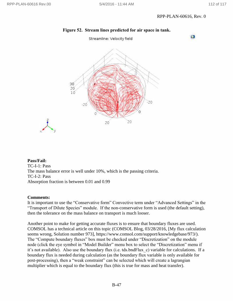
RPP-PLAN-60616, Rev. 0
B-47
Figure 52. Stream lines predicted for air space in tank.
Pass/Fail:
TC-I-1: Pass
The mass balance error is well under 10%, which is the passing criteria.
TC-I-2: Pass
Absorption fraction is between 0.01 and 0.99
Comments:
It is important to use the “Conservative form” Convective term under “Advanced Settings” in the
“Transport of Dilute Species” module. If the non-conservative form is used (the default setting),
then the tolerance on the mass balance on transport is much looser.
Another point to make for getting accurate fluxes is to ensure that boundary fluxes are used.
COMSOL has a technical article on this topic (COMSOL Blog, 03/28/2016, [My flux calculation
seems wrong, Solution number 973], https://www.comsol.com/support/knowledgebase/973/).
The “Compute boundary fluxes” box must be checked under “Discretization” on the module
node (click the eye symbol in “Model Builder” menu box to select the “Discretization” menu if
it’s not available). Also use the boundary flux (i.e. tds.bndFlux_c) variable for calculations. If a
boundary flux is needed during calculation (as the boundary flux variable is only available for
post-processing), then a “weak constraint” can be selected which will create a lagrangian
multiplier which is equal to the boundary flux (this is true for mass and heat transfer).
RPP-PLAN-60616 Rev.00 5/4/2016 - 11:44 AM 112 of 117

RPP-PLAN-60616, Rev. 0
B-48
It may be useful for problems like this where the flow field accuracy is much less important than
the concentration accuracy to scale the solver tolerances. This was not investigated in this study,
but is left as a tip for future work. The tolerance scaling can be adjusted manually (under
“Dependent Variable”. The automatic scaling adjusts the tolerance based on the magnitude of
the variable, not its importance to the modeling results.
COMSOL Report:
The model file is available in IDMS HISI Software Documentation folder for COMSOL as TC-I-
1.mph.
The report files is saved as word documents with the same case prefix in SmartPlant.
RPP-PLAN-60616 Rev.00 5/4/2016 - 11:44 AM 113 of 117

RPP-PLAN-60616, Rev. 0
B-49
Test Case ID: TC-J
Implementation Notes:
To get a more reasonable run time the flow calculations were done separately. This was done by
solving the air flow and natural convection in the liquid as steady state values, then using the
velocity values for the transient run. This is an approximation, but was deemed close enough for
this problem. The flow field was recalculated periodically as the mesh deformed. It’s possible
that instead of calculating the natural convection in the liquid that the “equivalent conductivity
for convection” method could have been used where the thermal conductivity of the liquid is
increased to account for the fluid movement, but this method was not pursued.
Results:
TC-J-1:
This model was run with diffusion only. If the flow field was added to the diffusion transport it
changed the surface concentration so that it couldn’t be compared with the hand calculation.
The calculated water concentration over the liquid is 1.4165 mol/m^3. This is a 1.6% deviation
from the hand calculated value of 1.44 mol/m^3. The difference is due to the saturation vapor
pressure which is calculated as 3533.3 Pa in COMSOL which is slightly lower than 3580 Pa
given by NIST (1.3% deviation, so the discrepancy due to how calculations are done is only
0.3%).
TC-J-2:
A two day time period is looked at, with a re-calculation of the flow field after the first day.
Integrating the boundary flux in time the following results are obtained.
Table 13. Water evaporation mass balance
2D Boundary integral
(mol/m)
Mass Balance Error
(%)
Inlet Interface Outlet
Day 1 -2587 -739 3326
Day 2 -2587 -760 3347
Total -5174 -1499 6672 0.00135
Assuming a 1 m depth to the 2D model, the interface water loss is 1499 mol over two days. This
would correspond to approximately 0.027 m^3 (1499mol * 18.02g/mol * 1kg/1000g *
1m^3/1000kg). The level change should be height=volume change/(length*width), which gives
0.054 m. The level change in COMSOL is 0.054 m which matches the hand calculation.
RPP-PLAN-60616 Rev.00 5/4/2016 - 11:44 AM 114 of 117
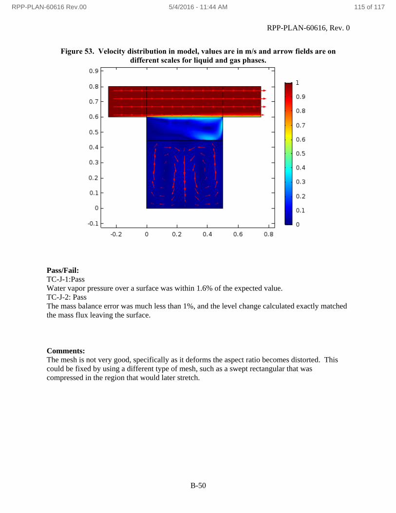
RPP-PLAN-60616, Rev. 0
B-50
Figure 53. Velocity distribution in model, values are in m/s and arrow fields are on
different scales for liquid and gas phases.
Pass/Fail:
TC-J-1:Pass
Water vapor pressure over a surface was within 1.6% of the expected value.
TC-J-2: Pass
The mass balance error was much less than 1%, and the level change calculated exactly matched
the mass flux leaving the surface.
Comments:
The mesh is not very good, specifically as it deforms the aspect ratio becomes distorted. This
could be fixed by using a different type of mesh, such as a swept rectangular that was
compressed in the region that would later stretch.
RPP-PLAN-60616 Rev.00 5/4/2016 - 11:44 AM 115 of 117

RPP-PLAN-60616, Rev. 0
B-51
Figure 54. Mesh after deformation. Note the elongated triangles in the upper half of the
middle region.
Laminar flow is probably a bad model to capture the step transition at the edge of the trench. It
was chosen to simplify computations.
A challenge with any model is to accomplish the desired simulation within the limitations of the
hardware computational ability. With COMSOL, most simple simulations using only one
physics module in 2D can run fairly quickly. Adding more physics or expanding to 3D add
complexity. Meshing seems to be a computationally intensive activity, and having the mesh
remade and a flow calculation redone slow down the solver. The solution in this instance was to
decouple those activities so that the flow or mesh deformation were solved on a specified
alternating schedule. Other simulations could use this technique, accept the computational time
of running both simultaneously, or devise some other method to simplify the solution and allow
for acceptable run times.
COMSOL Report:
The model files are available in IDMS HISI Software Documentation folder for COMSOL as
TC-I-1.mph and TC-I-2.mph.
The report files is saved as word documents with the same case prefix in SmartPlant.
RPP-PLAN-60616 Rev.00 5/4/2016 - 11:44 AM 116 of 117

RPP-PLAN-60616, Rev. 0
B-52
RPP-PLAN-60616 Rev.00 5/4/2016 - 11:44 AM 117 of 117
Top Related