Cambridge Working Paper Economics: 1710

DO SOVEREIGN WEALTH FUNDS DAMPEN THE NEGATIVE EFFECTS OF COMMODITY PRICE

VOLATILITY?

Kamiar Mohaddes

Mehdi Raissi

3 February 2017

This paper studies the impact of commodity terms of trade (CToT) volatility on economic growth (and its sources) in a sample of 69 commodity-dependent countries, and assesses the role of Sovereign Wealth Funds (SWFs) and quality of institutions in their long-term growth performance. Using annual data over the period 1981.2014, we employ the Cross-Sectionally augmented Autoregressive Distributive Lag (CS-ARDL) methodology for estimation to account for cross-country heterogeneity, cross-sectional dependence, and feedback effects. We find that while CToT volatility exerts a negative impact on economic growth (operating through lower accumulation of physical capital and lower TFP), the average impact is dampened if a country has a SWF and better institutional quality (hence a more stable government expenditure).

Cambridge Working Paper Economics

Faculty of Economics

Do Sovereign Wealth Funds Dampen the NegativeEffects of Commodity Price Volatility?∗

Kamiar Mohaddesa† and Mehdi Raissiba Faculty of Economics and Girton College, University of Cambridge, UK

and Centre for Applied Macroeconomic Analysis, ANU, Australiab International Monetary Fund, Washington DC, USA

February 2, 2017

Abstract

This paper studies the impact of commodity terms of trade (CToT) volatility oneconomic growth (and its sources) in a sample of 69 commodity-dependent countries,and assesses the role of Sovereign Wealth Funds (SWFs) and quality of institutions intheir long-term growth performance. Using annual data over the period 1981—2014, weemploy the Cross-Sectionally augmented Autoregressive Distributive Lag (CS-ARDL)methodology for estimation to account for cross-country heterogeneity, cross-sectionaldependence, and feedback effects. We find that while CToT volatility exerts a negativeimpact on economic growth (operating through lower accumulation of physical capitaland lower TFP), the average impact is dampened if a country has a SWF and betterinstitutional quality (hence a more stable government expenditure).

JEL Classifications: C23, E32, F43, O13, O40.Keywords: Economic growth, commodity prices, volatility, sovereign wealth funds.

∗Kamiar Mohaddes acknowledges financial support from the Economic Research Forum (ERF). Theviews expressed in this paper are those of the authors and do not necessarily represent those of the ERF,International Monetary Fund or IMF policy.†Corresponding author. Email address: km418@cam.ac.uk.

1 Introduction

Commodity-dependent countries are a heterogenous mix of high-, middle-, and low-income

countries that possess a large share of the world’s natural resources (around 90 percent

of crude oil reserves for example), and represent close to 20 percent of world GDP and

global exports. Natural resource wealth has enabled some of these countries to accumulate

substantial assets (placed in Sovereign Wealth Funds in a growing number of countries), and

provided a buffer against commodity-price shocks in several cases. However, not all resource-

rich countries have been able to leverage their assets to raise long-term economic growth due

to a number of factors, including pro-cyclical fiscal policies (especially in the Middle East),

underdeveloped public financial management frameworks, and fragile political systems. For

instance, Frankel et al. (2013) show that quality of institutions can play an important role in

making fiscal policy less pro-cyclical, hence making commodity wealth a blessing rather than

a curse. Moreover, when governments rely heavily on revenues derived from commodities,

they are subject to commodity price volatility, which if not managed properly, can result in

higher GDP growth volatility and disappointing long-term economic performance.1

This paper studies the impact of commodity price volatility on long-term economic growth

in a sample of 69 commodity-dependent countries over the period 1981—2014, and assesses

the role of Sovereign Wealth Funds (SWFs) and quality of institutions in shaping the growth

performance of these countries in the face of the extreme volatility in resource revenues

that they have experienced over time. The constructed Commodity Terms of Trade (CToT)

volatility measure is based on a monthly country-specific commodity-price index that de-

pends on the composition of a particular country’s commodity export- and import-baskets,

and is therefore weakly exogenous. Moreover, International Monetary Fund (2015) argues

that strong institutions and appropriate stabilization buffers can increase the chances of a

successful public investment scale-up, while Bahal et al. (2015) show that higher govern-

ment spending on infrastructure facilities (like roads, highways, and power) and/or health

and education may have a complementary impact on private sector investment by raising

the marginal productivity of private capital. We therefore also study the possible growth

channels– i.e. total factor productivity (TFP) and physical capital accumulation– through

which CToT volatility (and SWFs) affect long-term economic growth.

We employ the Cross-Sectionally augmented Autoregressive Distributive Lag (CS-ARDL)

approach for estimation to account for joint endogeneity of explanatory variables, cross-

country heterogeneity, and cross-sectional dependence. Accounting for these factors is par-

1For instance, over the 1981-2014 period GDP growth volatility in the Gulf Cooperation Council region(Bahrain, Kuwait, Oman, Qatar, Saudi Arabia, and the United Arab Emirates) has been at least three timeshigher than that of Chile and Norway.

1

ticularly important in our panel data analysis as the effect of commodity price volatility

on growth varies across cross-section units and depends critically on country-specific factors

(such as quality of institutions, level of economic and financial development, strength of pub-

lic financial management frameworks, and type of stabilization buffers) as well as feedback

effects from determinants of GDP growth. Moreover, controlling for observed characteris-

tics specific to countries alone need not ensure error cross-section independence. Neglecting

such dependencies can lead to biased estimates and spurious inference, particularly given

the rapid increase in globalization and exposures to global shocks.

Our results indicate that, on average, a highly-volatile CToT harms economic growth

of natural resource dependent countries in the long term. This is primarily due to price

volatility, which has been intrinsic in commodity markets. Nonetheless, there are significant

heterogeneities across countries– some economies have been able to grow strongly and sus-

tainably through multiple commodity price cycles (e.g. Chile and Norway), while many have

not. Trying to explain such a heterogeneity, our econometric results also show that having

a SWF, on average, can mitigate such negative growth effects, especially in countries that

enjoy higher-quality institutions (and hence less pro-cyclical fiscal policies). While we do

not explicitly model the impact of fiscal pro-cyclicality, International Monetary Fund (2015)

argues that countries with weak political institutions are more prone to wasteful spending

and pro-cyclical policies. Examining the channels through which these effects operate, we

find that CToT volatility is associated with lower accumulation of physical capital, lower

TFP, and thereby weaker growth. We show that long-term stabilization savings and sound

institutional frameworks are essential for dampening the negative effects of CToT volatility

via less frequent "stop-go" cycles in public investment and by enhancing productivity.

We are certainly not the first ones to emphasize the importance of volatility for economic

growth. Ramey and Ramey (1995) discuss the consequences of excess volatility for long-

run growth. Blattman et al. (2007) investigate the impact of terms of trade volatility

on the growth performance of 35 commodity-dependent countries between 1870 and 1939.

Aghion et al. (2009), using data on 83 countries over 1960—2000, show that higher levels

of exchange rate volatility can stunt growth, especially in countries with relatively under-

developed capital markets. Bleaney and Greenaway (2001) estimate a model for 14 sub-

Saharan African countries over 1980—1995 and show that growth is negatively affected by

terms of trade volatility, and investment by real exchange rate instability. van der Ploeg and

Poelhekke (2009, 2010) find that the volatility of unanticipated GDP growth has a negative

impact on economic growth, conditional on the country’s level of financial development.

Most closely related to our paper is Cavalcanti et al. (2015), who investigate the effects

of CToT volatility (σCToT ) on long-run economic growth of both commodity exporters and

2

importers. However, we rely on a higher frequency (and exogenously determined) measure

of σCToT , use a different estimation technique, and most importantly, have a different focus:

namely the role of SWFs and quality of institutions in mitigating the negative growth effects

of σCToT . While we do not explicitly control for other determinants of real GDP growth, the

country-specific intercepts, different short-run slope coeffi cients and error variances, as well

as cross-sectional averages of all the variables (as proxies for unobserved common factors) in

the CS-ARDL regressions capture the effects of such unobserved variables/factors.

The rest of the paper is organized as follows: Section 2 discusses the econometric model

and methodology; Section 3 presents the main results; and Section 4 concludes.

2 The Econometric Model and Methodology

We begin with the following panel data model that can nest much of the existing work on

the empirics of economic growth, from the "Barro cross-sectional regression" to the static

and dynamic panel data techniques:

∆yit = (φ− 1) yit−1 + β′xit + cyi + ηt + εit, (1)

for i = 1, 2, ..., N and t = 1, 2, ..., T

where ∆yit is the growth rate of real GDP per capita in country i; and yit−1 is the logarithm

of lagged real GDP per capita. xit is a vector of explanatory variables; ηt is the time-specific

effect; cyi is the country-specific effect; and εit is the error term. Within this framework, the

steady state output growth is exogenously determined by technological progress, while the

speed of adjustment toward the equilibrium is a function of the determinants of steady state

level of output and some initial conditions. Equation (1) allows one to study the potential

determinants of steady state level of output and test the conditional convergence hypothesis

in which countries converge to parallel equilibrium growth paths.

Much of the empirical growth literature is based on estimations of equation (1) using

a cross-sectional approach or fixed/random effects panel estimators. Cross-sectional regres-

sions clearly suffer from endogeneity problems as by construction, the initial level of income,

yit−1, is correlated with the error term, εit. This endogeneity bias is larger when considering

the simultaneous determination of virtually all growth determinants, and the correlation of

unobserved country-specific factors (arising from global shocks) and the explanatory vari-

ables. Traditional static panel data estimators such as fixed and random effects are not

consistent either, due to the inclusion of lagged dependent variables in regressions (e.g.

the initial level of GDP per capita). Specifically, the fixed effects estimator is inconsistent

3

because it usually eliminates cyi by a de-meaning transformation that induces a negative

correlation between the transformed error and the lagged dependent variables of order 1/T ,

which in short panels remains substantial. The assumption of a lack of correlation between

cyi and the explanatory variables required for random effects consistency is also violated as

both ∆yit and yit−1 are functions of cyi. These estimators (or their standard errors) will be

biased if the errors show either heteroscedasticity or serial correlation.

We specify our growth regression dynamically and include lagged GDP per capita on the

right hand side. Hence, the elimination of fixed effects from equation (1) in any standard

OLS-based estimation procedure implies the violation of the orthogonality condition between

the error term and explanatory variables. For this reason, we estimate this equation using

the CS-ARDL approach. While a system GMM estimator can effectively deal with the

endogeneity problem and country-specific fixed effects, it restricts all the slope coeffi cients

to be identical across countries; assumes that the time effects are homogenous; and that the

errors are cross-sectionally independent. If any of these conditions are not satisfied, the GMM

method can produce inconsistent estimates of the average values of parameters; see Pesaran

and Smith (1995) for more details. The time-specific heterogeneity is an underestimated but

at the same time very important concern in dynamic panel data models. Country-specific

time-effects can capture a number of unobservable characteristics in macroeconomic and

financial applications such as (a) institutional arrangements, (b) the patterns of trade, and

(c) political developments. The time-specific heterogeneity is induced by oil price shocks,

the stance of global financial cycles, and/or other global common factors, which affect all

countries but to different degrees. The CS-ARDL methodology explained below accounts

for heterogenous time effects and deals with cross-sectional dependencies effectively.

2.1 CS-ARDL Methodology

When panels of data are available, there exist a number of alternative estimation methods

that vary on the extent to which they account for parameter heterogeneity. At one extreme

is the Mean Group (MG) approach in which separate equations are estimated for each

country and the average of estimated coeffi cients across countries is examined. Pesaran and

Smith (1995) show that the MG method produces consistent estimates of the average of the

parameters when the time-series dimension of the data is suffi ciently large. At the other

extreme are the traditional estimators in which dynamics are simply pooled and treated

as homogeneous. Prominent examples include fixed effects (FE), random effects (RE), and

generalized methods of moments (GMM). In between the two extremes is the pooled mean

group (PMG) estimator of Pesaran and Shin (1999) which is an intermediate case between the

4

averaging and pooling methods of estimation, and involves aspects of both. It restricts the

long-run coeffi cients to be homogenous over the cross-sections, but allows for heterogeneity

in intercepts, short-run coeffi cients (including the speed of adjustment) and error variances.

The PMG estimator also generates consistent estimates of the mean of short-run coeffi cients

across countries by taking the simple average of individual country coeffi cients.

We use the Cross-Sectionally augmented Autoregressive Distributive Lag (CS-ARDL)

methodology of Chudik and Pesaran (2015) and Chudik et al. (2016a) to estimate, and

report the pooled long-run estimates based on the PMG estimator because it offers the

best available choice in terms of consistency and effi ciency in our sample.2 The CS-ARDL

method avoids the need for pre-testing the order of integration given that they are valid

whether the variables of interest are I(0) or I(1). It is also robust to omitted variables bias

and simultaneous determination of growth regressors. The main requirements for the validity

of this methodology are that, first, there exists a long-run relationship among the variables of

interest and, second, the dynamic specification of the model is suffi ciently augmented so that

the regressors become weakly exogenous and the resulting residual is serially uncorrelated.

To explain the CS-ARDL estimator in detail, consider the following panel ARDL(1, ..., 1)

model with a multifactor error structure:

yit = cyi + φiyi,t−1 + β′0ixit + β′1ixi,t−1 + uit, (2)

uit = γ ′ift + εit, (3)

ωit =

(xit

git

)= cωi +αiyi,t−1 + Γ′ift + vit, (4)

where as before i = 1, 2, ..., N, t = 1, 2, ..., T , and xit is kx × 1 vector of regressors specific to

cross-section unit i at time t; cyi and cωi are individual fixed effects for unit i, git is kg × 1

vector of covariates specific to unit i (not observed in the panel data model), kx + kg = k,

εit are the idiosyncratic errors, Γi is an m × k matrix of factor loadings (k ≥ m), αiis a k × 1 vector of unknown coeffi cients, and vit is assumed to follow a general linear

covariance stationary process distributed independently of εit, the idiosyncratic errors. ft is

anm×1 vector of unobserved common factors, which can be stationary or nonstationary; see

Kapetanios et al. (2011). The source of error term dependencies across countries is captured

by ft, whereas the impacts of these factors on each country are governed by the idiosyncratic

loadings in Γi. The individual-specific errors, εit, are distributed independently across i and

t; they are not correlated with the unobserved common factors or the regressors; and they

have zero mean, variance greater than zero, and finite fourth moments. The unobserved

2See also Chudik et al. (2013) and Chudik et al. (2016b) for other applications of the CS-ARDL method.

5

common factors, or the heterogenous time effects, may be captured/proxied by adding cross-

sectional averages of the observables to our regressions, see Pesaran (2006) and Chudik and

Pesaran (2015).3

Assuming that N is suffi ciently large, Chudik and Pesaran (2015) show that the un-

observed common factors, ft, can be proxied by de-trended cross-section averages of zit =

(yit,x′it,g

′it)′ and their lags:

ft = G (L) zwt +Op(N−1/2), (5)

where G (L) is a distributed lag function, zwt = zwt − czw is a k + 1 dimensional vector of

de-trended cross-section averages, zwt = (ywt,x′wt,g

′wt)′ =

∑Ni=1wizit is a k + 1 dimensional

vector of cross-section averages, and czw =∑N

i=1wi (Ik+1 −Ai)−1 czi. The weights satisfy

the following normalization condition:∑N

i=1wi = 1.

Substituting (5) into (2), we obtain

yit = c∗yi + φiyi,t−1 + β′0ixit + β′1ixi,t−1 + δ′i (L) zwt + εit +Op(N−1/2), (6)

where

δi (L) =∞∑`=0

δi`L` = G′ (L)γi, (7)

and c∗yi = cyi − δ′i (1) czw.

Equation (2) can be estimated using the MG and PMG estimators, however, for the

estimators to be valid, a suffi cient number of lags of cross-section averages must be included

in individual equations of the panel (as we truncate the infinite polynomial distributed lag

function δi (L)), and the number of cross-section averages must be at least as large as the

number of unobserved common factors. Moreover, as always T must be large enough so that

the model can be estimated for each cross-section unit.

The estimated MG vector is defined as θ =E(θi),where the individual long-run or level

coeffi cients are

θi =β0i + β1i

1− φi. (8)

To obtain the PMG estimates, the individual long-run coeffi cients are restricted to be the

3Conditioning on observed variables (growth regressors) specific to countries alone need not ensure errorcross-section independence that underlies much of the panel data literature. Neglecting such dependenciescan lead to biased estimates and spurious inference, particularly given the rapid increase in world trade,international financial linkages, and exposures to common shocks.

6

same across countries, namely:

θi = θ, i = 1, 2, ..., N. (9)

The PMG estimator uses a maximum likelihood approach to estimate the model based

on the Newton—Raphson algorithm.

3 Empirical Results

To empirically test the relationship between economic growth and commodity terms of trade

(CToT) growth, gCToT , and volatility, σCToT , we use annual data from 1980 to 2014 on: real

GDP per capita, a CToT index based on the prices of 45 primary commodities, a dummy

variable that takes the value of one if a country has a SWF, and a measure of institutional

quality. To investigate the possible mechanisms through which CToT volatility can harm

economic growth, we focus on: (i) TFP growth; and (ii) physical capital accumulation. We

obtain the data on real GDP, capital stock, and TFP from the Penn World Table Version 9.0

database and the institutional quality data from the Political Risk Services Group databases.

As in Spatafora and Tytell (2009), we define a country-specific measure of the CToT

index as:

CToTiτ =∏j

(Pjτ

MUVτ

)Xij/∏j

(Pjτ

MUVτ

)Mij

, (10)

where MUVτ is a manufacturing unit value index used as deflator, Xij (Mij) is the share

of exports (imports) of commodity j in country i’s GDP, and Pjτ is the individual com-

modity price in month τ . We construct this monthly index based on data (on the prices

of 45 primary commodities) obtained from the International Monetary Fund International

Financial Statistics databases. Note that by construction, the movements in the CToT in-

dex are due to changes in commodity prices as the export and import shares are taken to

be constant over time (i.e. long-term averages). The CToT index (10) allows countries to

be influenced by changes in commodity prices differently, depending on the composition of

their export and import baskets. This is in contrast to the "standard" commodity price

indices most commonly used in the literature, such as the "All Primary Commodities Index"

in International Monetary Fund (2012), which attaches the same weight to each country in

the regression analysis. Equation (10) is then used to construct two important variables.

The first is an annual CToT growth series, gCToT,it, which is calculated in two steps: (i)

year-on-year growth rate of the monthly CToT index is taken, and (ii) the average over the

year is calculated. The second is a measure of realized CToT volatility for year t, σCToT,it,

7

which is constructed as the standard deviation of the year-on-year growth rates of CToTiτduring months τ = 1, ..., 12 in year t. Therefore, in contrast to most studies in the growth

literature which employ time-invariant measures of volatility, we construct a time-varying

measure of commodity price volatility, σCToT,it.

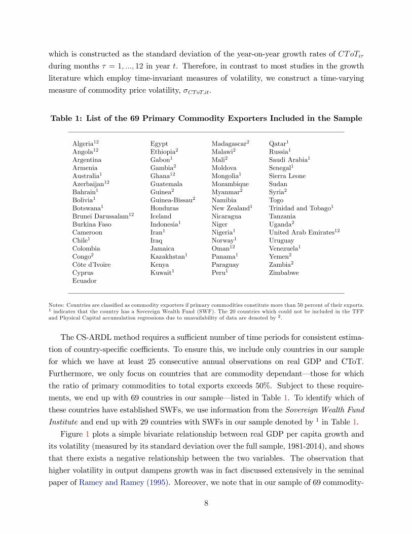
Table 1: List of the 69 Primary Commodity Exporters Included in the Sample

Algeria12 Egypt Madagascar2 Qatar1

Angola12 Ethiopia2 Malawi2 Russia1

Argentina Gabon1 Mali2 Saudi Arabia1

Armenia Gambia2 Moldova Senegal1

Australia1 Ghana12 Mongolia1 Sierra LeoneAzerbaijan12 Guatemala Mozambique SudanBahrain1 Guinea2 Myanmar2 Syria2

Bolivia1 Guinea-Bissau2 Namibia TogoBotswana1 Honduras New Zealand1 Trinidad and Tobago1

Brunei Darussalam12 Iceland Nicaragua TanzaniaBurkina Faso Indonesia1 Niger Uganda2

Cameroon Iran1 Nigeria1 United Arab Emirates12

Chile1 Iraq Norway1 UruguayColombia Jamaica Oman12 Venezuela1

Congo2 Kazakhstan1 Panama1 Yemen2

Côte d’Ivoire Kenya Paraguay Zambia2

Cyprus Kuwait1 Peru1 ZimbabweEcuador

Notes: Countries are classified as commodity exporters if primary commodities constitute more than 50 percent of their exports.1 indicates that the country has a Sovereign Wealth Fund (SWF). The 20 countries which could not be included in the TFPand Physical Capital accumulation regressions due to unavailability of data are denoted by 2.

The CS-ARDL method requires a suffi cient number of time periods for consistent estima-

tion of country-specific coeffi cients. To ensure this, we include only countries in our sample

for which we have at least 25 consecutive annual observations on real GDP and CToT.

Furthermore, we only focus on countries that are commodity dependant– those for which

the ratio of primary commodities to total exports exceeds 50%. Subject to these require-

ments, we end up with 69 countries in our sample– listed in Table 1. To identify which of

these countries have established SWFs, we use information from the Sovereign Wealth Fund

Institute and end up with 29 countries with SWFs in our sample denoted by 1 in Table 1.

Figure 1 plots a simple bivariate relationship between real GDP per capita growth and

its volatility (measured by its standard deviation over the full sample, 1981-2014), and shows

that there exists a negative relationship between the two variables. The observation that

higher volatility in output dampens growth was in fact discussed extensively in the seminal

paper of Ramey and Ramey (1995). Moreover, we note that in our sample of 69 commodity-

8

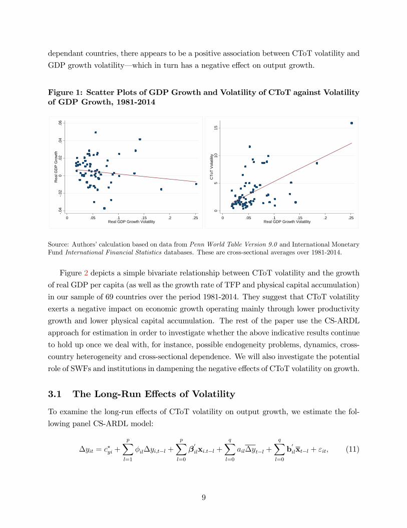
dependant countries, there appears to be a positive association between CToT volatility and

GDP growth volatility– which in turn has a negative effect on output growth.

Figure 1: Scatter Plots of GDP Growth and Volatility of CToT against Volatilityof GDP Growth, 1981-2014

­.04

­.02

0.0

2.0

4.0

6R

eal G

DP 

Gro

wth

0 .05 .1 .15 .2 .25Real GDP Growth Volatility

05

1015

CTo

T Vo

latil

ity0 .05 .1 .15 .2 .25

Real GDP Growth Volatility

Source: Authors’calculation based on data from Penn World Table Version 9.0 and International MonetaryFund International Financial Statistics databases. These are cross-sectional averages over 1981-2014.

Figure 2 depicts a simple bivariate relationship between CToT volatility and the growth

of real GDP per capita (as well as the growth rate of TFP and physical capital accumulation)

in our sample of 69 countries over the period 1981-2014. They suggest that CToT volatility

exerts a negative impact on economic growth operating mainly through lower productivity

growth and lower physical capital accumulation. The rest of the paper use the CS-ARDL

approach for estimation in order to investigate whether the above indicative results continue

to hold up once we deal with, for instance, possible endogeneity problems, dynamics, cross-

country heterogeneity and cross-sectional dependence. We will also investigate the potential

role of SWFs and institutions in dampening the negative effects of CToT volatility on growth.

3.1 The Long-Run Effects of Volatility

To examine the long-run effects of CToT volatility on output growth, we estimate the fol-

lowing panel CS-ARDL model:

∆yit = c∗yi +

p∑l=1

φil∆yi,t−l +

p∑l=0

β′

ilxi.t−l +

q∑l=0

ail∆yt−l +

q∑l=0

b′

ilxt−l + εit, (11)

9

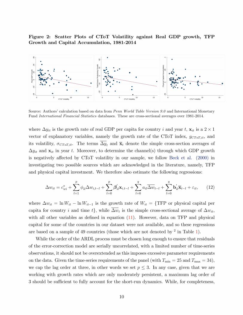
Figure 2: Scatter Plots of CToT Volatility against Real GDP growth, TFPGrowth and Capital Accumulation, 1981-2014

­.04

­.02

0.0

2.0

4.0

6R

eal G

DP 

Gro

wth

0 5 10 15CToT Volatility

­.02

­.01

0.0

1.0

2To

tal F

acto

r Pro

duct

ivity

 Gro

wth

0 5 10 15CToT Volatility

­.05

0.0

5.1

Phys

ical

 Cap

ital A

ccum

ulat

ion

0 5 10 15CToT Volatility

Source: Authors’calculation based on data from Penn World Table Version 9.0 and International MonetaryFund International Financial Statistics databases. These are cross-sectional averages over 1981-2014.

where ∆yit is the growth rate of real GDP per capita for country i and year t, xit is a 2× 1

vector of explanatory variables, namely the growth rate of the CToT index, gCToT,it, and

its volatility, σCToT,it. The terms ∆yt and xt denote the simple cross-section averages of

∆yit and xit in year t. Moreover, to determine the channel(s) through which GDP growth

is negatively affected by CToT volatility in our sample, we follow Beck et al. (2000) in

investigating two possible sources which are acknowledged in the literature, namely, TFP

and physical capital investment. We therefore also estimate the following regressions:

∆wit = c∗wi +

p∑l=1

φil∆wi,t−l +

p∑l=0

β′

ilxi.t−l +

q∑l=0

ail∆wt−l +

q∑l=0

b′

ilxt−l + εit, (12)

where ∆wit = lnWit − lnWit−1 is the growth rate of Wit = {TFP or physical capital percapita for country i and time t}, while ∆wt is the simple cross-sectional average of ∆wit,

with all other variables as defined in equation (11). However, data on TFP and physical

capital for some of the countries in our dataset were not available, and so these regressions

are based on a sample of 49 countries (those which are not denoted by 2 in Table 1).

While the order of the ARDL process must be chosen long enough to ensure that residuals

of the error-correction model are serially uncorrelated, with a limited number of time-series

observations, it should not be overextended as this imposes excessive parameter requirements

on the data. Given the time-series requirements of the panel (with Tmin = 25 and Tmax = 34),

we cap the lag order at three, in other words we set p ≤ 3. In any case, given that we are

working with growth rates which are only moderately persistent, a maximum lag order of

3 should be suffi cient to fully account for the short-run dynamics. While, for completeness,

10

we report the results for p = 1, 2, and 3, we mainly rely on those with p = 3.

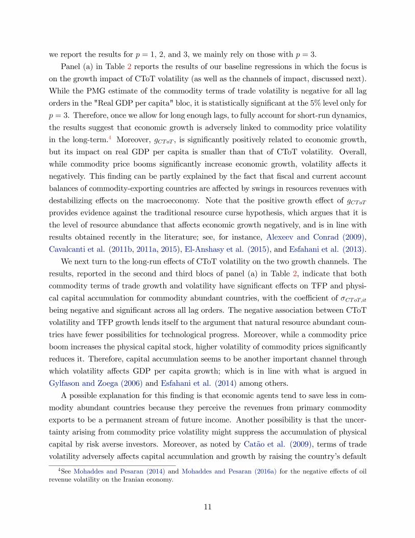
Panel (a) in Table 2 reports the results of our baseline regressions in which the focus is

on the growth impact of CToT volatility (as well as the channels of impact, discussed next).

While the PMG estimate of the commodity terms of trade volatility is negative for all lag

orders in the "Real GDP per capita" bloc, it is statistically significant at the 5% level only for

p = 3. Therefore, once we allow for long enough lags, to fully account for short-run dynamics,

the results suggest that economic growth is adversely linked to commodity price volatility

in the long-term.4 Moreover, gCToT , is significantly positively related to economic growth,

but its impact on real GDP per capita is smaller than that of CToT volatility. Overall,

while commodity price booms significantly increase economic growth, volatility affects it

negatively. This finding can be partly explained by the fact that fiscal and current account

balances of commodity-exporting countries are affected by swings in resources revenues with

destabilizing effects on the macroeconomy. Note that the positive growth effect of gCToTprovides evidence against the traditional resource curse hypothesis, which argues that it is

the level of resource abundance that affects economic growth negatively, and is in line with

results obtained recently in the literature; see, for instance, Alexeev and Conrad (2009),

Cavalcanti et al. (2011b, 2011a, 2015), El-Anshasy et al. (2015), and Esfahani et al. (2013).

We next turn to the long-run effects of CToT volatility on the two growth channels. The

results, reported in the second and third blocs of panel (a) in Table 2, indicate that both

commodity terms of trade growth and volatility have significant effects on TFP and physi-

cal capital accumulation for commodity abundant countries, with the coeffi cient of σCToT,itbeing negative and significant across all lag orders. The negative association between CToT

volatility and TFP growth lends itself to the argument that natural resource abundant coun-

tries have fewer possibilities for technological progress. Moreover, while a commodity price

boom increases the physical capital stock, higher volatility of commodity prices significantly

reduces it. Therefore, capital accumulation seems to be another important channel through

which volatility affects GDP per capita growth; which is in line with what is argued in

Gylfason and Zoega (2006) and Esfahani et al. (2014) among others.

A possible explanation for this finding is that economic agents tend to save less in com-

modity abundant countries because they perceive the revenues from primary commodity

exports to be a permanent stream of future income. Another possibility is that the uncer-

tainty arising from commodity price volatility might suppress the accumulation of physical

capital by risk averse investors. Moreover, as noted by Catão et al. (2009), terms of trade

volatility adversely affects capital accumulation and growth by raising the country’s default

4See Mohaddes and Pesaran (2014) and Mohaddes and Pesaran (2016a) for the negative effects of oilrevenue volatility on the Iranian economy.

11

risk, hence widening the country spreads, and lowering its borrowing capacity.

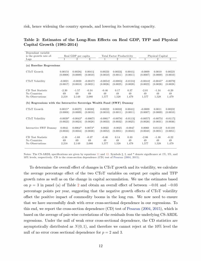
Table 2: Estimates of the Long-Run Effects on Real GDP, TFP and PhysicalCapital Growth (1981-2014)

Dependant variableis the growth rate of: Real GDP per capita Total Factor Productivity Physical CapitalLags 1 2 3 1 2 3 1 2 3

(a) Baseline Regressions

CToT Growth 0.0015† 0.0028‡ 0.0041‡ 0.0023† 0.0033‡ 0.0041‡ -0.0009 0.0010 0.0022†(0.0008) (0.0009) (0.0010) (0.0010) (0.0011) (0.0011) (0.0007) (0.0009) (0.0010)

CToT Volatility -0.0021 -0.0020 -0.0047† -0.0054† -0.0085‡ -0.0124‡ -0.0044† -0.0045* -0.0079‡(0.0017) (0.0018) (0.0021) (0.0026) (0.0025) (0.0020) (0.0022) (0.0026) (0.0028)

CD Test Statistic -2.30 -1.57 -0.34 -0.46 0.17 0.37 -2.01 -1.34 -0.20No Countries 69 69 69 49 49 49 49 49 49No Observations 2,218 2,149 2,080 1,577 1,528 1,479 1,577 1,528 1,479

(b) Regressions with the Interactive Sovereign Wealth Fund (SWF) Dummy

CToT Growth 0.0015* 0.0027‡ 0.0038‡ 0.0022† 0.0033‡ 0.0041‡ -0.0009 0.0011 0.0023†(0.0008) (0.0009) (0.0010) (0.0010) (0.0011) (0.0011) (0.0007) (0.0009) (0.0010)

CToT Volatility -0.0039* -0.0043* -0.0067† -0.0061* -0.0078† -0.0113‡ -0.0057† -0.0075† -0.0117‡(0.0023) (0.0024) (0.0028) (0.0033) (0.0032) (0.0025) (0.0026) (0.0031) (0.0036)

Interactive SWF Dummy 0.0041 0.0064* 0.0073* 0.0022 -0.0025 -0.0047 0.0060 0.0112† 0.0110†(0.0033) (0.0034) (0.0038) (0.0052) (0.0051) (0.0045) (0.0048) (0.0051) (0.0051)

CD Test Statistic -2.38 -1.68 -0.37 -0.46 0.14 0.33 -2.06 -1.38 -0.22No Countries 69 69 69 49 49 49 49 49 49No Observations 2,218 2,149 2,080 1,577 1,528 1,479 1,577 1,528 1,479

Notes: The CS-ARDL specifications are given by equations 11 and 12. Symbols ‡, †, and * denote significance at 1%, 5%, and10% levels, respectively. CD is the cross-section dependence (CD) test of Pesaran (2004, 2015).

To determine the overall effect of changes in CToT growth and its volatility, we calculate

the average percentage effect of the two CToT variables on output per capita and TFP

growth rates as well as on the change in capital accumulation. We use the estimates based

on p = 3 in panel (a) of Table 2 and obtain an overall effect of between −0.01 and −0.03

percentage points per year, suggesting that the negative growth effects of CToT volatility

offset the positive impact of commodity booms in the long run. We now need to ensure

that we have successfully dealt with error cross-sectional dependence in our regressions. To

this end, we report the cross-section dependence (CD) test of Pesaran (2004, 2015), which is

based on the average of pair-wise correlations of the residuals from the underlying CS-ARDL

regressions. Under the null of weak error cross-sectional dependence, the CD statistics are

asymptotically distributed as N(0, 1), and therefore we cannot reject at the 10% level the

null of no error cross sectional dependence for p = 2 and 3.

12

Finally, as we expect the long-run growth effects of CToT volatility for primary commod-

ity exporters to be different from those countries that are not dependant on a handful of

primary products, we run the same regressions as in (11) but for a sample 61 countries that

have a more diversified export basket. The results for these 61 countries show that CToT

volatility is not significantly related to economic growth in the long-run. This is mainly be-

cause these countries have a more diversified basket of exports, especially manufacturing or

service-sector goods, and so they are expected to grow faster and be better insured against

price fluctuations in individual commodities. This is in contrast to the experience of the

sample of 69 primary product exporters in Table 2, for which our results indicate that higher

CToT volatility harms growth. The results for the sample of 61 diversified countries are not

reported here, but are available upon request.5

3.2 The Role of SWFs and Institutional Quality

While many SWFs have been in existence for over half a century (such as the Kuwait Invest-

ment Authority which was founded in 1953), a large number of funds have been established

(by major commodity exporters in particular) over the last two decades. These SWFs accu-

mulated large assets during the most recent oil-price boom (2002—2008), have played a major

role in reserve management of commodity revenues, and contributed to macroeconomic sta-

bilization in several cases. SWFs have been established for a variety of reasons, ranging from

fiscal stabilization (that is to help smooth the impact on government spending of revenues

that are large and volatile), to long-term saving for future needs of the economy, or of specific

groups such as pensioners, or for future generations. One of the main short-term objectives

of SWFs is to counter the adverse macroeconomic effects of commodity price volatility. We

next investigate whether SWFs have been successful, on average, in fulfilling this objective.

Using data from the Sovereign Wealth Fund Institute, we identify 29 countries in our

sample as having established SWFs. These are denoted by 1 in Table 1. 19 of these are

funded by revenue from exports of crude oil and gas, of which ten are members of the

Organization of the Petroleum Exporting Countries (OPEC), and seven are located in the

Persian Gulf. It is estimated by the Sovereign Wealth Fund Institute that in late 2016 the

total assets of SWFs were around $7.5 trillion with over 60% of these being funded by oil

and gas exports. The prominent examples are Norway’s Government Pension Fund ($830),

Abu Dhabi Investment Authority ($773), Saudi Arabia’s Fund (SAMA) ($685), Kuwait

Investment Authority ($592), and Qatar Investment Authority ($256), with the number in

5The asymmetric effects of CToT volatility on GDP growth in the two country groups considered (com-modity dependant and more diversified countries) is also supported by the results in Cavalcanti et al. (2015).

13

brackets referring to their market values in billions in June 2015.6

To examine the role of SWFs in mitigating the negative growth effects of CToT volatility

and the channels of impact, we add an interactive SWF dummy, (SWF × σCToT,it) whereSWF takes the value of unity if a country has established a SWF and zero otherwise, to

the vector of explanatory variables, xit, in equation (11). The results are reported in panel

(b) of Table 2. As before, the long-run effects of σCToT,it is negative for real GDP per capita

growth and the channels of impact are lower TFP and physical capital accumulation. Note

also that the coeffi cient of CToT volatility is negative and statistically significant for all

lag orders. More importantly, the estimated coeffi cient of the interactive SWF dummy is

positive and statistically significant in the first and third blocs. In other words, countries that

have a SWF in our sample have, on average, performed better when it comes to mitigating

the negative growth effects of CToT volatility and managed to sustain a higher level of

capital accumulation in the face of the extreme volatility in resource revenues. Our results,

therefore, suggests that one is better able to dampen the negative long-run growth effects of

CToT volatility with a well-functioning SWF that can effectively deal with the adverse effects

of (excess) commodity price volatility– add to the fund when commodity prices are high and

transfer less to it or even withdraw from it when prices are low to smooth expenditure.

For instance, oil exporters in the Persian Gulf, enjoyed a large increase in their SWFs

assets while oil prices were high for most of the past decade, but more recently many of

them have dipped into their SWFs following the collapse in oil prices since 2014.7 Rather

than cutting back on public expenditure (social welfare programs, public salaries, and in-

frastructure spending), many governments either withdrew money from their funds (such as

Russia and Saudi Arabia) or alternatively transferred less revenue to these funds. To give

a concrete example, since 1976 the Kuwaiti government has by law transferred a minimum

of 10 percent of all state revenues to the Future Generation Fund (FGF). However, with oil

prices having been high for almost a decade it was announced in March 2013, following an

Amir budgetary decree, that the minimum contribution is to be increased to 25 percent. But

the following year oil prices fell sharply and remained low, and so the decision was reversed

and the contribution to the FGF was cut back to 10 percent from fiscal year 2015/16.

We next check the robustness of our results to the definition of SWF and re-estimate

our growth regressions (11) excluding the seven countries whose SWFs are mainly funded by

non-commodity revenues (Australia, Bolivia, Indonesia, New Zealand, Panama, Peru, and

6Note that given the objective of these funds, on average 65% of the SWF assets are held in public andprivate equities (61% Norway; 72% SAMA; 65% Kuwait; 68% Qatar; 62% Abu Dhabi—figures based on 2014).See Mohaddes and Pesaran (2016b) for more details.

7See also Mohaddes and Raissi (2015) who quantify the global macroeconomic consequences of falling oilprices due to the oil revolution in the United States.

14

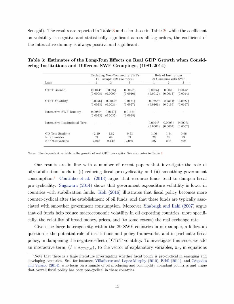
Senegal). The results are reported in Table 3 and echo those in Table 2: while the coeffi cient

on volatility is negative and statistically significant across all lag orders, the coeffi cient of

the interactive dummy is always positive and significant.

Table 3: Estimates of the Long-Run Effects on Real GDP Growth when Consid-ering Institutions and Different SWF Groupings, (1981-2014)

Excluding Non-Commodity SWFs Role of InstitutionsFull sample (69 Countries) 29 Countries with SWF

Lags 1 2 3 1 2 3

CToT Growth 0.0014* 0.0025‡ 0.0035‡ 0.0025† 0.0020 0.0026*(0.0008) (0.0009) (0.0010) (0.0012) (0.0013) (0.0014)

CToT Volatility -0.0056† -0.0069‡ -0.0124‡ -0.0283* -0.0364† -0.0527‡(0.0023) (0.0024) (0.0027) (0.0161) (0.0169) (0.0167)

Interactive SWF Dummy 0.0080† 0.0127‡ 0.0167‡ - - -(0.0033) (0.0035) (0.0038)

Interactive Institutional Term - - - 0.0004* 0.0005† 0.0007‡(0.0002) (0.0002) (0.0002)

CD Test Statistic -2.49 -1.82 -0.53 1.06 0.54 -0.06No Countries 69 69 69 29 29 29No Observations 2,218 2,149 2,080 927 898 869

Notes: The dependant variable is the growth of real GDP per capita. See also notes to Table 2.

Our results are in line with a number of recent papers that investigate the role of

oil/stabilization funds in (i) reducing fiscal pro-cyclicality and (ii) smoothing government

consumption.8 Coutinho et al. (2013) argue that resource funds tend to dampen fiscal

pro-cyclicality. Sugawara (2014) shows that government expenditure volatility is lower in

countries with stabilization funds. Koh (2016) illustrates that fiscal policy becomes more

counter-cyclical after the establishment of oil funds, and that these funds are typically asso-

ciated with smoother government consumption. Moreover, Shabsigh and Ilahi (2007) argue

that oil funds help reduce macroeconomic volatility in oil exporting countries, more specifi-

cally, the volatility of broad money, prices, and (to some extent) the real exchange rate.

Given the large heterogeneity within the 29 SWF countries in our sample, a follow-up

question is the potential role of institutions and policy frameworks, and in particular fiscal

policy, in dampening the negative effect of CToT volatility. To investigate this issue, we add

an interactive term, (I × σCToT,it) , to the vector of explanatory variables, xit, in equations8Note that there is a large literature investigating whether fiscal policy is pro-cyclical in emerging and

developing countries. See, for instance, Villafuerte and Lopez-Murphy (2010), Erbil (2011), and Céspedesand Velasco (2014), who focus on a sample of oil producing and commodity abundant countries and arguethat overall fiscal policy has been pro-cyclical in these countries.

15

(11). I is based on data from the Political Risk Services Group databases, measuring the

average quality of institutions between 1984-2012, and takes a value between 0 and 100.

The results are reported in the second block of Table 3, and perhaps not surprisingly,

illustrate that within the SWF sample, countries with stronger institutions, have been better

able to mitigate the negative growth effects of CToT volatility. Note that the coeffi cient of

σCToT,it is negative and significant for all lag orders, while the coeffi cient of the interactive

institutional quality term is positive and statistically significant for p = 1, 2, and 3. These

results are in line with Frankel et al. (2013), who argue that the better institutions in devel-

oping countries are, the more likely they are to pursue less procyclical or more countercyclical

fiscal policy, as well as Sugawara (2014) who shows that the two significant factors in reduc-

ing government expenditure volatility are stronger institutions and fiscal rules. Overall, our

results suggest that while volatility represents a fundamental barrier to economic prosper-

ity, the establishment of SWFs, as well as appropriate institutions, can help mitigating the

negative effects. Therefore, creating a mechanism of short-term management of commodity

price volatility through stabilization funds should be a priority for commodity dependant

countries, complemented by well-functioning public financial management systems.

4 Concluding Remarks

This paper contributed to the literature by examining empirically the effects of commodity

price booms and CToT volatility on GDP per capita growth and its sources. We created an

annual panel dataset and used the CS-ARDL approach to account for endogeneity, cross-

country heterogeneity, and cross-sectional dependence which arise from unobserved common

factors. The main finding was that while CToT growth enhances real output per capita,

CToT volatility exerts a negative impact on economic growth operating through lower ac-

cumulation of physical capital and lower TFP. Our econometric results also showed that,

on average, having a SWF can mitigate such negative growth effects, especially in countries

that enjoy higher-quality institutions (and hence less pro-cyclical fiscal policies).

Our results have strong policy implications. The undesirable consequences of commodity

price volatility can be avoided if resource-rich countries are able to improve the management

of volatility in resource income by setting up forward-looking institutions such as Sovereign

Wealth Funds, or adopting short-term mechanisms such as stabilization funds with the aim

of saving when commodity prices are high and spending accumulated revenues when prices

are low. The government can also intervene in the economy by increasing public capital

expenditure when private investment is low, using proceeds from the stabilization fund.

Alternatively the government can use these funds to increase the complementarities of phys-

16

ical and human capital, such as improving the judicial system, property rights, and human

capital. This would increase the returns on investment with positive effects on capital accu-

mulation, TFP, and growth. Improving the functioning of financial markets is also a crucial

step as this allows firms and households to insure against shocks, decreasing uncertainty and

therefore mitigating the negative effects of volatility on investment and economic growth.

17

References

Aghion, P., P. Bacchetta, R. Rancière, and K. Rogoff (2009). Exchange Rate Volatility

and Productivity Growth: The Role of Financial Development. Journal of Monetary Eco-

nomics 56 (4), 494—513.

Alexeev, M. and R. Conrad (2009). The Elusive Curse of Oil. The Review of Economics

and Statistics 91 (3), 586—598.

Bahal, G., M. Raissi, and V. Tulin (2015). Crowding-Out or Crowding-In? Public and

Private Investment in India . IMF Working Paper WP/15/264 .

Beck, T., R. Levine, and N. Loayza (2000). Finance and the Sources of Growth. Journal

of Financial Economics 58 (1-2), 261—300.

Blattman, C., J. Hwang, and J. G. Williamson (2007). Winners and Losers in the Com-

modity Lottery: The Impact of Terms of Trade Growth and Volatility in the Periphery

1870-1939. Journal of Development Economics 82 (1), 156—179.

Bleaney, M. and D. Greenaway (2001). The Impact of Terms of Trade and Real Exchange

Rate Volatility on Investment and Growth in Sub-Saharan Africa. Journal of Development

Economics 65 (2), 491—500.

Catão, L. A. V., A. Fostel, and S. Kapur (2009). Persistent Gaps and Default Traps.

Journal of Development Economics 89 (2), 271—284.

Cavalcanti, T. V. d. V., K. Mohaddes, and M. Raissi (2011a). Growth, Development and

Natural Resources: New Evidence Using a Heterogeneous Panel Analysis. The Quarterly

Review of Economics and Finance 51 (4), 305—318.

Cavalcanti, T. V. d. V., K. Mohaddes, and M. Raissi (2011b). Does Oil Abundance Harm

Growth? Applied Economics Letters 18 (12), 1181—1184.

Cavalcanti, T. V. D. V., K. Mohaddes, and M. Raissi (2015). Commodity Price Volatility

and the Sources of Growth. Journal of Applied Econometrics 30 (6), 857—873.

Chudik, A., K. Mohaddes, M. H. Pesaran, and M. Raissi (2013). Debt, Inflation and

Growth: Robust Estimation of Long-Run Effects in Dynamic Panel Data Models. Federal

Reserve Bank of Dallas, Globalization and Monetary Policy Institute Working Paper No.

162 .

18

Chudik, A., K. Mohaddes, M. H. Pesaran, and M. Raissi (2016a). Long-Run Effects in Large

Heterogeneous Panel Data Models with Cross-Sectionally Correlated Errors. In R. C. Hill,

G. Gonzalez-Rivera, and T.-H. Lee (Eds.), Advances in Econometrics (Volume 36): Essays

in Honor of Aman Ullah, Chapter 4, pp. 85—135. Emerald Publishing.

Chudik, A., K. Mohaddes, M. H. Pesaran, and M. Raissi (2016b). Is There a Debt-threshold

Effect on Output Growth? Review of Economics and Statistics, forthcoming.

Chudik, A. and M. H. Pesaran (2015). Common Correlated Effects Estimation of Het-

erogeneous Dynamic Panel Data Models with Weakly Exogenous Regressors. Journal of

Econometrics 188 (2), 393—c420.

Coutinho, L., D. Georgiou, M. Heracleous, A. Michaelides, and S. Tsani (2013). Limiting

Fiscal Procyclicality: Evidence from Resource-Rich Countries. Centre for Economic Policy

Research Working Paper DP9672 .

Céspedes, L. F. and A. Velasco (2014). Was this Time Different?: Fiscal Policy in Com-

modity Republics. Journal of Development Economics 106, 92 —106.

El-Anshasy, A., K. Mohaddes, and J. B. Nugent (2015). Oil, Volatility and Institutions:

Cross-Country Evidence from Major Oil Producers. Cambridge Working Papers in Eco-

nomics 1523 .

Erbil, N. (2011). Is Fiscal Policy Procyclical in Developing Oil-Producing Countries? IMF

Working Paper WP/11/171 .

Esfahani, H. S., K. Mohaddes, and M. H. Pesaran (2013). Oil Exports and the Iranian

Economy. The Quarterly Review of Economics and Finance 53 (3), 221—237.

Esfahani, H. S., K. Mohaddes, and M. H. Pesaran (2014). An Empirical Growth Model for

Major Oil Exporters. Journal of Applied Econometrics 29 (1), 1—21.

Frankel, J. A., C. A. Vegh, and G. Vuletin (2013). On Graduation from Fiscal Procyclicality.

Journal of Development Economics 100 (1), 32 —47.

Gylfason, T. and G. Zoega (2006). Natural Resources and Economic Growth: The Role of

Investment. World Economy 29 (8), 1091—1115.

International Monetary Fund, . (2012). International Financial Statistics, Washington DC.

International Monetary Fund, . (2015). The Commodities Roller Coaster: A Fiscal Frame-

work for Uncertain Times. Fiscal Monitor: October Edition.

19

Kapetanios, G., M. H. Pesaran, and T. Yamagata (2011). Panels with Non-stationary

Multifactor Error Structures. Journal of Econometrics 160(2), 326—348.

Koh, W. C. (2016). Fiscal Policy in Oil-exporting Countries: The Roles of Oil Funds and

Institutional Quality. Review of Development Economics.

Mohaddes, K. and M. H. Pesaran (2014). One Hundred Years of Oil Income and the Iranian

Economy: A Curse or a Blessing? In P. Alizadeh and H. Hakimian (Eds.), Iran and the

Global Economy: Petro Populism, Islam and Economic Sanctions. Routledge, London.

Mohaddes, K. and M. H. Pesaran (2016a). Country-Specific Oil Supply Shocks and the

Global Economy: A Counterfactual Analysis. Energy Economics 59, 382—399.

Mohaddes, K. and M. H. Pesaran (2016b). Oil Prices and the Global Economy: Is it

Different this Time Around? USC-INET Research Paper No. 16-21 .

Mohaddes, K. and M. Raissi (2015). The U.S. Oil Supply Revolution and the Global

Economy. IMF Working Paper No. 15/259 .

Pesaran, M. H. (2004). General Diagnostic Tests for Cross Section Dependence in Panels.

IZA Discussion Paper No. 1240 .

Pesaran, M. H. (2006). Estimation and Inference in Large Heterogeneous Panels with a

Multifactor Error Structure. Econometrica 74 (4), 967—1012.

Pesaran, M. H. (2015). Testing Weak Cross-Sectional Dependence in Large Panels. Econo-

metric Reviews 34 (6-10), 1089—1117.

Pesaran, M. H. and Y. Shin (1999). An Autoregressive Distributed Lag Modelling Approach

to Cointegration Analysis. In S. Strom (Ed.), Econometrics and Economic Theory in 20th

Century: The Ragnar Frisch Centennial Symposium, Chapter 11, pp. 371—413. Cambridge:

Cambridge University Press.

Pesaran, M. H. and R. Smith (1995). Estimating Long-run Relationships from Dynamic

Heterogeneous Panels. Journal of Econometrics 68 (1), 79—113.

Ramey, G. and V. A. Ramey (1995). Cross-Country Evidence on the Link Between Volatility

and Growth. The American Economic Review 85 (5), 1138—1151.

Shabsigh, G. and N. Ilahi (2007). Looking Beyond the Fiscal: Do Oil Funds Bring Macro-

economic Stability? IMF Working Paper WP/07/96 .

20

Spatafora, N. and I. Tytell (2009). Commodity Terms of Trade: The History of Booms and

Busts. IMF Working Paper No. 09/205 .

Sugawara, N. (2014). From Volatility to Stability in Expenditure: Stabilization Funds in

Resource-Rich Countries. IMF Working Paper WP/14/43 .

van der Ploeg, F. and S. Poelhekke (2009). Volatility and the Natural Resource Curse.

Oxford Economic Papers 61 (4), 727—760.

van der Ploeg, F. and S. Poelhekke (2010). The Pungent Smell of "Red Herrings": Subsoil

Assets, Rents, Volatility and the Resource Curse. Journal of Environmental Economics and

Management 60(1), 44—55.

Villafuerte, M. and P. Lopez-Murphy (2010). Fiscal Policy in Oil Producing Countries

During the Recent Oil Price Cycle. IMF Working Paper WP/10/28 .

21