


Languages
Pages
Legal

Do Land Revenue Windfalls Create A Political
Resource Curse? Evidence from China∗
Ting CHEN†and James Kai-sing KUNG‡
This version, October 2014
Abstract
By analyzing a panel on the political turnovers of 4,390 county leaders in China during
1999–2008, we find that the revenue windfalls accrued to these officials from land
sales have both undermined the effectiveness of the promotion system for government
officials and fueled corruption. Instead of rewarding efforts made to boost GDP growth,
promotion is also positively correlated with signaling efforts, with those politically
connected to their superiors and those beyond the prime age for promotion being the
primary beneficiaries. Likewise, land revenue windfalls have led to increases in the size
of bureaucracy and administrative expenditure—corruption in short.
JEL classification Nos.: H11; H70; J63; P26
Keywords: Political Resource Curse, Land Revenue Windfall, Signaling, Corruption,
China
∗We thank Daron Acemoglu, Yuen Yuen Ang, Chong-en Bai,Ying Bai, Loren Brandt, Meina Cai, AvnerGreif, Yue Hou, Ruixue Jia, Philip Keefer, Pierre Landry, Hongbin Li, Nancy Qian, Zheng Michael Song,Victor Shih, Susan Shirk, David Stromsberg, Dan Treisman, Chenggang Xu, Noam Yuchtman, Li-an Zhou,Fabricio Zilibotti, and participants of seminars held at the Chinese University of Hong Kong, Universityof California, San Diego, Fudan University, Harvard University, University of Michigan (Ann Arbor), HongKong University of Science and Technology, Stanford University, Xiamen University, University of Wash-ington (Seattle), Montreal (Center for Interuniversity Research and Analysis of Organizations) and St.Petersburg (Regional Heterogeneity and Incentives for Government) for helpful comments and suggestions.The remaining errors are ours.†Ting CHEN is PhD candidate, Division of Social Science, Hong Kong University of Science and Tech-
nology, Clear Water Bay, Kowloon, Hong Kong (email: [email protected]).‡Corresponding Author. James Kai-sing Kung is Yan Ai Foundation Professor of Social Science, Hong
Kong University of Science and Technology. Direct all correspondence to James Kung, Division of SocialScience, Hong Kong University of Science and Technology, Clear Water Bay, Kowloon, Hong Kong (email:[email protected]).

1 Introduction
A consensus is slowly emerging that revenue windfalls—be they the result of natural
resource abundance or government transfers—do not always benefit society (Ades and Di
Tella, 1999; Brollo et al., 2014; Caselli and Michaels, 2013; Mehlum et al, 2006; Robinson, et
al., 2006; Ross, 1999, 2012; Svensson, 2000; Vicente, 2010).1 In particular, the one channel
that has been identified recently pertains to the political process. Based on a political agency
model with career concerns and endogenous entry of political candidates, Brollo et al. (2014)
find that a larger budget, in their case government transfers in Brazil, is associated with both
more corruption and a pool of individuals of a lower quality entering politics.
As with natural resource abundance or government transfers elsewhere, we show that
the windfall revenues that sub-provincial—specifically county—governments in China obtain
from selling land for nonfarm development purposes and over which they have monopoly
rights are also a political resource curse. We consider land revenue windfall in China a
“curse” because it has been significantly undermining the alleged effectiveness of a mechanism
of rewarding the subnational officials’ effort (or ability that is otherwise unobserved) in
boosting GDP growth for as long as three decades,2 and produces the kinds of effects that
Brollo et al. (2014) alluded to, even where voting is a closed option to the selection of
political elites.
Touted as an “institutional foundation” of China’s sustained economic growth, the coun-
try’s meritocratic political selection system—one which provides high-powered promotion
incentives to China’s subnational leaders—is predominantly viewed as the reason behind the
miraculous success of its economic reform. Specifically, under a decentralized competitive
1Many authors pose what essentially is the same rhetorical question in regard to the welfare effectsof natural resource abundance and/or revenue windfalls: “Suppose new oil is discovered in a country, ormore funds are transferred to a locality from a higher level of government. Are these windfalls of resourcesunambiguously beneficial to society?” (Brollo et al., 2014: 1759); and, “Should communities that discoveroil in their subsoil or off their coast rejoice or mourn? Should citizens be thrilled or worried when theirgovernments receive fiscal windfalls?” (Caselli and Michaels, 2013: 208).
2Since reforming its economic system in the late 1970s, China has sustained a near double-digit growthrate for well over three decades.
1
setting—presumably necessitated by the sheer scale of the national economy, those who are
able to grow their local economies the fastest will be rewarded with promotion to higher lev-
els within the Communist hierarchy (also known as “jurisdictional yardstick competition”,
Maskin et al., 2000; Xu, 2011). Empirical evidence has indeed shown a strong association
between GDP growth and promotion (Chen et al., 2005; Jia et al., 2014; Li and Zhou, 2005).3
While this institutional arrangement has likely remained intact at the provincial level
(thanks to the absence of land revenue windfalls), the same cannot be said for the lower
levels. Since 1998, sub-provincial officials (consisting of, in the decreasing order of hierarchy
the prefecture and the county) have been assigned exclusive statutory rights to sell (mainly
the arable) land, resulting in some of them reaping huge windfalls of such revenue (known in
Chinese as land conveyance fee or tudi churangjin). Classified as “extra-budgetary revenue”,
it is a category that does not obligate them to share it with upper-level authorities.4 For
instance, while accounting for less than 10% of the county’s extra-budgetary revenue before
1998, this land revenue grew to constitute nearly 80% of the county coffers in 2008 (Figure 1
Panel A).5 This resulted both in an extraordinary rise in extra-budgetary revenue as well as
in its share of total revenue (Figure 1 Panel B), to the extent that China’s local officials have
been criticized for having become overly dependent upon land sales in fuelling investment
growth (The Wall Street Journal, March 1st, 2013). In addition, there is also convincing
evidence linking land revenue with corruption.
3More recently, Jia et al. (2014) find that connections play a complementary role to performance in thepolitical selection of the provincial leaders, whereas Persson and Zhuravskaya (2014) find that the careerconcerns of those provincial party secretaries who rose through the ranks within the same province in whichthey govern are signfificantly weaker than those who were promoted in, and transferred from, other provinces.
4The allocation of rights by the central government to regional authorities over this “extra-budgetary”revenue is not something new. In order to invigorate the local leaders’ incentives to spur economic growth,the central government had since 1984 already devolved to regional governments the rights over the profitsand taxes of the enterprises under their jurisdictions (Blanchard and Shleifer, 2000; Montinola et al., 1995;Oi, 1992, 1999; Qian and Xu, 1993; Qian and Weingast, 1997).
5The privatization of the previously state-owned housing units that began in the 1990s and soon afterthe promotion of land auctioning practices since 2002, are believed to have inadvertently spurred the growthin land revenues. But the effect of land revenue on local coffers, while dramatic for the county, is muchsmaller for the province; for example, in 2008 land revenue accounted for only 9.2% of the extra-budgetaryrevenue at the province level but a hefty 79% at the county level. The county is important because it is thelevel where resources required for mobilizing development reside.
2

Figure 1 about here
By constructing a unique data set that matches the biographical data of county party
secretaries with the fiscal and socioeconomic data of 1,753 counties in 24 Chinese provinces
over a 10-year period (1999-2008), we seek to analyze the effect of this revenue windfall on
the political selection of China’s local (county) leaders (adverse selection) and corruption
(moral hazard). In the case of selection, we find that, while GDP growth continues to have
a significant and positive effect on political turnover—specifically promotion, so does land
revenue. But most importantly we find that land revenue reduces the significance of GDP
growth in determining promotion. Furthermore, land revenue is found to have an additionally
significant effect for those connected to their superiors in terms of sharing the same birthplace
or having previously worked in the prefectural government, as well as those who have already
passed the prime age of promotion—due presumably to their lack of competitiveness. To the
extent that GDP growth is a good proxy for the unobserved ability of the county leaders,
these lines of evidence lend credence to the claim that land revenue has an adverse effect in
the selection of county leaders.
There are two possible channels through which land revenue may have “substituted”
GDP growth to some extent in determining the promotion of county officials. The first
plausible channel is signaling. By analyzing the patterns of county budget expenditures for
the 1999-2007 period, we find that some county officials have directed disproportionately
more resources to projects that serve to signal their “achievements”—notably ostentatious
public projects, e.g. city construction projects, known in Chinese as “image” or political
achievement projects, and to have strategically timed them in such manners as to prevent
their signaling efforts from going to waste.6
A second, possible channel is outright corruption. We find strong evidence that expen-
6The tendencies for public officials to engage in unproductive signaling behavior is by no means limited toonly authoritarian regimes. For instance, empirical studies have consistently found that reelection incentivesfor politicians under democracy have frequently led to signaling efforts in the respects of war making (Hessand Oerphanides, 1995), public goods provision (Caselli and Michaels, 2013; De Janvry et al., 2012) andmore generally economic performance (Besley et al., 2010).
3
ditures involving cash and other allowances paid to government staff (administrative expen-
diture) and the beefing up of the government bureaucracy are much greater than the other
expenditure categories such as social welfare spending and research subsidies provided to pri-
vate enterprises—a finding that reinforces the evidence of a rent-seeking or simply corrupt
local government (the moral hazard effect). In addition, by using an inferential or “forensic
economics” approach, and by assuming that some county leaders may use land revenue di-
rectly to bribe their way to promotion, we find supportive evidence that, in the event of a
crackdown on the corruption of higher-level (prefectural and provincial) officials in the same
province in which the county officials serve, the additional effect of land revenue decreases
significantly in the year in which such crackdown occurs. While having the same positive
and significant effect on the size of bureaucracy—a proxy for corruption, such crackdowns
do not have similar effects on city construction expenditure—a proxy for signaling.
To rule out the possibility that our estimations may be biased by the endogenous land
revenue variable, we instrument land revenue with an interaction term that takes into account
the amount of land in a county suitable for commercial and real estate development (as
determined by terrain), on the one hand, and the exogenous (and time-varying) demand
shock, on the other. We proxy for this demand shock using trends in the national interest
rate, under the assumption that land revenue is essentially a product of the demand for, and
supply of, land. To ensure that our instrument is robust, we replace the national interest
rate with the provincial capital cities’ house prices as our second instrument. Regardless
of the instrument used, the result remains significant, relieving us of the concerns of both
omitted variable bias and reverse causality. Additionally, we find that the two components
of our instrument are insignificantly correlated with a county official’s connections and/or
factional ties, and that their significance has not increased over time (especially after 2002)
in response to the growing land revenues. Together, these findings alleviate the concern
that well-connected officials might be able to duly influence the locational choice of their
appointment.
4

By analyzing the effect of land revenue windfalls on the economic/political behavior of
China’s county officials, our paper contributes to the emerging literature on the political
resource curse, as well as to the literature pertaining to the political selection of China’s
subnational leaders and its link to economic growth. Specifically, we find that, while the
Chinese bureaucrats are immune to the reelection pressure that their counterparts in Western
democracies face because they are essentially under a closed political system, they remain
vulnerable to the selection problem because of their accountability to those who determine
their promotion, and to corruption engendered in the process. While we are certainly not
the first to study the political resource curse in a single-country setting (Brollo et al., 2014
and Caselli and Michaels, 2013, for example, both focus on Brazil), to our knowledge this is
the first attempt to richly document and explain a political resource curse as it exists under
an authoritarian regime.
The remainder of this paper proceeds as follows. We provide in the next section a review
of the background literature on revenue and promotion incentives before we introduce, in
Section 3, our data sources and variables definition. In Section 4 we report both the baseline
and instrumented results of our hypothesis testing. Section 5 explores the two channels
(namely signaling and corruption) through which land revenue may affect China’s “yardstick
competition” and their respective associated effects (adverse selection and moral hazards). It
also extends our analysis of the selection outcome and checks the robustness of the corruption
evidence. Section 6 provides the conclusion.
2 Background
This section provides a brief description of the political selection system in China and
of the phenomenal growth of land revenue after 1998. It also explains why we employ the
Chinese county as the unit of analysis.
5
2.1 Promotion based upon economic performance
Political selection in China is best characterized by what is popularly known as a “tour-
nament” or more specifically “jurisdictional yardstick compet- ition” (hereafter yardstick
competition)—a system whereby public officials of the same level (e.g. the province) are
made to compete with each other under broadly similar economic conditions for promotion
to the next level up—for instance from county to prefecture, or from prefecture to province,
and so forth (Li and Zhou, 2005; Maskin et al., 2000; Xu, 2011).7 Defined as whether
a change in hierarchical rank has occurred regardless of whether the provincial leader has
taken up a position in the central government, promotion has played a uniquely important
role in the Chinese context because, by providing career incentives to public officials put in
charge of boosting economic growth, it allows economic activities in a large economy to be
efficiently decentralized, while keeping the political system highly centralized.
While “yardstick competition” provides sufficiently strong career incentives in guiding the
economic-cum-political behavior of China’s local officials, competition is so fierce, however,
that only a handful of officials ever get promoted. For instance, of the 17,521 county-year
observations in our panel of county officials, only 1,216, a meager 6.94%, have ever been
promoted—a magnitude even lower than the province’s 8.93% and the prefecture’s 10.84%.8
Moreover, given that promotion rarely occurs beyond the first term of office—nearly 86%
(1,042/1,216) of those in our sample got promoted within the first five years, efforts devoted
to achieving promotion need to be timed optimally. Among those who failed to be promoted
after the first term—the overwhelming majority, 90.53% (13,459/17,521) either stayed in the
same position or transferred to a different locale of the same level and served in the same
7These preconditions include: a) the devolution of property rights by the central state to various levelsof regional governments to directly set up and manage enterprises of various ownership types appropriate totheir levels and compete with each other on a regional basis, and b) a diversified, non-monopolistic economicstructure with the effect of encouraging competition among rival producers of the same goods. Chinaallegedly fulfilled these conditions at the reform outset, which, arguably, are conducive to marketization(Qian and Xu, 1993; Xu, 2011).
8If we count only those who have ended their office as county party secretaries in 2008—the end year ofour analysis, the promotion rate becomes substantially higher—33.56% (1,216/3,623). The promotion ratefor the province using this calculation is also higher—54.2%.
6

capacity. Those approaching retirement age—set at 55 for the county, 60 for the prefecture,
and 65 for the province—would be assigned to an “advisory” position to while away their
time before eventually retiring. The ferocity of competition implies that the Chinese officials
may deploy unsupervised revenue windfalls at their disposal in ways that would enhance
their promotion prospects. In particular, given that promotion is typically evaluated by
one’s immediate supervisors (i.e., county by prefecture, prefecture by province), “yardstick
competition” easily gives rise to rent-seeking or even outright corrupt behavior, as we shall
show.
2.2 Land Conveyance Fee—an Unexpected Source of Revenue
Windfall
For incentive reasons the central government has since the early 1980s sanctioned—
perhaps even encouraged—the various levels of local governments from the township up to
the prefecture to generate and retain revenues not required for sharing with the upper level
of administration. The profits and taxes generated from nonfarm enterprises owned and
managed by the local authorities (especially at the township level) before the turn of the
century is a case in point. But with the eventual demise of these non-private enterprises
(many of which have actually turned private), local governments were forced to turn to new
sources of “extra-budgetary” financing. The unwitting passing of a statutory bill at the 15th
National Congress of the Communist Party of China in 1998 granting local authorities the
de jure ownership over land under their geographical jurisdictions gave local governments a
new lifeline (Lin and Ho, 2005; Kung et al., 2013).9 While this legislation was enacted to
ensure farmland requisitioned for development in the urbanization process will remain firmly
in the hands of the state (instead of private individuals), the outcome amounts essentially to
the assignment of exclusive statutory rights to local authorities over an unregulated revenue
9The land referred to in this context is arable land, which is owned collectively by the villagers when itis used for farming. Once the usage switches to nonagricultural, however, ownership changes hand from thecollective to the (local) state and the latter becomes the residual claimant of the land revenue.
7

obtained from selling the land use rights.
It probably comes as no surprise that revenues received from selling the land use rights
have flooded the local coffers. Take the county for example. While land revenue was negligi-
ble initially, it grew phenomenally over time; by 2008 it accounted for a whopping 79% of the
entire extra-budgetary revenue and approximately 38% of the total revenue—dwarfing the
enterprise income (Figure 1 Panel A). Reaching 91.46 million yuan in 2008, this unregulated
revenue was 1,221 times its size in 1998 (in 1993 constant dollar terms). The discretionary
nature of this revenue makes it all the more attractive for the local governments, who could
expend them in a myriad of ways and for multiple purposes.
2.3 The County as the Unit of Analysis
We choose the county to be our unit of analysis for the following reasons.10 First, the
county is better suited than the province for testing the hypothesized strengths of land
revenue because it accounted for nearly 79% of the extra-budgetary revenue on average
whereas the average province accounted for only 9.2% in 2008. And while the prefectural
governments similarly enjoy direct authority over urban land development, land revenues
accounted for proportionately less of the extra-budgetary revenue (a moderate 50.24%), not
to mention that the cost of requisitioning land (due to its urban nature) is sharply higher for
the prefectural governments (Lin and Ho, 2005; Yew, 2011).11 Second, as mentioned earlier
promotion is also fiercest at the county level—6.94% versus the province’s 8.93% and the
prefecture’s 10.84%. This tends to make the county officials eager for promotion go after
land revenues with a vengeance. Third, given that sizeable state-owned enterprises had, for
historical reasons, established and concentrated at the municipal and prefectural levels, the
industrial market structures at these levels tend to be far more concentrated than that of
10To reiterate, subnational governments in China consists of four levels—province, prefecture, county, andtownship.
11While the township and village authorities may have as strong an incentive to convert farmland into non-arable usages, the county government is the lowest level of administration authorized to make decisions onland conversion (e.g. via the formulation of annual land use plans) according to the 1998 Land ManagementLaw.
8

the county and thus resemble “yardstick competition” less (Xu, 2011). Finally, the county
in China is a sufficiently sizeable spatial unit.12 Together, these considerations suggest that
county officials should have the strongest incentives to deploy land revenues for furthering
their own gains.
Ideally, we would want to test the effect of land revenue windfall on both the county party
secretaries and the county magistrates, given that the county is managed by both. However,
given that the county party secretaries are in reality the de facto “first-in-command” officials
(Yibashou) in charge of running the local economies (Lieberthal, 2003; Joseph, 2010), and
in light of the prohibitively large amount of data work involved, we choose to study only the
county party secretaries.13
3 Data and Variables
3.1 Data
To find out whether land revenue has the anticipated effect of weakening GDP growth
in the selection of China’s county officials, and, more specifically, whether it has led to
adverse selection and moral hazard effects, we construct a panel data set that consists of
variables on the outcomes of political turnover—our dependent variable, land revenue and
GDP growth rate—our key independent variables, and a number of control variables, in-
cluding, inter alia, tax revenue, level of per capita GDP and population, and a number of
individual characteristics, including three proxies measuring factional ties and connections.
We construct the variable political turnover by first obtaining the names of county party
secretaries from the Provincial Yearbook (Sheng Nianjian), followed by searching for their
12For instance, the largest county in China, Ruoqiang County in Xinjiang Province, is twice the size of asmall European country such as Iceland (208,226 compared to 103,001 square kilometers).
13While the county magistrate was the de facto leader of the local economy and society in the Qingdynasty (Qu, 1969; Zelin, 1992), his supremacy has been superseded since the founding of the People’sRepublic. From then on, the county party secretary has effectively replaced the county magistrate as thelocal leader.
9
personal biographies—including a number of individual characteristics ranging from age,
sex, and place of birth to education, work history, and so forth—using the Chinese internet
search engine Baidu Encyclopedia (Baidu Baike) (see Figure A1 in Appendix III for an ex-
ample of a county party secretary’s vita).14 To construct the land revenue and other fiscal
revenue variables, we turned to a publication entitled Fiscal Statistical Compendium for All
Prefectures and Counties (Quanguo Dishixian Caizheng Tongji Ziliao), from which data is
available for the period 1999-2006, and the website of the Land Transaction Monitoring Sys-
tem (http://www.landchina.com/), for 2007-2008 data.15 Similarly, it contains detailed
information on expenditures, which thus allow us to test how county party secretaries may
have used land revenue to further their promotion prospects. Finally, we resorted to the
Provincial Statistical Yearbooks (Sheng Tongji Nianjian) for the earlier period of 1999-2001
and the Statistical Yearbook of Regional Economies (Quyu Jingji Tongji Nianjian) for the
later period of 2002-2008, for computing the county-level per capita GDP growth rates and
other control variables (e.g., population). Table A1 in Appendix I provides further details
on the various data sources.
By matching the biographical data of county party secretaries with the fiscal and socioe-
conomic data of the counties,16 we constructed a panel data set on 1,753 counties (out of a
total of 2,002 Chinese counties) covering 24 provinces over a ten-year period (1999-2008).17
14By regulation (Regulation on the Public Announcement of Senior Officials Prior to Appointment, “Ling-dao Ganbu Renzhiqian Gongshi Zhidu”), the Chinese government is obligated to make public the curriculumvitae of all government officials prior to their appointment.
15The Land Transaction Monitoring System (http://www.landchina.com/) is a data bank set up by theMinistry of Land and Resource. It keeps a record of each and every land transaction, from which informationon both price and quantity can be obtained for aggregation to the county level.
16In cases where there are two county party secretaries serving in the same year—one outgoing and theother incoming, we follow Li and Zhou (2005) and Shih et al. (2012) and match the data of those whoseterm ends before (or, alternatively, starts from) the 1st of July of a given year.
17Our sample excludes the four directly governed municipalities of Beijing, Tianjin, Shanghai, andChongqing, and Hainan Province, where county party secretaries are under the direct supervision of ei-ther the municipal or provincial government and thus are of a higher status than their counterparts fromthe other provinces. The provinces of Tibet and Hebei are excluded from our sample due to the lack ofdata. Our sample also excludes the 840 districts (qu), because, unlike the county proper, the leaders of thesecounty-level jurisdictions lack the independent authority to formulate and develop annual land use plans.Additionally, we also exclude the seven counties whose status was only recently upgraded from townshipwithin the timeframe of our sampling period (1998-2008).
10

Altogether we have 17,521 county∗year observations available for analysis, involving a to-
tal of 4,390 county party secretaries. We choose 1999 as the starting point of our analysis
because the statutory law that enabled local governments to appropriate land revenue was
passed in 1998 (at the 15th National Party Congress), and, perhaps because of that the data
on land revenue are made publicly available only from 1999 onwards. We end our analysis
in 2008 because that is the most recent year for which data on fiscal revenues are available.
3.2 Variables
3.2.1 Dependent Variable
Political Turnover. Our dependent variable is political turnover of the county party
secretaries on a yearly basis, which assumes one of the following outcomes: Promotion,
Lateral Transfer, Staying in Office, Retirement, or Termination (for wrongdoings such as
corruption or natural death). Following Li and Zhou (2005), political turnover is coded as
an ordinal variable, with promotion taking on the value of 3, lateral transfer to positions
of the same rank and/or staying in office 2, retirement 1 and termination zero. A detailed
description and classification of these various outcome categories is provided in Table A2
in Appendix II. Figure 2 shows the distribution of these outcomes for the 17,521 county-
year observations. Of these, a mere 6.94% was promoted. An overwhelming percentage,
90.53%, either stayed in office or moved laterally to positions of equivalent rank (either as
party secretary in another county or worked in the prefectural government at a comparable
rank). Less than 3% (2.07%) retired directly from completing their term as county party
secretaries, and a mere 0.47% had their office terminated due to corruption, resignation or
natural death.
Figure 2 about here
3.2.2 Independent Variables
Land Revenue. Our key independent variable is total land revenue (logged).
11
Per Capita GDP Growth Rate. Following Li and Zhou (2005), we employ the per capita
annual GDP growth rate during the 1999-2008 period to proxy for the criterion used for
political selection.
Table 1 about here
3.2.3 Control Variables
To avoid the omission of those variables that may be correlated with turnover and land
revenue, it is necessary to control for them in the regressions.
Tax Revenue (logged). Foremost is tax revenue, which had more than tripled (328.87%)
during 1998-2008—increased from a modest 142 billion yuan in 1998 to 609 billion yuan
in 2008 (Fiscal Statistical Compendium for All Prefectures and Counties). Those who were
able to increase this revenue source more than the average may stand a better chance of
promotion.
Per Capita GDP and Population (both logged). In addition to county fixed effects, we
also control for the size of a county’s local economy measured in terms of both GDP per
capita and population.
Individual Characteristics of County Party Secretaries. Given that individual character-
istics are likely correlated with promotion, we control for these observable characteristics.
Foremost is Age, which, against the mandatory retirement age of 55 is most certainly a cru-
cial determinant of the probability of promotion. Table 1 shows that the average age of the
county party secretaries in our sample is 46, which is way below the official retirement age
of 55. We also include the squared term of age to control for its concaving effect on political
turnover (Panel A, Table 1).
Given the panel nature of the model (which pools together all the county party secretaries
at different stages of their career), it is necessary to control for the varying duration of their
tenure. While the probability for promotion likely increases with duration, evidence suggests
that there is an optimal period beyond which promotion would be unlikely (Guo, 2009). To
12
control for such possibilities we thus include both year in office and its squared term in our
estimations. The average duration of tenure of the county party secretaries in our sample is
just 4 years (Panel A, Table 1, see also Figure A2 in Appendix III).
Another observable individual characteristic that may bear upon promotion is education
(e.g., Shih et al., 2012). The majority of our county leaders (87.29%) have at least a college
degree or 17 years of education on average (Panel A, Table 1).
We control also for Local Origin, which is a variable coded 1 if a county official comes
from the prefecture that encompasses the county in which s/he holds office. About 58.97%
of our county leaders came from the same prefecture in which they were born (Panel A,
Table 1).
Factional Ties/Workplace Connection/Birthplace Connection. The proposition that pro-
motion is premised upon GDP growth has not been unquestioned. Some claim that loyalty
is in fact the more important consideration when deciding who to promote (Shih et al.,
2012), whereas others argue that, once a set of shared characteristics (such as place of birth,
whether attended the same school and/or worked in the same administration, etc.) between
two successive levels of officials are controlled for, the relationship between GDP growth and
promotion simply disappears (Opper and Brehm, 2007; Yao and Zhang, 2012).
We construct one measure each for workplace connection, birthplace connection and fac-
tional ties. Workplace connection is proxied by a dummy variable indicating whether a
county official has previously worked in a prefectural government (PGE). Since the appoint-
ment system in China requires that it is the one-level-up prefecture government’s authority to
decide county officials appointment (so called “One Level Down” policy; justified on grounds
of “gaining important local experience”), a county party secretary’s experience in the prefec-
ture government could affect the likelihood of promotion through their stronger (formal or
informal) connection with the appointment authority—the prefecture governments. About
37.7% have such ties with a prefectural government (Panel A, Table 1).
Similar to workplace connection, birthplace connection is also a dummy variable in-
13
dicating whether a county official was born in the same prefecture as his/her immediate
supervisors—be it the party secretary or the mayor of the supervised prefecture. We choose
this particular measure as evidence suggests that those provincial officials who share the
same birthplace with the national leaders are more likely to be promoted (Shih et al., 2012;
Opper and Brehm, 2007). In our sample, only 18.4% of the county officials came from the
same prefecture as their immediate supervisors (Panel A, Table 1).
Finally, the proxy for factional ties is the so-called “tuanpai” (factional) experience.
This variable is also a dummy variable, referring to whether a county official has served as
party secretary in the Communist Youth League (CYL). In China, the CYL is a political
organization upon which a certain “faction” known as tuanpai has been relying for grooming
future leadership (Li, 2001, 2005; Bo, 2004). In this sense, CYL experience can be a good
proxy measuring a county party secretary’s factional ties. In our sample, a mere 14.8% of
county officials have the credential of a CYL party secretary (Panel A, Table 1).
4 Empirical Results
4.1 Relationship between Land Revenue, GDP Growth and
Promotion
To test the hypothesis that the political selection of China’s county leaders based upon
“yardstick competition” may have been weakened by land revenue windfalls, we regress
political turnover on GDP growth, then land revenue first, before we do so on their interaction
term. In addition to the linear regression, the ordinal nature of our dependent variable means
that the ordered logit model must also be included (controlling for the two-way fixed effects)
as part of our baseline estimations. The equation underlying this regression exercise assumes
14
the following form:
Turnoverit = α1LandRevit + α2GDPGrowthit + α3LandRevit ∗GDPGrowthit
+ β1Xit + β2Wj + φi + Tt + δj + νijt (1)
where i indexes a county, t indexes a year and j indexes a party secretary. Denoting the
annual land revenue (log) in county i at year t, our key explanatory variable LandRevit is em-
ployed to proxy for the effect of land revenue on the political selection of China’s county lead-
ers. Likewise, given the alleged importance of GDP growth for promotion, GDPGrowthit,
defined as the per capita annual growth rate of GDP in county i at year t, is similarly
included in our estimations. Before testing our hypothesis, it is necessary to confirm, first
and foremost, that both GDP growth and land revenue have an independently significant
and positive effect on political turnover. We are thus also interested in α1 and α2, although
α3 remains our coefficient of key interest. Xit is a vector of county-level control variables,
which include total tax revenue, level of per capita GDP and population size (all in natural
logarithm). Including such characteristics as age, year in office, education, birthplace, mea-
sures of factional ties and connections, Wj is a vector of individual characteristics of county
party secretary j. Tt refers to the year fixed effects, while φi and δj are the county and party
secretary fixed effects, respectively.
Table 2 reports the estimation results based on Equation (1). Column (1) shows that
higher GDP growth is positively correlated with promotion—a finding consistent with evi-
dence at the province level (Li and Zhou, 2005). Interestingly, column (2) shows that land
revenue is similarly positive and in fact even more significant than GDP growth (at the 1%
level in both the linear estimation (column (2)) and ordered logit estimation (column (6)).
The finding that land revenue has an independently significant effect on promotion suggests
that, in furthering their careers China’s county leaders have succeeded in boosting GDP
growth as well as their coffers. To rule out the possibility that promotion may be affected
15
by the unobserved “ability” of county officials we control for personal fixed effects in column
(3). Doing so renders GDP growth insignificant, suggesting that it is indeed a good proxy
for ability. But the same cannot be said for land revenue, which remains significant (and
with similar magnitude), suggesting, conversely, that the effect of land revenue is unlikely
correlated with ability.
Another potential concern is that the effect of land revenue can come from higher prices or
larger quantity sold. To the extent that the revenue effect is driven by some officials’ selling
more land, our estimate would be biased. To address this concern we decompose the revenue
effect into price and the quantity of the land sold during the period of 1999-2008 based on
data collected through the Land Transaction Monitoring System. Column (4), which reports
the results, shows that the effect of land revenue derives exclusively from price instead of
quantity. This finding makes perfect sense, in light of the quantity restrictions (specifically
quotas) the central government has placed upon the local authorities (since 2003) to prevent
them from overzealously converting the arable land into commercial, nonfarm purposes.18
In terms of magnitude, the marginal effects of GDP growth and land revenue are 0.046
and 0.004 in the case of promotion when evaluated at their respective means (calculations are
based on the results in column (7) of Table 2). Putting these numbers in context, it implies
that a one standard deviation increase in GDP growth (0.166) will increase the probability
of promotion by 0.008 or 0.8% (0.046*0.166).19 Given the average promotion rate of 6.94%,
the seemingly modest magnitude of 0.8% is actually translated into 11.5% (0.08/6.94) of the
actual average probability of promotion—not at all trivial. The corresponding magnitude for
land revenue is somewhat larger: the 1.3% change in the probability of promotion resulting
from a one standard deviation increase in land revenue (0.004*3.291) amounts to 18.7%
(1.3/6.94) of the actual average probability of promotion.
18Starting from 2005, the Ministry of Land and Resource has been supervising farmland conversionundertaken by the counties and prefectures on an annual basis and taking punitive action against those whowent beyond the sanctioned quantity that range from the mere issuing of warnings and criticisms to outrightdemotion in the most serious of cases.
19The corresponding magnitude is 1.1% for the provincial officials during 1978-1995 according to Li andZhou (2005).
16

Based on the evidence that both GDP growth rates and land revenue have an indepen-
dently positive and significant effect on promotion, we examine how land revenue may affect
GDP growth and in turn promotion by interacting GDP growth with land revenue. The
result, reported in columns (5) and (7), shows that the pertinent interaction term is signifi-
cantly negative across both linear and ordered logit regressions, suggesting that land revenue
has unwittingly replaced (to some extent) GDP growth in the selection of county officials
for promotion. Specifically, the larger the land revenue the smaller the effect of GDP growth
on promotion, ceteris paribus. In other words, land revenue has a distortionary effect on the
political selection of county officials based on the economic growth “tournament”.
Insofar as the individual attributes are concerned both age and its squared term are
significant. Our evidence suggests that one must be promoted before turning 47 (-(0.4331/(-
0.0046∗2))), or never hope to be promoted because the chance declines precipitously there-
after. Like age, education is also positively correlated with turnover—a finding consistent
with the evidence at both prefectural and provincial levels that political selection in post-
reform China is indeed based on meritocracy (Jia, et al., 2014; Li and Zhou, 2005). Last
but not least, the three proxies for factional ties and connections, namely Communist Youth
League, Prefectural Government Experience and Birthplace Connections, are also highly
significant (at the 1% level). These results send mixed messages: at the sub-provincial level
both performance and connections are partial determinants of promotion (more on this in
Section 5).20
Table 2 about here
4.2 Evidence using Instrumental Variables
It is obvious that land revenue is endogenous to political turnover. For example, the
ambitions of county party secretaries have been omitted, which is likely to affect both land
revenue and promotion simultaneously. And, to the extent that promotion is decided and
20The same is true for the provinces (Jia et al., 2014).
17

revealed, say, one year in advance, it may also affect the incentive to maximize land revenue
during that final year of tenure, thereby raising concerns of reverse causality. This would be
especially the case, for instance, if selling land beyond the sanctioned quota reduces one’s
chance of promotion. The same problem may also occur if a county party secretary who
perceives a slim chance of promotion ends up selling more land.
To deal with these concerns, we employ an instrumental variable approach to re-estimate
our baseline regressions. Given that land revenue is the product of price and quantity, we
instrument land revenue with both the supply of, and demand for, land.
In the case of land supply, we construct an index that allows us to measure the percentage
of land in each Chinese county unsuitable for urban development, based upon an architectural
safety standard that considers land with a slope of 15 degrees or below to be safe for real
estate construction.21
We first obtained the elevation data from the United States Geographic Service (USGS)
Digital Elevation Model (DEM) at the 90-meter resolution, which typically are spaced at the
90 square-meter cell grids across the entire surface of the earth on a geographically projected
map. Based on information on elevation for each grid in relation to its adjacent grids, we
generate a slope for each grid on a projected map of China. We then match this slope map
with the county maps of China to delineate their administrative boundaries. Using 15 degrees
as the cutoff point, we assign the value of 1 to those grids with slope above 15 degrees, and 0
otherwise (Figure A3 in Appendix III provides a visual example of a grid map and two sample
counties with extremely high and extremely low unsuitability). Grids corresponding to the
water bodies are also coded 1. Dividing the number of unsuitable grids by the total number
of grids yields the percentage of land unsuitable for real estate development. For the whole
of China, the county average of unsuitable land for development is 25.7%, with a standard
deviation 23.1% (see Panel B of Table 1).We then interact the geographic constraint on a
county’s land supply with the temporal variations in the national interest rate to construct
21This approach is inspired by Saiz (2010), who exploits the variation in water bodies and steep-slopedterrain as the key determinants of housing supply in the major metropolises in the United States.
18

our instrument. We obtain the data on national interest rate for the period 1999-2008 from
the website of the People’s Bank of China (http://www.pbc.gov.cn/).
Our identification strategy follows essentially that of Mian and Sufi (2011) and Chaney
et al. (2013), who instrument regional real estate prices by interacting the elasticity of land
supply with nationwide movements in the real interest rate. The logic is that, when interest
rate decreases, the demand for real estate increases, ceteris paribus. Whether the increase in
the demand for housing will be translated into more housing construction or merely higher
land prices depends fundamentally on the elasticity of land supply. Where the supply of
land is elastic, more houses will be constructed and, accordingly, house prices will remain
stable. Conversely, an inelastic land supply will translate the rising demand mostly into
higher prices. Thus, we expect that a reduction in the interest rate will have a distinctly
larger impact on land prices in counties where the supply of land is more constrained by
topography, and, as a corollary, higher land prices will bring more land revenues to the
local coffers. In short, although quantity has no direct effect on land revenue (column (3),
Table 2), it has an indirect effect on it through price. Our instrumental variable is thus an
interaction term between the geographic constraint of a county’s land supply and movements
in the national interest rate.22 In formulating this instrument, we assume that interest rate
movements have no direct effect on political turnover except through the channel of land
revenue.
To check the validity of this identification strategy, we employ a second instrument us-
ing an alternative measure to proxy for demand shock. This alternative proxy is the house
prices in China’s provincial capital cities, available from the Statistical Yearbook of Regional
Economies (Quyu Jingji Tongji Nianjian), 2000-2009. Compared to interest rates this par-
22As each administrative jurisdiction (the county included) is only sanctioned to sell a certain amountof land annually, it may well be this land quota rather than suitability that arguably determines a county’ssupply constraint. Unfortunately, data on land quota is available only for the more recent period of 2009-2011and at the higher (prefecture) level, which prevents us from testing this alternative conjecture for the period1999-2008. But we take the available data anyway and regress the unsuitability index on the land quota.The pertinent coefficient is highly and positively significant, giving us the confidence to use unsuitability asan integral part of our instrument.
19
ticular proxy has the additional advantage of providing also variations across space as well
as over time. The underlying assumption behind this particular strategy is that, being in
the rural sector house prices in the Chinese counties are more likely influenced by those in
the surrounding metropolises rather than the other way round. Our second instrument is
thus an interaction of land supply constraint and house prices in the provincial capital cities.
The first-stage of the 2SLS setup assumes the following specification (Equation 2):
LandRevit = γ1Unsuitablei∗InterestRatet+γ2Unsuitablei∗HousePricept+γ3GDPGrowthit
+ ξ1Xit + ξ2Wj + φi + Tt + δj + ωijt (2)
where Unsuitablei denotes the percentage of a county’s land unsuitable for housing construc-
tion, InterestRatet the variations in the interest rate, and HousePricept the house prices in
China’s provincial capital cities.
In the second stage, we regress political turnover on the predicted values of land revenue
based on the following specification (Equation 3):
Turnoverit = θ1 ̂LandRevit + θ2GDPGrowthit + θ3 ̂LandRevit ∗GDPGrowthit
+ ϕ1Xit + ϕ2Wj + φi + Tj + δj + σij (3)
Table 3 reports the instrumented results. In the first model (column (2)), we use the
interaction of land supply constraint and national interests rate (IV1) as instrument, and
control for the alternative instrument of house prices in the provincial capital cities (IV2).
In the second model (column (3)), we use IV2 as our instrument and control for IV1. In
the third model (columns (4) and (5)), we use both IVs and report the p-value for the over-
identification test. Column (1), which reports the first-stage results, shows that both IV1 and
IV2 are significantly correlated with the endogenous land revenue variable. Reporting the
20

second-stage results, columns (2), (3) and (4) show that the predicted value of land revenue
is significant at the 5% level in all these regressions. In all three models, GDP growth rate is
also significant at the 5% level, a result reaffirming the validity of the “yardstick competition”
claim. Additionally, columns (2) and (3) show that neither instrument has a significant effect
on political turnover; this satisfies the exclusion restrictions condition that both instruments
are affecting political turnover only through the land revenue channel. In column (5), we
include the interaction term between land revenue and GDP growth and instrument it with
the two IVs. As with the OLS result, the interaction term is significant and negative, which
confirms our hypothesis that land revenue does in fact significantly weaken the impact of
GDP growth on political selection.23
Finally, to ensure that our instruments, in particular the national interest rate, are not
correlated with any county-specific characteristics prior to 1998, we control for the county-
specific time trend in columns (6) to (8). Column (6), which reports the first-stage result,
shows that both instruments remain significantly correlated with land revenue after control-
ling for the county-specific time trend, whereas the second-stage results in columns (7) and
(8) are only trivially different from those in columns (4) and (5). In these regressions, the
predicted value of both land revenue and GDP growth is significantly positively correlated
with political turnover, while their interaction term is negatively correlated with it, sug-
gesting that the 2SLS results are not driven by the differences in the pre-trend specific to
individual counties before the onset of the new policy.
The larger coefficients in the IV-fixed effects estimations suggest that the earlier fixed
effects estimations had likely suffered from either omitted variable bias or reverse causality.
Given that ability is the most likely omitted variable and that its omission would likely bias
23One concern is that land revenue may directly affect GDP growth, which, if true, then land revenuemerely captures the effect of GDP growth on promotion (instead of partially replacing it). To verify, we thusregress GDP growth on land revenue and the two instruments. Reported in Table A3 in Appendix III, theresults show that both IV1 and IV2 are not significantly correlated with GDP growth. And, although GDPgrowth and land revenue is significantly correlated in the OLS regression, the significance disappears in theinstrumented regression. Together, these results confirm that land revenue has no direct, causal effect onGDP growth.
21

the OLS estimation upwards, reverse causality would seem a more likely culprit, as those
who had served as county officials longer would more likely perceive a smaller likelihood
of promotion and thus are more predisposed toward maximizing land revenue instead. To
confirm this, we repeat the same regressions on a subsample of county party secretaries
under age 50 at the time of their appointment. Given the official retirement age is set at
55, those who were 50 and above when they were appointed as county party secretaries are
indeed much less likely to be promoted (the pertinent coefficient is insignificant, results not
separately reported).
Table 3 about here
4.3 Problem of Endogenous Appointment
While the instrumental variable approach helps to alleviate any endogeneity problems
potentially caused by omitted variable bias and/or reverse causality, it is unable to resolve
the problem stemming from the endogenous appointment of well-connected officials. To en-
sure that no officials could duly influence the decision of which county they are appointed
to, we perform the following falsification tests. First, to the extent that well-connected of-
ficials could duly influence appointment with respect to locational choice, we would expect
factional ties and/or workplace connection to be positively and significantly correlated with
the unsuitability for land development. Second, we would also expect such correlations to
increase over time—especially since 2002, after the various land auctioning practices came
into being.24 We thus regress the index of a county’s unsuitability for land development and
house prices in the provincial capital cities on the individual characteristics of the county
party secretaries (comprising age and its squared term and education), and most impor-
tantly, on our measures of factional ties and connections.25 Reported in Table 4, the results
clearly show that all variables are insignificantly correlated with the two components of our
24Considered by the Ministry of Land and Resources as more transparent and fairer than private nego-tiations, prefecture and county governments must conduct public auctions and open tenders if they wish toconvey land use rights after August 2002 (practices known in Chinese as zhao, pai, gua).
25We exclude local origin, as it is not significantly correlated with promotion (see Table 2).
22
instrument (columns (1) and (5)).
But that is not sufficient to relieve us of the concern that appointment may be endogenous.
For example, it might be the case that appointment was more or less random initially, but
as land revenue became increasingly lucrative for the local coffers, the better connected
were assigned to counties capable of generating proportionately more land revenues. In
other words, appointment may become increasingly endogenous over time in response to the
growing importance of land revenues. To show that this is indeed not the case, we repeat
the same regression exercise but this time we regress the two components of our instrument
on those county party secretaries who were appointed after 2002—when land revenues really
began growing in earnest. Reported in columns (2) and (6) of Table 4, the results are
strikingly similar to those of the full sample (columns (1) and (5)). To further confirm
this, we interact each of the three connections-cum-ties variables with year of appointment.
If appointment is indeed endogenous, the pertinent coefficients should be significant and
positive. With the exception of column (10), their effects are all insignificantly correlated
with either component of our instrument (columns (3)-(5) and (8)-(9)). And, although the
interaction term of birthplace connection and year of appointment is significant (column
(10)), its sign is negative, effectively rejecting the possibility that those who have birthplace
connection would be favorably assigned to counties in which house prices have gone up.
Table 4 about here
An important reason why endogenous appointment is less likely to occur at the county
level may be attributed to the existence of a “rotation” system at the provincial level to groom
political leaders before appointing them to still higher positions in the central government
or party (Zhang and Gao, 2008), and the lack of one below the province. Indeed, the vast
majority of the county leaders, 76.6%, were promoted to positions within the same prefecture.
23

5 Why Maximizing Land Revenue May Help
Promotion?
In this section we explore the possible channels through which land revenue may affect
promotion, by first investigating whether county officials may spend part of the land revenue
on signaling “achievements” and whether that may result in the promotion of those of a
lower quality (adverse selection). We then examine whether there is corruption.
5.1 Signaling
Our empirical evidence strongly suggests that the career incentives created by “yard-
stick competition” have been weakened by the growing land revenue. A possible channel
is signaling. Our conjecture is based (partially) on the reasoning that the performance in-
dicators employed to assess cadre performance—most notably GDP growth and budgetary
revenues—might have been insufficiently differentiated among the counties within the same
prefecture (where competition for promotion occurs), motivating county officials to seek
other means to signal their abilities.26 This can be gleaned from Table 5, which reports the
decomposition of a number of key performance indicators. The table clearly shows that for
most of these indicators variations within the same prefecture are indeed inconsequential.27
In sharp contrast, land revenue varies enormously from one county to another within the
same prefecture. While land revenue does not translate into competition directly, those with
more land revenue at their disposal are better able to use them in such ways as to enhance
their promotion prospects.
26In addition to per capita GDP growth, the other evaluation criterion less emphasized in the literature butalso clearly articulated in the official documents is the importance of per capita fiscal revenue growth. See,for example, Article 28, “Provisional Guidelines on Comprehensive Evaluation of Local Party Secretariesand Government Officials Based on the Scientific Outlook on Development” (Tixian Kexue FazhanguanYaoqiu De Difang Dangzheng Lingdao Banzi He Lingdao Ganbu Zhonghe Kaohe Pingjia Shixing Banfa), theDepartment of Organization (2006).
27That does not, however, imply that GDP growth is not significant for promotion. As we have seen, itstill is. But the narrow differentials between counties within the same prefecture are likely to incentivizethose who are career-minded to engage in signaling.
24
Table 5 about here
Under the foregoing circumstance, signaling thus becomes an important channel for the
career-minded county leaders to enhance their promotion prospects. Indeed, our conjecture
is based on the rich evidence of signaling activities undertaken by many of China’s local offi-
cials.28 These activities include a wide gamut of large-scale construction projects (so-called
“image project”, Xingxianggongcheng or “political achievement projects”, Zhengjigongcheng)
that range from large public squares or plazas to ostentatious government buildings (Cai,
2004; Guo, 2009; Pei, 2008; Smith, 2009; Yew, 2011, 2012).29
The supervising authorities may consider these projects a useful measure to be employed
in assessing the officials competing for promotion because, being “visible” and “quantifiable”,
they provide a distinguishable metric for evaluating performance. Moreover, in the event
that some prefectural leaders are similarly career-minded, they themselves would take credit
from such projects and use them for impressing their supervisors at the provincial level (Guo,
2009).
The county leaders have a penchant for “image projects” because these projects can
usually be completed within a few years, thereby enabling their achievements to be timely
revealed—a feature that concurs particularly strongly with their short tenure of less than four
years on average. As a matter of fact, signaling is by no means confined to only democracies,
where incumbent politicians spend to impress voters (Alt and Lassen, 2006; Besley and Case,
1995; Streb, 2005). In a way, signaling can be even more effective in autocratic regimes such
as China because promotion is effectively decided by a small group of people, or, in the
extreme case by a single person—the party secretary.30
28Excessive signaling is likely to cause the principal to put too strong an emphasis on high-poweredincentives, which could be harmful as they may induce moral hazard behavior on the part of the agents(Acemoglu et al., 2008; Dixit, 2002; Holmstrom and Milgrom, 1991). This is arguably the case duringChina’s Great Leap Forward (Kung and Chen, 2011) and is likely also the situation facing China todaygiven the disproportionate emphasis placed upon economic growth (Jia, 2013; Xu, 2011).
29For example, in 2007 up to 20% of China’s municipal governments had been criticized by the Ministryof Construction for having lavishly engaged in these wasteful “image projects” (Yew, 2012).
30While formally the prefectural party committee is in charge of promotion of county officials, oftentimesit is the party secretary who has absolute power in deciding on who to promote (Edin, 2003; Whiting, 2004).
25
To test the channel of signaling we regress the six major categories of county government
expenditure—all normalized by the county population—on the size of land revenue, with
full controls of the variables employed in the previous regressions, including county- and
year-fixed effects. The summary statistics of these expenditures are reported in Panel C
in Table 1 and the regression results in Table 6 (Panel A for regression results and Panel
B for IV results).31 The results lend strong support to the signaling story. Altogether
there are four categories of expenditure that are highly significant (at the 1% level). City
Construction, which consists of expenditures on ostentatiously large-scale projects such as
grand plazas or parks, is most revealing of the signaling story (column (4)).32 As it is
highly unlikely for local leaders to finance “image” projects with budgetary fiscal revenue,
the extra-budgetary revenue becomes virtually the only viable alternative (Zhan, 2012; Wu,
2010). Another expenditure that is suggestive of a signaling story pertains to that of Land
Acquisition and Development, which essentially represents compensation paid to the farmers
for having requisitioned their arable land. As construction for urban development requires
first of all the clearing of land, the significance of this expenditure suggests that the land
revenue-maximizing officials are aggressive in converting farmland.
To further verify the signaling story, we investigate if a cyclical pattern specific to these
two categories of expenditures exists; that is, whether county officials invest at certain strate-
gic points of their career (Cai, 2004; Guo, 2007, 2009; Pan, 2013). The timing of expenditure
is crucial for promotion, because too early an investment may become neglected when the
time for promotion comes; plus an exceedingly high benchmark would render subsequent
31We adopt only the instrument based upon the interaction between the unsuitability index and nationalinterest rate here because provincial capital’s house prices may affect land development expenditures or othercategories of expenditure through channels other than land revenue. For example, to the extent that houseprices in nearby metropolitan areas are correlated with the local living standard, compensations paid to theevicted farmers for land expropriation—a major part of land development expenditure—are typically alsocorrelated with the local living standard (Cai, 2012). In this sense, house prices in the provincial capitalcities may affect local land development expenditure through the channel of local living standard.
32This category also consists of expenditure incurred for the maintenance of urban public infrastructure.Unfortunately we are unable to disaggregate it into the portion for “image” projects and the portion formaintenance projects. While expenditure on such items as the construction of highways and industrial parksis likely conducive to economic growth, their approval goes beyond the authority of the county government.
26
effort unsustainable. Similarly, investing after one’s first term would be too late, given the
pattern that the majority of promotion occurs at the end of the first term (Guo, 2009). In
short, one must choose the time to invest optimally to avoid having their signaling efforts go
to waste. To confirm this, we add the interaction term between land revenue and year in of-
fice and its quadratic term to determine if there is any nonlinear effect on the two categories
of expenditures having a strong content of signaling (Panel C, Table 6). In view of the find-
ings that the curvilinear effects are found only for Land Development and City Construction
but not the other expenditures, the results are indeed strongly consistent with a signaling
story. Based on the pertinent coefficients, the maximum for both types of expenditures is
4 (-0.178/(2∗(-0.021))=4.238 and -0.197/(2∗(-0.023))=4.282), which is strikingly consistent
with the finding that the best time for one to signal one’s ability is near the completion of
one’s first term (of five years) as a county party secretary (Guo, 2009).
Table 6 about here
5.2 Adverse Selection: Who Benefits the Most from Land
Revenue?
To ascertain whether land revenue has any adverse selection effect on the promotion of
county officials, we regress political turnover outcome on a number of individual charac-
teristics, including, most importantly, factional ties and connections, as we are especially
concerned with the potential effect of political connections on promotion.
The pertinent results are reported in Table 7. To gauge the additional effect of land
revenue on factional ties and connections, we include the interaction term between each of
the three types of ties-cum-connections, viz. Communist Youth League (CYL), Birthplace
Connection (BC), and Prefectural Government Experience (PGE) in columns (1)-(3), in
addition to controlling for their main effects. We find that land revenue has an additional
significant effect on both BC and PGE, but not CYL, suggesting that land revenue benefits
those who are connected to their superiors through either the workplace or the birthplace.
27

We repeat the same exercise in columns (4) and (5), this time on age and education. To
meaningfully gauge the effect of land revenue on age, we construct a dummy variable that
divides the county party secretaries into two groups—one below the age of 47 and the other
above—based on the finding that promotion rarely occurs beyond the age of 47 (calculated
based on the pertinent coefficients in column (3) of Table 2 (-(0.4331/(-0.0046∗2))=47). Re-
ported in column (4), the result clearly shows that, while those above the age of 47 are
indeed less likely to be promoted, they could use land revenue—directly via signaling or
indirectly through outright bribery—to reverse this comparative disadvantage; the interac-
tion term between “above age” and land revenue is positive and significant at the 5% level.
This advantage is far from trivial. Against the finding that the probability of promotion
of those older than 47 is 12.4% lower than the average when evaluated at the mean, a one
standard deviation increase in land revenue (3.291) increases the probability of promotion
by 4.6% (0.014*3.291).33 In other words, an increase of less than three standard deviations
(12.4%/4.6%=2.70) in land revenue is enough for someone above the age of 47 to benefit
from being older.
Regardless of why the CCP rarely promotes a county official after they turned 47, if
we take this threshold as (exogenously) given anyway, we may consider those who failed to
obtain a promotion before they turned 47 as a sign of incompetence; after all, more than
85% of those who obtained a promotion in our sample did so within their first term of service
as county party secretaries (1,042/1,216). In other words, we may consider land revenue as
having an adverse selection effect on political selection, to the extent that it affords those
who had previously failed in the “tournament” a second chance for promotion. Land revenue,
however, has no additional significant effect on education (column (5)).
Table 7 about here
33The interpretation here is based on estimation of the specification in column (4) of Table 7 using theordered logit model.
28

5.3 Moral Hazard: Evidence on Corruption
In light of land revenue’s significant and positive correlation with both Administrative
Expenditure34 and Size of Bureaucracy (the latter measured by the number of government
employees per 100,000 population), there is a strong likelihood of rent-seeking behavior if not
downright corruption (columns (6)-(7), Table 6).35 To the extent that a larger bureaucracy
is also considered an “achievement”, it too may be regarded as having an adverse selection
effect on political selection. In contrast, perhaps due to their limited tenure, county officials
in China are not “stationary bandits” and do not have a sufficiently long time horizon and
accordingly the fiscal incentives to invest and tax at the long-run revenue-maximizing rate,
as Mancur Olson (1993) had optimistically expected. Consequently, the increase in land
revenue has not been translated into greater social welfare spending—be it Education or
Social Security; the pertinent coefficients are both insignificant. Production Expenditure,
which consists primarily of subsidies made to the private industrial sector for research and
development, is even worse; the negative (and significant) coefficient suggests that spending
in this regard has in fact decreased, at a 1% level of significance for the IV estimation. On
the whole, evidence suggests that land revenue has not been deployed in a manner conducive
to either economic growth or social welfare enhancement.
A more direct source of corruption in this context pertains to the use of land revenue by
county officials in bribing their superiors in exchange for promotion. Given the insurmount-
able difficulties associated with identifying outright corrupt behavior of this kind, however,
we perform a robustness check by adopting the so-called “forensic economics” approach in
identifying the discontinuous changes in incentives underlying the hidden behavior of corrup-
tion (Zitzewitz, 2012). For example, Di Tella and Schargrodsky (2003) find that in Buenos
Aires, prices paid by hospitals to private suppliers fell by 15% during a crackdown on cor-
34This category is made up of public sector payroll and a variety of in-kind benefits and subsidies providedto government staff, including bonuses and a variety of allowances and official entertainment expenses. Lu(2000a, 2000b) refers to this phenomenon in the Chinese context as “organizational corruption”.
35Typically, corruption is positively associated with the size of bureaucracy (Krueger, 1974; Mauro, 1995,1998; Tollison, 1982).
29
ruption. To the extent that the crackdown is random, they conclude that the pertinent
magnitude (of 15%) is a good measure of corruption in government procurements. Following
this approach, we hypothesize that the effect of land revenue on the political turnover of the
county party secretaries would be significantly reduced in the event (year) of a crackdown
on the corruption of their superiors, i.e., the prefectural and provincial officials of the same
province.
An important reason why a crackdown on the county officials’ superiors may deter them
from committing bribery is that it reminds them that they can and do get caught. To see
if that is really the case, we collect data on the crackdown of corruption involving high
ranking officials—specifically those at the prefectural level and above. The pertinent data
are collected from Procuratorial Daily (Jiangcha Ribao), the mouthpiece of the Department
of Procuratorate.36 Based on reports in the Procuratorial Daily, we construct two sets of
variables for measuring the crackdown on corruption as it occurs in a province in a given
year. The first is a dummy variable, which would be assigned the value of 1 if a provincial
official (provincial governor or its equivalent) has been apprehended for corruption, and zero
otherwise. We do the same for the prefectural officials. The second variable enumerates
all corruption cases involving the provincial officials, followed by the prefectural officials
(prefectural mayor or its equivalent). A total of 86 provincial officials and as many as 438
prefectural officials had been apprehended for corruption during 1998-2008. We then use this
information to test the hypothesized corruption channel by regressing political turnover on
the interaction between the instrumented land revenue and the crackdown dummy, control-
ling for both land revenue and the main effect of the crackdown. Moreover, to verify that the
crackdown has only affected corruption but not signaling, we perform a “falsification test”
by separately regressing the expenditure on City Construction (the proxy for signaling) and
Size of Bureaucracy (the proxy for corruption) on the foregoing interaction term. If this
36Published by the People’s Procuratorate of China, the Procuratorial Daily contains a column that peri-odically reports major corruption cases discovered by the central government’s inspection team (ZhongyangXunshizu).
30

“forensic” approach works, the interaction between land revenue and crackdown should not
have a significant effect on Administrative Expenditure but it should have a significant effect
on the Size of Bureaucracy.
The regression results are reported in Table 8. Columns (1), (2), (5), (6), (9), and (10)
report the results using the dummy variable, whereas columns (3), (4), (7), (8), (11), and
(12) show the results based on the actual magnitude. While land revenue continues to have
a positive and significant effect on promotion, the interaction term between land revenue
and corruption crackdown is significantly negative in the regressions in which the dependent
variable is political turnover (columns (1)-(4)). This supports the underlying assumption
concerning the deterring effect of corruption crackdown on bribing one’s way to promotion
using land revenue. In particular, given the near identical size of the two variables, viz. land
revenue and the interaction term between land revenue and corruption crackdown, it is safe
to conclude that land revenue has virtually no effect on promotion in the year when, and in
the province/prefecture where, a crackdown on corruption occurred. As hypothesized, the
interaction term does not have a significant effect on City Construction expenditure (columns
(5) through (8)) but, as with the case of political turnover it has a significant and negative
effect on the Size of Bureaucracy (columns (10) and (12)). Together, these results support
the hypothesis that crackdown on corruption deters only the illegal, corruptive behavior of
officials but not their signaling efforts.
Table 8 about here
6 Conclusion
The idea that abundance of natural resources—inherently a blessing—eventually turns
into a “curse” has now been extended to abundance of other kinds of resources. We have
seen, for example, from the work of Brollo et al. (2014) how fiscal transfers in Brazil have
distorted the politicians’ incentives; the results are more corruption in the government and
31
deterioration in the quality of the competing candidates—a political resource curse any
way we look at it. Following this literature, we asked whether similar curses may occur
in authoritarian regimes where public officials rather than politicians are appointed and
promoted instead of being voted into office. Stated differently, could the lack of democracy
be a saving grace for the authoritarian regimes? A policy that assigns the rights over land
revenues to the sub-provincial governments allows us to test the political resource curse
hypothesis in an entirely different political setting.
Based on the premise that public officials in China are appointed and evaluated for
promotion by their immediate superiors, and that promotion has long relied on the so-called
“yardstick competition” (with GDP growth being a proxy for ability), land revenue windfalls
and GDP growth are found to exhibit similarly positive relationships with promotion. But
more importantly, we found that land revenue has the additional significant effect of reducing
the importance of GDP growth in promotion, thereby distorting China’s political selection
of its sub-provincial officials. The effects of this revenue windfall are decidedly negative, as
it results in the same kinds of adverse selection and moral hazard problems that Brollo et
al. (2014) have independently found in democracies. In our empirical study of the political
resource curse in an authoritarian regime, the first of its kind, we have found evidence of land
revenues being deployed for the purpose of unproductive signaling—specifically increased
spending on flamboyant public projects, with negative impacts on political selection as well
as corruption.
32
References
[1] Acemoglu, Daron, Michael Kremer, and Atif Mian, 2008. “Incentives in markets, firms,
and governments.” Journal of Law, Economics, and Organization 24(2): 273-306.
[2] Ades, Alberto, and Rafael Di Tella. 1999. “Rents, competition, and corruption.” Amer-
ican Economic Review 89(4): 982-993.
[3] Alt, James E., and David Dreyer Lassen, 2006. “Transparency, political polarization,
and political budget cycles in OECD countries.” American Journal of Political Science
50(3): 530-550.
[4] Besley, Timothy, and Anne Case, 1995. “Incumbent behavior: vote-seeking, tax-setting,
and yardstick competition.” The American Economic Review 85(1): 25-45.
[5] Besley, Timothy, Torsten Persson, and Daniel M. Sturm., 2010 “Political competition,
policy and growth: theory and evidence from the US.” The Review of Economic Studies,
77(4): 1329-1352.
[6] Blanchard, Olivier, and Andrei Shleifer, 2000. “Federalism with and without polit-
ical centralization: China versus Russia.” No. w7616, National Bureau of Economic
Research, Working Paper.
[7] Bo, Zhiyue, 2004. “The institutionalization of elite management in China.” In
Naughton, Barry. J. and Yang, Dali (eds), Holding China together: diversity and na-
tional integration in the post-Deng era. Cambridge University Press.
[8] Brollo, Fernanda, Tommaso Nannicini, Roberto Perotti, and Guido Tabellini, 2014.
“The political resource curse.” The American Economic Review, 103(5): 1759-96.
[9] Cai, Yongshun, 2004. “Irresponsible state: local cadres and image-building in China.”
Journal of Communist Studies and Transition Politics 20(4): 20-41.
[10] Cai, Meina, 2012. “Land for welfare in China.” Presented in American Political Science
Association Annual Meeting.(September 2012).
[11] Caselli, Francesco and Guy Michaels. 2013. “Do oil windfalls improve living standards?
Evidence from Brazil.” American Economic Journal: Applied Economics 5(1): 208-
33
238.
[12] Chaney, Thomas, David Sraer, and David Thesmar. 2012. “The collateral channel:
how real estate shocks affect corporate investment.” The American Economic Review,
102(6): 2381-2409.
[13] Chen, Ye, Hongbin Li, and Li-An Zhou, 2005. “Relative performance evaluation and
the turnover of provincial leaders in China.” Economics Letters 88(3): 421-425.
[14] De Janvry, Alain, Frederico Finan, and Elisabeth Sadoulet, 2012. “Local electoral
incentives and decentralized program performance.” The Review of Economics and
Statistics 94(3): 672-685.
[15] Di Tella, Rafael., and Schargrodsky, Ernesto, 2003. “The role of wages and auditing
during a crackdown on corruption in the city of Buenos Aires.” Journal of Law and
Economics, 46(1), 269-292.
[16] Dixit, Avinash, 2002. “Incentives and organizations in the public sector: an interpre-
tative review.” Journal of Human Resources 37(4): 696-727.
[17] Edin, Maria, 2003. “State capacity and local agent control in China: CCP cadre man-
agement from a township perspective.” The China Quarterly 173(1): 35-52.
[18] Guo, Gang, 2007. “Retrospective economic accountability under authoritarianism ev-
idence from China.” Political Research Quarterly 60(3): 378-390.
[19] Guo, Gang, 2009. “China’s local political budget cycles.” American Journal of Political
Science 53(3): 621-632.
[20] Hess, Gregory D., and Athanasios Orphanides, 1995. “War politics: an economic,
rational-voter framework.” The American Economic Review 85(4): 828-846.
[21] Holmstrom, Bengt, and Paul Milgrom, 1997. “Multitask principal-agent analyses: In-
centive contracts, asset ownership, and job design.”Journal of Law, Economics and
Organizations 7(special issue):24-52.
[22] Jia, Ruixue, 2013. “Pollution for promotion.” Stockholm University, Institute for In-
ternational Economic Studies, Working Paper.
34
[23] Jia, Ruixue, Kudamatsu, Masayuki, and Seim, David, 2014. “Complementary roles of
connections and performance in political selection in China.” Revised and Resubmitted
to Journal of European Economic Association.
[24] Joseph, William A. Politics in China: an introduction. Oxford University Press, 2010.
[25] Krueger, Anne O, 1974. “The political economy of the rent-seeking society.” The Amer-
ican Economic Review 64(3): 291-303.
[26] Kung, James, and Shuo Chen, 2011. “The tragedy of the nomenklatura: career incen-
tives and political radicalism during China’s Great Leap Famine.” American Political
Science Review 105(1): 27-45.
[27] Kung, James Kai-sing., Xu Chenggang, and Zhou Feizhou, 2013. From industrialization
to urbanization: the social consequences of changing fiscal incentives on local govern-
ments’ behavior. In David Kennedy and Joseph E. Stiglitz (eds), Law and economic
development with Chinese characteristics: institutions for the 21st century. Oxford
University Press.
[28] Li, Cheng, 2001. China’s leaders: the new generation. Rowman & Littlefield Pub Inc..
[29] Li, Cheng, 2005. “Hu’s policy shift and the Tuanpai’s coming-of-age.” China Leadership
Monitor 15(6):1-16.
[30] Li, Hongbin, and Li-An Zhou, 2005. “Political turnover and economic performance:
the incentive role of personnel control in China.” Journal of Public Economics 89(9):
1743-1762.
[31] Lieberthal, Kenneth, 2003. Governing China: from revolution through reform, 2nd ed.
New York: W. W. Norton Press.
[32] Lin, George CS, and Samuel PS Ho, 2005. “The state, land system, and land devel-
opment processes in contemporary China.” Annals of the Association of American
Geographers 95(2): 411-436.
[33] Lu, Xiaobo, 2000a. “Booty socialism, bureaupreneurs, and the state in transition:
Organizational corruption in China.” Comparative Politics 32(3): 273-294.
35

[34] Lu, Xiaobo, 2000b. Cadres and corruption: the organizational involution of the Chinese
communist party. Stanford University Press.
[35] Maskin, Eric, Yingyi Qian, and Chenggang Xu, 2000. “Incentives, information, and
organizational form.” The Review of Economic Studies 67(2): 359-378.
[36] Mauro, Paolo, 1995. “Corruption and growth.” The Quarterly Journal of Economics
110(3): 681-712.
[37] Mauro, Paolo, 1998. “Corruption and the composition of government expendi-
ture.”Journal of Public Economics 69(2): 263-279.
[38] Mehlum, Halvor, Karl Moene and Ragnar Torvik. 2006. “Cursed by resources or insti-
tutions?.” The World Economy 29(8): 1117-1131.
[39] Mian, Atif, and Amir Sufi. 2011. “House prices, home equity-based borrowing, and the
US household leverage crisis.” The American Economic Review, 101(5): 2132-56.
[40] Montinola, Gabriella, Yingyi Qian, and Barry R. Weingast, 1995. “Federalism, Chinese
style: the political basis for economic success in China.” World Politics 48(1): 50-81.
[41] Oi, Jean C, 1992. “Fiscal reform and the economic foundations of local state corpo-
ratism in China.” World Politics 45(1): 99-126.
[42] Oi, Jean Chun, 1999. Rural China takes off: institutional foundations of economic
reform. University of California Press.
[43] Olson, Mancur, 1993. “Dictatorship, democracy, and development.” American Political
Science Review 87(3): 567-576.
[44] Opper, Sonja, and Stefan Brehm, 2007. “Networks versus performance: political lead-
ership promotion in China.” Lund University, Department of Economics, Working
Paper.
[45] Pan, Jennifer, 2013. “Measuring the goals and incentives of local Chinese officials.”
Harvard University, Department of Government, Working Paper.
[46] Persson, Petra, and Ekaterina Zhuravskaya, 2014. “The limits of career concerns in
federalism: evidence from China.” Stanford University; Research Institute of Industrial
36
Economics (IFN), Working Paper.
[47] Pei, Minxin, 2008. China’s trapped transition: the limits of developmental autocracy.
New York: Harvard University Press.
[48] Qian, Yingyi, and Chenggang Xu, 1993. “Why China’s economic reforms differ: the M-
form hierarchy and entry/expansion of the non-state sector.” Economics of Transition
1(2): 135-170.
[49] Qian, Yingyi, and Barry R. Weingast, 1997. “Federalism as a commitment to preserving
market incentives.” The Journal of Economic Perspectives 11(4): 83-92.
[50] Qu, Tongzu, 1962. Local government in China under the Ching. Vol. 9. Stanford Uni-
versity Press.
[51] Robinson, James A., Ragnar Torvik, and Thierry Verdier, 2006. “Political foundations
of the resource curse.” Journal of Development Economics 79(2): 447-468.
[52] Ross, Michael L, 1999. “The political economy of the resource curse.” World politics.
51(2): 297-322.
[53] Ross, Michael, 2012. The oil curse: how petroleum wealth shapes the development of
nations. Princeton University Press.
[54] Saiz, Albert, 2010. “The geographic determinants of housing supply.” The Quarterly
Journal of Economics 125(3): 1253-1296.
[55] Shih, Victor, Christopher Adolph, and Mingxing Liu, 2012. “Getting ahead in the com-
munist party: explaining the advancement of central committee members in China.”
American Political Science Review 106(1): 166-187.
[56] Smith, Graeme, 2009. “Political machinations in a rural county.” The China Journal
62(7): 29-59.
[57] Streb, Jorge Miguel, 2005. “Signaling in political budget cycles: how far are you willing
to go?.” Journal of Public Economic Theory 7(2): 229-252.
[58] Svensson, Jakob 2000. “Foreign aid and rent-seeking.” Journal of International Eco-
nomics, 51(2), 437-461.
37

[59] Tollison, Robert D, 1982. “Rent seeking: a survey.” Kyklos 35(4): 575-602.
[60] Vicente, Pedro C. 2010. “Does oil corrupt? Evidence from a natural experiment in
West Africa.” Journal of Development Economics, 92(1): 2838.
[61] Whiting, Susan, 2004. “The cadre evaluation system at the grass roots: the paradox
of party rule.” Naughton, Barry J. and Yang, Dali (eds), Holding China together:
diversity and national integration in the post-Deng era. Cambridge University Press.
[62] Wu, Weiping, 2010. “Urban infrastructure financing and economic performance in
China.” Urban Geography 31(5): 648-667.
[63] Xu, Chenggang, 2011. “The fundamental institutions of China’s reforms and develop-
ment.” Journal of Economic Literature 49(4): 1076-1151.
[64] Yao, Yang, and Muyang Zhang, 2012. “Subnational leaders and economic growth.”
Peking University, China Center for Economic Research. Working paper.
[65] Yew, Chiew Ping, 2011. “Explaining land use change in a Guangdong county: the
supply side of the story.” The China Quarterly 207(1): 626-648.
[66] Yew, Chiew Ping, 2012. “Pseudo-urbanization? Competitive government behavior and
urban sprawl in China.” Journal of Contemporary China 21(74): 281-298.
[67] Zelin, Madeleine, 1992. The magistrate’s tael: rationalizing fiscal reform in eighteenth
century Ch’ing China. University of California Press.
[68] Zhan, Jing Vivian, 2012. “Strategy for fiscal survival? Analysis of local extra-budgetary
finance in China.” Journal of Contemporary China: 1-19.
[69] Zhang, Jun and Gao, Yuan, 2008. “Term limits and rotation of Chinese governors:
do they matter to economic growth?.” Journal of the Asia Pacific Economy 13(3):
274-297.
[70] Zheng, Yongnian, 2007. Hu Jintao’s road map to China’s future. East Asian Institute,
National University of Singapore.
[71] Zitzewitz, Eric. 2012. “Forensic economics.” Journal of Economic Literature, 50(3):
731-69.
38

Figure 1. County Revenues Structure, 1993-2008
Figure 1.
County Reveenues Structure, 1993-2008
35
39
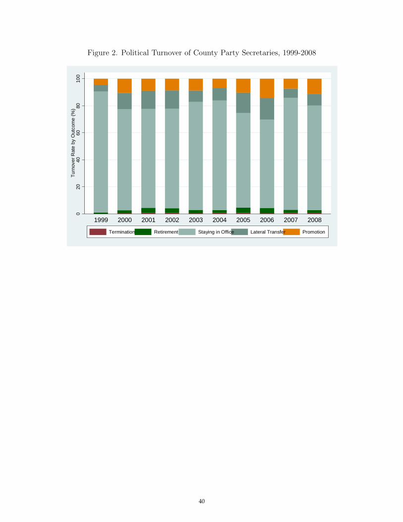
Figure 2. Political Turnover of County Party Secretaries, 1999-2008
36
Figure 2. Political Turnover of County Party Secretaries, 1999-2008
020
4060
8010
0T
urn
over
Rat
e b
y O
utco
me
(%
)
1999 2000 2001 2002 2003 2004 2005 2006 2007 2008
Termination Retirement Staying in Office Lateral Transfer Promotion
40
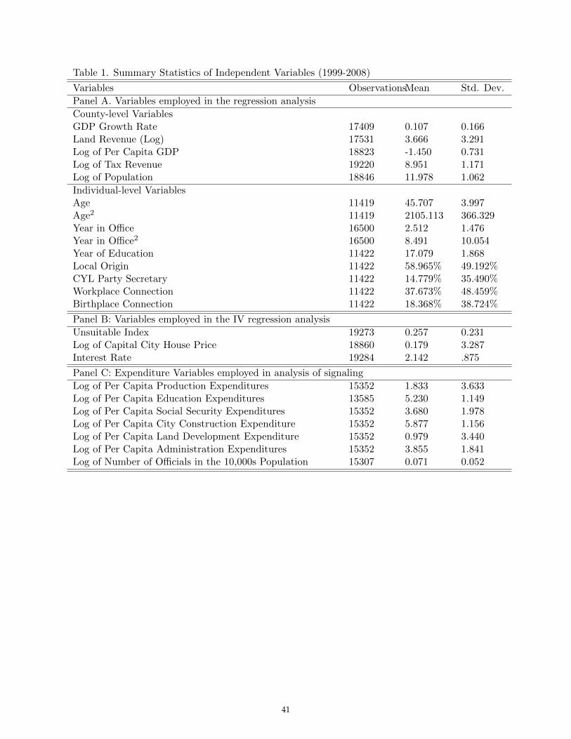
Table 1. Summary Statistics of Independent Variables (1999-2008)
Variables ObservationsMean Std. Dev.
Panel A. Variables employed in the regression analysis
County-level VariablesGDP Growth Rate 17409 0.107 0.166Land Revenue (Log) 17531 3.666 3.291Log of Per Capita GDP 18823 -1.450 0.731Log of Tax Revenue 19220 8.951 1.171Log of Population 18846 11.978 1.062
Individual-level VariablesAge 11419 45.707 3.997Age2 11419 2105.113 366.329Year in Office 16500 2.512 1.476Year in Office2 16500 8.491 10.054Year of Education 11422 17.079 1.868Local Origin 11422 58.965% 49.192%CYL Party Secretary 11422 14.779% 35.490%Workplace Connection 11422 37.673% 48.459%Birthplace Connection 11422 18.368% 38.724%
Panel B: Variables employed in the IV regression analysis
Unsuitable Index 19273 0.257 0.231Log of Capital City House Price 18860 0.179 3.287Interest Rate 19284 2.142 .875
Panel C: Expenditure Variables employed in analysis of signaling
Log of Per Capita Production Expenditures 15352 1.833 3.633Log of Per Capita Education Expenditures 13585 5.230 1.149Log of Per Capita Social Security Expenditures 15352 3.680 1.978Log of Per Capita City Construction Expenditure 15352 5.877 1.156Log of Per Capita Land Development Expenditure 15352 0.979 3.440Log of Per Capita Administration Expenditures 15352 3.855 1.841Log of Number of Officials in the 10,000s Population 15307 0.071 0.052
41

Table 2. Land Revenue Windfall and Political Turnover, Baseline Model
Linear Model Ordered LogitPolitical Turnover (Termination=0; Retirement=1; Same Level=2; Promotion=3)
(1) (2) (3) (4) (5) (6) (7)GDP Growth Rate 0.069*** 0.067*** 0.050 0.071** 0.062** 0.658** 0.643**
(0.026) (0.026) (0.034) (0.035) (0.025) (0.258) (0.254)Land Revenue (Log) 0.006*** 0.007** 0.006*** 0.049*** 0.049***
(0.002) (0.003) (0.002) (0.016) (0.016)GDP GR*Land Rev. -0.039*** -0.333***
(0.012) (0.106)Land Price (Log) 0.015***
(0.003)Area of Land Sale (Log) -0.007
(0.005)Age 0.161*** 0.160*** 0.433*** 0.174*** 0.158*** 1.680*** 1.663***
(0.028) (0.028) (0.058) (0.032) (0.028) (0.309) (0.311)Age2 -0.002*** -0.002*** -0.005*** -0.002*** -0.002*** -0.019*** -0.019***
(0.000) (0.000) (0.001) (0.000) (0.000) (0.003) (0.003)Years of Education 0.010*** 0.010*** 0.012*** 0.010*** 0.098*** 0.096***
(0.003) (0.003) (0.005) (0.003) (0.030) (0.030)Local Origin -0.016 -0.015 -0.018 -0.016 -0.183 -0.195
(0.012) (0.012) (0.017) (0.012) (0.125) (0.125)CYL Party Secretary 0.063*** 0.063*** 0.060*** 0.063*** 0.572*** 0.563***(CYL PS) (0.016) (0.016) (0.023) (0.016) (0.151) (0.151)Workplace Connection 0.081*** 0.080*** 0.064*** 0.079*** 0.807*** 0.794***(WC) (0.013) (0.013) (0.017) (0.013) (0.121) (0.120)Birthplace Connection 0.100*** 0.099*** 0.105*** 0.099*** 0.952*** 0.947***(BC) (0.015) (0.015) (0.021) (0.015) (0.135) (0.135)Cutoff Point 1 41.843*** 41.858***
(8.099) (8.080)Cutoff Point 2 43.633*** 43.655***
(8.117) (8.099)Cutoff Point 3 51.941*** 51.982***
(8.134) (8.117)Control variables† Yes Yes Yes Yes Yes Yes YesCounty-and Year-FEs Yes Yes Yes Yes Yes Yes YesPerson Fixed Effects No No Yes No No No NoClustered at Pref. Yes Yes Yes Yes Yes Yes YesNumber of Observation 10361 10361 10361 5937 10361 10361 10361Adj. R-squared 0.046 0.048 0.121 0.049 0.050 0.216 0.218
†Control variables include per capita GDP (log), population (log), and total tax revenue (log), year in officeand its squared term and tenure length. Robust Standard errors in parentheses; * p<0.10, ** p<0.05, ***p<0.01; Constant terms are not reported
42
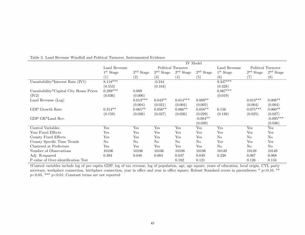
Table 3. Land Revenue Windfall and Political Turnover, Instrumented Evidence
IV ModelLand Revenue Political Turnover Land Revenue Political Turnover1st Stage 2nd Stage 2nd Stage 2nd Stage 2nd Stage 1st Stage 2nd Stage 2nd Stage(1) (2) (3) (4) (5) (6) (7) (8)
Unsuitability*Interest Rate (IV1) 8.118*** -0.244 9.347***(0.553) (0.164) (0.428)
Unsuitability*Capital City House Prices 0.289*** 0.009 0.067***(IV2) (0.036) (0.006) (0.019)Land Revenue (Log) 0.013*** 0.043** 0.014*** 0.009** 0.013*** 0.008**
(0.004) (0.021) (0.004) (0.005) (0.004) (0.004)GDP Growth Rate 0.314** 0.065** 0.056** 0.066** 0.058** 0.156 0.075*** 0.060**
(0.159) (0.026) (0.027) (0.026) (0.029) (0.138) (0.025) (0.027)GDP GR*Land Rev. -0.084** -0.095***
(0.039) (0.036)Control Variables Yes Yes Yes Yes Yes Yes Yes YesYear Fixed Effects Yes Yes Yes Yes Yes Yes Yes YesCounty Fixed Effects Yes Yes Yes Yes Yes No No NoCounty Specific Time Trends No No No No No Yes Yes YesClustered at Prefecture Yes Yes Yes Yes Yes No No NoNumber of Observations 10106 10106 10106 10106 10106 10149 10149 10149Adj. R-squared 0.394 0.048 0.004 0.047 0.049 0.238 0.067 0.068P-value of Over-identification Test 0.182 0.121 0.126 0.134
†Control variables include log of per capita GDP, log of tax revenue, log of population, age, age square, years of education, local origin, CYL partysecretary, workplace connection, birthplace connection, year in office and year in office square; Robust Standard errors in parentheses; * p<0.10, **p<0.05, *** p<0.01; Constant terms are not reported
43

Table 4. The Effect of County Party Secretaries’ Characteristics (Including Factional ties, Workplace Connectionand Birthplace Connection) on Land Unsuitability and House Prices
Land Unsuitability Index Log of Capital City House Price(1) (2) (3) (4) (5) (6) (7) (8) (9) (10)
Age† -0.007 0.004 -0.007 -0.007 -0.007 0.013 0.007 0.013 0.013 0.014(0.009) (0.014) (0.009) (0.009) (0.009) (0.016) (0.010) (0.016) (0.016) (0.016)
Age2 0.000 -0.000 0.000 0.000 0.000 -0.000 -0.000 -0.000 -0.000 -0.000(0.000) (0.000) (0.000) (0.000) (0.000) (0.000) (0.000) (0.000) (0.000) (0.000)
Education -0.001 -0.000 -0.001 -0.001 -0.001 0.001 -0.001 0.001 0.001 0.000(0.001) (0.002) (0.001) (0.001) (0.001) (0.002) (0.001) (0.002) (0.002) (0.002)
CYL PS 0.004 0.004 1.970 0.004 0.004 0.006 -0.001 -3.661 0.006 0.006(0.005) (0.007) (2.918) (0.005) (0.005) (0.008) (0.007) (6.811) (0.009) (0.008)
CYL PS*Year -0.001 0.002(0.001) (0.003)
WC -0.004 -0.005 -0.004 1.319 -0.004 0.004 0.009 0.004 4.628 0.004(0.004) (0.006) (0.004) (2.519) (0.005) (0.007) (0.006) (0.007) (5.699) (0.007)
WC*Year -0.001 -0.002(0.001) (0.003)
BC -0.000 0.003 -0.000 -0.000 -1.673 0.013 0.006 0.013 0.012 23.423**(0.005) (0.009) (0.005) (0.005) (2.878) (0.012) (0.009) (0.012) (0.012) (9.755)
BC*Year 0.001 -0.012**(0.001) (0.005)
Pref.-and Year-FE Yes Yes Yes Yes Yes Yes Yes Yes Yes YesRobust SE Yes Yes Yes Yes Yes Yes Yes Yes Yes YesNo. of Obs. 3849 2213 3849 3849 3849 3530 1913 3530 3530 3530Adj. R-squared 0.751 0.737 0.751 0.751 0.751 0.997 0.920 0.997 0.997 0.997
†Refers to age when the county party secretaries took office. Standard errors in parentheses;* p<0.10, ** p<0.05, *** p<0.01; Constant terms are
not reported.
44

Table 5. The Decomposition of Performance Indicators*
Between WithinPrefecture PrefectureVariance Variance
Per Capita GDP (log) 66.14% 33.86%GDP Growth Rate 99.43% 0.57%Per Capita Total Revenue (log) 60.79% 39.21%Total Revenue Growth Rate 96.94% 3.06%Total Employment Population (log) 68.35% 31.65%Average Salary of Urban Employee (log) 72.90% 27.10%Per Capita Total Fixed Asset Investment (log) 65.81% 34.19%
Extra-budgetary Revenue (log) 32.52% 67.48%Land Revenue (log) 14.73% 85.27%
* The indicators are from the 2008 statistics.
45
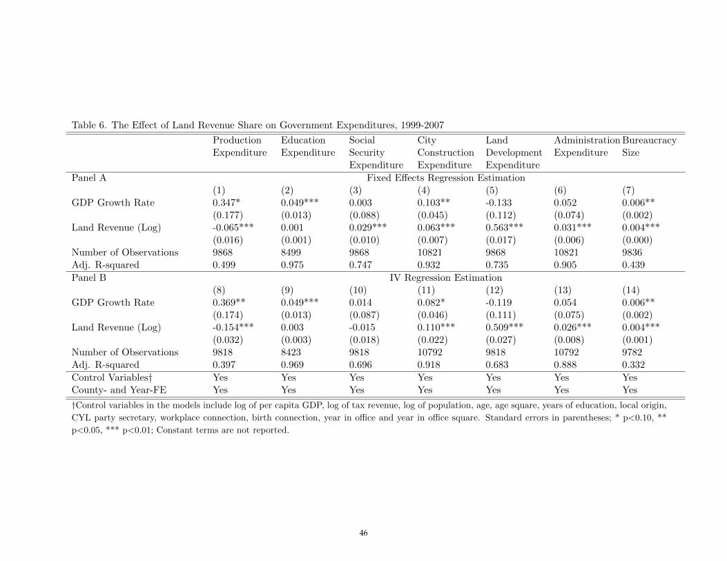
Table 6. The Effect of Land Revenue Share on Government Expenditures, 1999-2007
Production Education Social City Land Administration BureaucracyExpenditure Expenditure Security Construction Development Expenditure Size
Expenditure Expenditure Expenditure
Panel A Fixed Effects Regression Estimation(1) (2) (3) (4) (5) (6) (7)
GDP Growth Rate 0.347* 0.049*** 0.003 0.103** -0.133 0.052 0.006**(0.177) (0.013) (0.088) (0.045) (0.112) (0.074) (0.002)
Land Revenue (Log) -0.065*** 0.001 0.029*** 0.063*** 0.563*** 0.031*** 0.004***(0.016) (0.001) (0.010) (0.007) (0.017) (0.006) (0.000)
Number of Observations 9868 8499 9868 10821 9868 10821 9836Adj. R-squared 0.499 0.975 0.747 0.932 0.735 0.905 0.439
Panel B IV Regression Estimation(8) (9) (10) (11) (12) (13) (14)
GDP Growth Rate 0.369** 0.049*** 0.014 0.082* -0.119 0.054 0.006**(0.174) (0.013) (0.087) (0.046) (0.111) (0.075) (0.002)
Land Revenue (Log) -0.154*** 0.003 -0.015 0.110*** 0.509*** 0.026*** 0.004***(0.032) (0.003) (0.018) (0.022) (0.027) (0.008) (0.001)
Number of Observations 9818 8423 9818 10792 9818 10792 9782Adj. R-squared 0.397 0.969 0.696 0.918 0.683 0.888 0.332
Control Variables† Yes Yes Yes Yes Yes Yes YesCounty- and Year-FE Yes Yes Yes Yes Yes Yes Yes
†Control variables in the models include log of per capita GDP, log of tax revenue, log of population, age, age square, years of education, local origin,
CYL party secretary, workplace connection, birth connection, year in office and year in office square. Standard errors in parentheses; * p<0.10, **
p<0.05, *** p<0.01; Constant terms are not reported.
46

(Continued on the table)
Production Education Social City Land Administration BureaucracyExpenditure Expenditure Security Construction Development Expenditure Size
Expenditure Expenditure Expenditure
Panel C IV Regression Estimation(15) (16) (17) (18) (19) (20) (21)
GDP Growth Rate 0.367** 0.049*** 0.013 0.001 -0.118 0.047 0.006**(0.176) (0.013) (0.087) (0.119) (0.112) (0.076) (0.003)
Land Revenue (Log) -0.082 0.001 -0.003 0.258*** 0.217*** 0.177*** 0.008***(0.079) (0.009) (0.050) (0.081) (0.079) (0.048) (0.002)
Land Revenue*Year in Office -0.057 0.002 -0.012 0.178*** 0.197*** -0.103*** -0.003*(0.058) (0.005) (0.033) (0.050) (0.049) (0.028) (0.002)
Land Revenue*Year in Office2 0.008 -0.000 0.002 -0.021*** -0.023*** 0.013*** 0.000*(0.009) (0.001) (0.005) (0.007) (0.007) (0.004) (0.000)
Number of Observations 9818 8423 9818 9818 9818 10792 9782Adj. R-squared 0.395 0.969 0.696 0.769 0.671 0.885 0.328
Control Variables† Yes Yes Yes Yes Yes Yes YesCounty- and Year-Fixed Effects Yes Yes Yes Yes Yes Yes Yes
†Control variables in the models include log of per capita GDP, log of tax revenue, log of population, age, age square, years of education, local origin,
CYL party secretary, workplace connection, birth connection, year in office and year in office square. Standard errors in parentheses; * p<0.10, **
p<0.05, *** p<0.01; Constant terms are not reported.
47

Table 7. Heterogeneous Effects of Land Revenue on Political Turnover, 1999-2008
IV Estimation on Political Turnover(1) (2) (3) (4) (5)
Land Revenue (Log) 0.015*** 0.006 0.009** -0.000 0.011***(0.004) (0.005) (0.004) (0.006) (0.004)
CYL Party Secretary 0.068 0.061*** 0.064*** 0.066*** 0.063***(0.050) (0.050) (0.016) (0.017) (0.016)
CYL Party Secretary*Land Revenue -0.001(0.012)
Workplace Connection 0.080*** 0.003 0.079*** 0.078*** 0.071***(0.013) (0.040) (0.013) (0.013) (0.012)
Workplace Connection*Land Revenue 0.019**(0.009)
Birthplace Connection 0.098*** 0.097*** -0.027 0.097*** 0.101***(0.018) (0.018) (0.065) (0.018) (0.017)
Birthplace Connection*Land Revenue 0.032**(0.016)
Above Age -0.594**(0.300)
Above Age*Land Revenue 0.071**(0.034)
Education 0.010*** 0.009*** 0.011*** 0.010*** 0.011***(0.003) (0.003) (0.003) (0.003) (0.003)
Education*Land Revenue 0.001(0.003)
Control Variables † Yes Yes Yes Yes YesCounty-and Year-Fixed Effects Yes Yes Yes Yes YesClustered at Prefecture Yes Yes Yes Yes YesNumber of Observations 10106 10106 10106 10406 10406Adj. R-squared 0.130 0.135 0.137 0.169 0.134P-value of Over-identification Test 0.295 0.284 0.059 0.292 0.174
†Control variables in the models include log of per capita GDP, log of tax revenue, log of population, age,
age square, local origin, year in office and year in office square. Robust standard errors in parentheses; *
p<0.10, ** p<0.05, *** p<0.01; Constant terms are not reported.
48

Table 8 The Effects of Land Revenue on Political Turnover and Expenditures during Crackdownon Corruption, 1999-2008
2SLS Estimation on: Province Prefecture Province PrefecturePolitical Turnover
(1) (2) (3) (4)Land Revenue (Log) 0.023*** 0.023*** 0.014*** 0.018***
(0.007) (0.007) (0.004) (0.005)Corruption Crackdown 0.076** 0.077**
(0.037) (0.034)Land Revenue*Corruption Crackdown -0.017* -0.016**
(0.009) (0.008)Number of Corruption Crackdown 0.013** 0.005
(0.006) (0.007)Land Revenue*Number of Corruption Crackdown -0.009** -0.013**
(0.004) (0.005)Number of Observations 10106 10106 10106 10106Adj. R-squared 0.141 0.139 0.144 0.144P-value of Over-identification Test 0.510 0.282 0.338 0.404
City Construction Expenditure(5) (6) (7) (8)
Land Revenue (Log) 0.520*** 0.518*** 0.524*** 0.524***(0.035) (0.039) (0.028) (0.029)
Corruption Crackdown -0.068 -0.009(0.241) (0.220)
Land Revenue*Corruption Crackdown 0.019 0.021(0.055) (0.050)
Number of Corruption Crackdown 0.01 0.002(0.034) (0.030)
Land Revenue*Number of Corruption Crackdown -0.006 0.006(0.025) (0.025)
Number of Observations 9818 9818 9818 9818Adj. R-squared 0.775 0.775 0.775 0.775
Bureaucracy Size(9) (10) (11) (12)
Land Revenue (Log) 0.005*** 0.005*** 0.004*** 0.004***(0.001) (0.001) (0.001) (0.001)
Corruption Crackdown 0.012*** 0.007(0.005) (0.005)
Land Revenue*Corruption Crackdown -0.003** -0.002(0.001) (0.001)
Number of Corruption Crackdown 0.001 0.001*(0.001) 0.000
Land Revenue*Number of Corruption Crackdown 0.000 -0.001***(0.001) 0.000
Number of Observations 9782 9782 9782 9782Adj. R-squared 0.328 0.329 0.33 0.332Control Variables † yes yes yes yesCounty-and Year-Fixed Effects yes yes yes yesClustered at Prefecture yes yes yes yes
†Control variables in the models include log of per capita GDP, log of tax revenue, log of population, age,age square, years of education, local origin, CYL party secretary, workplace connection, birth connection,year in office and year in office square. Robust standard errors in parentheses; * p<0.10, ** p<0.05, ***p<0.01; Constant terms are not reported.
49
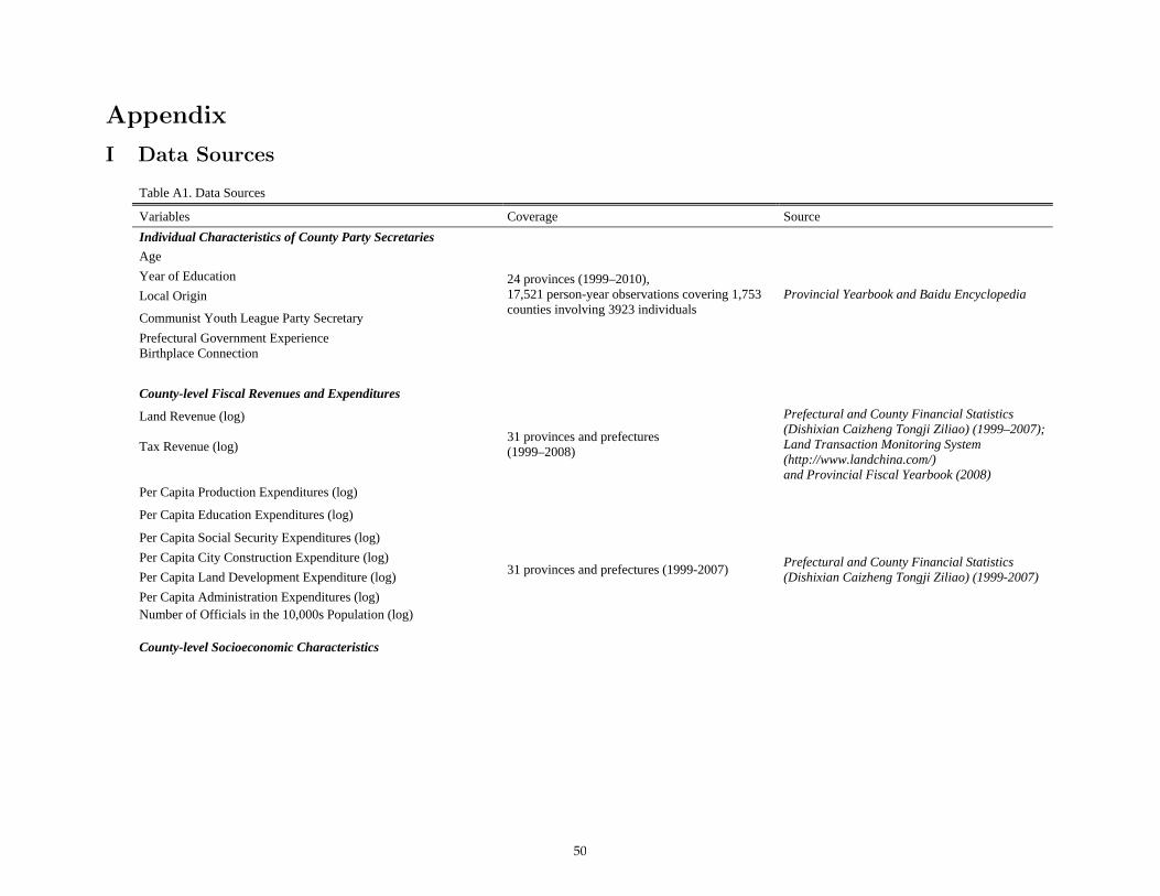
Appendix
I Data Sources
46
APPENDIX A. Data Sources
Table A1. Data Sources
Variables Coverage Source
Individual Characteristics of County Party Secretaries
24 provinces (1999–2010), 17,521 person-year observations covering 1,753 counties involving 3923 individuals
Provincial Yearbook and Baidu Encyclopedia
Age
Year of Education
Local Origin
Communist Youth League Party Secretary
Prefectural Government Experience Birthplace Connection
County-level Fiscal Revenues and Expenditures
Land Revenue (log)
31 provinces and prefectures (1999–2008)
Prefectural and County Financial Statistics (Dishixian Caizheng Tongji Ziliao) (1999–2007); Land Transaction Monitoring System (http://www.landchina.com/) and Provincial Fiscal Yearbook (2008)
Tax Revenue (log)
Per Capita Production Expenditures (log)
Per Capita Education Expenditures (log)
31 provinces and prefectures (1999-2007) Prefectural and County Financial Statistics (Dishixian Caizheng Tongji Ziliao) (1999-2007)
Per Capita Social Security Expenditures (log)
Per Capita City Construction Expenditure (log)
Per Capita Land Development Expenditure (log)
Per Capita Administration Expenditures (log) Number of Officials in the 10,000s Population (log) County-level Socioeconomic Characteristics
50

47
GDP Growth Rate 31 provinces and prefectures (1999–2008)
Statistical Yearbook of Regional Economies (Quyu Jingji Tongji Nianjian) (2002–2009), county level data and Provincial Statistical Yearbook (Sheng Tongji Nianjian) (1999–2001)
Per Capita GDP (log) Population (log) GIS Data & Land Related Data
Slope Map 31 provinces and prefectures SGS Digital Elevation Model (DEM) at 90 square-meter-cell grid resolution
County Administrative Boundary Maps 31 provinces and prefectures China County Population Census Data with GIS Maps (1953, 1964, 1982, 1990, 2000) from the China Data Center
Interest Rate Capital City House Price
10 years (1999-2008) 31 provinces and prefectures (1999-2008)
The website of the People’s Bank of China (http://www.pbc.gov.cn/) Statistical Yearbook of Regional Economies (Quyu Jingji Tongji Nianjian) (2000–2009), prefectural level data
Corruption Case 10 years (1999-2008) 524 cases
Procuratorial Daily (Jiangcha Ribao)
51

II Definitions of, and Criteria Employed in, Coding Political Turnover
There are altogether four political turnover outcomes: Promotion, Lateral Transfer, Re-
tirement, and Termination. Table A2 below provides the Criteria Employed in Coding
Political Turnover.
i Promotion
Typically, county party secretaries would be promoted to the position of vice party secre-
tary or mayor at the prefecture level. In addition, following the Chinese Communist Party’s
own internal ranking system, appointment to head one of the several “strategically impor-
tant” departments (prominent examples include the Department of Organization (Zuzhi Bu)
and Public Security Bureau) is considered equivalent in rank to either vice party secretary
or mayor at the prefecture level and thus promotion. For details see “Provisional Terms
and Regulations Governing the Top Leadership (Party and Government Officials)” (Guojia
Gongwuyuan Zhanxing Tiaoli), State Council, and “Regulations on the Selection and Ap-
pointment of Top Party Secretaries and Government Officials” (Dangzheng Lingdao Ganbu
Xuanba Renyong Gongzuo Tiaoli), Department of Organization. See also Li (2001).
ii Lateral Transfer or Staying in Office
Lateral transfer refers to appointments to positions at essentially the same rank. For
example, this could conceivably occur where a county chief is transferred from one county
to another either in the same capacity as county party secretary or as head of what the
Chinese regards as a “non-strategic” department at the prefecture level (examples of such
departments include the Department of Education or Workplace Safety). We consider such
transfers as “lateral” because both the ranking and compensation that come with the new
appointment are the same as those associated with the previous one, so they are clearly not
promotions.
Staying in office refers to the situation where a county party secretary stays in the same
52

position for one more year. Given the ranking will not change if the party secretary stays in
office, it is equivalent to a lateral transfer.
iii Retirement
Upon retirement one may be appointed to take up an advisory position in the Chinese
People’s Political Consultation Committee (Zhongguo Renmin Zhengzhi Xieshang Huiyi) or
the People’s Congress.
iv Termination
Termination happened when county party secretary unusually leaves office due to the
incidence of natural death, severe illness, or imprisonment due to wrongdoing.
53

Table A2 Criteria Employed in Coding Political Turnover †
A county party secretary is “promoted” if he/she attains one of the following positions upon the end of term: Deputy Secretary of Prefectural Party Committee (Dijishi Shiwei Fushuji)
Minister of Party Committee Organization Department (Dijishi Shiwei Zuzhibu Buzhang) Minister of Party Committee Propaganda Department (Dijishi Shiwei Xuanchuanbu Buzhang)
Secretary of the Discipline Inspection Commission (Dijishi Jiwei Shuji) Vice Mayor (Dijishi Fu Shizhang)
Secretary General (Dijishi Shizhengfu Mishuzhang) Chief of Public Security Bureau (Dijishi Gonganju Juzhang)
Chief Justice of Intermediate People's Court (Dijishi Zhongji Renminfayuan Yuanzhang)
Chief Procurator of Intermediate People's Procuratorate (Dijishi Zhongji Renminjianchayuan Yuanzhang)
A county party secretary is “transferred laterally” if he/she ends up with one of the following positions upon the end of term:
County Party Secretary (Xianwei Shuji) County City Party Secretary (Xianjishi Shiwei Shuji)
District Party Secretary (Quwei Shuji)
Minister of Party Committee United Front Department (Dijishi Shiwei Tongzhanbu Fubuzhang)
Vice Minister of Party Committee Organization Department (Dijishi Shiwei Zuzhibu Fubuzhang)
Vice Minister of Party Committee Propaganda Department (Dijishi Shiwei Xuanchuanbu Fubuzhang)
Vice Secretary of the Discipline Inspection Commission (Dijishi Jiwei Fushuji)
54

Assistant Mayor (Shizhengfu Shizhang Zhuli) Prefectural Government Counselor (Shizhengfu Xunshiyuan)
Vice Secretary-General (Dijishi Zhengfu Fumishuzhang) Deputy Chief of Public Security Bureau (Dijishi Gonganju Fujuzhang)
Deputy Chief Justice of Intermediate People's Court (Dijishi Zhongji Renminfayuan Fuyuanzhang)
Deputy Chief Procurator of Intermediate People's Procuratorate (Dijishi Zhongji Renminjianchayuan Fuyuanzhang)
Department Head of Prefectural Functional Bureau (e.g. Head of Education Bureau) (Juzhang)
A county party secretary is “retired” if he/she ends up with one of the following positions upon the end of term:
Chairman and Vice-Chairman of the Standing Committee of the People's Congress (Dijishi Shirenda Changweihui Fu/Zhuren)
Chairman and Vice-Chairman of the People's Political Consultative Conference (Dijishi Zhengxie Fu/Zhuxi)
Chairman of Prefectural Trade Union (Dijishi Shizhonggonghui Zhuxi) Chairman of Prefectural Women's Federation (Dijishi Fulian Zhuxi)
† The coding of Political Turnover is based on the administrative rank of the positions to which the county party secretary was subsequently appointed.
55

III Other Supporting Figures and Table
Figure A1. A County Party Secretary’s Vita in Baidu Encyclopedia
C F
C. Other Suppo
Figure A1. A County
Note: This eThe curricu
rting Figures &
y Party Secretary’s
example serves to iulum vitae in turn ar
& Tables
Vita in Baidu Ency
illustrate how the core obtained from th
yclopedia
ounty party secretare pertinent Chinese
52
ries’ dataset is conste government websi
tructed based upon ites.
their curriculum vit
tae in Baidu Encycllopedia.
56

Figure A2. The Distribution of Tenure Duration of County Party Secretaries, 1999-2008.
53
Figure A2. The Distribution of Tenure Duration of County Party Secretaries, 1999-2008.
050
010
0015
00
Nu
mbe
r of
CP
S
1 2 3 4 5 6 7 8 9 10 11 12Tenure Duration
57
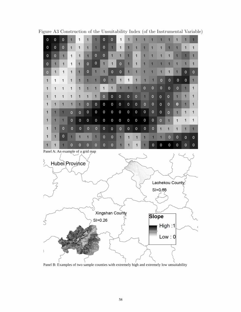
Figure A3 Construction of the Unsuitability Index (of the Instrumental Variable)
Figu
Pane
Pane
ure A3 Constru
el A: An exam
el B: Example
uction of the U
mple of a grid m
es of two samp
Unsuitability I
map
ple counties w
54
Index (of the I
with extremely
Instrumental V
y high and extr
Variable)
remely low unnsuitability
58

Table A3. Land Revenue and GDP Growth
GDP Growth RateFE FE FE IV(1) (2) (3) (4)
Unsuitability*Interest Rate (IV1) 0.018(0.012)
Unsuitability*Capital City House Prices (IV2) 0.005(0.003)
Land Revenue (Log) 0.002*** 0.003(0.001) (0.002)
Control Variables Yes Yes Yes YesCounty.-and Year-Fixed Effects Yes Yes Yes YesClustered at Prefecture Yes Yes Yes YesNumber of Observations 10821 10593 10821 10555Adj. R-squared 0.162 0.163 0.163 0.014P-value of Over-identification Test 0.163
†Controls include per capita GDP (log), population (log), and total tax revenue (log), age and its squared
term, year of education, local origin, CYL party secretary, workplace connection, birthplace connection,
year in office and its squared term and tenure length. Robust Standard errors in parentheses; * p<0.10, **
p<0.05, *** p<0.01; Constant terms are not reported.
59
Top Related