


Languages
Pages
Legal


Polynomial Approximation: Practical ComputationsPolynomial Approximation, Higher Order Matching
Beyond Hermite Interpolatory Polynomials
Numerical Analysis and ComputingLecture Notes #5 — Interpolation and Polynomial
ApproximationDivided Differences, and Hermite Interpolatory Polynomials
Joe Mahaffy,〈[email protected]〉
Department of MathematicsDynamical Systems Group
Computational Sciences Research Center
San Diego State UniversitySan Diego, CA 92182-7720
http://www-rohan.sdsu.edu/∼jmahaffy
Spring 2010
Joe Mahaffy, 〈[email protected]〉 #5 Interpolation and Polynomial Approximation — (1/41)

Polynomial Approximation: Practical ComputationsPolynomial Approximation, Higher Order Matching
Beyond Hermite Interpolatory Polynomials
Outline
1 Polynomial Approximation: Practical ComputationsRepresenting PolynomialsDivided DifferencesDifferent forms of Divided Difference Formulas
2 Polynomial Approximation, Higher Order MatchingOsculating PolynomialsHermite Interpolatory PolynomialsComputing Hermite Interpolatory Polynomials
3 Beyond Hermite Interpolatory Polynomials
Joe Mahaffy, 〈[email protected]〉 #5 Interpolation and Polynomial Approximation — (2/41)

Polynomial Approximation: Practical ComputationsPolynomial Approximation, Higher Order Matching
Beyond Hermite Interpolatory Polynomials
Recap and Lookahead
Previously:Neville’s Method to successively generate higher degree polynomial ap-proximations at a specific point. — If we need to compute the polyno-mial at many points, we have to re-run Neville’s method for each point.O(n2) operations/point.
Algorithm: Neville’s Method
To evaluate the polynomial that interpolates the n + 1 points (xi , f (xi )), i = 0, . . . , n
at the point x :
1. Initialize Qi,0 = f (xi ).2. FOR i = 1 : n
FOR j = 1 : i
Qi,j =(x − xi−j )Qi,j−1 − (x − xi )Qi−1,j−1
xi − xi−j
END
END
3. Output the Q-table.
Joe Mahaffy, 〈[email protected]〉 #5 Interpolation and Polynomial Approximation — (3/41)

Polynomial Approximation: Practical ComputationsPolynomial Approximation, Higher Order Matching
Beyond Hermite Interpolatory Polynomials
Recap and Lookahead
Next:Use divided differences to generate the polynomials∗ themselves.∗ The coefficients of the polynomials. Once we have those, we can
quickly (remember Horner’s method?) compute the polynomial inany desired points. O(n) operations/point.
Algorithm: Horner’s Method
Input: Degree n; coefficients a0, a1, . . . , an; x0
Output: y = P(x0), z = P′(x0).
1. Set y = an, z = an
2. For j = (n − 1), (n − 2), . . . , 1
Set y = x0y + aj , z = x0z + y
3. Set y = x0y + a0
4. Output (y , z)
5. End program
Joe Mahaffy, 〈[email protected]〉 #5 Interpolation and Polynomial Approximation — (4/41)

Polynomial Approximation: Practical ComputationsPolynomial Approximation, Higher Order Matching
Beyond Hermite Interpolatory Polynomials
Representing PolynomialsDivided DifferencesDifferent forms of Divided Difference Formulas
Representing Polynomials
If Pn(x) is the nth degree polynomial that agrees with f (x) at thepoints {x0, x1, . . . , xn}, then we can (for the appropriate constants{a0, a1, . . . , an}) write:
Pn(x) = a0 + a1(x − x0) + a2(x − x0)(x − x1) + · · ·· · · + an(x − x0)(x − x1) · · · (x − xn−1)
Joe Mahaffy, 〈[email protected]〉 #5 Interpolation and Polynomial Approximation — (5/41)
Polynomial Approximation: Practical ComputationsPolynomial Approximation, Higher Order Matching
Beyond Hermite Interpolatory Polynomials
Representing PolynomialsDivided DifferencesDifferent forms of Divided Difference Formulas
Representing Polynomials
If Pn(x) is the nth degree polynomial that agrees with f (x) at thepoints {x0, x1, . . . , xn}, then we can (for the appropriate constants{a0, a1, . . . , an}) write:
Pn(x) = a0 + a1(x − x0) + a2(x − x0)(x − x1) + · · ·· · · + an(x − x0)(x − x1) · · · (x − xn−1)
Note that we can evaluate this “Horner-style,” by writing
Pn(x) = a0 + (x − x0) (a1 + (x − x1) (a2+ · · ·· · · + (x − xn−2) (an−1 + an(x − xn−1)))) ,
so that each step in the Horner-evaluation consists of asubtraction, a multiplication, and an addition.
Joe Mahaffy, 〈[email protected]〉 #5 Interpolation and Polynomial Approximation — (5/41)

Polynomial Approximation: Practical ComputationsPolynomial Approximation, Higher Order Matching
Beyond Hermite Interpolatory Polynomials
Representing PolynomialsDivided DifferencesDifferent forms of Divided Difference Formulas
Finding the Constants {a0, a1, . . . , an} “Just Algebra”
Given the relation
Pn(x) = a0 + a1(x − x0) + a2(x − x0)(x − x1) + · · ·· · · + an(x − x0)(x − x1) · · · (x − xn−1)
at x0: a0 = Pn(x0) = f (x0).
at x1: f (x0) + a1(x1 − x0) = Pn(x1) = f (x1)
⇒ a1 =f (x1) − f (x0)
x1 − x0.
at x2: a2 =f (x2) − f (x0)
(x2 − x0)(x2 − x1)−
f (x1) − f (x0)
(x2 − x0)(x1 − x0).
This gets massively ugly fast! — We need some nice cleannotation!
Joe Mahaffy, 〈[email protected]〉 #5 Interpolation and Polynomial Approximation — (6/41)

Polynomial Approximation: Practical ComputationsPolynomial Approximation, Higher Order Matching
Beyond Hermite Interpolatory Polynomials
Representing PolynomialsDivided DifferencesDifferent forms of Divided Difference Formulas
Sir Isaac Newton to the Rescue: Divided Differences
Zeroth Divided Difference:
f [xi ] = f (xi ).
First Divided Difference:
f [xi , xi+1] =f [xi+1] − f [xi ]
xi+1 − xi
.
Second Divided Difference:
f [xi , xi+1, xi+2] =f [xi+1, xi+2] − f [xi , xi+1]
xi+2 − xi
.
kth Divided Difference:
f [xi , xi+1, . . . , xi+k ] =f [xi+1, xi+2, . . . , xi+k ] − f [xi , xi+1, . . . , xi+k−1]
xi+k − xi
.
Joe Mahaffy, 〈[email protected]〉 #5 Interpolation and Polynomial Approximation — (7/41)

Polynomial Approximation: Practical ComputationsPolynomial Approximation, Higher Order Matching
Beyond Hermite Interpolatory Polynomials
Representing PolynomialsDivided DifferencesDifferent forms of Divided Difference Formulas
The Constants {a0, a1, . . . , an} — Revisited
We had
at x0: a0 = Pn(x0) = f (x0).
at x1: f (x0) + a1(x1 − x0) = Pn(x1) = f (x1)
⇒ a1 =f (x1) − f (x0)
x1 − x0.
at x2: a2 =f (x2) − f (x0)
(x2 − x0)(x2 − x1)−
f (x1) − f (x0)
(x2 − x0)(x1 − x0).
Clearly:a0 = f [x0], a1 = f [x0, x1].
We may suspect that a2 = f [x0, x1, x2], that is indeed so (a “littlebit” of careful algebra will show it), and in general
ak = f[x0, x1, . . . , xk].
Joe Mahaffy, 〈[email protected]〉 #5 Interpolation and Polynomial Approximation — (8/41)

Polynomial Approximation: Practical ComputationsPolynomial Approximation, Higher Order Matching
Beyond Hermite Interpolatory Polynomials
Representing PolynomialsDivided DifferencesDifferent forms of Divided Difference Formulas
Algebra: Chasing down a2 = f [x0, x1, x2]
a2 =f (x2) − f (x0)
(x2 − x0)(x2 − x1)−
f (x1) − f (x0)
(x2 − x1)(x1 − x0)
=(f (x2) − f (x0))(x1 − x0) − (f (x1) − f (x0))(x2 − x0)
(x2 − x0)(x2 − x1)(x1 − x0)
=(x1 − x0)f (x2) − (x2 − x0)f (x1) + (x2 − x0 − x1 + x0)f (x0)
(x2 − x0)(x2 − x1)(x1 − x0)
=(x1 − x0)f (x2) − (x1 − x0 + x2 − x1)f (x1) + (x2 − x1)f (x0)
(x2 − x0)(x2 − x1)(x1 − x0)
=(x1 − x0)(f (x2) − f (x1)) − (x2 − x1)(f (x1) − f (x0))
(x2 − x0)(x2 − x1)(x1 − x0)
=(f (x2) − f (x1))
(x2 − x0)(x2 − x1)−
(f (x1) − f (x0))
(x2 − x0)(x1 − x0)
=f [x1, x2]
x2 − x0−
f [x0, x1]
x2 − x0= f[x0, x1, x2] (!!!)
Joe Mahaffy, 〈[email protected]〉 #5 Interpolation and Polynomial Approximation — (9/41)
Polynomial Approximation: Practical ComputationsPolynomial Approximation, Higher Order Matching
Beyond Hermite Interpolatory Polynomials
Representing PolynomialsDivided DifferencesDifferent forms of Divided Difference Formulas
Newton’s Interpolatory Divided Difference Formula
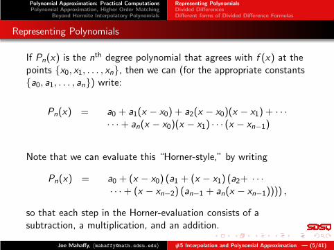
Hence, we can write
Pn(x) = f [x0] +n
∑
k=1
[
f [x0, . . . , xk ]k−1∏
m=0
(x − xm)
]
.
Pn(x) = f [x0] +f [x0, x1](x − x0) +f [x0, x1, x2](x − x0)(x − x1) +f [x0, x1, x2, x3](x − x0)(x − x1)(x − x2) + · · ·
This expression is known as Newton’s Interpolatory DividedDifference Formula.
Joe Mahaffy, 〈[email protected]〉 #5 Interpolation and Polynomial Approximation — (10/41)

Polynomial Approximation: Practical ComputationsPolynomial Approximation, Higher Order Matching
Beyond Hermite Interpolatory Polynomials
Representing PolynomialsDivided DifferencesDifferent forms of Divided Difference Formulas
Computing the Divided Differences (by table)
x f(x) 1st Div. Diff. 2nd Div. Diff.x0 f [x0]
f [x0, x1] =f [x1]−f [x0]
x1−x0
x1 f [x1] f [x0, x1, x2] =f [x1,x2]−f [x0,x1]
x2−x0
f [x1, x2] =f [x2]−f [x1]
x2−x1
x2 f [x2] f [x1, x2, x3] =f [x2,x3]−f [x1,x2]
x3−x1
f [x2, x3] =f [x3]−f [x2]
x3−x2
x3 f [x3] f [x2, x3, x4] =f [x3,x4]−f [x2,x3]
x4−x2
f [x3, x4] =f [x4]−f [x3]
x4−x3
x4 f [x4] f [x3, x4, x5] =f [x4,x5]−f [x3,x4]
x5−x3
f [x4, x5] =f [x5]−f [x4]
x5−x4
x5 f [x5]
Note: The table can be extended with three 3rd divideddifferences, two 4th divided differences, and one 5th divideddifference.
Joe Mahaffy, 〈[email protected]〉 #5 Interpolation and Polynomial Approximation — (11/41)
Polynomial Approximation: Practical ComputationsPolynomial Approximation, Higher Order Matching
Beyond Hermite Interpolatory Polynomials
Representing PolynomialsDivided DifferencesDifferent forms of Divided Difference Formulas
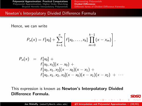
Algorithm: Computing the Divided Differences
Algorithm: Newton’s Divided Differences
Given the points (xi , f (xi )), i = 0, . . . , n.
Step 1: Initialize Fi ,0 = f (xi ), i = 0, . . . , n
Step 2:
FOR i = 1 : n
FOR j = 1 : i
Fi ,j =Fi ,j−1 − Fi−1,j−1
xi − xi−j
END
END
Result: The diagonal, Fi ,i now contains f [x0, . . . , xi ].
Joe Mahaffy, 〈[email protected]〉 #5 Interpolation and Polynomial Approximation — (12/41)

Polynomial Approximation: Practical ComputationsPolynomial Approximation, Higher Order Matching
Beyond Hermite Interpolatory Polynomials
Representing PolynomialsDivided DifferencesDifferent forms of Divided Difference Formulas
A Theoretical Result: Generalization of the Mean Value Theorem
Theorem (Generalized Mean Value Theorem)
Suppose that f ∈ Cn[a, b] and {x0, . . . , xn} are distinct number in[a, b]. Then ∃ ξ ∈ (a, b) :
f [x0, . . . , xn] =f (n)(ξ)
n!.
For n = 1 this is exactly the Mean Value Theorem...
So we have extended to MVT to higher order derivatives!
What is the theorem telling us?
— Newton’s nth divided difference is in some sense an approxi-mation to the nth derivative of f .
Joe Mahaffy, 〈[email protected]〉 #5 Interpolation and Polynomial Approximation — (13/41)

Polynomial Approximation: Practical ComputationsPolynomial Approximation, Higher Order Matching
Beyond Hermite Interpolatory Polynomials
Representing PolynomialsDivided DifferencesDifferent forms of Divided Difference Formulas
Newton vs. Taylor...
Using Newton’s Divided Differences...
PNn (x) = f [x0] + f [x0, x1](x − x0) +
f [x0, x1, x2](x − x0)(x − x1) +f [x0, x1, x2, x3](x − x0)(x − x1)(x − x2) + · · ·
Using Taylor expansion
PTn (x) = f (x0) + f ′(x0)(x − x0) +
12! f ′′(x0)(x − x0)
2 +13! f ′′′(x0)(x − x0)
3 + · · ·
It makes sense that the divided differences are approximating thederivatives in some sense!
Joe Mahaffy, 〈[email protected]〉 #5 Interpolation and Polynomial Approximation — (14/41)
Polynomial Approximation: Practical ComputationsPolynomial Approximation, Higher Order Matching
Beyond Hermite Interpolatory Polynomials
Representing PolynomialsDivided DifferencesDifferent forms of Divided Difference Formulas
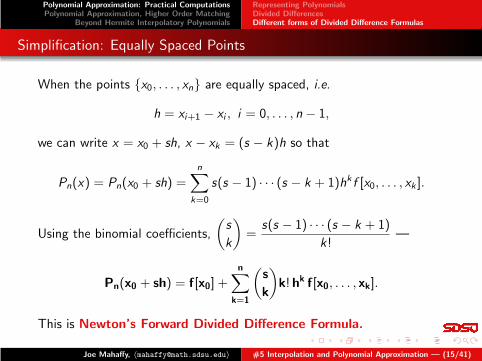
Simplification: Equally Spaced Points
When the points {x0, . . . , xn} are equally spaced, i.e.
h = xi+1 − xi , i = 0, . . . , n − 1,
we can write x = x0 + sh, x − xk = (s − k)h so that
Pn(x) = Pn(x0 + sh) =
n∑
k=0
s(s − 1) · · · (s − k + 1)hk f [x0, . . . , xk ].
Using the binomial coefficients,
(
s
k
)
=s(s − 1) · · · (s − k + 1)
k!—
Pn(x0 + sh) = f[x0] +n
∑
k=1
(
s
k
)
k!hk f[x0, . . . , xk].
This is Newton’s Forward Divided Difference Formula.
Joe Mahaffy, 〈[email protected]〉 #5 Interpolation and Polynomial Approximation — (15/41)
Polynomial Approximation: Practical ComputationsPolynomial Approximation, Higher Order Matching
Beyond Hermite Interpolatory Polynomials
Representing PolynomialsDivided DifferencesDifferent forms of Divided Difference Formulas
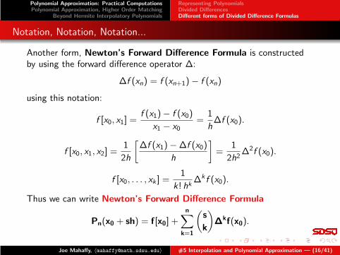
Notation, Notation, Notation...
Another form, Newton’s Forward Difference Formula is constructedby using the forward difference operator ∆:
∆f (xn) = f (xn+1) − f (xn)
using this notation:
f [x0, x1] =f (x1) − f (x0)
x1 − x0=
1
h∆f (x0).
f [x0, x1, x2] =1
2h
[
∆f (x1) − ∆f (x0)
h
]
=1
2h2∆2f (x0).
f [x0, . . . , xk ] =1
k! hk∆k f (x0).
Thus we can write Newton’s Forward Difference Formula
Pn(x0 + sh) = f[x0] +
n∑
k=1
(
s
k
)
∆kf(x0).
Joe Mahaffy, 〈[email protected]〉 #5 Interpolation and Polynomial Approximation — (16/41)

Polynomial Approximation: Practical ComputationsPolynomial Approximation, Higher Order Matching
Beyond Hermite Interpolatory Polynomials
Representing PolynomialsDivided DifferencesDifferent forms of Divided Difference Formulas
Notation, Notation, Notation... Backward Formulas
If we reorder {x0, x1, . . . , xn} → {xn, . . . , x1, x0}, and define the backwarddifference operator ∇:
∇f (xn) = f (xn) − f (xn−1),
we can define the backward divided differences:
f [xn, . . . , xn−k ] =1
k! hk∇k f (xn).
We write down Newton’s Backward Difference Formula
Pn(x) = f[xn] +
n∑
k=1
(−1)k(
−s
k
)
∇kf(xn),
where(
−s
k
)
= (−1)ks(s + 1) · · · (s + k − 1)
k!.
Joe Mahaffy, 〈[email protected]〉 #5 Interpolation and Polynomial Approximation — (17/41)

Polynomial Approximation: Practical ComputationsPolynomial Approximation, Higher Order Matching
Beyond Hermite Interpolatory Polynomials
Representing PolynomialsDivided DifferencesDifferent forms of Divided Difference Formulas
Forward? Backward? I’m Confused!!!
x f (x) 1st Div. Diff. 2nd Div. Diff.x0 f [x0]
f[x0, x1] =f[x1]−f[x0]
x1−x0
x1 f [x1] f[x0, x1, x2] =f[x1,x2]−f[x0,x1]
x2−x0
f [x1, x2] =f [x2]−f [x1]
x2−x1
x2 f [x2] f [x1, x2, x3] =f [x2,x3]−f [x1,x2]
x3−x1
f [x2, x3] =f [x3]−f [x2]
x3−x2
x3 f [x3] f [x2, x3, x4] =f [x3,x4]−f [x2,x3]
x4−x2
f [x3, x4] =f [x4]−f [x3]
x4−x3
x4 f [x4] f[x3, x4, x5] =f[x4,x5]−f[x3,x4]
x5−x3
f[x4, x5] =f[x5]−f[x4]
x5−x4
x5 f [x5]
Forward: The fwd div. diff. are the top entries in the table.
Backward: The bwd div. diff. are the bottom entries in the table.
Joe Mahaffy, 〈[email protected]〉 #5 Interpolation and Polynomial Approximation — (18/41)

Polynomial Approximation: Practical ComputationsPolynomial Approximation, Higher Order Matching
Beyond Hermite Interpolatory Polynomials
Representing PolynomialsDivided DifferencesDifferent forms of Divided Difference Formulas
Forward? Backward? — Straight Down the Center!
The Newton formulas works best for points close to the edge ofthe table; if we want to approximate f (x) close to the center, wehave to work some more...
x f (x) 1st Div. Diff. 2nd Div. Diff. 3rd Div. Diff. 4th Div. Diff.x−2 f [x
−2]f [x
−2, x−1]
x−1 f [x
−1] f [x−2, x
−1, x0]f[x
−1, x0] f[x−2, x
−1, x0, x1]x0 f[x0] f[x
−1, x0, x1] f[x−2, x
−1, x0, x1, x2]f[x0, x1] f[x
−1, x0, x1, x2]x1 f [x1] f [x0, x1, x2] f [x
−1, x0, x1, x2, x3]f [x1, x2] f [x0, x1, x2, x3]
x2 f [x2] f [x1, x2, x3]f [x2, x3]
x3 f [x3]
We are going to construct Stirling’s Formula — a scheme usingcentered differences. In particular we are going to use the blue(centered at x0) entries, and averages of the red (straddling the x0
point) entries.
Joe Mahaffy, 〈[email protected]〉 #5 Interpolation and Polynomial Approximation — (19/41)

Polynomial Approximation: Practical ComputationsPolynomial Approximation, Higher Order Matching
Beyond Hermite Interpolatory Polynomials
Representing PolynomialsDivided DifferencesDifferent forms of Divided Difference Formulas
Stirling’s Formula — Approximating at Interior Points
Assume we are trying to approximate f (x) close to the interiorpoint x0:
Pn(x) = P2m+1(x) = f [x0] + shf [x−1, x0] + f [x0, x1]
2+ s2h2 f [x−1, x0, x1]
+ s(s2 − 1)h3 f [x−2, x−1, x0, x1] + f [x−1, x0, x1, x2]
2+ s2(s2 − 1)h4 f [x−2, x−1, x0, x1, x2]
+ . . .
+ s2(s2 − 1) · · · (s2 − (m − 1)2)h2m f [x−m, . . . , xm]
+ s(s2 − 1) · · · (s2 − m2)h2m+1
·f [x−m−1, . . . , xm] + f [x−m, . . . , xm+1]
2
If n = 2m + 1 is odd, otherwise delete the last two lines.
Joe Mahaffy, 〈[email protected]〉 #5 Interpolation and Polynomial Approximation — (20/41)

Polynomial Approximation: Practical ComputationsPolynomial Approximation, Higher Order Matching
Beyond Hermite Interpolatory Polynomials
Representing PolynomialsDivided DifferencesDifferent forms of Divided Difference Formulas
Summary: Divided Difference Formulas
Newton’s Interpolatory Divided Difference Formula
Pn(x) = f [x0] + f [x0, x1](x − x0) + f [x0, x1, x2](x − x0)(x − x1) +f [x0, x1, x2, x3](x − x0)(x − x1)(x − x2) + · · ·
Newton’s Forward Divided Difference Formula
Pn(x0 + sh) = f [x0] +
nX
k=1
“s
k
”
k! hk f [x0, . . . , xk ]
Newton’s Backward Difference Formula
Pn(x) = f [xn] +nX
k=1
(−1)k“−s
k
”
∇k f (xn)
Reference: Binomial Coefficients
“s
k
”
=s(s − 1) · · · (s − k + 1)
k!,
“−s
k
”
= (−1)ks(s + 1) · · · (s + k − 1)
k!
Joe Mahaffy, 〈[email protected]〉 #5 Interpolation and Polynomial Approximation — (21/41)

Polynomial Approximation: Practical ComputationsPolynomial Approximation, Higher Order Matching
Beyond Hermite Interpolatory Polynomials
Osculating PolynomialsHermite Interpolatory PolynomialsComputing Hermite Interpolatory Polynomials
Combining Taylor and Lagrange Polynomials
A Taylor polynomial of degree n matches the function and itsfirst n derivatives at one point.
Joe Mahaffy, 〈[email protected]〉 #5 Interpolation and Polynomial Approximation — (22/41)

Polynomial Approximation: Practical ComputationsPolynomial Approximation, Higher Order Matching
Beyond Hermite Interpolatory Polynomials
Osculating PolynomialsHermite Interpolatory PolynomialsComputing Hermite Interpolatory Polynomials
Combining Taylor and Lagrange Polynomials
A Taylor polynomial of degree n matches the function and itsfirst n derivatives at one point.
A Lagrange polynomial of degree n matches the function valuesat n + 1 points.
Question: Can we combine the ideas of Taylor and Lagrange toget an interpolating polynomial that matches both thefunction values and some number of derivatives at mul-tiple points?
Answer: To our euphoric joy, such polynomials exist! They arecalled Osculating Polynomials.
The Concise Oxford Dictionary:
Osculate 1. (arch. or joc.) kiss. 2. (Biol., of species, etc.) be related through
intermediate species etc., have common characteristics with another or with each
other. 3. (Math., of curve or surface) have contact of higher than first order with,
meet at three or more coincident points.
Joe Mahaffy, 〈[email protected]〉 #5 Interpolation and Polynomial Approximation — (22/41)

Polynomial Approximation: Practical ComputationsPolynomial Approximation, Higher Order Matching
Beyond Hermite Interpolatory Polynomials
Osculating PolynomialsHermite Interpolatory PolynomialsComputing Hermite Interpolatory Polynomials
Osculating Polynomials In Painful Generality
Given (n + 1) distinct points {x0, x1, . . . , xn} ∈ [a, b], and non-negativeintegers {m0,m1, . . . ,mn}.
Notation: Let m = max{m0,m1, . . . ,mn}.
The osculating polynomial approximation of a function f ∈ Cm[a, b]at xi , i = 0, 1, . . . , n is the polynomial (of lowest possible order) thatagrees with
{f (xi ), f′(xi ), . . . , f
(mi )(xi )} at xi ∈ [a, b], ∀i .
The degree of the osculating polynomial is at most
M = n +n
∑
i=0
mi .
In the case where mi = 1, ∀i the polynomial is called a HermiteInterpolatory Polynomial.
Joe Mahaffy, 〈[email protected]〉 #5 Interpolation and Polynomial Approximation — (23/41)

Polynomial Approximation: Practical ComputationsPolynomial Approximation, Higher Order Matching
Beyond Hermite Interpolatory Polynomials
Osculating PolynomialsHermite Interpolatory PolynomialsComputing Hermite Interpolatory Polynomials
Hermite Interpolatory Polynomials The Existence Statement
If f ∈ C 1[a, b] and {x0, x1, . . . , xn} ∈ [a, b] are distinct, the uniquepolynomial of least degree (≤ 2n + 1) agreeing with f (x) and f ′(x) at{x0, x1, . . . , xn} is
H2n+1(x) =
nX
j=0
f(xj)Hn,j(x) +
nX
j=0
f′(xj)Hn,j(x),
whereHn,j (x) =
h
1 − 2(x − xj )L′n,j (xj )
i
L2n,j (x)
Hn,j (x) = (x − xj )L2n,j (x),
and Ln,j(x) are our old friends, the Lagrange coefficients:
Ln,j (x) =
nY
i=0, i 6=j
x − xi
xj − xi
.
Further, if f ∈ C 2n+2[a, b], then for some ξ(x) ∈ [a, b]
f (x) = H2n+1(x) +
Qni=0(x − xi )
2
(2n + 2)!f (2n+2)(ξ(x)).
Joe Mahaffy, 〈[email protected]〉 #5 Interpolation and Polynomial Approximation — (24/41)
Polynomial Approximation: Practical ComputationsPolynomial Approximation, Higher Order Matching
Beyond Hermite Interpolatory Polynomials
Osculating PolynomialsHermite Interpolatory PolynomialsComputing Hermite Interpolatory Polynomials
That’s Hardly Obvious — Proof Needed! 1 of 2
Recall: Ln,j (xi ) = δi,j =
0, if i 6= j
1 if i = j(δi,j is Kronecker’s delta).
Joe Mahaffy, 〈[email protected]〉 #5 Interpolation and Polynomial Approximation — (25/41)

Polynomial Approximation: Practical ComputationsPolynomial Approximation, Higher Order Matching
Beyond Hermite Interpolatory Polynomials
Osculating PolynomialsHermite Interpolatory PolynomialsComputing Hermite Interpolatory Polynomials
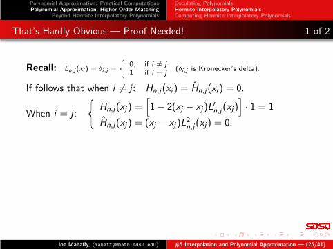
That’s Hardly Obvious — Proof Needed! 1 of 2
Recall: Ln,j (xi ) = δi,j =
0, if i 6= j
1 if i = j(δi,j is Kronecker’s delta).
If follows that when i 6= j : Hn,j(xi ) = Hn,j(xi ) = 0.
Joe Mahaffy, 〈[email protected]〉 #5 Interpolation and Polynomial Approximation — (25/41)
Polynomial Approximation: Practical ComputationsPolynomial Approximation, Higher Order Matching
Beyond Hermite Interpolatory Polynomials
Osculating PolynomialsHermite Interpolatory PolynomialsComputing Hermite Interpolatory Polynomials
That’s Hardly Obvious — Proof Needed! 1 of 2
Recall: Ln,j (xi ) = δi,j =
0, if i 6= j
1 if i = j(δi,j is Kronecker’s delta).
If follows that when i 6= j : Hn,j(xi ) = Hn,j(xi ) = 0.
When i = j :
{
Hn,j(xj) =[
1 − 2(xj − xj)L′n,j(xj)
]
· 1 = 1
Hn,j(xj) = (xj − xj)L2n,j(xj) = 0.
Joe Mahaffy, 〈[email protected]〉 #5 Interpolation and Polynomial Approximation — (25/41)

Polynomial Approximation: Practical ComputationsPolynomial Approximation, Higher Order Matching
Beyond Hermite Interpolatory Polynomials
Osculating PolynomialsHermite Interpolatory PolynomialsComputing Hermite Interpolatory Polynomials
That’s Hardly Obvious — Proof Needed! 1 of 2
Recall: Ln,j (xi ) = δi,j =
0, if i 6= j
1 if i = j(δi,j is Kronecker’s delta).
If follows that when i 6= j : Hn,j(xi ) = Hn,j(xi ) = 0.
When i = j :
{
Hn,j(xj) =[
1 − 2(xj − xj)L′n,j(xj)
]
· 1 = 1
Hn,j(xj) = (xj − xj)L2n,j(xj) = 0.
Thus, H2n+1(xj) = f(xj).
H′n,j (x) = [−2L′
n,j (xj )]L2n,j (x) + [1 − 2(x − xj )L
′n,j (xj )] · 2Ln,j (x)L′
n,j (x)
= Ln,j (x)h
−2L′n,j (xj )Ln,j (x) + [1 − 2(x − xj )L
′n,j (xj )] · 2(x)L′
n,j
i
Since Ln,j(x) is a factor in H ′n,j(x): H ′
n,j(xi ) = 0 when i 6= j .
Joe Mahaffy, 〈[email protected]〉 #5 Interpolation and Polynomial Approximation — (25/41)

Polynomial Approximation: Practical ComputationsPolynomial Approximation, Higher Order Matching
Beyond Hermite Interpolatory Polynomials
Osculating PolynomialsHermite Interpolatory PolynomialsComputing Hermite Interpolatory Polynomials
Proof, continued...
H′n,j (xj ) = [−2L′
n,j (xj )] L2n,j (xj )
| {z }
1
+ [1 − 2 (xj − xj )| {z }
0
L′n,j (xj )] · 2 Ln,j (xj )
| {z }
1
L′n,j (xj )
= −2L′n,j (xj ) + 1 · 2 · L′
n,j (xj ) = 0
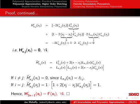
Joe Mahaffy, 〈[email protected]〉 #5 Interpolation and Polynomial Approximation — (26/41)

Polynomial Approximation: Practical ComputationsPolynomial Approximation, Higher Order Matching
Beyond Hermite Interpolatory Polynomials
Osculating PolynomialsHermite Interpolatory PolynomialsComputing Hermite Interpolatory Polynomials
Proof, continued...
H′n,j (xj ) = [−2L′
n,j (xj )] L2n,j (xj )
| {z }
1
+ [1 − 2 (xj − xj )| {z }
0
L′n,j (xj )] · 2 Ln,j (xj )
| {z }
1
L′n,j (xj )
= −2L′n,j (xj ) + 1 · 2 · L′
n,j (xj ) = 0
i.e. H′n,j(xi) = 0, ∀i.
H′n,j (x) = L2
n,j (x) + 2(x − xj )Ln,j (x)L′n,j (x)
= Ln,j (x)h
Ln,j (x) + 2(x − xj )L′n,j (x)
i
If i 6= j : H ′n,j(xi ) = 0, since Ln,j(xi ) = δi ,j .
If i = j : H ′n,j(xj) = 1 ·
[
1 + 2(xj − xj)L′n,j(xj)
]
= 1.
Joe Mahaffy, 〈[email protected]〉 #5 Interpolation and Polynomial Approximation — (26/41)
Polynomial Approximation: Practical ComputationsPolynomial Approximation, Higher Order Matching
Beyond Hermite Interpolatory Polynomials
Osculating PolynomialsHermite Interpolatory PolynomialsComputing Hermite Interpolatory Polynomials
Proof, continued...
H′n,j (xj ) = [−2L′
n,j (xj )] L2n,j (xj )
| {z }
1
+ [1 − 2 (xj − xj )| {z }
0
L′n,j (xj )] · 2 Ln,j (xj )
| {z }
1
L′n,j (xj )
= −2L′n,j (xj ) + 1 · 2 · L′
n,j (xj ) = 0
i.e. H′n,j(xi) = 0, ∀i.
H′n,j (x) = L2
n,j (x) + 2(x − xj )Ln,j (x)L′n,j (x)
= Ln,j (x)h
Ln,j (x) + 2(x − xj )L′n,j (x)
i
If i 6= j : H ′n,j(xi ) = 0, since Ln,j(xi ) = δi ,j .
If i = j : H ′n,j(xj) = 1 ·
[
1 + 2(xj − xj)L′n,j(xj)
]
= 1.
Hence, H′2n+1(xi) = f ′(xi), ∀i. ¤
Joe Mahaffy, 〈[email protected]〉 #5 Interpolation and Polynomial Approximation — (26/41)

Polynomial Approximation: Practical ComputationsPolynomial Approximation, Higher Order Matching
Beyond Hermite Interpolatory Polynomials
Osculating PolynomialsHermite Interpolatory PolynomialsComputing Hermite Interpolatory Polynomials
Uniqueness Proof
Assume there is a second polynomial G (x) (of degree≤ 2n + 1) interpolating the same data.
Joe Mahaffy, 〈[email protected]〉 #5 Interpolation and Polynomial Approximation — (27/41)
Polynomial Approximation: Practical ComputationsPolynomial Approximation, Higher Order Matching
Beyond Hermite Interpolatory Polynomials
Osculating PolynomialsHermite Interpolatory PolynomialsComputing Hermite Interpolatory Polynomials
Uniqueness Proof
Assume there is a second polynomial G (x) (of degree≤ 2n + 1) interpolating the same data.
Define R(x) = H2n+1(x) − G (x).
Joe Mahaffy, 〈[email protected]〉 #5 Interpolation and Polynomial Approximation — (27/41)

Polynomial Approximation: Practical ComputationsPolynomial Approximation, Higher Order Matching
Beyond Hermite Interpolatory Polynomials
Osculating PolynomialsHermite Interpolatory PolynomialsComputing Hermite Interpolatory Polynomials
Uniqueness Proof
Assume there is a second polynomial G (x) (of degree≤ 2n + 1) interpolating the same data.
Define R(x) = H2n+1(x) − G (x).
Then by construction R(xi ) = R ′(xi ) = 0, i.e. all the xi ’s arezeros of multiplicity at least 2.
This can only be true if R(x) = q(x)∏n
i=0(x − xi )2, for some
q(x).
If q(x) 6≡ 0 then the degree of R(x) is ≥ 2n + 2, which is acontradiction.
Hence q(x) ≡ 0 ⇒ R(x) ≡ 0 ⇒ H2n+1(x) is unique. ¤
Joe Mahaffy, 〈[email protected]〉 #5 Interpolation and Polynomial Approximation — (27/41)

Polynomial Approximation: Practical ComputationsPolynomial Approximation, Higher Order Matching
Beyond Hermite Interpolatory Polynomials
Osculating PolynomialsHermite Interpolatory PolynomialsComputing Hermite Interpolatory Polynomials
Main Use of Hermite Interpolatory Polynomials
One of the primary applications of Hermite Interpolatory Polynomials isthe development of Gaussian quadrature for numerical integration. (Tobe revisited later this semester.)
The most commonly seen Hermite interpolatory polynomial is the cubicone, which satisfies
H3(x0) = f (x0), H ′
3(x0) = f ′(x0)H3(x1) = f (x1), H ′
3(x1) = f ′(x1).
it can be written explicitly as
H3(x) =[
1 + 2 x−x0
x1−x0
] [
x1−xx1−x0
]2
f (x0) + (x − x0)[
x1−xx1−x0
]2
f ′(x0)
+[
1 + 2 x1−xx1−x0
] [
x−x0
x1−x0
]2
f (x1) + (x − x1)[
x−x0
x1−x0
]2
f ′(x1).
It appears in some optimization algorithms (see Math 693a, linesearchalgorithms.)
Joe Mahaffy, 〈[email protected]〉 #5 Interpolation and Polynomial Approximation — (28/41)

Polynomial Approximation: Practical ComputationsPolynomial Approximation, Higher Order Matching
Beyond Hermite Interpolatory Polynomials
Osculating PolynomialsHermite Interpolatory PolynomialsComputing Hermite Interpolatory Polynomials
Computing from the Definition is Tedious!
However, there is good news: we can re-use the algorithm for Newton’sInterpolatory Divided Difference Formula with some modifications inthe initialization.
We “double” the number of points, i.e. let
{y0, y1, . . . , y2n+1} = {x0, x0 + ǫ, x1, x1 + ǫ, . . . , xn, xn + ǫ}
Set up the divided difference table (up to the first divided differences),and let ǫ → 0 (formally), and identify:
f ′(xi ) = limǫ→0
f [xi + ǫ] − f [xi ]
ǫ,
to get the table [next slide]...
Joe Mahaffy, 〈[email protected]〉 #5 Interpolation and Polynomial Approximation — (29/41)

Polynomial Approximation: Practical ComputationsPolynomial Approximation, Higher Order Matching
Beyond Hermite Interpolatory Polynomials
Osculating PolynomialsHermite Interpolatory PolynomialsComputing Hermite Interpolatory Polynomials
Hermite Interpolatory Polynomial using Modified Newton Divided Differences
y f(x) 1st Div. Diff. 2nd Div. Diff. 3rd Div. Diff.y0 = x0 f [y0]
f [y0, y1] = f ′(y0)y1 = x0 f [y1] f [y0, y1, y2]
f [y1, y2] f [y0, y1, y2, y3]y2 = x1 f [y2] f [y1, y2, y3]
f [y2, y3] = f ′(y2) f [y1, y2, y3, y4]y3 = x1 f [y3] f [y2, y3, y4]
f [y3, y4] f [y2, y3, y4, y5]y4 = x2 f [y4] f [y3, y4, y5]
f [y4, y5] = f ′(y4) f [y3, y4, y5, y6]y5 = x2 f [y5] f [y4, y5, y6]
f [y5, y6] f [y4, y5, y6, y7]y6 = x3 f [y6] f [y5, y6, y7]
f [y6, y7] = f ′(y6) f [y5, y6, y7, y8]y7 = x3 f [y7] f [y6, y7, y8]
f [y7, y8] f [y6, y7, y8, y9]y8 = x4 f [y8] f [y7, y8, y9]
f [y8, y9] = f ′(y8)y9 = x4 f [y9]
Joe Mahaffy, 〈[email protected]〉 #5 Interpolation and Polynomial Approximation — (30/41)

Polynomial Approximation: Practical ComputationsPolynomial Approximation, Higher Order Matching
Beyond Hermite Interpolatory Polynomials
Osculating PolynomialsHermite Interpolatory PolynomialsComputing Hermite Interpolatory Polynomials
H3(x) revisited...
Old notation
H3(x) =[
1 + 2 x−x0
x1−x0
] [
x1−xx1−x0
]2
f (x0) +[
1 + 2 x1−xx1−x0
] [
x−x0
x1−x0
]2
f (x1)
+ (x − x0)[
x1−xx1−x0
]2
f ′(x0) + (x − x1)[
x−x0
x1−x0
]2
f ′(x1).
Divided difference notation
H3(x) = f (x0) + f ′(x0)(x − x0) + f [x0, x0, x1](x − x0)2
+ f [x0, x0, x1, x1](x − x0)2(x − x1).
Or with the y ’s...
H3(x) = f (y0) + f ′(y0)(x − y0) + f [y0, y1, y2](x − y0)(x − y1)+ f [y0, y1, y2, y3](x − y1)(x − y2)(x − y3).
Joe Mahaffy, 〈[email protected]〉 #5 Interpolation and Polynomial Approximation — (31/41)
Polynomial Approximation: Practical ComputationsPolynomial Approximation, Higher Order Matching
Beyond Hermite Interpolatory Polynomials
Osculating PolynomialsHermite Interpolatory PolynomialsComputing Hermite Interpolatory Polynomials
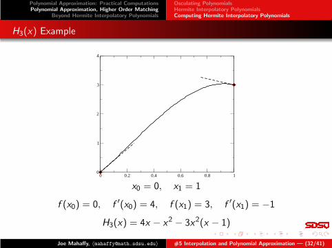
H3(x) Example
0 0.2 0.4 0.6 0.8 10
1
2
3
4
x0 = 0, x1 = 1
f (x0) = 0, f ′(x0) = 4, f (x1) = 3, f ′(x1) = −1
H3(x) = 4x − x2 − 3x2(x − 1)
Joe Mahaffy, 〈[email protected]〉 #5 Interpolation and Polynomial Approximation — (32/41)

Polynomial Approximation: Practical ComputationsPolynomial Approximation, Higher Order Matching
Beyond Hermite Interpolatory Polynomials
Osculating PolynomialsHermite Interpolatory PolynomialsComputing Hermite Interpolatory Polynomials
H3(x) Example — Not Very Pretty Computations
Example
x0 = 0; x1 = 1; % This is the datafv0 = 0; fpv0 = 4;fv1 = 3; fpv1 = -1;
y0 = x0; f0=fv0; % Initializing the tabley1 = x0; f1=fv0;y2 = x1; f2=fv1;y3 = x1; f3=fv1;
f01 = fpv0; % First divided differencesf12 = (f2-f1)/(y2-y1);f23 = fpv1;
f012 = (f12-f01)/(y2-y0); % Second divided differencesf123 = (f23-f12)/(y3-y1);
f0123 = (f123-f012)/(y3-y0); % Third divided difference
x=(0:0.01:1)’;
H3 = f0 + f01*(x-y0) + f012*(x-y0).*(x-y1) + ...
f0123*(x-y0).*(x-y1).* (x-y2);
Joe Mahaffy, 〈[email protected]〉 #5 Interpolation and Polynomial Approximation — (33/41)

Polynomial Approximation: Practical ComputationsPolynomial Approximation, Higher Order Matching
Beyond Hermite Interpolatory Polynomials
Osculating PolynomialsHermite Interpolatory PolynomialsComputing Hermite Interpolatory Polynomials
Algorithm: Hermite Interpolation
Algorithm: Hermite Interpolation, Part #1
Given the data points (xi , f (xi ), f′(xi )), i = 0, . . . , n.
Step 1: FOR i=0:n
y2i = xi, Q2i,0 = f (xi ), y2i+1 = xi, Q2i+1,0 = f (xi )Q2i+1,1 = f ′(xi )IF i > 0
Q2i,1 =Qi,0 − Qi−1,0
y2i − y2i−1END
END
Joe Mahaffy, 〈[email protected]〉 #5 Interpolation and Polynomial Approximation — (34/41)

Polynomial Approximation: Practical ComputationsPolynomial Approximation, Higher Order Matching
Beyond Hermite Interpolatory Polynomials
Osculating PolynomialsHermite Interpolatory PolynomialsComputing Hermite Interpolatory Polynomials
Algorithm: Hermite Interpolation
Algorithm: Hermite Interpolation, Part #2
Step 2: FOR i = 2 : (2n + 1)FOR j = 2 : i
Qi,j =Qi,j−i − Qi−1,j−1
yi − yi−j
.
END
END
Result: qi = Qi,i , i = 0, . . . , 2n + 1 now contains the coefficients for
H2n+1(x) = q0 +
2n+1∑
k=1
qi
k−1∏
j=0
(x − yj)
.
Joe Mahaffy, 〈[email protected]〉 #5 Interpolation and Polynomial Approximation — (35/41)

Polynomial Approximation: Practical ComputationsPolynomial Approximation, Higher Order Matching
Beyond Hermite Interpolatory Polynomials
Higher Order Osculating Polynomials 1 of 3
So far we have seen the osculating polynomials of order 0 — theLagrange polynomial, and of order 1 — the Hermite interpolatorypolynomial.
It turns out that generating osculating polynomials of higher orderis fairly straight-forward; — and we use Newton’s divideddifferences to generate those as well.
Joe Mahaffy, 〈[email protected]〉 #5 Interpolation and Polynomial Approximation — (36/41)

Polynomial Approximation: Practical ComputationsPolynomial Approximation, Higher Order Matching
Beyond Hermite Interpolatory Polynomials
Higher Order Osculating Polynomials 1 of 3
So far we have seen the osculating polynomials of order 0 — theLagrange polynomial, and of order 1 — the Hermite interpolatorypolynomial.
It turns out that generating osculating polynomials of higher orderis fairly straight-forward; — and we use Newton’s divideddifferences to generate those as well.
Given a set of points {xk}nk=0, and {f (ℓ)(xk)}n,ℓk
k=0,ℓ=0; i.e. thefunction values, as well as the first ℓk derivatives of f in xk . (Notethat we can specify a different number of derivatives in each point.)
Set up the Newton-divided-difference table, and put in (ℓk + 1)duplicate entries of each point xk , as well as its function valuef (xk).
Joe Mahaffy, 〈[email protected]〉 #5 Interpolation and Polynomial Approximation — (36/41)

Polynomial Approximation: Practical ComputationsPolynomial Approximation, Higher Order Matching
Beyond Hermite Interpolatory Polynomials
Higher Order Osculating Polynomials 2 of 3
Run the computation of Newton’s divided differences as usual;with the following exception:
Whenever a zero-denominator is encountered — i.e. the divideddifference for that entry cannot be computed due to duplica-tion of a point — use a derivative instead. For mth divideddifferences, use 1
m! f(m)(xk).
On the next slide we see the setup for two point in which twoderivatives are prescribed.
Joe Mahaffy, 〈[email protected]〉 #5 Interpolation and Polynomial Approximation — (37/41)

Polynomial Approximation: Practical ComputationsPolynomial Approximation, Higher Order Matching
Beyond Hermite Interpolatory Polynomials
Higher Order Osculating Polynomials 3 of 3
y f(x) 1st Div. Diff. 2nd Div. Diff. 3rd Div. Diff.y0 = x0 f [y0]
f [y0, y1] = f ′(x0)y1 = x0 f [y1] f [y0, y1, y2] = 1
2f ′′(x0)
f [y1, y2] = f ′(x0) f [y0, y1, y2, y3]y2 = x0 f [y2] f [y1, y2, y3]
f [y2, y3] f [y1, y2, y3, y4]y3 = x1 f [y3] f [y2, y3, y4]
f [y3, y4] = f ′(x1) f [y2, y3, y4, y5]y4 = x1 f [y4] f [y3, y4, y5] = 1
2f ′′(x1)
f [y4, y5] = f ′(x1)y5 = x1 f [y5]
3rd and higher order divided differences are computed “as usual”in this case.
On the next slide we see four examples of 2nd order osculatingpolynomials.
Joe Mahaffy, 〈[email protected]〉 #5 Interpolation and Polynomial Approximation — (38/41)

Polynomial Approximation: Practical ComputationsPolynomial Approximation, Higher Order Matching
Beyond Hermite Interpolatory Polynomials
Examples...
−1 −0.8 −0.6 −0.4 −0.2 0 0.2 0.4 0.6 0.8 1
−1
−0.8
−0.6
−0.4
−0.2
0
0.2
0.4
0.6
0.8
1
f(−1) = +1.00
df(−1) = +1.00
ddf(−1) = +0.00
f(1) = −1.00
df(1) = −1.00
ddf(1) = +0.00
f(0) = +0.00
df(0) = +1.00
ddf(0) = +0.00
Osculating Polynomials
Joe Mahaffy, 〈[email protected]〉 #5 Interpolation and Polynomial Approximation — (39/41)

Polynomial Approximation: Practical ComputationsPolynomial Approximation, Higher Order Matching
Beyond Hermite Interpolatory Polynomials
Examples...
−1 −0.8 −0.6 −0.4 −0.2 0 0.2 0.4 0.6 0.8 1
−1
−0.8
−0.6
−0.4
−0.2
0
0.2
0.4
0.6
0.8
1
f(−1) = +1.00
df(−1) = +1.00
ddf(−1) = +0.00
f(1) = −1.00
df(1) = −1.00
ddf(1) = +0.00
f(0) = +0.00
df(0) = −1.00
ddf(0) = +0.00
Osculating Polynomials
Joe Mahaffy, 〈[email protected]〉 #5 Interpolation and Polynomial Approximation — (39/41)

Polynomial Approximation: Practical ComputationsPolynomial Approximation, Higher Order Matching
Beyond Hermite Interpolatory Polynomials
Examples...
−1 −0.8 −0.6 −0.4 −0.2 0 0.2 0.4 0.6 0.8 1
−1
−0.5
0
0.5
1
f(−1) = +1.00
df(−1) = +2.00
ddf(−1) = −1.00
f(1) = −1.00
df(1) = +1.00
ddf(1) = +3.00
f(0) = +0.00
df(0) = +0.00
ddf(0) = +10.00
Osculating Polynomials
Joe Mahaffy, 〈[email protected]〉 #5 Interpolation and Polynomial Approximation — (39/41)

Polynomial Approximation: Practical ComputationsPolynomial Approximation, Higher Order Matching
Beyond Hermite Interpolatory Polynomials
Examples...
−1 −0.8 −0.6 −0.4 −0.2 0 0.2 0.4 0.6 0.8 1
−1
−0.8
−0.6
−0.4
−0.2
0
0.2
0.4
0.6
0.8
1
f(−1) = +1.00
df(−1) = −1.00
ddf(−1) = −10.00
f(1) = −1.00
df(1) = −1.00
ddf(1) = +10.00
f(0) = +0.00
df(0) = −1.00
ddf(0) = −10.00
Osculating Polynomials
Joe Mahaffy, 〈[email protected]〉 #5 Interpolation and Polynomial Approximation — (39/41)

Polynomial Approximation: Practical ComputationsPolynomial Approximation, Higher Order Matching
Beyond Hermite Interpolatory Polynomials
Examples...
−1 −0.8 −0.6 −0.4 −0.2 0 0.2 0.4 0.6 0.8 1
−1
−0.8
−0.6
−0.4
−0.2
0
0.2
0.4
0.6
0.8
1
f(−1) = +1.00
df(−1) = +1.00
ddf(−1) = +0.00
f(1) = −1.00
df(1) = −1.00
ddf(1) = +0.00
f(0) = +0.00
df(0) = +1.00
ddf(0) = +0.00
Osculating Polynomials
−1 −0.8 −0.6 −0.4 −0.2 0 0.2 0.4 0.6 0.8 1
−1
−0.8
−0.6
−0.4
−0.2
0
0.2
0.4
0.6
0.8
1
f(−1) = +1.00
df(−1) = +1.00
ddf(−1) = +0.00
f(1) = −1.00
df(1) = −1.00
ddf(1) = +0.00
f(0) = +0.00
df(0) = −1.00
ddf(0) = +0.00
Osculating Polynomials
−1 −0.8 −0.6 −0.4 −0.2 0 0.2 0.4 0.6 0.8 1
−1
−0.5
0
0.5
1
f(−1) = +1.00
df(−1) = +2.00
ddf(−1) = −1.00
f(1) = −1.00
df(1) = +1.00
ddf(1) = +3.00
f(0) = +0.00
df(0) = +0.00
ddf(0) = +10.00
Osculating Polynomials
−1 −0.8 −0.6 −0.4 −0.2 0 0.2 0.4 0.6 0.8 1
−1
−0.8
−0.6
−0.4
−0.2
0
0.2
0.4
0.6
0.8
1
f(−1) = +1.00
df(−1) = −1.00
ddf(−1) = −10.00
f(1) = −1.00
df(1) = −1.00
ddf(1) = +10.00
f(0) = +0.00
df(0) = −1.00
ddf(0) = −10.00
Osculating Polynomials
Joe Mahaffy, 〈[email protected]〉 #5 Interpolation and Polynomial Approximation — (39/41)

Polynomial Approximation: Practical ComputationsPolynomial Approximation, Higher Order Matching
Beyond Hermite Interpolatory Polynomials
We have encountered methods by these fellows
Sir Isaac Newton, 4 Jan 1643 (Woolsthorpe, Lincolnshire, England) — 31March 1727.
Joseph-Louis Lagrange, 25 Jan 1736 (Turin, Sardinia-Piedmont (nowItaly)) — 10 April 1813.
Johann Carl Friedrich Gauss, 30 April 1777 (Brunswick, Duchy ofBrunswick (now Germany)) — 23 Feb 1855.
Charles Hermite, 24 Dec 1822 (Dieuze, Lorraine, France) — 14 Jan 1901.
The class website contains links to short bios for these (and other)mathematicians, click on Mathematics Personae, who have contributedto the material covered in this class. It makes for interesting reading andputs mathematics into a historical and political context.
Joe Mahaffy, 〈[email protected]〉 #5 Interpolation and Polynomial Approximation — (40/41)
Top Related