


Languages
Pages
Legal

distributed graph algorithmsGeneralized Architecture For Some Graph Problems
Abhilash Kumar and Saurav KumarNovember 10, 2015
Indian Institute of Technology Kanpur

problem statement
problem statement
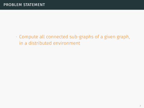
∙ Compute all connected sub-graphs of a given graph,in a distributed environment
∙ Develop a generalized architecture to solve similargraph problems
2
problem statement
∙ Compute all connected sub-graphs of a given graph,in a distributed environment
∙ Develop a generalized architecture to solve similargraph problems
2

motivation
motivation
∙ Exponential number of connected sub-graphs of agiven graph
∙ Necessity to build distributed systems which utilizethe worldwide plethora of distributed resources
4
motivation
∙ Exponential number of connected sub-graphs of agiven graph
∙ Necessity to build distributed systems which utilizethe worldwide plethora of distributed resources
4

approach
approach
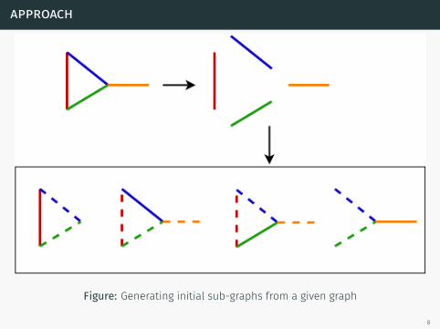
Insights∙ Connected sub-graphs exhibit sub-structure
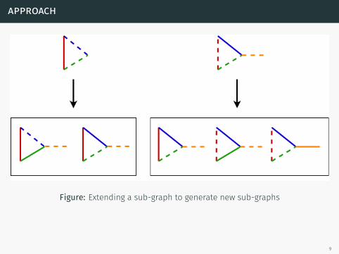
∙ Extend smaller sub-graphs by adding an outgoing edge togenerate larger sub-graphs
∙ Base cases are sub-graphs represented by all the edges of thegraph
6
approach
Insights∙ Connected sub-graphs exhibit sub-structure
∙ Extend smaller sub-graphs by adding an outgoing edge togenerate larger sub-graphs
∙ Base cases are sub-graphs represented by all the edges of thegraph
6
approach
Insights∙ Connected sub-graphs exhibit sub-structure
∙ Extend smaller sub-graphs by adding an outgoing edge togenerate larger sub-graphs
∙ Base cases are sub-graphs represented by all the edges of thegraph
6
approach
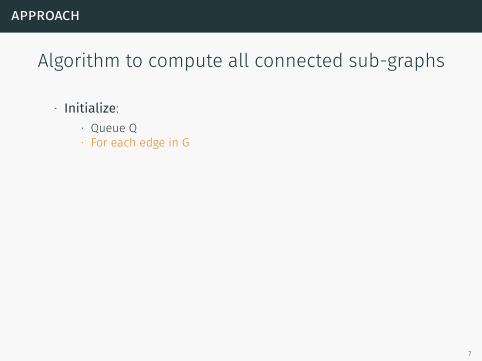
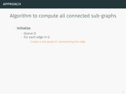
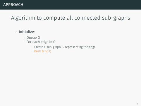
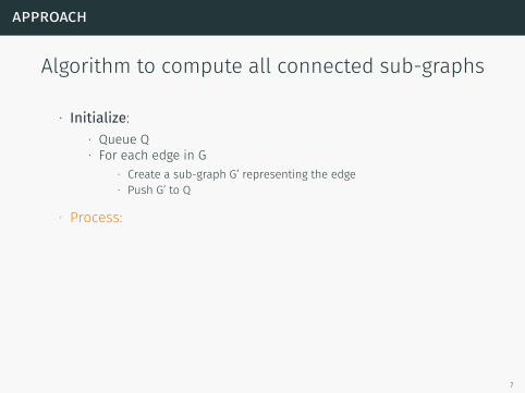
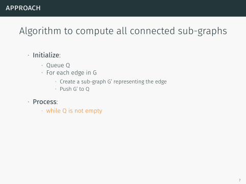
Algorithm to compute all connected sub-graphs
∙ Initialize:
∙ Queue Q∙ For each edge in G
∙ Create a sub-graph G’ representing the edge∙ Push G’ to Q
∙ Process:
∙ while Q is not empty
∙ G = Q.pop()∙ Save G∙ For each outgoing edge E of G
G’ = G U Eif G’ has not been seen yet
Push G’ to Q
7
approach
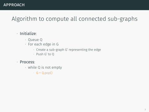
Algorithm to compute all connected sub-graphs
∙ Initialize:∙ Queue Q
∙ For each edge in G
∙ Create a sub-graph G’ representing the edge∙ Push G’ to Q
∙ Process:
∙ while Q is not empty
∙ G = Q.pop()∙ Save G∙ For each outgoing edge E of G
G’ = G U Eif G’ has not been seen yet
Push G’ to Q
7
approach
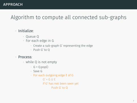
Algorithm to compute all connected sub-graphs
∙ Initialize:∙ Queue Q∙ For each edge in G
∙ Create a sub-graph G’ representing the edge∙ Push G’ to Q
∙ Process:
∙ while Q is not empty
∙ G = Q.pop()∙ Save G∙ For each outgoing edge E of G
G’ = G U Eif G’ has not been seen yet
Push G’ to Q
7
approach
Algorithm to compute all connected sub-graphs
∙ Initialize:∙ Queue Q∙ For each edge in G
∙ Create a sub-graph G’ representing the edge
∙ Push G’ to Q
∙ Process:
∙ while Q is not empty
∙ G = Q.pop()∙ Save G∙ For each outgoing edge E of G
G’ = G U Eif G’ has not been seen yet
Push G’ to Q
7
approach
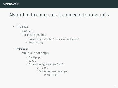
Algorithm to compute all connected sub-graphs
∙ Initialize:∙ Queue Q∙ For each edge in G
∙ Create a sub-graph G’ representing the edge∙ Push G’ to Q
∙ Process:
∙ while Q is not empty
∙ G = Q.pop()∙ Save G∙ For each outgoing edge E of G
G’ = G U Eif G’ has not been seen yet
Push G’ to Q
7
approach
Algorithm to compute all connected sub-graphs
∙ Initialize:∙ Queue Q∙ For each edge in G
∙ Create a sub-graph G’ representing the edge∙ Push G’ to Q
∙ Process:
∙ while Q is not empty
∙ G = Q.pop()∙ Save G∙ For each outgoing edge E of G
G’ = G U Eif G’ has not been seen yet
Push G’ to Q
7
approach
Algorithm to compute all connected sub-graphs
∙ Initialize:∙ Queue Q∙ For each edge in G
∙ Create a sub-graph G’ representing the edge∙ Push G’ to Q
∙ Process:∙ while Q is not empty
∙ G = Q.pop()∙ Save G∙ For each outgoing edge E of G
G’ = G U Eif G’ has not been seen yet
Push G’ to Q
7
approach
Algorithm to compute all connected sub-graphs
∙ Initialize:∙ Queue Q∙ For each edge in G
∙ Create a sub-graph G’ representing the edge∙ Push G’ to Q
∙ Process:∙ while Q is not empty
∙ G = Q.pop()
∙ Save G∙ For each outgoing edge E of G
G’ = G U Eif G’ has not been seen yet
Push G’ to Q
7

approach
Algorithm to compute all connected sub-graphs
∙ Initialize:∙ Queue Q∙ For each edge in G
∙ Create a sub-graph G’ representing the edge∙ Push G’ to Q
∙ Process:∙ while Q is not empty
∙ G = Q.pop()∙ Save G
∙ For each outgoing edge E of GG’ = G U Eif G’ has not been seen yet
Push G’ to Q
7
approach
Algorithm to compute all connected sub-graphs
∙ Initialize:∙ Queue Q∙ For each edge in G
∙ Create a sub-graph G’ representing the edge∙ Push G’ to Q
∙ Process:∙ while Q is not empty
∙ G = Q.pop()∙ Save G∙ For each outgoing edge E of G
G’ = G U Eif G’ has not been seen yet
Push G’ to Q
7

approach
Algorithm to compute all connected sub-graphs
∙ Initialize:∙ Queue Q∙ For each edge in G
∙ Create a sub-graph G’ representing the edge∙ Push G’ to Q
∙ Process:∙ while Q is not empty
∙ G = Q.pop()∙ Save G∙ For each outgoing edge E of G
G’ = G U Eif G’ has not been seen yet
Push G’ to Q
7
approach
Algorithm to compute all connected sub-graphs
∙ Initialize:∙ Queue Q∙ For each edge in G
∙ Create a sub-graph G’ representing the edge∙ Push G’ to Q
∙ Process:∙ while Q is not empty
∙ G = Q.pop()∙ Save G∙ For each outgoing edge E of G
G’ = G U Eif G’ has not been seen yet
Push G’ to Q
7
approach
Figure: Generating initial sub-graphs from a given graph
8
approach
Figure: Extending a sub-graph to generate new sub-graphs
9
approach
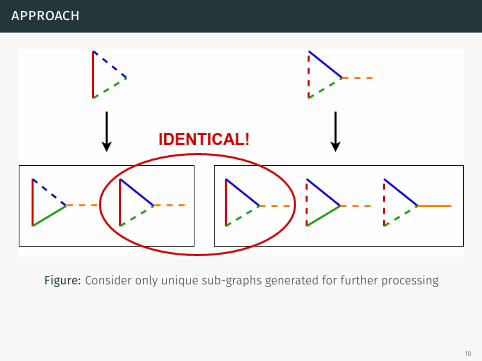
Figure: Consider only unique sub-graphs generated for further processing
10

architecture
architecture
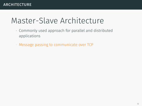
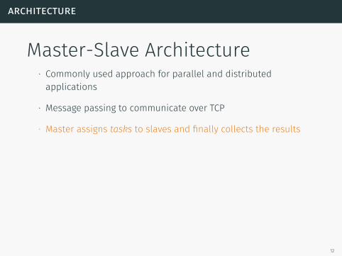
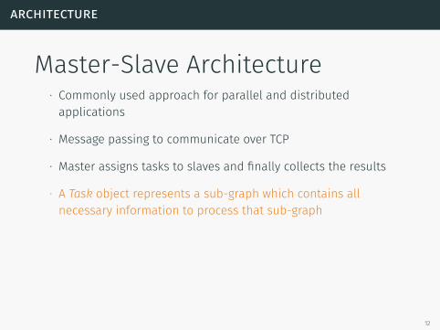
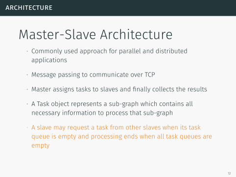
Master-Slave Architecture∙ Commonly used approach for parallel and distributedapplications
∙ Message passing to communicate over TCP
∙ Master assigns tasks to slaves and finally collects the results
∙ A Task object represents a sub-graph which contains allnecessary information to process that sub-graph
∙ A slave may request a task from other slaves when its taskqueue is empty and processing ends when all task queues areempty
12
architecture
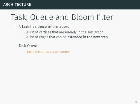
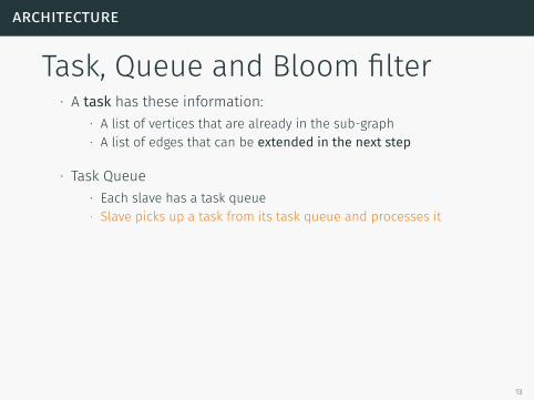
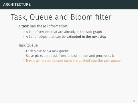
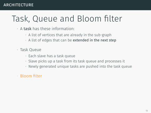
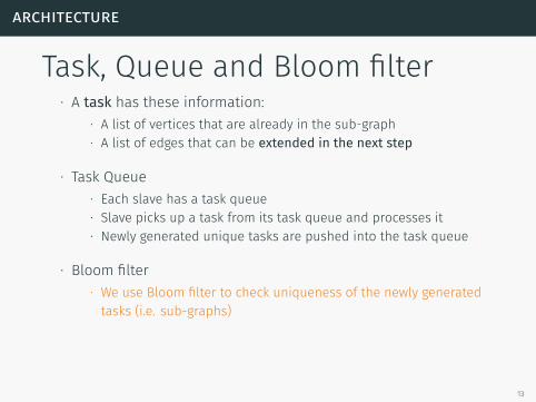
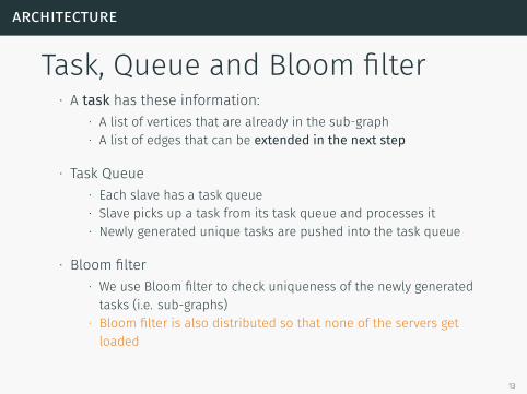
Task, Queue and Bloom filter∙ A task has these information:
∙ A list of vertices that are already in the sub-graph∙ A list of edges that can be extended in the next step
∙ Task Queue
∙ Each slave has a task queue∙ Slave picks up a task from its task queue and processes it∙ Newly generated unique tasks are pushed into the task queue
∙ Bloom filter
∙ We use Bloom filter to check uniqueness of the newly generatedtasks (i.e. sub-graphs)
∙ Bloom filter is also distributed so that none of the servers getloaded
13
architecture
Task, Queue and Bloom filter∙ A task has these information:
∙ A list of vertices that are already in the sub-graph
∙ A list of edges that can be extended in the next step
∙ Task Queue
∙ Each slave has a task queue∙ Slave picks up a task from its task queue and processes it∙ Newly generated unique tasks are pushed into the task queue
∙ Bloom filter
∙ We use Bloom filter to check uniqueness of the newly generatedtasks (i.e. sub-graphs)
∙ Bloom filter is also distributed so that none of the servers getloaded
13
architecture
Task, Queue and Bloom filter∙ A task has these information:
∙ A list of vertices that are already in the sub-graph∙ A list of edges that can be extended in the next step
∙ Task Queue
∙ Each slave has a task queue∙ Slave picks up a task from its task queue and processes it∙ Newly generated unique tasks are pushed into the task queue
∙ Bloom filter
∙ We use Bloom filter to check uniqueness of the newly generatedtasks (i.e. sub-graphs)
∙ Bloom filter is also distributed so that none of the servers getloaded
13
architecture
Task, Queue and Bloom filter∙ A task has these information:
∙ A list of vertices that are already in the sub-graph∙ A list of edges that can be extended in the next step
∙ Task Queue∙ Each slave has a task queue
∙ Slave picks up a task from its task queue and processes it∙ Newly generated unique tasks are pushed into the task queue
∙ Bloom filter
∙ We use Bloom filter to check uniqueness of the newly generatedtasks (i.e. sub-graphs)
∙ Bloom filter is also distributed so that none of the servers getloaded
13
architecture
Task, Queue and Bloom filter∙ A task has these information:
∙ A list of vertices that are already in the sub-graph∙ A list of edges that can be extended in the next step
∙ Task Queue∙ Each slave has a task queue∙ Slave picks up a task from its task queue and processes it
∙ Newly generated unique tasks are pushed into the task queue
∙ Bloom filter
∙ We use Bloom filter to check uniqueness of the newly generatedtasks (i.e. sub-graphs)
∙ Bloom filter is also distributed so that none of the servers getloaded
13
architecture
Task, Queue and Bloom filter∙ A task has these information:
∙ A list of vertices that are already in the sub-graph∙ A list of edges that can be extended in the next step
∙ Task Queue∙ Each slave has a task queue∙ Slave picks up a task from its task queue and processes it∙ Newly generated unique tasks are pushed into the task queue
∙ Bloom filter∙ We use Bloom filter to check uniqueness of the newly generatedtasks (i.e. sub-graphs)
∙ Bloom filter is also distributed so that none of the servers getloaded
13
architecture
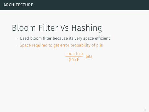
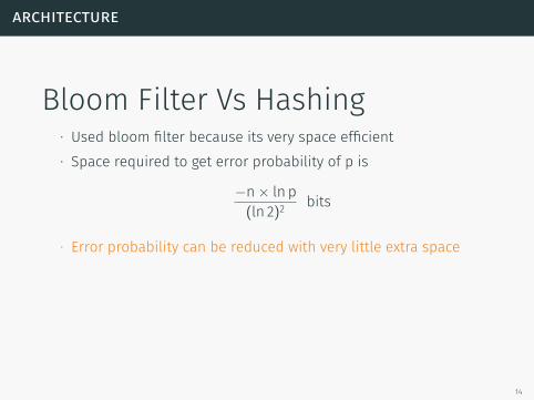
Bloom Filter Vs Hashing∙ Used bloom filter because its very space efficient
∙ Space required to get error probability of p is
−n× ln p(ln 2)2 bits
∙ Error probability can be reduced with very little extra space∙ Hashing can be used to make the algorithm deterministic∙ Bloom filter can also be parallelized whereas Hashing cannot be.
14
architecture
Bloom Filter Vs Hashing∙ Used bloom filter because its very space efficient∙ Space required to get error probability of p is
−n× ln p(ln 2)2 bits
∙ Error probability can be reduced with very little extra space∙ Hashing can be used to make the algorithm deterministic∙ Bloom filter can also be parallelized whereas Hashing cannot be.
14
architecture
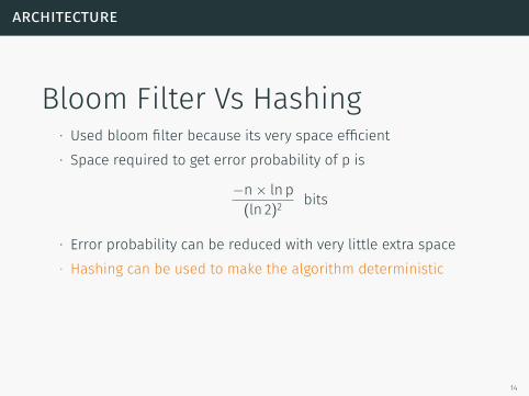
Bloom Filter Vs Hashing∙ Used bloom filter because its very space efficient∙ Space required to get error probability of p is
−n× ln p(ln 2)2 bits
∙ Error probability can be reduced with very little extra space
∙ Hashing can be used to make the algorithm deterministic∙ Bloom filter can also be parallelized whereas Hashing cannot be.
14
architecture
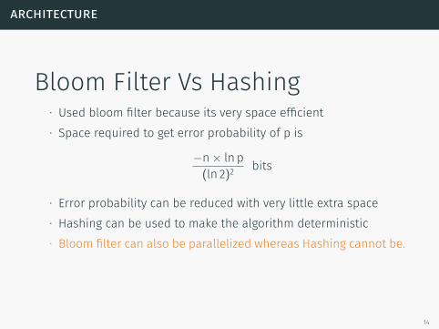
Bloom Filter Vs Hashing∙ Used bloom filter because its very space efficient∙ Space required to get error probability of p is
−n× ln p(ln 2)2 bits
∙ Error probability can be reduced with very little extra space∙ Hashing can be used to make the algorithm deterministic
∙ Bloom filter can also be parallelized whereas Hashing cannot be.
14
architecture
Bloom Filter Vs Hashing∙ Used bloom filter because its very space efficient∙ Space required to get error probability of p is
−n× ln p(ln 2)2 bits
∙ Error probability can be reduced with very little extra space∙ Hashing can be used to make the algorithm deterministic∙ Bloom filter can also be parallelized whereas Hashing cannot be.
14
architecture
How to use this architecture?∙ Two functions required: initialize and process
∙ Initialize generates initial tasks. Master randomly assigns thesetasks to the slaves.
∙ Process defines a procedure that will generate new tasks from agiven task (extend sub-graph in our case)
15
architecture
How to use this architecture?∙ Two functions required: initialize and process
∙ Initialize generates initial tasks. Master randomly assigns thesetasks to the slaves.
∙ Process defines a procedure that will generate new tasks from agiven task (extend sub-graph in our case)
15
architecture
How to use this architecture?∙ Two functions required: initialize and process
∙ Initialize generates initial tasks. Master randomly assigns thesetasks to the slaves.
∙ Process defines a procedure that will generate new tasks from agiven task (extend sub-graph in our case)
15

architecture
How to use this architecture?∙ Two functions required: initialize and process
∙ Initialize generates initial tasks. Master randomly assigns thesetasks to the slaves.
∙ Process defines a procedure that will generate new tasks from agiven task (extend sub-graph in our case)
15
architecture
How to use this architecture?∙ Two functions required: initialize and process
∙ Initialize generates initial tasks. Master randomly assigns thesetasks to the slaves.
∙ Process defines a procedure that will generate new tasks from agiven task (extend sub-graph in our case)
15
architecture
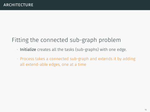
Fitting the connected sub-graph problem∙ Initialize creates all the tasks (sub-graphs) with one edge.
∙ Process takes a connected sub-graph and extends it by addingall extend-able edges, one at a time
16
architecture
Fitting the connected sub-graph problem∙ Initialize creates all the tasks (sub-graphs) with one edge.
∙ Process takes a connected sub-graph and extends it by addingall extend-able edges, one at a time
16

simulation
simulation
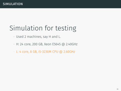
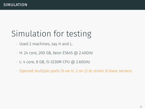
Simulation for testing∙ Used 2 machines, say H and L.
∙ H: 24 core, 200 GB, Xeon E5645 @ 2.40GHz
∙ L: 4 core, 8 GB, i5-3230M CPU @ 2.60GHz
∙ Opened multiple ports (6 on H, 2 on L) to mimic 8 slave servers.
18
simulation
Simulation for testing∙ Used 2 machines, say H and L.
∙ H: 24 core, 200 GB, Xeon E5645 @ 2.40GHz
∙ L: 4 core, 8 GB, i5-3230M CPU @ 2.60GHz
∙ Opened multiple ports (6 on H, 2 on L) to mimic 8 slave servers.
18
simulation
Simulation for testing∙ Used 2 machines, say H and L.
∙ H: 24 core, 200 GB, Xeon E5645 @ 2.40GHz
∙ L: 4 core, 8 GB, i5-3230M CPU @ 2.60GHz
∙ Opened multiple ports (6 on H, 2 on L) to mimic 8 slave servers.
18
simulation
Simulation for testing∙ Used 2 machines, say H and L.
∙ H: 24 core, 200 GB, Xeon E5645 @ 2.40GHz
∙ L: 4 core, 8 GB, i5-3230M CPU @ 2.60GHz
∙ Opened multiple ports (6 on H, 2 on L) to mimic 8 slave servers.
18
simulation
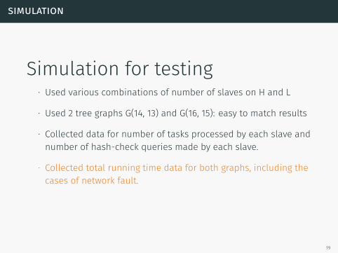
Simulation for testing∙ Used various combinations of number of slaves on H and L
∙ Used 2 tree graphs G(14, 13) and G(16, 15): easy to match results
∙ Collected data for number of tasks processed by each slave andnumber of hash-check queries made by each slave.
∙ Collected total running time data for both graphs, including thecases of network fault.
19
simulation
Simulation for testing∙ Used various combinations of number of slaves on H and L
∙ Used 2 tree graphs G(14, 13) and G(16, 15): easy to match results
∙ Collected data for number of tasks processed by each slave andnumber of hash-check queries made by each slave.
∙ Collected total running time data for both graphs, including thecases of network fault.
19

results
results
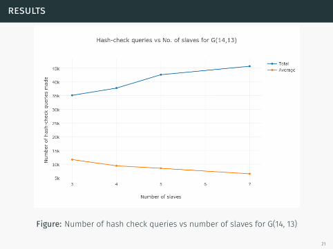
Figure: Number of hash check queries vs number of slaves for G(14, 13)
21
results
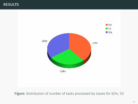
Figure: Distribution of number of tasks processed by slaves for G(14, 13)
22
results
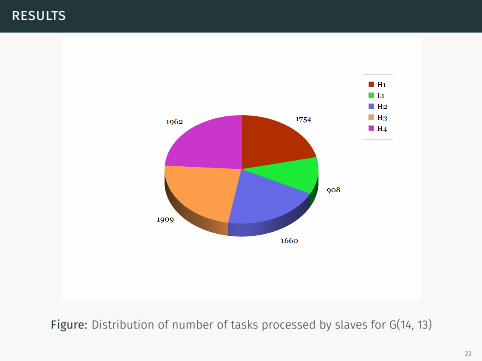
Figure: Distribution of number of tasks processed by slaves for G(14, 13)
23
results
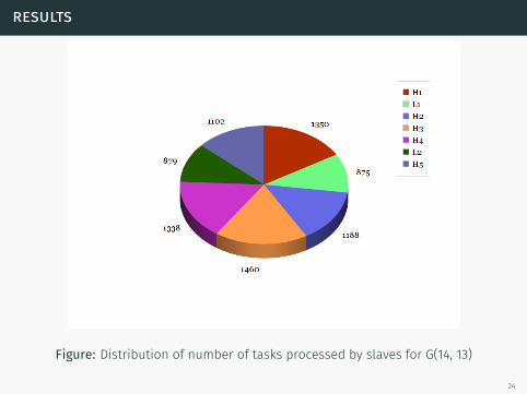
Figure: Distribution of number of tasks processed by slaves for G(14, 13)
24
results
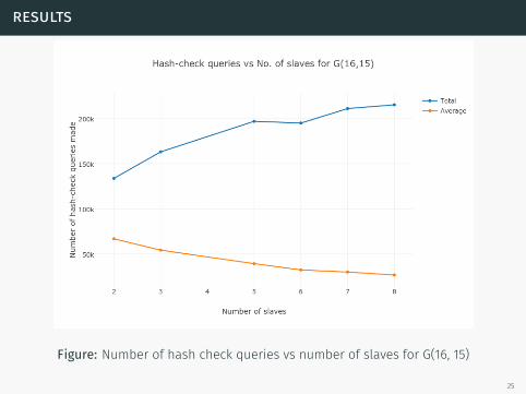
Figure: Number of hash check queries vs number of slaves for G(16, 15)
25
results
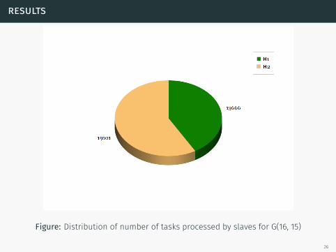
Figure: Distribution of number of tasks processed by slaves for G(16, 15)
26
results
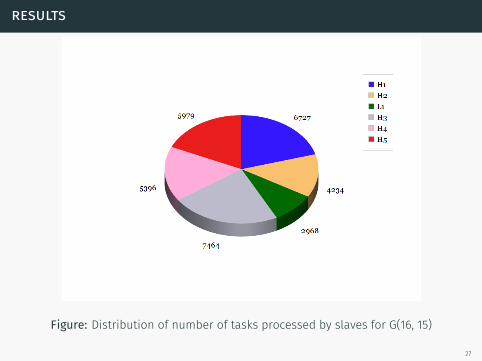
Figure: Distribution of number of tasks processed by slaves for G(16, 15)
27
results
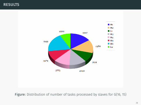
Figure: Distribution of number of tasks processed by slaves for G(16, 15)
28
results
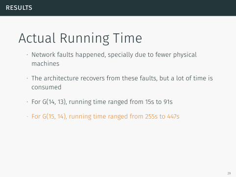
Actual Running Time∙ Network faults happened, specially due to fewer physicalmachines
∙ The architecture recovers from these faults, but a lot of time isconsumed
∙ For G(14, 13), running time ranged from 15s to 91s
∙ For G(15, 14), running time ranged from 255s to 447s
∙ These are the cases when process function doesn’t doadditional computation per subgraph.
29
results
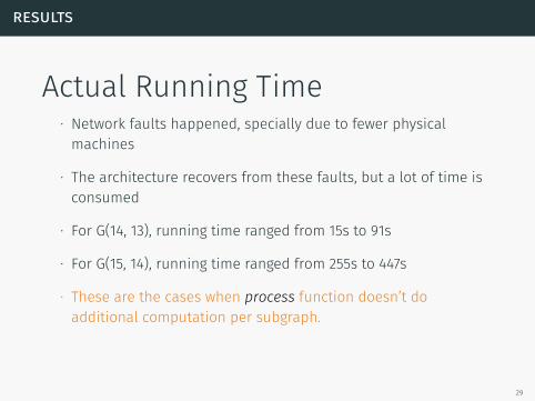
Actual Running Time∙ Network faults happened, specially due to fewer physicalmachines
∙ The architecture recovers from these faults, but a lot of time isconsumed
∙ For G(14, 13), running time ranged from 15s to 91s
∙ For G(15, 14), running time ranged from 255s to 447s
∙ These are the cases when process function doesn’t doadditional computation per subgraph.
29
results
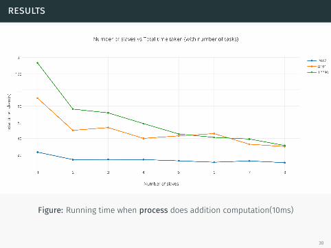
Figure: Running time when process does addition computation(10ms)
30
advantages
advantages
Advantages∙ Highly scalable
∙ More slaves can be added easily∙ Performance increases with number of slaves∙ Even distribution of tasks: efficient machines process more tasks
∙ Architecture is very reusable
∙ Many other problems can be solved using this architecture∙ Only need to provide 2 functions: initialize and process
∙ Network fault tolerant
32
advantages
Advantages∙ Highly scalable
∙ More slaves can be added easily
∙ Performance increases with number of slaves∙ Even distribution of tasks: efficient machines process more tasks
∙ Architecture is very reusable
∙ Many other problems can be solved using this architecture∙ Only need to provide 2 functions: initialize and process
∙ Network fault tolerant
32
advantages
Advantages∙ Highly scalable
∙ More slaves can be added easily∙ Performance increases with number of slaves
∙ Even distribution of tasks: efficient machines process more tasks
∙ Architecture is very reusable
∙ Many other problems can be solved using this architecture∙ Only need to provide 2 functions: initialize and process
∙ Network fault tolerant
32
advantages
Advantages∙ Highly scalable
∙ More slaves can be added easily∙ Performance increases with number of slaves∙ Even distribution of tasks: efficient machines process more tasks
∙ Architecture is very reusable
∙ Many other problems can be solved using this architecture∙ Only need to provide 2 functions: initialize and process
∙ Network fault tolerant
32
advantages
Advantages∙ Highly scalable
∙ More slaves can be added easily∙ Performance increases with number of slaves∙ Even distribution of tasks: efficient machines process more tasks
∙ Architecture is very reusable
∙ Many other problems can be solved using this architecture∙ Only need to provide 2 functions: initialize and process
∙ Network fault tolerant
32

advantages
Advantages∙ Highly scalable
∙ More slaves can be added easily∙ Performance increases with number of slaves∙ Even distribution of tasks: efficient machines process more tasks
∙ Architecture is very reusable∙ Many other problems can be solved using this architecture
∙ Only need to provide 2 functions: initialize and process
∙ Network fault tolerant
32
advantages
Advantages∙ Highly scalable
∙ More slaves can be added easily∙ Performance increases with number of slaves∙ Even distribution of tasks: efficient machines process more tasks
∙ Architecture is very reusable∙ Many other problems can be solved using this architecture∙ Only need to provide 2 functions: initialize and process
∙ Network fault tolerant
32
advantages
Other problems that can be solved using thisparadigm
∙ Generating all cliques, paths, cycles, sub-trees, spanningsub-trees
∙ Can also solve few classical NP problems like finding allmaximal cliques and TSP
33
advantages
Other problems that can be solved using thisparadigm
∙ Generating all cliques, paths, cycles, sub-trees, spanningsub-trees
∙ Can also solve few classical NP problems like finding allmaximal cliques and TSP
33

future works
future works
Further improvements∙ Implement parallelized bloom filter
∙ Parallely solving tasks in a slave (on powerful servers)∙ Handle slave/master failures∙ Using file I/O to store task queue for large problems∙ Exploring this paradigm to solve other problems
35
future works
Further improvements∙ Implement parallelized bloom filter∙ Parallely solving tasks in a slave (on powerful servers)
∙ Handle slave/master failures∙ Using file I/O to store task queue for large problems∙ Exploring this paradigm to solve other problems
35
future works
Further improvements∙ Implement parallelized bloom filter∙ Parallely solving tasks in a slave (on powerful servers)∙ Handle slave/master failures
∙ Using file I/O to store task queue for large problems∙ Exploring this paradigm to solve other problems
35
future works
Further improvements∙ Implement parallelized bloom filter∙ Parallely solving tasks in a slave (on powerful servers)∙ Handle slave/master failures∙ Using file I/O to store task queue for large problems
∙ Exploring this paradigm to solve other problems
35
future works
Further improvements∙ Implement parallelized bloom filter∙ Parallely solving tasks in a slave (on powerful servers)∙ Handle slave/master failures∙ Using file I/O to store task queue for large problems∙ Exploring this paradigm to solve other problems
35
conclusion
conclusion
Conclusion∙ The algorithm is very efficient, total computation is not greaterthan m * T, where T is the minimum computation required tofind all sub-graphs and m is number of edges.
∙ In practice time complexity is c*T where c is much smaller.Bound on c can be improved to min(m, log T).
∙ As we are interested in finding all connected sub-graph, T betternot be very large.
∙ The architecture help us solve this problem in much scalablemanner and significantly reduces the time of computationprovided good infrastructure and better implementation.
37
Questions?
Implementation of the algorithm and the architecture available atgithub.com/abhilak/DGA
Slides created using Beamer(mtheme) and plot.ly on ShareLaTeX
38

Thank You
39
Top Related