


Languages
Pages
Legal

- 1 -
Direct contact membrane distillation (DCMD): experimental study on the 1
commercial PTFE membrane and modeling 2
Ho Jung Hwang1, Ke He1, Stephen Gray2, Jianhua Zhang2, Il Shik Moon1* 3
1Dept. of Chemical Engineering, Sunchon National University, 315 Maegok Dong, Suncheon 4
540-742, Chonnam, Korea 5
2Institute of Sustainability and Innovation, Victoria University, PO Box 14428, Melbourne, 6
Victoria 8001, Australia 7
8
Abstract 9
Membrane distillation (MD) is an alternative technology for the separation of mixtures through 10
porous hydrophobic membranes. A commercially available PTFE (Polytetrafluoroethylene) 11
membrane was used in Direct Contact Membrane Distillation (DCMD) to investigate the effect of 12
module dimensions on performance. Membrane properties, such as liquid entry pressure (LEP), 13
contact angle (CA), pore diameter, effective porosity and pore size distribution, were 14
characterized and used in analysis. A two dimensional (2D) model containing mass, energy, and 15
momentum balance was developed for predicting permeate flux production. Different flow 16
modes including co-current and counter-current flow mode were studied. The effect of linear 17
velocity on permeation flux for both wide and short, and long and narrow module designs was 18
investigated. The mass transfer coefficients for each condition were calculated for comparison of 19
the module designs. The effects of operating parameters such as flow mode, temperature 20
difference, and NaCl concentration were also considered. The simulated results were validated by 21
comparing with experimental results. Good agreement was found between the numerical 22
simulation and the experiments. 23
24
Keywords: Direct contact membrane distillation, Module geometry, Heat and mass transfer, 25
Vapor pressure difference. 26
* Author for Correspondence: Tel 82-61-7503581, Fax 82-61-7503581, Email- [email protected]

- 2 -
1
1. Introduction 2
Membrane Distillation (MD) is an emerging alternative separation technology that can be used 3
for desalination of salty waters. By using MD, pure water can be extracted from aqueous 4
solutions containing non-volatile contaminants through a hydrophobic, micro-porous membrane 5
when a vapor pressure difference is established across the membrane. The hydrophobic 6
membrane inhibits the permeation of liquid water through membrane via the high surface tension 7
between the membrane and aqueous phase, but allows the passage of vapor. Water vapor is 8
transported from regions of high vapor pressure to regions of lower vapor pressure [1]. In 9
DCMD, the difference in vapor pressure is achieved via a temperature difference across the 10
membrane, as cold liquid is passed on the permeate side of the membrane in order to condense 11
vapor that has migrated through the membrane pores from the hot feed solution [2, 3]. Other MD 12
configurations can be used to recover and condense the migrated vapor molecules: vacuum 13
membrane distillation (VMD) [4], sweep gas membrane distillation (SGMD) [5] and air gap 14
membrane distillation (AGMD) [6]. 15
Since MD is a thermal process, it can operate at lower pressures than other membrane 16
desalination processes and produces water of lower salinity [7]. Additionally, it may operate at 17
low temperatures (40~60˚C) because it has a small vapor space and high mass transfer area 18
compared to other thermal processes [8]. Therefore, MD may be applied to treating high salinity 19
brines where low grade heat is available, such as in industrial sites. Furthermore, treatment of 20
high salinity wastewater, such as the concentrate from RO processes, may also be a viable 21
application for MD. 22
The heat and mass transfer across the membrane moves from the hot feed stream to the cold 23
permeate stream. The temperature gradient causes a difference in temperatures between the 24
liquid–vapor interfaces and the bulk temperatures on both sides of the membrane. This effect is 25
termed temperature polarization, and its magnitude is measured by the temperature polarization 26
coefficient (τ), given by [9]: 27
(1) 28
where, τ, the temperature polarization coefficient, is used to represent the loss of thermal driving 29
- 3 -
force due to the thermal boundary layer resistances [2]. The value of τ can approach unity for 1
DCMD systems that have good fluid dynamic regimes. 2
There has been much MD research effort to understand how membrane properties affect the 3
overall mass transfer and heat transfer processes, and they have generally focused on the 4
development of improved membrane materials [10]. However, few articles have reported on the 5
process design. In our previous work, the effect of operating parameters and membrane types 6
were studied for an AGMD system [11, 12, 13] and also for a DCMD system in long term fouling 7
trials [14]. In this work, the main objective is to investigate the effect of module dimensions on 8
membrane flux. 9
To investigate the difference between co-current and counter-current flow modes and the effect 10
of feed velocity, temperature and module geometry on flux and mass transfer coefficient, we used 11
a commercially available hydrophobic, porous PTFE membrane for DCMD. The temperature 12
distribution along the length of the module for both co-current and counter-current flow modes 13
were measured and modeled, examining the relationship between flux and vapor pressure 14
difference for both flow modes. To investigate the effect of linear velocity on permeation flux for 15
both wide and short, and long and narrow module designs, the mass transfer coefficients for each 16
condition were calculated for comparison between the module designs. To study the effect of salt 17
concentration on flux and vapor pressure difference, a two dimension (2D) model based on 18
energy, mass, and momentum balances was built to describe the DCMD process and predict pure 19
water flux production. The simulated results were validated by comparing the predicted results 20
with experimental results. 21
22
2. Theoretical model 23
Three layers including the feed channel, the membrane layer, and the permeate channel were 24
built as shown in Fig. 1. In modeling the DCMD process, three transport processes were 25
considered – energy convection and conduction for all three layers, momentum transport for the 26
feed and the permeate channel, and mass transport for the membrane layer. The model geometry 27
consists of a feed inlet boundary (E-G), a feed outlet boundary (F-H), a permeate inlet boundary 28
(B-D), a permeate outlet boundary (A-C), a membrane layer vapor inlet boundary (E-F), and a 29
- 4 -
membrane layer vapor outlet boundary (C-D). It’s total length L = distance of (A-B) = 0.4 m (x-1
direction), channel depth = distance of (A-C) = distance of (E-G) = 0.001 m (z-direction), and 2
membrane thickness = distance of (C-E) = 0.0001 m (z-direction). For simulation with a 3
reasonable computational expense, the following simplifying assumptions for the transport 4
equations were made: (i) steady incompressible flow for both feed and permeate; (ii) the 5
maximum Reynolds number for the experimental conditions is 468 and the flow is laminar; (iii) 6
the momentum of the permeate flow through the membrane is ignored; (iv) negligible heat loss to 7
the ambient environment; (v) steady state convection and conduction model for energy balance; 8
(vi) the mass transfer equations assume the dusty gas model is appropriate; and (vii) the 9
concentration polarization of low concentration NaCl solution (1%) is ignored to simplify the 10
calculation procedure and save CPU time. 11
12
2. 1. Model equations 13
Feed channel 14
The following equations in terms of pressure (Ph), velocity (uh), and temperature (Th) were 15
derived. The incompressible Navier-Stokes equations were used for momentum balance: 16
(2) 17
(3) 18
and the convection and conduction equations for the energy balance: 19
(4) 20
where, ρh is the liquid density, CPh is the specific heat capacity at constant pressure, and kh is the 21
liquid thermal conductivity (w/m·K). 22
23
Membrane 24
For the membrane layer, the flux flow was described as follows: 25
(5) 26
where, C is the mass transfer coefficient, and the gas dusty model is used in this study [15]; P is 27
the vapour pressure of water at the membrane surface, which can be calculated by the Antoine 28
equation [16]. 29
- 5 -
The convection and conduction equations for the energy balance were: 1
(6) 2
where, ρm is the membrane density; CPm is the specific heat capacity of membrane; and km is the 3
membrane thermal conductivity, . Here, ε is the membrane porosity, 4
kmg and kms refer to the thermal conductivity coefficients of vapor within the membrane pore and t5
he solid membrane, respectively. 6
7
Permeate channel 8
For the permeate channel, the momentum and energy transport models are similar to the 9
equations used in feed channel, and the following equations in terms of pressure (Pc), velocity 10
(uc), and temperature (Tc) were derived. 11
(7) 12
(8) 13
(9) 14
where, ρc is the liquid density; CPc is the specific heat capacity; and kc is the liquid thermal 15
conductivity, respectively. 16
17
2. 2. Model boundary conditions and solving the model 18
The following boundary conditions in dimensionless form were used. 19
For energy transfer via convection and conduction: the feed inlet boundary (E-G): T = Thi; The 20
permeate inlet boundary (B-D): T = Tci; The feed outlet boundary (F-H) and permeate outlet 21
boundary (A-C) were considered as convective flux: the membrane boundary 22
(E-F) and (C-D) were considered to be continuity heat flow: , , (i 23
= 1, 2); other boundary (A-B), (C-E), (D-F) and (G-H) were considered as thermal insulation: -24
. 25
For momentum equations: the feed inlet boundary (E-G): u = uh · n; The permeate inlet 26
boundary (B-D): u = - uc · n; The feed outlet boundary (F-H) and permeate outlet boundary (A-C) 27
were considered as no viscous stress: , p = 0; the other boundary (A-B), 28

- 6 -
(C-D), (E-F), (C-E), (D-F) and (G-H) were considered as wall: u = 0. 1
The fluxes were calculated using the sums of the local water flux, which depends on the vapor 2
pressure difference and, therefore, the temperature difference across the membrane. To obtain the 3
temperature distribution, the heat and mass transfer process of the DCMD module, all the 4
equations above must be solved simultaneously. Defined all the constants and the expressions, 5
mesh consists of 89360 elements, the Comsol multiphysics software was used to numerically 6
solve the equations, using the boundary and initial conditions to calculate the distribution where 7
the heat, velocity in the feed and permeate channels and flux flow through the membrane. 8
9
3. Experimental 10
3.1 Membrane module 11
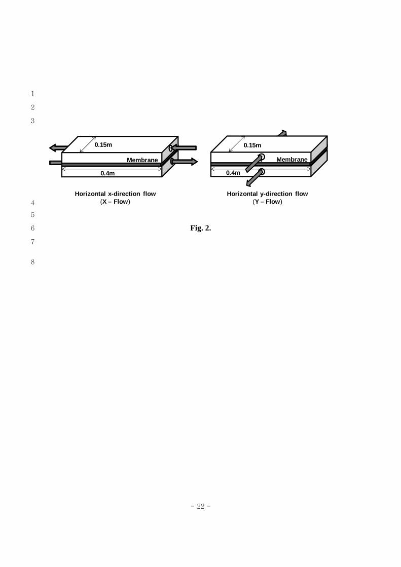
A flat-sheet module of 0.5 m length and 0.25 m width was fabricated. The membrane cell 12
consisted of two compartments, the feed side and the permeate side. The compartments were 13
made of High Density Polyethylene (HDPE) to resist corrosion by NaCl solutions and seawater. 14
The cell was designed such that the water flows occurred either along the short (Y-Flow) or long 15
(X-Flow) axis’s, and Fig. 1 shows the difference between the X-Flow and Y-Flow modes. The X-16
Flow length was 0.4 m, and Y-Flow length was 0.15 m. The flow entered and left the MD module 17
via flow distribution channels to ensure an even flow across the membrane. 18
This module design allowed the flow direction to be altered without the need to remove the 19
membrane, and it thus reduced experimental errors associated with performance differences 20
between membrane samples and handling of the membrane. 21
22
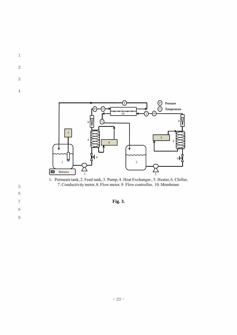
3.2 DCMD set up 23
The DCMD experimental setup is schematically depicted in Fig. 2. The module was positioned 24
horizontally so that the feed solution flowed through the bottom compartment of the cell while 25
the cooling water passed through the upper compartment. The feed and the permeate were 26
separated by a hydrophobic porous membrane, and the effective area of the membrane was 0.06 27
m2. The feed and cold solutions were contained in double walled reservoirs and circulated 28
through the membrane module using centrifugal pumps. The outlet temperatures of the hot and 29
- 7 -
cold sides were continually monitored and recorded electronically. The permeated liquid was 1
circulated through a graduated cylinder, and the volume measured at regular intervals. The purity 2
of the water extracted was determined through water conductivity using an electrical conductivity 3
meter (EC470-L, ISTEK, KOREA). 4
A series of experiments were conducted on the DCMD system to investigate the effect of flow 5
rates, flow configurations (counter-current vs. co-current), module dimensions (X-Flow vs. Y-6
Flow), salt concentration and temperature. 7
8
3.3 Membrane and membrane characteristic method 9
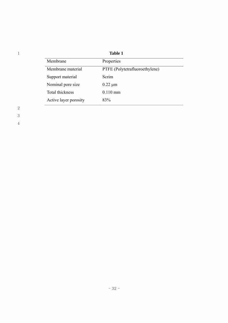
A commercially available hydrophobic porous PTFE membrane manufactured by GE 10
Osmonics (Minnesota, USA) was used for the experiments. Some of the membrane 11
characteristics provided by the manufacturer are listed in Table 1. 12
13
Liquid entry pressure (LEP) test 14
For the measurement of the LEP, the membrane was placed in a filtration cell with an effective 15
area of 0.00039 m2, and the upper portion was filled with 20% NaCl solution. The filtration cell 16
was placed in a beaker filled with pure water (Milli Q), such that the lower side of the filtration 17
cell was in contact with the pure water. Pressure was applied to the 20% NaCl solution using 18
regulated nitrogen. The pressure was increased until the NaCl solution penetrated through the 19
membrane and was mixed with the pure water in the beaker. The penetration of the NaCl through 20
the membrane was detected via a change in conductivity in the pure water by using a 21
conductivity meter. The pressure at which the NaCl solution penetrated the membrane was 22
recorded, and the average of three measurements for each of the three different samples of 23
membrane was recorded [17]. 24
25
Contact angle (CA) test 26
The CA of the membrane was measured using a SV Sigma 701 Tensiometer from KSV 27
Instruments Ltd (Helsinki, Finland). The membrane was brought into contact with a drop of pure 28
water, and the CA was calculated with the aid of the computer software. The quoted CA is the 29

- 8 -
average of the three values of CA measurements. 1
2
Scanning electron microscopy (SEM) analysis 3
The morphology of the resulting membranes was examined by scanning electron microscopy 4
(FE-SEM, Hitachi S-4800). 5
6
Gas permeability test 7
A gas permeability test was performed to verify the average pore size of the membrane. The 8
test measured the flux at various pressure drops across the membrane using a single gas 9
(nitrogen). Assuming the flow through the membrane is to be described by the Knudsen diffusion 10
- Poiseuille flow mechanism, the total mass flux can then be obtained from: 11
(10) 12
where, ε is the porosity, r is the membrane pore radius, ξ is the membrane tortuosity, δ is the 13
membrane thickness, R is the gas constant, M is the molecular weight of the gas, T is the absolute 14
temperature, η is viscosity, Pm is the average pressure within the membrane pores, and ∆P is the 15
pressure difference across the membrane. 16
The experimental was done at a constant pressure difference across the membrane (∆P = l kPa). 17
Therefore, the equation has the form: 18
N= A0 + B0·Pm 19
(11) 20
where A0 and B0 are constants [18]. 21
From Eqs. (10) and (11), the membrane pore radius r and the effective porosity ε/τ·δ can be 22
obtained from A0 and B0 by the equation: 23
(12) 24
and, 25
(13) 26
27

- 9 -
Capillary flow porometer test 1
The pore size distribution of the membrane was determined using a Capillary Flow Porometer 2
(Porous Materials, Inc., model CFP-1200-AE), which gives information about pore diameters in 3
the 0.033 – 500 μm range. The analysis was based upon a three-curve graph: dry curve, wet curve 4
and half-dry curve. The membrane was immersed overnight in a low surface tension solution of 5
porewick (16.0 dynes/cm) to ensure that the pores were fully saturated with the liquid. The 6
wetting liquid, porewick, was displaced by compressed nitrogen, and the pore size was 7
determined on the basis of the mean flow pressure when the half-dry curve intersected with the 8
wet curve. 9
10
4. Results 11
4.1 Membrane characteristics 12
The membrane characteristic results are reported in Table 2. The CA of the membrane was 13
122 ± 5° and the LEP was 160.1 ± 2.5 kPa. Both the CA and LEP results demonstrate the highly 14
hydrophobic nature of the membrane. 15
Flux N versus pressure within the pores, Pm, was plotted from the gas permeability test results. 16
Values for A0 and B0 were obtained from the intercept and slope of the straight line (Ao is the 17
intercept from equation 11 and Bo is the slope), and values of 3.08×10⁻⁴ and 1.04×10⁻⁹ were 18
obtained as per the method of [18]. The average pore diameter, 2·r, was calculated from this 19
technique using Eq. (12), and the effective porosity, ε/τ·δ, was calculated to be 17000 m-1 from 20
Eq. (13). The experiment was conducted three times, and the average membrane pore size was 21
0.28 ± 0.05 μm. 22
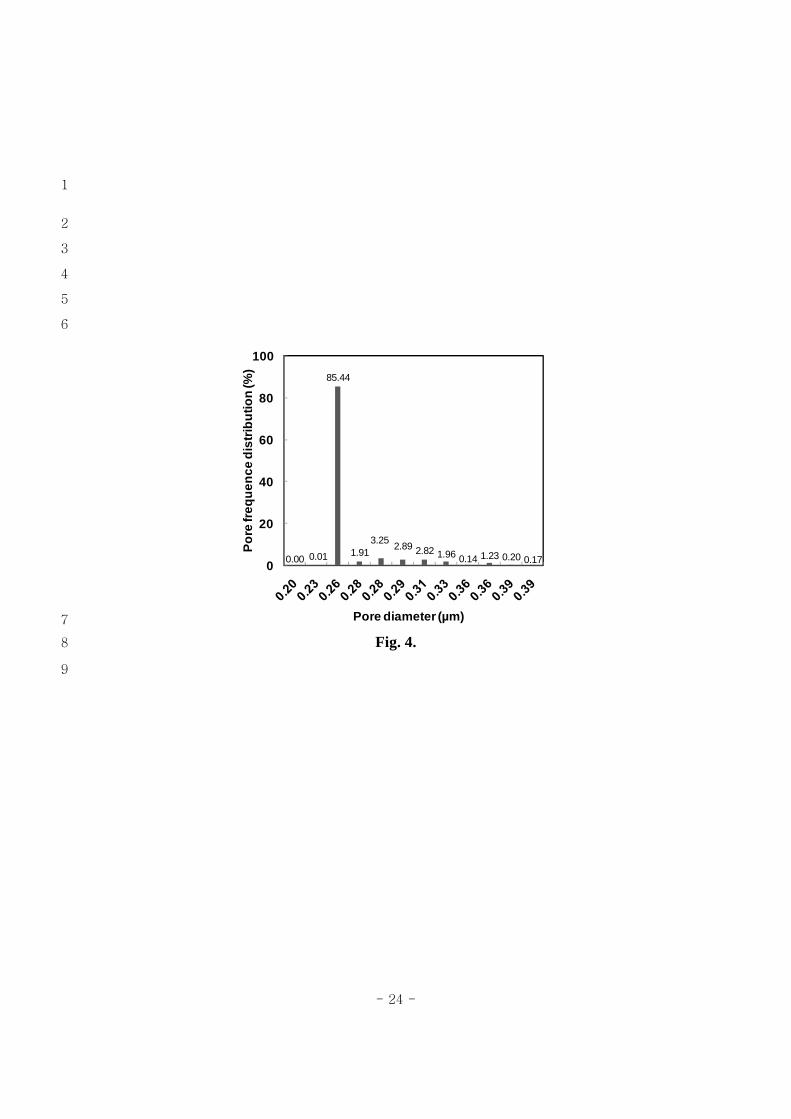
Fig. 3 shows the pore size distribution for the membrane from the capillary flow porometer 23
tests. The membrane exhibits a very narrow pore size distribution, with a mean pore size of 0.27 24
μm. The maximum pore diameter obtained from the bubble point data was 0.39 μm. This result 25
suggests that the sharp pore size distribution may minimize the potential water leakage through 26
the membrane. The pore size results obtained from the gas permeability and the capillary flow 27
porometer tests show an agreement similar to the 0.22 m value supplied by the manufacturer. 28
SEM images of the membrane surface are shown in Fig. 4 where the microstructures of the 29

- 10 -
membrane surface can be easily observed. 1
2
4.2 Effect of velocity on permeation flux and mass transfer coefficient 3
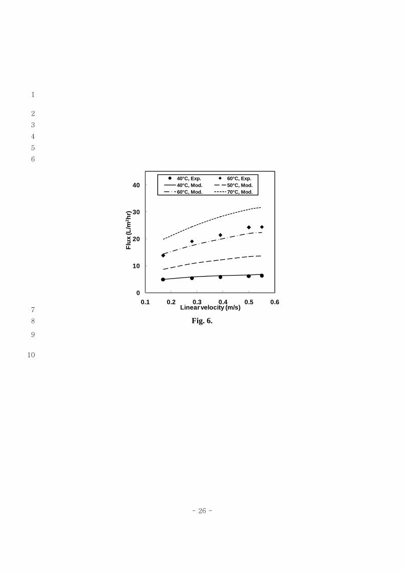
Fig. 5 shows the effect of feed velocity on the flux for both the experimental results and 4
modeling results under different feed inlet temperature conditions (NaCl concentration of 1%, 5
counter-current, and X-Flow mode). The fluxes exhibit higher values when operated at higher 6
temperature and higher velocity. It is widely understood that a temperature difference across an 7
MD membrane will induce water vapor to pass and some amount of permeate is expected to be 8
generated [19]. The flux increased with an increase in velocity from 0.17 m/s to 0.55 m/s, and it 9
seems to reach the maximum values asymptotically for high velocity. This is attributed to the 10
reduction of the boundary layer thickness when the Reynolds number increases, approaching a 11
limiting value at velocities greater than 0.50 m/s [20]. The modeling results were compared with 12
the experimental results from different velocity conditions. For lower temperature conditions, 13
modeling results show a complete agreement with the experimental results. For the higher 14
temperature curve, there was 8.6% difference between the model and experimental results when 15
the velocity was 0.50 m/s. Table 3 lists the experimental and model results for hot side and cold 16
side outlet temperatures. The modeling results show a good agreement with the experiment 17
results, with errors of less than 5.0%. The two dimension model for DCMD based on the 18
momentum, energy, and mass transfer is, therefore, accurate in its prediction of DCMD operation. 19
Fig. 6 (a) shows the effect of velocity on mass transfer coefficient for different temperature 20
conditions for the counter-current flow mode. The mass transfer coefficient increased with an 21
increase in velocity because of a reduction in temperature polarization as the flow rate and 22
Reynolds number are increased and the boundary layer thickness is reduced [18]. The 23
experimentally determined mass transfer coefficients were in the range of 0.0027 to 0.0042 24
L/m2hrPa, and they were in the range of 0.0027 to 0.0038 L/m2hrPa for the model results. The 25
values of mass transfer coefficient obtained in this study were similar to those reported by 26
Termpiyakul [21]. The values of mass transfer coefficient plateau at high velocity, irrespective of 27
the temperature, while the flux becomes constant for velocities greater than 0.50 m/s. Calculation 28
of the mass transfer coefficient compensates for the changes in temperature gradient along the 29

- 11 -
membrane, while the flux incorporates this effect into its value. Therefore, the mass transfer 1
coefficient is able to identify the fully developed conditions when the flow within the module is 2
such that temperature polarization becomes constant (0.50 m/s), while the velocities continue to 3
increase above this point because the temperature gradients along the membrane are lower and 4
hence the temperature difference and vapour pressure differences remain high [22]. This is 5
demonstrated by the temperature gradients along the membrane as shown in Fig. 6 (b). As the 6
velocity increases, the temperature profiles flatten out until there is little temperature drop along 7
the membrane (velocity higher than 0.50 m/s) and the driving force for membrane distillation 8
remains constant with further increases in velocity. 9
10
4.3 Comparison of co-current and counter-current flow mode 11
Fig. 7 shows the temperature distribution along the length of the module for co-current (a) and 12
counter-current (b) flow modes detected by the thermometers under the conditions: NaCl 13
concentration of 1%; hot side inlet temperature of 60°C, and cold side inlet temperature of 20°C, 14
and both feed and permeate side linear velocity of 0.50 m/s for X-Flow mode. The temperature 15
distribution profiles of permeate side and feed side are parallel to each other in counter-current 16
flow mode, which is different from the curves of the co-current flow mode in which the curves 17
approach each other [23]. The model simulated results were compared with the experimental 18
results, and differences of less than 3.8% were obtained, which shows good agreement between 19
the experimental and the modeling. 20
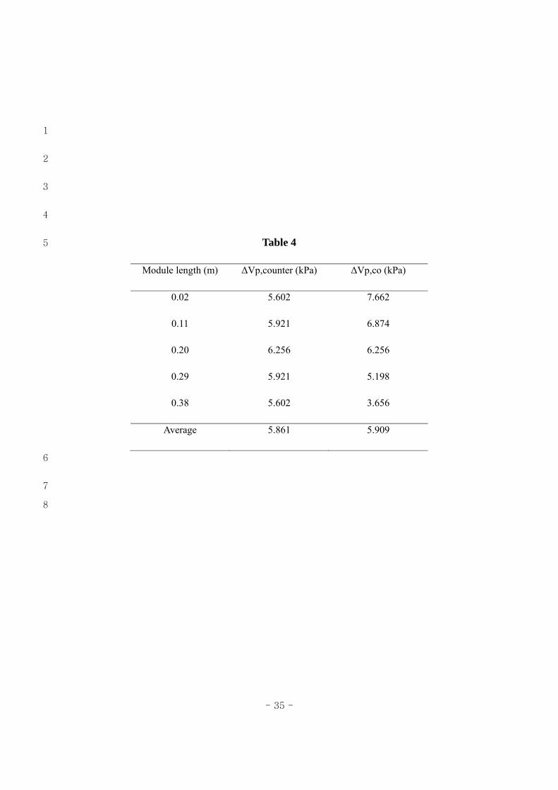
The values for vapor pressure difference for both co-current and counter-current flow modes 21
are reported in Table 4. The temperatures were converted to vapor pressures using the Antoine 22
Equation and the vapor pressure difference at each location calculated. The results indicate that 23
there was a higher vapor pressure difference in the first half of the module (0.2 m) compared to 24
the second half for the co-current mode. The vapor pressure difference for the counter current 25
mode was even in each half. However, the average vapor pressure difference for the co-current 26
and counter-current flow modes were similar. 27
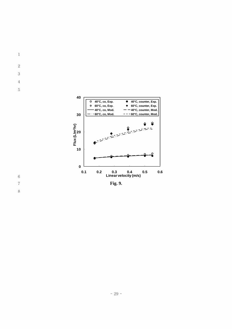
Fig. 8 compares the experimental and modeling results for the effect of velocity on flux for 28
both co-current and counter-current flow modes. The vapor pressure difference was calculated in 29

- 12 -
a manner similar to those shown in Table 4. At 40°C, the experimental results show good 1
agreement with the modeling results for both the co-current and counter-current flow modes, and 2
the fluxes for both modes were similar. However, at 60°C, the experimental results showed a 3
higher flux for the co-current mode, while the modeling results predicted the counter-current 4
mode to be a little higher. In the modeling case, the counter-current velocity is more efficient, as 5
larger trans-membrane vapor pressure was created, and this prediction agreed with our small 6
DCMD module experimental results mentioned in our previous work, and the Y-Flow mode 7
results in section 4.4. The difference cannot be distinguished since the results are well within 8
experimental error. 9
10
4.4 Comparison X-flow and Y-flow dimensions 11
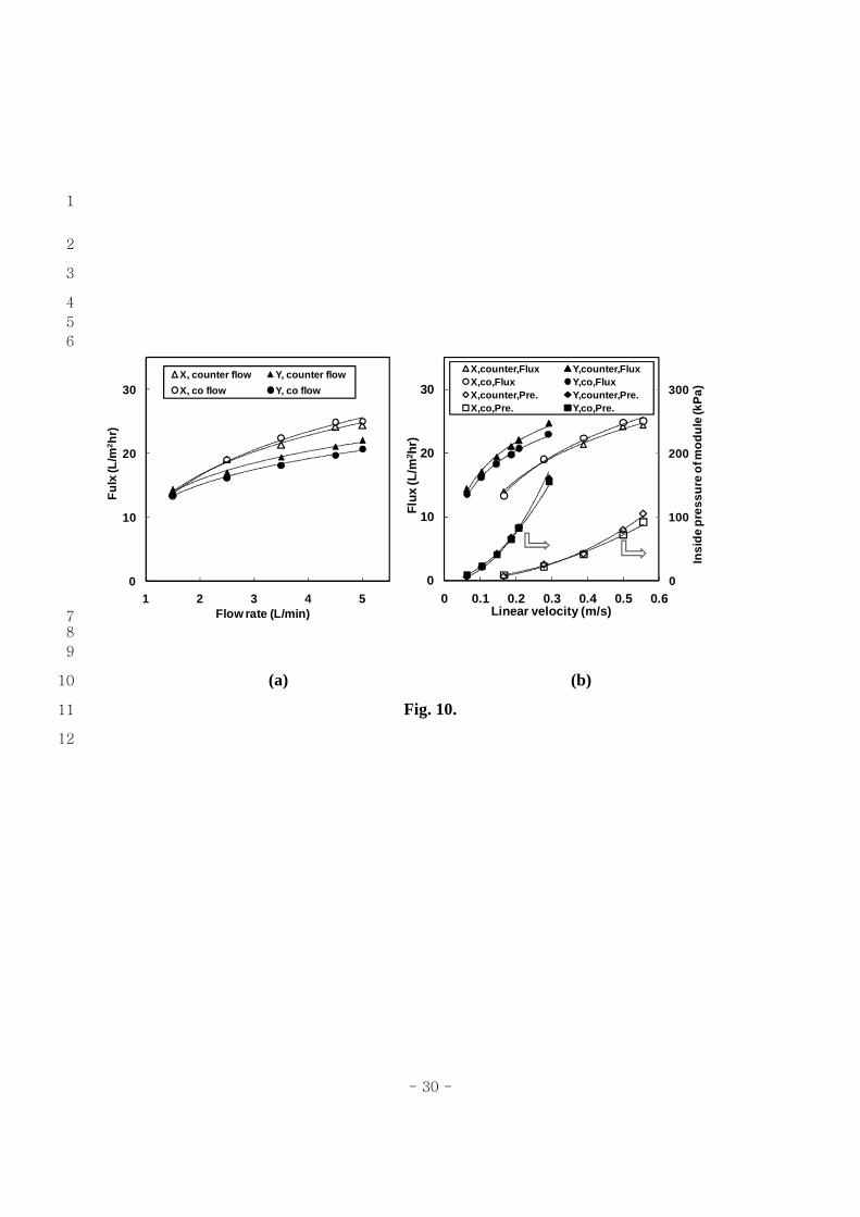
Fig. 9 (a) shows the effect of flow rate on the permeate flux for X-Flow and Y-Flow module 12
arrangements for the following conditions: NaCl concentration of 1%; hot side inlet temperature 13
of 60°C, and cold side inlet temperature of 20°C. The permeate flux increased with an increase in 14
the flow rate from 1.5 L/min to 4.5 L/min, and it seemed to reach the maximum value for flow 15
rates above 4.5 L/min in X-Flow mode for both co-current and counter-current flows. For the Y-16
Flow mode, the flux increased with an increase in the flow rate and did not reach a plateau for 17
any experimental flow rate. As stated previously, the increasing of flux with flow rate is due to 18
the reduction of the boundary layer thickness when the Reynolds number increases [17], as well 19
as the reduction in temperature gradients along the membrane. 20
Before approaching the limiting value, the X-Flow mode shows a higher flux than Y-Flow. 21
This is due to the X-Flow having a higher linear velocity under the same flow rate conditions, 22
which reduces the boundary layer thickness and increases the temperature polarization coefficient, 23
τ. This suggests that long, narrow modules are more appropriate for high flux modules than short, 24
wide modules for a given flow rate. 25
Fig. 9 (b) shows the effect of velocity on flux for both co-current and counter-current flow 26
modes for X-Flow and Y-Flow conditions. The Y-Flow mode showed a higher permeate flux for 27
both co-current and counter-current flow modes under the same linear velocity conditions 28
because the length or water path of the Y-Flow mode was shorter (0.15 m) than the X-Flow mode 29

- 13 -
(0.4 m), and, therefore, there was a lower temperature drop along the membrane for this 1
configuration. In addition, the inside pressure of the module for different velocities was also 2
observed, as shown in Fig. 9 (b). In the case of Y-Flow mode, the module’s pressure increased 3
rapidly with increasing velocity and reached 162 kPa at the velocity of 0.29 m/s. At the same 4
time, the X-Flow mode showed a gradual increase of module pressure (105 kPa) at the velocity of 5
0.56 m/s. In the case of Y-Flow, at 0.29 m/s the pressure in module had exceeded the tested 6
membrane LEP value, i.e., 160 kPa, and salt solution penetrated some parts of the membrane 7
instead of water vapor. This phenomenon resulted in an increase of the permeate conductivity 8
from 22.6 to 64.5 µS/cm within 3 hours. For the other conditions, the permeate conductivity 9
decreased with time to less than 20 µS/cm until steady state was reached, indicating that there 10
was no salt passage across the membrane for these conditions. Furthermore, high pressure can 11
lead directly to leakage problems, which would require more robust apparatus where leaks do not 12
occur. Ultimately, the desalination process was not able to continue at higher velocities for the Y-13
Flow mode. 14
As the Y-Flow mode was able to produce a higher flux at a given velocity, Fig. 9 (a) showed 15
that the X-Flow mode flux was higher for a given flow rate. Therefore, under the conditions of 16
limited membrane area and flow rate, the X-Flow mode (long skinny module) is the most 17
productive because of the reduced temperature polarization effects. The Y-Flow mode (short, 18
wide module) has the advantage of having a larger temperature difference, and hence the vapor 19
pressure difference across the membrane at any given feed velocity. However, at velocities for 20
which temperature polarization effects are reduced (i.e., above velocities for which the mass 21
transfer coefficient becomes constant), the temperature gradients along the membrane were 22
reduced and the vapor pressure differences for the X-Flow and Y-Flow modes approach each 23
other. Additionally, the long membrane length in the X-Flow mode had lower hot brine outlet 24
temperatures, and hence more thermal energy was utilized in this geometry. 25
26
4.5 Effect of NaCl concentration on permeation flux 27
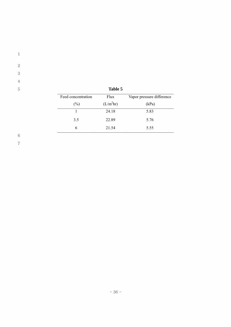
Table 5 shows the effect of salt concentration on the flux and vapor pressure difference in the 28
counter-current X-Flow mode for the conditions of a hot side temperature of 60°C, a cold side 29
- 14 -
temperature of 20°C and velocity of 0.50 m/s. The permeation flux decreased approximately 1
10.9% from 24.2 to 21.5 L/m2hr when the NaCl concentration increased from 1 to 6 wt %. The 2
vapor pressure difference decreased by approximately 4.8% from 5.83 kPa to 5.55 kPa when the 3
NaCl concentration increased from 1 to 6 wt %. The effect of salt concentration on the flux shows 4
a decrease stronger than the vapor pressure difference. The reason may be attributed to the 5
membrane surface temperature polarization, which was ignored when calculating the vapor 6
pressure difference. The polarization layers formed on either side of PTFE membrane reduce 7
water permeation in membrane distillation. This reduction is higher when the concentration 8
increases. This is the result of two opposing contributions: first, the heat transfer coefficient 9
decreased slightly with higher salt concentration, i.e., at higher salt concentration, the solution 10
viscosity becomes higher. Ultimately the thermal conductivity becomes lower, and it reduces the 11
convective heat transfer. Secondly the slower heat transfer kinetics from the bulk flow to the 12
membrane surface increases the temperature polarization. 13
14
5. Conclusions 15
DCMD experiments were performed using a PTFE membrane with a mean pore size of 0.28 16
μm and an effective porosity value of 17000 m-1. The results of the CA and LEP tests indicate 17
that the membrane is suitable for DCMD because of its high hydrophobicity. 18
The fluxes exhibit higher values when operated at higher temperature and higher velocity, and 19
they seem to reach maximum values asymptotically at high velocity. The values of mass transfer 20
coefficients observed in this study were in the range of 0.0027 to 0.0042 L/m2hrPa. 21
The temperature distribution profiles of permeate side and feed side were parallel to each other 22
in the counter-current flow mode, while the temperature profiles approach each other in the co-23
current flow. The flux and vapor pressure differences obtained for co-current and counter-current 24
values were less than 5.0%, in other words, equal to each other. 25
The permeation flux increased with an increase in the flow rate and velocity, reaching 26
maximum values asymptotically in the X-Flow mode, but there was no plateau for the Y-Flow 27
mode over the flow rate range considered in these experiments. The Y-Flow mode has the 28
advantage of having wider temperature difference at given feed velocity, but the X-Flow mode 29
- 15 -
had lower inside pressure and lower hot brine outlet temperatures, which means that more 1
thermal energy was utilized. 2
Both the flux and vapor pressure differences decreased with an increase in the NaCl 3
concentration. The effect of salt concentration on flux showed a decrease greater than the vapor 4
pressure difference, and was attributed to polarization layers formed on the membrane. 5
A two dimension model was developed through the membrane by integrating the permeate flux 6
with mass, energy and momentum balances on both feed and permeate sides. The modeling 7
results agreed well with the experimental results for different velocity and temperature conditions, 8
and both the experimental and simulation results were in accord with each other. 9
10
Acknowledgment 11
This research was conducted as part of the project by the Ministry of Commerce, Industry and 12
Energy (MOCIE) through Regional Innovation Centre (RIC). The research was partially 13
supported by a grant (07 SEAHERO B01-04-02) from the Plant Technology Advancement 14
Program funded by the Ministry of Construction & Transportation of the Korean government. 15
16
Nomenclature 17
A0 constant 18
B0 constant 19
C mass transfer coefficient 20
Cpc cold side specific heat capacity at constant pressure 21
Cph hot side specific heat capacity at constant pressure 22
Cpm specific heat capacity of the membrane at constant pressure 23
I matrix I 24
i x-direction any position i 25
J permeate flux 26
k thermal conductivity (w/m·K) 27
kc cold side liquid thermal conductivity (w/m·K) 28
- 16 -
kh hot side liquid thermal conductivity (w/m·K) 1
km liquid thermal conductivity of the membrane (w/m·K) 2
kmg liquid thermal conductivity of the membrane (w/m·K) 3
kms liquid thermal conductivity of the membrane (w/m·K) 4
L module length 5
M molecular weight of water 6
N gas flux 7
n matrix n 8
P pressure 9
P1 saturated vapor pressure on the hot side membrane surface (Pa) 10
P2 saturated vapor pressure on the cold membrane surface (Pa) 11
Pc cold side pressure (Pa) 12
Ph hot side pressure (Pa) 13
q inward heat flux (w/m2) 14
r membrane pore radius 15
R gas constant 16
T1 hot side membrane surface temperature (°C) 17
T2 cold side membrane surface temperature (°C) 18
Tc cold side temperature (°C) 19
Tc,i cold side inlet temperature (°C) 20
Tc,i cold side outlet temperature (°C) 21
Th hot side temperature (°C) 22
Th,i hot side inlet temperature (°C) 23
Th,o hot side outlet temperature (°C) 24
Tm membrane temperature (°C) 25
uc cold side flow velocity (m/s) 26
uh hot side flow velocity (m/s) 27
um flow velocity inside of membrane layer (m/s) 28
vc,i cold side inlet flow velocity (x-direction) 29
- 17 -
vh,i hot side inlet flow velocity (x-direction) 1
x x-direction 2
z z-direction 3
4
Greek letters 5
τ temperature polarization coefficient 6
ρc cold side liquid density 7
ρh hot side liquid density 8
ρm membrane density 9
ε membrane porosity 10
ξ membrane tortuosity 11
δ membrane thickness 12
η viscosity 13
14
References 15
[1] L.Carlsson, The new generation in sea water desalination SU membrane distillation system, 16
Desalination 45 (1983) 221-222. 17
[2] R. W. Schofield, A. G. Fane, C. J. D. Fell, Heat and mass transfer in membrane distillation, 18
J. Membr. Sci. 33 (1987) 299-313. 19
[3] A. M. Alklaibi, N. Lior, Membrane-distillation desalination: Status and potential, 20
Desalination 171 (2005) 111-131. 21
[4] S. Bandini, C. Gostoli, G. C. Sarti, Separation efficiency in vacuum membrane distillation, 22
J. Membr. Sci. 73 (1992) 217-229. 23
[5] L. Basini, G. D. Angelo, M. Gobbi, G.C. Sarti, C. Gostoli, A desalination process through 24
sweeping gas membrane distillation, Desalination 64 (1987) 245-257. 25
[6] M. C. García-Payo, M. A. Izquierdo-Gil, C. Fernández-Pineda, Air gap membrane 26
distillation of aqueous alcohol solutions, J. Membr. Sci. 169 (2000) 61-80. 27
[7] M. Tomaszewska, Membrane distillation-examples of applications in technology and 28
environmental protection, Environmental Studies 9 (2000) 27. 29
- 18 -
[8] G. C. Sarti, C. Gostoli, S. Bandini, Extraction of organic components from aqueous streams 1
by vacuum membrane distillation, J. Membr. Sci. 80 (1993) 21-33. 2
[9] W. T. Hanbury, T. Hodgkiess, Membrane distillation - an assessment, Desalination 56 3
(1985) 287-297. 4
[10] S. I. Andersson, N. Kjellander, B. Rodesjö, Design and field tests of a new membrane 5
distillation desalination process, Desalination 56 (1985) 345-354. 6
[11] R. Thiruvenkatachari, M. Manickam, T. O. Kwona, S. J. Kim, I. S. Moon, Separation of 7
water and nitric acid with porous hydrophobic membrane by air gap membrane distillation, 8
Separ. Sci. Technol. 41 (2006) 3187-3199. 9
[12] M. Manickam, T. O. Kwon, J. W. Kim, M. Duke, S. Gray, I. S. Moon, Effects of operating 10
parameters on permeation flux for desalination of sodium chloride solution using air gap 11
membrane distillation, Desalination and Water Treatment 13 (2010) 362-368. 12
[13] K. He, H. J. Hwang, I. S. Moon, Air gap membrane distillation (AGMD) on the different 13
types of membrane, Korean J. Chem. Eng. accepted, (2010). 14
[14] K. He, H. J. Hwang, M. W. Woo, I. S. Moon, Production of Drinking Water from Saline 15
Water by Direct Contact Membrane Distillation (DCMD), J. Ind. Eng. Chem. in press, 16 16
(2010). 17
[15] R. W. Schofield, A. G. Fane, C. J. D. Fell, Gas and vapor transport through micro-porous 18
membranes. I. Knudsen-Poiseuille transition, J. Membr. Sci. 53 (1990) 279-294. 19
[16] R. M. Felder, R. W. Rousseau, Elementary Principles of Chemical Processes, third ed., John 20
Wiley & Sons, New York, 2000. 21
[17] J. Zhang, N. Dow, M. Duke, E. Ostarcevic, J. D. Li, S. Gray, Identification of material and 22
physical features of membrane distillation membranes for high performance desalination, J. 23
Membr. Sci. 349 (2010) 295-303. 24
[18] M. S. El-Bourawi, Z. Ding, R. Ma, M. Khayet, A framework for better understanding 25
membrane distillation separation process, J. Membr. Sci. 285 (2006) 4–29. 26
[19] E. Curcio, E. Drioli, Membrane Distillation and Related Operation – A Review, Sep. Purif. 27
Rev. 34 (2005) 35 – 86. 28

- 19 -
[20] K. W. Lawson, D. R. Lloyd, Membrane distillation, J. Membr. Sci. 124 (1997) 1-2. 1
[21] P. Termpiyakul, R. Jiraratananon, S. Srisurichan, Heat and mss transfer characteristics of a 2
direct contact membrane distillation process for desalination, Desalination 177 (2005) 133-3
141. 4
[22] J. Phattaranawik, R. Jiraratananon, Direct contact membrane distillation: effect of mass 5
transfer on heat transfer, J. Membr. Sci. 188 (2001) 137-143. 6
[23] L. Martinez-Diez, F. J. Florido-Diaz, Distillation of brines by membrane distillation, 7
Desalination 137 (2001) 267-273. 8
9
10
- 20 -
Figure captions 1
Fig. 1. Schematic diagram of the simulated DCMD 2D model. (Counter-current) 2
Fig. 2. Membrane modules for X-Flow and Y-Flow modes. 3
Fig. 3. Schematic diagram of DCMD experimental setup. 4
Fig. 4. Pore size distribution of the PTFE membrane. 5
Fig. 5. SEM images of the membrane surface (a) and a higher magnified view (b). 6
Fig. 6. Experimental (Exp.) results and simulation (Mod.) results showing the effect of velocity 7
on permeate flux for different temperature conditions. (Cold side inlet temperature of 8
20°C, NaCl concentration of 1%, counter-current and X-Flow mode) 9
Fig. 7. Effect of velocity on mass transfer coefficient (a) and vapor pressure difference (b). (Cold 10
side inlet temperature of 20°C, NaCl concentration of 1%, counter-current and X-Flow 11
mode) 12
Fig. 8. Measured and predicted temperature distribution along the membrane for co-current (a) 13
and counter-current (b) flow modes. (Hot and cold side velocity of 0.50 m/s, NaCl 14
concentration of 1%, and X-Flow mode) 15
Fig. 9. Comparison of experimental and modeling results for co-current and counter-current flow 16
modes on permeate flux for different velocity conditions. (Cold side temperature of 20°C, 17
NaCl concentration of 1%, and X-Flow mode) 18
Fig. 10. Comparison different flow modes on permeate flux: (a) Effect of flow rate on permeate 19
flux; (b) Effect of linear velocity on flux and module inside pressure (Pre.). (NaCl 20
concentration of 1%; hot side inlet temperature of 60°C, and cold side inlet temperature of 21
20°C) 22
23
24
25
26
27
28
29

- 21 -
1
2
3
4
A
HG
FEDC
B
Feed channel
permeate channel
Membrane Mass
Counter-current flow mode
Th,oTh,i
Tc,o Tc,i
0
z
x
vh,i
vc,i
5
6
7
Fig. 1. 8
9
10
11
- 22 -
1
2
3
Membrane
Horizontal x-direction flow (X – Flow)
Horizontal y-direction flow (Y – Flow)
0.15m
0.4m
Membrane
0.15m
0.4m
4
5
Fig. 2. 6
7
8
- 23 -
1
2
3
4
6
Heater
Balance
P
P
T
T
T
T
8
Feed TankProduct Tank
P
T
Pressure
Temperature
5
7
Balance
P
P
T
T
T
T P
T
Pressure
Temperature
4
99
1
3
8
1 2
4
3
1. Permeate tank, 2. Feed tank, 3. Pump, 4. Heat Exchanger , 5. Heater, 6. Chiller, 7. Conductivity meter, 8. Flow meter, 9. Flow controller, 10. Membrane
10
5
6
Fig. 3. 7
8
9
- 24 -
1
2
3
4
5
6
0.00 0.01
85.44
1.913.25
2.89 2.82 1.96 0.14 1.23 0.20 0.170
20
40
60
80
100
Po
re fr
eq
ue
nc
e d
istr
ibu
tio
n (%
)
Pore diameter (µm) 7
Fig. 4. 8
9

- 25 -
1
2
3
4
5
6
7
8
Fig. 5. 9
10
- 26 -
1
2
3
4
5
6
0
10
20
30
40
0.1 0.2 0.3 0.4 0.5 0.6
Flu
x (L
/m2h
r)
Linear velocity (m/s)
40°C, Exp. 60°C, Exp.40°C, Mod. 50°C, Mod.60°C, Mod. 70°C, Mod.
7
Fig. 6. 8
9
10

- 27 -
1
2
3
4
0
0.001
0.002
0.003
0.004
0.005
0.006
0.1 0.2 0.3 0.4 0.5 0.6
Ma
ss
tra
ns
fer c
oe
ffic
ien
t (L
/m2h
rPa
)
Linear velocity (m/s)
Hot side inlet temp. 40
Hot side inlet temp. 60
0
2
4
6
8
0.1 0.2 0.3 0.4 0.5 0.6
Va
po
r pre
ss
ure
dif
fere
nc
e (k
Pa
)
L inear velocity (m/s)
Hot side inlet temp. 40
Hot side inlet temp. 60
5
6
7 ( a ) ( b ) 8
Fig. 7. 9
10

- 28 -
1
2
3
10
30
50
70
90
0 0.1 0.2 0.3 0.4
Tem
pe
ratu
re (°
C)
Membrane module length (m)
Cold side inlet temp.20 , Exp.
Hot side inlet temp.60 , Exp.
Cold side inlet temp.20 , Mod.
Hot side inlet temp.60 , Mod.
10
30
50
70
90
0 0.1 0.2 0.3 0.4
Tem
pe
ratu
re (°
C)
Membrane module length (m)
Cold side inlet temp.20 , Exp.
Hot side inlet temp.60 , Exp.
Cold side inlet temp.20 , Mod.
Hot side inlet temp.60 , Mod.
4
( a ) ( b ) 5
Fig. 8. 6
7
- 29 -
1
2
3
4
5
0
10
20
30
40
0.1 0.2 0.3 0.4 0.5 0.6
Flu
x (L
/m2h
r)
Linear velocity (m/s)
40°C, co, Exp. 40°C, counter, Exp.
60°C, co, Exp. 60°C, counter, Exp.
40°C, co, Mod. 40°C, counter, Mod.
60°C, co, Mod. 60°C, counter, Mod.
6
Fig. 9. 7
8
- 30 -
1
2
3
4
5
6
0
10
20
30
1 2 3 4 5
Fu
lx (L
/m2h
r)
Flow rate (L/min)
X, counter flow Y, counter flow
X, co flow Y, co flow
0
100
200
300
0
10
20
30
0 0.1 0.2 0.3 0.4 0.5 0.6
Ins
ide
pre
ss
ure
of m
od
ule
(kP
a)
Flu
x (L
/m2 h
r)
Linear velocity (m/s)
X,counter,Flux Y,counter,FluxX,co,Flux Y,co,FluxX,counter,Pre. Y,counter,Pre.X,co,Pre. Y,co,Pre.
7 8
9
(a) (b) 10
Fig. 10. 11
12
- 31 -
Tables 1
Table 1 Membrane characteristics provide by manufacture. 2
Table 2 Membrane characteristics from various tests. 3
Table 3 Comparison the temperature profile for both experiment result and modeling results. (Hot 4
side inlet temperature of 60°C, cold side inlet temperature of 20°C, NaCl concentration 1%, 5
counter-current, X-Flow mode) 6
Table 4 Comparison of vapor pressure difference for co-current and counter-current flow mode. 7
(Hot side inlet temperature of 60°C, cold side inlet temperature of 20°C, Hot side velocity of 0.5 8
m/s, cold side velocity of 0.5 m/s, NaCl concentration of 1%, and X-Flow mode) 9
Table 5 The effect of NaCl concentration on flux and vapor pressure difference. (Hot side inlet 10
temperature of 60°C, and cold side inlet temperature of 20°C; hot side velocity of 0.5 11
m/s, cold side veloctiy of 0.5 m/s; counter-current, X-Flow mode) 12
13
14
15
16
17
- 32 -
Table 1 1
Membrane Properties
Membrane material PTFE (Polytetrafluoroethylene)
Support material Scrim
Nominal pore size 0.22 μm
Total thickness 0.110 mm
Active layer porosity 83%
2
3
4

- 33 -
1
2
3
4
Table 2 5
Characteristics Values
LEP 160.1±2.5 kPa
Contact angle 122 ±5°
Pore size from gas permeability test 0.28±0.05 μm
Pore size from capillary flow porometry test 0.27 μm
ε/τ·δ from gas permeability test 17000 m-1
6

- 34 -
1
2
3
4
5
6
7
Table 3 8
Velocity
(m/s)
Hot outlet temp. (°C) Cold outlet temp. (°C)
Experimental Modeling Error (%) Experimental Modeling Error (%)
0.17 50.1 49.5 1.20 29.1 30.5 2.81
0.28 52.3 52.7 0.76 27.4 27.4 0.36
0.39 53.9 54.3 0.74 26.3 25.7 2.28
0.5 55.1 55.3 0.36 25.8 24.7 4.26
0.55 55.3 55.7 0.72 25.4 24.5 3.54
9
10
11
- 35 -
1
2
3
4
Table 4 5
Module length (m) ΔVp,counter (kPa) ΔVp,co (kPa)
0.02 5.602 7.662
0.11 5.921 6.874
0.20 6.256 6.256
0.29 5.921 5.198
0.38 5.602 3.656
Average 5.861 5.909
6
7
8
- 36 -
1
2
3
4
Table 5 5
Feed concentration
(%)
Flux
(L/m2hr)
Vapor pressure difference
(kPa)
1 24.18 5.83
3.5 22.89 5.76
6 21.54 5.55
6
7
Top Related