


Languages
Pages
Legal


Diploma Thesis
‐ a fine balance ‐
Modeling of Water and Mass Transport Dynamics
for an Irrigated Arid Site

TECHNISCHE UNIVERSITÄT DRESDEN
FACULTY OF FOREST, GEO AND HYDRO SCIENCES
‐ DEPARTMENT OF HYDROSCIENCES‐
Professor in charge: Prof. Dr. Peter‐Wolfgang Gräber
Supervisor: Dr. Sandra Ibañez
Granduand: Björn Helm
Matriculation number: 2924566

EIDESSTATTLICHE ERKLÄRUNG
Ich versichere, dass ich die vorliegende Diplomarbeit selbstständig verfasst und keine
anderen als die angegebenen Quellen und Hilfsmittel benutzt habe. Aus fremden Quellen
übernommene Passagen und Gedanken sind als solche kenntlich gemacht.
Diese Arbeit hat in gleicher oder ähnlicher Form noch keiner Prüfungsbehörde vorgelegen.
Dresden, den 22. Dezember 2008
Björn Helm
INDEX OF CONTENTS
1 Introduction................................................................................................................................... 1
1.1 Situation in Mendoza ......................................................................................................... 3
1.1.1 Generalities.................................................................................................................... 3
1.1.2 Climatic Conditions and Ecosystems ........................................................................ 4
1.1.3 Landscape and Hydrology.......................................................................................... 8
1.1.4 Socioeconomic Conditions ........................................................................................ 10
1.1.5 Irrigation system and silviculture ............................................................................ 10
1.2 Problems and Vulnerability related to Water Use ....................................................... 12
1.2.1 Salinization and hydro‐saline balance..................................................................... 13
1.2.2 Excess exploitation of the groundwater .................................................................. 14
1.2.3 Oil production and industry ..................................................................................... 15
1.2.4 Unmonitored reuse of waste water.......................................................................... 16
1.3 Previous Works ................................................................................................................. 17
1.3.1 State of science in water and mass transport dynamics........................................ 17
1.3.2 Projects related to agricultural water use in Mendoza.......................................... 17
1.3.3 Poplars and their interaction with the environment ............................................. 18
1.4 Model Description ............................................................................................................ 20
1.4.1 Physical base of flow and mass transport ............................................................... 21
1.4.2 Numerical solution of the governing equations .................................................... 28
1.4.3 Input data .................................................................................................................... 29
1.4.4 Limits and possibilities .............................................................................................. 30

2 Material and Methods................................................................................................................ 31
2.1 Investigated site................................................................................................................. 31
2.1.1 Environmental Conditions at the site ...................................................................... 32
2.2 Situation and Data at the site........................................................................................... 35
2.2.1 Previous projects......................................................................................................... 35
2.2.2 Sample taking.............................................................................................................. 36
2.2.3 Available Data............................................................................................................. 37
2.2.4 Preprocessing .............................................................................................................. 38
2.2.5 Completion and Regionalization of climate data................................................... 39
2.2.6 Roots and water uptake............................................................................................. 41
2.2.7 Actual transpiration of the trees............................................................................... 42
2.3 Soil properties.................................................................................................................... 43
2.3.1 Physical soil properties .............................................................................................. 44
2.3.2 Water Dynamics ......................................................................................................... 44
2.3.3 Mass Transport ........................................................................................................... 48
2.4 Modeling ............................................................................................................................ 49
2.4.1 Conceptual Model ...................................................................................................... 49
2.4.2 Model Setup ................................................................................................................ 51
2.5 Representation of present state ....................................................................................... 53
2.5.1 Sensitivity analysis ..................................................................................................... 53
2.5.2 Calibration and Validation........................................................................................ 54
2.6 Scenario Setup ................................................................................................................... 58
2.6.1 Salinization due to irrigation .................................................................................... 58
2.6.2 Irrigation with alternative irrigation methods ....................................................... 59
2.6.3 Phytoremediation of petroleum contamination..................................................... 60
3 Results and Discussion .............................................................................................................. 64
3.1 Processing and evaluation of input data ....................................................................... 64
3.1.1 Climate data and plant data...................................................................................... 64
3.1.2 Soil data analysis ........................................................................................................ 72
3.1.3 Estimation of soil hydraulic and transport parameters ........................................ 87
3.2 Sensitivity Analysis........................................................................................................... 94
3.3 Calibration and Validation .............................................................................................. 97
3.3.1 Calibration parameters and model performance................................................... 97
3.4 Modeling results.............................................................................................................. 105
3.4.1 Numerical stability and mass balance ................................................................... 105
3.4.2 Heterogeneity of soil moisture distribution ......................................................... 106
3.4.3 Groundwater recharge and salt balance ............................................................... 108
3.5 Scenarios Analysis .......................................................................................................... 110
3.5.1 Salinization and irrigation with alternative methods ......................................... 110
3.5.2 Phytoremediation of petroleum contamination................................................... 114
4 Conclusions ............................................................................................................................... 116
4.1 Limitations ....................................................................................................................... 116
4.1.1 Data base.................................................................................................................... 116
4.1.2 Modeling.................................................................................................................... 117

4.1.3 Scenarios .................................................................................................................... 119
4.2 Findings............................................................................................................................ 119
4.2.1 Treatment and assessment of input data .............................................................. 119
4.2.2 Model performance .................................................................................................. 120
4.2.3 Model Verification for an Arid Climate ................................................................ 120
4.2.4 Water Balance of Poplars......................................................................................... 121
4.2.5 Scenarios and Best Management Recommendations .......................................... 121
4.3 Outlook............................................................................................................................. 122
4.3.1 Data situation ............................................................................................................ 122
4.3.2 Suggestions for model development ..................................................................... 122
4.3.3 Possible continuation ............................................................................................... 123
5 Quellenverzeichnis................................................................................................................... 125

INDEX OF FIGURES
Fig. 1 Extension of the oasis in Mendoza province [Abraham, 1999] ........................................... 4
Fig. 2 Aridity index (l) and annual precipitation (r) for Mendoza province [Roig, 1999].......... 5
Fig. 3 Annual course of temperatures for Mendoza observatory climate station ....................... 6
Fig. 4 Annual courses of sunshine duration (d_sol), wind speed (u), precipitation and relative
air humidity (rh) for Mendoza observatory climate station.............................................. 7
Fig. 5 Monthly mean discharge of Río Mendoza at Estación Guido [DGI, 2007a]...................... 8
Fig. 6 Portions of water sources in irrigation for Río Mendoza (left) and Tunuyán Inferior
(right)....................................................................................................................................... 11
Fig. 7 Water content, relative saturation and relative permeability for a model loam............. 24
Fig. 8 Course of the water uptake scaling function a(h), estimate for poplars .......................... 26
Fig. 9 Satellite image of the investigated site (from: google earth virtual globe program)...... 31
Fig. 10 Map of soils according to soil genesis in the department of Rivadavia [MdR; 2008] .. 32
Fig. 11 Natural vegetation in the surrounding of the investigated site...................................... 34
Fig. 12 Schematization of the investigated site during irrigation – plant growth project........ 35
Fig. 13 Distribution of sample points at the site ............................................................................ 36
Fig. 14 Configuration of sample points (MP = measurement point) ........................................... 37
Fig. 15 Position of climate stations and investigation site in the northern part of Mendoza
province .................................................................................................................................. 39
Fig. 16 Change of concentration course due to hydromechanic dispersion .............................. 47
Fig. 17 Scheme of relevant processes of water and mass transport dynamics in SiWaPro ..... 50
Fig. 18 Accumulated evapotransiration rates and fitted trends .................................................. 65
Fig. 19 Correlation between mean temperature and average temperature at San Martin CS. 66
Fig. 20 Correlation between evaporation from San Martin and La Libertad............................. 67
Fig. 21 Courses of evaporation and precipitation from San Martin and La Libertad............... 68
Fig. 22 Measured, calculated and interpolated courses of evaporation ..................................... 69
Fig. 23Actual evapotranspiration and crop coefficients for six year poplars ............................ 72
Fig. 24 Georeferenced distribution of sample points .................................................................... 73
Fig. 25 Grain size distribution of six soils at the investigation site ............................................. 77
Fig. 26 Correlation between texture class portion and sedimentation volume......................... 78
Fig. 27 Position of the cross sections (lines) for the interpolation of soil properties................. 79
Fig. 28 Distribution of sedimentation volumes within the four sampling layers ..................... 80
Fig. 29 Distribution of sedimentation volumes along three cross sections ................................ 81
Fig. 30 Measured retention curves and comparison to estimation models ............................... 82
Fig. 31 Measured and fitted curve progression for concentration breakthrough of two soils 83
Fig. 32 Estimation of retention properties with ROSETTA model and measured values for
sample 2.4 ............................................................................................................................... 88
Fig. 33 Estimation of retention properties with DIN 4220 parameter sets for sample 2.4 ....... 89
Fig. 34 Measured and fitted retention curves................................................................................. 91
Fig. 35 Unsaturated hydraulic conductivities as a function of water tension head.................. 92
Fig. 36 Discharge courses for different hydraulic conductivities ................................................ 95
Fig. 37 Sensitivities of water content to van‐Genuchten parameters .......................................... 96
Fig. 38 Calibration performance for water contents at 15 cm and 120 cm depth ...................... 99
Fig. 39 Quality assessment of a calibration version..................................................................... 100
Fig. 40 Performance utilities for an virtual optimum model, calibration and validation cases
................................................................................................................................................ 105
Fig. 41 Spatially heterogeneous distribution of soil humidity during an irrigation pulse .... 106
Fig. 42 Percolation at the lower model boundary, under a plant and between plants........... 107
Fig. 43 Distribution of NaCl concentration at a plant (x=6m) and between two stands (x=8m)
................................................................................................................................................ 111
Fig. 44 Drainage water salt concentration and accumulated load at lower boundary........... 112
Fig. 45 Concentrations and loads for benzene scenario alternatives. ....................................... 114

INDEX OF TABLES
Tab. 1 Soil properties at La Libertad................................................................................................ 33
Tab. 2 Climate characteristics at La Libertad.................................................................................. 34
Tab. 3 Plausibility ranges of measured parameters...................................................................... 38
Tab. 4 Properties of the climate stations considered for Evaporation calculation .................... 39
Tab. 5 Parameters on root water uptake for deciduous trees....................................................... 42
Tab. 6 Levels of data requirements and modelling objective....................................................... 49
Tab. 7 Assumptions for benzene transport scenarios.................................................................... 62
Tab. 8 Mass transport parameters for the benzene transport scenarios ..................................... 63
Tab. 9 Mean evaporation rates during irrigation seasons ............................................................ 65
Tab. 10 Coefficients of determination for the correlation of precipitation depths.................... 70
Tab. 11 Actual water consumption (transpiration) from different soil depths ......................... 71
Tab. 12 Bulk densities at different sample points and sample layers ................................... 74
Tab. 13 Particle densities at different sample points and sample layers.............................. 74
Tab. 14 Soil porosities at different sample points and sample layers and according to
different determination methods ........................................................................................ 75
Tab. 15 Sedimentation volumes at different sample points and sample layers .................. 76
Tab. 16 Texture porperties and classification for sampled soils .................................................. 78
Tab. 17 Saturated hydraulic conductivity of four soil samples .................................................... 83
Tab. 18 Qualitative retention parameters and ranks for seven day irrigation .................... 84
Tab. 19 Clay content values at different sample points and sample layers ......................... 86
Tab. 20 Organic matter contents at different sample points and sample layers ................. 86
Tab. 21 pH values at different sample points and sample layers.......................................... 87
Tab. 22 RETC estimates of van Genuchten parameters and statistical analysis........................ 89
Tab. 23 Unsaturated hydraulic conductivity parameters, ROSETTA estimate ......................... 93
Tab. 24 Probability quantiles for van Genuchten parameters...................................................... 94
Tab. 25 Sensitivity indexes for the different soil parameters and target variables ................... 96
Tab. 26 Parameters addressed during the calibration................................................................... 97

Tab. 27 Fitting quality parameters of calibration and validation .............................................. 101
Tab. 28 utility function thresholds and weighting coefficients for performance utility analysis
................................................................................................................................................ 104
Tab. 29 Water balance and balance based salt load..................................................................... 110
Tab. 30 Water balance and modelled salt load............................................................................. 113

ABBREVIATIONS
ACRE..................... ...............................................................area de cultivos restringidos especiales
BTEX………........................................................................... benzene, toluol, ethylbenzene, xylene
CdC…………............................................................................................................. Chacras de Coria
CDE................................................................................................. Convection‐Dispersion‐Equation
CS…………….. ...............................................................................................................climate station
DGI....................... .................................................................... Departamento General de Irrigación
EC….......................................................................................................................electric conductivity
ET…..................... ....................................................................................................evapotranspiration
IDW…………………................................................................................ inverse distance weighting
INTA.......................................................................Instituto Nacional de Tecnología Agropecuaria
kc………… ................................................................................................................. crop coefficient
LL………………. .................................................................................................................La Libertad
MA………….. ............................................................................................................Mendoza Airport
m asl...................................................................................................................meters above sea level
m bsl..................... ......................................................................................meters below surface level
MO………….......................................................................................................Menoza Observatory
MReg………. .........................................................................................................multiple regression
ND…………...........................................................................................................normal distribution
PAH………... .......................................................................................... polyaromatic hydrocarbons
PHC………….. .............................................................................................petroleum hydrocarbons
PM…………..............................................................................................................Penman Monteith
PTF..................... .................................................................................................pedotransfer function
PWP…………. .............................................................................................. permanent wilting point
R…………….. .................................................................................................... correlation coefficient
PP…………….................................................................................................performance parameter
PU………….. ......................................................................................................... performance utility
PV…………....................................................................................................................porous volume
R²……………...........................................................................................coefficient of determination
rH / rh..................... ....................................................................................................relative humidity
RMSE………....................................................................................................root mean square error
rRMSE..................... ...........................................................................relative root mean square error
SD.............................................................................................................................standard deviation

SV..................... ..................................................................................................sedimentation volume
SM……………......................................................................................................................San Martín
VC..................... ..................................................................................................... variation coefficient
WC..................... ...............................................................................................................water column
INDEX OF SYMBOLS AND UNITS
a(h) root water uptake scaling function ........................................................................... [‐]
awc available water capacity.................................................................................. [‐], L, [%]
b(x,z) water uptake distribution function ........................................................................... [‐]
Cx coefficient of friction...................................................................................................M‐²
d_sol sunshine duration..........................................................................................................T
DB bulk density ..............................................................................................................M/L³
DP particle density ........................................................................................................M/L³
ea actual vapour pressure .....................................................................................M/(LT²)
EC electric conductivity… ...................................................................................(I²T³/ML³)
ECe soil salinity.......................................................................................................(I²T³/ML³)
es saturation vapour pressure ..............................................................................M/(LT²)
ET0 Potential evapotranspiration…................................................................................ L/T
fc field capacity .................................................................................................... [‐], L, [%]
g acceleration of gravity .............................................................................................L/T²
h water pressure / suction head ......................................................................................L
h1‐h4 characteristic pressure heads of root uptake function..............................................L
)h(k unsaturated hydraulic conductivity ...................................................................... L/T
Kij components of a dimensionless anisotropy tensor ................................................ [‐]
kx coefficient of permeability in direction of x .......................................................... L/T
Ls transpiration active surface width ..............................................................................L
m transformation parameter .......................................................................................... [‐]
n increase parameter ...................................................................................................... [‐]
p pressure ....................................................................................................................M/L²
P Precipitation ............................................................................................................... L/T
pc capillary pressure head ..........................................................................................M/L²
pwp permanent wilting point...................................................................... [‐], L, [%], M/L²
rH relative humidity ............................................................................................L³/L³ = [‐]
Rn net radiation at the crop surface ............................................................................. L/T
s slope of the vapour pressure curve............................................................... M/(LT²θ)
Se relative/effective saturation............................................................................L³/L³ = [‐]
SV sedimentation volume ............................................................................................L³/M
T/Tm mean daily air temperature at 2 m height .................................................................θ

Tmin/max minimum/maximum daily air temperature at 2 m height .....................................θ
TP potential transpiration rate....................................................................................... L/T
u2 wind speed at 2 m height ........................................................................................ L/T
vx velocity of flow in direction of x ............................................................................. L/T
w0 source/sink term........................................................................................................L³/T
w0(h) actual water uptake rate ..........................................................................................L³/T
wc volumetric water content .................................................................................L³/L³, [‐]
wP potential water uptake rate .....................................................................................L³/T
α scaling parameter......................................................................................................... [‐]
η dynamic viscosity .................................................................................................M²/LT
φ porosity .............................................................................................................L³/L³ = [‐]
λ tortuosity parameter.................................................................................................... [‐]
ρ density of the fluid .................................................................................................M/L³
θ water content....................................................................................................L³/L³ = [‐]
sθ saturated water content .........................................................................................L³/L³
rθ residual water content ............................................................................................L³/L³
γ psychrometric constant..................................................................................M/(L*T²θ)
ABSTRACT
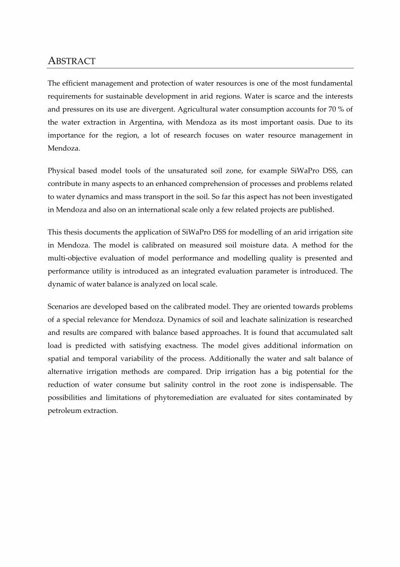
The efficient management and protection of water resources is one of the most fundamental
requirements for sustainable development in arid regions. Water is scarce and the interests
and pressures on its use are divergent. Agricultural water consumption accounts for 70 % of
the water extraction in Argentina, with Mendoza as its most important oasis. Due to its
importance for the region, a lot of research focuses on water resource management in
Mendoza.
Physical based model tools of the unsaturated soil zone, for example SiWaPro DSS, can
contribute in many aspects to an enhanced comprehension of processes and problems related
to water dynamics and mass transport in the soil. So far this aspect has not been investigated
in Mendoza and also on an international scale only a few related projects are published.
This thesis documents the application of SiWaPro DSS for modelling of an arid irrigation site
in Mendoza. The model is calibrated on measured soil moisture data. A method for the
multi‐objective evaluation of model performance and modelling quality is presented and
performance utility is introduced as an integrated evaluation parameter is introduced. The
dynamic of water balance is analyzed on local scale.
Scenarios are developed based on the calibrated model. They are oriented towards problems
of a special relevance for Mendoza. Dynamics of soil and leachate salinization is researched
and results are compared with balance based approaches. It is found that accumulated salt
load is predicted with satisfying exactness. The model gives additional information on
spatial and temporal variability of the process. Additionally the water and salt balance of
alternative irrigation methods are compared. Drip irrigation has a big potential for the
reduction of water consume but salinity control in the root zone is indispensable. The
possibilities and limitations of phytoremediation are evaluated for sites contaminated by
petroleum extraction.

KURZFASSUNG
Die effiziente Nutzung und der Schutz von Wasserressourcen ist eine der grundlegendsten
Anforderungen an die nachhaltige Entwicklung in ariden Gebieten. Wasser ist knapp und
die Interessen und Belastungen für seine Nutzung divergieren. Wasserverbrauch in der
Landwirtschaft hat einen Anteil von 70 % an der argentinischen Wassergewinnung zur
Nutzung und Mendoza ist die wichtigste Oase des Landes. Auf Grund der Wichtigkeit des
Themas für die Region ist die Erforschung der Wasserressourcen ein
Forschungsschwerpunkt in Mendoza.
Die physikalisch basierte Modellierung der ungesättigten Bodenzone, zum Beispiel mit
SiWaPro DSS kann in vielen Bereichen zu einem verbesserten Verständnis von Prozessen
und Problemen des Bodenwasser‐ und ‐stoffhaushaltes beitragen. Bislang wurden zu diesem
Thema in Mendoza noch keine Untersuchungen durchgeführt und auch international ist nur
eine kleine Zahl von Untersuchungen aus ariden Schwellenländern veröffentlicht.
Die vorliegende Arbeit dokumentiert die Anwendung von SiWaPro DSS für die
Modellierung eines ariden Bewässerungsstandortes in Mendoza. Das Modell wird auf der
Basis gemessener Bodenfeuchtedaten kalibriert. Es wird ein Verfahren zur multikriteriellen
Bewertung des Modellverhaltens und der Modelgüte vorgestellt und der Performanz‐
Nutzwert als integraler Bewertungsparameter eingeführt. Die Dynamik des
Wasserhaushaltes wird auf lokaler Skale analysiert.
Auf Basis des kalibrierten Modells werden Szenarien entwickelt die für Mendoza besonders
relevante Probleme behandeln. Die Dynamik der Versalzung des von Boden und
Sickerwasser wird untersucht und die Ergebnisse mit bilanzierenden Ansätzen verglichen.
Dabei zeigt sich dass die Bilanzansätze eine gute Voraussagegenauigkeit für die
akkumulierte Salzfracht treffen, durch die Modellierung können aber zusätzliche Aussagen
zur räumlichen und zeitlichen Variabilität der Prozesse getroffen werden. Zusätzlich wird
der Wasser‐ und Salzhaushalt für alternative Bewässerungsmethoden untersucht und mit
den zuvor gewonnen Ergebnissen verglichen. Das Potential zur Wassereinsparung durch
Tröpfchenbewässerung ist groß, allerdings ist eine Steuerung der Salzkonzentration in der
Wurzelzone unabdingbar. Des Weiteren werden die Möglichkeiten und Grenzen der
Anwendung von Phytoremediation für die in Mendoza vorkommenden Altlasten der
Erdölförderung bewertet.

RESUMEN
El uso eficiente del agua y la protección de los recursos hídricos son unos de los
requerimientos más fundamentales para el desarrollo sostenible en ámbitos áridos. La
disponibilidad de agua es limitada e intereses y presiones para su uso son divergente. La
agricultura contribuye con un 70 % al total de las extracciones para el uso del agua. Mendoza
es el oasis mas importante de la Argentina. Debido a la importancia del tema para la región,
la investigación de los recursos de agua representa un tema central en la agenda científica de
Mendoza.
La modelización de base física de la zona no saturada del suelo, por ejemplo con el programa
de simulación SiWaPro DSS es apta para mejorar el conocimiento de procesos y problemas
de los balances de agua y substancias en el suelo. Hasta ahora no hay investigaciones sobre
este tema en Mendoza y además a la escala global pocos proyectos están publicados desde
países emergentes con condiciones áridas.
Esta tesis documenta la aplicación del programa SiWaPro DSS para la modelización de un
sitio de regadío árido en Mendoza. El modelo fue calibrado en base a contenidos de
humedades medidas del suelo. Un método para la evaluación multi‐objetiva es presentado.
El parámetro de rendimiento de utilidad (performance utility) es introducido. La dinámica
del balance de agua es analizada a escala local
A partir del modelo calibrado, escenarios que tratan problemas relevantes de Mendoza son
desarrollados. La dinámica de salinización del suelo y del agua de drenaje es determinada y
comparada con un método de balance. Este método muestra una buena capacidad predictiva
para la carga acumulada de sales, adicionalmente el modelo de simulación da informaciones
sobre la variación temporal y espacial de los procesos determinates. El balance hídro‐salino
también es revisado para métodos de riego alternativos. El riego por goteo tiene gran
capacidad para el ahorro de agua pero un control de la salinización en la rizosfera es
indispensable. Además las posibilidades y limitaciones para la aplicación de la
fitoremediación con álamos para sitio contaminado con hidrocarburos petroleros son
evaluadas.

1
1 INTRODUCTION
The understanding and control of soil water dynamics is crucial in irrigated sites of arid
regions. On the one hand water is sparse and only its effective use permits a sustainable
development. On the other hand, due to the accelerated climatic driving forces and a soil
water balance strongly actuated by evaporation, mismanagement of irrigation systems may
lead to rapid loss of their full functionality e.g. caused by salinization.
Within the last four decades the advances in water related process comprehension and
computing power opened a new basis for the representation and evaluation of water
management practices. In the context of integrated land and water resources management
[Calder, 2005] calls the opportunities of model application for an enhanced understanding of
water systems and decision support the “blue revolution” that consequential widens the
view from structural engineering tasks to system oriented management strategies.
Coupling different sub‐systems is not a straight forward task. Processes are driven on
different temporal and spatial scales. Water in the distribution channels and on the field
surface flows rapidly: velocity accounts with meters per second and traveling time is usually
limited to some hours. The water in the unsaturated zone moves with centimeters or
millimeters per hour while storage time is up to some weeks. Finally groundwater moves
even slower and travel times may reach various years [Dyck, 1995]. Accounting for the
spatial extensions surface flow may be captured one dimensionally with several kilometers
of lateral movement in contrast to a few meter of cross sectional dimension. Water
movement in the unsaturated zone takes place mostly vertically and is often represented
sufficiently with two dimensional approaches, yet heterogeneously for differing soil or
cultivation situations. The aquifer demands representation for both horizontal and vertical
flow, processes and parameters are often connected and related within large spatial extends
[Schmitz, 2007], [Dogan, 2005]. The varying spatial and temporal scales and dimensions
cause difficulties for defining sensible observation boundaries that cover all three processes.
Between the highly dynamic surface flow and large scale groundwater movement,
unsaturated zone acts as an agent [Benson, 2007]. Hence special attention should be drawn
on the representation of the processes there.
Unsaturated flow is a highly non‐linear process, which complicates analysis of reactions of
the vadose zone. Consequently, engineers traditionally have used simplified solutions for
analysis of unsaturated flow problems [Benson, 2007]. For physical based two dimensional

2
(2D) modelling of water dynamics in the unsaturated zone few references are available for
arid zones although it serves as handy tool. Some work is done in one dimensional (1D)
physical based modelling, compare [Dixon, 1999], [Keese, 2005] or with conceptual models
[Querner, 2008], [Hsieh, 2001]. [Kavazanjian, 2006] points out the difficulties with modelling
the unsaturated soil layer in arid regions.
Root dynamics and soil water models are available for operation on different scales but
results for the scale transition are often not consistent [Li, 2006], [Feddes, 2001]. Dynamically
coupled models of soil water and root dynamics, e. g. [Hopmans, 1998] are still under
development, especially due to a lag of sufficiently resolved data. In order to enhance system
comprehension and to validate existing approaches on regional scale as e. g. of [Querner,
2008] it is valuable to consider processes of the unsaturated soil zone at site‐scale.
Mendoza is situated in the western part of central Argentina. The environment of the
province consists of a desert plain with precipitation about 200 mm/a and the Andes
mountain range with important glacial water recourses. The water flows from the mountain
range in rivers and is used in elaborate irrigation systems. Oases cover 3 % of Mendoza’s
province surface [Chambouleyron, 1990] and constitue the most important irrigation region
of Latin America [Peyke, 1998]. The cultivation of wine and fruit dominates the agricultural
production in Mendoza but, given the increasing demand for wood and biomass
[Bustamante, 2008], silviculture constantly gains importance in the cultivation schemes.
Mendoza’s irrigation system is one of the most sophisticated in Latin America
[Chambouleyron, 1990]. With the expansion of irrigated surface, groundwater is used
increasingly for irrigation purposes [Kupper, 2002]. The intensified use causes increased
attention for this recourse. As a result various projects are carried out to monitor and
evaluate the development, e.g. [Ortíz, 2005], [Mastrantonio, 2006]. Considering projects in
Mendoza that focus modelling the water dynamics of agricultural areas [Querner, 2008] has
done the probably most integral work.
In the present work, a model was set up to reproduce irrigation and groundwater recharge.
As study area a site was chosen that was investigated in a former study about the irrigation
of poplars. From the former works detailed climate, soil and water dynamics data were
available. It was calibrated with soil moisture data applying a set of multiple performance
parameters. The model is validated with irrigation seasons and irrigation regimes other than
the calibration data. Based on the calibrated model of water dynamics, mass transport
3
scenarios were applied that comprise some of the environmental problems related to water
use in Mendoza region.
One intention of this work is to validate the applicability of SiWaPro, a 2D model of flow
dynamics and mass transport in the unsaturated soil zone, under arid conditions. The
present work aims to give an example for the dynamics of groundwater recharge on the local
scale. It permits the validation of estimates on larger scale and gives an insight into the small
scale heterogeneity of the process dynamics.
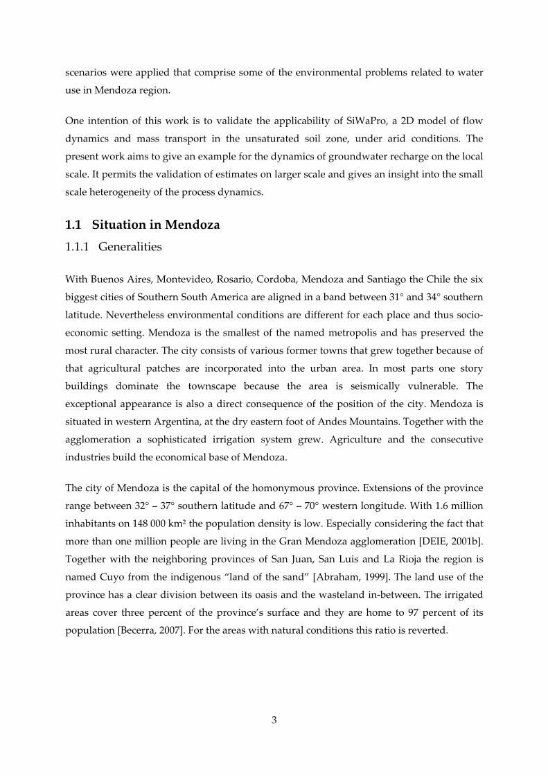
1.1 Situation in Mendoza 1.1.1 Generalities
With Buenos Aires, Montevideo, Rosario, Cordoba, Mendoza and Santiago the Chile the six
biggest cities of Southern South America are aligned in a band between 31° and 34° southern
latitude. Nevertheless environmental conditions are different for each place and thus socio‐
economic setting. Mendoza is the smallest of the named metropolis and has preserved the
most rural character. The city consists of various former towns that grew together because of
that agricultural patches are incorporated into the urban area. In most parts one story
buildings dominate the townscape because the area is seismically vulnerable. The
exceptional appearance is also a direct consequence of the position of the city. Mendoza is
situated in western Argentina, at the dry eastern foot of Andes Mountains. Together with the
agglomeration a sophisticated irrigation system grew. Agriculture and the consecutive
industries build the economical base of Mendoza.
The city of Mendoza is the capital of the homonymous province. Extensions of the province
range between 32° – 37° southern latitude and 67° – 70° western longitude. With 1.6 million
inhabitants on 148 000 km² the population density is low. Especially considering the fact that
more than one million people are living in the Gran Mendoza agglomeration [DEIE, 2001b].
Together with the neighboring provinces of San Juan, San Luis and La Rioja the region is
named Cuyo from the indigenous “land of the sand” [Abraham, 1999]. The land use of the
province has a clear division between its oasis and the wasteland in‐between. The irrigated
areas cover three percent of the province’s surface and they are home to 97 percent of its
population [Becerra, 2007]. For the areas with natural conditions this ratio is reverted.

Fig. 1 Extension of the oasis in Mendoza province [Abraham, 1999]
1.1.2 Climatic Conditions and Ecosystems
Due to the geographic location of the region, Mendoza is exposed to an arid climate. The
leeward position of the province on the foothill of the Andes causes regularly dry
atmospheric conditions. Especially during the southern hemisphere winter months (June –
August) when Intertropical Convergence Zone shifts northwards, Mendoza lies in a
subtropical trade wind zone [Schneider, 1998], as a consequence winter is the driest season.
4

Fig. 2 Aridity index (l) and annual precipitation (r) for Mendoza province [Roig, 1999]
Annual precipitation in the desert plain is about 200 mm, rising with increasing altitude but
also with distance to the mountain chain westward (Fig. 2), as the leeward influence
decreases. Driest areas are found in the Northwestern part of the province. At climate station
(CS) “El Retamo” in the North of Mendoza an annual mean precipitation of 81 mm was
registered. Highest Precipitation occurs in the main mountain range. Aridity index expresses
the ration of annual potential evaporation to annual precipitation, for values smaller than
one precipitation does not cover the evaporation demand, for values smaller than 0.5 climate
is considered as semi‐arid, for values as low as 0.03 (30 times less precipitation than potential
evaporation) climate is hyperarid. Fig. 2 displays the aridity index for Mendoza province.
Apart from the mountain range and the westernmost zones the climate is semiarid to arid.
According to Köppen/Geiger climate is desertic cold (BWk), according to Troll subtropical
arid (IV.5) or corresponding to Lauer subtropical continental arid (B.2a).
All numbers in Fig. 3 and Fig. 4 are based on a reference period of 1990 – 2005. In Fig. 3
temperature courses for Mendoza observatory are displayed. The hottest months are
December and January with a temperature of 23°C average. The coldest month is July with
an average of 7°C. Differences between minimum, mean and maximum daily temperature
5

are quite constant throughout the year and amount around seven degrees constantly. The big
differences between highest and lowest daily temperatures can be explained with the arid
surrounding, where only small water resources in soil and surface buffer the radiation heat
fluxes.
0
15
30
45
1 4 7 10month
T [°C]
Tm Tmax Tmin
Fig. 3 Annual course of temperatures for Mendoza observatory climate station
The course of hydrometeorologic parameters relative humidity (rh), precipitation (P) and
potential evapotranspiration (ETP) as well as sunshine duration (d_sol) and wind speed (u)
two meters above ground are given in Fig. 4. Precipitation is highest in the summer months
January to March. Annual precipitation is 230 mm. Relative air humidity varies between 50
and 60 % and tends to be higher in the autumn and the winter months. Sunshine duration,
wind speed and evaporation show unimodal distribution all with highest values in summer.
For all these effects elevated solar radiation in summer can be seen in a more or less direct
relation as driving force.
6

0
50
100
150
200
1 3 5 7 9 11month
ETP P / rh
0
3
5
8
10
u d_sol
P [mm/M] rh [%] ETP [mm/M] u [km/h] d_sol [h]
Fig. 4 Annual courses of sunshine duration (d_sol), wind speed (u), precipitation and relative air
humidity (rh) for Mendoza observatory climate station
The ecosystems are composed of the Andine region with high mountain characteristics in the
West, the Monte ecoregion in the East with desertic and steppic character and subtropical
continental climate, the Puna a high desert with arid and extreme arid climate in the North
and Patagonia in the South a steppic region with cool temperate continental climate [Ongay,
2006]. Natural vegetation in the Cuyo is dominated by the Monte ecoregion [Borsdorf, 2003].
Xerophile plant communities prevail in the environment. They mainly consist of thorny
shrubs and bushes mixed with cactuses and solitary trees [Roig, 1972]. Because of their
valuable wood, native Algarrobo (Prosopis) forests were timbered and only small relicts
retain in remote areas [Schneider, 1998]. Lakes develop in basins, due to the high
evaporation rates they often have elevated salt contents. In the arid environment they are an
attraction for wildlife especially for water birds. The Lagunas de Guanacache are an evidence
for the vulnerability of the lake ecosystems in arid regions. They are situated at the mouth of
Río Mendoza into Río Desaguadero. As a consequence of the increased water consumption
in the oasis, the lakes fell dry and are nowadays they are flooded only occasionally.
7
1.1.3 Landscape and Hydrology
The landscape can be divided into three main regions: Andes main mountain range and pre‐
mountain ranges in the west, Llanura plain with some ridges in the east and Payunia
complex a volcanic shield in the south [Abraham, 1999]. The Andes are characterized by
wide forms of low relief energy mainly due to the lag of water courses in this arid region
[Gerbi, 2001]. In the elevated regions predominately plateaus are found. The eastern foot of
the mountain chain descents into mesozoic and tertiary sediments. They decline eastwards in
huge alluvial fans and form the llanura. During the Pleistocene the fans were intersected by
rivers and cuestas developed [Schneider, 1998]. With greater distance from the mountains
the slope of the llanura diminishes and sediment material gets finer. They are of fluvial,
alluvial or eolic origin and have depths of up to ten meters. On these sandy to clayish
underground soils developed that are used today as base for the irrigational agriculture.
0
50
100
150
Jul Aug Sep Oct Nov Dec Jan Feb Mar Apr May Jun
Q [m³/s]
Estc. Guido (R. Mendoza)
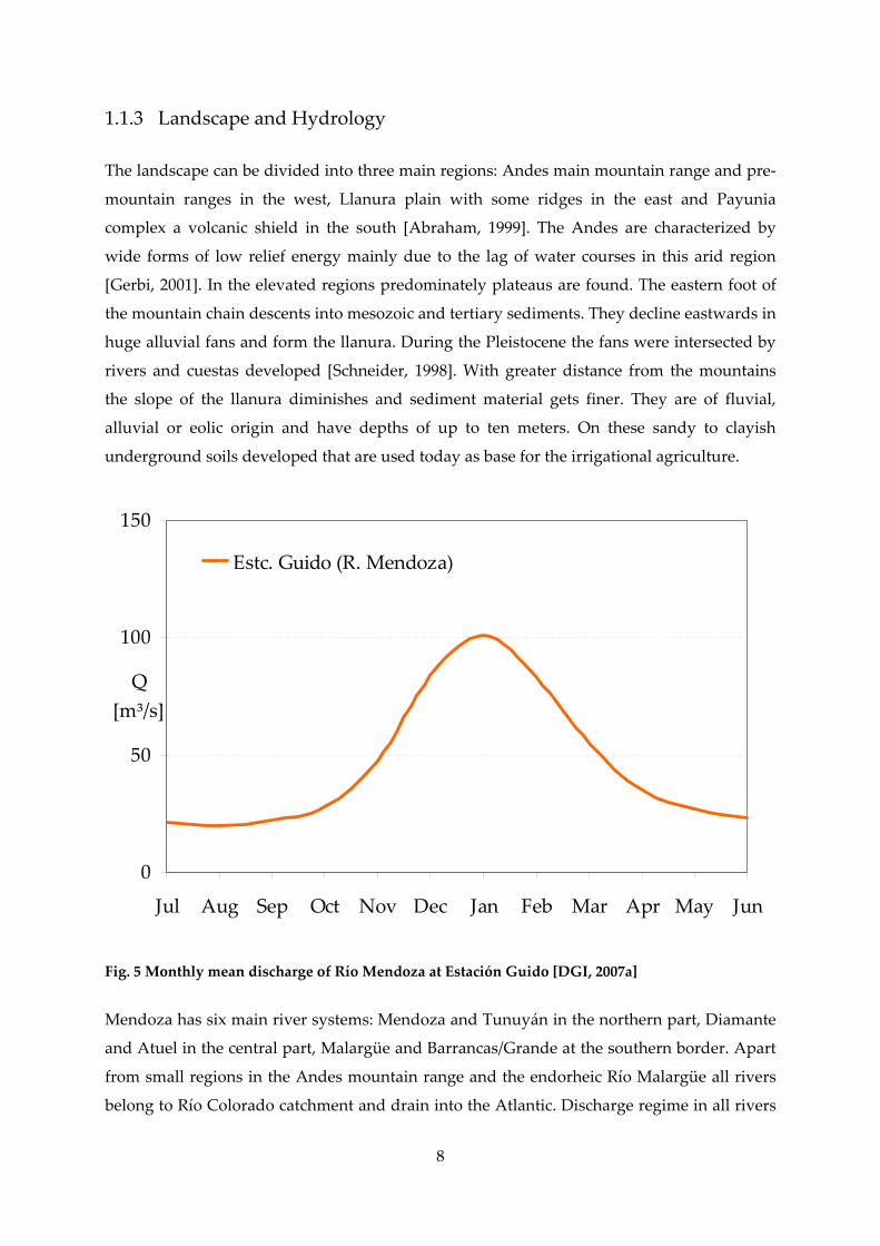
Fig. 5 Monthly mean discharge of Río Mendoza at Estación Guido [DGI, 2007a]
Mendoza has six main river systems: Mendoza and Tunuyán in the northern part, Diamante
and Atuel in the central part, Malargüe and Barrancas/Grande at the southern border. Apart
from small regions in the Andes mountain range and the endorheic Río Malargüe all rivers
belong to Río Colorado catchment and drain into the Atlantic. Discharge regime in all rivers
8
9
is nival [Gudiño de Muñoz, 1991], with mean flow maxima during the summer when snow,
glacier and frost melting water feeds the rivers. [Peter, 1998] points out that water yield in
the oasis mainly depends on storage changes above the snow line and that without the
availability of these resources the existence of the oasis would be unthinkable. Since the
1980’s a constant loss in the mass balance of glaciers described [Leiva, 2007]. [Corripio; 2007]
found that although melting water availability increases in the medium term, accelerated
glacier depletion will cause a strong reduction of annual discharge in the long term.
In addition to the snow and ice melt, summer months December to February have highest
precipitation rates (compare above). The annual hydrograph shows a pronounced peak in
the warmest months. Fig. 5 shows the hydrograph at Estación Guido, the last gauge before
Potrerillos reservoir controls discharge course, the reference period is 1956 – 2006 [DGI,
2007a]. Summer storm events may cause extreme floods that occasionally cause big damages
[Rodríguez Aguilera, 2006] discharges. Up to 15 000 m³/s are reported for Río Mendoza
[Montes, 1995].
Aside from Río Grande flow patterns are heavily influenced by human activity. As a
consequence it is the only river that discharges perennially. Flow in the other rivers is limited
by infiltration, evaporation and extraction [Schneider, 1998]. Almost 2000 hm³
[Chambouleyron, 2000] of storage capacity was created by dams, used for both irrigation
regulation and to generate hydroelectric energy.
The Northern groundwater catchment covers an area of 22800 km². It consists of sediments
mentioned above. The grain size distribution within the area correlates with the surface
slope that decreases from NE to SW [Hernández, 2006a]. The groundwater flow is
consequently rectangular to this direction. The Andes pediment is dominated by coarse
material; it constitutes the main GW recharge zone and the aquifer is unconfined. Surface
slope lowers with increasing distance from the mountain range and with that grain size gets
smaller and the substratum is less permeable. In a transition zone resurgence occurs. Further
southwest clay lenses are found that partly cause semi‐confined aquifer comportment. The
groundwater resources along the rivers Mendoza and Tunuyan have been estimated at
around 490 000 hm³ but only 13 500 hm³/a or 3 % are recharged annually [Zambrano, 1999].
In contrast [Hernández, 2006a] gives 275 000 hm³ of stored recourses and only 7000 hm³ as
recharge rate. [Forster, 2005] estimates that in average 8 500 hm³/a are recharged by the river
courses and another 4 000 hm³/a by reinfiltration of irrigation water. The strongly varying
numbers denote the uncertainty about this resource.

10
1.1.4 Socioeconomic Conditions
Population growth and urbanization determine the population dynamics in Mendoza
province. The number of inhabitants in the city of Mendoza and the surrounding
agglomeration Gran Mendoza, raised between 1981 and 2001 from 613 000 to 849 000
corresponding to 39% increase [INDEC, 2002]. Until 2015 a further growth by 15 % is
expected on the provincial scale [INDEC, 2005]. Within this total increase of population an
additional concentration in urban settlements is registered, accelerating the population
growth in Gran Mendoza. As mentioned above the distribution of population is extremely
heterogeneous, within the oasis population density is with 300 capt./km², the actual
urbanization degree is 80 % [DEIE, 2007].
The most dynamic population growth took place at the beginning of 20th century.
Immigrants from Spain, Italy and the Eastern Mediterranean region, mostly farmers and
cultivators, adapted the existing social and economic structures and favored traditions from
their home countries [Chambouleyron, 1992].
Until today formative agricultural activities that are also characteristic for the province, are
viniculture with 56% of the cultivated land participation, followed by fruit cultivation,
horticulture and olive plantations. 25% of the manufacturing industry is connected to wine
making and the elaboration of fruit and vegetables. Another important activity is the
extraction and refinement of petroleum contributing in 14% to the total national production.
[DEIE, 2007]
Water consumption in Argentina accounts to 300 – 500 l/(d capt) [Mendieta, 2007], in
Mendoza it is estimated to be 400 l/(d capt) [Montaña, 2008] or even 600 l/d [OSM, 1996].Due
to increasing standard of living and economic development this number still tends to rise,
although environmental awareness and sustainability concepts are developing
[Chambouleyron, 2003]. Hence wastewater amounts increase in the private as well as
industrial sector.
1.1.5 Irrigation system and silviculture
Mendoza’s irrigation system creates the largest oasis in Latin America [Peyke, 1989]. Origins
of irrigation along Río Mendoza date back to the pre‐Columbian time. The indigenous
Huarpes used the river for the irrigation of the cultivation of corn [Schneider, 1998]. The

Spanish colonialist basically relied on this existing system and expanded it. Not until the end
of the 19th century the irrigation system was conceptualized and managed using the waters
of Mendoza and Tunuyán rivers jointly and thus creating the Oasis Norte. With the great
immigration wave around 1900 agriculture was adapted to the Mediterranean model
emphasizing wine, olives, drupaceous fruit and vegetables in the cultivation schemes at the
same time the predominance for viticulture rises [Chambouleyron, 1990].
DGI is a state agency that manages the administration of water bodies in Mendoza province.
It controls supervision, evaluation and development of the valorisation of hydrological
resources as well as their use and protection. Water use rights for irrigation, hydroelectricity
and industrial and domestic water supply are given as temporary concessions. The share of
the water amount depends on actually available yield.
Specifications about the surface actually irrigated vary considerably between 2964 km²
[DEIE, 2001a] and 3400 km² [DGI, 2005]. The system consists of 8000km of primary and
secondary canal system [Chambouleyron, 1990]. Of these, only 500 km are concrete‐lined; the
others are earth‐lined. In the lower parts of the irrigation systems, there is also an extensive
network of drainage collectors, with a length of 2 500 km approximately. [Querner, 2008]
found that great part of the groundwater recharge in the plain, that causes locally elevated
phreatic levels is caused by infiltration from the irrigation channels. By comparison of
irrigated area and available water resources, overall efficiency accounts to only 38 %
[Chambouleyron, 1990]. [Marre, 1998] proposes a reformation of cost distribution and claims
the need for higher shares for system maintenance, especially in for the distribution system.
11
( )
combined28%
groundwater21%
surface water51%
y ( )
surface water39%
groundwater28%
combined33%
Fig. 6 Portions of water sources in irrigation for Río Mendoza (left) and Tunuyán Inferior (right)

12
In the Oasis Norte 40000hm³ of groundwater recourses are available. They are mostly
exploited between 100m – 300m depth from more than 25000 wells registered at DGI [DGI,
2005]. About 50 % of Mendozas irrigation area relies at least partly on groundwater
(compare Fig. 6) [Foster, 2005]. In 1990 50m³/s were pumped from groundwater wells
[Thomas, 1998], although the rate strongly depends on annual river discharge [Hernandez,
2006a]. They tap three aquifer levels. The surface aquifer (0 – 80 m below surface level)
provides water of 1 to 2.2 dS/m conductivity, in some zones the value reaches up to 5.5 dS/m,
indicating stronger influence of salinity. For this reason the 2nd (100 – 180 m bsl) and 3rd
(below 200 m bsl) are harvested, where salinity levels are generally lower [Hernandez,
2006a]. Excess water in irrigation evaporates or contributes to groundwater recharge.
Drainage is applied mainly in the Llanura, where soil texture is finer and Halosols are more
common. There are 1800km of drainage collectors installed [Chambouleyron, 1990].
Forestry does not count to the classical industries present in Mendoza. Natural conditions do
not favor the growth of trees and timber is not among the crops historically grown by the
developers of Mendozas irrigation system [Chambouleyron, 1990]. It accounts with 178 km²
[DEIE, 2001a] for about 5 % of the total cultivated area. Nevertheless, due to the intensive
form of cultivation Mendoza contributes to 3 % of total wood production and 43 % of
production of poplars and willows in Argentina [SAGPyA, 2007]. The poplar is by far the
most important cultivated tree; it covers 95 % of all silvicultural area [Calderon, 2006]. In the
period of 1971 to 2001 the forestry plantations almost doubled their extension, indicating a
rising importance of this resource. Especially the production of high quality wood is a recent
focus [Calderón, 2006]. The growth of trees for biomass harvesting is in a state of research
[Bustamante, 2008].
1.2 Problems and Vulnerability related to Water Use
“Historically, both growth and progress of the population of Mendoza have been made
possible by irrigated agriculture. The expansion of irrigated land has reached a critical stage
from both, economical and physical point of view. A wealth of problems has emerged”
[Menenti, 1988].
The proceeding quote emphasizes the importance of irrigation for Mendoza and concludes
the motivation to create this work. Irrigation and the concerted use of water are more than
just a major branch of local business; they are the vital base for all human activity in the

13
zone. But due to contrasting focuses conflicts occur about water use. [Montaña, 2008]
concludes the following:
− natural scarcity of water is exacerbated by steady increase of demand and
diversification; deficits in the coverage of water supply and sewer networks
− low level in water use efficiency, overall efficiency of between 30 and 40 % in the
agriculture, in urban water supply a consume of some 400 l/(d*capt) are reported of
which 75 % return as domestic effluents
− deficit in the coordinated management of superficial and subterranean water
resources
− notable increase of contamination as well of surface water bodies as of aquifers (due
to urban waste disposals, urban and industrial waste waters , hydrocarbons,
salinization)
− split institutional competences in water management and lag of public participation
− insufficient credible information and lag of qualified human resources
− lag of incentives for efficient water use in all consumption
[Hernández, 2006a] concludes the main problems of Mendozas water recources as:
contamination from petrol industry; salinization of the aquifers by agriculture and sediment
deficit problems related to Potrerillos reservoir.
1.2.1 Salinization and hydro‐saline balance
The productivity of one third of all irrigated land is negatively affected to some degree by
salinity [Boyer, 1982]. This number tends to increase as more and more unsuitable land is
applied for irrigation and irrigation projects fail due to salt accumulation in the ground
[Tanji, 1990].
[Aragüés, 1990] points out that sustainable irrigation systems in arid regions are difficult to
maintain as waterborne salt tends to accumulate in the rooting zone. Salt accumulation has
negative effects on soil structure e. g. reduced infiltration, poor aeration and poor water
retention but also on plant physiology e. g. due to toxic effects of sodium ions. The osmotic
component of water potential is linearly proportional to the electric conductivity, e. g. if the
14
EC in the soil solution increases from 1 dS/m to 3 dS/m, osmotic potential decreases from
‐300 cm to ‐1000 cm [Neumann, 1996], or according to [Borg, 2001]1 from ‐430 to ‐1100 cm.
A lot of investigation is done to trigger this subject. Monitoring of salinity in groundwater
[Hernandez, 2006a], phreatic water [Mirábile, 1997], [Ortíz Maldonado, 2005] and soil
[Mirábile, 2003], [Morábito, 2005], [Mastrantonio, 2006] are conducted.
Surface water of 0.3 – 1.8 dS/m deteriorates downstream of Río Mendoza, within a range that
does not affect irrigation purposes [Chambouleyron, 1990]. Before entering the irrigation
distribution system electric conductivity of the Río Mendoza is less than 1 dS/m [Ortíz
Maldonado, 2005] corresponding to roughly 0.3 mg/l NaCl.
Groundwater quality varies considerably, depending on area and depth of exploitation
[Chambouleyron, 1990]. 80% of the groundwater cannot be used, because of poor water
quality [Querner, 1997], basically because of salinity problems.
1.2.2 Excess exploitation of the groundwater
In Mendoza, groundwater is exploited in an area of 5300 km². The level of the water table
generally varies between 10 and 30 m. But in large areas, especially under intensive
agricultural use, depths are more shallow [Querner, 1997].
Assuming the figures mentioned in section 1.1.5, an irrigational water consumption of
1500 mm/a and a total irrigation efficiency of 40 %, an area of 720 km² could be supplied
sustainably with groundwater only2; if the groundwater recharge rate stated by [Hernandez,
2006a] is correct of only 400 km². While [Querner, 1997] mentions that 800 km² are irrigated
with groundwater only and another 300 km² applies both, ground‐ and surface water. The
numbers given by [Hernandez, 2006a] suggest much higher proportions. In areas with
surface water irrigation, there is in principle no need to use supplementary groundwater.
1 [Borg, 2001] proposes the relation that osmotic potential in centimeters is proportional to salt
concentration in grams per liter by factor 760.
2 Equation is: recharge volume divided by irrigation volume per area multiplied with irrigation
efficiency and 20 % usable groundwater.
15
However, because of the misallocation of surface water, the need for groundwater exists,
especially when vegetables are grown [Baars, 1993]
DGI registered in 1994 about 18 200 wells in Mendoza province, of which only 8 900 are in
use. The mean discharge of a well is about 50 l/s [Querner, 1997] and its use depends on the
water need of the crop according to the farmerʹs criteria. About three quarters of these wells
penetrate the Northern Aquifer [DGI, 1994]. Assuming these figures a mean global extraction
rate would be 445 m³/s although it is not clear if this refers only to irrigation season or if it is
an annual mean. In comparison with the value of 50 m³/s mentioned by [Thomas, 1998] again
big uncertainty is revealed. The costs of using groundwater are about 3 to 4 times higher
than for surface water and depend on the costs of electricity and the efficiency of the
pumping equipment.
1.2.3 Oil production and industry
Mendoza accounts for 13 % of the Argentinean oil dwelling and 3 %of natural gas
production. In 2002 Mendoza was the province with the fastest growing production rates,
with 11 % annual growth [Sivera, 2003]. At the same time it’s a mayor center of refinement
and processing of petroleum products and has Argentines biggest refinement complex
[Scheimberg, 2007].
Petroleum hydrocarbons (PHC) consist of alkanes, aromatics (BTEX – benzene, toluol,
ethylbenzene and xylene) and polycyclic hydrocarbons (PAH) [Cummins, 2001]. BTEX and
PAH’s are declared pollutants. BTEX are volatile organic compounds found in petroleum
derivatives, they have harmful effects on the central nervous system and benzene is
carcinogenic and effects the blood circulation. PAH’s consist of fused aromatics, nautrally
they occur in oil, coal and tar deposits. PAH’s are of concern because some compounds have
been identified as carcinogenic, mutagenic, and teratogenic. The petroleum deposits in the
Mendoza area generally produce heavy oils [Ercoli, 2001], they are a main source of PAH’s.
Due to neglectable natural groundwater recharge rate, the threat for the aquifer is not urgent.
Nevertheless this problem may increase if climatic boundary conditions change. Another
path of contamination may occur throughout the spatial vicinity of Río Mendoza to the Oil

16
production fields. 28 cases of petroleum contamination were reported between 1996 and 2003
to the Direction of Sanitation and Environment3.
1.2.4 Unmonitored reuse of waste water
In Mendoza wastewater treatment is conducted with stabilization lagoons. They represent an
uncontrolled physical‐biological treatment method. In the lagoons mainly organic and
hygienic contamination is reduced by solar UV‐radiation and the activity of heterotrophic
organisms. The output discharge is, under regular operation conditions, hygienically safe
and rich in nutrients, making it a valuable water source for irrigation purposes [FAO, 1995].
The use of wastewater for agriculture in Mendoza is limited to especially registered areas,
the ACRE (Area de Cultivos Restringidos Especiales). The uncontrolled nutrient content
causes a main thread for the reuse of pretreated wastewater. It may exceed the actual
demand of plants. Especially during the winter, when irrigation water demand is much
lower while supply is rather constant throughout the year, a mayor fraction of the irrigation
water passes the ground without reduction of nutrient load. Nitrate is of special importance
as it is not retarded a lot in the soil and is under certain circumstances toxic for human health
In Mendoza elevated concentrations of nitrate were monitored in shallow groundwater
layers in the vicinity of the ACRE [Fasciolo, 2006] but no transport to the profound aquifer
could be proved.
[Masotta, 1992] did some work on the evolution of soils under irrigation with pretreated
waste water in the environment of “Campo Espejo” treatment facility. In an comparison of
virgin soil and soils after 5 years of irrigation he found increases of heavy metals (namely
Cadmium, Zinc and Lead) and nutrients (total N and total P) that varied considerably
between different observation points. The increases could by partly explained with the
different soil types occurring. Salinity de‐ or increased on different
The use of viticultural effluents for irrigation purposes is common practice in Mendoza.
These waters have usually high organic charges but may also contain plant treatment
3 Information from http://www.saneamiento.mendoza.gov.ar (site of the sanitation direction, visited
19.12.2008

17
products and other substances. The treatment of these effluents is still uncommon [Bloch,
2000] and an impact study of the effects on soil and water recourses not available.
1.3 Previous Works 1.3.1 State of science in water and mass transport dynamics
[Perry, 2001] describes a similar methodology for water balance modeling to the one applied
in this project. He calibrates a hydrologic model for runoff prediction using soil moisture
data measured on a roughly biweekly basis.
[Maddock, 1998] proposes a measurement setup that permits the integral registration of the
water cycle on basin scale. By coordinated measurement of groundwater, stream flow and
near stream soil moisture and a coupling with LIDAR‐determined evaporation, each in the
process relevant resolution, a closed balance can be set up.
[Kavazanjian, 2006] highlights the problems of unsaturated flow models to represent arid
conditions. Under arid conditions and extremely dry top soils he concludes that difficulties
in accurately measuring small values of percolation on one side and the inability of
unsaturated flow models to accurately predict surface runoff prevent a consistent possibility
to calibrate coupled surface – unsaturated zone models. Although flux values predicted
using models calibrated solely upon internal soil moisture content data are of questionable
reliability, they represent the “lesser of two evils”
1.3.2 Projects related to agricultural water use in Mendoza
Literature was reviewed extensively in order to sort the present work into a regional context
as well as into the state of science. Especially projects carried out in Mendoza and / or by
local institutions were focused. A lot of the relevant works were already mentioned in the
preceding two sections thus this chapter aims to give some structural analysis on research
focus in Mendoza.
Due to the importance of water management tasks for Mendoza oasis, a widespread range of
investigation projects is carried out in the region. Basically themes of agricultural as well as
industrial water management practices and related contamination processes were focused.
Certain tendencies in the thematic orientation of the investigation projects can be appointed,
namely:

18
− large‐scale measurement campaigns rather than localized works
− taking of an inventory rather than process‐orientated measurement
− single task projects rather than integrated cycle‐orientated approaches
Due to the large extensions of Mendoza’s irrigation area, investigation projects often head to
give an overview on a present state or the evolution of certain tendencies e. g. [Mirábile,
2003], [Mastrantonio, 2006]. These projects often compare states of a delimited area
throughout several years. The two mentioned works compare changes in soil salinity
distribution in a period of six or 17 years respectively. But, as working capacities are limited,
there are hardly any projects that reach an adequate temporal resolution which allows
estimating the dynamics of hydrological processes.
[Morábito, 2004] states the lag of coordinated and systematized measurements of
information related to integral determination of water resources and irrigation efficiency.
This problem can’t be triggered only on a technical level. [Foster, 2005] proposes institutional
and administrative measures for integrated groundwater resource conservation in the
Mendoza aquifers.
Modeling is still not a common practice in the scientific community engaged in water
resource management. Although this field of work is strongly emerging. Some projects have
been conducted to represent aquifer [Hernández, 2006b], channel system [Menenti, 1995],
irrigated fields [Salomon, 2007], [Mirábile, 2006]. [Querner, 1997] emphasizes the importance
of a stronger focus on coupling of different subsystems and integrated projection for the
irrigation system of Mendoza and suggests an approach for lower Tunuyán River. [Menenti,
1995] showed in a conclusion the application of different surface runoff models at Mendoza.
A conceptual approach to the integral representation of surface flow, unsaturated zone and
groundwater is given by [Querner, 2008].
1.3.3 Poplars and their interaction with the environment
Poplars are capable to adapt to a broad range of climatic conditions and changing
environments [Gilen, 2001]. They are therefore grown for wood and biomass production in
Mendoza region, often on sites where other crops appear unsuitable. [Shannon, 1998]
mentions the capability of some poplar clones to cope with conditions of elevated salinity, he
states that some hybrid poplars are able to cope with salinities as high as 14 g/l NaCl,
corresponding to a conductivity of more than 50 dS/m. This additionally raises the value of

19
this crop for Mendoza area, e.g. on halosol‐sites or for drainage‐ and wastewater recycling.
In contrast [Neumann, 1996] describes poplars as more sensitive to elevated salinity than
other irrigated tree species but also variability of salt resistance is high, values between 1 –
5 dS/m are mentioned, to compare for eucalyptus resistance range is 10 – 25 dS/m.
Water demand of poplars is elevated. Some figures are given in section 2.2.7 below.
Compared with the listing given in [Chambouleyron, 1991] they belong to the crops with the
highest water demand in Mendoza. [Neumann, 1996] names poplars as silvicultural crop
with the highest potential water demand. In the context of Phytoremediation poplars are
called “solar pumps” for their high capacity of water suction from the phreatic water table
The combination of elevated irrigation volumes and high salinity potential of as well of the
irrigation water as of the plant site indicate the risk of poplar plantations for groundwater
salinization. Due to badly managed irrigation schemes or leaching at these plantations, salt is
washed into the soil zone below capillary rise. Possible consequences are an elevation of the
water table and following salinization of the surface or constant salt washout into the
aquifer.
Roots functionally transmit water from the soil to the metabolically active parts of the plant.
[Thomas, 2008] shows the importance of transpiration rate for the water balance of soils. He
compares soil water dynamics between a hedgerow and surrounding bare areas and reveals
that water dynamics differ importantly as well temporally as spatially. Under the hedges he
generally finds more amplitude in total water consumption and a less pronounced reduction
of amplitude with depth.
[Mulia, 2005] found that poplar roots are highly sensitive for heterogeneous environmental
conditions. In his research, conducted in southern France, he found that regularly root
distribution decreased with depth and distance from the stem but in situations of growth
concurrence by intercrops or unfavorable soil conditions in the upper layer, root distribution
was reverted. [Tschaplinski, 1998] shows that higher seasonal irrigation volumes have a
slight effect on denser root distribution and considerable effect on lower root to stem weight
ratios. These two factors indicate that, while root growth is weakly effected by different
irrigation regimes, stems show more growth when watered more intensely. Conductance
tests indicate that water uptake of poplar roots is strongly reduced under flooded soil
conditions [Pregitzer, 1996]. Distribution and performance of poplars roots were so far not in
the focus of research in the Mendoza region. Hence only scarce information is available
20
about root distribution and water uptake at root level. [Riu, 1993] captured this relation
conceptually by level‐wise determining water storage change in the soil.
[Li, 2006] states that straightforward coupling of water uptake to root distribution, as
realized by the SiWaPro implemented [Feddes, 1978] model, does not reproduce adequately,
processes especially in dry periods. Upper soil layers are densely rooted and they dry fastest,
hence in these drought periods water uptake is realized more intense by lower roots.
[Hopmans, 1998] presents a tool for the coupled modeling of soil water and root dynamics.
He concludes that integrated parameter estimation for the water movement in soil and
uptake by roots as well as root growth corresponds basically to a gray box approach of
model calibration. At the actual state of knowledge spatial resolution of data acquisition and
measurement of fine root water flow are the bottleneck for enhanced system understanding.
It is worth mentioning that root dynamics and root water uptake modeling is carried out at
the moment on three different spatial scales: plant e.g. [Tschaplinski, 1998], [Durso, 2004] site
[Abrahamson, 2005], [Verstraeten, 2005] and regional to global scale [Kalma, 1999]. [Feddes,
2001] points out the problems in scale transition and [Li, 2006] confirms that modeling results
o different spatial levels are often not consistent. It is thus valuable to compare modeling
results on different scales in order to enhance system comprehension.
1.4 Model Description
The mathematical model behind SiWaPro [Kemmesies 1999] is based on the computational
core used in SWMS 2D [Šimunek 1994]. The model core was developed to simulate water
and solute movement in variably saturated media. The software consists of the SiWaPro
computer program, a graphical ‐ and a database interface, soil, climate and contaminant
databases, a weather generator and subroutines for the estimation of hydraulic and mass
transport parameters. The SiWaPro program numerically solves the Richards equation for
variably‐saturated water flow and the convection‐dispersion type equations for solute
transport. The flow equation incorporates a sink term to account for water uptake by plant
roots. Hysteresis can be represented by a scaling parameter. Adsorption and decomposition
may be considered as substance transformation processes.
Main parts of this section refer to SiWaPro [Blankenburg, 2008] and SWMS 2D [Šimunek
1994] and HYDRUS‐2D [Šimunek 1999] handbooks in their most recent available version.

1.4.1 Physical base of flow and mass transport
SiWaPro computes water and mass transport physically based. Elementary laws of dynamics
and mass conservation are combined in Richards Equation in order to flow in porous media.
Convection‐Dispersion‐Equation (CDE) computes mass transport process but is equally apt
to describe heat transport in the ground.
Description of flow in porous media
Flow conditions of fluids in partly saturated media can be described by combining the
fundamental law of dynamics with the corresponding balance equation. Governing forces
for the flow in porous media are gravity, pressure and friction. Darcy’s Law (F. 2) concludes
the balance of forces as given in F. 1. Friction, viscosity and density are concluded in a
material specific constant‐ the coefficient of permeability of saturated conductivity k.
⎟⎟⎠
⎞⎜⎜⎝
⎛∂∂
+∂∂
ρ=
ηρ
=
=η+∂∂
ρ+∂∂
xz
xp
g1kv:follows
Cg
k:with
0vCzxg
xp
xx
xx
xx
F. 1
F. 2
with: p pressure [M/L²]
x coordinate of direction [L]
ρ density of the fluid [M/L³]
g acceleration of gravity [L/T²]
z coordinate of direction of gravity [L]
Cx coefficient of friction [1/M²]
η dynamic viscosity [M²/LT]
vx velocity of flow in direction of x [L/T]
kx coefficient of permeability in direction of x [L/T]
Mass balance continuity for the observation volume is an expression of the law of mass
conservation. It states that water content of the volume is completely defined by in‐ and
outflow to the volume, storage change within the volume and sinks and sources.
21
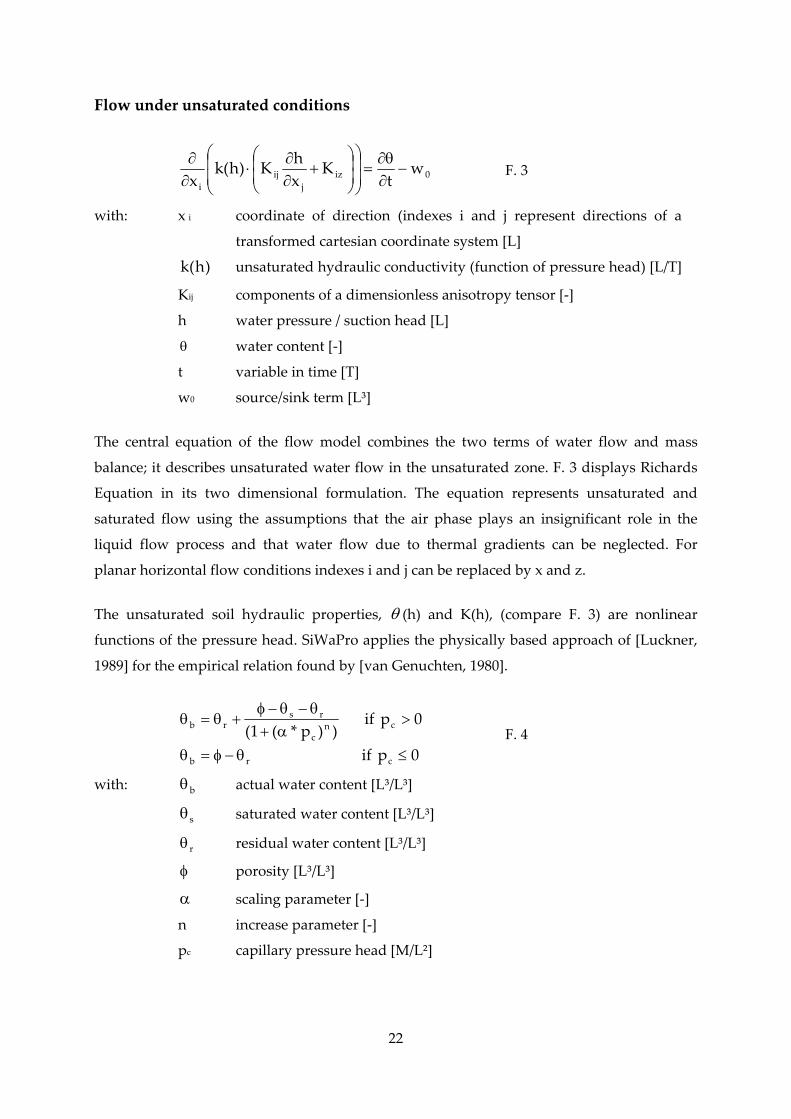
Flow under unsaturated conditions
0izj
iji
wt
KxhK)h(k
x−
∂θ∂
=⎟⎟
⎠
⎞
⎜⎜
⎝
⎛⎟⎟⎠
⎞⎜⎜⎝
⎛+
∂∂
⋅∂∂
F. 3
with: x i coordinate of direction (indexes i and j represent directions of a
transformed cartesian coordinate system [L]
unsaturated hydraulic conductivity (function of pressure head) [L/T]
Kij components of a dimensionless anisotropy tensor [‐]
h water pressure / suction head [L]
water content [‐]
t variable in time [T]
w0 source/sink term [L³]
)h(k
θ
The central equation of the flow model combines the two terms of water flow and mass
balance; it describes unsaturated water flow in the unsaturated zone. F. 3 displays Richards
Equation in its two dimensional formulation. The equation represents unsaturated and
saturated flow using the assumptions that the air phase plays an insignificant role in the
liquid flow process and that water flow due to thermal gradients can be neglected. For
planar horizontal flow conditions indexes i and j can be replaced by x and z.
The unsaturated soil hydraulic properties, θ (h) and K(h), (compare F. 3) are nonlinear
functions of the pressure head. SiWaPro applies the physically based approach of [Luckner,
1989] for the empirical relation found by [van Genuchten, 1980].
0pif
0pif))p*(1(
crb
cnc
rsrb
≤θ−φ=θ
>α+
θ−θ−φ+θ=θ
F. 4
with: actual water content [L³/L³]
saturated water content [L³/L³]
residual water content [L³/L³]
porosity [L³/L³]
scaling parameter [‐]
n increase parameter [‐]
pc capillary pressure head [M/L²]
bθ
sθ
rθ
φ
α
22
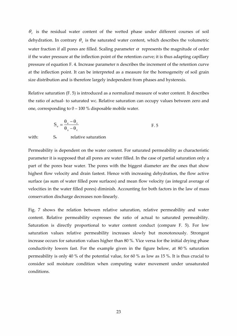
rθ is the residual water content of the wetted phase under different courses of soil
dehydration. In contrary sθ is the saturated water content, which describes the volumetric
water fraction if all pores are filled. Scaling parameter α represents the magnitude of order
if the water pressure at the inflection point of the retention curve; it is thus adapting capillary
pressure of equation F. 4. Increase parameter n describes the increment of the retention curve
at the inflection point. It can be interpreted as a measure for the homogeneity of soil grain
size distribution and is therefore largely independent from phases and hysteresis.
Relative saturation (F. 5) is introduced as a normalized measure of water content. It describes
the ratio of actual‐ to saturated wc. Relative saturation can occupy values between zero and
one, corresponding to 0 – 100 % disposable mobile water.
rs
reeS θ−θ
θ−θ= F. 5
with: Se relative saturation
Permeability is dependent on the water content. For saturated permeability as characteristic
parameter it is supposed that all pores are water filled. In the case of partial saturation only a
part of the pores bear water. The pores with the biggest diameter are the ones that show
highest flow velocity and drain fastest. Hence with increasing dehydration, the flow active
surface (as sum of water filled pore surfaces) and mean flow velocity (as integral average of
velocities in the water filled pores) diminish. Accounting for both factors in the law of mass
conservation discharge decreases non‐linearly.
Fig. 7 shows the relation between relative saturation, relative permeability and water
content. Relative permeability expresses the ratio of actual to saturated permeability.
Saturation is directly proportional to water content conduct (compare F. 5). For low
saturation values relative permeability increases slowly but monotonously. Strongest
increase occurs for saturation values higher than 80 %. Vice versa for the initial drying phase
conductivity lowers fast. For the example given in the figure below, at 80 % saturation
permeability is only 40 % of the potential value, for 60 % as low as 15 %. It is thus crucial to
consider soil moisture condition when computing water movement under unsaturated
conditions.
23
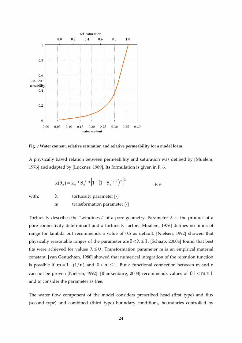
Fig. 7 Water content, relative saturation and relative permeability for a model loam
A physically based relation between permeability and saturation was defined by [Mualem,
1976] and adapted by [Luckner, 1989]. Its formulation is given in F. 6.
( )[ ]2mm/1ee0e S11*S*k)(k −−=θ λ
F. 6
with: tortuosity parameter [‐]
m transformation parameter [‐]
λ
Tortuosity describes the “windiness” of a pore geometry. Parameter λ is the product of a
pore connectivity determinant and a tortuosity factor. [Mualem, 1976] defines no limits of
range for lambda but recommends a value of 0.5 as default. [Nielsen, 1992] showed that
physically reasonable ranges of the parameter are 10 ≤λ< . [Schaap, 2000a] found that best
fits were achieved for values . Transformation parameter m is an empirical material
constant. [van Genuchten, 1980] showed that numerical integration of the retention function
is possible if and
0≤λ
)n/1(1m −= 1m0 ≤< . But a functional connection between m and n
can not be proven [Nielsen, 1992]. [Blankenburg, 2008] recommends values of 1m1.0 ≤<
and to consider the parameter as free.
The water flow component of the model considers prescribed head (first type) and flux
(second type) and combined (third type) boundary conditions, boundaries controlled by
24
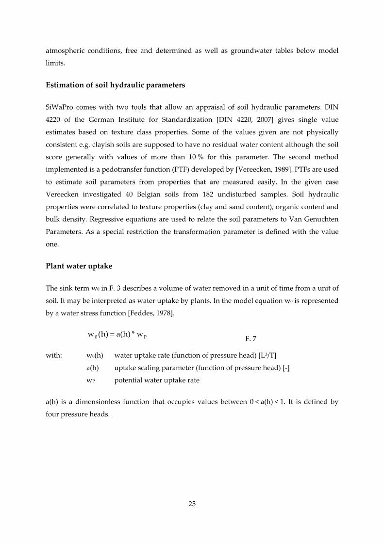
atmospheric conditions, free and determined as well as groundwater tables below model
limits.
Estimation of soil hydraulic parameters
SiWaPro comes with two tools that allow an appraisal of soil hydraulic parameters. DIN
4220 of the German Institute for Standardization [DIN 4220, 2007] gives single value
estimates based on texture class properties. Some of the values given are not physically
consistent e.g. clayish soils are supposed to have no residual water content although the soil
score generally with values of more than 10 % for this parameter. The second method
implemented is a pedotransfer function (PTF) developed by [Vereecken, 1989]. PTFs are used
to estimate soil parameters from properties that are measured easily. In the given case
Vereecken investigated 40 Belgian soils from 182 undisturbed samples. Soil hydraulic
properties were correlated to texture properties (clay and sand content), organic content and
bulk density. Regressive equations are used to relate the soil parameters to Van Genuchten
Parameters. As a special restriction the transformation parameter is defined with the value
one.
Plant water uptake
The sink term w0 in F. 3 describes a volume of water removed in a unit of time from a unit of
soil. It may be interpreted as water uptake by plants. In the model equation w0 is represented
by a water stress function [Feddes, 1978].
P0 w*)h(a)h(w = F. 7
with: w0(h) water uptake rate (function of pressure head) [L³/T]
a(h) uptake scaling parameter (function of pressure head) [‐]
wP potential water uptake rate
a(h) is a dimensionless function that occupies values between 0 < a(h) < 1. It is defined by
four pressure heads.
25
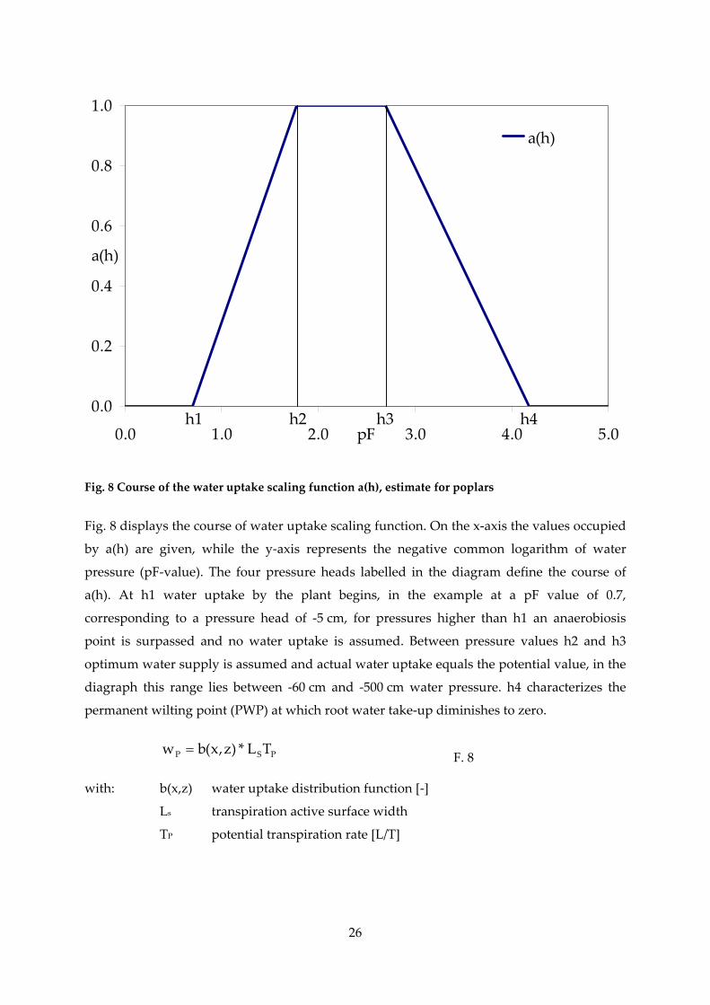
0.0
0.2
0.4
0.6
0.8
1.0
0.0 1.0 2.0 3.0 4.0 5.0pF
a(h)
a(h)
h3 h4h2h1
Fig. 8 Course of the water uptake scaling function a(h), estimate for poplars
Fig. 8 displays the course of water uptake scaling function. On the x‐axis the values occupied
by a(h) are given, while the y‐axis represents the negative common logarithm of water
pressure (pF‐value). The four pressure heads labelled in the diagram define the course of
a(h). At h1 water uptake by the plant begins, in the example at a pF value of 0.7,
corresponding to a pressure head of ‐5 cm, for pressures higher than h1 an anaerobiosis
point is surpassed and no water uptake is assumed. Between pressure values h2 and h3
optimum water supply is assumed and actual water uptake equals the potential value, in the
diagraph this range lies between ‐60 cm and ‐500 cm water pressure. h4 characterizes the
permanent wilting point (PWP) at which root water take‐up diminishes to zero.
PSP TL*)z,x(bw = F. 8
with: b(x,z) water uptake distribution function [‐]
Ls transpiration active surface width
TP potential transpiration rate [L/T]
26

Equation F. 8 represents the distribution of roots in the soil zone. The water uptake
distribution function can be interpreted as a weighting factor that defines the spatial
variation of wP over the root zone. The transpiration active surface expresses what extension
of the soil surface contributes to the transpiration process. Accordingly the potential
transpiration rate expresses the metabolic water output of plant as a flux normalized over the
cultivated surface.
Mass transport description
The program uses Convection‐Dispersion‐Equation to compute mass transport processes.
F. 9 gives the equation for the two dimensional case under the same conventions of direction
as in F. 3. The joint consideration of mobile and immobile phase is only feasible for the
assumption that concentrations in both phases are related linearly.
0wswmmi
i
iij
i
m wcsxcq
)xcD(
xts
−ργ+θγ+μ+∂∂
−∂∂
θ∂∂
=∂
∂
F. 9
with: sm substance mass (combining mobile and immobile phase)
Dij dispersion coefficient tensor [L²/T]
c concentration in the mobile phase [M/L³]
qi water flux towards i (normalized by volume) [M/L]
first order decomposition constant (mobile and immobile) [1/T]
mμ
wγ zeroth order decomposition constant for mobile phase [M/L³T]
sγ zeroth order decomposition constant for immobile phase [1/T]
solid phase bulk density [M/L³]
cw source / sink concentration [M/L³]
ρ
Equation F. 9 can be solved if water content and flux through the volume are known. Both
values are computed by Richardson Equation as given in F. 3.
Mass transport parameters are user specified. A data base of currently more than 100
substances is incorporated. Transport parameters of dispersion, decomposition and
adsorption are estimated based on organic content, soil pH and clay content.
27

28
1.4.2 Numerical solution of the governing equations
Flow and transport equations are solved numerically using Galerkin‐type linear finite
element schemes. The observation area (2D case) is discretized into an irregular triangular
network. The corner points of the adjacent triangles serve as nodal points for the
computations.
Discretization
For each nodal point the dependent variables of the governing equations F. 3 and F. 9 are
approximated by a finite series of linear basis functions. They are required to meet the
condition of a minimum deviation between linearized and exact solution. The linear
approaches are introduced into the governing equations and integrated over all elements
and boundaries of the observation area. This leads to a system of ordinary differential
equations. The solution for the triangular elements is realized by a weighting of permeability
and storage volume over the corner nodes.
Temporal derivates are represented by finite time differences. For water dynamics modeling
an implicit scheme is used for the solution under saturated and unsaturated conditions. That
means that the solution of the previous time step is used to solve the equation of the actual
one. Initial conditions feed the first time step. For mass transport computation the scheme
can be defined by a time weighting factor that allows solutions to by completely explicit,
implicit or of any weighted scheme in between (e.g. Crank‐Nicholson that accounts explicit
and implicit solution with same weights).
Solution strategies
The non‐linear equations that evolve from the combination of spatial and temporal
discretization matrices are solved by iteration. The boundary conditions for every time step
allow determining the variables matrix values by Gaussian Elimination, where values from
the previous iteration loop are used to calculate variables of the actual one. If the difference
of the calculated pressure heads of two subsequent time steps falls below a predefined
threshold, the result is accepted. The initial estimate of the actual time step is estimated by an
extrapolation from the two previous steps. Besides from iteration threshold mass balance is
controlled for every time step. Time step control is managed dynamically where numerical
stability, dates of changing boundary conditions and output dates are considered. Numerical
29
stability is ensured by adapting time step length to the iteration process of the previous time
step. If the number of iterations surpasses a predefined value, time step length is lowered by
a predefined factor smaller than one. If the number of iterations is smaller than a predefined
number, time step length is raised by a predefined factor. If the number of iterative loops
surpasses a predefined maximum number, computation is interrupted and continued in the
following time step, an error is reported to the operator. For mass transport computation the
solved matrix of water transport is inserted into the mass transport term (compare F. 9 and
corresponding explanation) resulting in a set of linear equations. Depending on the solution
scheme (see above) the equation has to be solved for the actual, previous or both time steps.
Upstream weighting is included in order to minimize numerical oscillation, for further
explanation compare [Yeh, 1990]. Peclet numer and courant number are included for the
control of numeric stability. Courant numbers are communicated program‐internally for the
control of time step lengths.
1.4.3 Input data
SiWaPro requires basically a geometrically defined section of the underground that allows
delimiting influences from the surrounding. Soil information is used to describe the water
and mass transport properties. Hydrological boundary conditions drive the model
computation, with climatic influence being usually the upper condition and groundwater
table determining the lower limit. Mass transport properties are regarded and the temporal
variation of mass sources is taken into account. Optionally source and sink terms, e. g. plant
consumption may be defined.
As climatic data time series of precipitation, evaporation and eventually transpiration are
used. If this data is not available, time series may be generated with a weather generator. For
agricultural drainage cases time series of drainage rates may be defined. Groundwater table
may be considered statically or as a series of time.
For the water uptake by plants root distribution and distributed water consumption are
included.
Resolution of input data may be chosen freely, typical values range from meters to
kilometers in space and minutes to years in time. The operator should keep in mind that the
resolution of input data delimits model purposes. Temporal and spatial resolution should
correspond to the velocity of the processes represented.
30
1.4.4 Limits and possibilities
Spatial and temporal resolution may be defined freely. Time steps are managed adaptively
by the program within defined limits. The finite element discretization allows distributing
model resolution heterogeneously, sections of high dynamics or special interest may be
considered more exactly.
SiWaPro model allows representing heterogeneous soil conditions. Soil properties may be
defined section‐wise or layer‐wise. In the same way anisotropy is considered Due to the
finite element structure different soil properties may be taken into account in the spatial
resolution as well, e.g. soils of higher transport dynamics can be represented with higher
discretization.
The program includes a routine for inverse parameter optimization. Starting from an initial
estimation of soil hydraulic parameters and observed values of water or mass flux at model
boundaries; pressure head or water content at defined points of the model or specific mass
content at a defined point of time.
A weather generator is included into the program. Based on a internal database of German
CSs it is possible to generate series of climate data for any point situated within the
extensions of the database stations. The series are based on the interpolated statistical values
of the CSs.
Often there is a lag of mass transport parameters measured for the investigation site. These
parameters are laborious to determine or samples for the experimental determination are not
available. To solve this gap SiWaPro comes with a data base of mass transport properties.
More than 90 organic and 10 inorganic substances are integrated and PTFs allow considering
site specific soil conditions.
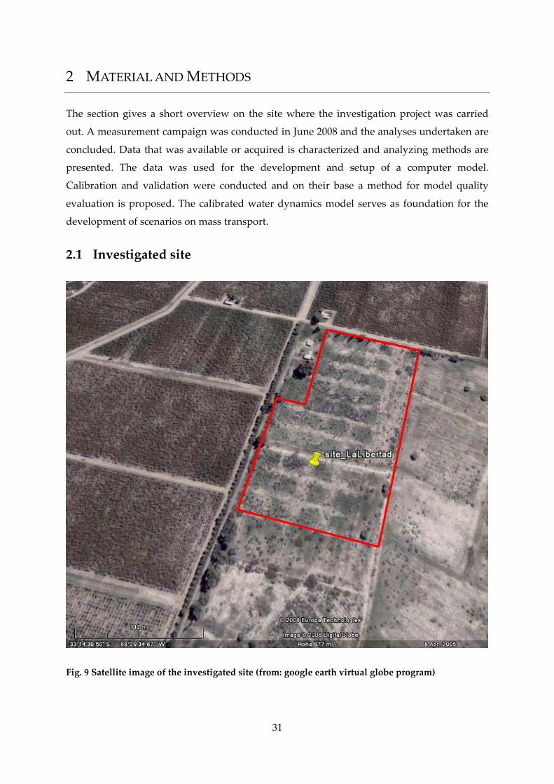
2 MATERIAL AND METHODS
The section gives a short overview on the site where the investigation project was carried
out. A measurement campaign was conducted in June 2008 and the analyses undertaken are
concluded. Data that was available or acquired is characterized and analyzing methods are
presented. The data was used for the development and setup of a computer model.
Calibration and validation were conducted and on their base a method for model quality
evaluation is proposed. The calibrated water dynamics model serves as foundation for the
development of scenarios on mass transport.
2.1 Investigated site
Fig. 9 Satellite image of the investigated site (from: google earth virtual globe program)
31
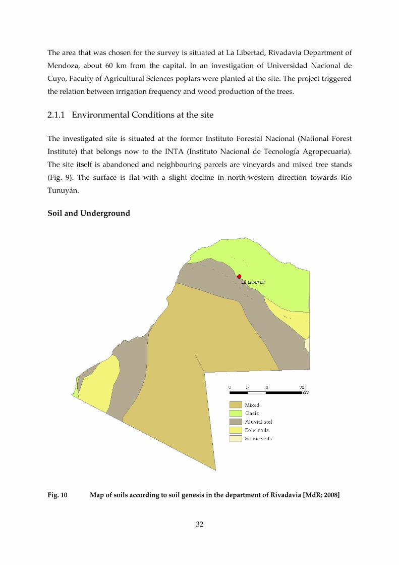
The area that was chosen for the survey is situated at La Libertad, Rivadavia Department of
Mendoza, about 60 km from the capital. In an investigation of Universidad Nacional de
Cuyo, Faculty of Agricultural Sciences poplars were planted at the site. The project triggered
the relation between irrigation frequency and wood production of the trees.
2.1.1 Environmental Conditions at the site
The investigated site is situated at the former Instituto Forestal Nacional (National Forest
Institute) that belongs now to the INTA (Instituto Nacional de Tecnología Agropecuaria).
The site itself is abandoned and neighbouring parcels are vineyards and mixed tree stands
(Fig. 9). The surface is flat with a slight decline in north‐western direction towards Río
Tunuyán.
Soil and Underground
Fig. 10 Map of soils according to soil genesis in the department of Rivadavia [MdR; 2008]
32
The department of Rivadavia is situated partly on a quaternary alluvial fan and partly in the
downstream alluvial plain. Both cover a postglacial fluvio‐lacustrine plain that is exposed in
some parts [Abraham, 1999].
Great pedologic groups occurring are Torripsaments, Torrifluvents and Torriortents, all
three belong to the entisol group Entisols are defined as soils that do not show any profile
development more than an A horizon. An Entisol has no diagnostic horizons, and most are
basically unaltered from their parent material. Although no horizons are determinable,
sedimented soils may well show stratification, due to different deposition periods. [Torre,
2006] mentions those groups as typical for the arid Chaco region.
The soils that are irrigated in the area are mainly alluvial. They are heterogeneous and show
different texture layers. Eolic soils are also fertile but lag organic matter and nitrogen
[Chambouleyron, 1990] and often have a very fine texture. The ground at the site is within an
alluvial zone at the boundary of an extended irrigation region (Fig. 10). Soils typically have
relatively high pH values between 7.2 and 8.5 and organic matter contents of less than 1 %
[Chambouleyron, 2002].
The soil at the site was characterized as sandy loam; measured sedimentation volumes
indicated small heterogeneity. Permanent wilting point and field capacity indicate sandy
loam as well although available water content is with about 11 % more in the range of sand.
Bulk density is medium and soil salinity low.
Tab. 1 Soil properties at La Libertad
SV [ml/g] fc [%] pwp [%] DB [g/cm³] ECe [dS/m]0.85 16 ‐ 19.5 6 ‐ 8 1.5 1.56
La Libertad lies in a zone where the groundwater level is 2.5 m or more meters below surface
(state of 2002) [DGI, 2003]. Local workers from former Estación Forestal Nacional stated that
groundwater was not reachable for the tree roots and irrigation is vivid for the parkscape
with a mature mixed tree population.
33

Climate and Vegetation
Climate basically matches the conditions described for the Llanura in section 1.1.2. The site
has naturally arid climate although oasis effect is likely to occur over irrigated surfaces. [Riu,
2003] gives the values concluded in Tab. 2. It is mentioned that rainfall is concentrated in the
period November to March.
Tab. 2 Climate characteristics at La Libertad
Tm [°C] Tmin [°C] Tmax [°C] rh [%] u [m/s] P [mm/a]15.8 32.1 1.2 60 1.67 204
Fig. 11 Natural vegetation in the surrounding of the investigated site
The natural vegetation in Rivadavia department consists of xerophytic plant communities
and belongs to the Monte ecoregion. [Roig, 1999] mentions the presence of psilophytic and
34
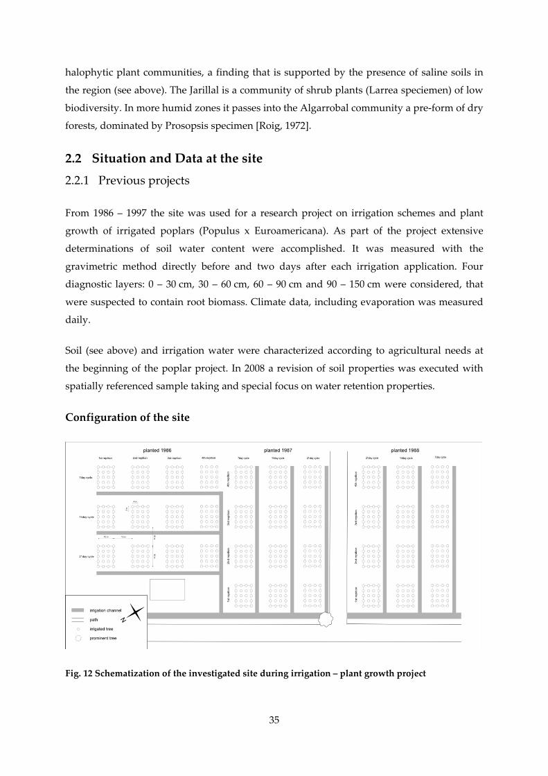
halophytic plant communities, a finding that is supported by the presence of saline soils in
the region (see above). The Jarillal is a community of shrub plants (Larrea speciemen) of low
biodiversity. In more humid zones it passes into the Algarrobal community a pre‐form of dry
forests, dominated by Prosopsis specimen [Roig, 1972].
2.2 Situation and Data at the site 2.2.1 Previous projects
From 1986 – 1997 the site was used for a research project on irrigation schemes and plant
growth of irrigated poplars (Populus x Euroamericana). As part of the project extensive
determinations of soil water content were accomplished. It was measured with the
gravimetric method directly before and two days after each irrigation application. Four
diagnostic layers: 0 – 30 cm, 30 – 60 cm, 60 – 90 cm and 90 – 150 cm were considered, that
were suspected to contain root biomass. Climate data, including evaporation was measured
daily.
Soil (see above) and irrigation water were characterized according to agricultural needs at
the beginning of the poplar project. In 2008 a revision of soil properties was executed with
spatially referenced sample taking and special focus on water retention properties.
Configuration of the site
Fig. 12 Schematization of the investigated site during irrigation – plant growth project
35
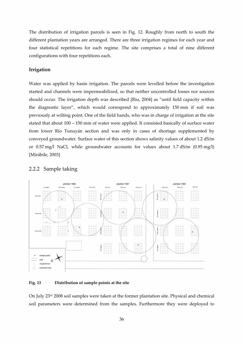
The distribution of irrigation parcels is seen in Fig. 12. Roughly from north to south the
different plantation years are arranged. There are three irrigation regimes for each year and
four statistical repetitions for each regime. The site comprises a total of nine different
configurations with four repetitions each.
Irrigation
Water was applied by basin irrigation. The parcels were levelled before the investigation
started and channels were impermeabilized, so that neither uncontrolled losses nor sources
should occur. The irrigation depth was described [Riu, 2004] as “until field capacity within
the diagnostic layer”, which would correspond to approximately 150 mm if soil was
previously at wilting point. One of the field hands, who was in charge of irrigation at the site
stated that about 100 – 150 mm of water were applied. It consisted basically of surface water
from lower Río Tunuyán section and was only in cases of shortage supplemented by
conveyed groundwater. Surface water of this section shows salinity values of about 1.2 dS/m
or 0.57 mg/l NaCl, while groundwater accounts for values about 1.7 dS/m (0.95 mg/l)
[Mirábile, 2003]
2.2.2 Sample taking
Fig. 13 Distribution of sample points at the site
On July 23rd 2008 soil samples were taken at the former plantation site. Physical and chemical
soil parameters were determined from the samples. Furthermore they were deployed to
36

determine water‐ and mass transport characteristics in the soil zone. During the campaign,
sample points and site geometry were geo‐referenced, using a GPS handheld.
The distribution of the sample points was optimized graphically with the objectives of
reaching a homogeneous distance between the points and a maximum coverage of site by
adjacent circles (Fig. 13).
The derived points were displaced within a radius of 15 m, in order to reach a maximum
variation of the plant configuration. By that the six sample points could be reallocated that
represent each plantation year and irrigation cycle with two points (Fig. 14).
At each point samples were taken at 15 cm, 45 cm, 75 cm and 120 cm below soil surface,
corresponding to the observation horizons mentioned above. In the following, denotation
refers to sample point with the first count and depth with the second count, e.g. soil 5.2 is the
sample taken from the 21d irrigation cycle parcel of the 1986 planted part at 45 cm below
surface.
plantation year →irrigation cycle↓
7d MP 6 MP 2
14d MP 4 MP 1
21d MP 5 MP 3
1986 1987 1988
Fig. 14 Configuration of sample points (MP = measurement point)
2.2.3 Available Data
As mentioned above, the project can be seen in continuation of the works done by the
Faculty of Agrarian Sciences, Universidad Nacional de Cuyo [Riu, 1993], [Riu, 2004] and
others. Hence great parts of the data obtained in these studies could be used.
Soil moisture data was measured directly before and two days after each irrigation donation.
Relative humidity was measured from soil samples with a gravimetric method as proposed
by [ISO 11461, 2001]. Values are available from four depths. Potential evaporation was
detected from a Class A evaporation pan and precipitation with a gauge. Both values were
37

registered with daily resolution. Plants actual transpiration was calculated from evaporation
data and soil humidity dynamics with a resolution with Grassi method (F. 15, below) of each
irrigation cycle and normalized in 15‐day periods.
Estimates for irrigation volumes were available concluding the fact that it was irrigated until
field capacity in the diagnostic layer [Riu, 2003]. The local workers that were responsible for
the application of irrigation water estimated that irrigation depths reached 100‐150 mm.
Irrigation water was analyzed before the plant growth project began.
Evaporation, Transpiration and Precipitation are direct climatic boundary conditions of
SiWaPro program. Resolution requirements should match process dynamics. They
determine possible modeling purposes. For the present work a consistent set of climate and
plant data was elaborated, applying competition and regionalization strategies. The climate
data for the climate stations (CSs) was delivered by Servicio Meteorológico Nacional (SMN,
Argentine National Meteorological Service) and cover the period 01.01.1990 until 31.10.2007.
2.2.4 Preprocessing
The data from the investigation site was on hand in written form. It was digitized partly
using optical character recognition and partly by manual transcription. During this process
data was verified using the plausibility ranges given in Tab. 3
Tab. 3 Plausibility ranges of measured parameters
Parameter Minimum range Maximum rangeEvaporation [mm/d] 0 30Wind Speed [m/s] 0 ‐Sunshine duration [h] 0 18Mean Temperature [°C] ‐30 60Precipitation [mm/d] 0 ‐Relative air humidity [%] 0 100Relative soil humidity [%] 0 50
Climate data that ranged out of these values was completed with data from neighboring CSs
(see below). Soil moisture dates were not considered if values exceeded the limits.
38
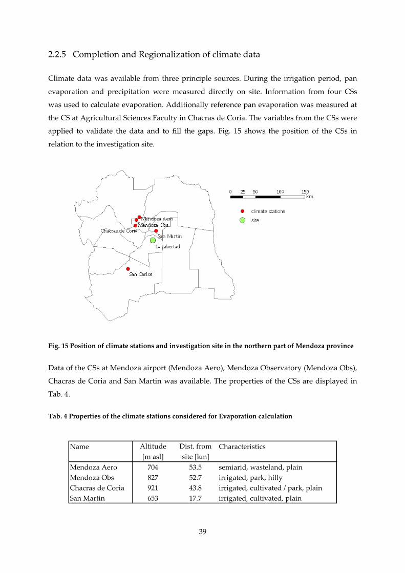
2.2.5 Completion and Regionalization of climate data
Climate data was available from three principle sources. During the irrigation period, pan
evaporation and precipitation were measured directly on site. Information from four CSs
was used to calculate evaporation. Additionally reference pan evaporation was measured at
the CS at Agricultural Sciences Faculty in Chacras de Coria. The variables from the CSs were
applied to validate the data and to fill the gaps. Fig. 15 shows the position of the CSs in
relation to the investigation site.
Fig. 15 Position of climate stations and investigation site in the northern part of Mendoza province
Data of the CSs at Mendoza airport (Mendoza Aero), Mendoza Observatory (Mendoza Obs),
Chacras de Coria and San Martin was available. The properties of the CSs are displayed in
Tab. 4.
Tab. 4 Properties of the climate stations considered for Evaporation calculation
39
Altitude Dist. from[m asl] site [km]
Mendoza Aero 704 53.5 semiarid, wasteland, plainMendoza Obs 827 52.7 irrigated, park, hillyChacras de Coria 921 43.8 irrigated, cultivated / park, plainSan Martin 653 17.7 irrigated, cultivated, plain
Name Characteristics
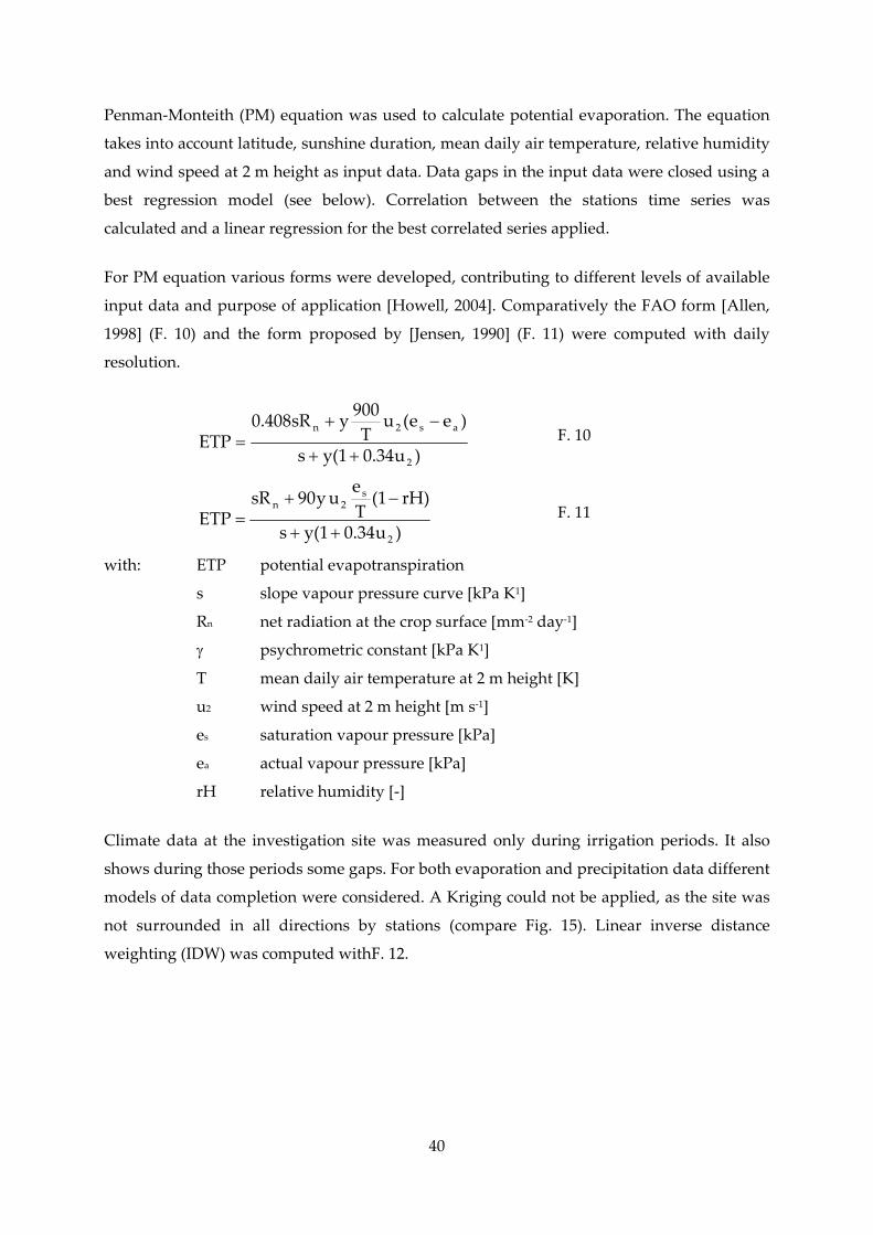
Penman‐Monteith (PM) equation was used to calculate potential evaporation. The equation
takes into account latitude, sunshine duration, mean daily air temperature, relative humidity
and wind speed at 2 m height as input data. Data gaps in the input data were closed using a
best regression model (see below). Correlation between the stations time series was
calculated and a linear regression for the best correlated series applied.
For PM equation various forms were developed, contributing to different levels of available
input data and purpose of application [Howell, 2004]. Comparatively the FAO form [Allen,
1998] (F. 10) and the form proposed by [Jensen, 1990] (F. 11) were computed with daily
resolution.
)u34.01(ys
)ee(uT900ysR408.0
ETP2
as2n
++
−+=
)u34.01(ys
)rH1(Teuy90sR
ETP2
s2n
++
−+=
F. 10
F. 11
with: ETP potential evapotranspiration
s slope vapour pressure curve [kPa K1]
Rn net radiation at the crop surface [mm‐2 day‐1]
γ psychrometric constant [kPa K1]
T mean daily air temperature at 2 m height [K]
u2 wind speed at 2 m height [m s‐1]
es saturation vapour pressure [kPa]
ea actual vapour pressure [kPa]
rH relative humidity [‐]
Climate data at the investigation site was measured only during irrigation periods. It also
shows during those periods some gaps. For both evaporation and precipitation data different
models of data completion were considered. A Kriging could not be applied, as the site was
not surrounded in all directions by stations (compare Fig. 15). Linear inverse distance
weighting (IDW) was computed withF. 12.
40

∑∑=n
i i
n
i i
i0 d
1dZ
Z F. 12
with: Z0 interpolated value
Zi value at reference station i
di distance between reference station i and interpolation point
n number of stations considered
IDW does not include information from the interpolation point. In contrast regression
methods set variables from the interpolation point into a relation, e. g. linear regression with
variables from other points. For the study best regression (F. 13) and multiple regression
(MReg) methods (F. 14) were tested and interpolation quality compared. Weighting
coefficients for the MReg were determined with a least squares method.
)n)t(X*m()t(X iBiiA +∨=
n))t(X*m()t(Xi
BiiA += ∑
F. 13
F. 14
with: time series value at station A
time series value at station B (best correlated to A, in order of i)
mi scaling / weighting coefficient
n residual term
)t(XA
)t(X B
2.2.6 Roots and water uptake
[Pregitzer, 1996] describes poplar root systems as wide ranging and extensive. Poplars have
strong horizontal surface roots from which sinker roots develop. In poplar hybrids,
horizontal roots have been measured at 15 m for a 10‐year‐old tree growing in sandy soil and
20 m for an old tree. The development of sinker roots is limited by the level of the water table
or by the soil conditions [Burns, 1990].
According to [Mulia, 2005] roots of poplar explore soil volumes up to 10 m in radius and
more than 3 m in depth. In contrast [Trapp, 2001] mentions that this species roots are
distributed within the upper two meters of the soil layer and 90 % of the roots are found in
the first 60 cm. These rather contrary findings emphasize the flexibility of root systems to
interact with their environment. [Pregitzer, 1996] describes the coarse structural root system
41
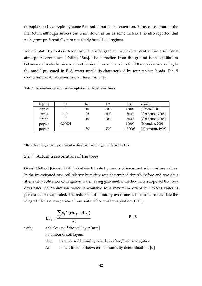
of poplars to have typically some 5 m radial horizontal extension. Roots concentrate in the
first 60 cm although sinkers can reach down as far as some meters. It is also reported that
roots grow preferentially into constantly humid soil regions.
Water uptake by roots is driven by the tension gradient within the plant within a soil plant
atmosphere continuum [Phillip, 1966]. The extraction from the ground is in equilibrium
between soil water tension and root tension. Low soil tensions limit the uptake. According to
the model presented in F. 8, water uptake is characterized by four tension heads. Tab. 5
concludes literature values from different sources.
Tab. 5 Parameters on root water uptake for deciduous trees
h [cm] h1 h2 h3 h4 sourceapple 0 ‐10 ‐1000 ‐15000 [Green, 2003]citrus ‐10 ‐25 ‐400 ‐8000 [Gärdenäs, 2005]grape ‐1 ‐10 ‐1000 ‐8000 [Gärdenäs, 2005]poplar ‐0.00001 ‐10000 [Iskandar, 2001]poplar ‐30 ‐700 ‐13000* [Neumann, 1996]
* the value was given as permanent wilting point of drought resistant poplars
2.2.7 Actual transpiration of the trees
Grassi Method [Grassi, 1978] calculates ET rate by means of measured soil moisture values.
In the investigated case soil relative humidity was determined directly before and two days
after each application of irrigation water, using gravimetric method. It is supposed that two
days after the application water is available to a maximum extent but excess water is
percolated or evaporated. The reduction of humidity over time is then used to calculate the
integral effects of evaporation from soil surface and transpiration (F. 15).
t
)rhrh(*sET i
i,2i,1i
a Δ
−=
∑ F. 15
with: s thickness of the soil layer [mm]
i number of soil layers
rh1/2 relative soil humidity two days after / before irrigation
Δt time difference between soil humidity determinations [d]
42

In agricultural sciences it is common to express actual ET of a crop as ratio to potential ET
with a crop coefficient (kc), e.g. as proposed in [Allen, 1998].
0ca ET*kET = F. 16
with: ETa actual evapotranspiration
kc crop coefficient
The investigation team used two different methods to calculate crop coefficients. On the one
hand the ratio was calculated from pan‐evaporation data on the other hand Blayney‐Criddle
method [Bouwer, 1986] was used to calculate ET in 15 day cycles.
The ratio between actual and potential evaporation of poplar stands depends on water
availability but also on soil conditions. [Verstraeten, 2005] found that actual evaporation
varied about 30% for sites with different soil conditions and similar water yield. Crop
coefficients varied during the growth season between 0.9 and 1.2. Silvicultural grown
poplars under irrigation consume up to 2100 mm/a [Riu, 2004], [Giraud, 2001]. The trees are
resistant and thus often planted under poor water or soil conditions [Zhang, 2005],
[Leguizamón, 2007].
[Chappell, 1997] gives some figures on the transpiration of poplars on a tree‐wise base:
− 100 to 200 l/(d*tree) as optimum transpiration rate for 5 year old trees under different
climatic environments
− 50 l/(d*tree) (estimated annual mean) when trees extract their water directly from the
groundwater table
− up to 40 l/(d*tree) as observed sap flow rates for young hybrid poplars at the
Aberdeen Proving grounds in Maryland
The value determined by [Riu, 2004] for poplars irrigated every seven days corresponds to
an annual mean of 90 l/(d*tree) and is integrating the effects of evaporation and
transpiration.
2.3 Soil properties
Soil samples were taken in a field campaign that was carried out on July 23rd 2008. The
sample distribution was configured in order to retrieve maximum spatial distribution as well
as high representation of the different plant configurations during the growing period.
43
2.3.1 Physical soil properties
To capture the texture properties at first the sedimentation volume (SV) was appraised for all
samples. SV [Nijensohn, 1962a] is a parameter that was developed in Mendoza. It shows
good correlation to clay content and is hence used to estimate soil texture classes. Based on
this, the grading curve was determined for six probes that showed the maximum variation in
SV. 2 mm and 0.5 mm fractions were determined by sieving, finer fractions obtained by
densimetry, as proposed by [ISO 11277, 1998]. Bulk density was determined from
undisturbed samples with a volumetric method [ISO 11272, 1998] and particle density with
picnometer method. Porosity was calculated as ratio of the densities, given by F. 17 and in
comparison from saturated water content (see below) of disturbed samples.
P
B
DD1−=φ F. 17
with: porosity [‐]
DB bulk density [g/cm³]
DP particle density [g/cm³]
φ
Texture classification was derived from three classification standards. The simplest one
refers to SV and was defined by [Nijensohn, 1962a]. ISSS [FAO, 2006] and DIN [DIN 4220,
2007] approaches both take into account grain size distribution.
2.3.2 Water Dynamics
Qualitative rank analysis
In a first step heterogeneity of soil water retention properties was analyzed qualitatively
from variation of soil humidity data. A rank analysis was carried out, as proposed e.g. by
[Ogg, 2000]. Hypothesis was that, if soil properties are spatially heterogeneous, variability
has to be higher between different points of the site than between different dates at the same
point.
As variables of water retention characteristics water content before and after irrigation as
well as water content variation were considered. In order to limit the influence of external
factors (irrigation frequency, climatic conditions in different years) the values were not
analyzed directly but their rank within a group of same external factors, e.g. for all probes
taken in 1991/92 with an irrigation frequency of seven days water contents before irrigation
44

application were compared. The rank was distributed from highest to lowest variable value.
Analysis was carried out for every investigated soil layer separately. The ranks of the
different depths and soil parameters were than averaged over every parcel, this procedure
created the mean rank (F. 18).
∑=d,p
j,ij,i rn1r F. 18
with: j,ir mean rank (specific in time and space)
i control variable of time
j control variable of irrigation regime
p control variable of retention parameter
j control variable of soil depth
j,ir mean rank (specific in time and space)
Variation coefficient (F. 19) was than calculated from the deviation of ranks between
different years (interannual covariation), where measurements have taken place on the same
configuration parcel and irrigation configuration (interconfigurational covariation), where
parcels change and comparison refers to the same year.
)r(mean
)r(SDcov
j,ii
j,iii = F. 19
with: covi interannual variation coefficient
SD standard deviation of ranks
mean arithmetic mean of ranks
The rank parameters mean and SD were than compared with Wilcoxon test of equal
distributions, stating hypothesis F. 20 that the parameters belong to the same distribution.
)ic(p)ia(p:H = F. 20
with: p(ia) probability distribution of interannual ranks
p(ic) probability distribution of interconfigurational ranks
The hypothesis is fulfilled, for the case that testing variable T (F. 21) is higher than z‐quantile
for normal dstributions.
45
)rr(sdev
)r(mean)r(meanT
2,i1,i
2,i1,i
+−
= F. 21
with: p(ia) probability distribution of interannual ranks
p(ic) probability distribution of interconfigurational ranks
Retention properties
Retention curve was determined for suction heads between 5 ‐ 1500 cm; saturated water
content, with 0 cm suction head, with double ring method. At each suction head, water
content was determined gravimetrically. The determinations were carried out for the same
samples, for which grain size distribution were investigated.
Van Genuchten parameters were estimated in two different ways. Physical soil properties
were used to drive two different estimation models and a fitting tool was applied to
measured data. Norm DIN 4220 proposes tabulated values for soil texture classes as given in
[AG Boden, 1994]. ROSETTA software [Schaap, 2000b] was developed by US Soil Salinity
Service (USSS). It implements pedotransfer functions based on artificial neural networks.
Data base for the pedotransfer functions were 2085 soil samples from US territory. Texture
classes, texture distribution, bulk density and single value suction head information can be
incorporated to apply the most exact model possible. Predicted parameters and their
uncertainty ranges are given as output.
In contrast to the estimation approaches presented above, RETC (van Genuchten, 2002) fits
van Genuchten parameters to a given retention curve. It applies a model that fits the
parameters employing a nonlinear least squares optimization approach.
Saturated hydraulic conductivity
Saturated hydraulic conductivity was researched in static pressure head columns under
different pressure heads. The column has a diameter of 2.7 cm and 5 cm height. Pressure
heads were varied between 20 and 50 cm but restricted by the condition that flow rate was
less than two powers higher than permeability [DIN 18130, 1998]. As these experiments are
relatively time consuming, only the four samples that showed maximum variation in
retention properties were considered. Flow rate was measured every 10 – 30 min, with five to
ten repetitions for each pressure head. For statistical validity experiments were repeated 4‐6
times for each soil at different pressure heads.
46
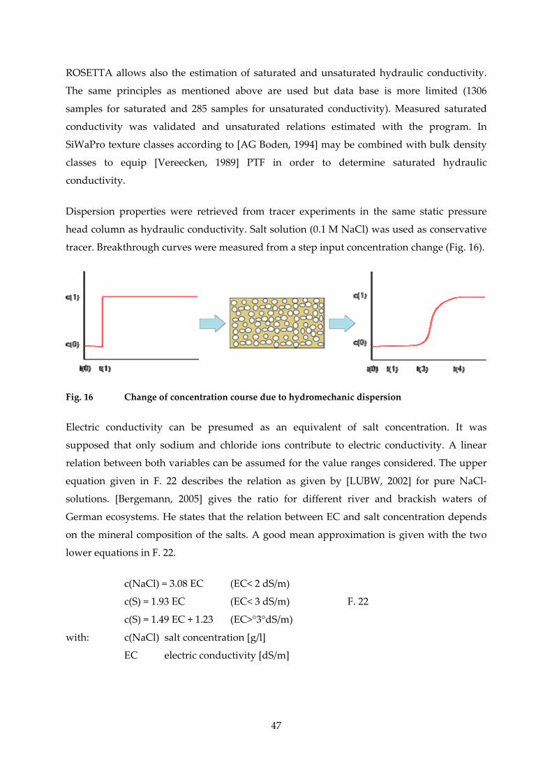
ROSETTA allows also the estimation of saturated and unsaturated hydraulic conductivity.
The same principles as mentioned above are used but data base is more limited (1306
samples for saturated and 285 samples for unsaturated conductivity). Measured saturated
conductivity was validated and unsaturated relations estimated with the program. In
SiWaPro texture classes according to [AG Boden, 1994] may be combined with bulk density
classes to equip [Vereecken, 1989] PTF in order to determine saturated hydraulic
conductivity.
Dispersion properties were retrieved from tracer experiments in the same static pressure
head column as hydraulic conductivity. Salt solution (0.1 M NaCl) was used as conservative
tracer. Breakthrough curves were measured from a step input concentration change (Fig. 16).
Fig. 16 Change of concentration course due to hydromechanic dispersion
Electric conductivity can be presumed as an equivalent of salt concentration. It was
supposed that only sodium and chloride ions contribute to electric conductivity. A linear
relation between both variables can be assumed for the value ranges considered. The upper
equation given in F. 22 describes the relation as given by [LUBW, 2002] for pure NaCl‐
solutions. [Bergemann, 2005] gives the ratio for different river and brackish waters of
German ecosystems. He states that the relation between EC and salt concentration depends
on the mineral composition of the salts. A good mean approximation is given with the two
lower equations in F. 22.
c(NaCl) = 3.08 EC (EC< 2 dS/m)
c(S) = 1.93 EC (EC< 3 dS/m)
c(S) = 1.49 EC + 1.23 (EC>°3°dS/m)
F. 22
with: c(NaCl) salt concentration [g/l]
EC electric conductivity [dS/m]
47

Water density rises with salt concentration and measurement equipment allowed only
determining elevated concentrations. Hence the dispersion experiment was preceded each
time with an upside‐down and downside‐up flow direction, in order to avoid the influence
of density layering due to the experimental setup.
STANMOD toolbox (Simunek, 1998) is applied to retrieve dispersion coefficient from the
measured data using a nonlinear least‐squares parameter optimization method. It is
supposed that salt acts as ideal tracer. For the description of dispersion process equation F.
23 is applied.
xcDI Dc ∂
∂= F. 23
with: Ic mass flux [g/d]
DD dispersivity [m²/d]
2.3.3 Mass Transport
SiWaPro is able to model adsorption and decomposition, therefore a broad variety of
substances can be considered. In the program structure a database for the estimation of
transport properties is implemented. PTFs for mass transport are included take account into
local soil properties. Organic matter, pH‐value and clay content are direct input data for the
deduction of mass transport properties.
Clay content was derived from texture analysis and describes the particle fraction smaller
2 μm. A regression between clay content measured and SV was established. For the soils, for
which only SV was measured, clay content values were interpolated. The pH‐values were
determined in the saturated soil solution. In order to inhibit coagulation of clay minerals,
0.01 M CaCl solution was used to solve to soil. The procedure was applied according to [ISO
10390, 1994]. Loss on ignition method was applied with a combustion temperature of 550°C.
Organic matter content was determined as difference of weight before and after ignition. It
represents a simplified method as described in [DIN 18128, 2002]. The combination of the
three parameters allows giving an appraisal for the transport characteristics of organic and
inorganic substances.
48
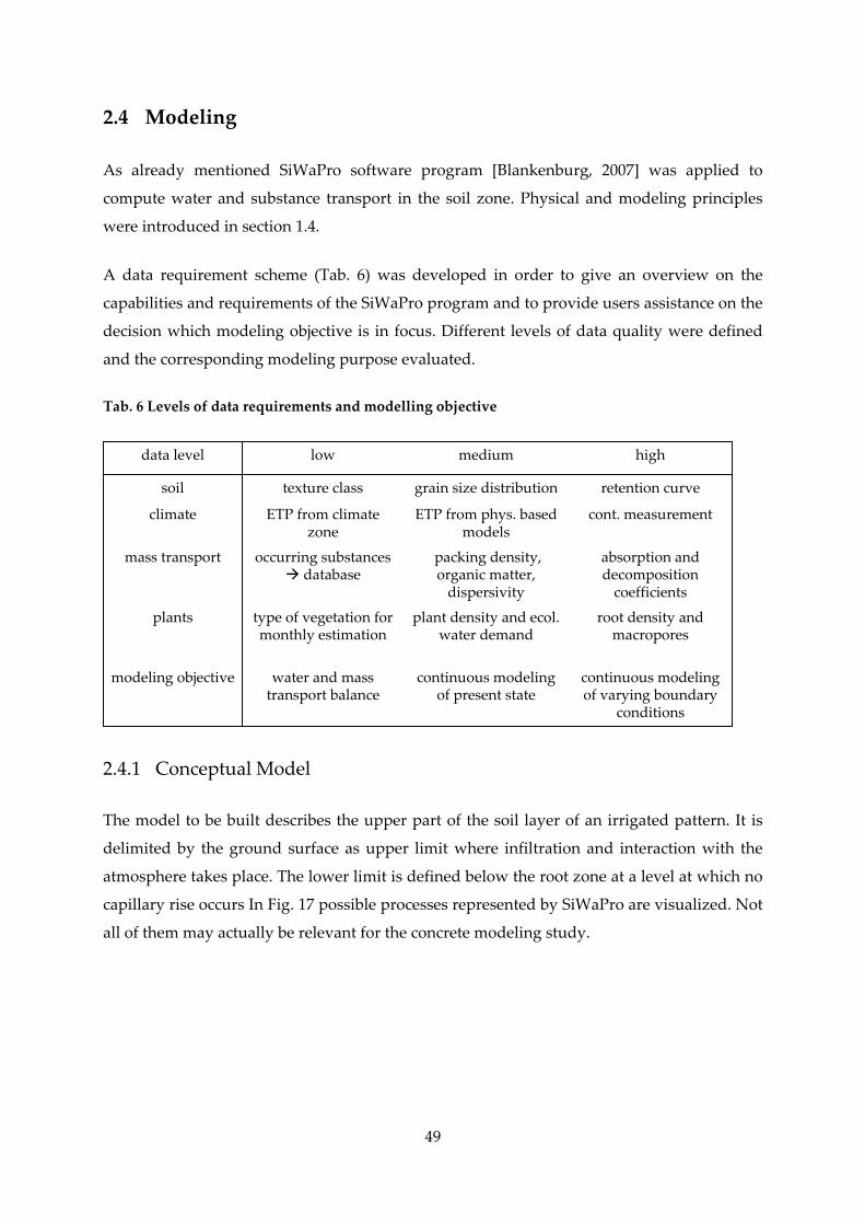
2.4 Modeling
As already mentioned SiWaPro software program [Blankenburg, 2007] was applied to
compute water and substance transport in the soil zone. Physical and modeling principles
were introduced in section 1.4.
A data requirement scheme (Tab. 6) was developed in order to give an overview on the
capabilities and requirements of the SiWaPro program and to provide users assistance on the
decision which modeling objective is in focus. Different levels of data quality were defined
and the corresponding modeling purpose evaluated.
Tab. 6 Levels of data requirements and modelling objective
continuous modeling of varying boundary
conditions
continuous modeling of present state
water and mass transport balance
modeling objective
root density and macropores
plant density and ecol. water demand
type of vegetation for monthly estimation
plants
absorption and decomposition coefficients
packing density, organic matter, dispersivity
occurring substances database
mass transport
cont. measurementETP from phys. based models
ETP from climate zone
climate
retention curvegrain size distributiontexture classsoil
highmediumlowdata level
2.4.1 Conceptual Model
The model to be built describes the upper part of the soil layer of an irrigated pattern. It is
delimited by the ground surface as upper limit where infiltration and interaction with the
atmosphere takes place. The lower limit is defined below the root zone at a level at which no
capillary rise occurs In Fig. 17 possible processes represented by SiWaPro are visualized. Not
all of them may actually be relevant for the concrete modeling study.
49
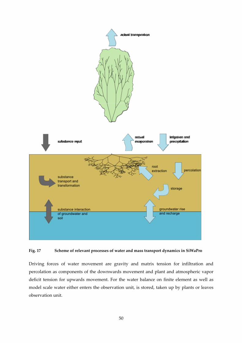
Fig. 17 Scheme of relevant processes of water and mass transport dynamics in SiWaPro
Driving forces of water movement are gravity and matrix tension for infiltration and
percolation as components of the downwards movement and plant and atmospheric vapor
deficit tension for upwards movement. For the water balance on finite element as well as
model scale water either enters the observation unit, is stored, taken up by plants or leaves
observation unit.
50
51
2.4.2 Model Setup
Due to the arrangement of the investigation site, the total area consists of 36 geometrically
equal parcels of 12 x 16 m² (compare Fig. 12). As the program structure only permits a
limited number of equal type boundary conditions (e.g. for water flux at surface under
differing irrigation schemes) parcels were modeled separately.
Resolution
The purpose of the model determines its spatial and temporal resolution. Data availability
suggested a daily resolution of input data. A test of a fourteen day period in a downscaled
hourly resolution was conducted but rejected as generation of input data was laborious and
could only be realized conceptually. With regards to the modelling purpose output did not
differ a lot from results of daily input values.
Several configurations of finite element resolution were tested in order to represent process
dynamics adequately but at the same time guarantee model efficiency and limit computation
time. The configuration finally established was five centimetres mesh size in the upper 30 cm
and a linear vertical increase from 5 – 20 cm between 30 and 200 cm. This resulted in a mesh
of 4091 nodes and 7748 elements.
Model boundaries
Groundwater level is at greater distance from the surface thus it was considered up to which
depth capillary rise might occur. A pre model test was carried out in order to estimate the
height of capillary rise. The test conditions did not take into account the influence of roots.
Soil parameters were adapted for typical loamy sand. Potential gradient is greatest between
saturated conditions and dry surface. To simulate this extreme case, a virtual groundwater
level was lowered 20 cm each time and the model ran for a period of one month without
irrigation or precipitation events. From a depth of groundwater level lower that 1.8 m no
capillary rise was observed (no water flux at surface). Thus it can be assumed, that water that
passes the two meter lower boundary eventually contributes to groundwater recharge.
The lateral component of flow was tested to evaluate in case a significant proportion of water
leave the observation cell that way. For that case the parcel‐wise recognition of the site
would not be adequate. For this pre model boundaries were defined five meters away from
the parcel border. The model was run during one month with four irrigation cycles and three

52
precipitation events. A maximum distribution of wetting front (more than 15 % soil
humidity) outside of the parcel borders was observed. The maximum extension reached
1.5 m, for an irrigation event with shortly antecedent rainfall. It is therefore concluded that
lateral flow is negligible and parcel borders were defined as “no‐flow” boundaries.
Plant configuration
In order to keep the number of calibration parameters on a reasonable level and as
quantifiable information for the site was not available, root distribution and density were
treated conceptually. As described by [Riu, 2008a], already the roots of young poplar trees
reach diameters of more than two meters and are most dense within the uppermost 60 cm.
Literature values were discussed in the review above( section 1.3.3). The layerwise analysis
of [Riu, 1993] indicated, that water extraction was similar in all layers (compare Tab. 11
below) hence all roots were expected to have the same potential of water extraction.
As indicated by [Tschaplinski, 1998] and described in (2.2.6) root distribution develops fairly
independent from irrigation regime, if no severe water stress occurs. It was therefore
assumed that for all trees roots were spread out equally. As root distribution can not be
represented by a time series, it was regarded as stable during the calculation time.
Potential transpiration was obtained by scaling the potential evaporation with the crop
coefficients given in Fig. 23. Uptake scaling parameter was adjusted with the pressure levels
stated by [Neumann, 1996] that are concluded in Tab. 5.
Boundary conditions
The upper boundaries are third type conditions; a climate balance calculated as
precipipitation and irrigation minus evapotranspiration. Time series of flow rates are used
within critical limits: in case water potential head passes an upper or lower threshold, this
value is considered instead. This condition is introduced in order to stabilize computation in
very dry conditions or under water pressure.
The lateral boundaries were described as “no‐flow” condition according to the findings
mentioned above. The lower boundary is defined as a third type condition and represents a
distant groundwater level. Flow is calculated with empirical relation F. 24 that was
introduced by [Hopmans, 1989] for soil water modelling.

)OLh(*Bqh
qheAq −−= F. 24
with: q nodal flow [m²/s]
Aqh scaling factor [m²/s]
Bqh scaling factor [1/m]
h water pressure / tension head [m]
OL surface level [m]
2.5 Representation of present state
In a first step a sensitivity analysis was carried out to enhance system comprehension.
Calibration is conducted based on this knowledge and the experiences from the model setup.
2.5.1 Sensitivity analysis
Starting from the estimated parameters a sensitivity analysis was conducted. The variability
of the input parameters was calculated presuming a normal distribution, as proposed by
[Schaap, 2000b]. Focus of the sensitivity analysis (SA) was to:
− enhance system comprehension
− test the system influences in order to facilitate calibration process
− identify system stability limits in order to avoid model instability
SAs provide a possibility to detect and quantify the relation between input variables, system
parameters and results of a model. Parameters are changed univariantly within sensible
ranges and are set into relation to the response of an output variable.
Parameter ranges
As the model is calibrated with soil moisture data and target variable is the discharge at the
lower model boundary, these two variables were considered in the SA. Van Genuchten
parameters were varied within their normally distributed probability; they were calculated
from the measured values. Boundaries were defined as ten and ninety percent non‐
exceedence probability (quantile).
53
x
z*SDx xq = F. 25
with: xq quantile value of x
q non‐exceedence probability percentile
SDx standard deviation of x
z probability value (tabled) of quantile q for ND
x mean value of x
Execution
The initial “standard” model matched the findings from the model setup routine but without
plants. Soil water content, accumulated discharge and maximum discharge were chosen as
target variables, as they are most representative for system reaction on changes. The model
was run for a period of 30 days with two irrigation pulses at 10 and 20 days. An accumulated
discharge at the lower boundary and water content one meter below surface six days after
irrigation were registered for each parameter combination. The single parameters were
permuted univariantly with the others staying on the standard configuration.
The sensitivity index is a parameter that allows capturing the sensitivity of a target variable
for changes of a certain parameter, if the relation is linear. It describes the increment of one
the target variable over the parameter by differential approximation (F. 26).
SPTV
dSPdTVSI
ΔΔ
≅= F. 26
with: SI sensitivity index
TV target variable
SP system parameter
Nonlinear relations might be described with polynomial or exponential equations [Blair,
2002] but the informative value is much less apparent when compared to the linear
approach.
2.5.2 Calibration and Validation
After model setup calibration is a crucial step to obtain a functional model. In order to fit a
model objectively, optimization needs a measure of agreement between measured data and
simulation results. As already presented for the sensitivity analysis, the basic principle of a
54

calibration is the univariant adaptation of parameters in order to optimize a target function.
Relative humidity was used as target variable. This state variable was measured with high
frequency and is a measure directly related to water dynamics. According to [Riu, 2008a] the
values were examined for each diagnostic layer and at 50 cm distance from a tree. For the
calibration water content values were readout in daily resolution at 6.5 m from the model
border, corresponding to 50 cm distance from the position of the second tree.
Performance parameters
Various measures were tested to assess calibration quality. The formulas in the following are
exemplarily set up for the relative soil humidity that served as calibration target variable.
They serve with some adaptations for many other environmental measures. They are also
used for the evaluation of interpolation quality of input data (sections 3.1.1, 3.1.3). If not
mentioned differently a more detailed description of the indexes can be found in [Willmot,
1985].
The bias describes the difference between mean measured and simulated value. The higher
the difference the less confident is the estimate (F. 27). Bias is applied to detect systematic
differences between measured and simulated data and is base for a further statistical analysis
e. g. of frequency distributions.
2sm )rhrh(bias −= F. 27
with: mrh mean measured relative soil humidity
srh mean simulated relative soil humidity
The bias is integrating the dynamics of measured data so that e. g. differences in the
variability are not captured. This problem is addressed by mean error (ME) based indexes.
The simplest form is given in F. 28.
∑ −=n
isimi )rhrh(
n1ME F. 28
with: ME mean error
n number of observations
rhmi measured relative humidity at date i
rhsi simulated relative humidity at date i
55

A disadvantage of mean error evaluation is that single value deviations of different signs
compensate each other so that the absolute deviation is underestimated. This is avoided by
using the root mean square error (RMSE) as given in F. 29. Absolute values of the single
value deviations are considered and the effect of exceptionally high single deviations is
buffered. Relative root mean square error (rRMSE) is the RMSE divided by mean measured
value. It sets the deviation into a relation with the expectancy index and allows estimating
the magnitude of the error.
∑ −=n
isimi )²rhrh(
n1RMSE
mrh
RMSErRMSE =
F. 29
F. 30
with: RMSE mean error
n number of observations
Nash‐Sutcliffe efficiency (NSE) was introduced by [Nash, 1970] for the evaluation of
hydrologic modeling results (F. 31). Values can range from ‐∞ to 1. An efficiency of 1 (NSE=1)
corresponds to a perfect match of modeled discharge to the observed data. An efficiency of
zero indicates that the model predictions are as accurate as the mean of the observed data,
whereas an efficiency less than zero (‐∞<NSE<0) occurs if the observed mean is a better
predictor than the model.
2
mm
2sm
2mm
)rhrh(
)rhrh()rhrh(NSE
∑ −
∑ −−∑ −= F. 31
with: NSE Nash‐Sutcliffe efficiency
Index of agreement is a measure for the difference between simulation and measured data.
In contrast to standard mean square error based measures it allows additionally to evaluate
relative size of the average difference and is stable for a broad range of comparison data. Big
relative differences in small comparison pairs are considered as strong as those in big
comparison pairs. The IoA can be interpreted as extend with that the simulated values are
able to explain the deviation of measured values. That means the value expresses what
portion of the predictions are error free.
56

2
ssmm
2sm
)rhrhrhrh(
)rhrh(1IoA
∑ −+−
∑ −−= F. 32
with: IoA index of agreement
Correlation coefficient (R) is not a direct index for the evaluation of fitting quality but it is a
measure how strong the dynamic of a variable depends on another. R describes the efficiency
of a predictive function to reproduce a series of data. In its simplest form a linear regression
is used. Coefficient of determination (R²) is the squared correlation coefficient. It can be
interpreted as proportion of the variance of measured data in the variance of the estimation
function. Spearman rank significance test allows the assessment of correlation reliability.
sm rhrh
ssi
n
immi
SD*SD*n
)rhrh()rhrh(R
−−=
∑
F. 33
F. 34
with: R correlation coefficient
standard deviation of measured values
standard deviation of simulated values mrhSD
srhSD
Multi‐objective performance evaluation
The use of multiple parameters causes the problem of a ranking between their importance.
For this work an approach similar to utility analysis is proposed. The method is widely
applied in the field of scenario evaluation in the water management sector [DVWK, 1993]. A
detailed introduction is given in [Eisenführ, 1993]. Adapted on the field of performance
evaluation the idea is to:
− define utility functions for every performance parameter (PP) that scale the
parameter to a value between zero and one
− define weights for the different PPs that scale their contribution to the integral
“performance utility” (PU)
57

∑
∑
=
<<
=
PP
ii
i
PP
iii
1w:and
1)PP(uv0:with
)PP(uv*wPU
F. 35
with: PU performance utility
PP performance parameter
uv(PP) utility value, function of PP
w weighting coefficient
The PU is an integrated parameter that allows the objective evaluation of performance
quality based on multiple evaluation criteria. Weighting coefficients might be defined
according to the prevalent modeling objective and utility functions can be adapted to specific
requirements e. g. as a function of input data quality or significant parameter moments.
2.6 Scenario Setup
Based on the working and calibrated water dynamics model, scenarios of water application
and mass transport are developed. The scenarios try to approach problems of
overexploitation of water and contamination of soil and groundwater due to irrigation.
2.6.1 Salinization due to irrigation
Probably the principle and most widespread source of contamination in Mendoza area is salt
in the irrigation water. Threads and measures were broadly discussed in 1.2.1.
SiWaPro can provide a physically based representation of the unsaturated soil zone. It is thus
a possible link between surface‐ and groundwater compartments and may be used to
validate other more conceptual models.
Motivation
The background and importance of salt as a source of contamination was already introduced
above in sections 1.2.1 and 1.3.2. The idea to set up this scenario was to validate the balance
orientated approaches, e.g. presented by [Mirábile, 2006]. As sodium chloride represents a
conservative constituent the balance is rather easy to draw: the amount of salt that enters is
accumulated in the soil zone or convectively passed to the groundwater. But, as transport
58
59
processes depend on water distribution, the physical based representation allows detecting
distribution patterns and transporting dynamics.
Assumptions
Configuration and boundary conditions are the same as in the calibrated model. Irrigation
water is charged with a conductivity of 1.5 dS/m, corresponding to 0.49 g/l NaCl.
Precipitation water is assumed to not contain any salt. Initial soil conductivity is 2.5 dS/m
corresponding to 0.81 g/l. Irrigation is applied with a seven day frequency and observation
period is one year. Salt is assumed to be a conservative constituent of water, thus neither
adsorption nor decomposition is considered. Dispersion coefficient and dispersivity are
adopted from experiments. The incorporation of salt by the poplars as e.g. mentioned by
[Shannon, 1998] is also neglected.
2.6.2 Irrigation with alternative irrigation methods
Motivation
Basin irrigation is considered as one of the most ineffective methods with regard to water
consumption [FAO, 1995]. Some reasons are:
− water has an extended contact surface with the atmosphere so that evaporation rate is
elevated
− water is distributed equally within the irrigation basin without regard to position of
the plants
− irrigations depths within the field are difficult to control due to surface asperities,
making the method vulnerable to over‐ rather then undersupply of water
Furrow irrigation is another common irrigation method in Mendoza. Generally furrow
irrigation reaches better irrigation efficiencies than basin irrigation [FAO, 1995], which was
also confirmed for Mendoza [Bos, 1997] but application needs more skills and water is
distributed unequal along the furrows. [Schmitz, 2007] proposes a coupled 1D surface – 2D
soil model to describe the flow process along the furrow. Drip irrigation belongs to the micro
irrigation methods that allow providing water adequately in space and time to the plant.
[Riu, 2008b] has done research on the application of drip irrigation for the fertirrigation of
poplars.
60
Assumptions
A cross section profile of the furrow irrigation is considered. The furrows are estimated to
have a contact surface of 0.5 m and trees are situated in the middle of the furrows, as it is
common practice in Mendoza. Irrigation frequency is seven days. Two sub‐cases of irrigation
are considered irrigation with 50 % and 100 % of the water applied in basin irrigation, which
results in irrigation depths of 260 mm or 520 mm respectively within the furrows or 65 mm
or 130 mm per square meter. Over the irrigation season this accumulates to 1300 mm or
2600 mm.
The configuration of the drip irrigation scheme was adapted from [Riu, 2008b]. During the
growth period 48 l/d were applied on every tree corresponding to 320 mm per square meter
in one irrigation season. Two sub‐cases are considered: with and without leaching after the
irrigation season. In the leaching case a pulse of 200 mm is applied on the total irrigation
surface.
As flow processes are supposed to be unaffected by mass transport, salinization is
investigated with the same scenarios.
2.6.3 Phytoremediation of petroleum contamination
Motivation
Just recently a case of uncontrolled petroleum waste disposal was reported for the Piedras
Coloradas oil production [Rojas, 2008] area that affects the investigation site through
downstream El Carrizal reservoir. Various petroleum fields, e.g. at Vicacheras and La
Ventana deposits are found in Rivadavia, the same department as the investigation site. Also
in groundwater wells cases of hydrocarbon contamination were reported in the vicinity of
extraction areas [Rojas, 2003].
Phytoremediation methods are comparatively cheap, accepted by the public and ecologically
advantageous, compared to common technological approaches. The presence of a microflora
in the rhizosphere and the discharge of root exudates [Moormann, 2002] may accelerate the
degradation of contaminants. [Hoffmann, 1998] also mentions the possibility of
incorporation of certain contaminants by certain plants. Furthermore plants have an
influence on the water balance of a site; they change redox potential and pH, and stimulate
microbial activity of the soil [Doty, 2007]. These indirect influences may accelerate

61
degradation in the root zone or reduce the leaching of compounds into the groundwater.
Phytoremediation represents an attractive treatment option for halosols [Ventosa, 2008] and
arid soils [Gómez‐Silva, 2008], where natural activity of micro‐organisms is strongly
reduced.
In spite of the advantages mentioned phytotoxicity and pollutants mass balance have rarely
been documented carefully. Often the success of the projects is not controlled, and only
estimates can be made about the applicability and the potential of Phytoremediation [Trapp,
2000]. Main requirements for further investigation are concluded by [Collins, 2007]:
− species that tolerate the presence‐ or support the degradation of specific pollutants
− reaction of phytoremediation systems on different ages of contamination
− influence and interrelation with environmental boundary conditions
− combination with other treatment options
− possibilities of phytoremediation in ecological restoration
This lack of experience about possibilities and limitations seems to be a hindrance for a
broader use of these techniques. The preliminary modelling of a project allows the effective
design of Phytoremediation, an accompanying control of monitoring results based on the
model supports strategic decisions.
Phytoremediation is an innovative practice for the treatment of petroleum sites. It enhances
the effects of bioremediation especially for potentially toxic petroleum components
[Fiorenza, 1999]. As already introduced above, BTEX are common pollutants in petroleum
contamination. For benzene [Austenat, 1986] gives decomposition half‐lives of 8‐18 months
in soil and up to 4 years in the groundwater. SiWaPro contaminant database gives 720 days
as estimate. Although [BMZ, 1995] mentions that the substance is highly volatile in the upper
soil layer.
Mainly willows, poplars and grasses are applied for the degradation of petroleum products,
aromatic hydrocarbons (BTEX), chlorinated solvents, explosives and cyanides [Frick, 1999].
[Stuwort, 2003] names poplars and alfalfa as most efficient plants for the removal of BTEX
without giving quantifiable information. [Rydberg, 2003] and [Pilipovych, 2006] mention
poplars as suitable crop for the removal of volatile organic carbons. In general, BTEX
compounds are relatively easy to remediate because they are rapidly degraded in the
presence of oxygen, relatively soluble, thus making them bioavailable. Additionally it can
serve as the primary electron donor for many bacteria widely distributed in nature [Frick,
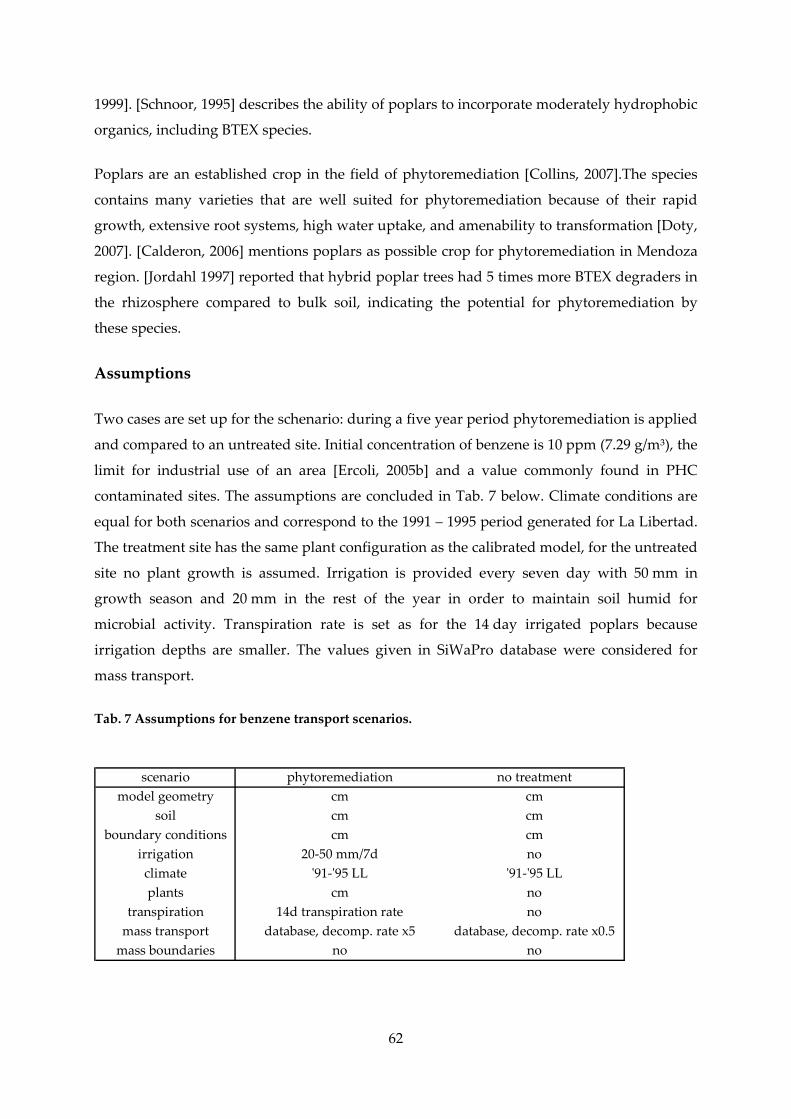
1999]. [Schnoor, 1995] describes the ability of poplars to incorporate moderately hydrophobic
organics, including BTEX species.
Poplars are an established crop in the field of phytoremediation [Collins, 2007].The species
contains many varieties that are well suited for phytoremediation because of their rapid
growth, extensive root systems, high water uptake, and amenability to transformation [Doty,
2007]. [Calderon, 2006] mentions poplars as possible crop for phytoremediation in Mendoza
region. [Jordahl 1997] reported that hybrid poplar trees had 5 times more BTEX degraders in
the rhizosphere compared to bulk soil, indicating the potential for phytoremediation by
these species.
Assumptions
Two cases are set up for the schenario: during a five year period phytoremediation is applied
and compared to an untreated site. Initial concentration of benzene is 10 ppm (7.29 g/m³), the
limit for industrial use of an area [Ercoli, 2005b] and a value commonly found in PHC
contaminated sites. The assumptions are concluded in Tab. 7 below. Climate conditions are
equal for both scenarios and correspond to the 1991 – 1995 period generated for La Libertad.
The treatment site has the same plant configuration as the calibrated model, for the untreated
site no plant growth is assumed. Irrigation is provided every seven day with 50 mm in
growth season and 20 mm in the rest of the year in order to maintain soil humid for
microbial activity. Transpiration rate is set as for the 14 day irrigated poplars because
irrigation depths are smaller. The values given in SiWaPro database were considered for
mass transport.
Tab. 7 Assumptions for benzene transport scenarios.
scenario phytoremediation no treatmentmodel geometry cm cm
soil cm cmboundary conditions cm cm
irrigation 20‐50 mm/7d noclimate ʹ91‐ʹ95 LL ʹ91‐ʹ95 LLplants cm no
transpiration 14d transpiration rate nomass transport database, decomp. rate x5 database, decomp. rate x0.5mass boundaries no no
62
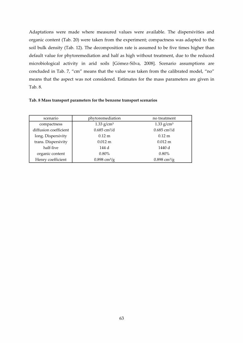
Adaptations were made where measured values were available. The dispersivities and
organic content (Tab. 20) were taken from the experiment; compactness was adapted to the
soil bulk density (Tab. 12). The decomposition rate is assumed to be five times higher than
default value for phytoremediation and half as high without treatment, due to the reduced
microbiological activity in arid soils [Gómez‐Silva, 2008]. Scenario assumptions are
concluded in Tab. 7, “cm” means that the value was taken from the calibrated model, “no”
means that the aspect was not considered. Estimates for the mass parameters are given in
Tab. 8.
Tab. 8 Mass transport parameters for the benzene transport scenarios
scenario phytoremediation no treatmentcompactness 1.33 g/cm³ 1.33 g/cm³
diffusion coefficient 0.685 cm²/d 0.685 cm²/dlong. Dispersivity 0.12 m 0.12 mtrans. Dispersivity 0.012 m 0.012 m
half‐live 144 d 1440 dorganic content 0.80% 0.80%Henry coefficient 0.898 cm³/g 0.898 cm³/g
63

64
3 RESULTS AND DISCUSSION
In the following results of the project are concluded. Special attention is drawn on the part of
input data preparation. To the author this part appears of special interest as data situation in
many arid regions in the world is sparse and efforts have to be focused on the most relevant
factors. As there are not many references available for modeling the vadose zone, this
evaluation might be valuable for future projects. As a consequence the section 3.1 Processing
and evaluation of input data occupies considerable space within the work. As a consequence
soil data section is divided into analysis (3.1.2) and parameter estimation (3.1.3).
3.1 Processing and evaluation of input data
The need and strategy of data enhancement were presented in sections Fehler!
Verweisquelle konnte nicht gefunden werden. to 2.4. In the following results of data
processing are concluded, interpreted and their use in vadose zone modeling is described.
3.1.1 Climate data and plant data
Data consistency
A main drawback of data from the site is that it was only available during the irrigation
periods. Only this time segment was of interest for the antecedent investigation. Hence
reference data for the neighboring stations was obtained and evaporation was calculated in
daily resolution. During the processing of the data some irregularities were identified.
Fig. 18 shows the accumulated tank evaporation data for the measurement period 1991 –
1996. As data was only collected during the irrigation season, corresponding to more or less
120 days per year, the total amount is circa 730 dates. Around the 360th day, corresponding to
January 1994, a clear change in the gradient of the accumulation curve takes place. The
periods before and after this date are approximated satisfyingly with linear trend,
coefficients of determination (R²) are in both cases greater 0.99. Nevertheless gradient slope,
corresponding to mean daily evaporation is reduced after this changing point by more than
half of the initial value, from 8.1 mm/d to 3.9 mm/d.
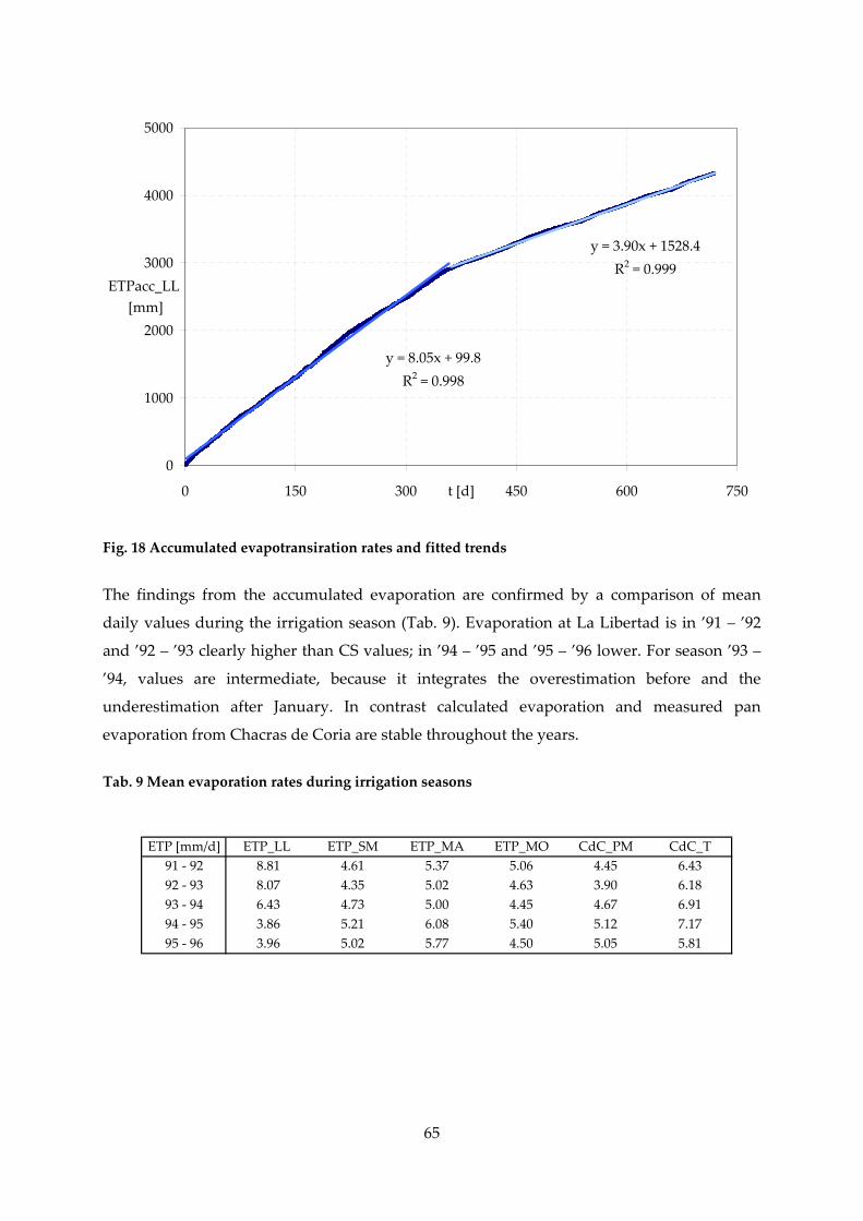
y = 8.05x + 99.8R2 = 0.998
y = 3.90x + 1528.4R2 = 0.999
0
1000
2000
3000
4000
5000
0 150 300 450 600 750t [d]
ETPacc_LL [mm]
Fig. 18 Accumulated evapotransiration rates and fitted trends
The findings from the accumulated evaporation are confirmed by a comparison of mean
daily values during the irrigation season (Tab. 9). Evaporation at La Libertad is in ’91 – ’92
and ’92 – ’93 clearly higher than CS values; in ’94 – ’95 and ’95 – ’96 lower. For season ’93 –
’94, values are intermediate, because it integrates the overestimation before and the
underestimation after January. In contrast calculated evaporation and measured pan
evaporation from Chacras de Coria are stable throughout the years.
Tab. 9 Mean evaporation rates during irrigation seasons
ETP [mm/d] ETP_LL ETP_SM ETP_MA ETP_MO CdC_PM CdC_T91 ‐ 92 8.81 4.61 5.37 5.06 4.45 6.4392 ‐ 93 8.07 4.35 5.02 4.63 3.90 6.1893 ‐ 94 6.43 4.73 5.00 4.45 4.67 6.9194 ‐ 95 3.86 5.21 6.08 5.40 5.12 7.1795 ‐ 96 3.96 5.02 5.77 4.50 5.05 5.81
65

Completition and regionalization of climate data
The time series delivered by SMN consisted of minimum mean and maximum temperature,
relative air humidity, wind speed, sunshine duration and precipitation. The series were not
complete, single dates were missing or not the complete series was available. Missing values
were supplemented by best correlation with other variables from the same station or same
variables from other stations. Correlation was calculated from the existent data. For the best
correlated value the linear regression parameters were determined and the missing value
replaced by the regression estimate.
y = 0.95x + 1.67R2 = 0.989
0
5
10
15
20
25
30
35
0 5 10 15 20 25 30 35
T_av SM [°C]
T_mean SM [°C]
Fig. 19 Correlation between mean temperature and average temperature at San Martin CS
Fig. 19 gives an example for the correlation between mean temperature and the average
value of minimum and maximum temperature value. With a R² of 0.989 the estimation
confidence is high. Regression equation indicates that average value is 1.67°C higher at 0°C
but increases slower with higher mean temperatures, so that for 30°C values are equal.
If no value was available at the best correlated station for the missing date, second, third or
fourth best correlated value were considered. In this way a coherent data set of all stations
was obtained. Statistical analysis showed a convincing completition quality. The difference
66

between mean values was for all stations smaller than one percent, for SD smaller than three
percent.
Comparison on a daily scale between calculated and measured evaporation on a daily
resolution resulted in low accordance. Fig. 20 visualizes that the correlation between single
day values (light blue) is poor, with a R² of 0.2 (significance of 75 %). As a reference: the R²
between Chacras de Coria pan and PM calculated daily values is 0.79 For the five day
moving average the dependence between both variables gets much more apparent, R²
suggests a confidence of correlation with a significance of 95 %.
R2 = 0.668
R2 = 0.206
0
1
2
3
4
5
6
7
0 1 2 3 4 5 6 7ETP_LL [mm/d]
ETP_
SM [m
m/d]
5d mov_av
daily
Fig. 20 Correlation between evaporation from San Martin and La Libertad
If the values of measured and PM evaporation are compared in their temporal course some
additional differences are revealed. In Fig. 21 the courses for precipitation and evaporation at
LL and SM are given for the irrigation season ’93 – ‘94. Light blue lines are from SM dark
blue ones from LL, Fine lines are daily values, bold lines the five day moving average. For
the daily data two aspects are obvious: data from LL shows a much greater variability not
only throughout the whole observation period but also from day to day. This strong
movement could not be related to any other climatic variable from the site or the other CS; it
is thus unclear how it can be explained. The year displayed is the one with the change in
67
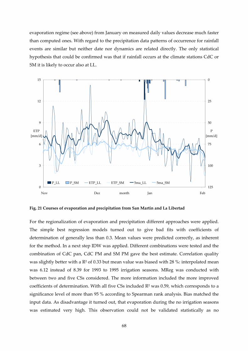
evaporation regime (see above) from January on measured daily values decrease much faster
than computed ones. With regard to the precipitation data patterns of occurrence for rainfall
events are similar but neither date nor dynamics are related directly. The only statistical
hypothesis that could be confirmed was that if rainfall occurs at the climate stations CdC or
SM it is likely to occur also at LL.
0
3
6
9
12
15
Nov Dez Jan Febmonth
ETP [mm/d]
0
25
50
75
100
125
P [mm/d]
P_LL P_SM ETP_LL ETP_SM 5ma_LL 5ma_SM
Fig. 21 Courses of evaporation and precipitation from San Martin and La Libertad
For the regionalization of evaporation and precipitation different approaches were applied.
The simple best regression models turned out to give bad fits with coefficients of
determination of generally less than 0.3. Mean values were predicted correctly, as inherent
for the method. In a next step IDW was applied. Different combinations were tested and the
combination of CdC pan, CdC PM and SM PM gave the best estimate. Correlation quality
was slightly better with a R² of 0.33 but mean value was biased with 28 %: interpolated mean
was 6.12 instead of 8.39 for 1993 to 1995 irrigation seasons. MReg was conducted with
between two and five CSs considered. The more information included the more improved
coefficients of determination. With all five CSs included R² was 0.59, which corresponds to a
significance level of more than 95 % according to Spearman rank analysis. Bias matched the
input data. As disadvantage it turned out, that evaporation during the no irrigation seasons
was estimated very high. This observation could not be validated statistically as no
68

measured data was available but it was judged as unrealistic because none of the observed
stations had values nearly that high. Due to that a combination of IDW and MReg was
chosen. For the irrigation seasons, when measured data was available, it was used for the
estimation of evaporation for the periods of time without reference measured data IDW was
applied SM PM, CdC PM and CdC pan were used as weighting stations. In that way a
coherent, consistent and statistical valid set of evaporation data was generated.
0
4
8
12
16
20
Jun 91 Dez 91 Jun 92 Dez 92 Jun 93 Dez 93 Jun 94 Dez 94 Jun 95 Dez 95
ETP [mm/d]
mess
LL_mreg4
CdC_p
mreg_idw_comb
CdC_PM
Fig. 22 Measured, calculated and interpolated courses of evaporation
In Fig. 22 the comparison of measured data (blue) with CdC PM and pan data (green shades)
and generated time series is given for the whole period during that evaporation data was
available. Bold lines stand for the thirty day moving average, dots represent daily values.
The orange line represents the MReg with four CS series (MO PM, SM PM, CdC PM and
CdC pan). During the irrigation seasons predicted values are acceptable: the general course
is reproduced and the regime change is at least detectable, although not as pronounced as in
the measured data. During winter the evaporation is strongly increased in comparison with
the other courses. Because the fit was optimized with summer data winter values are
overestimated. The red line represents the combined approximation with IDW in non‐
irrigation period (April to October) and MReg with all five CS series during irrigation season
69
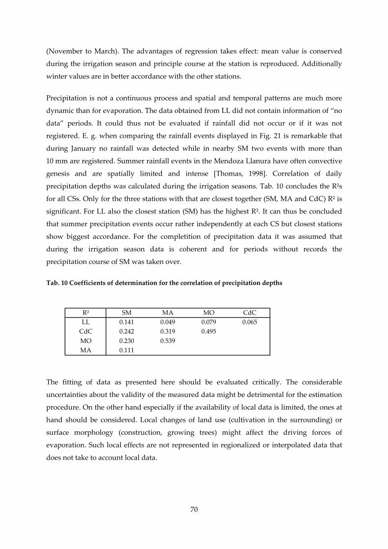
(November to March). The advantages of regression takes effect: mean value is conserved
during the irrigation season and principle course at the station is reproduced. Additionally
winter values are in better accordance with the other stations.
Precipitation is not a continuous process and spatial and temporal patterns are much more
dynamic than for evaporation. The data obtained from LL did not contain information of “no
data” periods. It could thus not be evaluated if rainfall did not occur or if it was not
registered. E. g. when comparing the rainfall events displayed in Fig. 21 is remarkable that
during January no rainfall was detected while in nearby SM two events with more than
10 mm are registered. Summer rainfall events in the Mendoza Llanura have often convective
genesis and are spatially limited and intense [Thomas, 1998]. Correlation of daily
precipitation depths was calculated during the irrigation seasons. Tab. 10 concludes the R²s
for all CSs. Only for the three stations with that are closest together (SM, MA and CdC) R² is
significant. For LL also the closest station (SM) has the highest R². It can thus be concluded
that summer precipitation events occur rather independently at each CS but closest stations
show biggest accordance. For the completition of precipitation data it was assumed that
during the irrigation season data is coherent and for periods without records the
precipitation course of SM was taken over.
Tab. 10 Coefficients of determination for the correlation of precipitation depths
R² SM MA MO CdCLL 0.141 0.049 0.079 0.065CdC 0.242 0.319 0.495MO 0.230 0.539MA 0.111
The fitting of data as presented here should be evaluated critically. The considerable
uncertainties about the validity of the measured data might be detrimental for the estimation
procedure. On the other hand especially if the availability of local data is limited, the ones at
hand should be considered. Local changes of land use (cultivation in the surrounding) or
surface morphology (construction, growing trees) might affect the driving forces of
evaporation. Such local effects are not represented in regionalized or interpolated data that
does not take to account local data.
70

Plant water uptake and actual evapotranspiration
As already mentioned for plant water consumption no additional investigations were
undertaken. Assumptions rely on the results obtained in the previous project. The analysis
presented in this section are based on unpublished [Riu, 1993] and published [Riu, 2003],
[Riu, 2004] data.
Tab. 11 Actual water consumption (transpiration) from different soil depths
layer 0‐30 cm 30‐60 cm 60‐90 cm 90‐120 cm totalT (6 y, 21d) [mm] 236.7 216.0 164.7 170.1 788rel. T (6y, 21d) [%] 30.1 27.4 20.9 21.6T (6y, 14d) [mm] 343.8 295.2 313.2 269.1 1221rel. T (6y, 14d) [%] 28.2 24.2 25.6 22.0T (6y, 7d) [mm] 521.1 438.3 472.5 557.1 1989rel. T (6y, 7d) [%] 26.2 22.0 23.8 28.0mean rel. T 28.1 24.5 23.4 23.9
From the pedological point of view transpiration can be seen as a sink for water in the soil
zone. Applying Grassi Method (compare F. 15) water consumption in the soil was calculated.
The results are concluded in Tab. 11 as integrated annual (irrigation seasonal) values in an
average of the three subsequent irrigation seasons 1991 to 1994. For six year poplars water
consumption depends largely on irrigation frequency. Poplars irrigated every 21 days (first
two lines) consume 788 mm annually, less than half of the water consumed by poplars
irrigated every week (last two lines). With respect to the consumption per soil horizon it
appears that uptake is distributed rather equal over the whole diagnostic depth. Roughly
25 % of the total consumption takes place in the four layers investigated. For the 14 day and
21 day irrigated trees consumption in the upper layers is slightly higher than in the lower
layers. For the seven day irrigated trees uppermost and deepest layer consume most. It can’t
be excluded that this might be related to deep percolation from this zone or different
retention properties in the lower part (compare section 3.1.2 below).
The kc is the actual evapotranspiration normalized over the potential evapotranspiration. For
the antecedent irrigation project actual evaporation and kc’s were calculated for a reference
period of 15 days. The potential ET was taken from pan values and comparatively calculated
with Blayney‐Criddle (BC) method. The average results for irrigation seasons 1991 – 1994 are
concluded in Fig. 23 below. The sections on the x‐axis refer to one of these reference periods
71

each. It is noticeable that the course of kc’s is strongly determined by the course of the actual
ET, this indicates that potential ET is fairly stable over this period of time. The values
themselves and differences between BC and pan based kc’s are bigger for higher irrigation
frequencies and also the seasonal course is more pronounced. The peak in November can be
interpreted as elevated consumption in the sprouting phase and the peak in February as
period of maximum energy incorporation.
0
1
2
3
4
5
Nov Nov Dez Dez Jan Jan Feb Feb Mrz
kc
0
5
10
15
20
25
ETa [mm/d]
kc(pan)_7d kc(pan)_14d kc(pan)_21dkc(BC)_7d kc(BC)_14d kc(BC)_21dETa_7d ETa_14d ETa_21d
Fig. 23Actual evapotranspiration and crop coefficients for six year poplars
3.1.2 Soil data analysis
Special attention was spent on soil data evaluation. The initial research of the irrigation –
growth project indicated that soil was quite homogeneous and visual appraisal on site
seemed to confirm this. Nevertheless, as La Libertad is situated at the border of genetically
different soils (Fig. 10) and surrounding is highly variable considering salinization and
potential vegetation, it seemed valuable to gather more detailed information. Hence a
sampling campaign was carried out on July 23rd 2008. Soil was sampled at six points and at
each point in four depths. The points and extensions of the investigation site were geo‐
72

referenced with a GPS handheld. Distribution of sampling points and configuration of the
site is displayed in Fig. 24
Fig. 24 Georeferenced distribution of sample points
Physical soil properties
The understanding and evaluation of water movement in the subsurface is directly based on
a proper estimation of soil properties, they indicate evolution, behavior and threads of a soil.
With respect to modeling, soil parameters can be divided into three groups: porosity is a
direct input parameter that drives model equations. Bulk density and grain size distribution
are used to equip sub‐models to parameterize retention models. Finally particle density and
sedimentation volume are applied in “sub‐sub‐models” (section 2.3.2) to estimate other soil
properties as the ones mentioned above.
73

Tab. 12 Bulk densities at different sample points and sample layers
Bulk density [g/cm³]MP mean MP SD MP depth mean depth SD depth1 1.32 0.07 0 ‐ 30 cm 1.39 0.062 1.39 0.10 30 ‐ 60 cm 1.37 0.043 1.38 0.13 60 ‐ 90 cm 1.34 0.044 1.38 0.15 90 ‐ 150 cm 1.39 0.095 1.37 0.016 1.37 0.13
mean 1.37 0.10 mean 1.37 0.06SD 0.02 SD 0.02VC 0.02 VC 0.02
Bulk density describes the ratio of weight to volume of an undisturbed soil package. The
parameter could be determined for 20 of the soil sample, the other four showed problems
during sampling procedure. In Tab. 12 comparison of bulk density values is displayed for
the different sample points and diagnostic layers. For both comparison dimensions values
are pretty homogeneous and don’t show trends in direction or with depth. SDs are higher for
sample points than for depth comparison, indicating that soils layers are more
heterogeneous than locations.
Tab. 13 Particle densities at different sample points and sample layers
Particle density [g/cm³]MP mean MP SD MP depth mean depth SD depth1 2.61 0.15 0 ‐ 30 cm 2.54 0.102 2.60 0.08 30 ‐ 60 cm 2.62 0.043 2.64 0.08 60 ‐ 90 cm 2.63 0.064 2.66 0.04 90 ‐ 150 cm 2.69 0.035 2.60 0.086 2.63 0.06
mean 2.62 0.08 mean 2.62 0.06SD 0.02 SD 0.06VC 0.01 VC 0.02
Particle density describes the specific weight of grains that make up the soil. Values were
determined for the complete population of 24 samples. Tab. 13 shows the values of particle
density in a comparison along the different sample sites and sample layers. Generally values
are rather high, quartz soils commonly have particle densities around 2.4 g/cm³. This might
74
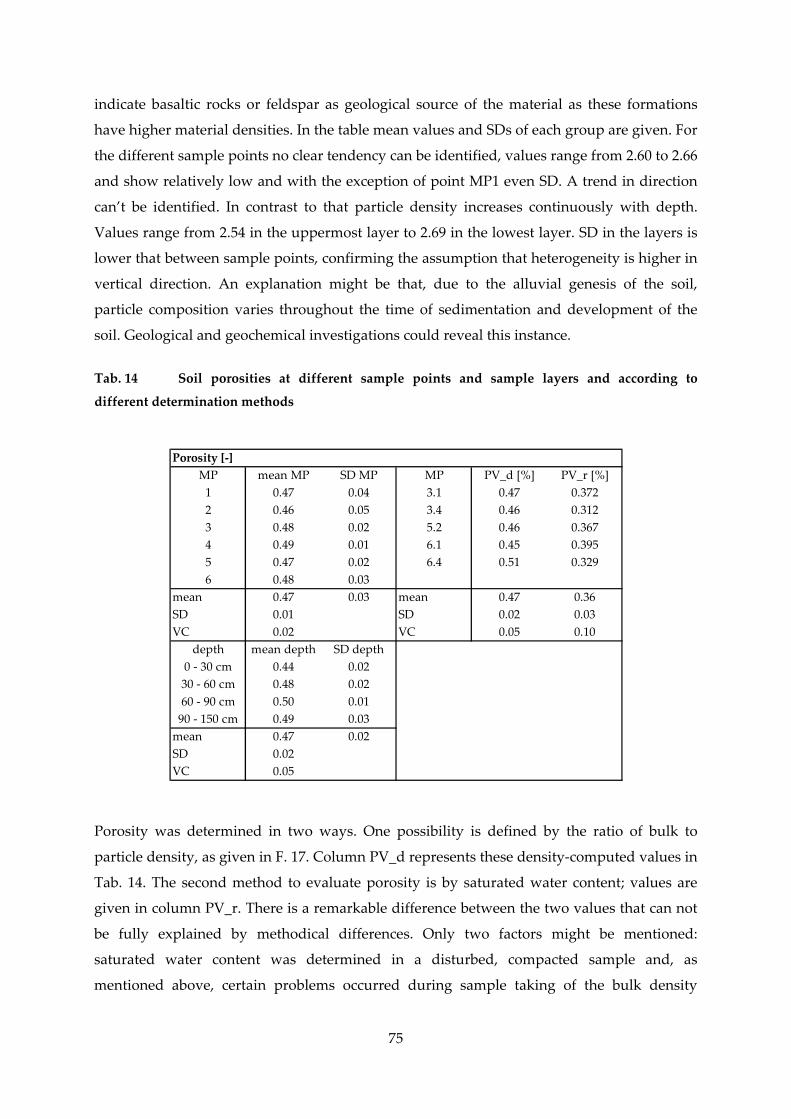
indicate basaltic rocks or feldspar as geological source of the material as these formations
have higher material densities. In the table mean values and SDs of each group are given. For
the different sample points no clear tendency can be identified, values range from 2.60 to 2.66
and show relatively low and with the exception of point MP1 even SD. A trend in direction
can’t be identified. In contrast to that particle density increases continuously with depth.
Values range from 2.54 in the uppermost layer to 2.69 in the lowest layer. SD in the layers is
lower that between sample points, confirming the assumption that heterogeneity is higher in
vertical direction. An explanation might be that, due to the alluvial genesis of the soil,
particle composition varies throughout the time of sedimentation and development of the
soil. Geological and geochemical investigations could reveal this instance.
Tab. 14 Soil porosities at different sample points and sample layers and according to
different determination methods
Porosity [‐]MP mean MP SD MP MP PV_d [%] PV_r [%]1 0.47 0.04 3.1 0.47 0.3722 0.46 0.05 3.4 0.46 0.3123 0.48 0.02 5.2 0.46 0.3674 0.49 0.01 6.1 0.45 0.3955 0.47 0.02 6.4 0.51 0.3296 0.48 0.03
mean 0.47 0.03 mean 0.47 0.36SD 0.01 SD 0.02 0.03VC 0.02 VC 0.05 0.10
depth mean depth SD depth0 ‐ 30 cm 0.44 0.0230 ‐ 60 cm 0.48 0.0260 ‐ 90 cm 0.50 0.0190 ‐ 150 cm 0.49 0.03mean 0.47 0.02SD 0.02VC 0.05
Porosity was determined in two ways. One possibility is defined by the ratio of bulk to
particle density, as given in F. 17. Column PV_d represents these density‐computed values in
Tab. 14. The second method to evaluate porosity is by saturated water content; values are
given in column PV_r. There is a remarkable difference between the two values that can not
be fully explained by methodical differences. Only two factors might be mentioned:
saturated water content was determined in a disturbed, compacted sample and, as
mentioned above, certain problems occurred during sample taking of the bulk density
75

samples. The PV_d values are very high and uncommon for soils with a low organic content
in contrast PV_r values are to low for most soils. For loamy sands, the group to which the
soils belong according to a first visual estimation, porosities typically range around 0.4.
Tab. 15 Sedimentation volumes at different sample points and sample layers
Sedimentation volume [ml/100g]MP mean MP SD MP depth mean depth SD depth1 89 2.00 0 ‐ 30 cm 92 6.202 88 4.12 30 ‐ 60 cm 85 6.533 78 5.16 60 ‐ 90 cm 86 3.674 84 8.00 90 ‐ 150 cm 81 6.535 88 8.646 91 3.83
mean 86.25 5.29 mean 86.25 5.73SD 4.64 SD 4.40VC 0.05 VC 0.05
Sedimentation volume is a parameter that allows estimation of texture properties.
[Nijensohn, 1962b] states a strong correlation between clay content and SV. In Mendoza it is
used for a general texture classification. For the project all samples were analyzed, mainly to
identify most heterogeneous samples for a more detailed view. SVs vary considerably
between the different sample points. Lowest mean values occur for the central sample points
“3” and “4”. No tendencies can be identified for a change with direction. Mean values of SV
augment with smaller distance to surface, indicating that material gets sandier in deeper
layers. This finding may correspond to different soil composition as described for particle
density. Absolute highest SV amounts to 96, it occurs at point six in the uppermost layer. The
lowest value was examined for the lowest layer of point 3.
Grain size distributions (Fig. 25) were determined for the six soils that showed biggest
variability in SV, namely 2‐4, 3‐1, 3‐4, 5‐2, 6‐1 and 6‐4. Hence all sample points, aside from
MP1 and all depths aside from 75 cm were considered. All soils examined show the whole
range of texture classes. Skeletal fraction accounted in all samples with less than 1 %, hence
soil can be defined as stone free. Biggest variation between the samples results for silt
fraction, between 0.01 ‐ 0.1 mm. In clay and silt fractions soils 6‐1 as finest and 3‐4 as coarsest
soil define the ranges. This corresponds to the findings of SV determination 6‐1 ranged
highest and 3‐4 lowest. For medium sand fraction and coarser soils 6‐4 and 2‐4 are limiting.
76

Fig. 25 Grain size distribution of six soils at the investigation site
Texture properties are concluded in Tab. 16. Texture class portions refer to the texture class
ranges as defined by [AG Boden, 1994]. Sand and silt represent are biggest fractions of all
soils with portions roughly between 30 – 60 %. Absolute variance is most pronounced for
sand, where fraction ranges between 34 – 68 %. Clay shows highest relative variability but
absolute fractions are generally lowest (2 – 10 %). For classification, texture ranges were
applied as proposed by US Natural Recourses Conversation Service (NRSC) [USDA, 1999]
and by Manual of Soil Mapping (KA4, Bodenkundliche Kartieranleitung) [AG Boden, 1994]
respectively. According to NRSC soils are sandy loams (Ls), loams (L) and silty loams (Lu).
While KA4 classifies medium silty sand (Su3), very silty sand (Su4), loamy silty sand (Slu)
and loamy sandy silt (Uls). SV categories, as defined in [Nijensohn, 1962a] correspond fairly
to KA4 classification, especially as silt is not considered separately from loam, soils are
identified as sand, loamy sand and loam. Nevertheless texture categories are coarser than
NRSC and KA4 categories. Generally NRSC gives classifications with a shift towards finer
soils.
77
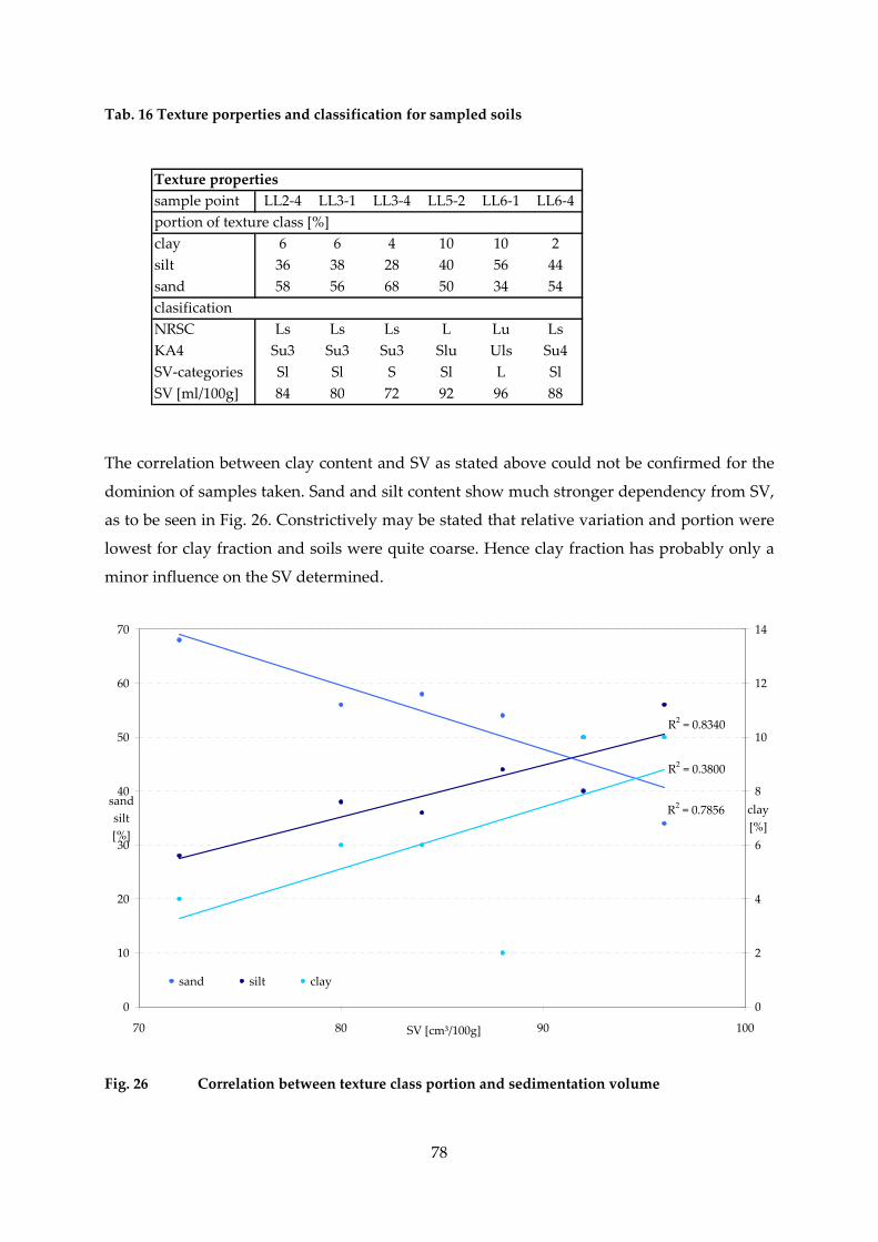
Tab. 16 Texture porperties and classification for sampled soils
Texture propertiessample point LL2‐4 LL3‐1 LL3‐4 LL5‐2 LL6‐1 LL6‐4portion of texture class [%]clay 6 6 4 10 10 2silt 36 38 28 40 56 44sand 58 56 68 50 34 54clasificationNRSC Ls Ls Ls L Lu LsKA4 Su3 Su3 Su3 Slu Uls Su4SV‐categories Sl Sl S Sl L SlSV [ml/100g] 84 80 72 92 96 88
The correlation between clay content and SV as stated above could not be confirmed for the
dominion of samples taken. Sand and silt content show much stronger dependency from SV,
as to be seen in Fig. 26. Constrictively may be stated that relative variation and portion were
lowest for clay fraction and soils were quite coarse. Hence clay fraction has probably only a
minor influence on the SV determined.
R2 = 0.7856
R2 = 0.8340
R2 = 0.3800
0
10
20
30
40
50
60
70
70 80 90 100SV [cm³/100g]
sandsilt[%]
0
2
4
6
8
10
12
14
clay[%]
sand silt clay
Fig. 26 Correlation between texture class portion and sedimentation volume
78

Interpolation of soil properties
In order to discover patterns in the distribution of the soil properties grids were interpolated
applying a linear Kriging method. Grids were generated for each sampling layer, and three
cross sections, as given in Fig. 27. The actual sample points can be seen in Fig. 13. The lines
within the map mark position of the cross sections, they correspond to northing coordinates
6321700 and 6321800 and easting coordinate 2546900. Interpolation was carried out in a 5 m
resolution. The coordinates refer to the Universal Transverse Mercator projection.
Fig. 27 Position of the cross sections (lines) for the interpolation of soil properties
In Fig. 28 four maps of the sedimentation volume are given. The layers are arranged as
0.15 mbsl upper left, 0.45 mbsl upper right, 0.75 mbsl lower left and 1.20 mbsl lower right.
The findings from the statistical analysis (Tab. 15) are confirmed, SV decreases with depth,
indicating more pervious soil in deeper layers. Additionally the horizontal distribution of the
values can be captured easily. Generally SVs are higher in the eastern (right) part of the area.
A bay of material with lower SVs enters the site from the west; this material bay seems to
expand with depth, with the only exception at 75 cm below surface. The material in the
79
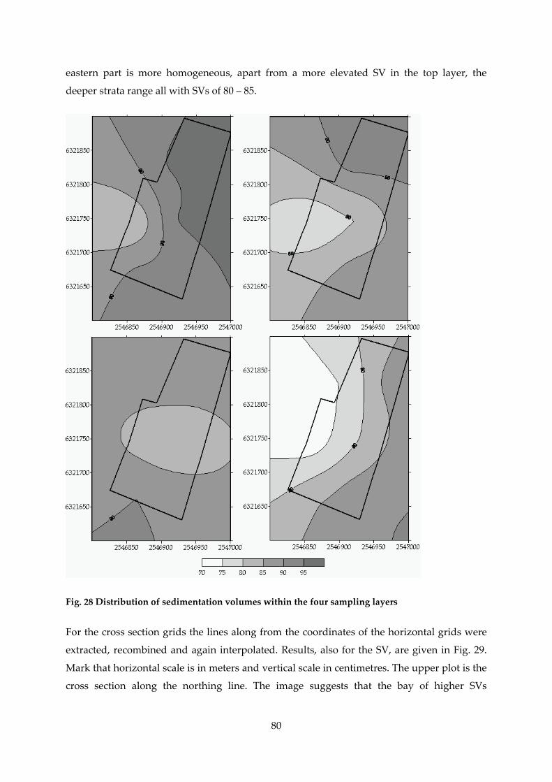
eastern part is more homogeneous, apart from a more elevated SV in the top layer, the
deeper strata range all with SVs of 80 – 85.
Fig. 28 Distribution of sedimentation volumes within the four sampling layers
For the cross section grids the lines along from the coordinates of the horizontal grids were
extracted, recombined and again interpolated. Results, also for the SV, are given in Fig. 29.
Mark that horizontal scale is in meters and vertical scale in centimetres. The upper plot is the
cross section along the northing line. The image suggests that the bay of higher SVs
80

identified above is more pronounced in the northern part of the area (right) while in the
southern part the profile is more homogeneous. The two lower images are the cross sections
along the easting lines. They support the finding of the bay in the West of the area. The more
homogeneous profiles in the East are also confirmed.
Fig. 29 Distribution of sedimentation volumes along three cross sections
Hydraulic properties
Retention curves were determined at INTA (Instituto Nacional de Tecnología Agropecuaria)
laboratories. The water content – suction head relation was measured for saturated condition
and six suction heads, at 5, 10, 30, 100, 300 and 1500 cm WC. Fig. 30 shows measured data in
green shades and estimates of two prediction models (ROSETTA, DIN4220) and a fitting
model (RETC) are given in blue shades. Axis of ordinates shows pF value, that represents the
decadal logarithm of suction head. As in the experiments above, soils 3.4 and 6.1 define the
range of values, with approximately 10% difference in water content for equal suction heads.
On the other hand for the range of suction heads considered same water contents correspond
81

to differences in suction head of more than 1000 cm WC. Soil 6.1, that has the finest texture
stores highest water contents, while coarsest soil 3.4 stores fewest water. Generally measured
curves progress flatter that prediction curves, corresponding to higher loss of water with
increasing suction head, the effect will be discussed in 3.1.3, further below.
0.0
0.5
1.0
1.5
2.0
2.5
3.0
3.5
4.0
4.5
0.00 0.05 0.10 0.15 0.20 0.25 0.30 0.35 0.40 0.45wc [‐]
pF
rosetta DIN4220 RETC
LL 3‐1 LL‐3.4 LL‐5.2
LL‐6.1 LL‐6.4 LL 2‐4
Fig. 30 Measured retention curves in comparison to estimation models
Saturated hydraulic conductivity was determined in laboratory with disturbed soil samples
of sample points 3.1, 3.4, 5.2 and 6.4 in a constant head column. Experiments were repeated
four to six times with different pressure heads. The values for the repetitions are given in
Tab. 17. They represent the average of seven to ten realizations obtained under equal
pressure heads. From the average of the realizations, the average of the repetitions was
calculated. Additionally SD and variation coefficient of repetitions allow estimating the
uncertainty of the determination procedure. Soil 3.4 shows highest conductivity, it is with
5.96 E‐06 m/s about eight times higher than soil 6.4’s conductivity that has the lowest value
with 7.23 E‐07 m/s. Hence the same soils as in the previous experiments defined the range of
occurring values. The conductivities of soils 3.1 and 5.2 rank between the extremes with
values between 1 E‐06 m/s and 2 E‐06 m/s. The SDs are generally more than one order of
82
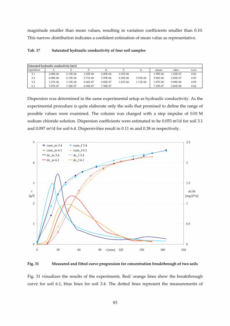
magnitude smaller than mean values, resulting in variation coefficients smaller than 0.10.
This narrow distribution indicates a confident estimation of mean value as representative.
Tab. 17 Saturated hydraulic conductivity of four soil samples
Saturated hydraulic conductivity [m/s]repetition 1. 2. 3. 4. 5. 6. mean sdev vcov 3.1 2.08E‐06 2.13E‐06 1.83E‐06 2.00E‐06 1.91E‐06 1.99E‐06 1.20E‐07 0.06 3.4 6.08E‐06 6.15E‐06 5.71E‐06 5.59E‐06 6.34E‐06 5.91E‐06 5.96E‐06 2.82E‐07 0.05 5.2 1.21E‐06 1.13E‐06 9.66E‐07 9.82E‐07 1.01E‐06 1.11E‐06 1.07E‐06 9.98E‐08 0.09 6.1 7.07E‐07 7.34E‐07 6.94E‐07 7.58E‐07 7.23E‐07 2.86E‐08 0.04
Dispersion was determined in the same experimental setup as hydraulic conductivity. As the
experimental procedure is quite elaborate only the soils that promised to define the range of
possible values were examined. The column was charged with a step impulse of 0.01 M
sodium chloride solution. Dispersion coefficients were estimated to be 0.053 m²/d for soil 3.1
and 0.097 m²/d for soil 6.4. Dispersivities result in 0.11 m and 0.38 m respectively.
0
1
2
3
4
5
0 30 60 90 120 150 180 210t [min]
c[g/l]
0
0.5
1
1.5
2
2.5
dc/dt[mg/(l*s)]
cum_m 3.4 cum_f 3.4cum_m 6.1 cum_f 6.1dc_m 3.4 dc_f 3.4dc_m 6.1 dc_f 6.1
Fig. 31 Measured and fitted curve progression for concentration breakthrough of two soils
Fig. 31 visualizes the results of the experiments. Red/ orange lines show the breakthrough
curve for soil 6.1, blue lines for soil 3.4. The dotted lines represent the measurements of
83
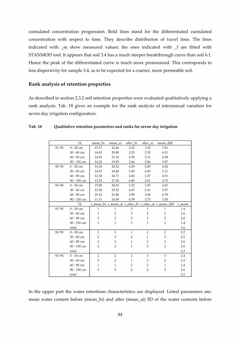
cumulated concentration progression. Bold lines stand for the differentiated cumulated
concentration with respect to time. They describe distribution of travel time. The lines
indicated with _m show measured values; the ones indicated with _f are fitted with
STANMOD tool. It appears that soil 3.4 has a much steeper breakthrough curve than soil 6.1.
Hence the peak of the differentiated curve is much more pronounced. This corresponds to
less dispersivity for sample 3.4, as to be expected for a coarser, more permeable soil.
Rank analysis of retention properties
As described in section 2.3.2 soil retention properties were evaluated qualitatively applying a
rank analysis. Tab. 18 gives an example for the rank analysis of interannual variation for
seven day irrigation configuration.
Tab. 18 Qualitative retention parameters and ranks for seven day irrigation
7d mean_bi mean_ai sdev_bi sdev_ai mean_diff91‐ʹ92 0 ‐ 30 cm 15.17 22.46 2.52 3.32 7.81
30 ‐ 60 cm 14.63 20.80 2.25 2.52 6.5160 ‐ 90 cm 14.93 21.10 2.39 3.11 6.3890 ‐ 150 cm 14.52 19.83 2.66 5.06 5.97
92‐ʹ93 0 ‐ 30 cm 14.34 20.32 4.29 2.85 6.0230 ‐ 60 cm 14.33 18.40 3.84 4.83 5.1160 ‐ 90 cm 12.30 16.71 4.02 2.27 4.5190 ‐ 150 cm 13.25 17.29 6.00 2.61 5.75
93‐ʹ94 0 ‐ 30 cm 15.08 20.65 3.32 1.93 6.0130 ‐ 60 cm 13.38 18.52 4.03 2.41 5.9760 ‐ 90 cm 15.12 21.80 3.99 3.04 6.7890 ‐ 150 cm 11.11 14.59 4.39 3.73 5.30
7d r_mean_bi r_mean_ai r_sdev_bi r_sdev_ai r_mean_diff r_mean91‐ʹ92 0 ‐ 30 cm 1 1 3 1 1 1.4
30 ‐ 60 cm 1 1 3 2 1 1.660 ‐ 90 cm 2 2 3 1 2 2.090 ‐ 150 cm 1 1 3 1 1 1.4total 1.6
92‐ʹ93 0 ‐ 30 cm 3 3 1 2 2 2.230 ‐ 60 cm 2 3 2 1 3 2.260 ‐ 90 cm 3 3 1 3 3 2.690 ‐ 150 cm 2 2 1 3 2 2.0total 2.3
93‐ʹ94 0 ‐ 30 cm 2 2 2 3 3 2.430 ‐ 60 cm 3 2 1 3 2 2.260 ‐ 90 cm 1 1 2 2 1 1.490 ‐ 150 cm 3 3 2 2 3 2.6total 2.2
In the upper part the water retentions characteristics are displayed. Listed parameters are:
mean water content before (mean_bi) and after (mean_ai) SD of the water contents before
84
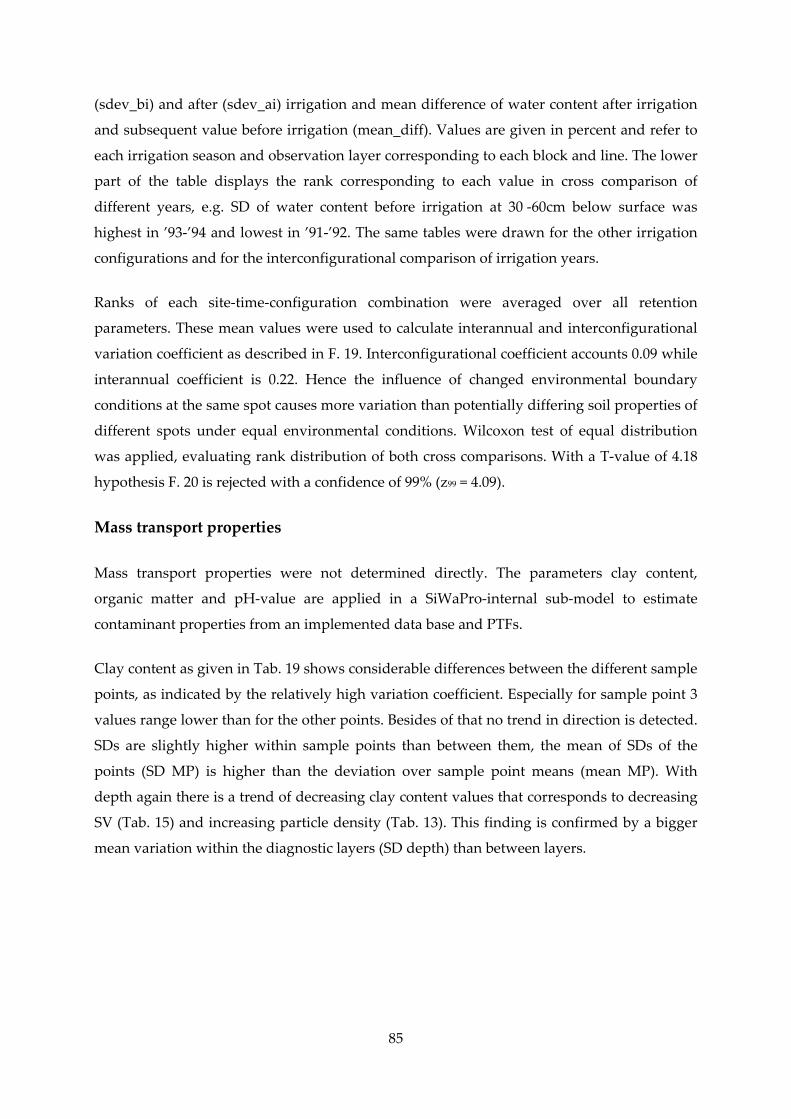
85
(sdev_bi) and after (sdev_ai) irrigation and mean difference of water content after irrigation
and subsequent value before irrigation (mean_diff). Values are given in percent and refer to
each irrigation season and observation layer corresponding to each block and line. The lower
part of the table displays the rank corresponding to each value in cross comparison of
different years, e.g. SD of water content before irrigation at 30 ‐60cm below surface was
highest in ’93‐’94 and lowest in ’91‐’92. The same tables were drawn for the other irrigation
configurations and for the interconfigurational comparison of irrigation years.
Ranks of each site‐time‐configuration combination were averaged over all retention
parameters. These mean values were used to calculate interannual and interconfigurational
variation coefficient as described in F. 19. Interconfigurational coefficient accounts 0.09 while
interannual coefficient is 0.22. Hence the influence of changed environmental boundary
conditions at the same spot causes more variation than potentially differing soil properties of
different spots under equal environmental conditions. Wilcoxon test of equal distribution
was applied, evaluating rank distribution of both cross comparisons. With a T‐value of 4.18
hypothesis F. 20 is rejected with a confidence of 99% (z99 = 4.09).
Mass transport properties
Mass transport properties were not determined directly. The parameters clay content,
organic matter and pH‐value are applied in a SiWaPro‐internal sub‐model to estimate
contaminant properties from an implemented data base and PTFs.
Clay content as given in Tab. 19 shows considerable differences between the different sample
points, as indicated by the relatively high variation coefficient. Especially for sample point 3
values range lower than for the other points. Besides of that no trend in direction is detected.
SDs are slightly higher within sample points than between them, the mean of SDs of the
points (SD MP) is higher than the deviation over sample point means (mean MP). With
depth again there is a trend of decreasing clay content values that corresponds to decreasing
SV (Tab. 15) and increasing particle density (Tab. 13). This finding is confirmed by a bigger
mean variation within the diagnostic layers (SD depth) than between layers.
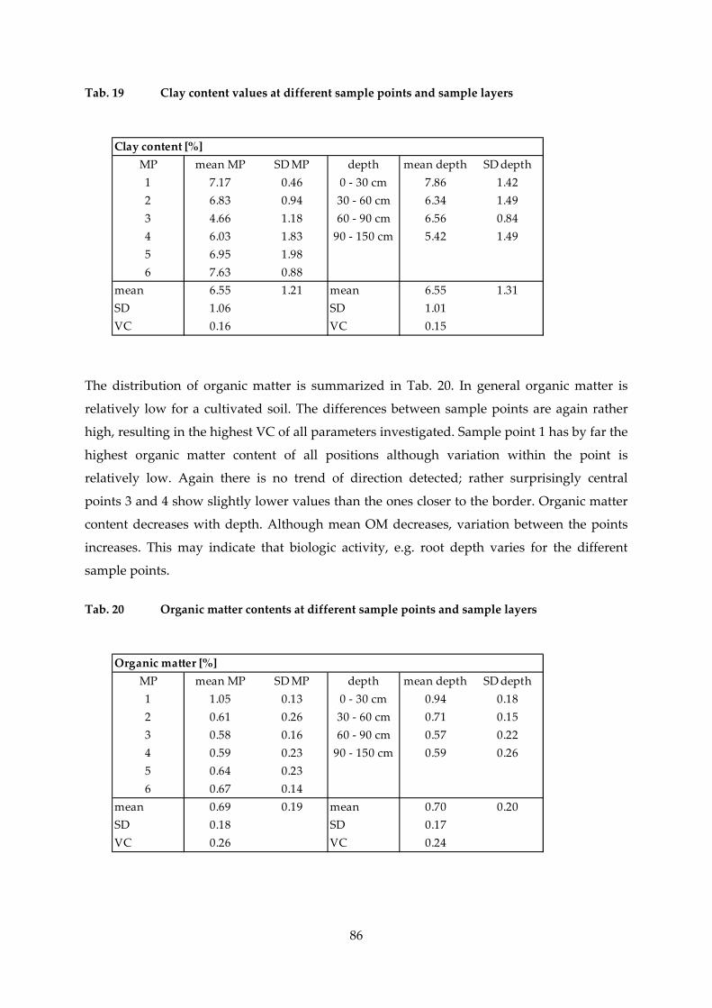
Tab. 19 Clay content values at different sample points and sample layers
Clay content [%]MP mean MP SD MP depth mean depth SD depth1 7.17 0.46 0 ‐ 30 cm 7.86 1.422 6.83 0.94 30 ‐ 60 cm 6.34 1.493 4.66 1.18 60 ‐ 90 cm 6.56 0.844 6.03 1.83 90 ‐ 150 cm 5.42 1.495 6.95 1.986 7.63 0.88
mean 6.55 1.21 mean 6.55 1.31SD 1.06 SD 1.01VC 0.16 VC 0.15
The distribution of organic matter is summarized in Tab. 20. In general organic matter is
relatively low for a cultivated soil. The differences between sample points are again rather
high, resulting in the highest VC of all parameters investigated. Sample point 1 has by far the
highest organic matter content of all positions although variation within the point is
relatively low. Again there is no trend of direction detected; rather surprisingly central
points 3 and 4 show slightly lower values than the ones closer to the border. Organic matter
content decreases with depth. Although mean OM decreases, variation between the points
increases. This may indicate that biologic activity, e.g. root depth varies for the different
sample points.
Tab. 20 Organic matter contents at different sample points and sample layers
Organic matter [%]MP mean MP SD MP depth mean depth SD depth1 1.05 0.13 0 ‐ 30 cm 0.94 0.182 0.61 0.26 30 ‐ 60 cm 0.71 0.153 0.58 0.16 60 ‐ 90 cm 0.57 0.224 0.59 0.23 90 ‐ 150 cm 0.59 0.265 0.64 0.236 0.67 0.14
mean 0.69 0.19 mean 0.70 0.20SD 0.18 SD 0.17VC 0.26 VC 0.24
86

Observed pH values are the measurements with least variation between the different
samples. VC is has lowest values compared to the other measures as well for comparison of
positions as of layers. Sample point 1 has slightly lower values than the other positions and
for all points values increase with depth. But both findings are not significant and below the
range of uncertainty of the measurement.
Tab. 21 pH values at different sample points and sample layers
pHMP mean MP SD MP depth mean depth SD depth1 7.70 0.03 0 ‐ 30 cm 7.79 0.102 7.79 0.08 30 ‐ 60 cm 7.83 0.073 7.89 0.07 60 ‐ 90 cm 7.83 0.074 7.91 0.03 90 ‐ 150 cm 7.88 0.105 7.84 0.066 7.85 0.03
mean 7.83 0.05 mean 7.83 0.09SD 0.08 SD 0.04VC 0.01 VC 0.00
3.1.3 Estimation of soil hydraulic and transport parameters
Retention properties
Fig. 32 shows the estimation quality and probability range for the parameterization with
ROSETTA model. Exemplarily data is given for soil sample 2.4. The colours are arranged
from light to dark blue for increasing input data quality. For each quality level mean (bold
line), minimum and maximum probable ranges (fine lines) are given. The suffix _tex
corresponds to the estimate if only texture class of the soil is given, _SSC for given sand, silt
and clay portions, _SSCBC as before and bulk density and _th1 as before and water content
at field capacity (330 cm WC). Uncertainty ranges get notably smaller with increasing data
quality. If only texture class is known the range for probable water content values under
saturated conditions (pF0) is 0.30 ‐ 0.46, for the best estimation model the range diminishes to
0.33 – 0.37. Nevertheless it gets clear that the measured retention curve is represented badly
by all estimated parameter sets. Especially the fast decrease of water content for low suction
heads can’t be reproduced satisfyingly. Still _th1 allows the closest approximation to the
measured curve. Hence it is indicated to determine at least some characteristic points of the
87

retention curve in order to validate estimation quality and enhance estimation models. An
explanation for the bad estimation quality might be that alluvial soils under arid conditions
of pedogenesis are not very common and hence contribute only to a small part to the domain
that was used to calibrate the pedotransfer functions.
0.0
0.6
1.2
1.8
2.4
3.0
3.6
4.2
0.00 0.14 0.28 0.42 0.56 0.70wc [‐]
pF
ro_tex ro_tex_minro_tex_max ro_SSCro_SSc_min ro_SSC_maxro_SSCBD ro_SSCBD_minro_SSCBD_max ro_th1ro_th1_min ro_th1_maxmess
Fig. 32 Estimation of retention properties with ROSETTA model and measured values for
sample 2.4
Basically the same problem of unsatisfying curve fits appears for DIN 4220 model. In Fig. 33
a range of curves that correspond to the determined texture classes is given. Just as
ROSETTA curves DIN 4220 curves overestimate generally water content compared to
measured values. Closest curves are given by Ss (pure sand) and St2 (slightly clayish sand).
It should be mentioned that retention curves were determined with disturbed, compacted
soil samples. Due to the compaction, porosity is also reduced. This may explain the gap
between measured and modelled curves for very low suction heads. On the other hand as
pores are smaller water is held back stronger for medium suction heads. Both effects can not
explain consistently the difference in the courses of measured and estimated retention
curves.
88
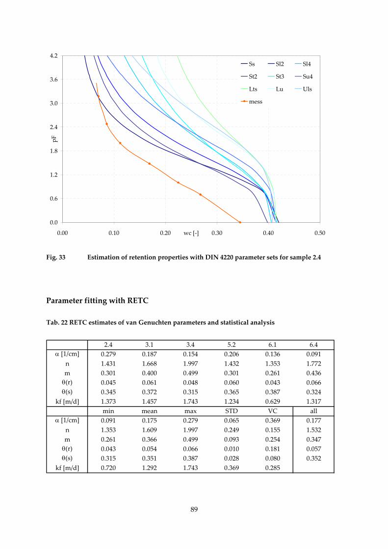
0.0
0.6
1.2
1.8
2.4
3.0
3.6
4.2
0.00 0.10 0.20 0.30 0.40 0.50wc [‐]
pF
Ss Sl2 Sl4
St2 St3 Su4
Lts Lu Uls
mess
Fig. 33 Estimation of retention properties with DIN 4220 parameter sets for sample 2.4
Parameter fitting with RETC
Tab. 22 RETC estimates of van Genuchten parameters and statistical analysis
2.4 3.1 3.4 5.2 6.1 6.4α [1/cm] 0.279 0.187 0.154 0.206 0.136 0.091
n 1.431 1.668 1.997 1.432 1.353 1.772m 0.301 0.400 0.499 0.301 0.261 0.436
θ(r) 0.045 0.061 0.048 0.060 0.043 0.066θ(s) 0.345 0.372 0.315 0.365 0.387 0.324
kf [m/d] 1.373 1.457 1.743 1.234 0.629 1.317min mean max STD VC all
α [1/cm] 0.091 0.175 0.279 0.065 0.369 0.177n 1.353 1.609 1.997 0.249 0.155 1.532m 0.261 0.366 0.499 0.093 0.254 0.347
θ(r) 0.043 0.054 0.066 0.010 0.181 0.057θ(s) 0.315 0.351 0.387 0.028 0.080 0.352
kf [m/d] 0.720 1.292 1.743 0.369 0.285
89

90
Van Genuchten parameters were fitted to the determined retention curves. In contrast to the
methods above, not correlated information is applied to estimate the unknown retention
characteristics but measured van Genuchten parameters are optimized to reproduce the
measured water content – water tension relation.
Tab. 22 concludes the results of the parameter fitting with RETC. Conductivity values are
given as estimated by ROSETTA from the RETC‐fitted van Genuchten parameters. The
upper part gives the van Genuchten values and saturated conductivity for every soil sample,
the lower part gives a statistical evaluation of the findings. The single values correspond
roughly to sands (scaling parameter, residual water content) or loamy sand (increase
parameter, saturated conductivity). Saturated water contents are slightly lower than
literature values, probably a consequence of the determination for disturbed samples. The
statistical analysis shows that the heterogeneity of the different parameters varies
considerably. The variation coefficient is biggest for the scaling parameter and smallest for
the saturated conductivity. The mean values correspond satisfyingly with the “all” values
that were obtained by fitting the parameters to all samples at the same time. Fitting quality
was generally high, rRMSE was less than 2 % for all samples, less than 5 % for the all
parameter set. The fitting quality is visualized in Fig. 34. Generally the curves are well fitted.
There is no systematic tendency detectable, that higher or lower suction heads are
reproduced worse. The curves of generally higher or water content at same pressure head
also do not give worse approximations. Irregularities in the measured curve are not
reproduced by the program, e. g. the step of curve LL 6.1 is not found in the fitted course.
This is mainly because of the limited flexibility of van Genuchten model.
A trail to reduce the number of estimation points was carried out. With four points it was
still possible to reproduce the retention curve satisfyingly (rRMSE < 10 %). The fitting was
generally better if the input values covered a broad range of water tensions.
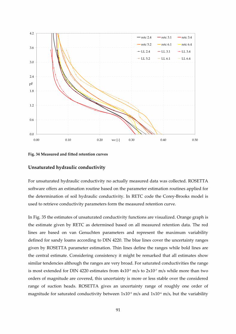
0.0
0.6
1.2
1.8
2.4
3.0
3.6
4.2
0.00 0.10 0.20 0.30 0.40 0.50wc [‐]
pF
retc 2.4 retc 3.1 retc 3.4
retc 5.2 retc 6.1 retc 6.4
LL 2.4 LL 3.1 LL 3.4
LL 5.2 LL 6.1 LL 6.4
Fig. 34 Measured and fitted retention curves
Unsaturated hydraulic conductivity
For unsaturated hydraulic conductivity no actually measured data was collected. ROSETTA
software offers an estimation routine based on the parameter estimation routines applied for
the determination of soil hydraulic conductivity. In RETC code the Corey‐Brooks model is
used to retrieve conductivity parameters form the measured retention curve.
In Fig. 35 the estimates of unsaturated conductivity functions are visualized. Orange graph is
the estimate given by RETC as determined based on all measured retention data. The red
lines are based on van Genuchten parameters and represent the maximum variability
defined for sandy loams according to DIN 4220. The blue lines cover the uncertainty ranges
given by ROSETTA parameter estimation. Thin lines define the ranges while bold lines are
the central estimate. Considering consistency it might be remarked that all estimates show
similar tendencies although the ranges are very broad. For saturated conductivities the range
is most extended for DIN 4220 estimates from 4x10‐5 m/s to 2x10‐7 m/s while more than two
orders of magnitude are covered, this uncertainty is more or less stable over the considered
range of suction heads. ROSETTA gives an uncertainty range of roughly one order of
magnitude for saturated conductivity between 1x10‐5 m/s and 1x10‐6 m/s, but the variability
91
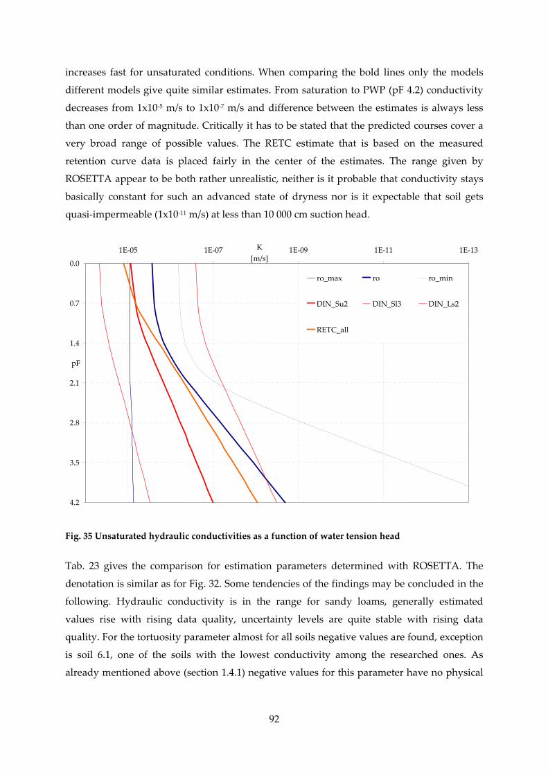
increases fast for unsaturated conditions. When comparing the bold lines only the models
different models give quite similar estimates. From saturation to PWP (pF 4.2) conductivity
decreases from 1x10‐5 m/s to 1x10‐7 m/s and difference between the estimates is always less
than one order of magnitude. Critically it has to be stated that the predicted courses cover a
very broad range of possible values. The RETC estimate that is based on the measured
retention curve data is placed fairly in the center of the estimates. The range given by
ROSETTA appear to be both rather unrealistic, neither is it probable that conductivity stays
basically constant for such an advanced state of dryness nor is it expectable that soil gets
quasi‐impermeable (1x10‐11 m/s) at less than 10 000 cm suction head.
0.0
0.7
1.4
2.1
2.8
3.5
4.2
1E‐131E‐111E‐091E‐071E‐05 K [m/s]
pF
ro_max ro ro_min
DIN_Su2 DIN_Sl3 DIN_Ls2
RETC_all
Fig. 35 Unsaturated hydraulic conductivities as a function of water tension head
Tab. 23 gives the comparison for estimation parameters determined with ROSETTA. The
denotation is similar as for Fig. 32. Some tendencies of the findings may be concluded in the
following. Hydraulic conductivity is in the range for sandy loams, generally estimated
values rise with rising data quality, uncertainty levels are quite stable with rising data
quality. For the tortuosity parameter almost for all soils negative values are found, exception
is soil 6.1, one of the soils with the lowest conductivity among the researched ones. As
already mentioned above (section 1.4.1) negative values for this parameter have no physical
92
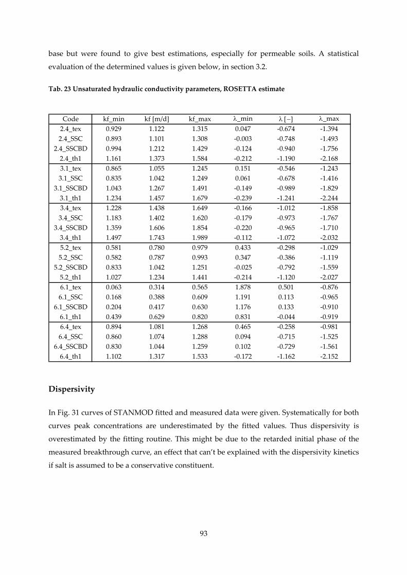
base but were found to give best estimations, especially for permeable soils. A statistical
evaluation of the determined values is given below, in section 3.2.
Tab. 23 Unsaturated hydraulic conductivity parameters, ROSETTA estimate
Code kf_min kf [m/d] kf_max λ_min λ [−] λ_max2.4_tex 0.929 1.122 1.315 0.047 ‐0.674 ‐1.3942.4_SSC 0.893 1.101 1.308 ‐0.003 ‐0.748 ‐1.493
2.4_SSCBD 0.994 1.212 1.429 ‐0.124 ‐0.940 ‐1.7562.4_th1 1.161 1.373 1.584 ‐0.212 ‐1.190 ‐2.1683.1_tex 0.865 1.055 1.245 0.151 ‐0.546 ‐1.2433.1_SSC 0.835 1.042 1.249 0.061 ‐0.678 ‐1.416
3.1_SSCBD 1.043 1.267 1.491 ‐0.149 ‐0.989 ‐1.8293.1_th1 1.234 1.457 1.679 ‐0.239 ‐1.241 ‐2.2443.4_tex 1.228 1.438 1.649 ‐0.166 ‐1.012 ‐1.8583.4_SSC 1.183 1.402 1.620 ‐0.179 ‐0.973 ‐1.767
3.4_SSCBD 1.359 1.606 1.854 ‐0.220 ‐0.965 ‐1.7103.4_th1 1.497 1.743 1.989 ‐0.112 ‐1.072 ‐2.0325.2_tex 0.581 0.780 0.979 0.433 ‐0.298 ‐1.0295.2_SSC 0.582 0.787 0.993 0.347 ‐0.386 ‐1.119
5.2_SSCBD 0.833 1.042 1.251 ‐0.025 ‐0.792 ‐1.5595.2_th1 1.027 1.234 1.441 ‐0.214 ‐1.120 ‐2.0276.1_tex 0.063 0.314 0.565 1.878 0.501 ‐0.8766.1_SSC 0.168 0.388 0.609 1.191 0.113 ‐0.965
6.1_SSCBD 0.204 0.417 0.630 1.176 0.133 ‐0.9106.1_th1 0.439 0.629 0.820 0.831 ‐0.044 ‐0.9196.4_tex 0.894 1.081 1.268 0.465 ‐0.258 ‐0.9816.4_SSC 0.860 1.074 1.288 0.094 ‐0.715 ‐1.525
6.4_SSCBD 0.830 1.044 1.259 0.102 ‐0.729 ‐1.5616.4_th1 1.102 1.317 1.533 ‐0.172 ‐1.162 ‐2.152
Dispersivity
In Fig. 31 curves of STANMOD fitted and measured data were given. Systematically for both
curves peak concentrations are underestimated by the fitted values. Thus dispersivity is
overestimated by the fitting routine. This might be due to the retarded initial phase of the
measured breakthrough curve, an effect that can’t be explained with the dispersivity kinetics
if salt is assumed to be a conservative constituent.
93
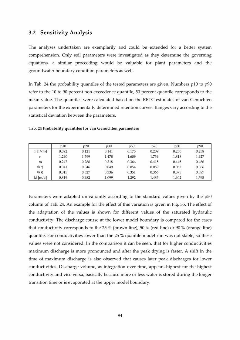
3.2 Sensitivity Analysis
The analyses undertaken are exemplarily and could be extended for a better system
comprehension. Only soil parameters were investigated as they determine the governing
equations, a similar proceeding would be valuable for plant parameters and the
groundwater boundary condition parameters as well.
In Tab. 24 the probability quantiles of the tested parameters are given. Numbers p10 to p90
refer to the 10 to 90 percent non‐exceedence quantile, 50 percent quantile corresponds to the
mean value. The quantiles were calculated based on the RETC estimates of van Genuchten
parameters for the experimentally determined retention curves. Ranges vary according to the
statistical deviation between the parameters.
Tab. 24 Probability quantiles for van Genuchten parameters
p10 p20 p30 p50 p70 p80 p90α [1/cm] 0.092 0.121 0.141 0.175 0.209 0.230 0.258
n 1.290 1.399 1.478 1.609 1.739 1.818 1.927m 0.247 0.288 0.318 0.366 0.415 0.445 0.486
θ(r) 0.041 0.046 0.049 0.054 0.059 0.062 0.066θ(s) 0.315 0.327 0.336 0.351 0.366 0.375 0.387
kf [m/d] 0.819 0.982 1.099 1.292 1.485 1.602 1.765
Parameters were adapted univariantly according to the standard values given by the p50
column of Tab. 24. An example for the effect of this variation is given in Fig. 35. The effect of
the adaptation of the values is shown for different values of the saturated hydraulic
conductivity. The discharge course at the lower model boundary is compared for the cases
that conductivity corresponds to the 25 % (brown line), 50 % (red line) or 90 % (orange line)
quantile. For conductivities lower than the 25 % quantile model run was not stable, so these
values were not considered. In the comparison it can be seen, that for higher conductivities
maximum discharge is more pronounced and after the peak drying is faster. A shift in the
time of maximum discharge is also observed that causes later peak discharges for lower
conductivities. Discharge volume, as integration over time, appears highest for the highest
conductivity and vice versa, basically because more or less water is stored during the longer
transition time or is evaporated at the upper model boundary.
94

‐3.5
‐2.8
‐2.1
‐1.4
‐0.7
0.0
0 5 10 15 20 25 30 35t [d]
Q [mm/d]
k_0.25 standard k_0.9
Fig. 36 Discharge courses for different hydraulic conductivities
Fig. 37 displays the relative change of water content six days after irrigation in relation to the
water content of the “standard” case. Lines that are shorter than the 0.1 – 0.9 range did not
perform stable beyond the displayed range and were thus not considered completely. The
courses of transformation parameter, hydraulic conductivity and residual water content
conduct a fairly linear. For example with increasing m the water content decreases after six
days proportionally. The increase parameter has a negative sensitivity from 0.3 – 0.5 quantile
and becomes insensitive for further increase. Saturated water content and scaling parameter
are both not monotonous. While for the scaling parameter minimum point is at the 0.5
quantile, saturated water content decreases for quantiles smaller than 0.3 and than increases
to 0.7 non‐exceedence probability.
Similar sensitivity courses are found for maximum discharge and accumulated discharge
although parameters may show different courses. The findings confirm that the processes of
water transport and storage in the unsaturated soil zone are highly non‐linear and great care
has to be spent on parameter definition and calibration.
95

‐30
‐20
‐10
0
10
20
30
40
0 0.1 0.2 0.3 0.4 0.5 0.6 0.7 0.8 0.9 1
param. prob.
rel.
Δwc [%
]
a n m k tr ts
Fig. 37 Sensitivities of water content to van‐Genuchten parameters
In Tab. 25 the sensitivity indexes of the parameters that showed linear behaviour are
concluded. Parameter – target variable combinations with non‐linear behaviour are labelled
“nl”. It is apparent that for the different target values parameters conduct different. The by
far highest sensitivity is found for maximum discharge and hydraulic conductivity. Other
important relations exist between water content and transformation parameter as well as
maximum discharge and residual water content. The generally lower sensitivities of
accumulated discharge might be explained with the integrative character of this parameter,
after a certain amount of time all water that goes in goes out again and differences in the
course are compensated by the accumulation.
Tab. 25 Sensitivity indexes for the different soil parameters and target variables
96
SI(Q_acc) SI(Qmax) SI(wc)α ‐0.203 ‐0.334 nln ‐0.077 ‐0.125 nlm nl 0.244 ‐0.451k nl 1.803 ‐0.306θr 0.023 0.405 0.280θs nl nl nl

3.3 Calibration and Validation
Calibration was carried out for ’93 – ’94 irrigation season with seven days irrigation
frequency. Validation was conducted with 14 and 21 days irrigation frequency as well as
with ’91 – ’92 and ’92 – ’93 irrigation seasons each with seven day frequency. The aim was to
determine if climate driving forces or flow boundaries have a bigger influence on model
performance.
Relative water content was used as target variable for the calibration. When left to the choice
it is disadvantageous compared to flow information because it is only an indirect measure of
water movement. Percolation at the lower model boundary is difficult to determine,
especially where no drainage is installed. In comparison soil water content monitoring is
easily set up. Another advantage is the higher resolution with that it can be determined. Both
factors make soil water content an interesting target variable for the description of soil water
movement.
SiWaPro also includes a parameter optimization algorithm for inverse estimation of soil
hydraulic parameters from measured transient or steady‐state flow. The inverse estimation
was not tested successfully probably because boundary conditions were too dynamic
respectively the repeated water application did not permit to identify an optimum parameter
configuration.
3.3.1 Calibration parameters and model performance
Tab. 26 Parameters addressed during the calibration
initial value final valueα [1/m] 17.7 14.3
n 1.53 1.61m 0.347 0.347
k [m/d] 1.29 2.13λ ‐1.92 ‐1.32*Aqh ‐0.169 ‐0.113
Bqh ‐0.027 ‐0.081θr 0.057 0.057θs 0.352 0.398
*tortuosity parameter had to be adapted afterwards again in order to enhance model stability
97
98
Calibration was focused on soil and groundwater boundary condition parameters. The initial
estimates and final values are concluded in Tab. 26. Initial values were basically obtained
from the parameter configuration determined by RETC under consideration of all
determined retention data values. Biggest adaptations had to be undertaken on saturated
conductivity, tortuosity parameter and saturated water content. Transformation parameter
and residual water content could be left unchanged.
Visual fitting quality
Relative water content in the four diagnostic layers was the target variable for the calibration.
The values were collected by defined observation points at the specific coordinates. A
visualization of the comparison between some calibration alternatives is given in Fig. 38.
Varied parameter is the scaling factor Bqh of the [Hopmans, 1989] groundwater approach.
The upper diagraph shows the modeled development of water content dynamics over the
irrigation period. All alternatives perform fairly well with regard to the reproduction of
measured values. _b0.08 and _b0.06 alternatives have the constraint, that not all irrigation
cycles are reproduced. The image suggests that the measurement of field capacity after 48
hours was too late, soil was already in the drying phase at this point of time and maximum
moisture contents are not covered by the measurements. The differences in the performance
of the alternatives are more pronounced at 120 cm depth (lower diagraph). Alternatives
_b0.08 and _b0.04 overestimate the average water content, which is expressed by a high bias
for these alternatives. Amplitude of the water content course is overestimated by _b0.08 and
reproduced sufficiently for alternatives _b0.06 and _b0.04. Deviation for single values is
better for _0.04 while overall performance accounts for _0.06.
Generally it must be stated that soil and groundwater parameters where more sensitive in
the lower soil layers, probably because the predominant influence of climate drivers over the
water movement drivers diminishes. As a consequence, if a choice is necessary and possible,
it would be preferable to measure water content dynamics in a more profound soil layer in
order to be more certain about determining processes.
Besides from the quantitative and objective performance quality parameters (evaluation
below), the visualization of water content development is valuable because determinant
effects are identified more easily. E.g. in Fig. 38 at 120 cm depth the PPs for alternatives
_b0.06 and _b0.04 were similar but the visualization reveals that drying phase is reproduced
to slow so that the movement in the course can’t be explained.

0
5
10
15
20
25
30
35
01.11.93 21.11.93 11.12.93 31.12.93 20.01.94 09.02.94 01.03.94 21.03.94
wc [%]
mess k2.1_a0.176_b0.08 k2.1_a0.176_b0.06 p2.1_a0.176_b0.04
0
5
10
15
20
25
30
35
01.11.93 21.11.93 11.12.93 31.12.93 20.01.94 09.02.94 01.03.94 21.03.94
wc [%]
mess k2.1_a0.176_b0.08 k2.1_a0.176_b0.06 k2.1_a0.176_b0.04
Fig. 38 Calibration performance for water contents at 15 cm and 120 cm depth
For some events the general assumption of 130 mm irrigation depth proved inconvenient
and does probably not correspond to reality. E. g. the pronounced period of lower humidity
values as well for “before irrigation” as for “after irrigation” events indicates that during that
99

time not the same amount of water reached the lower soil zone. No calibration configuration
allowed representing as well this period of low values as the regular regime during the rest
of the irrigation season. This drawback underlines that it is important to capture the water
balance in order to explain model ‐ or measured value irregularities.
Performance quality parameters
A part of the determination of performance evaluation was conducted automatized, an
example is given in Fig. 39. A MATLAB script provided by F. Blumensaat was adapted to the
specific situation. Similar to Fig. 38 the upper plot shows the courses of measured and
simulated data. For every calibration run bias, NSE and IoA were determined. Lower plot
shows accumulated values taken for the measurement dates. Increase coefficients are
specified for both accumulation curves and deviation determined as ratio of simulated to
measured increase coefficient. The plot of accumulated values determined in order to
identify possible changes in the regime or systematic errors that are not detected by the bias.
03/11/1993 01/12/1993 29/12/1993 27/01/1994 24/02/1994 25/03/19940
10
20
30
40
rh [%
]
Bias =2.031NSE =0.544IoA =0.683
ref datasim data
03/11/1993 01/12/1993 29/12/1993 27/01/1994 24/02/1994 25/03/19940
0.5
1
1.5
2
x 108
cum rh [%
]
est =1.99e+008ref =2.15e+008dev =0.927
ref datasim data
Fig. 39 Quality assessment of a calibration version
100

Tab. 27 Fitting quality parameters of calibration and validation
93 ‐ ʹ94 7d 0 ‐ 30 cm 30 ‐ 60 cm 60 ‐ 90 cm 90 ‐ 120 cm meanbias 0.026 0.032 0.029 0.047 0.034RMSE 0.031 0.039 0.042 0.065 0.044rRMSE 0.065 0.082 0.088 0.137 0.093NSE 0.79 0.65 0.68 0.55 0.67IoA 0.81 0.77 0.69 0.64 0.73R² 0.87 0.83 0.69 0.61 0.75
93 ‐ ʹ94 14d 0 ‐ 30 cm 30 ‐ 60 cm 60 ‐ 90 cm 90 ‐ 120 cm meanbias 0.054 0.058 0.062 0.047 0.063RMSE 0.063 0.071 0.084 0.107 0.081rRMSE 0.132 0.149 0.177 0.225 0.171NSE 0.74 0.69 0.65 0.53 0.66IoA 0.78 0.73 0.66 0.61 0.70R² 0.77 0.74 0.62 0.59 0.68
93 ‐ ʹ94 21d 0 ‐ 30 cm 30 ‐ 60 cm 60 ‐ 90 cm 90 ‐ 120 cm meanbias 0.060 0.067 0.083 0.075 0.071RMSE 0.068 0.089 0.093 0.097 0.087rRMSE 0.142 0.186 0.195 0.204 0.182NSE 0.66 0.61 0.58 0.51 0.67IoA 0.74 0.72 0.66 0.61 0.68R² 0.68 0.65 0.53 0.57 0.61
91 ‐ ʹ92 7d 0 ‐ 30 cm 30 ‐ 60 cm 60 ‐ 90 cm 90 ‐ 120 cm meanbias 0.023 0.040 0.017 0.050 0.030RMSE 0.037 0.037 0.050 0.065 0.045rRMSE 0.079 0.078 0.106 0.146 0.102NSE 0.83 0.66 0.69 0.55 0.68IoA 0.81 0.79 0.74 0.67 0.75R² 0.83 0.79 0.64 0.59 0.71
92 ‐ ʹ93 7d 0 ‐ 30 cm 30 ‐ 60 cm 60 ‐ 90 cm 90 ‐ 120 cm meanbias 0.036 0.043 0.040 0.052 0.042RMSE 0.050 0.047 0.057 0.080 0.076rRMSE 0.105 0.098 0.120 0.106 0.107NSE 0.79 0.67 0.70 0.58 0.68IoA 0.85 0.78 0.73 0.66 0.75R² 0.79 0.77 0.67 0.58 0.70
mean 0 ‐ 30 cm 30 ‐ 60 cm 60 ‐ 90 cm 90 ‐ 120 cm meanbias 0.040 0.048 0.046 0.054RMSE 0.050 0.056 0.065 0.083rRMSE 0.104 0.119 0.137 0.164NSE 0.76 0.66 0.66 0.54IoA 0.80 0.76 0.70 0.64R² 0.79 0.76 0.63 0.59
101
102
Tab. 27 concludes the results of the calibration and validation process. The considerations
given for the visual evaluation are confirmed by the PPs. Lower soil layers are generally
represented worse by the calibrated as well as the validated model. If the model quality was
enhanced for the lower layers it was on the cost of an over‐proportionally stronger
deterioration of fitting quality in the upper layers. As a reason the effect previously
mentioned might be stated. For arid climates evaporation is the predominant driver for
water movement in the upper layer while further down percolation increases in importance.
Both processes have to be represented sufficiently.
For the validation four configurations were considered, two with different irrigation regime
(’93 – ’94 14d and 21d) and two with different climatic boundaries (’91 – ’92 7d and ’92 – ’93
7d). It is apparent that validation quality for different irrigation regime was globally worse
than for different climatic boundaries. All performance indicators range lower for the
irrigation cases than for the climate cases. In comparison between the two irrigation cases the
one that is “further away” from the calibration case performs worse. Hence model
performance is less sensitive towards climatic boundaries than towards anthropogenic water
regime. It should be thus intended that the probable range of water donations is considered
during the calibration phase. Nevertheless, even for the 21 day validation period
performance quality is satisfying.
Each performance quality parameter has advantages and disadvantages. Only the proper
combination of different parameters permits an integral evaluation of model performance.
The choice which parameters should be applied depends on modelling purpose and the type
of target variable that is considered.
Bias allows detecting systematic errors; it is especially relevant for water balance
considerations. A drawback is that systematic errors of deviation compensate each other. E.
g. if highest and lowest water contents are over‐ respectively underestimated by the same
extend no bias is predicted. In the application bias performs generally well, it is for all cases
less than ten percent of mean humidity values. Highest bias values are found for 21 d
irrigation case and for the two deeper soil layers. Still differences are not very pronounced.
RMSE is avoiding the deviation insensitivity of bias and buffers the influence of outliers is
buffered. RMSE values are globally slightly higher than bias. This advocates a certain
influence of systematic deviation misestimation although the effect can’t be to strong, as
mean difference is less than 20 % between the values. With regards to performance

103
tendencies again in greater depths and with minor irrigation frequency estimation quality is
worse. But for RMSE depth is a stronger influence on deterioration.
The parameter rRMSE expresses the ratio between RMSE and mean rh, tendencies are thus
the same as for RMSE but differences are more pronounced.
NSE is an illustrative parameter as it delivers two prominent points of reference for NSE = 0
model performance is worse than mean value. For NSE = 1 the model matches perfectly
measured values. For the calibration and validation NSEs are generally higher than 0.5 with
lowest values for the deepest soil layer. The mean performance of the irrigation frequency
validation cases is only slightly worse than for the calibration. For climate boundary
validation it is even slightly better. A clear tendency is found for soil depth, model
performance gets worse in the lower soil layers. This indicates that the course of water
content is reproduced for the validation with a high confidence but within the distinct cases
performance quality is heterogeneous.
The capability of IoA to consider relative differences between comparison pairs (see section
2.5) proved valuable in order to estimate lower “before irrigation” values as well as higher
“after irrigation” values. For the IoA variability again is more driven by depth than by
configuration. Lowest IoAs are found in the deepest soil layer, indicating that there the
dynamic of either low or high soil moisture values is reproduced worse than in average. IoA
is especially valuable in combination with the visual assessment as it supports to focus on
certain performance aspects.
R²s describe the proportion of the variance of measured data in the variance of the estimation
function. As NSE it is a parameter that supports the evaluation of the modeling course. The
R² values found partly affirm the findings of NSE. Variability is bigger for soil depths than
for validation cases. Nevertheless heterogeneity between the validation cases is bigger than
for NSE.
Model performance assessment with respect to both spatial distribution of the performance
and model configuration proved to be an efficient tool for the identification of systematic
weaknesses and gives a quantifiable background for model enhancement and vulnerability
for model application.

Integrated performance quality
Performance utility was calculated for the calibration and validation cases. The motivation
was rather to introduce the method and test applicability as no convenient method was
found. In Tab. 28 the thresholds of the utility function and weighting coefficients for the PPs
are concluded. Assumptions are somewhat conceptual but serve to demonstrate the
performance of the method.
Tab. 28 utility function thresholds and weighting coefficients for performance utility analysis
93 ‐ ʹ94 7d min. threshold max. threshold weightbias 0.1 0 0.2RMSE 0.2 0 0.2rRMSE ‐ ‐ ‐NSE 0 1 0.2IoA 0 1 0.2R² 0 1 0.2
Utility functions are assumed to be linear between the thresholds defined. For values not
more than minimum threshold utility value is assumed to be zero, for values not less than
maximum threshold they equal one. For bias and RMSE minimum thresholds were defined
according to calibration cases that performed “bad”. rRMSE was not considered as it is
directly dependent form RMSE. The thresholds for NSE, IoA and R² are defined by
characteristic values of these parameters. Weighting coefficients were distributed equal
between the PPs as no special modeling aspect was favored specifically.
A comparison of performance utilities is given in Fig. 40. Denotation refers to the cases
discussed above; “optium” represents a virtual perfect model. As to be seen calibration and
validation with ’91 – ’92 climate reach highest performance qualities. Both climate validation
score better than the irrigation validations. Bias was in average the hardest performance
criterion with lowest partial utility values. IoA generally contributes the biggest portion.
104

0.0
0.2
0.4
0.6
0.8
1.0
optimum 93 ‐ ʹ94 7d 93 ‐ ʹ94 14d 93 ‐ ʹ94 21d 91 ‐ ʹ92 7d 92 ‐ ʹ93 7d
bias RMSE NSE IoA R²
Fig. 40 Performance utilities for an virtual optimum model, calibration and validation cases
3.4 Modeling results
In the following some findings on model performance and evaluation methods are
concluded. The section is somewhat brief because the evaluation of scenarios below refers to
some aspects similarly.
3.4.1 Numerical stability and mass balance
Mass balance problems were inherent for the model runs that could not be solved neither by
refinement of the temporal or spatial resolution nor by increase of expense in the simulation
control. The sharp changes between extreme dry climate out of irrigation season and the
highly dynamic water fluxes during irrigation caused mass imbalances for the first few
irrigation cycles but over all mass balance error, calculated as difference between inflow and
outflow was controlled to not to exceeded five percent.
Some parameter combinations proved to cause numerical instabilities that caused oscillating
solutions and / or a breaking off of the simulation. Although it is hard to define a physical
base for these phenomena they shall be mentioned in order to allow further research. Under
extremely dry conditions, when small amounts of water faced big potential gradients mass
105
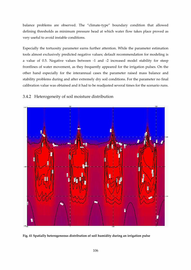
balance problems are observed. The “climate‐type” boundary condition that allowed
defining thresholds as minimum pressure head at which water flow takes place proved as
very useful to avoid instable conditions.
Especially the tortuosity parameter earns further attention. While the parameter estimation
tools almost exclusively predicted negative values; default recommendation for modeling is
a value of 0.5. Negative values between ‐1 and ‐2 increased model stability for steep
frontlines of water movement, as they frequently appeared for the irrigation pulses. On the
other hand especially for the interannual cases the parameter raised mass balance and
stability problems during and after extremely dry soil conditions. For the parameter no final
calibration value was obtained and it had to be readjusted several times for the scenario runs.
3.4.2 Heterogeneity of soil moisture distribution
Fig. 41 Spatially heterogeneous distribution of soil humidity during an irrigation pulse
106
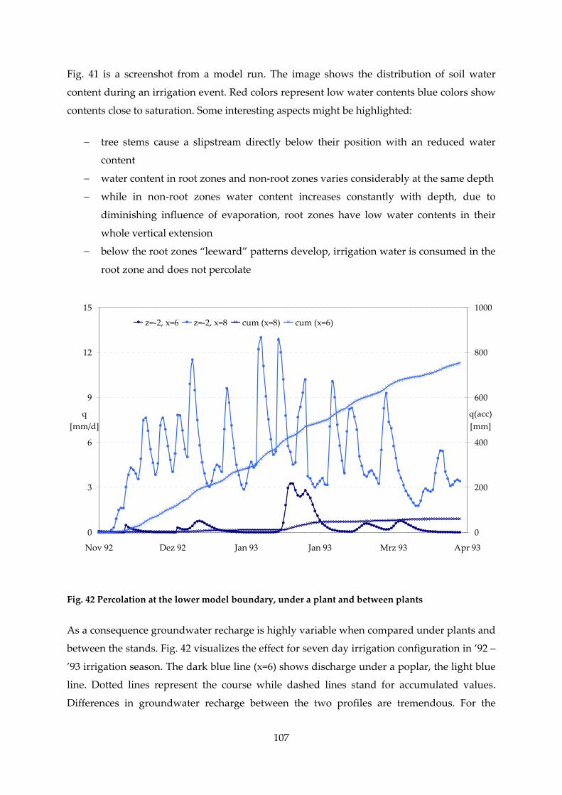
Fig. 41 is a screenshot from a model run. The image shows the distribution of soil water
content during an irrigation event. Red colors represent low water contents blue colors show
contents close to saturation. Some interesting aspects might be highlighted:
− tree stems cause a slipstream directly below their position with an reduced water
content
− water content in root zones and non‐root zones varies considerably at the same depth
− while in non‐root zones water content increases constantly with depth, due to
diminishing influence of evaporation, root zones have low water contents in their
whole vertical extension
− below the root zones “leeward” patterns develop, irrigation water is consumed in the
root zone and does not percolate
0
3
6
9
12
15
Nov 92 Dez 92 Jan 93 Jan 93 Mrz 93 Apr 93
q [mm/d]
0
200
400
600
800
1000
q(acc) [mm]
z=‐2, x=6 z=‐2, x=8 cum (x=8) cum (x=6)
Fig. 42 Percolation at the lower model boundary, under a plant and between plants
As a consequence groundwater recharge is highly variable when compared under plants and
between the stands. Fig. 42 visualizes the effect for seven day irrigation configuration in ’92 –
’93 irrigation season. The dark blue line (x=6) shows discharge under a poplar, the light blue
line. Dotted lines represent the course while dashed lines stand for accumulated values.
Differences in groundwater recharge between the two profiles are tremendous. For the
107
108
between plants profile almost every irrigation donation causes deep percolation for some
donations (the two maximum peaks in January) it accumulates to 65 mm or half of the total
irrigation depth. The total amount accumulates to 754 mm of percolating water or 29 % of the
total irrigation depth. In contrast below the plant stand deep percolation occurs only
occasionally. Only one “mayor” event in January with 40 mm over two irrigation cycles
accounts for more than half of the total percolation. Only 70 mm or 3 % of the total seasonal
irrigation volume are lost by deep percolation. If the balance is drawn for the total irrigation
parcel, where only 8.3 % of the soil is occupied by deep root zones4, under this assumption
effective percolation is 711 mm.
3.4.3 Groundwater recharge and salt balance
Tab. 29 concludes the results of the water balance as drawn above, irrigation and
precipitation are either evaporated / transpired or percolated, the portions of storage change
in the soil and incorporation by plants are neglected as inferior compared to the other
balance components. It is apparent that percolation portion is more than proportionally
increased with higher irrigations frequencies. While percolation coefficient (as ratio of
percolation to irrigation plus precipitation) is 0.27 for the seven day irrigation case it
diminishes to 0.17 for the 21 day case, values are given as c_per in Tab. 29. The coefficients
are rather stable for the different seasons although precipitation depths vary considerably
between 320 mm in ’92 – ’93 and 45 mm in ’93 – ’94.
The salt balance considerations are based on the simplified concentration – leaching ‐ model
proposed by [Ayers, 1985]. He defines a concentration factor as dependent variable of
percolation coefficient and assumes that in average soil salinity increases multiplied by
concentration factor and irrigation water salinity. Ayers proposes the model for calculation
with ECs but as conductivity is directly dependent from concentration (see section 2.3.3), the
model is adapted to a load‐based balance. Assumptions are that initial salt concentration in
soil and irrigation water are equally at 0.49 g/l (1.5 dS/m). Precipitation water is considered
as salt free. Complete mixture of irrigation water and residual soil water is guaranteed at
every time. The balance components given in Tab. 29 are determined as following (F. 36):
4 16 squares of 1 m x 1 m out of an parcel of 12 m x 16 m

ETcIIper
resIper
q*)c1(q*cllll
−−=
−= F. 36
with: lper percolation load [M/L²]
lI irrigation water load [M/L²]
lres residual load [M/L²]
cI irrigation water concentration [M/L³]
qI depth of irrigation [L³/L²]
cc concentration coefficient [‐]
qET depth of evapotranspiration [L³/L²]
The results of the mass transport balance given by F. 36 are concluded in Tab. 29. Water
balance indicates that the water is applied inefficiently at higher irrigation depths. Parameter
c_per expresses the ratio of applied water to percolated water with 0.27 the values for seven
day irrigation is almost 40 % higher than for 21 day configuration. But also ET is reduced
which confirms the finding of [Riu, 2004] that trees with more frequent irrigation grow
stronger. Restrictively it has to be mentioned that evaporation and transpiration can’t be
evaluated separately. Climate seems to have a minor role on groundwater recharge from
irrigation excess. The c_per values hardly change for the different years, as a slight tendency
the c_per for seven day irrigation increases with higher precipitation rates.
For all cases a mayor portion of the salt is transferred to the lower soil zone and contributes
sooner or later to groundwater salinization. As salt load is proportional to irrigation depth
(biased by precipitation), seven day alternative shows highest salt input rates (NaCl_in). For
the residual content the tendency is reverted. As to be expected with higher irrigation excess
leaching portion is bigger and less salt accumulates in the soil zone. The difference between
percolated salt load is much more pronounced than for residual loads. While percolated load
in average of seven day irrigation is four times higher than for 21 day irrigation, the residual
content is about 1.5 times higher for 21 day irrigation than for seven day regime.
109
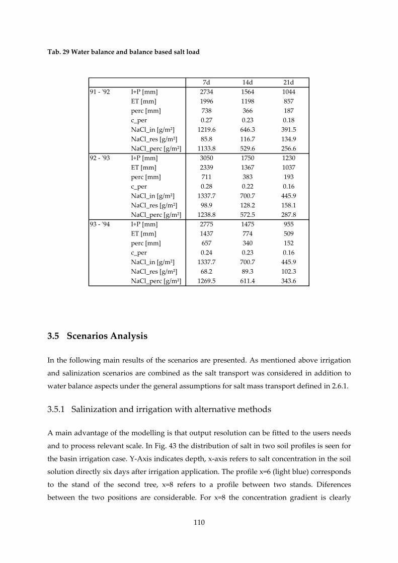
Tab. 29 Water balance and balance based salt load
7d 14d 21d91 ‐ ʹ92 I+P [mm] 2734 1564 1044
ET [mm] 1996 1198 857perc [mm] 738 366 187c_per 0.27 0.23 0.18NaCl_in [g/m²] 1219.6 646.3 391.5NaCl_res [g/m²] 85.8 116.7 134.9NaCl_perc [g/m²] 1133.8 529.6 256.6
92 ‐ ʹ93 I+P [mm] 3050 1750 1230ET [mm] 2339 1367 1037perc [mm] 711 383 193c_per 0.28 0.22 0.16NaCl_in [g/m²] 1337.7 700.7 445.9NaCl_res [g/m²] 98.9 128.2 158.1NaCl_perc [g/m²] 1238.8 572.5 287.8
93 ‐ ʹ94 I+P [mm] 2775 1475 955ET [mm] 1437 774 509perc [mm] 657 340 152c_per 0.24 0.23 0.16NaCl_in [g/m²] 1337.7 700.7 445.9NaCl_res [g/m²] 68.2 89.3 102.3NaCl_perc [g/m²] 1269.5 611.4 343.6
3.5 Scenarios Analysis
In the following main results of the scenarios are presented. As mentioned above irrigation
and salinization scenarios are combined as the salt transport was considered in addition to
water balance aspects under the general assumptions for salt mass transport defined in 2.6.1.
3.5.1 Salinization and irrigation with alternative methods
A main advantage of the modelling is that output resolution can be fitted to the users needs
and to process relevant scale. In Fig. 43 the distribution of salt in two soil profiles is seen for
the basin irrigation case. Y‐Axis indicates depth, x‐axis refers to salt concentration in the soil
solution directly six days after irrigation application. The profile x=6 (light blue) corresponds
to the stand of the second tree, x=8 refers to a profile between two stands. Diferences
between the two positions are considerable. For x=8 the concentration gradient is clearly
110
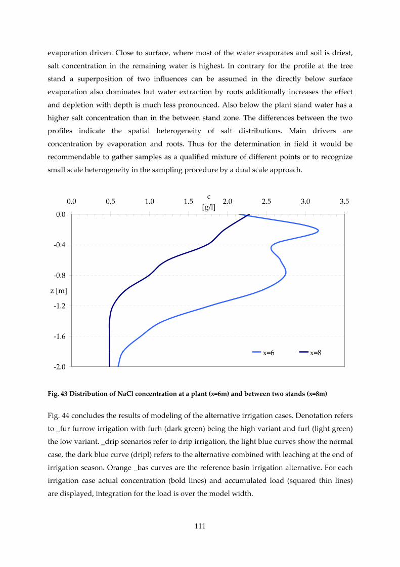
evaporation driven. Close to surface, where most of the water evaporates and soil is driest,
salt concentration in the remaining water is highest. In contrary for the profile at the tree
stand a superposition of two influences can be assumed in the directly below surface
evaporation also dominates but water extraction by roots additionally increases the effect
and depletion with depth is much less pronounced. Also below the plant stand water has a
higher salt concentration than in the between stand zone. The differences between the two
profiles indicate the spatial heterogeneity of salt distributions. Main drivers are
concentration by evaporation and roots. Thus for the determination in field it would be
recommendable to gather samples as a qualified mixture of different points or to recognize
small scale heterogeneity in the sampling procedure by a dual scale approach.
‐2.0
‐1.6
‐1.2
‐0.8
‐0.4
0.0
0.0 0.5 1.0 1.5 2.0 2.5 3.0 3.5c
[g/l]
z [m]
x=6 x=8
Fig. 43 Distribution of NaCl concentration at a plant (x=6m) and between two stands (x=8m)
Fig. 44 concludes the results of modeling of the alternative irrigation cases. Denotation refers
to _fur furrow irrigation with furh (dark green) being the high variant and furl (light green)
the low variant. _drip scenarios refer to drip irrigation, the light blue curves show the normal
case, the dark blue curve (dripl) refers to the alternative combined with leaching at the end of
irrigation season. Orange _bas curves are the reference basin irrigation alternative. For each
irrigation case actual concentration (bold lines) and accumulated load (squared thin lines)
are displayed, integration for the load is over the model width.
111

0.0
0.8
1.6
2.4
3.2
4.0
0 30 60 90 120 150 180 210 240 270 300 330 360 day
c [g/l]
0
4
8
12
16
20
l(cum) [kg]
c_bas c_drip
c_furl c_dripl
c_furh lcum_bas
lcum_drip lcum_furl
lcum_dripl lcum_furh
Fig. 44 Drainage water salt concentration and accumulated load at lower boundary
For the basin alternative show concentration course is rather stable. During the pre‐irrigation
phase no water pulses reach the lower model boundary and thus concentration is constant.
At the initiation of irrigation a heavier rainfall event occurs and drainage water is diluted
slightly. during the irrigation phase concentration is rather constant and elevated in
comparison with pre‐irrigation. after the end of irrigation season the residual salt is
concentrated in the outflowing water and concentration again raises slightly. The
accumulated salt load is step‐shaped. With every irrigation impulse the load increases,
indicating that each time water percolates below the lower boundary. At the end of the
season salt load accounts with some 20 kg over the whole model width. The high furrow
irrigation alternative shows concentration and load courses quite similar to the ones for basin
irrigation although dynamic is somewhat changed, e. g. the step function during irrigation
phase shows a different increase and post‐irrigation concentration increases faster. On the
first view surprising is that low furrow alternative comports completely different. The
impact of precipitation event in early irrigation season is more pronounced and the step
function is much less predominant, the smaller number of steps indicates that not every
irrigation pulse leads to groundwater recharge and recharge rates are smaller. In contrast to
the previous alternatives the salt concentration in the drainage water constantly rises
112
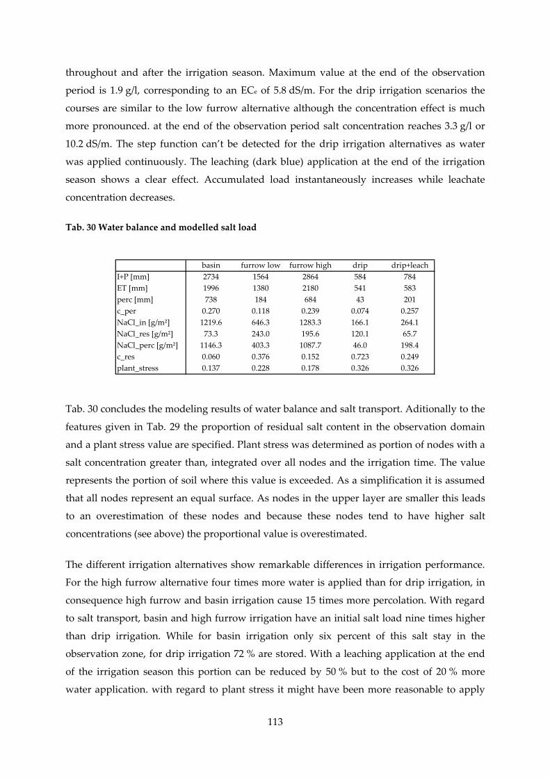
throughout and after the irrigation season. Maximum value at the end of the observation
period is 1.9 g/l, corresponding to an ECe of 5.8 dS/m. For the drip irrigation scenarios the
courses are similar to the low furrow alternative although the concentration effect is much
more pronounced. at the end of the observation period salt concentration reaches 3.3 g/l or
10.2 dS/m. The step function can’t be detected for the drip irrigation alternatives as water
was applied continuously. The leaching (dark blue) application at the end of the irrigation
season shows a clear effect. Accumulated load instantaneously increases while leachate
concentration decreases.
Tab. 30 Water balance and modelled salt load
basin furrow low furrow high drip drip+leachI+P [mm] 2734 1564 2864 584 784ET [mm] 1996 1380 2180 541 583perc [mm] 738 184 684 43 201c_per 0.270 0.118 0.239 0.074 0.257NaCl_in [g/m²] 1219.6 646.3 1283.3 166.1 264.1NaCl_res [g/m²] 73.3 243.0 195.6 120.1 65.7NaCl_perc [g/m²] 1146.3 403.3 1087.7 46.0 198.4c_res 0.060 0.376 0.152 0.723 0.249plant_stress 0.137 0.228 0.178 0.326 0.326
Tab. 30 concludes the modeling results of water balance and salt transport. Aditionally to the
features given in Tab. 29 the proportion of residual salt content in the observation domain
and a plant stress value are specified. Plant stress was determined as portion of nodes with a
salt concentration greater than, integrated over all nodes and the irrigation time. The value
represents the portion of soil where this value is exceeded. As a simplification it is assumed
that all nodes represent an equal surface. As nodes in the upper layer are smaller this leads
to an overestimation of these nodes and because these nodes tend to have higher salt
concentrations (see above) the proportional value is overestimated.
The different irrigation alternatives show remarkable differences in irrigation performance.
For the high furrow alternative four times more water is applied than for drip irrigation, in
consequence high furrow and basin irrigation cause 15 times more percolation. With regard
to salt transport, basin and high furrow irrigation have an initial salt load nine times higher
than drip irrigation. While for basin irrigation only six percent of this salt stay in the
observation zone, for drip irrigation 72 % are stored. With a leaching application at the end
of the irrigation season this portion can be reduced by 50 % but to the cost of 20 % more
water application. with regard to plant stress it might have been more reasonable to apply
113
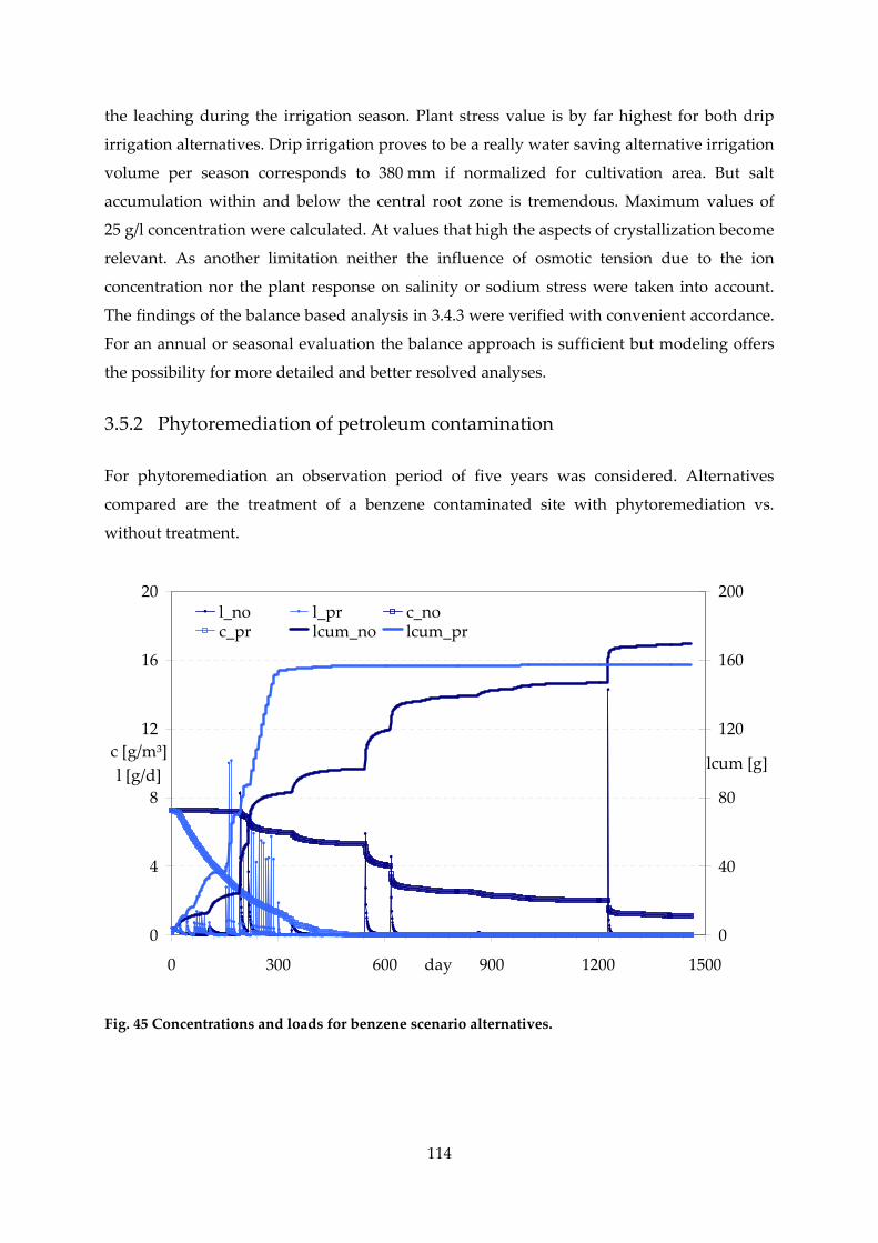
the leaching during the irrigation season. Plant stress value is by far highest for both drip
irrigation alternatives. Drip irrigation proves to be a really water saving alternative irrigation
volume per season corresponds to 380 mm if normalized for cultivation area. But salt
accumulation within and below the central root zone is tremendous. Maximum values of
25 g/l concentration were calculated. At values that high the aspects of crystallization become
relevant. As another limitation neither the influence of osmotic tension due to the ion
concentration nor the plant response on salinity or sodium stress were taken into account.
The findings of the balance based analysis in 3.4.3 were verified with convenient accordance.
For an annual or seasonal evaluation the balance approach is sufficient but modeling offers
the possibility for more detailed and better resolved analyses.
3.5.2 Phytoremediation of petroleum contamination
For phytoremediation an observation period of five years was considered. Alternatives
compared are the treatment of a benzene contaminated site with phytoremediation vs.
without treatment.
0
4
8
12
16
20
0 300 600 900 1200 1500day
c [g/m³]l [g/d]
0
40
80
120
160
200
lcum [g]
l_no l_pr c_noc_pr lcum_no lcum_pr
Fig. 45 Concentrations and loads for benzene scenario alternatives.
114
115
Fig. 45 visualizes the results of the mass transport modelling. Concentration (thin squared
line), load (thin dotted line) and accumulated load (bold line) are displayed for
phytoremediation (_pr) and no treatment scenarios (_no).
The phytoremediation site shows a continuous decrease of benzene content. Both
decomposition and washout contribute to the effect. After approximately 500 days
concentration falls below the 0.035 g/m³ concentration value, that corresponds to the limit for
agricultural use in Mendoza [Ercoli, 2001]. Accumulated load over the five year period is
158 g. For the untreated site washout clearly dominates over decomposition. For the few
drainage significant events steps as well in the load as in the concentration curves are visible,
they represent a decline of contaminant content due to losses rather than decomposition.
After the five year period the leachate of the untreated site still has a concentration of
1.3 g/m³ and continues contaminating the subjacent zone.
Residual concentration over the whole observation domain was calculated as accumulated
water content multiplied by concentration for each node, assuming the same simplification
as above. For phytoremediation alternative residual concentration was 0.2 g while for no
treatment alternative it accounted to 17.8 g or 0.74 ppm. As a conclusion, if no measure is
applied
As management recommendation poplars should not be planted in squares but in order to
provide a homogeneous root distribution throughout the soil zone. High density cultivation
as applied for biomass growth would be a feasible alternative. Additionally the high density
of plants prevents eolic soil erosion and dry deposition of the contaminant. In spite of the
percolation thread basin irrigation is recommended for phytoremediation because it
distributes water over the whole affected area. Soil humidity control should be foreseen in
order to prevent excess application and leaching of the contaminants, especially if they a well
soluble in water. Alternatively sprinkler irrigation systems could be applied.
116
4 CONCLUSIONS
This section aims to give a brief recapitulation of limitations and findings obtained
throughout the project. Results are rearranged and set into a synthesizing context so that,
without working through all the details, the central statements are at hand. Additionally
some of limitations are concluded that were not discussed within the main part as their
influence is not retraceable. Some of those factors are at the focus of fundamental research at
the moment. They are mentioned rather than discussed to put the results into a perspective
and to allow relativization for the use in other contexts.
One central point that was not emphasized in this thesis might be mentioned here: It was
quite laborious to get and keep the model running. A lot of time was spent in the
configuration of parameters that were both, exact in representation and stable in
computation. A figure might illustrate that: after all 32852 days or 90 years of time variable
boundary conditions and 125 cases were registered during the elaboration of the project,
excluding re‐runs of the same case.
4.1 Limitations 4.1.1 Data base
A lot of effort was spent on the correction, completition and interpolation of input data on
both regional and site‐scale. For many arid regions, where human activity is spread over
large extends, the lag of quantifiable information inhibits efficient solution of environmental
problems. Aside from the value for the actual project the proposal of possibilities for data
enhancement might be useful for the elaboration in similar situations of future projects.
Nevertheless the possibilities of recapitulation of lagging information were limited,
especially as the project was based on investigation done more than ten years ago.
As a clear constraint of the project it has to be marked out that neither inflow volumes nor
deep percolation rates were determined. Hence it was not possible to validate the quality of
the water balance fit. Although moisture content is a representative variable for soil water
dynamics, it integrates different effects of water movement. If e. g. moisture change at a
point is seemingly reproduced correctly it is not straightforward apparent if this is due to a
correct description of the underlying processes or due to a combination of incorrect
descriptions. Still results for the reproduction of soil moisture dynamics are satisfying in

117
calibration as well as validation. So that at least within the range of tested boundary
conditions the model can be applied as functional
The development of poplar root system for the specific varieties and site conditions of
Mendoza were not considered within this investigation. The estimates taken were basically
supported by local knowledge, however some uncertainty remains. Especially the possibility
of a hydraulic lift caused by deep sinker roots that would change completely the distribution
of roots and consequently water uptake can not be excluded.
4.1.2 Modeling
As the assumptions indicate and as it is intrinsic for modeling, simplifications had to be
applied. Some processes were not considered by the model, for some no data foundation was
available. Some main uncertainties may be concluded in the following
Boundary conditions
For the edition of boundary freedom of definition is limited. For most types of conditions
only one time series or constant value can be designated. This reduces the options to
consider a bigger model scale, e.g. for the parallel consideration of various irrigation parcels.
On a bigger scale the consideration of different climatic drivers is not possible at the
moment.
The climate type boundary condition proved very valuable to stabilize computation
procedure but the assumptions for the definition of limit values is rather conceptual than
physically based.
Water flow
For the influence of macropores and preferential flow paths is not included in the model.
These processes are occasionally important in order to represent soil moisture distribution
and infiltration properties adequately on local scale.
Surface water flow is not considered, time series may be defined to account for water levels
courses, e. g. to describe flooding but there is no interaction assumed between surface and
subsurface flow.
118
Plan growth
Although transpiration rate can be considered as a time series, the root distribution is
regarded as a steady state. Especially if long simulation periods for perennial plants are
computed this leads to unrealistic assumptions.
Interaction of plant and environment is limited. Conceptually roots are a simple sink term.
The scaling function for water uptake that is applied is widely discussed in related literature.
Especially the no continuous course and the difficulties for defining the static characteristic
suction heads are criticized. The response of roots to variable soil moisture is considered by a
single relation, this is imprecise where roots with different functionality occur. Substance
interaction between root and environment e.g. reduced consumption due to salinity stress or
the exudation of substances that support decomposition can’t be taken into account.
Analogous to the limitations for boundary conditions only a single set of root extraction
parameters can be defined. This obstructs the representation of different cultivation types or
mixed plant populations. Although to some extend the parameters can be equipped
integrally e.g. by weighting the portions of the different species, the resulting consequences
for the single species can’t be derived.
Mass transport
As already mentioned salt concentration influences via osmotic potential the total soil water
tension. The changes in water tension – water content relation for the salinity scenarios can’t
be taken into account.
At concentrations as high as the ones found for the salinization scenarios, salt crystallizes
and blocks soil pores. When rewetting the solving salts absorb water that does not contribute
to flow. The crystallization‐solution‐kinetics is a fundamental problem and influence on
water movement is not fully investigated.
Especially if the decomposition of substance mixtures, e.g. PAHs is considered the influence
of concurrence, selective decomposition, cometabolism and related effects is not fully
investigated and very case specific. For these cases the zeroth or first order decomposition
kinetics is not able to describe decomposition behavior.

119
4.1.3 Scenarios
The scenarios were set up for two purposes to validate model performance for the site
specific circumstances and to demonstrate capabilities of the application.
For all scenarios it has to be stated that it would have been desirable to incorporate more
measured data for a more adequate representation of governing processes and validation of
the results. The scenarios are set up somewhat on the merits. Especially for the
phytoremediation local experiences could not be taken into account so that the assumptions
are conceptual. Due to that the significance for actual planning is limited but the results may
raise the awareness for basic drivers and enhance system comprehension.
4.2 Findings
In this section some of the central perceptions of the work are concludes, they are not so
much oriented on the working scheme but more on different aspects of modeling and
concrete results.
4.2.1 Treatment and assessment of input data
Climate data
A strategy for the completition and regionalization of climate data was presented under
incorporation of a maximum extend of available data. Although the values measured at the
investigation site bear some uncertainties and inconsistencies they provide valuable
information about local climate effects. Especially as additional information is spatially
sparse it should be intended to account for their contribution.
Soil data
The sampling of soil was valuable for two main reasons: seemingly homogeny of the soil was
not completely confirmed. Especially grain size distribution and particle density showed
considerable variation. As a second aspect the models for the prediction of retention and
permeability properties were set into a perspective and measured data served as initial
estimate for the model calibration.
120
Soil hydraulic parameters
Both tools for the estimation of soil hydraulic parameters implemented in SiWaPro, DIN
4220 table as well as Vereecken PTF, were not able to reproduce the measured data. For the
estimation with ROSETTA only with the highest level of input data quality acceptable results
were obtained. The divergence between modeled and measured values may be partly
explained by the use of disturbed soil probes for the determination of the retention curves.
Nevertheless the systematic error does not suggest this. Generally measured water content at
equal pressure levels was lower for measured than for modeled curves although compaction
of the soil decreases the portion of big pores that drain fast at low pressure levels. Another
explanation may be that the tools implemented in SiWaPro are based on data that does not
refer to soil that evolved under arid conditions. Hence the specific properties of aridic soils
are not within the range. It should be remarked critically that the classification offered by
DIN 4220 may only serve as an orientation. The classification based only on texture classes is
not detailed enough to allow an attribution of single values for the hydraulic parameters. For
the application of ROSETTA it is recommendable to invest effort into input quality as
estimation results improved remarkably with better input data.
RETC program proved useful for the fitting of van Genuchten parameters to the measured
curve. Generally fits had small difference from measured data. Six measured points allowed
decreasing rRMSE values to less than 5 % while three measured points resulted in rRMSE
values of up to 12 %.
4.2.2 Model performance
Model performance was evaluated with a multi‐objective parameter set. The parameters
were applied for calibration and validation and allowed a comprehensive assessment on
different aspects of model performance. Additionally with the performance utility a flexible
and adaptive “metaparameter” was introduced. Its application was tested successfully.
4.2.3 Model Verification for an Arid Climate
The application of SiWaPro for an arid climate was conducted successfully. Nevertheless the
setup and calibration were laborious and readjustments were frequent in order to avoid
instabilities.
121
The combination of a soil with poor water retention, the elevated evaporation rates and
highly variable irrigation / precipitation dynamics, especially in the interannual
consideration of irrigation – non‐irrigation regimes was a challenge for the simulation tool.
Although the model configuration is not very complex, “only” a cross section of 16 x 2 m
with four trees was considered, the program proved sensitive to the elevated water
dynamics of irrigation in an arid site. The climate‐type boundary condition proved as
valuable stabilizing feature.
4.2.4 Water Balance of Poplars
It was found that in presence of trees basin irrigation induced heterogeneous patterns of soil
moisture distribution and consequently of drainage and groundwater recharge. As the
method is plane (2D) oriented water between the plant stands is applied inefficiently.
Groundwater recharge rates were high, accounting for 700 mm/a or 27 % of the irrigation
volume for seven day irrigation cycles and about 200 mm/a or 17 % for the 21 day cycle.
4.2.5 Scenarios and Best Management Recommendations
Basin irrigation is not the method of choice as irrigation practice, especially for crops where
root domain does not cover the whole irrigated subsurface. In the present case, the effect of
deep percolation is fortified by the low retention potential of the soil and the corresponding
relatively low traversal component. Irrigation water is applied efficiently if the maximum
proportion of water reaches the maximum extend of roots. As a consequence it might be
stated that “irrigation dimension” should match “crop dimension”. If trees are considered as
point crops (0D) water should correspondingly be applied on point, while for row crops
(most vegetables) should be provided by linear irrigation methods. For crops that grow
distributed over surface 2D irrigation meets plants requirements.
Furrow and drip irrigation permit to allow water much more localized and in the case of
drip irrigation timely. The problem of salt accumulation in the soil cannot be solved by these
measures but as less water is applied, also less salt is distributed. Salt accumulation for drip
irrigation exceeded tolerable values and a regular leaching has to be provided.
The plantation of hybrid poplar species that tolerate high salinity of even incorporate salt as
mentioned by [Shannon, 1998] can give a valuable contribution to cope with the salinity
thread. Although for this further investigation is necessary e. g. in order to estimate the
122
actual incorporation rates. From the present point of view drainage on field scale and a more
restrictive management of land use rights on regional scale seem to provide the most
efficient tools to reduce salinization.
4.3 Outlook
With the present work questions arose and not all aspects could be validated to a satisfying
extend. Some of the suggestions made here may stimulate interest in further projects or raise
awareness for deficits.
4.3.1 Data situation
With the emerging technologies of satellite detection for climate data and regional climate
modeling new tools for the generation and validation of measured data get available.
Although they are not yet disposable for the local scale they could at least serve as a
reference.
The base of knowledge on problems and threads for the water resources in Mendoza is
advanced. In a further step it would be relevant to take steps towards a more process
description rather than monitoring focus. This is not only a matter of will as financial
possibilities are limited but for a sustainable development and efficient decisions the
extension of coordinated and conceptual knowledge is crucial. Especially the use of remote
sensed as well as continually measured, automatically registered data could be applied to
contribute to this aspect. With regards to data acquisition concepts a water cycle oriented
approach could be favored, in a first step on local scale. E. g. the coordinated measurement of
irrigation, soil moisture, transpiration (sap flow) and drainage could contribute largely to a
better understanding of irrigation water dynamics.
4.3.2 Suggestions for model development
Many of the aspects mentioned here meet the deficits concluded in 4.1.2. They are mentioned
reviewed in order to give a more constructive feedback. The proposals from this section are
divided into two lines, some of the points focus more on additional features; others propose
adaptations in the model performance.
For the application of SiWaPro program in an agricultural context a greater flexibility in the
definition of boundary conditions would be needed. If the model is applied on a bigger scale
123
different cultivation schemes, crops and irrigation regimes occur each requiring adapted
boundary conditions. On a regional scale this option would be also interesting in order to
represent different climatic conditions. The data base approach that is used in SiWaPro for
information management favors the implementation of freely configurational boundary
condition time series but it has to be evaluated if this obstructs the intuitive use of the model
setup assistant.
Interfaces to surface runoff and groundwater models could be incorporated in order to make
SiWaPro more apt for the working field of integrated modeling. This is especially relevant
for interactive processes as the infiltration from water courses or groundwater dynamics.
Root distribution and water uptake have big influence on water movement in the soil. At the
same time the dynamics of root growth are dependent on parameters of their environment
and water availability [Mulia, 2005]. For an adequate estimation of water transport processes
it would be thus advantageous to implement time series of root parameters e. g. to represent
growth in long term simulations. In a more advanced state a root sub‐model would be
desirable that represents a growth function in interrelation with environmental boundary
conditions.
With regard to salt transport a representation of the osmotic potential would be relevant. The
connection between ion concentration and osmotic potential are described conceptually with
linear relations. For the description of crystallization‐solution‐kinetics no modeling
approaches are at hand at the moment.
4.3.3 Possible continuation
Based on the existent data an investigation on the influences of soil heterogeneity could
follow up. Soil data analysis showed a certain layering and this may lead to retaining
horizons that influence subsurface flow paths. Further data acquisition would contribute to
an enhanced accuracy as described above.
A validation under similar conditions but with measured irrigation and drainage volumes
would trigger uncertainties about the adequate process description. Especially as
irregularities in the calibration process (compare 3.3.1) were explained with uneven water
application.

124
It would be interesting to consider the drainage heterogeneity on a bigger scale. The
differences between plant – no plant points should buffer on a bigger scale but it is likely that
configuration of plant positions, crop types and soil properties do have a mentionable
influence.
For the phytoremediation a feasibility study would be valuable. Although a lot of
investigation is done in the field of bioremediation, this technique is not considered yet.
Based on local knowledge experience design, management and control could be supported
by an accompanying model approach.

125
5 QUELLENVERZEICHNIS
Abihaggle C. E., Day J. A.: Agua y sociedad: un ensayo económico sobre la política hídrica;
EDIUNC; Mendoza; 2004
Abraham M. E.: Mapa Geomorphologico de Mendoza Sector Norte; Catálogo de Recursos
Humanos e Información Relacionada con la Temática Ambiental en la Región Andina
Agrentina; Abraham E. M., Martínez F. R. (Edt.); C‐Bra Systematics; Buenos Aires; 1999
Abrahamson D. A. et al.: Calibration of the Root Zone Water Quality Model for Simulating
Tile Drainage and Leached Nitrate in the Georgia Piedmont; Agronomy Journal; Vol. 97
(2005); p. 1584–1602.; American Society of Agronomy
AG Boden: Bodenkundliche Kartieranleitung; Publ.: Bundesanstalt für Geowissenschaften
und Rohstoffe und Geologische Landesämter; 4. Edt.; Hannover; 1994.
Allen R. et al.: Crop evapotranspiration ‐ Guidelines for computing crop water requirements;
FAO Irrigation and drainage paper 56; FAO (Food and Agriculture Organization of the
United Nations); Rome; 1998
Aragüés R. et al.: Conceptual irrigation return flow hydrosalinity model; in: Agricultural
salinity assessment and management; Tanji K. K. (Edt.); ASCE Manuals and Reports on
Engineering Practices No. 71; American Society of Civil Engineers; New York; 1990
Austenat L., Zink C.: Handbuch Stoffdaten zur Störfall‐Verordnung : Zusammenstellung von
Informationen zu Stoffeigenschaften und zum Reaktionsverhalten gefährlicher Chemikalien;
Umweltbundesamt (Edt.); Schmidt; Berlin; 1986
Ayers R. S., Westcot D. W.: Water quality for agriculture;. Irrigation and Drainage Paper; No.
29, Rev. 1; FAO (Food and Agriculture Organization of the United Nations) (Edt.); Rome;
1985
Baars E., van Logchem B.P.: A client‐oriented and quantifiable approach to irrigation design,
a case‐study in Mendoza, Argentina; DLO Winand Staring Centre; Report 75.1; Wageningen;
1993
Becerra L. C. G. et al.: Ciencias Sociales Mendoza; Santillana; 1st Edt.; Buenos Aires; 2007
126
Bergemann M.: Berechnung des Salzgehalts der Elbe; Arbeitsgemeinschaft Reinhaltung der
Elbe, Wassergütestelle Elbe (Edt.); Hamburg; 2005
Benson C. H.: Springer Proceedings in Physics; Theoretical and Numerical Unsaturated Soil
Mechanics; Vol. 113; Springer; Berlin, Heidelberg; 2007
Blankenburg R. et. al: SiWaPro DSS software program;
Blankenburg R. et al.: Programmdokumentation SiWaPro; KP Ingenieurges. für Wasser und
Boden mbH, TU Dresden; 2007
Bloch G.: Irrigación distiguió a otra empresa que preserva el ambiente; B&T Gerencia
Vitivinícola; No. 4, Mendoza; 2000
Borg H: The Relationship Between the Concentration of Total Soluble Salts and Osmotic
Potential in Soil, Ground and Surface Waters for Several Regions of Western Australia;
Resource Management Technical Report No.83; Department of Agriculture Western
Australia; Perth;2001
BMZ (Bundesministerium für Zusammenarbeit) (Edt.): Environmental Handbook Volume
III: Compendium of Environmental Standards; Vieweg; Eschborn; 1995
Borsdorf A. C., Hofert H.: Naturräume Lateinamerikas: Von Feuerland bis in die Karibik.;
LAS‐Online; Österreichisches Lateinamerika‐Institut (www.lateinamerika‐studien.at/
content/natur/natur/natur‐titel.html); Wien; 2003
Bos M. G., Chambouleyron J. L. (Edts.): Parámetros de Desempeño de la Agricultura de
Riego de Mendoza, Argentina; Internacional Water Managment Institute, Latin America
Series; Vol. 5; Battaramulla; 1997
Bouwer C., Heibloem M: Irrigation Water Needs; FAO Irrigation Water Management
Training Manual no. 3; FAO (Food and Agriculture Organization of the United Nations);
Rome; 1986
Boyer J. S.: Plant Productivity and Environment; Science; Vol. 218. No. 4571; p. 443 – 448;
American Association for the Advancement of Science; New York; 1982
127
Burns R. M. et al. (Edts.): Silvics of North America: Vol. 2. Hardwoods; Agriculture
Handbook 654; U.S. Department of Agriculture; Forest Service; Washington DC; 1990
Bustamante J. A.: Proyecto – Cultivo de forestales en cortas rotaciones para la producción de
biomasa; Programa Jornada Cultivos energéticos en la región de Cuyo; Facultad de Ciencias
Agrarias, UNCuyo; Mendoza; 09.05.2008
Calderón A. D.: Silvicultura y situación de álamos en Cuyo; Actas Jornadas de Salicáceas
2006; p. 71‐79; Buenos Aires; 2006
Chambouleyron L. J.: Irrigation and Remote Sensing in the Province of Mendoza, Argentina;
in Menenti M. (Ed.): Remote Sensing and Management of Irrigation; Centro Regional Andino
(INCYTH); Mendoza; 1990
Chambouleyron L. J. et al.: Descripción y balance hídrico salino; in: Conflictos ambientales en
tierras regadías: Evacuación de impactos en la cuenca del río Tunuyán Mendoza, Argentina;
Chambouleyron J. et al. (Edts.); UNCuyo; Mendoza, 2002
Chappell J.: Phytoremediation of TCE using Populus; Status Report; U.S. EPA Technology
Innovation Office; Washington D.C.; 1997
Collins C. D.: Implenting Phytoremediation of Petroleum Hydrocarbons; in:
Phytoremediation – Methods and Reviews; Neil Willey (Edt.); Humana Press; Totowa, (NJ);
2007
Corripio J. et al.: Modeling climate‐change impacts on mountain glaciers and water resources
in the Central Dry Andes; in: Darkening Peaks: Glacier Retreta; Orlove B. et al. (Edts.); p. 126‐
135; Science and Society; University of California Press; San Diego; 2007
DEIE (Dirección de Estadísticas e Investigaciones Económicas) (Edt.): Estadísticas
agropecuarias. Uso de la tierra.; Gobierno de Mendoza; Mendoza, 2001a
DEIE (Dirección de Estadísticas e Investigaciones Económicas) (Edt.): Censo de Población y
Vivienda; Gobierno de Mendoza; Mendoza, 2001b
DEIE (Dirección de Estadísticas e Investigaciones Económicas) (Edt.): Síntesis Estadística
Social y Económica de la Provincia de Mendoza; Gobierno de Mendoza; Mendoza, 2007

128
DGI (Departamento General de Irrigación) (Edt.): Presupuestos de Gastos y Cálculo de
Recursos de las Inspecciones de Cauce de la Provincia; DGI; Mendoza; 1994
DGI (Edt.): Proyecto PNUD‐FAO‐ARG‐00/08 Informe General – Unidad de SIG y
Teledetección; DGI; Mendoza; 2003
DGI (Departamento General de Irrigación) (Edt.): Política provincial de riego – Marco legal e
institucional; DGI; Mendoza; 2005
DGI (Departamento General de Irrigación) (Edt.):Pronóstico de escurrimiento periodo
Octubre 2006 ‐ Septiembre 2007; DGI; Mendoza; 2007a
DGI (Departamento General de Irrigación) (Edt.): Plan de Recursos Hídricos; Proceedings of
Taller Provincial ‐ Plan de Recursos Hídricos; DGI; Mendoza; 27.02.2007b
DIN (Deutsches Institut für Normierung) (Edt.): DIN 4220 – Kennzeichnung, Klassifizierung
und Ableitung von Bodenkennwerten (normative und nominale Skalierungen); Beuth Verlag
GmbH; Berlin; 2007
DIN (Deutsches Institut für Normierung) (Edt.): DIN 18128 – Baugrund ‐ Untersuchung von
Bodenproben ‐ Bestimmung des Glühverlustes; Beuth Verlag GmbH; Berlin; 2007
DIN (Deutsches Institut für Normierung) (Edt.): DIN 18130 – Baugrund ‐ Untersuchung von
Bodenproben; Bestimmung des Wasserdurchlässigkeitsbeiwerts ‐ Teil 1: Laborversuche;
Beuth Verlag GmbH; Berlin; 1998
Dixon J.: An Evaluation of Unsaturated Flow Models in an Arid Climate; Thesis Master of
Science Degree; Howard R. Hughes College of Engineering; Las Vegas; 1999
Dogan A., Motz L. H.: Saturated‐Unsaturated 3D Groundwater Model; Journal of
Hydrologic Engineering; Vol. 10 (2005) No. 6; p. 505‐515; ASCE (American Society of Civil
Engineers); Reston (VA)
Doty S. et al.: Enhanced phytoremediation of volatile environmental pollutants with
transgenic trees; Proceedings of the National Academy of Sciences of the United States of
America; p.16816–16821; National Academy Press; Washington; 2007

129
DVWK (Deutscher Verband für Wasserwirtschaft und Kulturbau): Fallbeispiel zur
Nutzwertanalyse – Wasserwirtschaftliche Planung Emstal; Mittelungen; Vol. 23;Köln; 1993
Dyck S., Peschke G.: Grundlagen der Hydrologie; Verlag für Bauwesen; 3rd. Edition; Berlin;
1995
Eisenführ F, Weber M.: Rationales Entscheiden; Springer; Berlin, Heidelberg; 1993
Ercoli E. et al.: Analisis sobre la aplicabilidad de tecnicas biologicas en tratamiento de suelos
contaminados con hidrocarburos pesados; technical report; unpublished, 2001
Ercoli E.: Problemática ambiental generada por el uso de emulsión inversa en perforación
petrolera; 6tas Jornadas de Preservación de Agua, Aire y Suelo en la Industria del Petroleo y
del Gas; Instituto Argentino deletroleo y del Gas; Neuquen; 31.10 – 02.11.2005a
Ercoli, Eduardo et al.: Clean up practical limits on full scale bioremediation processes for
hydrocarbon contaminated soils; Proceedings of the 20th International Conference on Solid
Waste Technology and Management; Department of Civil Engineering, Widener University;
Chester (PA); 3.–6.04.2005b
FAO (Food and Agriculture Organization): Reforming Water Resources Policy. A Guide to
Methods, Processes and Practices; FAO Irrigation and Drainage Paper; No. 52.; Rome; 1995
FAO (Food and Agriculture Organization): World Reference Base for Soil Recourses; World
Soil Recourses Report; International Soil Science Service; Rome; 2006
Fasciolo G. et al.: Evaluación del impacto ambiental en acuíferos: contaminación producida
por actividades de saneamiento y disposición de efluentes; Proyecto; Taller sobre hidrología
de áreas regadías; Instituto Nacional de Agua Centro Regional Andino; Mendoza; 17.11.2006
Feddes R. A. et al.: Simulation of Field Water Use and Crop Yield; John Wiley & Sons; New
York; 1978
Feddes R. A. et al.: Modeling Root Water Uptake in Hydrological and Climate Models;
Bulletin of the American Meteorological Society; American Meteorological Society; Vol. 78
(2001); p. 2797 – 2809; Redwood

130
Fiorenza S. et al.: Phytoremediation of Hydrocarbon‐Contaminated Soils; CRC; Boca Raton
(Fl); 1999
Foster S., Garduño H.: Argentina – Integrated Approaches to Groundwater Resource
Conservation in the Mendoza Aquifers; Sustainable Groundwater Management: Concepts
and Tools ; World Bank Global Water Partnership Associate Program; No. 6; New York, 2005
Frick C. M. wt al.: Assessment of Phytoremediation as an In‐Situ Technique for Cleaning Oil‐
Contaminated Sites; Project Report; Department of Soil Science, University of Saskatchewan;
Saskatoon; 1999
Friend L. A. et al.: Quantification of two‐year‐old hybrid poplar root systems: morphology,
biomass, and 14C distribution; Tree Physiology; p. 109‐119; Heron Publishing; 1991
Gerbi B. et al.: Geology and structural history of the southwest Precordillera margin,
northern Mendoza Province, Argentina; Journal of South American Earth Sciences; Vol. 14;
p. 821 – 835; Pergamon; Oxford; 2001
Gielen B., Ceulemans R.: The likely impact of rising CO2 on natural and managed Populus: a
literature review; Environmental Pollution; Vol. 115 (2001); p. 335‐358; Elsevier; Amsterdam
Giraud Billou C.: Informe final sobre Estudios de Distribución del Agua – Proyecto
Constitución y Montecaseros; Departamento General de Irrigación; Mendoza; 2001
Gómez‐Silva B. et al.: Atacama Desert Soil Microbiology; in: Microbiology of Extreme Soils;
Dion P., Nautiyal C. S. (Edts.); Springer; Berlin, Heidelberg; 2008
Grassi J. C.: Aspectos metodológicos, para la determinación experimental de la evaporación
y la frecuencia de riego; CIDIAT (Centro Interamericano de Desarrollo e Investigación
Ambiental y Territorial); Material Didáctico de Riego y Drenaje No. 26; Merida; 1978
Gudiño de Muñoz M. E.: Problemática de la agricultura periurbana: caso oasis del Río
Mendoza; Boletín de Estudios Geográficos; No. 24/87; Universidad Nacional de Cuyo;
Mendoza; 1991
Hernández J. u. Martinis M.: Particularidades de las Cuencas Hidrogeologicas explotadas
con fines de Riego en la Provincia de Mendoza; III Jornadas de Actualización en Riego y
Fertirriego; Instituto Nacional de Tecnología Agropecuaria ;Mendoza; 10.‐11.08.2006a
131
Hernández, J. et al: Aplicación del modelo de flujo de aguas subterraneas MODFLOW al
acuífero de la subcuenca El Carrizal y su extensión al oasis norte; Taller sobre hidrología de
áreas regadías; Mendoza; 17.11.2006b
Hoffmann J., Viedt H.: Biologische Bodenreinigung; Springer; Berlin, Heidelberg; 1998
Hopmans J. W., Stricker J. N. M.: Stochastic analysis of soil water regime in a watershed;
Journal of Hydrology; Vol. 105 (1989); p.57‐84; Elsevier; Amsterdam
Howell R. A., Evett S. R.: The Penman‐Monteith Method; USDA Agricultural Research
Service; Bushland; 2004
Hsieh P. A. et al. (Edts.): Conceptual Models of Flow and Transport in the Fractured Vadose
Zone; Panel on Conceptual Models of Flow and Transport in the Fractured Vadose Zone;
National Academy Press; Washington; 2001
INDEC (Instituto Nacional de Estadísticas y Censos): Censo Nacional de Población, Hogares
y Viviendas del año 2001; INDEC; Buenos Aires, 2002
INDEC (Instituto Nacional de Estadísticas y Censos): Proyecciones provinciales de población
por sexo y grupos de edad. 2001‐2015; Serie Análisis Demográfico; No. 31; INDEC; Buenos
Aires, 2005
ISO (International Standardization Organisation) 10390: Soil quality ‐ Determination of
Determination of pH; International Organization for Standardization; Geneva; 1994
ISO (International Standardization Organisation) 11272: Soil quality ‐ Determination of dry
bulk density; International Organization for Standardization; Geneva; 1998
ISO (International Standardization Organisation) 11277: Soil quality ‐ Determination of
particle size distribution in mineral soil material ‐‐ Method by sieving and sedimentation;
International Organization for Standardization; Geneva; 1998
ISO (International Standardization Organisation) 11461: Soil quality ‐ Determination of soil
water content as a volume fraction using coring sleeves ‐ Gravimetric method; International
Organization for Standardization; Geneva; 2001

132
Jensen M.E. et al.: Evaporation and irrigation water requirements; ASCE Manuals and
Reports on Eng. Practices No. 70; Am. Soc. of Civil Eng., New York; 1990
Jordahl J. L. et al.: Effect of hybrid poplar trees on microbial populations important to
hazardous waste bioremediation; Environmental Toxicology and Chemistry; Vol. 16 No.6; p.
1318‐1321; Allen Press; Lawrence (KS); 1997
Kavazanjian E. et al.: Unsaturated Flow Flux Assessment for Evapotranspirative Cover
Compliance; in: Unsaturated Soils 2006 ‐ Proceedings of the Fourth International Conference
on Unsaturated Soils; Miller G. A. et al. (Edts.); Carefree; 02.–06.04.2006
Keese K. E. et al.: Assessing controls on diffuse groundwater recharge using unsaturated
flow modeling, Water Resources Research; Vol. 41; American Geophysical Union;
Washington; 2005
Kemmesies O.: Darstellung des Sachstandes, Umsetzung im Programm SiWaPro/HYDRUS;
BWK‐AG 6.2 „Instrumente zur Sickerwasserprognose“; BWK‐Materialien; 1999
Klinka K. et al.: Distribution and Synopsis of Ecological and Silvical Characteristics of Tree
Species of British Columbia’s Forests; Forest Sciences Department, University of British
Columbia; Coquitlam BC: Canadian Cartographics Ltd; Vancouver; 2000
Leiva J. C. et al.: 20 years of mass balances on the Piloto glacier, Las Cuevas river basin,
Mendoza, Argentina; Global and Planetary Change; Vol. 59; p. 10–16; Elsevier; Amsterdam;
2007
Leguizamón G. et al.: Sistemas productivos agroforestales adaptados a pequeños
productores del área de riego salinizada de Santiago del Estero; in: Cáceres, Daniel M.:
Catálogo de tecnologías para pequeños productores agropecuarios 2; Secretaría Agricultura,
Ganadería, Pesca y Alimentación; Buenos Aires ; 2007
Li Y. et al.: Root‐Water‐Uptake Based upon a New Water Stress Reduction and an
Asymptotic Root Distribution Function; Earth Interactions; Vol. 10 (2006) No. 14 ; p 1‐22;
http://EarthInteractions.org; Wisconsin
LUBW (Landesanstalt für Umweltschutz Baden‐Württemberg)(Hrsg.): Arbeitsanleitung
Pegel und Datendienst – Durchflussermittlung mit der Salzverdünnungsmethode;
Karlsruhe; 2002

133
Luckner, L., van Genuchten, M.Th., Nielsen, D.R.: A Consistent Set of Parametric Models for
the Two‐Phase Flow of Immiscible Fluids in the Subsurface; Water Resources Research; Vol.
25(10), 1989; p. 2187‐2193; Elsevier; Amsterdam
Maddock T. et al.: The overview of atmospheric and surface water coupling to regional
groundwater models in semi‐arid basins; American Meteorological Society ‐ Special
Symposium on Hydrology; Phoenix; 1998
Marre M. et al.: Irrigation water rates in Mendoza’s decentralized irrigation administration;
Irrigation and Drainage Systems 12: 67–83, Kluwer; Amsterdam; 1998
Mastrantonio L. et al.: Variación espacio‐temporal de características edáficas y paisajísticas
en un sistema bajo riego; Presentación Facultad Ciencias Agrarias Universidad Nacional de
Cuyo; Mednoza; 2006
MdR (Municipalidad de Rivadavia): Sistema de Información Geográfica Municipal; MdR;
Rivadavia; 2008
Mendieta M: En LatAm, incluida la Argentina consumimos el doble de agua que en Europa o
Estados Unidos; El Informatorio; 21.03.2007; Madrid
Menenti M. (Edt.): Mecanismos de aprovechamiento hídrico en la región andina – Modelos
de simulación e imágenes satelitarias; Centro Regional Andino‐Instituto Nacional de Ciencia
y Técnicas Hídricas; Mendoza; 1988
Menenti M.: Analysis of regional water resources and their management by means of
numerical simulation models and satellites in Mendoza, Argentina; Modelling and
Management of Sustainable Basin‐scale Water Resource Systems; International Association
of Hydrological Sciences; Publication No. 231; Boulder; 1995
Mirábile C.: Estudio Zonal de Drenaje del Río Tunuyán Medio. Diez Anos de Control
Freatimétrico; INA‐CRA (Instituto Nacional de Agua‐Centro Regional Andino; Mendoza;
1997
Mirábile C. et al.: Dinámica de la salinidad del Suelo en el Oasis del Río Tunuyán Inferior
Comparación 1985 – 2002; INA‐CRA (Instituto Nacional de Agua‐Centro Regional Andino;
Mendoza; 2003
134
Mirábile C. et al.: Validación del modelo hídrico‐salino “Balansal” en suelos cultivados de la
Pampa Húmeda cultivados con riego complementario; Presentation; Proyecto de
Investigación y Desarrollo; Ministerio de Planificación Federal, Inversión Publica y Servicios,
Subsecretaría de Recursos Hídricos; Buenos Aires; 2006
Montes T. A.: El proyecto Potrerillos; Diario Uno; Mendoza; 29.10.1995
Montaña E. et al.: Coming Down the Mountain: Understanding the Vulnerability of Andean
Communities to Hydroclimatologic Variability and Global Environmental Change; Inter‐
American Institute for Global Change Research; Sao Paolo; 2008
Moormann H.: Einfluss der Rhizodeposition von Helophyten auf den mikrobiellen
Schadstoffabbau; UFZ‐Bericht; No. 1/2002; Halle, Leipzig; 2002
Morábito J. et al.: Salinidad de Suelos Regadíos e Incultos en el Oasis Norte de Mendoza –
Argentina; INA‐CRA (Instituto Nacional de Agua‐Centro Regional Andino; Mendoza; 2005
Morábito J. et al.: Determinación de escenarios de la demanda de riego en el área dominada
por el Río Mendoza; Convenio Instituto Nacional del Agua y Ministerio de Ambiente y
Obras Públicas del Gobierno de la Provincia de Mendoza (Resolución Nº 1984/00), Informe
Final; INA‐CRA (Instituto Nacional de Agua‐Centro Regional Andino; Mendoza; 2004
Morábito J. et al.: Using performance indicators for the analysis of water use in the Mendoza
irrigated area; in: Sustainabiltiy of Groundwate recouses and its indicators – Proceedings of
the Seventh IAHS Scientific Assembly at Foz do Iguaçu; IAHS Publishing; 2006
Mualem Y.: A New Model for Predicting the Hydraulic Conductivity of Unsaturated Porous
Media; Water Resources Research; Vol. 12 1976(3); p. 513‐522; Elsevier; Amsterdam
Mulia R., Dupraz C.: Unusual 3D fine root distributions of two deciduous tree species
observed in Southern France: what consequences for root dynamics modelling?; INRA
Montpellier; unpublished; 2005
Neumann R. et al.: Stress physiology of poplars – abiotic factors; in: Biology of Populus and
its Implications for Management and Conservation; Stettler R. et al. (Edts.); NRC Research
Press; Ottawa; 1996
135
Nielsen D. R., Luckner L.: Theoretical aspects to estimate reasonable initial parameters and
range limits in identification procedures for soil hydraulic properties; Proceedings of the
International Workshop on Indirect Methods for Estimating the Hydraulic Properties of
Unsaturated Soils (M. Th van Genuchten et al.); University of California; Riverside; 1992
Nijensohn L.: Curso de Edafología V‐1 “El suelo como sistema polifásico heterogéneo”,
Edición C.E.F.C.A., Mendoza; 1962a
Nijensohn L., Pilasi H.: Correlación entre contenido de agua a pF0, volumen de
sedimentación y porcentaje de arcilla; Resúmenes de Trabajos y Comunicaciones, 2da
Reunión Argentina y 1er Congreso Latinoamericano de la Ciencia del Suelo, Mendoza; 1962b
Ongay O., Bourget M.: Curso de educación ambiental – 10 flora; Gobierno de Mendoza,
Ministerio de Ambiente y Obras Públicas, Subsecretaría de Medio Ambiente, Programa
Provincial de Educación Ambiental; Mendoza; 2006
Ogg C. M. et al.: Statistical Verification of Soil Discontinuities in Virginia; Soil Science;
Lippincott, Williams & Wilkins; Philadelphia, 2000
Ortíz Maldonado G. et al.: Salinidad en el agua freática regadía en el área del Río Mendoza;
Revista de la Facultad Ciencias Agrarias Universidad Nacional de Cuyo; Vol. 37 (2005), Nr.
2; p. 51 – 64; Mendoza
OSM (Obras Sanitarias de Mendoza): Consumo de agua en el área de la ciudad de Mendoza;
OSM; Mendoza; 1996
Peyke G., Schneider T.: Mendoza – Stadt und Oase am Fuße der Anden: Beiträge zur
regionalen Geographie des argentinischen Westens; Geographisches Institut der Humboldt
Universität Berlin; Berliner Geographische Arbeiten; No. 85; Berlin; 1998
Pilipovych A. et al.: Investigating potential of some poplar clones for phytoremediation of
nitrates through biomass production; International Poplar Commission; Conference:
Environmental Applications of Poplar and Willow Working Party; Northern Ireland; 18‐
20.05.2006
Pregitzer K. S., Friend A.L.: The Structure and Function of Populus Root Systems; in: Biology
of Populus and its Implications for Management and Conservation; Stettler R. et al. (Edts.);
NRC Research Press; Ottawa; 1996

136
Querner E. P., Bakel v. P.: Description of the regional groundwater flow model SIMGRO;
Report 72 DLO; The Winland Staring Centre; Wangeningen; 1988
Querner E. P. et al.: The use of hydrological models in the irrigated areas of Mendoza,
Argentina; Agriculutral Water Management; Vol. 35 (1997); p. 11‐28; Elsevier; Amsterdam
Querner E. P. et al.: SIMGRO, a GIS‐Supported Regional Hydrologic Model in Irrigated
Areas: Casa Study in Mendoza, Argentina; Journal of Irrigation and Drainage Engineering;
Vol. 134 (2008); Nr. 1; p. 43 – 48; ASCE (American Society of Civil Engineers); Reston (VA)
Riu N.: Evaporación actual por capa diagnostica en álamos de 5 años edad; unpublished
data; Mendoza; 1993
Riu N., Settepani V.: Requerimiento hídrico en álamos de 6 años Rivadavia, Mendoza
(Argentina); Revista de la Facultad Ciencias Agrarias Universidad Nacional de Cuyo; Vol. 36
No. 1; p. 63 – 68; Mendoza; 2004
Riu N., Settepani V.: Requerimiento hídrico en álamos de 5 años Rivadavia, Mendoza
(Argentina); Revista de la Facultad Ciencias Agrarias Universidad Nacional de Cuyo; Vol. 35
No. 1; p. 52 – 57; Mendoza; 2003
Riu N: personal correspondence, May – Sept. 2008a
Riu N: Fertirrigación en álamos de 6 años de edad; Revista de la Facultad Ciencias Agrarias
Universidad Nacional de Cuyo; submitted; Mendoza; 2008b
Rodríguez Aguilera P. et al.: Estudio para el control de inundaciones en el área de afectación
del canal cacique Guaymallen; Departamento General de Irrigación; Mendoza; 2006
Roig F. A. et al..: Mapa de Vegetación de la Provincia Mendoza; Catálogo de Recursos
Humanos e Información Relacionada con la Temática Ambiental en la Región Andina
Agrentina; Abraham E. M., Mertinez F. R. (Edt.); C‐Bra Systematics; Buenos Aires; 1999
Roig F. A.: Bosquejo fisionómico de la vegetación de la provincia de Mendoza; ECOSUR; Vol.
3; p. 1 – 45; Rosario; 1972
137
Rojas J. F.: La Justicia investiga una contaminación petrolera próxima a El Carrizal;
http://www.argenpress.info/2008/11/argentina‐mendoza‐la‐justicia‐investiga.html; visited
10.12.2008; 05.11.2008
Rydberg Z: Course on Phytoremediation; Department of Biology, Colorado State University;
http://rydberg.biology.colostate.edu/CourseCatalog/syllabus/FA03.pdf; visited 08.12.2008;
2003
SAGPyA (Secretaria de Agricultura, Ganadería, Pesca y Alimentos): Sector Forestal – Año
2006; Dirección de Producción Forestal, SAGPyA; Buenos Aires; 2007
Salomon M. A. et al.: Estimación del Balance Hídrico mediante aplicación des modelo
ISAREG en el canal Segundo Visalba Lujan de Cuyo. Mendoza (Argentina); Taller
ʺModernización de riegos y uso de tecnologías de la informaciónʺ La Paz; 17‐19.09.2007
Schaap M., Leij F. J.: Improved Prediction of Unsaturated Hydraulic Conductivity with the
Mualem‐van Genuchten Model; Soil Science Society of America Journal; Vol. 64; p. 843‐851;
Soil Science Society of America; Stanford; 2000a
Schaap M.: ROSETTA model for estimation of unsaturated hydraulic soil properties; version
1.2; US Salinity Service, Riverside; 2000b
Scheimberg S.: Petroleo y Gas sus Aportes a la Argentina; Instituto Universitario ʹEscuela
Superior de Economía y Administración de Empresasʹ; Concurso de ensayos en
conmemoración a los 100 anos del descubrimiento de petróleo en Argentina; Buenos Aires,
2007
Schmitz G. et al: Irrigation control: towards a new solution of an old problem; IHP/HWRP‐
Berichte; No. 5; Hydrology and Water Resources Programme of WMO; Koblenz; 2007
Schnoor, J. et al.: Phytoremediation of organic and nutrient contaminants; Environmental
Science and Technology; Vol. 29 No. 7; p. 318‐323; American Chemical Society Publications;
Washington D.C.;1995
Šimunek J. et al.: The SWMS_2D code for Simulating the Two‐Dimensional Movement of
Water, Heat, and Multiple Solutes in Variably‐Saturated Media, Version 1.1.; Research
Report No.132; US. Sa1inity Service; Riverside; 1994;
138
Šimunek J. et al.: STANMOD Studio of Analytic Models for Solving Convection Dispersion
Equation; version 2.2; US Salinity Service, Riverside; 1998
Šimunek J. et al.: The HYDRUS‐2D Software Package for Simulating the Two‐Dimensional
Movement of Water, Heat, and Multiple Solutes in Variably‐Saturated Media, Version 2.0;
Research Report No.132; US. Sa1inity Service; Riverside; 1994;
Sivera M: Petróleo y Gas: Petróleo: La mitad de la industria de Mendoza; Diario de los
Andes; Mendoza; 24.03.2003
Shannon M. C., Banuelos G. S.: Poplars that cope with salty water, Agricultural Research;
Volume 28 ; p. 19; USDA; Washington; 1998
Stuwort M.: Suck it up – also known as Phytoremediation; in: Our garden gang – In the
garden; online‐publication www.ourgardengang.com/pubs/inthegarden.html; 2003
Thomas P. Oasenbewässerung in Trockenräumen: Ansichten zum Problem des
Managements von Bewässerungswasser und Einzugsgebieten am Beispiel der äprovinz
Mendoza – Argentinien; in: Mendoza – Stadt und Oase am Fuße der Anden: Geographie des
argentinischen Westens; Peyke G, Schneider T. (Edts.); Geographisches Institut der
Humboldt Universität Berlin; Berliner Geographische Arbeiten; Vol. 85; Berlin; 1998
Thomas Z. et al.: Simulating soil‐water movement under a hedgerow surrounding a
bottomland reveals the importance of transpiration in water balance; Hydrological Processes;
Volume 22 (2008), Nr. 5, p. 577 – 585
Torre V.: El Algarrobo; Editorial Dunken; Buenos Aires; 2006.
Trapp S. Phytoremediation organischer Schadstoffe; Umweltwissenschaften und
Schadstoffforschung; Vol. 12, No. 5; p. 246‐255; 2000
Trapp S., Karlson U.: The effect of Phytoremediation of Organic Pollutants; Journal of Soil
and Sediments; Vol. 1; p. 1‐7; Ecomod; Landsberg; 2001
Tschaplinski T. J. et al.: Drought resistance of two hybrid populus clones in a large scale
plantation ; Tree Physiology ; Volume 18 (1998) ; p. 653‐658
139
USDA (United States Department of Agriculture) (Edt.): Soil Taxonomy; 2nd Edition;
Agriculture Handbook No. 436; USDA; Washington; 1999
van Genuchten, T. M. (1980): A Closed‐form Equation for Predicting the Hydraulic
Conductivity of Unsaturated Soils; Soil Scientific Society of America (ASSS) Journal; 44
(1980); p. 892‐898; ASSS
van Genuchten T. M. et al.: RETC Code for Quantifying the Hydraulic Functions of
Unsaturated Soils; version 6.0; US Salinity Service, Riverside; 2002
Velasco M. I.: Los aprovechamientos de agua para riego en la región árida argentina; Boletín
de Estudios Geográficos; Vol. 7; UN Cuyo; Mendoza; 1963
Ventosa A. et al.: Halophytic and Halotolerant Micro‐Organisms from soils; in: Microbiology
of Extreme Soils; Dion P., Nautiyal C. S. (Edts.); Springer; Berlin, Heidelberg; 2008
Vereecken H. et al.: Estimating the soil moisture retention characteristics from texture, bulk
density and carbon content; Soil Science; Vol.148 ((1989), p. 389‐403; USDA; Washington D.C.
Verstraeten W. W. et al: Comparative analysis of the actual evapotranspiration of Flemish
forest and cropland, using the soil water balance model WAVE; Hydrology and Earth
Sciences; No. 2 (2005); p. 761‐799;
Willmott C.J. et al.: Statistics for the evaluation and comparison of models; Journal of
Geophysical Research; Vol. 90; p. 8995‐9005; Elsevier; Amstedam; 1985
Yeh, G. T. Tripathi, V. S.: HYDROGEOCHEM‐ A coupled model of hydrologic transport and
geochemical equilibria in reactive multicomponent systems; Environs Science Division, Publ.
No.3170; Oak Ridge National Lab.; Oak Ridge; 1990
Zhang J. et al.: Effects of salinity stress on poplars seedling growth and soil enzyme activity;
Silviculture and Forestry; 16(2005), Nr. 3; p. 426‐30; Beijing
Top Related