


Languages
Pages
Legal

DIGITAL FILTERING
AhD ACCELERATION PULSE INTERPRETATION
E. L. Fasanella
PRC Kentron, Inc.
Aerospace Technologies Division
Hampton, Virginia
NASA/FAAGovernment/IndustryCID _brkshop
NASA Langley Research Center
April i0, 1985
103
https://ntrs.nasa.gov/search.jsp?R=19860012470 2018-07-02T09:08:11+00:00Z

TOPICS
This presentation will address digital filtering of the CID data and atechnique to analyze the acceleration data (fig. I). Analog filtering wasperformed by electronic hardware (low pass analog filters) on board theaircraft to remove undesired high frequencies and to prevent errors due tosampling. Digital filtering is a computerized post-processing filteringtechnique that can be applied to the digitized time history data. Low pass,high pass, and notch filters can be mathematically simulated with this ,technique.
In order to validate acceleration traces, the integrated crash pulsevelocity change was computed. Traces with velocity change outside theexpected envelope were either rejected or set aside for additional study.Average accelerations were computed by dividing the primary impact velocitychange by the pulse duration. An equivalent triangular pulse accelerationwas computed by doubling the average acceleration and this value wascompared to peak acceleration values. Selected traces were chosen that
illustrate the effects of digital filtering for structure and dummyoccupants. Other traces were chosen to illustrate the method used to obtain
the average pulse acceleration and to triangularize the acceleration pulse.
• Digital filtering
• Digital versus analogfiltering
• Data interpretation
• Peakand averageaccelerations
• Velocity
• Triangularizing the accelerationpulse
• Discussionof selecteddatatraces
Figure 1
104

SAE CLASS 60 FILTER
A low pass filter with frequency response that lies within the innerand outer limits sh_n by the solid straight lines is defined by SAE J211a(ref. I) to be a class 60 filter. The digital filter chosen to smooth CIDaccelerometer data is shown on figure 2 by a dashed line. The digital
filter is flat with no attenuation (0 decibels) to the cutoff frequency fcand then rolls off until it attenuates all frequencies above the terminal
frequency ft" This digital filter with fc = I0 Hz and ft = 188 Hz will be
designated henceforth as the CID 100-Hz digital filter.
2 - ClD 100Hzdigital filter Outer limit0-- ---_ "_/-
-4- x\ Digitalfilter
-6 - Inner limit fc 10Hz
,o- /', \Decibels ft = 188Hz
-15 - I _-20 -
-25 I I I I•1 1.0 10 100 1000
Logfrequency, Hz
Figure 2
I05

DIGITAL FILTERING EXAMPLE
The upper trace in figure 3 illustrates the "raw" acceleration timehistory for channel 276 without any digital filtering. At the bottom leftcorner of the lower plot, the number 33731.000 is the starting time of theplot in seconds and corresponds to 9 hours 22 minutes and ii seconds. Thelower plot is a magnification of the 0.02 second period from 33731.60 to33731.62 seconds. The circles are the original raw data points that weresampled at every 1000th of a second, and these raw data points are connectedby straight line segments. (In the top plot the circles are left out andonly the line segments are present.) The data points represented by circleswere input into the 100-Hz digital filter program. For each circle or rawdata point, a corresponding square digitally filtered point is shown in thebottom plot. In actual practice, the filtering program uses N raw data
points before time tnand N data points after time tn to calculate one
filtered value at tn.
18-CH276
8
Accel, ml _V VV_ V_v',_
12 ' VV-'" ",- I " \
.. \
-22 I _.1" I I I I \_ I I
3 - o" Timeslice showing "i"/\ ' CH276
1 /\ digital filter smoothing "t \
1..." /Accel, _ - _.D-_'_- o \\ FCH276
G /-3 - \o/ o,,,,_Rawdata Dtgltal filter-5 I ,I , I , I , I , I
.600 .604 .608 .612 .616 ,620
33731.000 Time,sec
Figure 3
106

DIGITAL FILTERING BACKGROUhD MA_EMATICS
Figure 4 illustrates the low pass filter gain ratio H (w) in thefrequency domain. The gain is one (no attenuation) for frequencies from 0
to the cutoff frequency wc and then starts rolling off as defined by an
arbitrary decreasing function g (w) with boundary conditions g(Wc) = 1 and
g(wt) = 0. To transform the gain function to the time domain, the inverse
Fourier transform h(t) must be evaluated.
Lowpassfilter characteristics
• Frequencydomain
1.0 g (w) = arbitrary decreasingfunction
Hlw) w) glw )= IBoundaryconditions c
-_ g(wt) = 0wc wt
wherew = 2 7rf• Time domain
CX3
l / e iwt H (w)dwh(t) = 2 _
Figure 4
107

DIGITAL FILTERING BACKGROUqq3MATHEMATICS
For simplicity, let us assume the function g(w), which defines therolloff of the filter in the frequency domain, is a cosine function (ref.2). Then the inverse Fourier transform h(t) can be evaluated in closed formas given in figure 5. Next assume the data points to be filtered areequally spaced with interval delta t. For this fixed delta t, let usevaluate an arbitrary 2N + 1 values of h(n delta t). The n th normalized
value of h(n delta t) is denoted by hn bar.
EvaluateInverse Fourier TransformoO
1 / iwth (t) = 2--_ e H(w) dw with rolloff g(w ) a cosinefunction--<X)
_, [sin wtt + sin wet
then hit)=2-{- [_.2_(wt_wcl2t2
assume m equally spaceddatapoints (dl, tl) , (d2, t2) ...(dm, tin)
where t = natn
Evaluateh (t)to obtain2N+ t coefficientsfor a given fixed At
Denoteh the nth normalizedcoefficient_nh =h
n nNT:.h-N
Figure 5
108

DIGITAL FILTERING BACKGROUSD MATHEMATICS
The N+I filtered data point is denoted in figure 6 as d'N+1 and is
given by a summation which is a Fourier convolution. Note from the formula(figure 6) that to calculate the first filtered data point N data pointsare used before the first filtered value and N data points are used afterthe first filtered value. In the simple example where N = 3, there areseven (2N+I) terms in the formula to calculate each filtered data value.
The first filtered value d'4 is generated by using points dI to d7 in the
formula. To calculate the second filtered value d'5 the same process is
used by taking the seven points d2 through d8 each multiplied by the properh bar.
The integer N needed for 1 percent accuracy can be computed from the
last formula where ft - fc is the rolloff frequency region.
N _ _
d'N = ]C hndN = h_NdI + +hodN + hNd2N+1 -N +n+l " " " +1" " " +1;
whereh = h.-i I
- od4 3d7for exampleif N= 3 d'4= h_3dl + ...... + + +
d4 /--1st filtered point d'4d2
,_d3_ d6 d_ d8/
t l t2 t3 t4 t5 t6 t7 t8 t9 tm
For l%accuracy we require NAt (ft-fc)-> 2
Figure 6
109
ERROR ANALYSIS OF CID 100-Hz DIGITAL FILTER
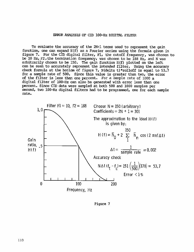
To evaluate the accuracy of the 2N+I terms used to represent the gainfunction, one can expand H(f) as a Fourier series using the formula given infigure 7. For the CID digital filter, FI, the cutoff frequency, was chosen tobe i0 Hz, F2,the termination frequency, was chosen to be 188 Hz, and N wasarbitrarily chosen to be 150. The gain function H(f) plotted on the leftcan be seen to accurately represent the intended filter. Using the .accuracycheck formula at the bottom of figure 7, N(delta t)*rolloff is equal to 53.7for a sample rate of 500. Since this value is greater than two, the errorof the filter is less than one percent. For a sample rate of i000 adigital filter of 100-Hzcanalsobegeneratedwith error less than onepercent. Since CIDdatawere sampled at both 500 and 1000 samples persecond, two 100-Hz digital filters had to be programmed, one for each samplerate.
Filter F1= 10, F2= 188 ChooseN= 150(arbitrary)1.0 Coefficients= 2N+ 1= 301
Theapproximationto the idealH(f)is given by:
150
H(f)=h0+2 _ h cos(2 ;rnfAt)Gain 1 n
ratio, . 5 \k 1H(f) At= "" 0o 002- \ samplerate
\ Accuracy check
Error < 1%I I I I i i J'_ _
0 100 200
Frequency,Hz
Figure 7
110
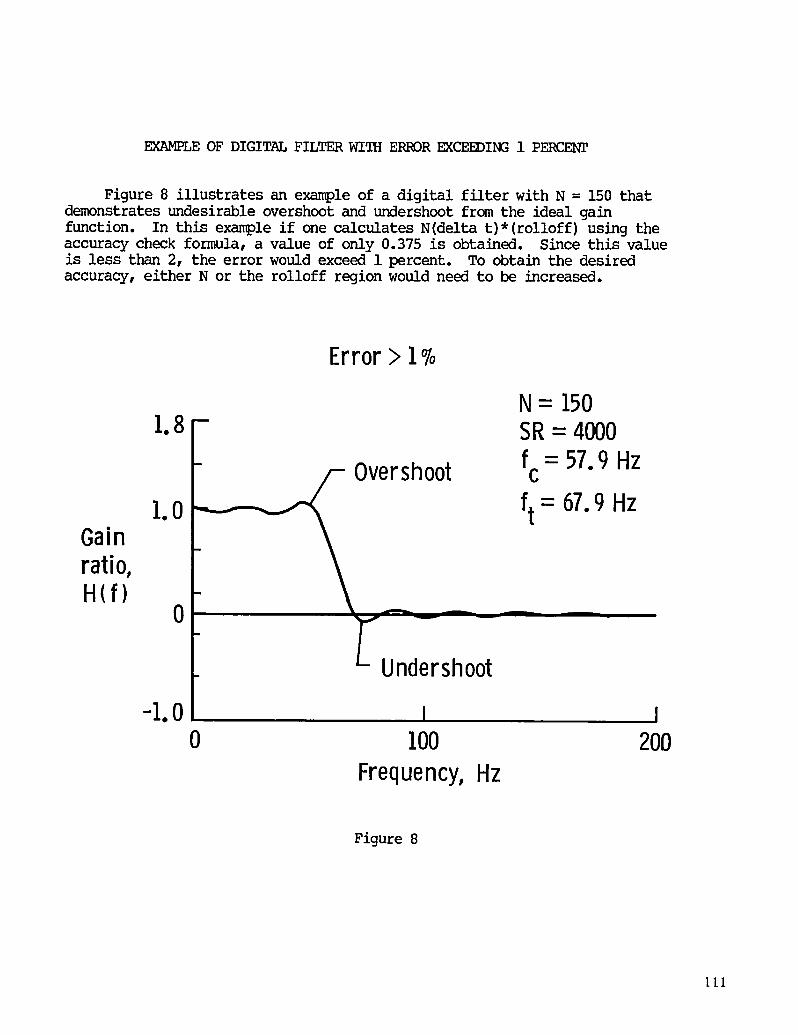
EXAMPLE OF DIGITAL FILTER WITH ERROR EXCEEDING 1 PERCENT
Figure 8 illustrates an example of a digital filter with N = 150 thatdemonstrates undesirable overshoot and undershoot from the ideal gainfunction. In this example if one calculates N(delta t)*(rolloff) using theaccuracy check formula, a value of only 0.375 is obtained. Since this valueis less than 2, the error would exceed 1 percent. To obtain the desiredaccuracy, either N or the rolloff region would need to be increased.
Error > 1%
N= 1501.8- SR= 4000
fc = 57.9 Hzr shoot
ft = 67.9HzI. 0Gainratio,H(f)
o ;n0erh 's oot
-I.0 I I0 I00 200
Frequency,Hz
Figure 8
111

PILOT FLOOR ACCELERATION NORMAL DIRECTION
The pilot floor acceleration data (normal to the floor) were sampled at500 samples per second and were taken from an accelerometer attached to the
floor at body station 228. The two plots shown in figure 9 are from channel1 for the first second after engine number one on the left wing contactedthe ground. The top plot is the raw data as recorded with no post-crashdigital filtering. The second plot shows the data after passing through the100-Hz digital filter discussed previously. The filter attenuates the highfrequencies and smoothes the digital data.
BS 228 SR= 5005-
No post filter FCH1
Acce,, 0 uU_L_J __, , _j_ul_ ,LL__bI__ ,_G -5-
-10 -
-15 t t t _ t I t i I5-
100Hz digital filterCHI
-15 i i I I t [ I t t I0 .I .2 .3 .4 .5 .6 .7 .8 .9 1.033731.00 Time, sec(9 hr 22 min II sec)
Figure 9
112

FLOOR TRACK ACCELERATION NORMAL DIRECTION
The two plots in figure i0 show the floor track acceleration for thefirst instrumented frame at body station 400. For this example, the samplerate is 1000. Again the top plot is the data with no post filter and thebottom plot is for the data passed post test through the 100-Hz digitalfilter with F1 = 10 Hz and F2 = 188 Hz. These data were taken from CIDchannel 276.
BS 400 ( Frame1) SR= 1000
18 F Nopost filter CH2768 IJ
Accel, | ...... I_ll_A.J_lX,l,l... ,.._.__.o
18 [- 100Hzdigital filter
8 _- FCH276Accel, - I __^ ._^^. _ F 10/188G -2- _ _'-_-_"-_'_-_I_I_Vl/w_'_V_'_-_-_°
-12-
-22 i i I i [ _ _ r l i0 .I .2 .3 .4 .5 .6 .7 .8 .9 1.0
33731.00 Time, sec
Figure I0
113

FLOOR ACCELERATION NORMAL FOR FRAME 2
These two acceleration traces (CID channel 120) were taken at bodystation 540. As we move back in the airplane, the acceleration levelsbecome lower and lower and the digital nature of the data is morepronounced. In figure ii the smoothing effect of the 100-Hz digital filtercan clearly be seen. In the top plot, the acceleration data are quite"stairstep looking" due to the resolution of the 8-bit digital data over the+/- 150 G range required for the normal (vertical) direction. The lowerplot, which is the same data filtered with the 100-Hz digital filter, hasall the low-frequency characteristics of the raw data without the digital"stairsteps."
BS 540 (Frame2) SR=IO002- / Nopost filter
o n |1 II111IoCH120
Accel, _JlllI]II[_Ill_l_ I_ IG -2- ?
-4 --
-6 I I I I I I I I I
2 - I00Hzdigitalfilter
0 IJU V ll/ v ^ FCH120Accel, -2 - F 10/188
G
-4 -
-6 I I I I I I I I I I
0 .i .2 .3 .4 .5 .6 .7 .8 .9 1.033731.00 Time, sec
Figure ii
114

DUMMY 14B PELVIS ACCELERATION NORMAL
The pelvis acceleration along the spineward direction for the centerdumny in the left seat in row 14 is shown in the two traces in figure 12.The sample rate is 1000 per second. Again the 100-Hz filter removes thehigh-frequency noise and cleans up the trace quite well.
2.0 F Nopostfilter CH264.5
Accel, f o
G -I.0
-2.5
-4.0 I i I i I , I i l l
2.0-100Hzdigital filter FCH264
Accel, / / _/ °G -I.0 -
-2.5
-4.0 t i l J i t i i l i0 .I .2 .3 .4 .5 .6 .7 .8 .9 1.033731.00 Time, sec
Figure 12
115

DUMMY 3E PELVIS ACCELERATION LONGI_I]DINALDIRECTION
All longitudinal accelerations measured on the aircraft and dummieswere relatively low. Since the resolution of the 8-bit system wasapproximately 1 G per count for this particular channel (an 8-bit system canhave frem 0 to 255 counts), the actual acceleration trace is only bounded bythe data. The digital filter does a reasonable job; however, it cannot makeup for the loss of resolution in this case (fig. 13).
1 F Nopost filter0 CH194
Accel,(3 -1
-2
-3 t I t J t I i t
1 _- 100Hzdigital filter FCH1940 F 10/188
AcceI,G-1 /_-_W %-/ _ I°-2
-3 I I I I I I I I I I
0 .1 .2 .3 .4 .5 .6 .7 .8 .9 1.0
33731.00 Time, sec
Figure 13
116

VERTICAL FLOOR ACCELERATION AhD INTEGRATED VELOCITY
The top plot in figure 14 is of the normal acceleration of the floor atbody station 540. The bottom plot shows the velocity curve obtained byintegrating the top acceleration plot. The dominant acceleration pulse from0.48 to 0.62 seconds in time occurs when the fuselage impacts the ground.The acceleration from 0 to 0.48 seconds is from the left wing impact.Notice that the total vertical velocity change is approximately 18 ft/s, butthat the velocity change is composed of almost 4 ft/s taken out by the wingand about 14 ft/s taken out by the fuselage. The average acceleration forthe fuselage impact can be computed from delta V of 14 ft/s divided by deltaT of 0.14 seconds which when expressed in G-units is 3.1 G's. If theacceleration from 0.48 to 0.62 seconds were a triangular pulse, then thepeak would be twice the average or 6.2 G's. For this example, twice theaverage acceleration and the peak acceleration directly from the plot arenearly the same. The average acceleration and twice the averageacceleration are useful indicators in data interpretation of crash impactseverity.
BS 540 (Frame2) Normaldirection
2- _ CIDfloorNBS _40
o m I!1 |11 IoCH120Accel, LII 11LII_1111 i/UllI
G -2 - -. _A-_ .I- Averageaccel= 3.1G'sI
-4 --
-6 t i r I If J i I I,, ; AT= 0.14
0 _-__, VCH 120
-5- T
-T
Velocity, /ft/sec-I0- AV=14.0
-15_--20 --C i i i _ -J°
0 .I .2 .3 .4 .5 .6 .7 .8 .9 1.0
33731.00 Time, sec
Figure 14
I17
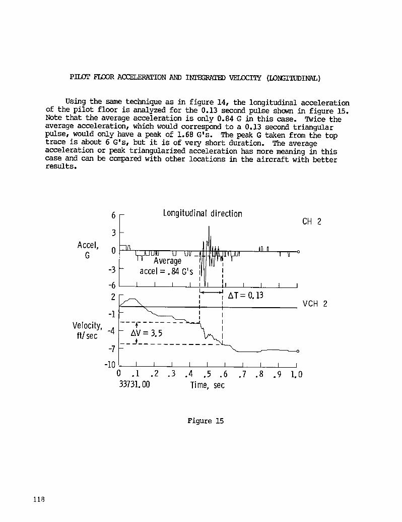
PILOT FLOOR ACCELERATION AND INTEGRATED VELOCITY (LONGI_JDINAL)
Using the same technique as in figure 14, the longitudinal accelerationof the pilot floor is analyzed for the 0.13 second pulse shown in figure 15.Note that the average acceleration is only 0.84 G in this case. Twice theaverage acceleration, which would correspond to a 0.13 second triangularpulse, would only have a peak of 1.68 G's. The peak G taken from the toptrace is about 6 G's, but it is of very short duration. The averageacceleration or peak triangularized acceleration has more meaning in thiscase and can be compared with other locations in the aircraft with betterresults.
6 Longitudinaldirection
I CH 23 I
cce,,f !Vllij l,,,G 0 r_uu_u" AverageUU-tfr'lV_,x'_' , u °
-3 accel=. 84G's
-6 i i i i ;Vj ]l i I I i2 , ,AT= 0.13
' ' VCH 2- I I-I _--_
---_Velocity, -4 - AV= 3.5ft/sec __ j_ _
-7 - \__
-10 i J j i i l l l J j0 .I .2 .3 .4 .5 .6 .7 .8 .9 1.033731.00 Time, sec
Figure 15
i18
S_C_CHANNELS-P_MARYI_A_
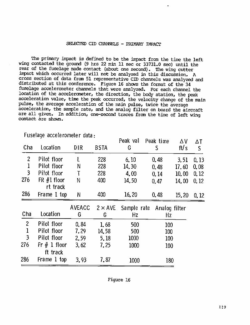
The primary impact is defined to be the impact from the time the leftwing contacted the ground (9 hrs 22 min ii sec or 33731.0 sec) until therear of the fuselage made contact (about one second). The wing cutterimpact which occurred later will not be analyzed in this discussion. Across section of data from 51 representative CID channels was analyzed anddistributed at this conference. Figure 16 shows the format of the 34fuselage accelerometer channels that were analyzed. For each channel thelocation of the accelerometer, the direction, the body station, the peakacceleration value, time the peak occurred, the velocity change of the mainpulse, the average acceleration of the main pulse, twice the averageacceleration, the sample rate, and the analog filter on board the aircraftare all given. In addition, one-second traces from the time of left wingcontact are shown.
Fuselageaccelerometer data:Peakvai Peaktime AV AT
Cha Location DIR BSTA G S ft/s S
2 Pilot floor L 228 6.10 0.48 3..51 0.131 Pilot floor N 228 14.30 0.48 17.60 0.083 Pilot floor T 228 4.00 0.14 10.00 0.12
276 FR#1 floor N 400 14o50 0.47 14.00 0.12rt track
286 Frame1 top N 400 16.20 0.48 15.20 0.12
AVEACC 2xAVE Samplerate AnalogfilterCha Location G G Hz Hz
2 Pilot floor 0.84 1.68 500 1001 Pilot floor 7.29 14.58 500 1003 Pilot floor 2.59 5.18 1000 100
276 Fr# 1 floor 3.62 7.25 1000 100ft track
286 Frame 1 top 3.93 7.87 1000 180
Figure 16
119

SELECTED CID CHANNELS - PRIMARY IMPACT
Figure 17 illustrates the format of the 14 selected channels of wingand pylon accelerometer data. Some of the velocity changes and otheranalysis are not given because of accelerometer overranging that occurredfor some channels. All of the 14 selected channels were sampled at 500samples per second and were filtered on board with 100-Hz analog filters.
Wing and pylon accelerometer data:
Sample rate: 500per secondAnalog filter: 100Hz
Peak val Peak time AV AT AVEACC 2xAVECha Location DIR BSTA G S ft/sec S G G
332 L Engine front pylon N XXXX 80.00 0.15
339 R Engine front pylon N XXXX 5.10 0.62 14.40 0.19 2.35 4.71
336 L Engine rear pylon N XXXX 162.70 0.12342 R Engine rear pylon N XXXX 28.70 0.62
184 L Wing F spar in L 806 19.10 0.11
Figure 17
120

LAP BELT LOAD CELL DATA
Figure 18 presents the lap belt load cell data for three selectedchannels. Since load cells have lower frequency response thanaccelerometers, a 50-Hz digital filter was chosen to filter the lap beltload cell data. The digital filter for load cell data attenuates more ofthe high frequencies with F1 = 6 Hz, F2 = 94 Hz, and - 3 dB attenuation for50 Hz. The loads measured in the lap belts were very low because of the lowlongitudinal accelerations in the crash.
Loadcells digitally filtered postcrash (fl = 6 Hz, f2= 94 Hz, -3dbat 50 Hz)
SampleanalogPeakval Peaktime Rate Filter
Cha Location BSTA LB S 1/S Hz
267 Dummy14Bleft belt 1220 80.00 0°98 500 60
103 Dummy14Eleft belt 1220 43.00 0.54 500 100
104 Dummy14Ert belt 1220 60.00 0.54 500 100
Figure 18
121

SUMMARY
In s_m_ary, the post processing digital filter is quite effective forremoving unwanted high frequency and noise without distorting the signal.In addition, digital filtering is effective for smoothing low-level lowresolution digital data where the digital "stairstep" phenomena arepronounced.
Integrating the acceleration data to obtain velocity traces is quiteuseful. The velocity change provides a check on the validity of theacceleration trace. (Zero offsets in acceleration must be removed before
integrating.) Average accelerations can be obtained from the velocity traceby dividing the change in velocity for an acceleration pulse by the pulseduration. One can obtain the peak of an equivalent triangular pulse bydoubling the average acceleration (fig.19).
• Digital filter effectivefor
1. Removingunwantedhigh-frequency vibrationsand noise
2. Smoothingdigital data
• Integratedacceleration(velocity) useful for
1. Obtainingvelocity changes
2. Establishingvalidity of accelerationtraces
3. Obtainingaverageaccelerations
4. Triangularizing the accelerationpulse
Figure 19
122

REFERENCES
I. Society of Automotive Engineers: Instrumentation for Impact Tests. SAEJ211a, revised 1971.
2. Graham, Ronald J. : Determination and Analysis of Numerical SmoothingWeights. NASA TR R-179, 1963.
123
Top Related