


Languages
Pages
Legal


“Difficult” problems
Marcel Maeder
Department of Chemistry
University of Newcastle
Australia

A “simple” problem
What is the pH of a 1M solution of acetic acid?
3 3K
K
CH COO H CH COOH
A H AH
What is the pH of a 1M solution of acetic acid?
4.7[ ]10
[ ][ ]
[ ] [ ] 1
AHK
A H
AH A M
2 equations and 3 unknowns: [AH], [A], [H]
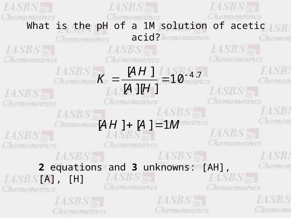
Approximation 1: Acetic acid is a weak acid, only a very small fraction dissociates and acetic acid is the only source of protons
2
[ ] 1[ ][ ] [ ]
[ ] 1
and
[ ] [ ]
1[ ]
AHK
A H H
H
H
K
AH M
A

Approximation 2: acetic acid is the only source of protons
2
2
[ ] 1 [ ] 1 [ ][ ][ ] [ ][ ] [ ]
a quadratic equation
[ ] [ ] 1 0
with s
[
ol
] [ ]
ution:
[ ]
A
AH A HK
A H A H
H
H
H
K H
H
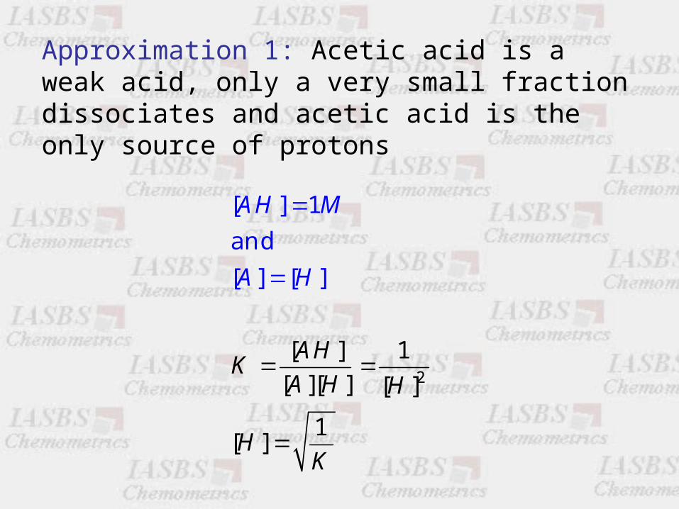
But, there are two sources of protons, acetic acid and the autodissociation of water
2
[ ] [ ] [ ] [ ] [ ]
[ ] [ ][ ]
1 [ ][ ] 1 [ ] [ ]
a cubic eqation![ ][ ] [ ][ ] ([ ] )[ ]
[ ]
w
w
w
w
AH A
H O OH
KH A OH A
H
KA H
H
KH
AH A HK
KA H A H H H
H
H
H

Activities
In reality the law of mass action really applies to activities and not concentrations.
{ }{ }{ }
where { } is the activity of the component
{ } [ ]
is the activity coeefficient of A
A
A
AHK
A H
A A
A A
More on that on Thursday

The “simple” problem of calculating the pH of a 1M acetic acid involves the solution of a cubic equation. This is possible, but the equation for that solution is very long and nobody ever uses it.
Things are much more difficult for polyprotic acids.
We need a general solution!
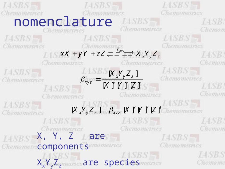
nomenclature
xyz
x y zxX yY zZ X Y Z
[ ]
[ ] [ ] [ ]x y z
xyz x y z
X Y Z
X Y Z
[ ] [ ] [ ] [ ]x y zx y z xyzX Y Z X Y Z
X, Y, Z are components
XxYyZz are species

Example: Cu + ethylene diamine, in water
NN
Components: M (Cu)
L (en)
H
Species: M
L
H
LH
LH2
ML …

Notation Species
m l h Formation constant
M (Cu2+) 1 0 0 β100=1
L (en) 0 1 0 β010=1
H (H+) 0 0 1 β001=1
LH (enH+) 0 1 1 011[ ]
[ ][ ]LH
L H
LH2 (enH22+) 0 1 2 2012 2
[ ]
[ ][ ]
LH
L H
ML (Cu(en)2+) 1 1 0 110[ ]
[ ][ ]ML
M L
ML2 (Cu(en)22+) 1 2 0 2120 2
[ ]
[ ][ ]
ML
M L
ML3 (Cu(en)32+) 1 3 0 3130 3
[ ]
[ ][ ]
ML
M L
MLH (Cu(enH)3+) 1 1 1 111[ ]
[ ][ ][ ]MLH
M L H
MLH-1 (Cu(en)(OH)+) 1 1 -1 -111-1 -1
[ ]
[ ][ ][ ]
MLH
M L H
H-1 (OH-) 0 0 -1 00-1 [ ][ ] WOH H K
3 components
11 species

2 3 -1
2 2 3 -1
2 -1
[ ] [ ] [ ] [ ] [ ] [ ] [ ]
[ ] [ ] [ ] [ ] [ ] 2[ ] 3[ ] [ ] [ ]
[ ] [ ] [ ] 2[ ] [ ] - [ ] - [ ]
tot
tot
tot
M M ML ML ML MLH MLH
L L LH LH ML ML ML MLH MLH
H H LH LH MLH MLH OH
The task is to compute all species concentrations, knowing the total concentrations of the components and the equilibrium constants
There are 11 unknowns (the species concentrations)
We need 11 equations!
3 equations for the total concentrations of the components:

111 1 1 1
111
. .
[ ]
[ ] [ ] [ ]
[ ] [ ][ ][ ]
e g
MLH
M L H
MLH M L H
8 equations for the species concentrations

2 3 -1
2 2 3 -1
2 -1
[ ] [ ] [ ] [ ] [ ] [ ] [ ]
[ ] [ ] [ ] [ ] [ ] 2[ ] 3[ ] [ ] [ ]
[ ] [ ] [ ] 2[ ] [ ] - [ ] - [ ]
tot
tot
tot
M M ML ML ML MLH MLH
L L LH LH ML ML ML MLH MLH
H H LH LH MLH MLH OH
[ ] [ ] [ ] [ ]
[ ] [ ] [ ] [ ]
[ ] [ ] [ ] [ ]
m l htot mlh
m l htot mlh
m l htot mlh
M m M L H
L l M L H
H h M L H
Generalised equations:
c_spec =beta.*prod(repmat(c',1,nspec).^Model,1); %species conc
c_tot_calc=sum(Model.*repmat(c_spec,ncomp,1),2)'; %comp ctot calc
Allow very compact MATLAB code:

How can we write a MATLAB program that can resolve these systems of many unknowns with many
equations and that can deal with any model?
The Newton-Raphson algorithm

The Taylor series expansion
2 ( )1 1 1( ) ( ) '( ) ''( ) ... ( ) ...
1! 2! !n nf x x f x f x x f x x f x x
n
2 ( )1 1 1( ) ( ) '( ) ''( ) ... ( ) ...
1! 2! !n n
nf x x f x f x x f x x f x x
( ) ( ) '( )f x x f x f x x
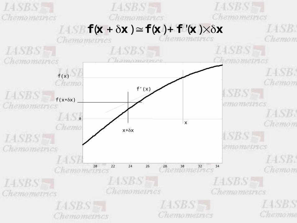
( ) ( ) '( )f x x f x f x x
20 22 24 26 28 30 32 34
0x
f(x)
f’(x)
x+x
f(x+x)

The function to minimise is:
The difference between the known total concentrations and the calculated values:
t[ ] [ ] [ ] [ ]
( ) [ ] [ ] [ ] [ ]
[ ] [ ] [ ] [ ]
x y ztot xyz
x y ztot xyz
x y ztot xyz
X x X Y Z
Y y X Y Z
Z z X Y Z
d d c
[ ] [ ] [ ]X Y Zc

( )( + ) = ( ) +
d c
d c c d c cc
= +
d(c+c) d(c) c ( )d cc
= +
d(c+c) d(c) c ( )d cc
1( )
= ( )
d cc d c
c

2 31
1 1 1
2 31
2 2 2
2 31
3 3 3
d ddc c c
d ddc c c
d ddc c c
dJ
c
The Jacobian J

1
1
2 3
1 1
2 31
2 2 2
2 31
3 3 3
d dc c
d ddc c
dc
c
d ddc c c
dJ
c
2 1
2
2
[ ] [ ] [ ] [ ]
[ ] [ ]
[ ] [ ] [ ]
[ ]
[ ] [ ] [ ]
[ ] [ ] [ ]
[ ]
[ ]
[ ]
x y ztot xyzX
x y zxyz
x y zxyz
x y zxyz
x y z
X x X Y ZdX X
x X Y Z
X
x X Y Z
x X Y Z
X
x X Y Z
X

2
2
2 [ ] [ ]
[ ] [ ]
[ ] [ ] [ ]( )[ ] [ ] [
[ ]
[ ]
]
[ ] [ ] [ ]
[ ] [ ] [ ]
x y z x y z
x y z x y z x y z
x y z
x y z
x y z x y z
xy X Y Z xz X Y Z
X X
xy X Y Z y X Y Z yz X Y Z
Y Y Y
xz X Y Z yz X Y Z z X Y Z
Z Z
Y Z
X
Z
x X
d cJ
c

Compare actual total conc. with computed ones
e.g.
Guess initial concentrations for the free component concentrations
[X], [Y], [Z]
Calculate the concentrations of all species
e.g. XxYyZz=xyz [X]x[Y]y[Z]z
Calculate J acobian
Calculate shift vector and add to component concentrations
Difference
>0
0Exit
Calculate the total concentration of the components
e.g. _[ ] [ ] [ ] [ ]x y ztot calc xyzX x X Y Z
_[ ] [ ]x tot tot calcd X X


• Kinetics at non-constant temperature
• Kinetics and equilibria, taking into account changes in ionic strength
• Kinetics at non-constant pH

Why?
• In traditional measurements temperature, ionic strength, pH are kept constant using buffers, excess inert salt, thermostatting
• All these external means are only required to simplify the computations. If it is possible to take changes in these parameters into account, buffers etc are no more required
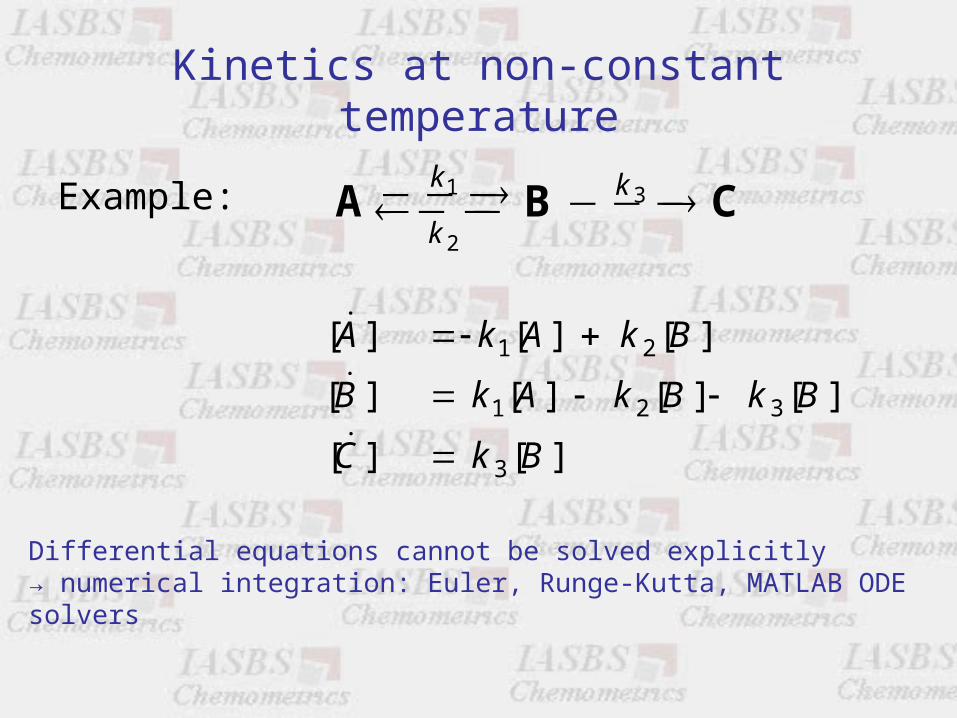
Kinetics at non-constant temperature
Example: 1 3
2
k k
k A B C
1 2
1 2 3
3
[ ] [ ] [ ]
[ ] [ ] [ ] [ ]
[ ] [ ]
A k A k B
B k A k B k B
C k B
Differential equations cannot be solved explicitly → numerical integration: Euler, Runge-Kutta, MATLAB ODE solvers

This function computes the derivatives of the concentrations vs. time (c_dot) at time t for a given set of concentrations c.
The rest is done by the ODE-solver
1 2
1 2 3
3
[ ] [ ] [ ]
[ ] [ ] [ ] [ ]
[ ] [ ]
A k A k B
B k A k B k B
C k B
Translation into MATLAB language, the function ode_AeqBtoC.m is used by the MATLAB ode-solvers
function c_dot=ode_AeqBtoC(t,c,flag,k)
% A <-> B
% B --> C
c_dot(1,1)=-k(1)*c(1)+k(2)*c(2); % A_dot
c_dot(2,1)= k(1)*c(1)-k(2)*c(2)-k(3)*c(2); % B_dot
c_dot(3,1)= k(3)*c(2); % C_dot
ode_AeqBtoC.m

0 50 100 150 200 250 3000
0.1
0.2
0.3
0.4
0.5
0.6
0.7
0.8
0.9
1
time
conc
.
Fast first reaction and slow second reaction
Difficult to observe both in one measurement
c0=[1;0;0]; % initial conc of A, Cat, B and C
k=[.2;.1;.01]; % rate constants k1 and k2
times=[0:1:300]';
[times,C] = ode45('ode_AeqBtoC',times,c0,[],k); % call ode-solver
figure(1); plot(times,C) % plotting C vs t
xlabel('time');ylabel('conc.');
AeqBtoC.m
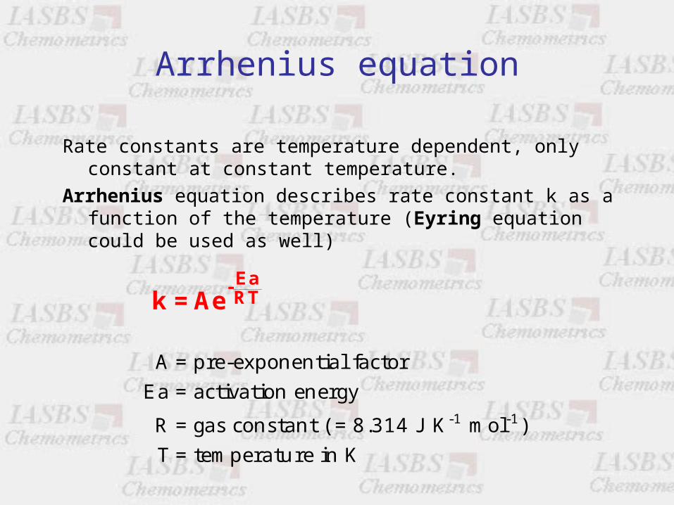
Arrhenius equation
Rate constants are temperature dependent, only constant at constant temperature.
Arrhenius equation describes rate constant k as a function of the temperature (Eyring equation could be used as well)
-1 -1
A = pre-exponential factor
Ea = activation energy
R = gas constant ( = 8.314 J K mol )
T = temperature in K
Ea-RTk =Ae
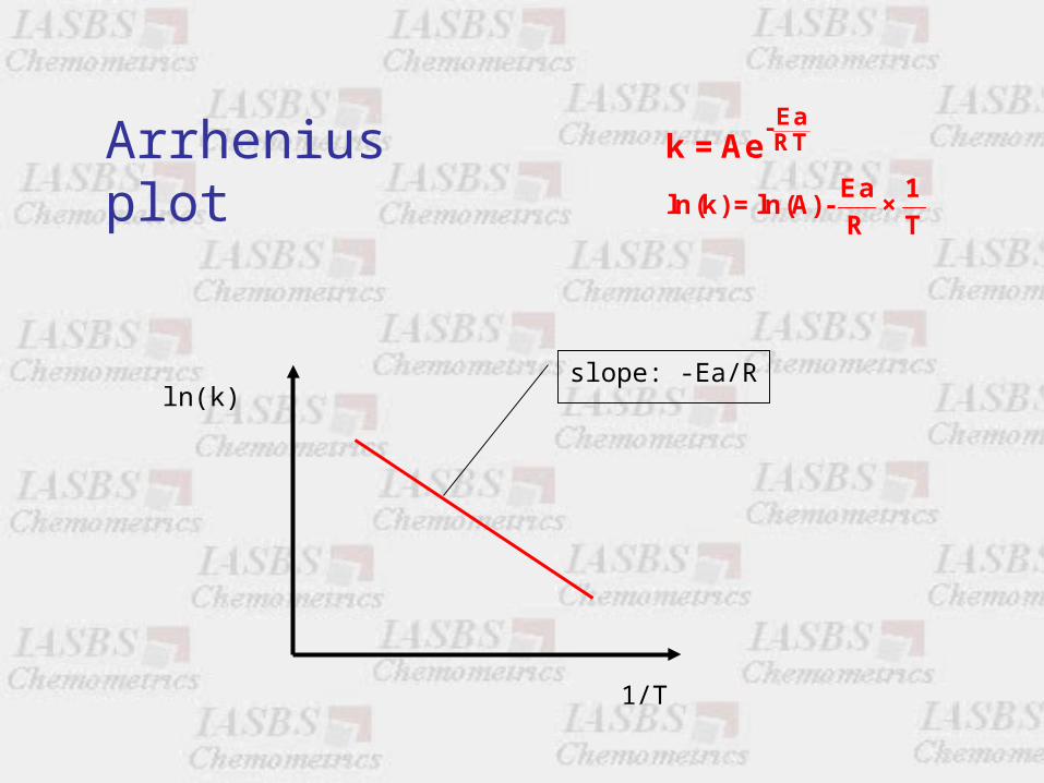
Arrhenius plotEa-RT
Ea 1ln(k)=ln(A)- ×
R T
k =Ae
ln(k)
1/T
slope: -Ea/R
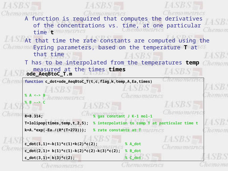
A function is required that computes the derivatives of the concentrations vs. time, at one particular time t
At that time the rate constants are computed using the Eyring parameters, based on the temperature T at that time
T has to be interpolated from the temperatures temp measured at the times times
function c_dot=ode_AeqBtoC_T(t,c,flag,k,temp,A,Ea,times)
% A <-> B
% B --> C
R=8.314; % gas constant J K-1 mol-1
T=lolipop(times,temp,t,2,5); % interpolation to comp T at particular time t
k=A.*exp(-Ea./(R*(T+273))); % rate constants at T
c_dot(1,1)=-k(1)*c(1)+k(2)*c(2); % A_dot
c_dot(2,1)= k(1)*c(1)-k(2)*c(2)-k(3)*c(2); % B_dot
c_dot(3,1)= k(3)*c(2); % C_dot
ode_AeqBtoC_T.m

A =[12.13 1.77 36.79]; % pre-exp factor for each rate constant
Ea=[1e4 7e3 2e4]; % activation energies
temp=20+0.2*times; % temperatures at measurement times
[times,C] = ode45('ode_AeqBtoC_T',times,c0,[],k,temp,A,Ea,times); % ode-solver
figure(2); plot(times,C) % plotting C vs t
xlabel('time');ylabel('conc.');
AeqBtoC.m … contiuned

0 50 100 150 200 250 3000
0.1
0.2
0.3
0.4
0.5
0.6
0.7
0.8
0.9
1
time
conc
.
0 50 100 150 200 250 3000
0.1
0.2
0.3
0.4
0.5
0.6
0.7
0.8
0.9
1
time
conc
.at 20°C at 20-80°C
Similar to temperature program in GC or non-isocratic mobile phase in HPLC

Modeling - Fitting
• The core of the fitting algorithm is the modeling of the measurement and in most cases this is the computation of the matrix C
• This is exactly what we have done so far for non-isothermal kinetics• The parameters used to model the concentration profiles can, at least
potentially, also be fitted to appropriate data• In this case non-isothermal measurements allows the determination
of the activation parameters of all rate constants• Much more convenient than classical method of repeating the
measurement at different temperatures with subsequent Arrhenius analysis
Newton-Gauss Algorithmii) Calculation the residuals and ssq according to model and estimated parameters
Calculation of residual matrix
R = A – C (C\A)
400 420 440 460 480 500 520 540 560 580 600-0.1
-0.08
-0.06
-0.04
-0.02
0
0.02
0.04
0.06
Wavelength (nm)
Abs
orba
nce
400 420 440 460 480 500 520 540 560 580 600-0.2
0
0.2
0.4
0.6
0.8
1
1.2
Wavelength (nm)
Abs
orba
nce
400 420 440 460 480 500 520 540 560 580 6000
0.2
0.4
0.6
0.8
1
1.2
1.4Simulated Spectra
Wavelength (nm)
Abs
orba
nce
--- =
ssq = SS r2I,j = 1.66

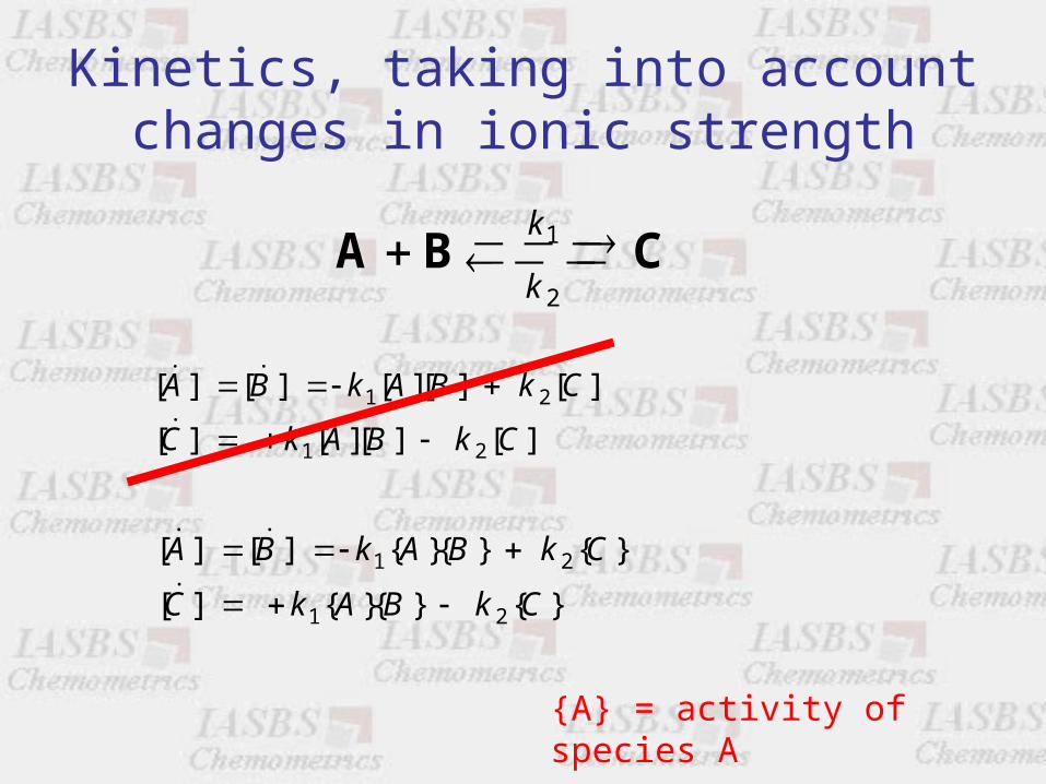
Kinetics, taking into account changes in ionic strength
1
2
k
k A B C
1 2
1 2
[ ] [ ] [ ][ ] [ ]
[ ] [ ][ ] [ ]
A B k A B k C
C k A B k C
1 2
1 2
[ ] [ ] { }{ } { }
[ ] { }{ } { }
A B k A B k C
C k A B k C
{A} = activity of species A
Kinetics, taking into account changes in ionic strength
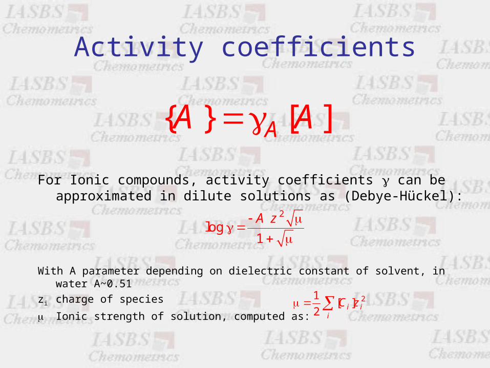
Activity coefficients
For Ionic compounds, activity coefficients can be approximated in dilute solutions as (Debye-Hückel):
With A parameter depending on dielectric constant of solvent, in water A~0.51
zi charge of species
Ionic strength of solution, computed as:
{ } [ ]AA A
2 log
1
A z
21[ ]
2 i ii
C z

1
2
k
k A B C
1 2
1 2
[ ] [ ] { }{ } { }
[ ] { }{ } { }
A B k A B k C
C k A B k C
2 log ...
1A
AA z
2 2 21([ ] [ ] [ ] )
2 A B CA z B z C z
As the concentrations change during the reaction, the ionic strength and all activity coefficients change as well.

Example
1
2
2 34 4( )
k
kSO Fe Fe SO
1M Na2SO41M Fe(ClO4)3 1M Na+
0.5 M SO42-
0.5 M Fe3+
1.5 M ClO4-
+ →

1M Na+
0.5 M SO42-
0.5 M Fe3+
1.5 M ClO4-
2 2 3 24 4
2 2
1([ ] [ ]2 [ ]3 [ ])
21
(1 0.5 2 0.5 3 1.5)21
(1 2 4.5 1.5)24.5
Na SO Fe ClO
2
24
2
3
0.5 1 4.5
1 4.5
0.5 2 4.5
1 4.5
0.5 3 4.541 4.5
10 0.46
10 0.044
10 8.7 10
Na
SO
Fe
Note: Debye-Hückel equation not valid at such high concentrations !
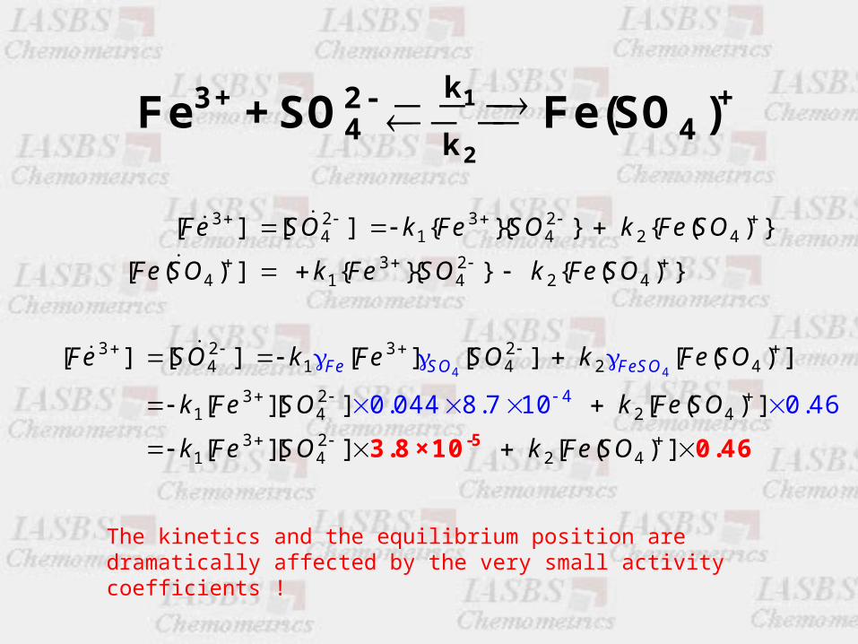
1
2
k3+ 2- +4 4k
Fe +SO Fe(SO )
3 2 3 24 1 4 2 4
3 24 1 4 2 4
[ ] [ ] { }{ } { ( ) }
[ ( ) ] { }{ } { ( ) }
Fe SO k Fe SO k Fe SO
Fe SO k Fe SO k Fe SO
4 4
3 2 3 24 1 4 2 4
3 21 4 2 4
3 21 4 2 4
4
[ ] [ ] [ ] [ ] [ ( ) ]
[ ][ ] 0.044 8.7 10 0.4 [ ( ) ]
[ ][ ] [ ( ) ]
6
Fe SO FeSOFe SO k Fe SO k Fe SO
k Fe SO k Fe SO
k Fe SO k Fe SO
-53.8×10 0.46
The kinetics and the equilibrium position are dramatically affected by the very small activity coefficients !
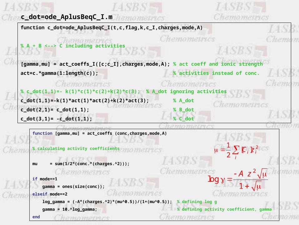
function c_dot=ode_AplusBeqC_I(t,c,flag,k,c_I,charges,mode,A)
% A + B <--> C including activities
[gamma,mu] = act_coeffs_I([c;c_I],charges,mode,A); % act coeff and ionic strength
act=c.*gamma(1:length(c)); % activities instead of conc.
% c_dot(1,1)=- k(1)*c(1)*c(2)+k(2)*c(3); % A_dot ignoring activities
c_dot(1,1)=-k(1)*act(1)*act(2)+k(2)*act(3); % A_dot
c_dot(2,1)= c_dot(1,1); % B_dot
c_dot(3,1)= -c_dot(1,1); % C_dot
c_dot=ode_AplusBeqC_I.m
function [gamma,mu] = act_coeffs (conc,charges,mode,A)
% calculating activity coefficients
mu = sum(1/2*(conc.*(charges.^2)));
if mode==1
gamma = ones(size(conc));
elseif mode==2
log_gamma = (-A*(charges.^2)*(mu^0.5))/(1+(mu^0.5)); % defining log g
gamma = 10.^log_gamma; % defining activity coefficient, gamma
end
2 log
1
A z
21[ ]
2 i ii
C z
0 50 100 150 200 250 3000
0.001
0.002
0.003
0.004
0.005
0.006
0.007
0.008
0.009
0.01
time
conc
.
0 50 100 150 200 250 3000
0.001
0.002
0.003
0.004
0.005
0.006
0.007
0.008
0.009
0.01
time
conc
.
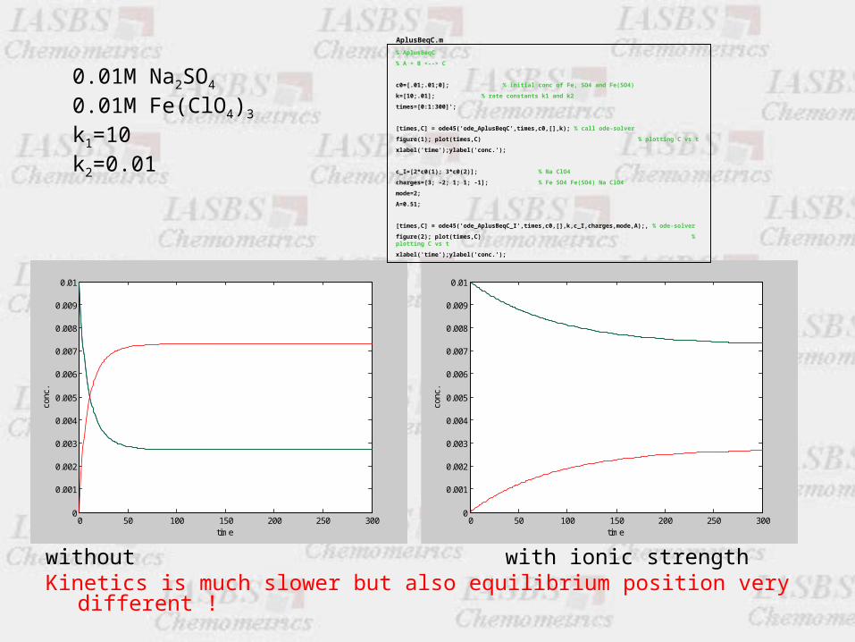
0.01M Na2SO4
0.01M Fe(ClO4)3
k1=10k2=0.01
without with ionic strengthKinetics is much slower but also equilibrium position very different !
% AplusBeqC
% A + B <--> C
c0=[.01;.01;0]; % initial conc of Fe, SO4 and Fe(SO4)
k=[10;.01]; % rate constants k1 and k2
times=[0:1:300]';
[times,C] = ode45('ode_AplusBeqC',times,c0,[],k); % call ode-solver
figure(1); plot(times,C) % plotting C vs t
xlabel('time');ylabel('conc.');
c_I=[2*c0(1); 3*c0(2)]; % Na ClO4
charges=[3; -2; 1; 1; -1]; % Fe SO4 Fe(SO4) Na ClO4
mode=2;
A=0.51;
[times,C] = ode45('ode_AplusBeqC_I',times,c0,[],k,c_I,charges,mode,A);, % ode-solver
figure(2); plot(times,C) % plotting C vs t
xlabel('time');ylabel('conc.');
AplusBeqC.m
Equilibrium calculations are more complex:
In kinetics, using an ODE solver, the only requirement is to compute the derivatives of the concentrations vs. time for a given set of concentrations. Thus, it is possible to calculate the activity coefficients at that moment and incorporate into the derivatives.
In equilibria, the activity coefficients depend on the concentrations and the concentrations depend on the activities. An internal iterative process is required.

Titration of phosphoric acid:1
2
3
3 24 4
34 2 4
34 3 4
2
3
PO H HPO
PO H H PO
PO H H PO
24
24
2 24 4
1 3 34 4
{ } [ ]
{ }{ } [ ][ ]HPO
HPO H
HPO HPO
PO H PO H
3 2 2 24 4
1([ ] [ ] 3 +[ ] 2 + )
2H PO HPO
2 4
0.5 1
110H H PO

Iterative approach:
Guess -valuesCalculate concentrationsCalculate new -values

Newton-Raphson algorithm
• The core is the computation of the difference d between actual and computed total concentrations c, and
• The derivatives of these with respect to the total concentrations
dc
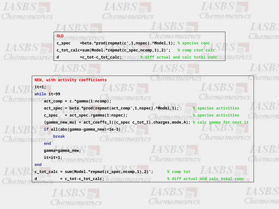
OLD
c_spec =beta.*prod(repmat(c',1,nspec).^Model,1); % species conc
c_tot_calc=sum(Model.*repmat(c_spec,ncomp,1),2)'; % comp ctot calc
d =c_tot-c_tot_calc; % diff actual and calc total conc
NEW, with activity coefficients
it=1;
while it<99
act_comp = c.*gamma(1:ncomp);
act_spec = beta.*prod(repmat(act_comp',1,nspec).^Model,1); % species activities
c_spec = act_spec./gamma(1:nspec); % species activities
[gamma_new,mu] = act_coeffs_I([c_spec c_tot_I],charges,mode,A); % calc gamma for next it
if all(abs(gamma-gamma_new)<1e-3)
break
end
gamma=gamma_new;
it=it+1;
end
c_tot_calc = sum(Model.*repmat(c_spec,ncomp,1),2)'; % comp tot
d = c_tot-c_tot_calc; % diff actual and calc total conc

3 22 4 2 4{ } { }{ } H PO PO H
34
3 34 4{ } [ ]
{ } [ ]
PO
H
PO PO
H H
2 42 4 2 4[ ] { }/
H POH PO H PO
22 4
1([ ] 1 )
2H PO
2 4
0.5 1
110 H PO
constant ?no
yes
guess
act_comp = c.*gamma(1:ncomp);
act_spec = beta.*prod(repmat(act_comp',1,nspec).^Model,1);
c_spec = act_spec./gamma(1:nspec);
[gamma_new,mu]= act_coeffs_I([c_spec c_tot_I],charges,mode,A);
if all(abs(gamma-gamma_new)<1e-3)

0 0.005 0.01 0.015 0.02 0.025 0.03 0.0350
2
4
6
8
10
12
vol. added (L)
pH
2 3 4 5 6 7 8 9 10 11 120
0.005
0.01
0.015
0.02
0.025
10.1 10.2 10.3 10.4 10.5 10.6 10.7 10.8 10.9 11
0
1
2
3
4
5
6
7
8
9
x 10-3
10 ml of 0.03M H3PO4 (pK 11,7,3)
titrated with 35ml of 0.01M NaOH
HPO42- PO4
3-
[HPO42-] [PO4
3-] at pH = pK
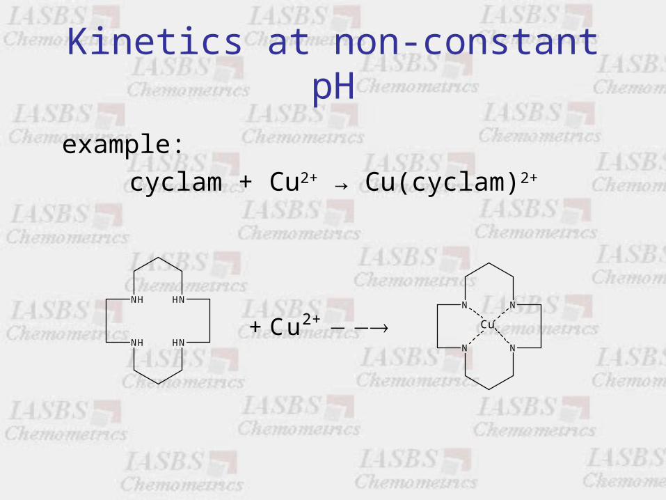
Kinetics at non-constant pH
example:cyclam + Cu2+ → Cu(cyclam)2+
N N
NN
Cu
NH HN
HNNH
2++ Cu

1
2
3
4
K+ +
K+ + 2+2
K2+ + 3+2 3
K3+ + 4+3 4
L + H LH
LH + H LH
LH + H LH
LH + H LH
NH HN
HNNH
Cyclam has 4 secondary amines that are protonated depending on the pH of the solution
4 protonation equilibria and 4 protonation constants define all concentrations [L], [LH+], …

L
L
LH
H
L
3
H
2
LH
4
k2+ 2+ 2+ +2
k2+ 3+ 2+ +3
k2+ 2+
k2+ + 2+ +
k2+ 4+ 2+4
Cu + L ML only at very high pH
Cu + LH ML + H only at very hig
Cu
h pH
Cu + LH ML
+ LH ML +2H
Cu + LH ML +3H
++4H only at very low pH
N N
NN
Cu
2+LH2k
2++ Cu
Each of the five differently protonated forms of cyclam reacts with Cu2+ with a particular rate constant.
E.g.
NH2+ HN
+H2NNH
LH2
LH3
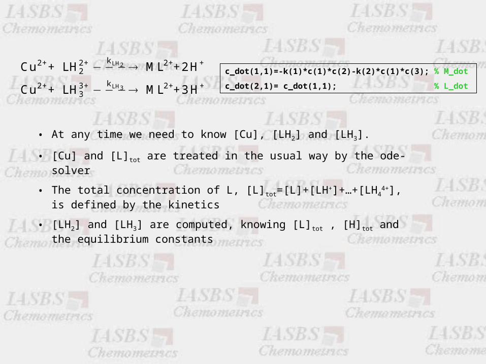
k2+ 2+ 2+ +2
k2+ 3+ 2+ +3
Cu + LH ML +2H
Cu + LH ML +3H
c_dot(1,1)=-k(1)*c(1)*c(2)-k(2)*c(1)*c(3); % M_dot
c_dot(2,1)= c_dot(1,1); % L_dot
• At any time we need to know [Cu], [LH2] and [LH3].
• [Cu] and [L]tot are treated in the usual way by the ode-solver
• The total concentration of L, [L]tot=[L]+[LH+]+…+[LH44+], is
defined by the kinetics
• [LH2] and [LH3] are computed, knowing [L]tot , [H]tot and the equilibrium constants

function c_dot=ode_CuCyclam (t,c,flag,k,c_0,equil_model,beta)
% kinetics
% M + LH > ML + H
% M + LH2> ML + 2H
% equilibria
% L,LH,LH2,LH3,LH4,OH
% c =[M Ltot]
% c_0 =[M_0, Ltot_0, H_tot]
c_tot=[c(2),c_0(3)]; %[Ltot,Htot], the conc of free protons is constant
c_comp_guess = [1e-10 1e-10]; % initial guess for [L],[H]
L_eq=NewtonRaphson(equil_model, beta, c_tot, c_comp_guess,i); % [L] [H] [LH] [LH2] [LH3] [LH4] [OH]
c=[c(1) L_eq(3) L_eq(4)]; % [M], [LH], [LH2]
c_dot(1,1)=-k(1)*c(1)*c(2)-k(2)*c(1)*c(3); % M_dot
c_dot(2,1)= c_dot(1,1); % L_dot
ode_CuCyclam.m

%Main_CuCyclam
c_0=[0.004 0.005 0.015]; % initial concs Ltot,M,H
k=[1050000 0.135]; % rate constants
times=[1:100:10000]';
spec_names = {'L' 'H' 'LH' 'LH2' 'LH3' 'LH4' 'OH'};
equil_model = [ 1 0 1 1 1 1 0; ... % L
0 1 1 2 3 4 -1] ; % H
log_beta = [ 0 0 11.59 22.21 23.82 26.24 -14];
beta =10.^log_beta;
[times,C] = ode45('ode_CuCyclam',times,c_0(1:2),[],k,c_0,equil_model,beta); % C=(Ltot M)
c_comp_guess = [1e-10 1e-10]; % computing L_eq from Ltot and H
for i=1:length(times)
L_eq(i,:)=NewtonRaphson(equil_model, beta, [C(i,1) c_0(3)], c_comp_guess,i); % [L] [H] [LH] [LH2] [LH3] [LH4] [OH]
c_comp_guess = L_eq(i,1:2); % using calc conc as estimates for next iteration
end
plot(times,C,'.',times,L_eq);
Main_CuCyclam.m

0 1000 2000 3000 4000 5000 6000 7000 8000 9000 100000
0.002
0.004
0.006
0.008
0.01
0.012
0.014
[M] [L]tot
[H][LH2]
[LH3]
[LH4]
c_0=[0.004 0.005 0.015]; % initial concs Ltot,M,H
Top Related