


Languages
Pages
Legal


CHAPTER 7
Differentiation
1. The Derivative at a Point
DEFINITION 7.1. Let f be a function defined on a neighborhood of x0. f isdifferentiable at x0, if the following limit exists:
f0(x0) = lim
h!0
f (x0 +h)° f (x0)h
.
Define D( f ) = {x : f0(x) exists}.
The standard notations for the derivative will be used; e.g., f0(x), d f (x)
d x, D f (x),
etc.
An equivalent way of stating this definition is to note that if x0 2 D( f ), then
f0(x0) = lim
x!x0
f (x)° f (x0)x °x0
.
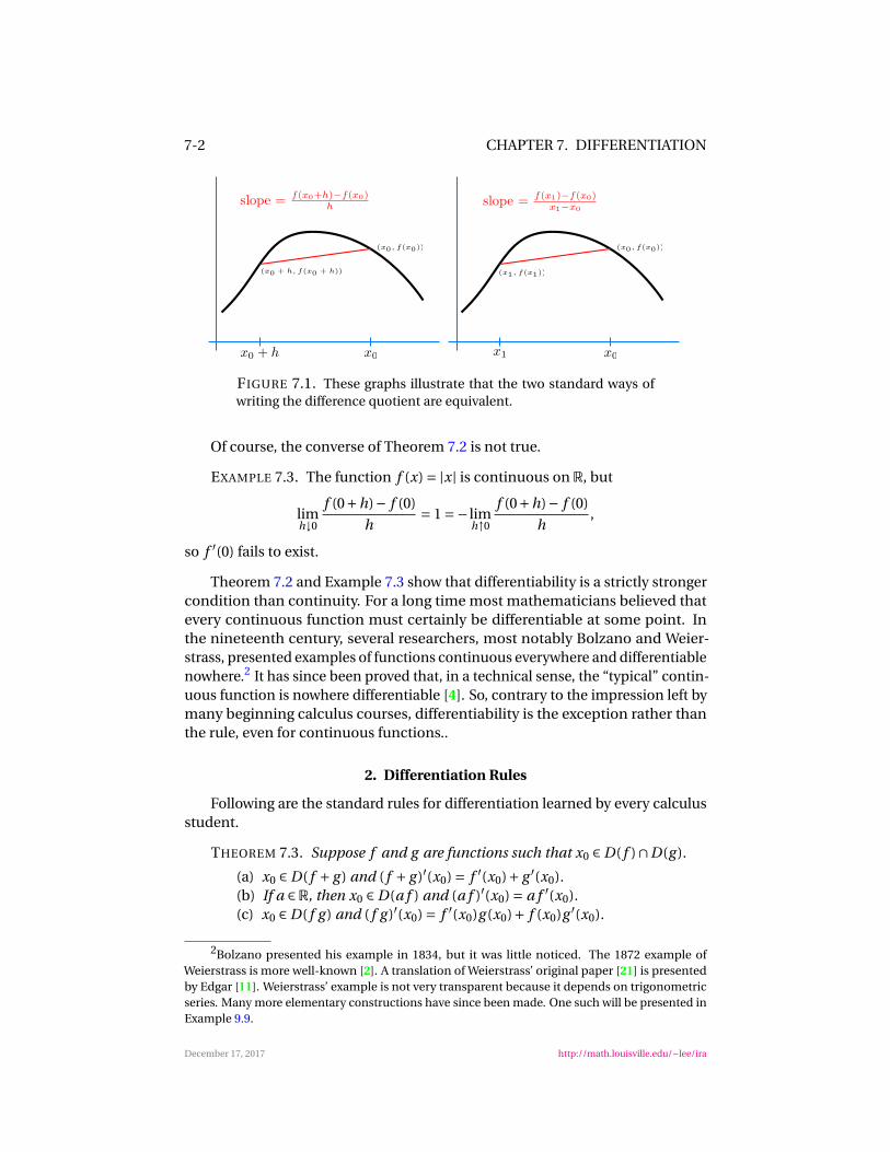
(See Figure 1.)This can be interpreted in the standard way as the limiting slope of the secant
line as the points of intersection approach each other.
EXAMPLE 7.1. If f (x) = c for all x and some c 2R, then
limh!0
f (x0 +h)° f (x0)h
= limh!0
c ° c
h= 0.
So, f0(x) = 0 everywhere.
EXAMPLE 7.2. If f (x) = x, then
limh!0
f (x0 +h)° f (x0)h
= limh!0
x0 +h °x0
h= lim
h!0
h
h= 1.
So, f0(x) = 1 everywhere.
THEOREM 7.2. For any function f , D( f ) ΩC ( f ).
PROOF. Suppose x0 2 D( f ). Then
limx!x0
°f (x)° f (x0)
¢= lim
x!x0
f (x)° f (x0)x °x0
(x °x0)
= f0(x0) 0 = 0.
This shows limx!x0 f (x) = f (x0), and x0 2C ( f ). ⇤1December 17, 2017 ©Lee Larson ([email protected])
7-1
7-2 CHAPTER 7. DIFFERENTIATION
FIGURE 7.1. These graphs illustrate that the two standard ways ofwriting the difference quotient are equivalent.
Of course, the converse of Theorem 7.2 is not true.
EXAMPLE 7.3. The function f (x) = |x| is continuous on R, but
limh#0
f (0+h)° f (0)h
= 1 =° limh"0
f (0+h)° f (0)h
,
so f0(0) fails to exist.
Theorem 7.2 and Example 7.3 show that differentiability is a strictly strongercondition than continuity. For a long time most mathematicians believed thatevery continuous function must certainly be differentiable at some point. Inthe nineteenth century, several researchers, most notably Bolzano and Weier-strass, presented examples of functions continuous everywhere and differentiablenowhere.2 It has since been proved that, in a technical sense, the “typical” contin-uous function is nowhere differentiable [4]. So, contrary to the impression left bymany beginning calculus courses, differentiability is the exception rather thanthe rule, even for continuous functions..
2. Differentiation Rules
Following are the standard rules for differentiation learned by every calculusstudent.
THEOREM 7.3. Suppose f and g are functions such that x0 2 D( f )\D(g ).
(a) x0 2 D( f + g ) and ( f + g )0(x0) = f0(x0)+ g
0(x0).
(b) If a 2R, then x0 2 D(a f ) and (a f )0(x0) = a f0(x0).
(c) x0 2 D( f g ) and ( f g )0(x0) = f0(x0)g (x0)+ f (x0)g
0(x0).
2Bolzano presented his example in 1834, but it was little noticed. The 1872 example ofWeierstrass is more well-known [2]. A translation of Weierstrass’ original paper [21] is presentedby Edgar [11]. Weierstrass’ example is not very transparent because it depends on trigonometricseries. Many more elementary constructions have since been made. One such will be presented inExample 9.9.
December 17, 2017 http://math.louisville.edu/ªlee/ira
2. DIFFERENTIATION RULES 7-3
(d) If g (x0) 6= 0, then x0 2 D( f /g ) and
µf
g
∂0(x0) = f
0(x0)g (x0)° f (x0)g0(x0)
(g (x0))2 .
PROOF. (a)
limh!0
( f + g )(x0 +h)° ( f + g )(x0)h
= limh!0
f (x0 +h)+ g (x0 +h)° f (x0)° g (x0)h
= limh!0
µf (x0 +h)° f (x0)
h+ g (x0 +h)° g (x0)
h
∂= f
0(x0)+ g0(x0)
(b)
limh!0
(a f )(x0 +h)° (a f )(x0)h
= a limh!0
f (x0 +h)° f (x0)h
= a f0(x0)
(c)
limh!0
( f g )(x0 +h)° ( f g )(x0)h
= limh!0
f (x0 +h)g (x0 +h)° f (x0)g (x0)h
Now, “slip a 0” into the numerator and factor the fraction.
= limh!0
f (x0 +h)g (x0 +h)° f (x0)g (x0 +h)+ f (x0)g (x0 +h)° f (x0)g (x0)h
= limh!0
µf (x0 +h)° f (x0)
hg (x0 +h)+ f (x0)
g (x0 +h)° g (x0)h
∂
Finally, use the definition of the derivative and the continuity of f and g at x0.
= f0(x0)g (x0)+ f (x0)g
0(x0)
(d) It will be proved that if g (x0) 6= 0, then (1/g )0(x0) = °g0(x0)/(g (x0))2. This
statement, combined with (c), yields (d).
limh!0
(1/g )(x0 +h)° (1/g )(x0)h
= limh!0
1g (x0 +h)
° 1g (x0)
h
= limh!0
g (x0)° g (x0 +h)h
1g (x0 +h)g (x0)
=° g0(x0)
(g (x0)2
Plug this into (c) to seeµ
f
g
∂0(x0) =
µf
1g
∂0(x0)
= f0(x0)
1g (x0)
+ f (x0)°g
0(x0)(g (x0))2
= f0(x0)g (x0)° f (x0)g
0(x0)(g (x0))2 .
⇤
December 17, 2017 http://math.louisville.edu/ªlee/ira
7-4 CHAPTER 7. DIFFERENTIATION
Combining Examples 7.1 and 7.2 with Theorem 7.3, the following theorem iseasy to prove.
COROLLARY 7.4. A rational function is differentiable at every point of its do-
main.
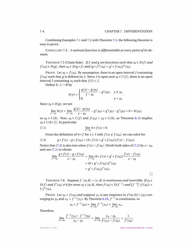
THEOREM 7.5 (Chain Rule). If f and g are functions such that x0 2 D( f ) and
f (x0) 2 D(g ), then x0 2 D(g ± f ) and (g ± f )0(x0) = g0 ± f (x0) f
0(x0).
PROOF. Let y0 = f (x0). By assumption, there is an open interval J containingf (x0) such that g is defined on J . Since J is open and x0 2C ( f ), there is an openinterval I containing x0 such that f (I ) Ω J .
Define h : J !R by
h(y) =
8<
:
g (y)° g (y0)y ° y0
° g0(y0), y 6= y0
0, y = y0
.
Since y0 2 D(g ), we see
limy!y0
h(y) = limy!y0
g (y)° g (y0)y ° y0
° g0(y0) = g
0(y0)° g0(y0) = 0 = h(y0),
so y0 2 C (h). Now, x0 2 C ( f ) and f (x0) = y0 2 C (h), so Theorem 6.15 impliesx0 2C (h ± f ). In particular
(7.1) limx!x0
h ± f (x) = 0.
From the definition of h ± f for x 2 I with f (x) 6= f (x0), we can solve for
(7.2) g ± f (x)° g ± f (x0) = (h ± f (x)+ g0 ± f (x0))( f (x)° f (x0)).
Notice that (7.2) is also true when f (x) = f (x0). Divide both sides of (7.2) by x°x0,and use (7.1) to obtain
limx!x0
g ± f (x)° g ± f (x0)x °x0
= limx!x0
(h ± f (x)+ g0 ± f (x0))
f (x)° f (x0)x °x0
= (0+ g0 ± f (x0)) f
0(x0)
= g0 ± f (x0) f
0(x0).
⇤THEOREM 7.6. Suppose f : [a,b] ! [c,d ] is continuous and invertible. If x0 2
D( f ) and f0(x0) 6= 0 for some x0 2 (a,b), then f (x0) 2 D( f
°1) and°
f°1¢0 ( f (x0)) =
1/ f0(x0).
PROOF. Let y0 = f (x0) and suppose yn is any sequence in f ([a,b]) \ {y0} con-verging to y0 and xn = f
°1(yn). By Theorem 6.24, f°1 is continuous, so
x0 = f°1(y0) = lim
n!1f°1(yn) = lim
n!1xn .
Therefore,
limn!1
f°1(yn)° f
°1(y0)yn ° y0
= limn!1
xn °x0
f (xn)° f (x0)= 1
f 0(x0).
December 17, 2017 http://math.louisville.edu/ªlee/ira
3. DERIVATIVES AND EXTREME POINTS 7-5
⇤EXAMPLE 7.4. It follows easily from Theorem 7.3 that f (x) = x
3 is differ-entiable everywhere with f
0(x) = 3x2. Define g (x) = 3
px. Then g (x) = f
°1(x).Suppose g (y0) = x0 for some y0 2R. According to Theorem 7.6,
g0(y0) = 1
f 0(x0)= 1
3x20
= 13(g (y0))2 = 1
3( 3p
y0)2 = 1
3y2/30
.(7.3)
If h(x) = x2/3, then h(x) = g (x)2, so (7.3) and the Chain Rule show
h0(x) = 2
3 3p
x, x 6= 0,
as expected.
In the same manner as Example 7.4, the usual power rule for differentiationcan be proved.
COROLLARY 7.7. Suppose q 2Q, f (x) = xq
and D is the domain of f . Then
f0(x) = qx
q°1on the set (
D, when q ∏ 1
D \ {0}, when q < 1.
3. Derivatives and Extreme Points
As learned in calculus, the derivative is a powerful tool for determining thebehavior of functions. The following theorems form the basis for much of differ-ential calculus. First, we state a few familiar definitions.
DEFINITION 7.8. Suppose f : D ! R and x0 2 D. f is said to have a relative
maximum at x0 if there is a±> 0 such that f (x) ∑ f (x0) for all x 2 (x0°±, x0+±)\D .f has a relative minimum at x0 if ° f has a relative maximum at x0. If f has eithera relative maximum or a relative minimum at x0, then it is said that f has a
relative extreme value at x0.
The absolute maximum of f occurs at x0 if f (x0) ∏ f (x) for all x 2 D. Thedefinitions of absolute minimum and absolute extreme are analogous.
Examples like f (x) = x on (0,1) show that even the nicest functions need nothave relative extrema.
THEOREM 7.9. Suppose f : (a,b) !R. If f has a relative extreme value at x0and x0 2 D( f ), then f
0(x0) = 0.
PROOF. Suppose f (x0) is a relative maximum value of f . Then there must bea ±> 0 such that f (x) ∑ f (x0) whenever x 2 (x0 °±, x0 +±). Since f
0(x0) exists,
(7.4) x 2 (x0 °±, x0) =) f (x)° f (x0)x °x0
∏ 0 =) f0(x0) = lim
x"x0
f (x)° f (x0)x °x0
∏ 0
and
(7.5) x 2 (x0, x0 +±) =) f (x)° f (x0)x °x0
∑ 0 =) f0(x0) = lim
x#x0
f (x)° f (x0)x °x0
∑ 0.
December 17, 2017 http://math.louisville.edu/ªlee/ira
7-6 CHAPTER 7. DIFFERENTIATION
Combining (7.4) and (7.5) shows f0(x0) = 0.
If f (x0) is a relative minimum value of f , apply the previous argument to° f . ⇤
Suppose f : [a,b] !R is continuous. Corollary 6.23 guarantees f has both anabsolute maximum and minimum on the compact interval [a,b]. Theorem 7.9implies these extrema must occur at points of the set
C = {x 2 (a,b) : f0(x) = 0}[ {x 2 [a,b] : f
0(x) does not exist}.
The elements of C are often called the critical points or critical numbers of f on[a,b]. To find the maximum and minimum values of f on [a,b], it suffices to findits maximum and minimum on the smaller set C , which is often finite.
4. Differentiable Functions
Differentiation becomes most useful when a function has a derivative at eachpoint of an interval.
DEFINITION 7.10. Let G be an open set. The function f is differentiable on
an G if G Ω D( f ). The set of all functions differentiable on G is denoted D(G). If f
is differentiable on its domain, then it is said to be differentiable. In this case, thefunction f
0 is called the derivative of f .
The fundamental theorem about differentiable functions is the Mean ValueTheorem. Following is its simplest form.
LEMMA 7.11 (Rolle’s Theorem). If f : [a,b] !R is continuous on [a,b], differ-
entiable on (a,b) and f (a) = 0 = f (b), then there is a c 2 (a,b) such that f0(c) = 0.
PROOF. Since [a,b] is compact, Corollary 6.23 implies the existence of xm , xM 2[a,b] such that f (xm) ∑ f (x) ∑ f (xM ) for all x 2 [a,b]. If f (xm) = f (xM ), then f
is constant on [a,b] and any c 2 (a,b) satisfies the lemma. Otherwise, eitherf (xm) < 0 or f (xM ) > 0. If f (xm) < 0, then xm 2 (a,b) and Theorem 7.9 impliesf0(xm) = 0. If f (xM ) > 0, then xM 2 (a,b) and Theorem 7.9 implies f
0(xM ) = 0. ⇤
Rolle’s Theorem is just a stepping-stone on the path to the Mean Value Theo-rem. Two versions of the Mean Value Theorem follow. The first is a version moregeneral than the one given in most calculus courses. The second is the usualversion.4
THEOREM 7.12 (Cauchy Mean Value Theorem). If f : [a,b] ! R and g :[a,b] !R are both continuous on [a,b] and differentiable on (a,b), then there is a
c 2 (a,b) such that
g0(c)( f (b)° f (a)) = f
0(c)(g (b)° g (a)).
3December 17, 2017 ©Lee Larson ([email protected])4Theorem 7.12 is also sometimes called the Generalized Mean Value Theorem.
December 17, 2017 http://math.louisville.edu/ªlee/ira
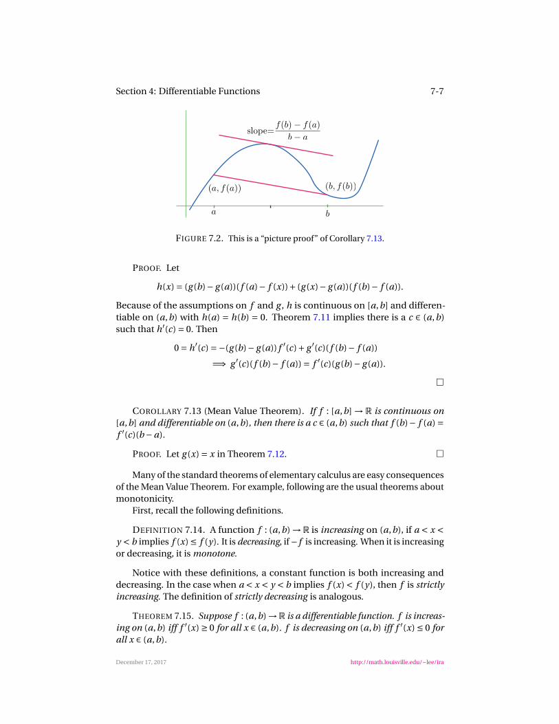
Section 4: Differentiable Functions 7-7
FIGURE 7.2. This is a “picture proof” of Corollary 7.13.
PROOF. Let
h(x) = (g (b)° g (a))( f (a)° f (x))+ (g (x)° g (a))( f (b)° f (a)).
Because of the assumptions on f and g , h is continuous on [a,b] and differen-tiable on (a,b) with h(a) = h(b) = 0. Theorem 7.11 implies there is a c 2 (a,b)such that h
0(c) = 0. Then
0 = h0(c) =°(g (b)° g (a)) f
0(c)+ g0(c)( f (b)° f (a))
=) g0(c)( f (b)° f (a)) = f
0(c)(g (b)° g (a)).
⇤
COROLLARY 7.13 (Mean Value Theorem). If f : [a,b] ! R is continuous on
[a,b] and differentiable on (a,b), then there is a c 2 (a,b) such that f (b)° f (a) =f0(c)(b °a).
PROOF. Let g (x) = x in Theorem 7.12. ⇤
Many of the standard theorems of elementary calculus are easy consequencesof the Mean Value Theorem. For example, following are the usual theorems aboutmonotonicity.
First, recall the following definitions.
DEFINITION 7.14. A function f : (a,b) ! R is increasing on (a,b), if a < x <y < b implies f (x) ∑ f (y). It is decreasing, if ° f is increasing. When it is increasingor decreasing, it is monotone.
Notice with these definitions, a constant function is both increasing anddecreasing. In the case when a < x < y < b implies f (x) < f (y), then f is strictly
increasing. The definition of strictly decreasing is analogous.
THEOREM 7.15. Suppose f : (a,b) !R is a differentiable function. f is increas-
ing on (a,b) iff f0(x) ∏ 0 for all x 2 (a,b). f is decreasing on (a,b) iff f
0(x) ∑ 0 for
all x 2 (a,b).
December 17, 2017 http://math.louisville.edu/ªlee/ira
7-8 CHAPTER 7. DIFFERENTIATION
PROOF. Only the first assertion is proved because the proof of the second ispretty much the same with all the inequalities reversed.
()) If x, y 2 (a,b) with x 6= y , then the assumption that f is increasing gives
f (y)° f (x)y °x
∏ 0 =) f0(x) = lim
y!x
f (y)° f (x)y °x
∏ 0.
(() Let x, y 2 (a,b) with x < y . According to Theorem 7.13, there is a c 2 (x, y)such that f (y)° f (x) = f
0(c)(y °x) ∏ 0. This shows f (x) ∑ f (y), so f is increasingon (a,b). ⇤
COROLLARY 7.16. Let f : (a,b) !R be a differentiable function. f is constant
iff f0(x) = 0 for all x 2 (a,b).
It follows from Theorem 7.2 that every differentiable function is continuous.But, it’s not true that a derivative must be continuous.
EXAMPLE 7.5. Let
f (x) =(
x2 sin 1
x, x 6= 0
0, x = 0.
We claim f is differentiable everywhere, but f0 is not continuous.
To see this, first note that when x 6= 0, the standard differentiation formulasgive that f
0(x) = 2x sin(1/x)°cos(1/x). To calculate f0(0), choose any h 6= 0. Then
ØØØØf (h)
h
ØØØØ=ØØØØ
h2 sin(1/h)
h
ØØØØ∑ØØØØ
h2
h
ØØØØ= |h|
and it easily follows from the definition of the derivative and the Squeeze Theorem(Theorem 6.3) that f
0(0) = 0.Therefore,
f0(x) =
(0, x = 0
2x sin 1x°cos 1
x, x 6= 0
.
Let xn = 1/2ºn for n 2N. Then xn ! 0 and
f0(xn) = 2xn sin(1/xn)°cos(1/xn)
= 1ºn
sin2ºn °cos2ºn =°1
for all n. Therefore, f0(xn) !°1 6= 0 = f
0(0), and f0 is not continuous at 0.
But, derivatives do share one useful property with continuous functions; theysatisfy an intermediate value property. Compare the following theorem withCorollary 6.26.
THEOREM 7.17 (Darboux’s Theorem). If f is differentiable on an open set
containing [a,b] and ∞ is between f0(a) and f
0(b), then there is a c 2 [a,b] such
that f0(c) = ∞.
PROOF. If f0(a) = f
0(b), then c = a satisfies the theorem. So, we may as wellassume f
0(a) 6= f0(b). There is no generality lost in assuming f
0(a) < f0(b), for,
otherwise, we just replace f with g =° f .
December 17, 2017 http://math.louisville.edu/ªlee/ira
5. APPLICATIONS OF THE MEAN VALUE THEOREM 7-9
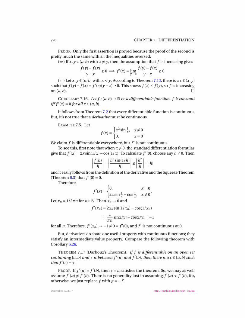
FIGURE 7.3. This could be the function h of Theorem 7.17.
Let h(x) = f (x)°∞x so that D( f ) = D(h) and h0(x) = f
0(x)°∞. In particular,this implies h
0(a) < 0 < h0(b). Because of this, there must be an "> 0 small enough
so thath(a +")°h(a)
"< 0 =) h(a +") < h(a)
andh(b)°h(b °")
"> 0 =) h(b °") < h(b).
(See Figure 7.3.) In light of these two inequalities and Theorem 6.23, there mustbe a c 2 (a,b) such that h(c) = glb{h(x) : x 2 [a,b]}. Now Theorem 7.9 gives 0 =h0(c) = f
0(c)°∞, and the theorem follows. ⇤Here’s an example showing a possible use of Theorem 7.17.
EXAMPLE 7.6. Let
f (x) =(
0, x 6= 0
1, x = 0.
Theorem 7.17 implies f is not a derivative.
A more striking example is the following
EXAMPLE 7.7. Define
f (x) =(
sin 1x
, x 6= 0
1, x = 0and g (x) =
(sin 1
x, x 6= 0
°1, x = 0.
Since
f (x)° g (x) =(
0, x 6= 0
2, x = 0
does not have the intermediate value property, at least one of f or g is not aderivative. (Actually, neither is a derivative because f (x) =°g (°x).)
5. Applications of the Mean Value Theorem
In the following sections, the standard notion of higher order derivativesis used. To make this precise, suppose f is defined on an interval I . Thefunction f itself can be written f
(0). If f is differentiable, then f0 is written
f(1). Continuing inductively, if n 2 !, f
(n) exists on I and x0 2 D( f(n)), then
f(n+1)(x0) = d f
(n)(x0)/d x.
5December 17, 2017 ©Lee Larson ([email protected])
December 17, 2017 http://math.louisville.edu/ªlee/ira
7-10 CHAPTER 7. DIFFERENTIATION
5.1. Taylor’s Theorem. The motivation behind Taylor’s theorem is the at-tempt to approximate a function f near a number a by a polynomial. Thepolynomial of degree 0 which does the best job is clearly p0(x) = f (a). Thebest polynomial of degree 1 is the tangent line to the graph of the functionp1(x) = f (a)+ f
0(a)(x ° a). Continuing in this way, we approximate f near a
by the polynomial pn of degree n such that f(k)(a) = p
(k)n (a) for k = 0,1, . . . ,n. A
simple induction argument shows that
(7.6) pn(x) =nX
k=0
f(k)(a)k !
(x °a)k .
This is the well-known Taylor polynomial of f at a.Many students leave calculus with the mistaken impression that (7.6) is the
important part of Taylor’s theorem. But, the important part of Taylor’s theoremis the fact that in many cases it is possible to determine how large n must be toachieve a desired accuracy in the approximation of f ; i. e., the error term is theimportant part.
THEOREM 7.18 (Taylor’s Theorem). If f is a function such that f , f0, . . . , f
(n)
are continuous on [a,b] and f(n+1)
exists on (a,b), then there is a c 2 (a,b) such
that
f (b) =nX
k=0
f(k)(a)k !
(b °a)k + f(n+1)(c)
(n +1)!(b °a)n+1.
PROOF. Let the constant Æ be defined by
(7.7) f (b) =nX
k=0
f(k)(a)k !
(b °a)k + Æ
(n +1)!(b °a)n+1
and define
F (x) = f (b)°√
nX
k=0
f(k)(x)k !
(b °x)k + Æ
(n +1)!(b °x)n+1
!
.
From (7.7) we see that F (a) = 0. Direct substitution in the definition of F showsthat F (b) = 0. From the assumptions in the statement of the theorem, it is easy tosee that F is continuous on [a,b] and differentiable on (a,b). An application ofRolle’s Theorem yields a c 2 (a,b) such that
0 = F0(c) =°
µf
(n+1)(c)n!
(b ° c)n ° Æ
n!(b ° c)n
∂=) Æ= f
(n+1)(c),
as desired. ⇤
Now, suppose f is defined on an open interval I with a, x 2 I . If f is n +1times differentiable on I , then Theorem 7.18 implies there is a c between a and x
such that
f (x) = pn(x)+R f (n, x, a),
December 17, 2017 http://math.louisville.edu/ªlee/ira
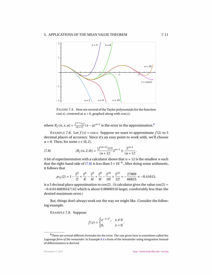
5. APPLICATIONS OF THE MEAN VALUE THEOREM 7-11
2 4 6 8
-4
-2
2
4
n = 2
n = 4
n = 6
n = 8
n = 10
n = 20
y = cos(x)
FIGURE 7.4. Here are several of the Taylor polynomials for the functioncos(x), centered at a = 0, graphed along with cos(x).
where R f (n, x, a) = f(n+1)(c)(n+1)! (x °a)n+1 is the error in the approximation.6
EXAMPLE 7.8. Let f (x) = cos x. Suppose we want to approximate f (2) to 5decimal places of accuracy. Since it’s an easy point to work with, we’ll choosea = 0. Then, for some c 2 (0,2),
(7.8) |R f (n,2,0)| = | f (n+1)(c)|(n +1)!
2n+1 ∑ 2n+1
(n +1)!.
A bit of experimentation with a calculator shows that n = 12 is the smallest n suchthat the right-hand side of (7.8) is less than 5£10°6. After doing some arithmetic,it follows that
p12(2) = 1° 22
2!+ 24
4!° 26
6!+ 28
8!° 210
10!+ 212
12!=°27809
66825º°0.41615.
is a 5 decimal place approximation to cos(2). (A calculator gives the value cos(2) =°0.416146836547142 which is about 0.00000316 larger, comfortably less than thedesired maximum error.)
But, things don’t always work out the way we might like. Consider the follow-ing example.
EXAMPLE 7.9. Suppose
f (x) =(
e°1/x
2, x 6= 0
0, x = 0.
6There are several different formulas for the error. The one given here is sometimes called theLagrange form of the remainder. In Example 8.4 a form of the remainder using integration insteadof differentiation is derived.
December 17, 2017 http://math.louisville.edu/ªlee/ira
7-12 CHAPTER 7. DIFFERENTIATION
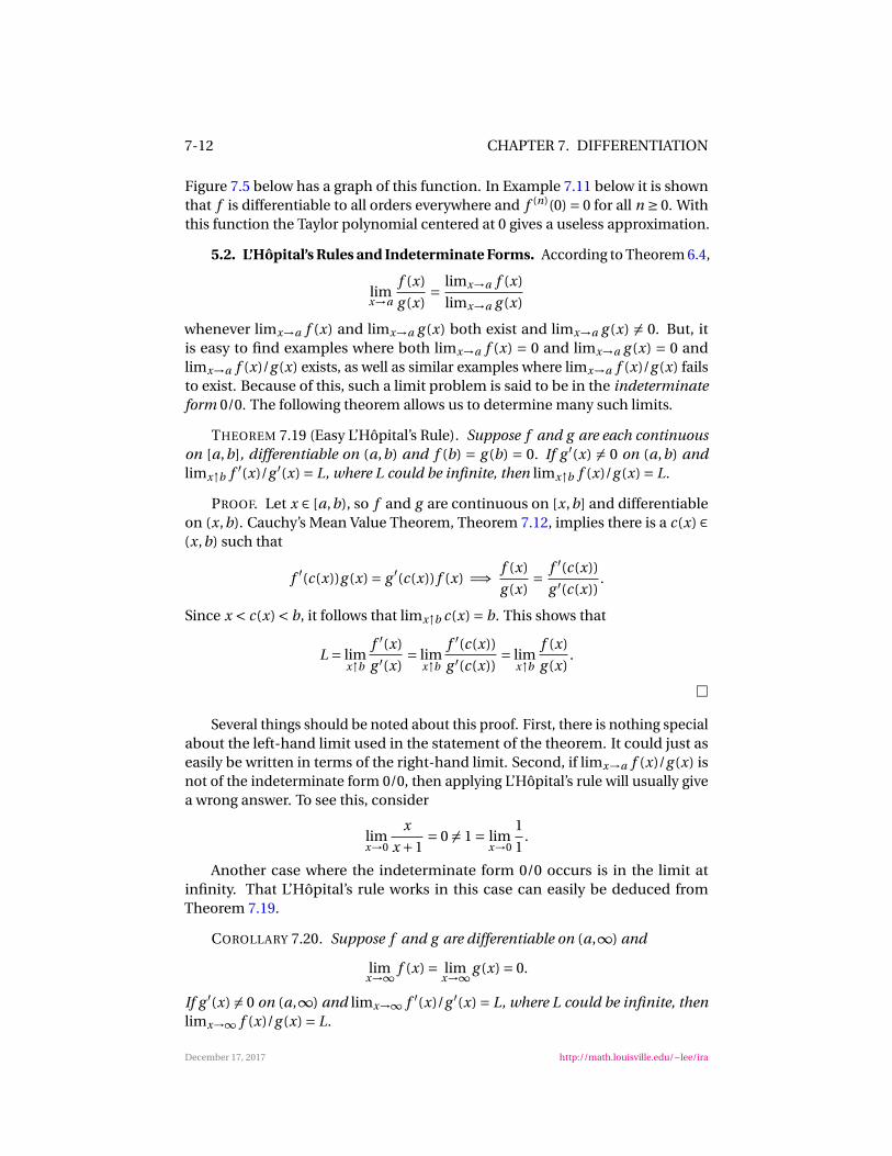
Figure 7.5 below has a graph of this function. In Example 7.11 below it is shownthat f is differentiable to all orders everywhere and f
(n)(0) = 0 for all n ∏ 0. Withthis function the Taylor polynomial centered at 0 gives a useless approximation.
5.2. L’Hôpital’s Rules and Indeterminate Forms. According to Theorem 6.4,
limx!a
f (x)g (x)
= limx!a f (x)limx!a g (x)
whenever limx!a f (x) and limx!a g (x) both exist and limx!a g (x) 6= 0. But, itis easy to find examples where both limx!a f (x) = 0 and limx!a g (x) = 0 andlimx!a f (x)/g (x) exists, as well as similar examples where limx!a f (x)/g (x) failsto exist. Because of this, such a limit problem is said to be in the indeterminate
form 0/0. The following theorem allows us to determine many such limits.
THEOREM 7.19 (Easy L’Hôpital’s Rule). Suppose f and g are each continuous
on [a,b], differentiable on (a,b) and f (b) = g (b) = 0. If g0(x) 6= 0 on (a,b) and
limx"b f0(x)/g
0(x) = L, where L could be infinite, then limx"b f (x)/g (x) = L.
PROOF. Let x 2 [a,b), so f and g are continuous on [x,b] and differentiableon (x,b). Cauchy’s Mean Value Theorem, Theorem 7.12, implies there is a c(x) 2(x,b) such that
f0(c(x))g (x) = g
0(c(x)) f (x) =) f (x)g (x)
= f0(c(x))
g 0(c(x)).
Since x < c(x) < b, it follows that limx"b c(x) = b. This shows that
L = limx"b
f0(x)
g 0(x)= lim
x"b
f0(c(x))
g 0(c(x))= lim
x"b
f (x)g (x)
.
⇤
Several things should be noted about this proof. First, there is nothing specialabout the left-hand limit used in the statement of the theorem. It could just aseasily be written in terms of the right-hand limit. Second, if limx!a f (x)/g (x) isnot of the indeterminate form 0/0, then applying L’Hôpital’s rule will usually givea wrong answer. To see this, consider
limx!0
x
x +1= 0 6= 1 = lim
x!0
11
.
Another case where the indeterminate form 0/0 occurs is in the limit atinfinity. That L’Hôpital’s rule works in this case can easily be deduced fromTheorem 7.19.
COROLLARY 7.20. Suppose f and g are differentiable on (a,1) and
limx!1
f (x) = limx!1
g (x) = 0.
If g0(x) 6= 0 on (a,1) and limx!1 f
0(x)/g0(x) = L, where L could be infinite, then
limx!1 f (x)/g (x) = L.
December 17, 2017 http://math.louisville.edu/ªlee/ira
5. APPLICATIONS OF THE MEAN VALUE THEOREM 7-13
PROOF. There is no generality lost by assuming a > 0. Let
F (x) =(
f (1/x), x 2 (0,1/a]
0, x = 0and G(x) =
(g (1/x), x 2 (0,1/a]
0, x = 0.
Thenlimx#0
F (x) = limx!1
f (x) = 0 = limx!1
g (x) = limx#0
G(x),
so both F and G are continuous at 0. It follows that both F and G are continuouson [0,1/a] and differentiable on (0,1/a) with G
0(x) =°g0(1/x)/x
2 6= 0 on (0,1/a)and limx#0 F
0(x)/G0(x) = limx!1 f
0(x)/g0(x) = L. The rest follows from Theorem
7.19. ⇤The other standard indeterminate form arises when
limx!1
f (x) =1= limx!1
g (x).
This is called an 1/1 indeterminate form. It is often handled by the followingtheorem.
THEOREM 7.21 (Hard L’Hôpital’s Rule). Suppose that f and g are differentiable
on (a,1) and g0(x) 6= 0 on (a,1). If
limx!1
f (x) = limx!1
g (x) =1 and limx!1
f0(x)
g 0(x)= L 2R[ {°1,1},
then
limx!1
f (x)g (x)
= L.
PROOF. First, suppose L 2R and let "> 0. Choose a1 > a large enough so thatØØØØ
f0(x)
g 0(x)°L
ØØØØ< ", 8x > a1.
Since limx!1 f (x) =1= limx!1 g (x), we can assume there is an a2 > a1 suchthat both f (x) > 0 and g (x) > 0 when x > a2. Finally, choose a3 > a2 such thatwhenever x > a3, then f (x) > f (a2) and g (x) > g (a2).
Let x > a3 and apply Cauchy’s Mean Value Theorem, Theorem 7.12, to f andg on [a2, x] to find a c(x) 2 (a2, x) such that
(7.9)f0(c(x))
g 0(c(x))= f (x)° f (a2)
g (x)° g (a2)=
f (x)≥1° f (a2)
f (x)
¥
g (x)≥1° g (a2)
g (x)
¥ .
If
h(x) =1° g (a2)
g (x)
1° f (a2)f (x)
,
then (7.9) impliesf (x)g (x)
= f0(c(x))
g 0(c(x))h(x).
December 17, 2017 http://math.louisville.edu/ªlee/ira
7-14 CHAPTER 7. DIFFERENTIATION
Since limx!1 h(x) = 1, there is an a4 > a3 such that whenever x > a4, then |h(x)°1| < ". If x > a4, then
ØØØØf (x)g (x)
°L
ØØØØ=ØØØØ
f0(c(x))
g 0(c(x))h(x)°L
ØØØØ
=ØØØØ
f0(c(x))
g 0(c(x))h(x)°Lh(x)+Lh(x)°L
ØØØØ
∑ØØØØ
f0(c(x))
g 0(c(x))°L
ØØØØ |h(x)|+ |L||h(x)°1|
< "(1+")+|L|"= (1+|L|+")"
can be made arbitrarily small through a proper choice of ". Therefore
limx!1
f (x)/g (x) = L.
The case when L =1 is done similarly by first choosing a B > 0 and adjusting(7.9) so that f
0(x)/g0(x) > B when x > a1. A similar adjustment is necessary when
L =°1. ⇤There is a companion corollary to Theorem 7.21 which is proved in the same
way as Corollary 7.20.
COROLLARY 7.22. Suppose that f and g are continuous on [a,b] and differen-
tiable on (a,b) with g0(x) 6= 0 on (a,b). If
limx#a
f (x) = limx#a
g (x) =1 and limx#a
f0(x)
g 0(x)= L 2R[ {°1,1},
then
limx#a
f (x)g (x)
= L.
EXAMPLE 7.10. If Æ > 0, then limx!1 ln x/xÆ is of the indeterminate form
1/1. Taking derivatives of the numerator and denominator yields
limx!1
1/x
ÆxÆ°1 = limx!1
1ÆxÆ
= 0.
Theorem 7.21 now implies limx!1 ln x/xÆ = 0, and therefore ln x increases more
slowly than any positive power of x.
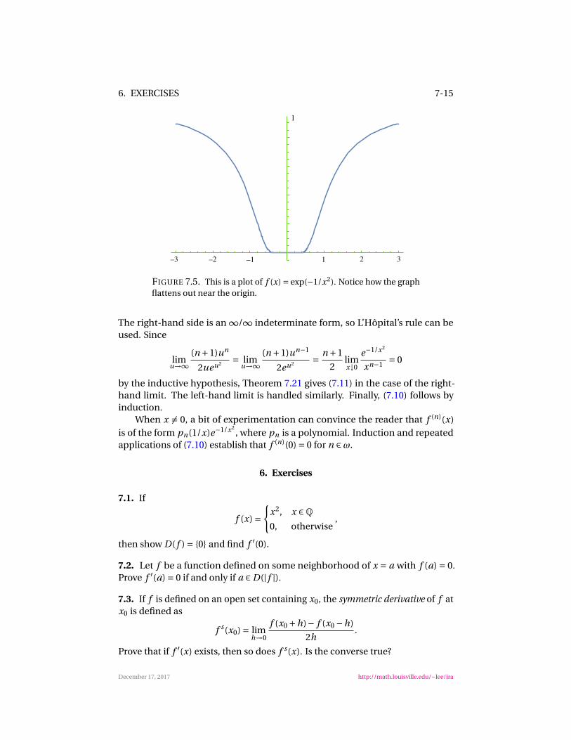
EXAMPLE 7.11. Let f be as in Example 7.9. (See Figure 7.5.) It is clear f(n)(x)
exists whenever n 2! and x 6= 0. We claim f(n)(0) = 0. To see this, we first prove
that
limx!0
e°1/x
2
xn= 0, 8n 2Z.(7.10)
When n ∑ 0, (7.10) is obvious. So, suppose (7.10) is true whenever m ∑ n forsome n 2!. Making the substitution u = 1/x, we see
limx#0
e°1/x
2
xn+1 = limu!1
un+1
eu2 .(7.11)
December 17, 2017 http://math.louisville.edu/ªlee/ira
6. EXERCISES 7-15
!"
–2 –1 1 2 3
1
–3
FIGURE 7.5. This is a plot of f (x) = exp(°1/x2). Notice how the graph
flattens out near the origin.
The right-hand side is an 1/1 indeterminate form, so L’Hôpital’s rule can beused. Since
limu!1
(n +1)un
2ueu2 = limu!1
(n +1)un°1
2eu2 = n +12
limx#0
e°1/x
2
xn°1 = 0
by the inductive hypothesis, Theorem 7.21 gives (7.11) in the case of the right-hand limit. The left-hand limit is handled similarly. Finally, (7.10) follows byinduction.
When x 6= 0, a bit of experimentation can convince the reader that f(n)(x)
is of the form pn(1/x)e°1/x
2, where pn is a polynomial. Induction and repeated
applications of (7.10) establish that f(n)(0) = 0 for n 2!.
6. Exercises
7.1. If
f (x) =(
x2, x 2Q
0, otherwise,
then show D( f ) = {0} and find f0(0).
7.2. Let f be a function defined on some neighborhood of x = a with f (a) = 0.Prove f
0(a) = 0 if and only if a 2 D(| f |).
7.3. If f is defined on an open set containing x0, the symmetric derivative of f atx0 is defined as
fs(x0) = lim
h!0
f (x0 +h)° f (x0 °h)2h
.
Prove that if f0(x) exists, then so does f
s(x). Is the converse true?
December 17, 2017 http://math.louisville.edu/ªlee/ira
7-16 CHAPTER 7. DIFFERENTIATION
7.4. Let G be an open set and f 2 D(G). If there is an a 2G such that limx!a f0(x)
exists, then limx!a f0(x) = f
0(a).
7.5. Suppose f is continuous on [a,b] and f00 exists on (a,b). If there is an
x0 2 (a,b) such that the line segment between (a, f (a)) and (b, f (b)) contains thepoint (x0, f (x0)), then there is a c 2 (a,b) such that f
00(c) = 0.
7.6. If ¢ = { f : f = F0 for some F : R! R}, then ¢ is closed under addition and
scalar multiplication. (This shows the derivatives form a vector space.)
7.7. If
f1(x) =(
1/2, x = 0
sin(1/x), x 6= 0
and
f2(x) =(
1/2, x = 0
sin(°1/x), x 6= 0,
then at least one of f1 and f2 is not in ¢.
7.8. Prove or give a counter example: If f is continuous on R and differentiableon R\ {0} with limx!0 f
0(x) = L, then f is differentiable on R.
7.9. Suppose f is differentiable everywhere and f (x+y) = f (x) f (y) for all x, y 2R.Show that f
0(x) = f0(0) f (x) and determine the value of f
0(0).
7.10. If I is an open interval, f is differentiable on I and a 2 I , then there is asequence an 2 I \ {a} such that an ! a and f
0(an) ! f0(a).
7.11. Use the definition of the derivative to findd
d x
px.
7.12. Let f be continuous on [0,1) and differentiable on (0,1). If f (0) = 0 and| f 0(x)|∑ | f (x)| for all x > 0, then f (x) = 0 for all x ∏ 0.
7.13. Suppose f : R! R is such that f0 is continuous on [a,b]. If there is a
c 2 (a,b) such that f0(c) = 0 and f
00(c) > 0, then f has a local minimum at c.
7.14. Prove or give a counter example: If f is continuous on R and differentiableon R\ {0} with limx!0 f
0(x) = L, then f is differentiable on R.
7.15. Let f be continuous on [a,b] and differentiable on (a,b). If f (a) =Æ and| f 0(x)| <Ø for all x 2 (a,b), then calculate a bound for f (b).
7.16. Suppose that f : (a,b) ! R is differentiable and f0 is bounded. If xn is a
sequence from (a,b) such that xn ! a, then f (xn) converges.
7.17. Let G be an open set and f 2 D(G). If there is an a 2G such that limx!a f0(x)
exists, then limx!a f0(x) = f
0(a).
December 17, 2017 http://math.louisville.edu/ªlee/ira
6. EXERCISES 7-17
7.18. Prove or give a counter example: If f 2 D((a,b)) such that f0 is bounded,
then there is an F 2C ([a,b]) such that f = F on (a,b).
7.19. Show that f (x) = x3 +2x +1 is invertible on R and, if g = f
°1, then findg0(1).
7.20. Suppose that I is an open interval and that f00(x) ∏ 0 for all x 2 I . If a 2 I ,
then show that the part of the graph of f on I is never below the tangent line tothe graph at (a, f (a)).
7.21. Suppose f is continuous on [a,b] and f00 exists on (a,b). If there is an
x0 2 (a,b) such that the line segment between (a, f (a)) and (b, f (b)) contains thepoint (x0, f (x0)), then there is a c 2 (a,b) such that f
00(c) = 0.
7.22. Let f be defined on a neighborhood of x.
(a) If f00(x) exists, then
limh!0
f (x °h)°2 f (x)+ f (x +h)h2 = f
00(x).
(b) Find a function f where this limit exists, but f00(x) does not exist.
7.23. If f : R! R is differentiable everywhere and is even, then f0 is odd. If
f :R!R is differentiable everywhere and is odd, then f0 is even.7
7.24. Prove that ØØØØsin x °µ
x ° x3
6+ x
5
120
∂ØØØØ<1
5040when |x|∑ 1.
7.25. The exponential function ex is not a polynomial.
7A function g is even if g (°x) = g (x) for every x and it is odd if g (°x) =°g (x) for every x. Evenand odd functions are described as such because this is how g (x) = x
n behaves when n is an evenor odd integer, respectively.
December 17, 2017 http://math.louisville.edu/ªlee/ira
Top Related