


Languages
Pages
Legal

Chalmers University of Technology University of Gothenburg Department of Computer Science and Engineering Göteborg, Sweden, March 2015
Developing high performance database
clusters in MongoDB Master of Science Thesis in Software Engineering
ERIC LUNDGREN
The Author grants to Chalmers University of Technology and
University of Gothenburg the non-exclusive right to publish the
Work electronically and in a non-commercial purpose make it
accessible on the Internet.
The Author warrants that he/she is the author to the Work, and
warrants that the Work does not contain text, pictures or other
material that violates copyright law.
The Author shall, when transferring the rights of the Work to a third
party (for example a publisher or a company), acknowledge the
third party about this agreement. If the Author has signed a
copyright agreement with a third party regarding the Work, the
Author warrants hereby that he/she has obtained any necessary
permission from this third party to let Chalmers University of
Technology and University of Gothenburg store the Work
electronically and make it accessible on the Internet.
Developing high performance database cluster in MongoDB
ERIC N. D. LUNDGREN
© ERIC N. D. LUNDGREN, March 2015.
Supervisor: GRAHAM J.L. KEMP
Examiner: AGNETA NILSSON
Chalmers University of Technology
University of Gothenburg
Department of Computer Science and Engineering
SE-412 96 Göteborg
Sweden
Telephone + 46 (0)31-772 1000
Department of Computer Science and Engineering
Göteborg, Sweden March 2015

Table of Contents 1 Introduction ......................................................................................................... 5
2 Background .......................................................................................................... 7
2.1 Radish ............................................................................................................. 8
2.2 NoSQL and MongoDB .............................................................................. 8
2.3 Virtual Machines ........................................................................................ 9
2.4 Benchmarking........................................................................................... 10
2.4.1 Hardware Aspects ......................................................................... 10
2.4.2 Workload Considerations .......................................................... 11
3 Method .................................................................................................................. 12
3.1 Virtual Machine Environment........................................................... 12
3.2 Benchmarking Tool ................................................................................ 14
3.3 Workload..................................................................................................... 15
3.3.1 Social Networking Illusion ........................................................ 17
4 Result..................................................................................................................... 19
4.1 Iteration 1 ................................................................................................... 22
4.2 Iteration 2 ................................................................................................... 23
4.3 Iteration 3 ................................................................................................... 25
4.4 Iteration 4 ................................................................................................... 26
4.5 Iteration 5 ................................................................................................... 27
4.6 Iteration 6 ................................................................................................... 29
4.7 Iteration 7 ................................................................................................... 31
4.8 Iteration 8 ................................................................................................... 32
4.9 Iteration 9 ................................................................................................... 35
5 Delimitations & Problems ........................................................................... 36
5.1 Method ......................................................................................................... 36
5.2 Technical ..................................................................................................... 36
5.3 Current Use Case ..................................................................................... 37
6 Discussion ........................................................................................................... 38
6.1 Related Work ............................................................................................ 38
6.2 Ethical Considerations .......................................................................... 39
6.3 DBMS Comparisons ................................................................................ 40
6.4 Future Work .............................................................................................. 40
7 Conclusion .......................................................................................................... 42
References .................................................................................................................... 43
Appendix A ................................................................................................................... 46

4
Result 4.1 .................................................................................................................. 46
Result 4.2 .................................................................................................................. 47
Result 4.3 .................................................................................................................. 49
Result 4.4 .................................................................................................................. 51
Result 4.5 .................................................................................................................. 53
Result 4.6 .................................................................................................................. 55
5
1 Introduction
This report describes the design and development of a database cluster in
MongoDB and a method of tuning the cluster for maximum performance to a
particular use case. Database clusters can have a lot of different setups or
designs which all have a different impact on how well the cluster is able to
handle certain data and queries. Designing the best database cluster is an
intractable problem as the optimal design, to a large extent, depends on the
particular use case. Furthermore, given the size and complexity of a DBMS, it
is virtually impossible to prove the design of a cluster as optimal. These two
facts explain why there are no formal methods of how to design the best
possible database cluster. Chodorow (2011) in her book Scaling MongoDB
tries to give general advice on how to work with clusters in MongoDB but it
typically comes down to the fact that it’s very application specific. For example
when asked what sharding key should be used, she states “Not knowing your
application, I can’t really tell you.” (Chodorow, 2011, p. 24).
The main problem tackled in this report will be to provide a way of
systematically achieving a design as close as possible to the optimal design of
a database cluster. Once this has been established, a variety of sub problems
emerge related as to how this can be done in practice and in a general case
through the use of virtualization technologies and cluster benchmarking.
As storage is a crucial component in many computer systems, this research is
highly necessary as it could aide both research institutions and businesses in
designing database clusters that performs better for their particular use cases.
There is research that has gone into establishing general guidelines of how
databases such as MongoDB should be used (Stonebraker and Cattell, 2010),
but no technique has been established as how to design the best possible
database cluster.
Hevner et al. (2004) states that design is both a process and a product. This
research will describe the process to achieve a design that best tackles a
certain use case. The use case used in this report is tied to that of a particular
social networking app, but this report will provide the tools and methods
necessary for the reader to optimize and compare cluster designs in any
arbitrary setting.
In order to compare designs of database clusters, it is imperative to have
something quantifiable that defines the cluster’s performance. The term
performance is subjective, but in this report it will refer to the number of
simple queries that can be handled by a particular cluster within some time
interval. This number will vary a lot for different use cases even if the same

6
cluster setup is used, so comparing setups across different use cases will not
be considered in this report.
Hevner et al. (2004) states that design is inherently an iterative and
incremental activity. Because of this, I have in my approach taken inspiration
from the design-science paradigm which aims to solve problems of an
intractable and wicked nature (Hevner et al. 2004). Throughout this report I
will be using an approach based on benchmarking the performance of
different cluster setups. By simulating a workload of my particular use case or
production environment, I will be able to measure how well the cluster is able
to perform during these circumstances. Then through using the search process
method from the design-science paradigm, I can use heuristics to change the
cluster setup systematically in order to find as good a setup as possible.
7
2 Background
Trying to optimize databases and making them better at utilizing their hardware resources has been going on ever since the introduction of databases. There are best practices one can follow when designing datastores in the SQL world (Harrington, 2002). However little to no research exists around how to design databases and database clusters for document stores like MongoDB. Within the scientific community there is however a clearly defined way of how measuring the performance of a document store can be done (Cooper et al. 2010) and with that, also comes the possibility to compare document stores to each other (Cooper et al. 2010). This has been going on for some time, both with document stores and those from the SQL world, to compare the performance of different DBMSs towards each other (Cooper et al. 2010). This technique of comparing benchmarks to each other is what I plan to utilize in my research. There are however a few distinct differences - I shall only be using one DBMS, a document store called MongoDB, and focus primarily on a clustered environment rather than a single database instance. The comparisons should then be made between different types of cluster designs in order to find out how they affect the performance. Upon seeing this, it should be possible to deduce different hypotheses regarding the design that may improve the performance of the cluster even further. This leads to a variety of scientific challenges as the different hypotheses needs to be tested, analyzed and verified. I have chosen to do this through adapting some of the strategies used in quantitative trading and build my own framework around the testing and verification. The idea behind quantitative trading is to prove or disprove optimizations to your trading strategy through simulation or algebra. This can be done continuously in order to achieve as good a strategy as possible. A similar pattern or workflow can also be seen in the design-science paradigm. In its simplest form it can be described as an iterative process with two steps, the developing phase and the evaluating phase (Hevner et al. 2004). You build an artifact or a system as part of the investigation and refine it, for instance, through heuristics found in the evaluating phase. This is known as a search process (Hevner et al. 2004). Implementing this brings with it a large set of engineering challenges such as adapting existing benchmarking frameworks to work on clusters, automatically being able to generate clusters of different setups, computing on large and changing data together with accounting for the complex environment around the DBMSs. The goal upon solving these challenges is that this research will provide the reader with an alternative way of designing a high performing database cluster in MongoDB. The reader shall also have seen how this works in practice and understand why it works. Furthermore, the reader should also have the
8
knowledge and tools to apply this alternative method of designing a database cluster to his or her own use case. In order to fully appreciate and understand this method, some key aspects, elements and terms must be clearly defined as explained below. 2.1 Radish
Radish is a tech-startup based in Gothenburg, Sweden. Their main product is
a photo collecting iPhone app called MeBox.
MeBox makes pictures of yourself, taken by other people using MeBox,
available to you even though they are taken by a device other than your own.
Today it works by a face recognition algorithm that upon inspecting a photo,
firstly determines if there are individuals in the photo. If there are individuals
in the photo, the algorithm provides you with suggestions of who the
person(s) might be. The user is then free to select from these suggestions and
any other people stored in some way on the phone and tag them in the photo.
If that person is a user of the app, this would make the photo accessible to
them. It accesses your personal information such as Facebook contacts,
address book and other photos in your phone to provide these suggestions of
individuals. It is intended for the face recognition algorithm to eventually take
peoples geographical location into account when matching faces. There is also
a plan to eventually allow automatic tagging where the face recognition
algorithm fully determines who is in a photo.
This is the production use case which will be used as an example when
illustrating the optimization method later on.
2.2 NoSQL and MongoDB
There are many different kinds of NoSQL databases but they have in common
that they typically process data quicker than relational databases and also
scale better (Cattell, 2010). Some of the NoSQL databases are also able to scale
horizontally, or in other words run distributed over several machines. This
comes at a cost in the atomicity domain but as long as your application can
endure an “eventually consistent” level of atomicity – there is potential for a
great performance increase in using this horizontal scaling (Cattell, 2010). The
“eventually consistent” level of atomicity means that changes to data on one
machine will sooner or later propagate to other machines in the cluster.
However it leaves room for the data to not be consistent for a short period of
time after changes to it has been made.
MongoDB is what is referred to as a document store (The MongoDB 2.4
Manual, 2014). The term document store may be confusing and it also goes
9
under the name document oriented database. The documents here do not
refer to documents in the traditional sense but to any kind of “pointerless
object” (Cattell, 2010). They store unstructured data which can be nested and
provide a simple querying interface (Cattell, 2010).
There is a generic term for dividing data in a database called partitioning. This
can be done in several ways and one of them is referred to as horizontal
partitioning or sharding. This is the technique used by MongoDB to achieve
horizontal scalability and in this report I will use the term sharding as it is the
term used in MongoDB’s documentation.
Sharding is a technique where you take large datasets and divide them into
smaller pieces, referred to as shards, by some field of the data referred to as
the sharding key (Chodorow, 2011). An example could be that we have a
collection of users and choose their last names as a sharding key. We will now
divide the user collection into smaller pieces (shards) by using the last names
of the elements. This can be done in several ways, for instance by using a
range-based approach where we arrange the elements in a lexicographical
order on their last names and divide the collection into however many shards
we want. Another way is to apply a hashing function on the chosen field and
then use the modulo operator to decide in which shard an element belongs.
2.3 Virtual Machines
Today’s machines are sufficiently powerful to use virtualization in order to
present the illusion of a smaller, virtual machine, running its own operating
system (Barham et al. 2003). The concept of virtualization was first coined in
the 1960’s by IBM. But it wasn’t until more recently when machines got
powerful enough and the technology was improved upon that it gained more
traction (Younge et al. 2011).
Younge et al. states that virtualization in its simplest form is a mechanism to
abstract the hardware and the system resources from the operating system.
Many tools and frameworks for virtualization have been developed and they
typically work through the use of a hypervisor or VMM (Virtual Machine
Monitor) (Younge et al. 2011) (Groesbrink et al. 2014). The hypervisor works
by taking the instructions from the VMs and their simulated hardware and has
them execute on the host’s hardware instead (Younge et al. 2011) (Groesbrink
et al. 2014).
Younge et al. states that the use of virtualization technologies has increased
dramatically in the past few years and that it’s also one of the most important
underlying technologies of cloud computing. This is due to the fact that the
hypervisors enable computing resources to be spread out as seen fit between
10
the different VMs and also allows them to be modified with great ease. A lot of
research is still going into virtualization and particularly the hypervisors.
There’s an ongoing race between the different large vendors such as Xen,
VMware and VirtualBox to support more and more computing resources and
allow for more virtual CPUs (Younge et al. 2011). There is also state of the art
research going into supporting dynamic resource management (Groesbrink et
al. 2014). VMware alone has seen a continuous increase in the number of
approved patents ever since 2011 (Freshpatents.com, 2014) and there’s also
research going into making the best usage of virtualized environments (Liu,
2014) (Hsieh, 2008). The concept of virtualization has even spread from just
virtualizing hardware to virtualizing data (Delphix Corp. 2009).
My choice of virtualization environment fell on VMware ESXi which is an
operating system for hosting virtual machines. It is very lightweight and
consumes only minimal resources in order to be able to distribute its
hardware resources to its hosted machines. Unlike most other virtualization
environments, the hypervisor in ESXi also provides its users with the
possibility of allocating CPU computing time. This is done through a CPU
scheduler that runs in the host machine. After a virtual machine has been
created, you specify how many of the host’s CPU cores the VM should have
access to. The computation power of these cores in terms of MHz are then
viewed as a resource pool, and during runtime, the scheduler partitions the
use of the physical CPU to ensure that it spends the right amount of time on
each virtual machine. Tests have been carried out to ensure that this feature
achieved fair distributions of CPU resources and that machines with reserved
CPU resources are not compromised by heavy loads on other VMs or the host
machine (VMware Inc, 2013).
2.4 Benchmarking
2.4.1 Hardware Aspects
One of the most crucial things when it comes to benchmarking is to choose an
appropriate measurement. Rubenstein et al. (1987) defined the appropriate
measurement to their benchmarking experiment as the response time in
milliseconds. They chose this because of the fact that it is the measurement
that is most critical to the actual applications using the database. They go on
to explain that this measurement makes the results very dependent on the
hardware specifications on the system running the benchmarking as opposed
to if they would use the CPU time. However, it is debatable whether this would
eliminate that problem either as different CPUs are optimized for different
CPU instructions.
11
I choose to define an operation as an interaction with the database from some
application in the shape of either an insert, update, read or a scan following
the research of Cooper et al. (2010). Based on this I have chosen to focus on
the number of operations per second that can be handled by the database.
Essentially this is quite similar to measuring the response times from the client
side. The more operations per second that can be handled by the database, the
shorter the response times as seen from the application. However measuring
the response times also takes into account the potential overheads associated
with the client such as network latencies, process scheduling and disk
latencies to name a few. These factors will naturally play a part for me too,
however only on the database side where the MongoDB instances are running,
and not for the machines initiating the database operations.
This approach leads to the same dilemma as for Rubenstein et al., that the
results produced become highly dependent on the hardware of the system.
However it will still be possible to compare results on different cluster setups
towards each other if they are run on identical hardware.
2.4.2 Workload Considerations
Rubenstein et al. (1987) benchmarks the use of simple database operations.
They define these simple database operations as lookups, range lookups,
group lookups, reference lookups, sequential scans and opening of databases.
This research uses a schema associated with relational databases but
following the use of denormalization which is a common technique in NoSQL,
this approach of using simple operations becomes even more suitable.
Because of the denormalization, the processes of getting the data is generally
a bit easier than if you would have to, for instance, make joins and reference
lookups. The operations can now generally be divided into one of four possible
categories - inserts, updates, reads and scans (Cooper et al. 2010).
These operations can all be found in the work by Rubenstein et al. but renders
a few of the original operations obsolete, reference lookups being one of these.
It is important for the ratio between these four operations to be close to those
of the production environment for the results to be of any use. Previous
research has used separate workloads to test the systems for different types
of load distribution, in my case it is however possible to inspect the live
production machine. This gives me very good values on the distribution
between operations to use for my benchmarking. I will conduct my
benchmarking based on the distributions of the production environment in
conjunction with another slightly different distribution, in order to see how
this affects the properties of the database cluster.
12
3 Method
As previously mentioned, the method will follow a search-process from the
design-science paradigm (Hevner et al. 2004). An artifact will thus be acquired
as a part of the investigation and in my case be the final cluster design. My
adaptation of this method consists of three steps that are repeated, following
agile practices, to increase the level of quality of the resulting database cluster
through each iteration. The first step is to initialize a database cluster. This is
followed by applying a workload to this cluster and benchmarking the results.
After this there is an evaluation phase where the results of the benchmarking
are analyzed. Based on the results, there will lastly be a section describing
what to change in the cluster setup for the next iteration that may increase the
performance of the cluster even further.
In the end, this should give a cluster that is able to handle the simulated
workload very efficiently and as this workload represents the production
workload - it should also perform really well out in production.
3.1 Virtual Machine Environment
Database clusters can take many different shapes and there are many
important factors to consider. Attributes that define clusters include the
number of nodes in the cluster, the choice of sharding key, how many and
where to place replicated sets and many more. In order to quickly be able to
change these attributes it is not feasible to use physical machines. This would
require a lot of identical machines which would all have to be configured
individually. Instead, a design choice was taken to use Virtual Machines. The
machines to host the MongoDB clients are generated from a template to
ensure that they all have the same computing capabilities. They also all appear
in the same network and on the same host machine in order to as much as
possible avoid unevenly spread latencies.
As previously mentioned, the choice of virtualization technology fell on
VMware and their ESXi host. ESXi, given its lightweight nature, is merely a
system for hosting VMs and not to manage them. In order to be able to do
meaningful things with the VMs that are running on ESXi, a separate service
called vCenter is needed. This service allows you to connect to the host
operating system, open up terminals to the existing virtual machines, create
templates, clone machines and much more.
VCenter is also interfaced towards a lot of popular programming languages,
for example Java and this connection is used to allow my altered version of
13
YCSB to create its own database clusters. YCSB is an open source
benchmarking tool that will be explained further in the next section.
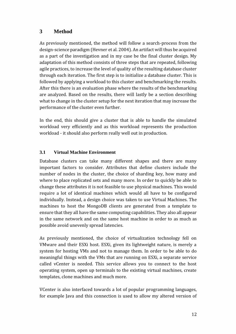
Figure 3.1: Machine hierarchy on main virtual machine host
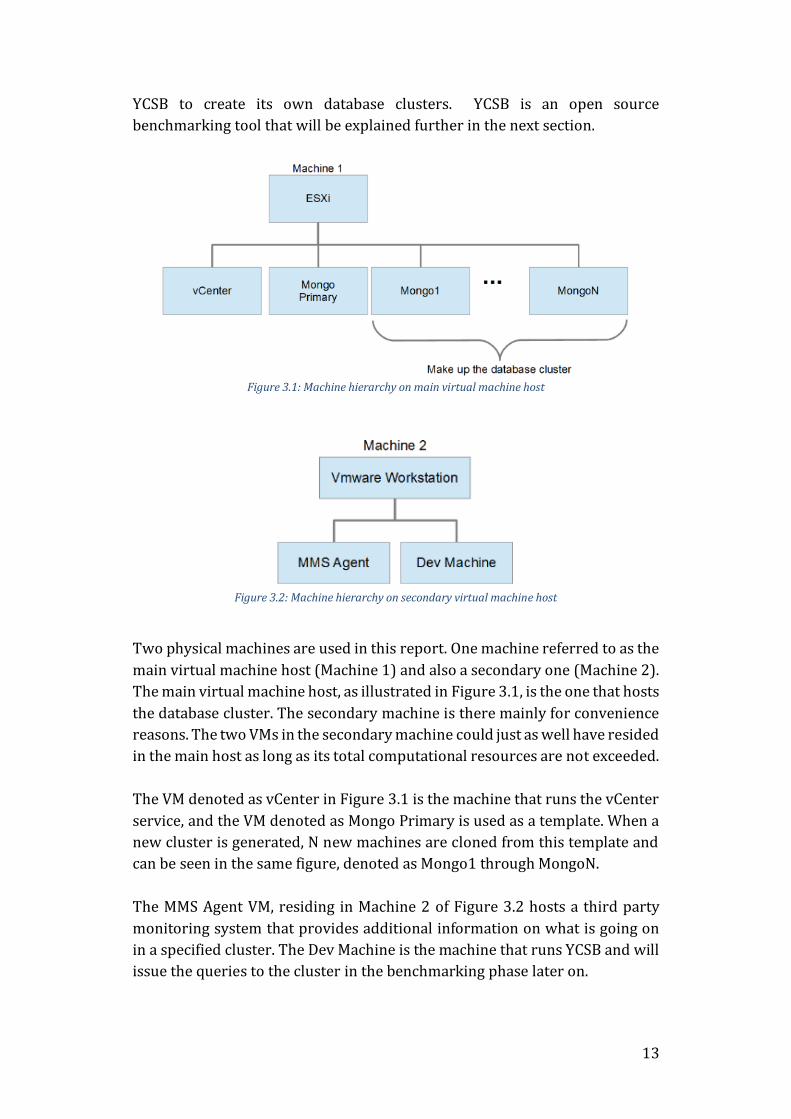
Figure 3.2: Machine hierarchy on secondary virtual machine host
Two physical machines are used in this report. One machine referred to as the
main virtual machine host (Machine 1) and also a secondary one (Machine 2).
The main virtual machine host, as illustrated in Figure 3.1, is the one that hosts
the database cluster. The secondary machine is there mainly for convenience
reasons. The two VMs in the secondary machine could just as well have resided
in the main host as long as its total computational resources are not exceeded.
The VM denoted as vCenter in Figure 3.1 is the machine that runs the vCenter
service, and the VM denoted as Mongo Primary is used as a template. When a
new cluster is generated, N new machines are cloned from this template and
can be seen in the same figure, denoted as Mongo1 through MongoN.
The MMS Agent VM, residing in Machine 2 of Figure 3.2 hosts a third party
monitoring system that provides additional information on what is going on
in a specified cluster. The Dev Machine is the machine that runs YCSB and will
issue the queries to the cluster in the benchmarking phase later on.
14
3.2 Benchmarking Tool
The benchmarking of a database is done in two steps. The first constitutes
filling a collection up with some initial data. After this is done, a workload is
applied. This workload will be explained more thoroughly in the next section
but simply put, it is a set of queries to the database which are executed in the
same fashion as a stress test. The queries are fed to the database as quickly as
possible and the number of queries that the database is able to handle is then
measured.
Yahoo! Cloud Serving Benchmark (YCSB) is an open source tool, developed by
Yahoo! to do exactly this. It is written in Java and contains libraries, both for
generating your own generic workloads and applying these workloads to a
database (Kashyap et al. 2013). The workloads are generic in the sense that
they are not database specific, you do not need to take the choice of DBMS into
consideration at all when defining the workload. It is built upon the fact that
all interaction with the DBMS by the workload will be through simple queries.
These simple queries are inserts, updates, deletes and scans. Each operation
against the DBMS is randomly chosen between these four operations, however
the distribution between them is set by the user (Cooper et al. 2010).
An abstract class of these basic queries is given for the user to interface the
tool towards whatever DBMS is being used, in my case MongoDB. Now it is
possible for YCSB to apply my workload to my database. While doing this,
YCSB collects valuable statistics of how well the database is performing to the
workload. The metrics are for instance the number of operations per second,
average overall latency and average latency for different types of queries.
In addition to writing my own workload and database interface I have made
some additions to this tool. As I am working with ESXi and vCenter, I have
made my own solution for automatically generating database clusters.
VCenter is interfaced towards Java. I use this in order to let my YCSB instance
automatically create the set of virtual machines needed to check the
performance of some cluster design. The characteristics of the cluster is
defined in an XML configuration file that the altered YCSB parses and then uses
to create a new database cluster using only new virtual machines. The virtual
machines are all created from the same template to ensure identical hardware
capabilities. SSH connections are then set up to these VMs to make them into
a working MongoDB cluster with properties also defined in the configuration
file.
15
All in all, these additions make YCSB not only able to benchmark existing
databases, but also to be able to easily experiment with new and different
cluster setups and compare the results between them.
Furthermore - Cooper et al. (2010) writes about measuring elasticity, the
ability to adapt to new nodes in the cluster, and how this can be measured by
YCSB. I have added functionality for YCSB itself to be able to modify the
number of nodes in a cluster and therefore not have the measurements being
reliant on external interactions. Elasticity is however not something that plays
a big part in this report.
3.3 Workload
YCSB contains libraries for generating your own workload. The workload is
built to replicate the Radish collection of storing users. A method for
generating random users that follow the same schemas with the same fields
as the production environment was developed. In the first phase of the
workload where the collection is filled up with entries, 50 000 of these random
users are generated and entered. As we will see shortly, most of the operations
in the benchmarking phase are reads, therefore it is necessary that the
collection is not empty when the benchmarking starts and it can also be good
to warm up the CPU cache and pipelines (Lungu et al. 2013). The number 50
000 was chosen as it is a sufficiently large dataset for MongoDB to divide the
collection into several chunks and therefore initiate the MongoDB load
balancing algorithm. A chunk is defined as the smallest amount of data that
can be moved in one load to achieve balance between the shards. Another way
of describing it is by saying that each shard consist of one or more chunks.
MongoDB takes care of moving data between shards in a cluster but it does not
trigger unless the data reaches a certain size. It is also not so large that it
exceeds the RAM capacities of the VMs which would be a very large bottleneck
for the performance of the cluster.
The next phase consists of a series of operations to the database, executed by
a maximum of 40 worker threads by an arbitrary amount of CPU cores. These
operations are the previously mentioned inserts, updates, reads and scans.
Each thread chooses one of these operations at random but with different
distributions. The distributions are chosen as replicas of the current
production environment and the accumulated statistics from the live machine
was taken and normalized.
16
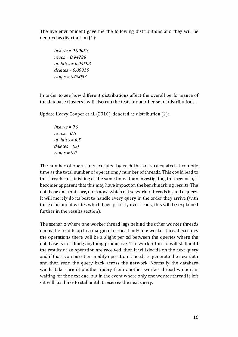
The live environment gave me the following distributions and they will be
denoted as distribution (1):
inserts = 0.00053
reads = 0.94286
updates = 0.05593
deletes = 0.00016
range = 0.00052
In order to see how different distributions affect the overall performance of
the database clusters I will also run the tests for another set of distributions.
Update Heavy Cooper et al. (2010), denoted as distribution (2):
inserts = 0.0
reads = 0.5
updates = 0.5
deletes = 0.0
range = 0.0
The number of operations executed by each thread is calculated at compile
time as the total number of operations / number of threads. This could lead to
the threads not finishing at the same time. Upon investigating this scenario, it
becomes apparent that this may have impact on the benchmarking results. The
database does not care, nor know, which of the worker threads issued a query.
It will merely do its best to handle every query in the order they arrive (with
the exclusion of writes which have priority over reads, this will be explained
further in the results section).
The scenario where one worker thread lags behind the other worker threads
opens the results up to a margin of error. If only one worker thread executes
the operations there will be a slight period between the queries where the
database is not doing anything productive. The worker thread will stall until
the results of an operation are received, then it will decide on the next query
and if that is an insert or modify operation it needs to generate the new data
and then send the query back across the network. Normally the database
would take care of another query from another worker thread while it is
waiting for the next one, but in the event where only one worker thread is left
- it will just have to stall until it receives the next query.

17
This will definitely compromise the results and this needs to be taken into
consideration when evaluating the results as the ops/sec might not be correct
near the end of executing a workload.
A potential workaround of this would be to have a static, volatile counter for
the worker threads to keep track of the total number of operations.
Continuously flushing increments and synchronizing this counter with RAM
for the different threads instead of the local cache might also influence the
results though, as it could potentially stall all worker threads while an update
to the counter variable is being flushed.
A total of 250 000 operations are executed by the worker threads in this
fashion.
3.3.1 Social Networking Illusion
As we can see from the previous section, a vast majority of the operations used
in the production environment are reads. YCSB’s default behavior is to store
the IDs of elements added to the database and uniformly choose one of them
for each read. This would lead to the contents of the datastore being accessed
uniformly and when considering possible usage scenarios and the resulting
flow of data you realize that this most likely is not the case.
The datastore will store data on users and users’ photos. A more likely usage
scenario is that a person is more likely to check out information on people in
his or her friend circuit than any arbitrary person in the system. In technical
terms this means that the application is more likely to query the database on
a predefined subset of its data rather than any uniformly chosen entry given a
previous entry. I want the workload to take this into consideration as it might
affect the result of the benchmarking.
In order to accomplish this, I need to generate a social network. There are
many factors to take into consideration when designing these social networks.
For instance there is the phenomenon referred to as the “small-world
problem”. Stanley Milgram (1967) describes it very elegantly by considering
two persons X and Z that do not know each other. They might however still
share a mutual acquaintance, e.g. a third person Y that knows both X and Z. By
then thinking of a chain of acquaintances where X knows Y and Y knows Z. It
has been suggested that the entire world's population can be connected in this
way by using only six acquaintances in the chain (Newman et al. 1999). You
also have something called hubs or clusters where within a small locale there
are a lot of individuals who all know each other. These are brought on by the
fact that social networks have the behavior that if person A knows person B
and person B knows person C, it is more likely that A knows C than it would be
18
if A and C were just two random people in the universe (Newman et al. 1999).
A networks likelihood to contain these hubs is referred to as the clustering
coefficient (Prettejohn, 2011). If a network has a high clustering coefficient it
is referred to as scale-free. This means that the network will grow through its
hubs and also means that the number of connections between nodes that are
not hubs is not likely to change even if the network rapidly increases in size.
An example could be the World Wide Web, or international airline traffic.
These are scale-free networks that are held together by hubs in the shape of
very large websites and major airports.
An algorithm exists for generating such a network that has the properties of
scale-free and small-world, created by Klemm and Eguílez (Prettejohn, 2011).
As previously mentioned, the benchmarking is conducted in two steps. Firstly
the collection is filled up with content and for this example I choose the user
collection. After the users have been entered, the algorithm by Klemm and
Eguílez is applied to generate a social network from these users where each
user is considered a node and some nodes are considered hubs. When the
second phase of the benchmarking starts, each worker thread that will query
the database chooses a starting node in the social network at random. From
this starting node, it is easy to fetch the subset of the users which are
considered acquaintances of the current node. The next query executed by the
worker thread will, with high probability, be for one of the nodes in this subset
and this pattern is repeated throughout the lifecycle of the worker thread.
19
4 Result
In this section, the method described in the previous section will be
demonstrated in a practical example where the collection of users in our
predefined use case is subject for optimization.
The results are primarily going to be focused on the number of operations per
second that can be handled by the database or database cluster. The process
of getting these numbers will be conducted in a pattern where I first explain
the database setup that will be benchmarked, and this is followed by an
analysis where a corrective action will be given. The corrective action will be
focused on the results of the setup of the current iteration and how the setup
can be changed in order to improve these results. The changes will be applied
to the next setup and the process starts all over again. This process is tightly
linked to a core aspect of agile methodology where the main focus is on getting
the software up and running. Once it is running, improvements are made
through an iterative process (Turk et al. 2002).
As mentioned, the results will be focused on the number of operations per
second handled by the database. This will however fluctuate somewhat even
when applying the workload to two identical database setups. This is due to
many factors, but the two major ones are the randomness of the workload and
the unpredictability of the host operating systems. The workload decides
which type of query to ask the database at random, however the distribution
is not uniform. This randomness makes two runs unlikely to be identical,
particularly as writes to the database gets priority over reads (The MongoDB
2.4 Manual, 2014). This causes chain effects that affect all threads issuing
queries and the results will therefore fluctuate to some extent. The host
operating system also plays a big part as there are large uncertainties when
operating system features are run and use up computing resources.
Following this uncertainty, the tests were run multiple times and the average
performance is the one I put main focus on. The average performance is
calculated by using a confidence interval. This is a common tool in statistics
and allows us to say something about the averages of large data sets using a
limited amount of sample values.
A confidence interval is defined as a number range that with some certainty
contains the actual average given from a limited number of samples. The limits
to the number range are calculated as:
𝐿𝑜𝑤𝑒𝑟 𝐿𝑖𝑚𝑖𝑡 = 𝑀 −𝑡∗𝜎
√𝑛
𝑈𝑝𝑝𝑒𝑟 𝐿𝑖𝑚𝑖𝑡 = 𝑀 +𝑡∗𝜎
√𝑛

20
Where M is the sample average, σ is the standard deviation which in turns is
the square root of the sample variance, t is tied to the confidence level and n is
the number of sample values. We see that the size of the interval decreases as
n grows larger which is intuitive as more samples should give us a better
reading on the actual average.
For this report, the sample values used in the confidence interval is the
average number of ops/sec for each run. The confidence level used is 95%
(which gives us a t=1.96) and sample values are assumed to follow a normal
distribution. Each run gives a new sample value, representing of the average
number of operations for that run. From the definition of the confidence
interval we can see that the interval decreases in size with larger sample sizes.
The tests were run until the size of the confidence interval was at most 4% of
the size of the sample average, with two exceptions.
All virtual machines used in the experiment are identical and have the
hardware capabilities of 1500 MHz worth of computing power, 1024MB of
RAM memory and 90GB of storage. The operating system in use is Ubuntu
12.04 LTS and the MongoDB version is v2.4.10.
For almost every different database setup, two different versions of the
workload will be applied. These two follow the same basic procedures but the
distributions between the different types of operations towards the database
are changed to see if this has any major impacts on the performance.
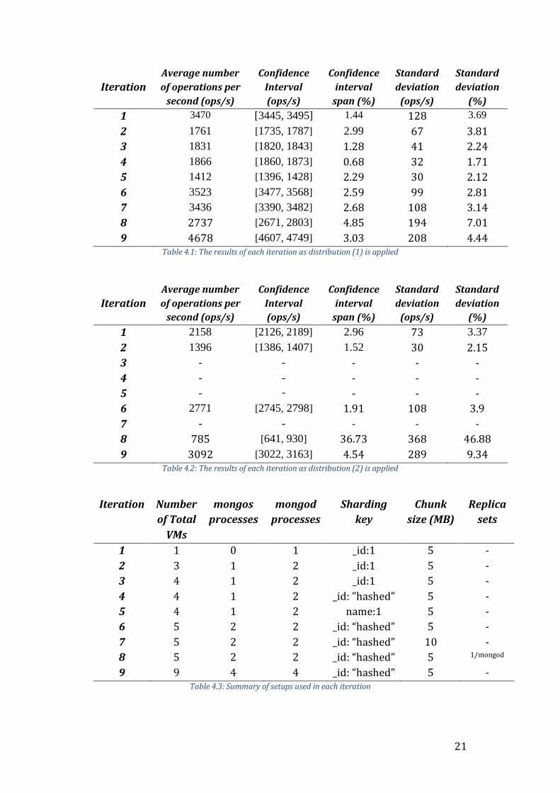
Below are three tables, Table 4.1 and Table 4.2 will be the main subjects of the
analysis of each iteration whilst Table 4.3 contains a quick summary of the
setups used in each iteration.
21
Iteration
Average number
of operations per
second (ops/s)
Confidence
Interval
(ops/s)
Confidence
interval
span (%)
Standard
deviation
(ops/s)
Standard
deviation
(%)
1 3470 [3445, 3495] 1.44 128 3.69
2 1761 [1735, 1787] 2.99 67 3.81
3 1831 [1820, 1843] 1.28 41 2.24
4 1866 [1860, 1873] 0.68 32 1.71
5 1412 [1396, 1428] 2.29 30 2.12
6 3523 [3477, 3568] 2.59 99 2.81
7 3436 [3390, 3482] 2.68 108 3.14
8 2737 [2671, 2803] 4.85 194 7.01
9 4678 [4607, 4749] 3.03 208 4.44 Table 4.1: The results of each iteration as distribution (1) is applied
Iteration
Average number
of operations per
second (ops/s)
Confidence
Interval
(ops/s)
Confidence
interval
span (%)
Standard
deviation
(ops/s)
Standard
deviation
(%)
1 2158 [2126, 2189] 2.96 73 3.37
2 1396 [1386, 1407] 1.52 30 2.15
3 - - - - -
4 - - - - -
5 - - - - -
6 2771 [2745, 2798] 1.91 108 3.9
7 - - - - -
8 785 [641, 930] 36.73 368 46.88
9 3092 [3022, 3163] 4.54 289 9.34 Table 4.2: The results of each iteration as distribution (2) is applied
Iteration Number
of Total
VMs
mongos
processes
mongod
processes
Sharding
key
Chunk
size (MB)
Replica
sets
1 1 0 1 _id:1 5 -
2 3 1 2 _id:1 5 -
3 4 1 2 _id:1 5 -
4 4 1 2 _id: ”hashed” 5 -
5 4 1 2 name:1 5 -
6 5 2 2 _id: “hashed” 5 -
7 5 2 2 _id: “hashed” 10 -
8 5 2 2 _id: “hashed” 5 1/mongod
9 9 4 4 _id: “hashed” 5 - Table 4.3: Summary of setups used in each iteration
22
4.1 Iteration 1
Setup
The first setup is the simplest of all possible setups - a singleton solution where
only one VM runs the MongoDB client without changing any of the MongoDB
settings.
Analysis
The value of most interest here is the 3470 ops/s as can be seen from table 4.1.
We get this value through running the benchmarking with distribution (1).
This does not tell us much at this moment but it is a good reference point for
other setups later on. It should be noted that this is the sample average.
However enough samples were taken to provide a 95% confidence level of the
actual average being within [3445, 3495] operations per second.
There are also two graph of the CPU activities of the VMs during the course of
a few of the runs that can be seen in Appendix A, Results 4.1 as Figure 4.1.1
and Figure 4.1.2. The pattern is quite clear, a small initial spike in activity when
the database is being filled up with content, then some idle time and finally
followed by a longer spike where the benchmarking phase is running. This
pattern is repeated over and over again.
It is worth noting that there are a few data points on the graphs that suggest
that the CPU activity exceeded its limit of 1500 MHz. I interpret this to be an
inaccuracy of the graph sampling tool. The data points for this graph are
generated by sampling the CPU activity and this is only done once every 20
seconds. VMware Inc. (2013) ensures us that limits on CPU resources are met,
but not in which time spectrum they are met. It is therefore natural that for a
very short interval, a machine might be slightly exceeding its CPU limit.
Something else that is worth noting is that the setup performs considerably
worse in distribution (2) than it does in distribution (1). This is however
anticipated as more updates to the database means more locks, as writes to
the database gets priority over reads.
Naturally a lot of things can be done in this stage to improve the performance
as the setup is a singleton solution with complete default settings. In order to
see how our choices affect the performance however, it is in our best interest
to only perform one larger modification at the time. The focus of this report is
database clusters, so for the next iteration, the singleton solution shall be made
into a cluster.
23
4.2 Iteration 2
Setup
For this iteration, we shall be using a cluster setup. The cluster consists of
three virtual machines denoted vmMongos, vm2 and vm3. Clusters in
MongoDB have a few requirements in order for them to work. You need a
mongos instance or query router as it is also called. This is a lightweight
process that acts as an interface between the cluster and the outside world
(The MongoDB 2.4 Manual, 2014). The queries go through mongos and are
redirected to the right machine in the cluster. You also need shards, a shard in
a cluster is MongoDBs name for a computing resource and is implemented as
a mongod process. Theoretically a single machine can host an arbitrary
number of mongod and mongos processes, although its computing resources
of course remain the same. Throughout the rest of this report, each virtual
machine will host a maximum of one mongod or mongos process unless
otherwise specified.
A cluster can have an arbitrary number of shards and mongos instances. You
also need three config servers. These are processes that store metadata of the
cluster, three are required in order to create the necessary redundancy as the
config server would otherwise act as a single point of failure for the cluster.
In this iteration, vmMongos acts as the query router of the cluster while vm2
and vm3 are added to the cluster as shards. The config servers are all running
on vmMongos.
In order for MongoDB to know how to spread the data across the shards, a
sharding key must be provided. The choice of sharding key here fell on using
the _id field. This is a default field which always exists for any given entry in
MongoDB and if it is not specified by the user, MongoDB will automatically
generate it. As previously mentioned, there are several ways of using a field as
sharding key and in this setup, a range-based distribution was chosen.

24
Analysis
The value of most interest here is the 1761 ops/s from running distribution
(1) as can be seen from Table 4.1. This result is quite surprising as the cluster
with three times the hardware capabilities actually performs worse than the
singleton solution. From examining the CPU activities of the different
machines in Figures 4.2.* it is noticeable that neither vm2 nor vm3 are
working at their maximum capacity whilst vm1 seems to be a bottleneck.
Vm1 hosts the mongos process that redirects queries to the cluster to the
correct shard. This process is supposed to be lightweight and not require any
extensive resources so this is very unexpected behavior. VmMongos also hosts
the config servers which are tracking the metadata of the cluster. In order to
see if these config servers uses up a lot of resources, a new VM will be
introduced to host these in the next iteration.
25
4.3 Iteration 3
Setup
In order to investigate what is consuming the CPU resources of vmMongos, a
choice was made to move the config servers to a separate virtual machine and
rerun the same test as Iteration 2. The new VM will be denoted as vmConfig.
Analysis
Upon examining the CPU utilizations of Figure 4.3.* it is once again very
obvious that the CPU resources of vmMongos is the clear bottleneck of the
cluster performance. From inspecting the CPU consumption of vmConfig it is
also clear that the config servers did not consume a lot of resources which
explains why the performance increase in ops/s was very minimal in
comparison to Iteration 2.
Inspecting the processes during the course of a run also revealed that it is
indeed the mongos process that is using a vast majority of the computing
resources. In an attempt to understand what is going on, the sharding key will
in the next iteration be changed from being range-based to being a hashed
value on the _id field.

26
4.4 Iteration 4
Setup
For this iteration, one change was made and that was the choice of sharding
key. Instead of arranging elements in an ascending order on the value of the
_id field, a hash value is computed from this value. The desired outcome here
is that the entries should be spread out more evenly amongst the shards and
that the mongos process should more easily be able to locate where an
element resides than before when all elements had to be sorted.
Analysis
As we can see in Table 4.1 and 4.2, the results were yet again a slight
improvement. However the CPU resources of vm1 remains the big bottleneck
as can be seen in Figure 4.4.*.
Not a lot of information can be extracted of exactly what is going on in the
mongos process. The description of the process is that it just reroutes queries
from the application to the correct shard or shards (The MongoDB 2.4 Manual,
2014). This process is highly dependent on the sharding key so in order to
resolve this problem, yet another different sharding key will be chosen for the
next iteration.

27
4.5 Iteration 5
Setup
The setup is once again very similar to that of the previous iteration only in
this one, the name field is chosen as sharding key instead of the _id field. The
sharding is range-based.
Analysis
As can be seen from Table 4.1, this time there was a drastic decrease in
performance after only changing the sharding key. This is because YCSB
queries elements by their _id. Since we shard the cluster based on the name
field, it is impossible for the mongos process to reroute the query to only one
shard and it has to do a broadcast amongst shards to find out where the
element is stored. This overhead gives rise to the decrease in performance
compared to when the cluster was sharded on the _id field.
This insight has a big impact on designing this cluster. It greatly limits our
choice of sharding key as the mongos process is already the bottleneck of our
cluster. Any sharding key where the _id field is not present will cause an extra
overhead to the mongos process and bring down the performance even more.
It is possible to tweak the sharding key that uses the _id field even further for
a potential increase in performance but it is highly unlikely that it will be
enough for the mongos not to be a bottleneck.
We do not want the mongos process to be a bottleneck, primarily for two
reasons. The first one is because it does not really store any persistent data
and is bound by the CPU resources of the host machine. Assigning more CPU
resources to the machine that runs the mongos will greatly increase the
throughput. The second reason is that it is easy, and common practice, to add
several mongos instances to a cluster. One can then, on the application level,
just choose one of these mongos instances at random to increase the
throughput of the mongos instances to the mongod instances where the data
is stored.
The results so far insinuate that the mongos instance is likely to always be the
bottleneck of the cluster performance with the current hardware
specifications. The next step in developing this database must therefore be to
add an extra mongos instance to the cluster.
It should be noted that the mongos process can be hosted on the same virtual
machine as the ones that are running mongod and acting as shards. However

28
for the sake of more easily being able to interpret the results - an entirely new
virtual machine will be used.

29
4.6 Iteration 6
Setup
For this setup, the sharding key is once again set to the hash of the _id field.
Two VMs denoted as vm1 and vm2 are used to host one shard each and two
additional machines denoted as vmS1 and vmS2 are used to host a mongos
instance each. Upon issuing a query to the cluster, the benchmarking tool will
choose one of these mongos instances at random to send the query to.
Additionally there is a separate VM for the config server similarly to previous
iterations.
Analysis
As can be seen from the Figure 4.6.*, the activity of both vm1 and vm2 is now
much higher for both distributions. This is very expected as the throughput is
almost twice as high as it was in Iteration 4 when the same setup was used but
with only one mongos instance as can be seen from Table 4.1 and Table 4.2.
These results suggest that the performance might be improved even further
through adding yet another mongos instance as they are still currently the
bottleneck.
There is however another thing we can do that might optimize the existing
mongos instances even further and enough for them not to be the bottleneck
– changing the chunk size of the cluster. As previously mentioned, mongos
divides data in a collection into shards by some shard key. This is achieved by
dividing the data into small pieces referred to as chunks. These chunks are
then spread evenly across the shards to form a pseudo balanced distribution
of the elements. After this is done, a balancing algorithm runs in the
background of the mongos machines and makes sure that the balance between
shards is kept. The balance might be compromised as new inserts might not
be evenly distributed amongst the shards and we may also change the value of
the field that is used as sharding key, causing it to migrate to another chunk on
another shard.
Given that the CPU load of vm1 and vm2 are fairly even which we saw from
Figure 4.6.*, it is a fair assumption that the elements are spread between the
two shards in a good way. However what we do not know is if the mongos
instances are doing a lot of unnecessary balancing work because our chunks
are too small.
One can consider the two extreme cases of the chunk size. If we chose a
minimal chunk size, the elements would be balanced individually and each
update or insert would lead to elements being rearranged by the balancer to

30
achieve a perfect distribution. The other extreme case is when the chunk size
is chosen to be way too big and we do not achieve any balance between the
shards at all as all elements fit in one chunk.
Since our distribution right now seems fairly good, there might be room to
increase the chunk size even further and still keep a good enough level of
balance but demand less work from the balancer process. This is what will be
tried out in the next Iteration.
31
4.7 Iteration 7
Setup
As explained in the analysis of Iteration 6, there is some potential to optimize
the cluster further through altering the chunk size. This setup is identical to
that of Iteration 6 with the modification that the chunk size has been doubled
from 5MB to 10MB.
Analysis
The CPU graphs of this Iteration were left out as they did not reveal anything
important. Distribution (2) was also not run as it was obvious from running
distribution (1) that we did not achieve the desired outcome and this can be
seen in Table 4.1. The larger chunk size gave us the anticipated effect that the
elements would be less balanced than before. However, the results also reveal
that the gain that we get from the balancer not having to work as hard is not
weighing up for this imbalance.
It seems now that it is very hard to do any major changes that might have a
good impact on the performance. This is true both for the mongod instances
and the mongos instances. The mongod instances are doing the absolute
minimal work required as they are continuously getting lookups on the _id
field that we have an index for and the elements are evenly distributed across
the shards. The mongos instances are also very hard to optimize as we have
already eliminated broadcast occurrences by dividing the data by the _id field
which is a field involved in the query to the cluster. The job of creating the hash
values for elements and figuring out in which shard they belong could be made
more optimized through using a range-based sharding key on the same field.
This is true as this would only require a simple comparison by the mongos
instances to decide where an element belongs. Although, we have already
shown that the hash-based sharding key outperforms the range-based
sharding key overall as the overhead of keeping the elements ordered is higher
than the overhead of computing the hash value.
It is important to point out that the real scenario will most likely have a larger
variety of queries but unfortunately that data was not available at this time.
At this point, the major performance enhancers apart from adding more
computing resources have been explored and instead I choose to focus the
next iteration on the availability of the cluster. I will increase the availability
by adding redundancy to the mongod in the shape of replica sets. The mongos
instances are already redundant as the cluster merely needs one of these to
function.
32
4.8 Iteration 8
Setup
For this iteration, the setup will follow that of Iteration 6. The cluster will have
two mongod instances and two mongos instances, each on a separate VM and
then an additional VM to host the config servers. The sharding key will be the
hash of the _id field of the elements and the chunk size will go back to 5MB as
iteration 7 showed that the increase did not positively affect the performance.
The mongod instances will however be slightly different to that of Iteration 6.
I will increase the availability of the cluster by adding redundancy to the data
and the computing resources. MongoDB’s way of doing this is through the use
of replica sets. This is a way of connecting two or more mongod instances that
may be running on separate machines. One of these mongod instances will be
referred to as the Primary and its data will be propagated to all the other
mongod instances, referred to as Secondary, in the replica set.
Once this is done, all mongod instances in the replica sets will mirror each
other’s data. Changes to the data in one mongod instance will eventually
propagate to the other mongod instance. An eventually consistent level of
atomicity is used here as a mongod instance cannot acquire locks on other
mongod instances.
It is important to point out that unless otherwise specified in the
configurations of the mongos instances or a specific mongod instance is
directly queried – queries will always go to the Primary mongod instance as
long as this is available. If the Primary would become unavailable, an arbiter
will elect one of the Secondary’s as the new Primary.
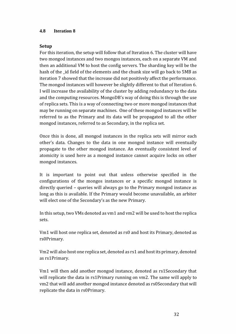
In this setup, two VMs denoted as vm1 and vm2 will be used to host the replica
sets.
Vm1 will host one replica set, denoted as rs0 and host its Primary, denoted as
rs0Primary.
Vm2 will also host one replica set, denoted as rs1 and host its primary, denoted
as rs1Primary.
Vm1 will then add another mongod instance, denoted as rs1Secondary that
will replicate the data in rs1Primary running on vm2. The same will apply to
vm2 that will add another mongod instance denoted as rs0Secondary that will
replicate the data in rs0Primary.
33
What this means is that in this case, all data will be stored twice and both vm1
and vm2 will host the entire dataset. Queries however will only be directed
towards one of the VMs at the time as they will always be directed towards the
Primary of each replica set.
The overhead associated with this is that we require twice as much storage
capacity to store our data and each VM will need to spend some of its
computing resources on propagating changes between Primary and
Secondaries.
Figure 4.8: Visualization of replication
Analysis
The CPU charts were once again left out as they did not reveal anything
interesting. As the setup of this iteration is very similar to that of Iteration 6, it
is of interest to see how the replicated sets affected the performance.
For distribution (1) the results are quite anticipated. As we can see from Table
4.1, the throughput went from 3523 ops/s to 2737 ops/s and a decrease in
performance was expected due to the overhead associated with replica sets.
Notable is also that the standard deviation is considerably higher than in
previous iterations.
As for distribution (2) we see a dramatic decrease in performance as it went
from 2771 ops/s to 785 ops/s as specified in Table 4.2. The lowest recorded
run only averaged 233 ops/s and the standard deviation is by far the largest
yet.
These results can be explained as they are very tied to the distributions
between different operations. Reads require no changes to be propagated
between Primary and Secondary instances whilst updates & inserts both
acquire locks and require the changes to be applied to the Secondary set. In
Distribution(1), a vast majority of the types of operations were reads which in
theory would not lead to any decrease in performance at all which is why the
overall performance managed to stay up quite well. In distribution (2)
however we specify that 50% of the operations towards the database should
be updates. This is why we see this massive decrease in performance and upon
34
inspecting the database lock times, they are also much higher than before. The
lock times are a big factor to why we see the rapid increase in standard
deviation. Locks have a tendency to cluster, particularly when we have many
update operations as they are much slower than reads and also have priority
over reads. This leads to the database being locked to reads for long periods at
a time and the update operations being executed only one at a time, resulting
in very bad performance with large fluctuations.
This is something that must be taken into consideration when adding replica
sets as they have a potential of stealing a lot of computing resources from their
hosts.
In the next, and last iteration, the setup from Iteration 6, which is the cluster
with best throughput and performance so far, will be scaled up to twice its
previous size in terms of VMs. This will be done in order to investigate how its
size affects the throughput and make sure the setup is able to scale well when
more computing resources are added.
35
4.9 Iteration 9
Setup
In this iteration, the setup from Iteration 6 will be reused to a large extent but
with 4 extra VMs. Two of these extra VMs will serve as shards, running their
own mongod instance. The other two will act as mongos instances.
Analysis
The CPU plots were once again left out as they did not reveal anything
interesting. All VMs except the one running the config servers operated at
maximum capacity all throughout the tests. It can be seen from the results in
Table 4.1 and Table 4.2 that we did achieve an increase in performance by
adding more computing resources. How well these new resources affected the
performance does however fluctuate quite significantly based on the
distribution between elements that is currently being used.
For distribution (1) we saw the throughput go from 3523 ops/s to 4678 ops/s
as we doubled the number of shards and mongos instances. At first glance, a
100% increase in throughput might have been the expected increase here as
we double the amount of computing resources. This could be possible if all of
the operations to the database would be reads. Reads can be parallelized and
as we have spread out the elements fairly well by using a hash value, we had
also spread out the work of fetching the elements evenly across the shards and
potentially resulting in a linear increase in throughput.
Regarding updates, inserts and scans this not the case. Updates and inserts will
eventually trigger the balancer to start moving chunks around between shards
in the cluster and thus stealing computing resources. As the elements are
distributed on a hash value and appear quite randomly across the shards, it is
very unlikely that a scan will only target one shard in the cluster. This means
that the throughput of scans may actually suffer from adding more shards.
This problem with scans can be circumvented by use of a range-based
sharding key but as we saw from iteration 4, the increased performance for
scans was not enough to compensate for the performance decrease in the
other operations.
In distribution (2) the increase in performance was significantly smaller than
in distribution (1). This is due to the fact that we have such a high portion of
update operations. As previously mentioned, the update operation does not
scale as well through using sharding and that is manifesting itself here.
36
5 Delimitations & Problems
For simplicity I chose to divide the project into three separate parts and talk
about the delimitations and problems related to each part individually. One
part is the method in which the project is conducted. Another which is about
the technical problems of the tools involved and finally a part which talks
about possible delimitations when applying the tools and methods to the use
case of Radish.
5.1 Method
The purpose of this project is to be able to fine tune databases into performing
as optimal as possible. We have already seen the importance of the workload
and the different distributions of operations and the major impact these have
on the results.
It is important that the simulated workload replicates the actual production
environment as well as possible. If it does not, we are essentially optimizing
the database for circumstances that will not be the same ones as it will face in
production.
Furthermore it is also common to have to make adjustments to databases
during the life cycle of a project in order to accommodate new features and so
on. These adjustments may influence the usage pattern of the database and
lead to the optimal setup being somewhat shifted. In this scenario, the changes
must be applied to the workload and tests reran in order to establish the new
optimal cluster setup.
Lastly there is no way of knowing if an optimal setup has been achieved. The
method and tools provide ways of comparing two setups against each other
but it is up to the person conducting the testing to decide when an acceptable
setup has been discovered.
5.2 Technical
For this project, a variety of tools were used and each of them have their own
set of delimitations and problems. A major part of the project has been the use
of the open source tool YCSB. YCSB has several limitations and one is that it is
only possible to run the simulations on one machine at a time and that machine
may only have a maximum of 40 threads. As it is developed in Java there is no
support for setting the affinity of threads and this may compromise the results.
If you are benchmarking a very large and fast cluster, it may actually be YCSB
that acts as a bottle neck.
37
To host the virtual machines VMware ESXi was used. Tests have been
conducted to prove its fairness and efficiency when dividing computing
resources (VMware Inc, 2013). However as the machines computing power is
bound by the computing power of its host, clusters of sizes larger than 9
machines could not be explored in this project.
Finally, different chunk sizes were explored in the results section of this
report. The imbalance between how many elements resided on each shard
caused by this lead to a decrease in performance and the modification was
abandoned. The optimal chunk size is very much relative to the dataset in
question. The larger the dataset is, the more resilient it becomes to larger
chunk sizes and these larger chunks will not cause as large of an imbalance. As
the datasets tend to grow over time, there will most likely be a threshold
sometime in the future when there will be a performance gain by increasing
the chunk size. This was however not explored as a dataset of static size was
used.
5.3 Current Use Case
The result section is primarily focused on how to develop the best possible
cluster setup for the use case of Radish. To do this, the workload was built to
replicate the production environment that Radish is undergoing as well as
possible. However, specific data on the type of queries used was not available
at this time so the default behavior of YCSB was used instead, which is to query
elements based on their _id field. Furthermore, the database schema has
undergone big changes since this project started and there is a delimitation in
place to develop the cluster as well as possible under the circumstances that
existed at the time when the basis of the project was established.
Another delimitation that was put in place in relation to this use case was the
use of datasets that did not exceed the RAM capacity of the VMs. As the desired
outcome was a cluster with as high throughput as possible, it was a natural
choice to not store more data on each machine than the capacity of its RAM
memory. The use of larger datasets would have led to other complications too
as the VMs run on the same disk of its host and would have potentially
compromised each other’s read/write capacities.
38
6 Discussion
6.1 Related Work
The scientific body of this study can be divided into two parts. One in which the benchmarking of databases is explored and another where we explore strategies for designing database clusters as well as optimizing these designs. Benchmarking databases has been going on for quite some time. Rubenstein et al. established a method for benchmarking databases based on querying data with a set of simple database operations already in 1987. These were done for relational databases however, but the principles extend also into the world of document stores (Cattell, 2010). Throughout the years, multiple experiments and comparisons have been carried out on these document stores where they are both compared to each other and relational databases (Cooper et al. 2010) (Cattell, 2010) (Kashyap et al. 2013). Even though the methods and tools for acquiring the benchmarks have been perfected over the years and some of the previous research deal with DBMSs with cluster support (Cattell, 2010), very little emphasis has been put on measuring the performance of the cluster setups. The effort has instead been on deciding which DBMS can handle a given workload the best in a singleton setting and perfecting the benchmarks to measure this (Cattell, 2010. What this study has now established in the area of benchmarking, is a way of measuring the performance for clustered solutions rather than just single nodes. It has also been shown how these insights about how the cluster setups affect the performance can be used to gradually improve the performance of an existing database cluster through altering the cluster configuration. Furthermore it has also been shown how a benchmarking workload can look in the case of a social networking application and how these can be generated through using the Klemm and Eguilez network creation algorithm (Prettejohn, 2011). It has been discussed that whilst there are indeed best practices one can follow when designing datastores in the SQL world (Harrington, 2002) (Stonebraker and Cattell, 2010), very little research exist about how one should design database clusters for document stores. Best practices for document stores are very hard to find by due to the case specific nature of these datastores (Chodorow, 2011). There are however a lot of documentation and guides for how features of document stores can be used to someones advantage when designing a database cluster, particularly for the MongoDB datastore (The MongoDB 2.4 Manual, 2014) (Chodorow, 2011). However little to no research exist around establishing what effect these features may have on a clustered solution as a whole. The existing research and documentation also covers different configuration settings and how they could potentially be used to someone’s advantage when designing a database cluster. How these features and settings fit into a particular context however

39
is for the designer of the database cluster to figure out. This is in some cases a guess work and of course makes it very tricky to design the best possible database cluster. This study is able to extend the existing body of knowledge through providing a way of verifying whether using some feature or configuration change achieves the desired effect in someone’s specific context. The method for designing database clusters provided in this study makes the effect of changes much more tangible. This is due to the fact that the performance of a design can be quantifiable and measured towards other designs as well as modified without affecting the live production data. It has also been shown that performance wise, the advantages of going from a singleton solution to a cluster don’t actually outweigh the overhead until the cluster reaches a sufficient size. 6.2 Ethical Considerations
This study about optimization of database cluster performance contains no obvious ethical concerns. However, when considering the product that this particular scenario is addressing, one can recognize some ethical concerns regarding the potentially sensitive information that is handled. As MeBox is accessing information of a personal nature in order to provide its
services, it could put the user’s personal integrity in jeopardy. People might
misuse the application and purposely tag the wrong people and have private
photos accessed by the wrong individuals. The user might be fooled by
inaccurate suggestions and the emergence of automatic tagging opens this
world up even more when the application itself is able to make false choices.
If a person is wary of his or her personal integrity, this causes a big problem
as images and personal information could potentially spread beyond your
control. It is definitely not in the interest of Radish to question the personal
integrity of their users. It is intended as a way for friends to easily be able to
share photos with each other and nothing else.
In order to get around this dilemma, Radish will do everything they can to
ensure that their users are always aware of what the application is doing with
their information so that it will not spread without the users consent.
To inform the users of these risks is one thing, but making sure they
understand them becomes a much more difficult problem. Currently the
information is spread as a terms & conditions text but more interactive way of
spreading the information might come along eventually.
A big responsibility lies on the user in this scenario too. People must take their

40
personal responsibility and know what they are getting themselves into. If you
feel MeBox is not for you, then you are of course not forced into it. Personally
I see my work as a contribution to my field and that it provides a service to
people who will eventually use MeBox and not something that might put
people’s personal integrity in danger.
6.3 DBMS Comparisons
Comparing different DBMSs towards each other is beyond the scope of this
report. However it should be noted that the architecture and platform
independent nature of the software used in this report makes it possible to do
these types of comparisons. The only part of the software used in this report
that is MongoDB specific is the interface between MongoDB and YCSB. YCSB
includes these interfaces between many other DBMSs too. Upon acquiring a
virtual machine running another DBMS and use this as a template machine, it
would be possible to reuse the rest of the system and make comparisons for
which DBMS would handle the given workload the best if the same type of
cluster setup was used.
6.4 Future Work
There are a variety of things that I wish I could have done, but for various
reasons had to leave out. I have chosen to divide these into two sections, the
ones that may influence the project as a whole and might be applicable to other
people using the work and the ones that affects the results for Radish.
For the project as a whole, it would have been very interesting to see how the
tools handle larger and faster clusters. Both in terms of the data they store and
in the number of machines and their computing resources. In order to be able
to do this however, YCSB must get support for running distributed over many
machines to not become the bottleneck of the throughput. I do not expect the
overall results to be any different by doing this. However as for instance the
operating systems features will play a smaller part in relation to the overall
computing resources, this could result in better accuracy of the
measurements.
As for this particular use case, I believe the most interesting one to be the use
of geospatial indexes and using these to shard the database. There is definitely
an element of locale to acquaintances, e.g. you are more likely to be friends
with a randomly chosen person in your town or village than you are to be
friends with a person chosen randomly from the entire world. Given graphical
coordinates of individuals, geospatial indexes can divide people based on their
position and it would have been very interesting to see how this would
influence the performance.

41
Another thing is to tune the workload further towards the use case of Radish
as data on their current type of queries become available.
42
7 Conclusion
What we have seen here is a way of designing a database or database cluster
and then fine tuning it to achieve the maximum performance for a particular
scenario. We have defined a workload for which we wish to tune a database
and then used heuristics given from logical reasoning and knowledge about
the DBMS to continuously improve the performance of the database cluster
and explore the effects of changing parameters in its setup.
We see an example of this in practice in the results section. The current setup
is easily tested towards the simulated workload and given this insight, we are
able to alter the cluster without affecting the production data or production
machines at all. Through continuous iterations, different ways of tuning the
cluster are found and reasoned about and in the end we have a setup that
handles the simulated workload very well and with a confirmed scalability. It
should however be noted that the overhead from moving into a clustered
architecture from a single database instance require the cluster to be of an
adequate size before any performance is gained. Added to this, we also know
how redundancy between machines will affect the performance during
current circumstances.
Quite unexpectedly, the findings also point towards some use cases where
clusters aren’t very suitable at all. These are use cases where inserts and
updates are very common. For these types of use cases we also demonstrated
the huge decrease in performance when using redundancy.
When performance is very crucial, insights like this and the ability to explore
how any changes to a database setup affects its performance can be very
valuable. Changes to the database will most likely occur on a continuous basis
and it may not always be clear what design best suits your needs.
The tools and methodology used here can also be applied in other scenarios
where we explore how different DBMSs with similar setups affects the
performance as this is a very important design decision early on in a project.
All of this of course comes at a cost and it is in the upkeep of the simulated
workload and making sure it is reflecting the changes made to the usage
pattern of the database. However as long as performance has priority over
time, this method and its tools could be of great help.
43
References
Barham, P., Dragovic, B., Fraser, K., Hand, S., Harris, T., Ho, A.,
Neugebauer, R., Pratt, I. and Warfield, A. (2003) 'Xen and the
art of virtualization', ACM SIGOPS Operating Systems Review -
SOSP '03, 37(5), pp. 164-177.
Cattell, R. (2010). Scalable SQL and NoSQL data stores. ACM
SIGMOD Record. 39, pp.12-27.
Chodorow, K. (2011). Scaling MongoDB. 1st Edition. O'Reilly
Media.
Cooper, B.F., Silberstein, A., Tam, E., Ramakrishnan, R., Sears, R.
(2010). Benchmarking Cloud Serving Systems with YCSB. In:
Proceedings of the 1st ACM symposium on Cloud computing, 10
June 2010, Indianapolis, Indiana, USA. pp. 143-154.
Freshpatents.com. 2014. Vmware, Inc. patents list (updated weekly).
[ONLINE] Available at:
http://stks.freshpatents.com/Vmware-Inc-nm1.php.
[Accessed 06 December 14].
Groesbrink, S., Almeida, L., Sousa, M. and Petters, S.M. (2014).
Towards Certifiable Adaptive Reservations for Hypervisor-
based Virtualization. In: 20th IEEE Real-Time and Embedded
Applications Symposium, 15 April 2014, Berlin, Germany. pp.
13-24.
Harrington, J.L. (2002) Relational Database Design Clearly Explained,
2nd edn., San Francisco, CA, USA: Morgan Kaufmann
Publishers Inc..
Hevner, A.R., March, S.T., Park, J. and Ram, S. (2004) 'Design Science
in Information Systems Research', MIS Quarterly, 28(1), pp.
75-105.
Hsieh, C. (2008) 'Strategies for Successfully Implementing a
Virtualization Project: A Case with Vmware', Communications
of the IIMA, 8(3), pp. 1-9.
Kashyap, S., Zamwar, S., Bhavsar, T., Singh, S. (2013) 'Benchmarking
and Analysis of NoSQL Technologies', International Journal of
44
Emerging Technology and Advanced Engineering, 3(9), pp.
422-426.
Liu, X. (2014) 'The research for building campus cloud services
platform which is based on virtualization technology', Applied
Mechanics and Materials, 513-517(1), pp. 589-592.
Lungu, I., Tudorica, B.G. (2013). The Development of a Benchmark
Tool for NoSQL Databases. Database Systems Journal. 4,
pp.13-20.
Milgram, S. (1967). The Small-World Problem. Psychology
Today. 1 (1), 61-67.
The MongoDB 2.4 Manual [online]. (2014). Available from:
<http://docs.mongodb.org/manual/>. [Accessed 5th March
2014].
Newman, M.E.J. and Watts, D.J. (1999) 'Scaling and percolation in
the small-world network model', Physical Review E, 60(6),
pp. 7332-7342.
Prettejohn, B.J., Berryman, M.J. and McDonnell, M.D. (2011)
'Methods for generating complex networks with selected
structural properties for simulations: a review and tutorial
for neuroscientists', Frontiers in Computational Neuroscience,
5(11), pp. 1-18.
Rubenstein, W.B., Kubicar, M.S., Cattell, R.G.G (1987). Benchmarking
Simple Database Operations. ACM SIGMOD Record, 3
December, p.387-394.
Stonebraker, M. and Cattell, R. (2010) '10 Rules for Scalable
Performance in ‘Simple Operation’
Datastores', Communications of the ACM, 54(6), pp. 72-80.
Turk, D., France, R. and Rumpe, B. (2002). Limitations of agile
software processes. In: Proceedings of the Third International
Conference on Extreme Programming and Flexible Processes in
Software Engineering XP2002, 26 May 2002, Sardinia, Italy.
pp. 43-46.

45
VMware, Inc. (2013), The CPU Scheduler in VMware vSphere 5.1, p.
25.
Younge, A., Henschel, R., Brown, J., Laszewski, G., Qiu, J. and Fox, G.
(2011). Analysis of Virtualization Technologies for High
Performance Computing Environments. In: IEEE 4th
International Conference on Cloud Computing, 4 July 2011,
Washington Marriott. pp. 9-16.
Delphix Corp. (2009), Virtual database system, US Patent
8150808.
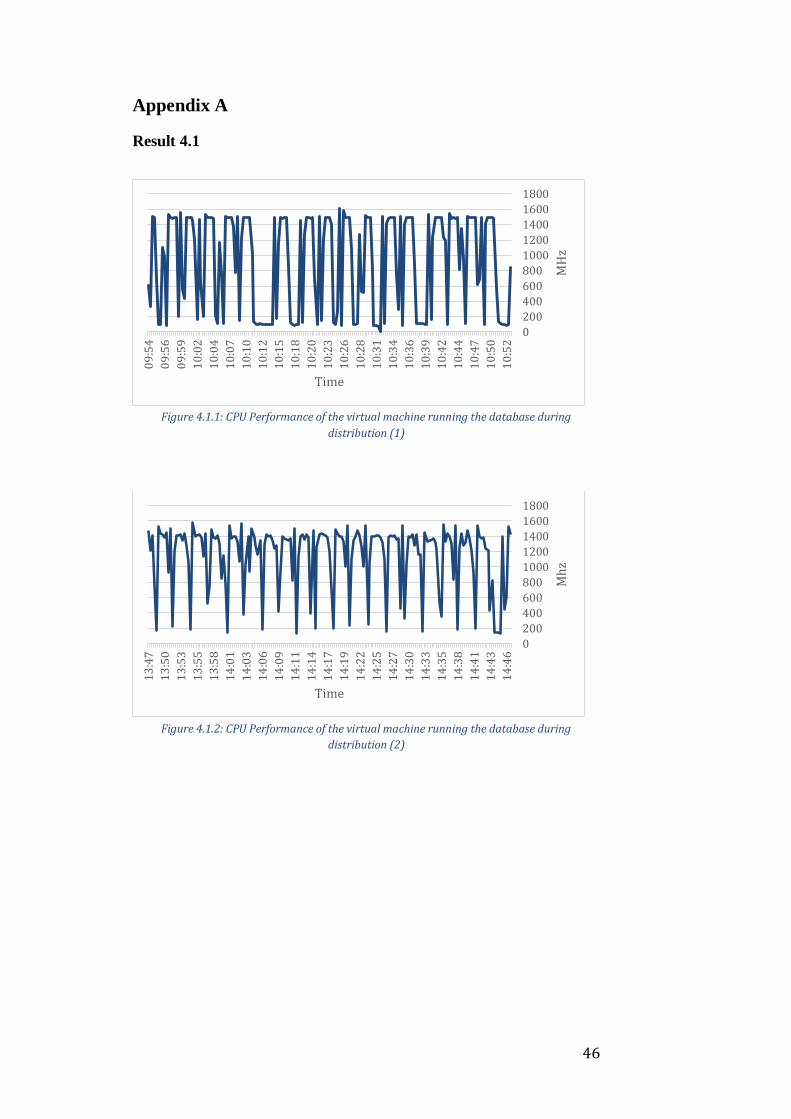
46
Appendix A
Result 4.1
Figure 4.1.1: CPU Performance of the virtual machine running the database during
distribution (1)
Figure 4.1.2: CPU Performance of the virtual machine running the database during
distribution (2)
09
:54
09
:56
09
:59
10
:02
10
:04
10
:07
10
:10
10
:12
10
:15
10
:18
10
:20
10
:23
10
:26
10
:28
10
:31
10
:34
10
:36
10
:39
10
:42
10
:44
10
:47
10
:50
10
:52
0
200
400
600
800
1000
1200
1400
1600
1800
Time
MH
z
13
:47
13
:50
13
:53
13
:55
13
:58
14
:01
14
:03
14
:06
14
:09
14
:11
14
:14
14
:17
14
:19
14
:22
14
:25
14
:27
14
:30
14
:33
14
:35
14
:38
14
:41
14
:43
14
:46
0
200
400
600
800
1000
1200
1400
1600
1800
Time
Mh
z
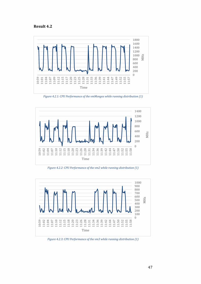
47
Result 4.2
Figure 4.2.1: CPU Performance of the vmMongos while running distribution (1)
Figure 4.2.2: CPU Performance of the vm2 while running distribution (1)
Figure 4.2.3: CPU Performance of the vm3 while running distribution (1)
10
:59
11
:01
11
:04
11
:07
11
:09
11
:12
11
:15
11
:17
11
:20
11
:23
11
:25
11
:28
11
:31
11
:33
11
:36
11
:39
11
:41
11
:44
11
:47
11
:49
11
:52
11
:55
11
:57
0
200
400
600
800
1000
1200
1400
1600
1800
Time
MH
z
10
:59
11
:02
11
:04
11
:07
11
:10
11
:12
11
:15
11
:18
11
:20
11
:23
11
:26
11
:28
11
:31
11
:34
11
:36
11
:39
11
:42
11
:44
11
:47
11
:50
11
:52
11
:55
11
:58
0
200
400
600
800
1000
1200
1400
Time
MH
z
10
:59
11
:02
11
:04
11
:07
11
:10
11
:12
11
:15
11
:18
11
:20
11
:23
11
:26
11
:28
11
:31
11
:34
11
:36
11
:39
11
:42
11
:44
11
:47
11
:50
11
:52
11
:55
11
:58
01002003004005006007008009001000
Time
MH
z
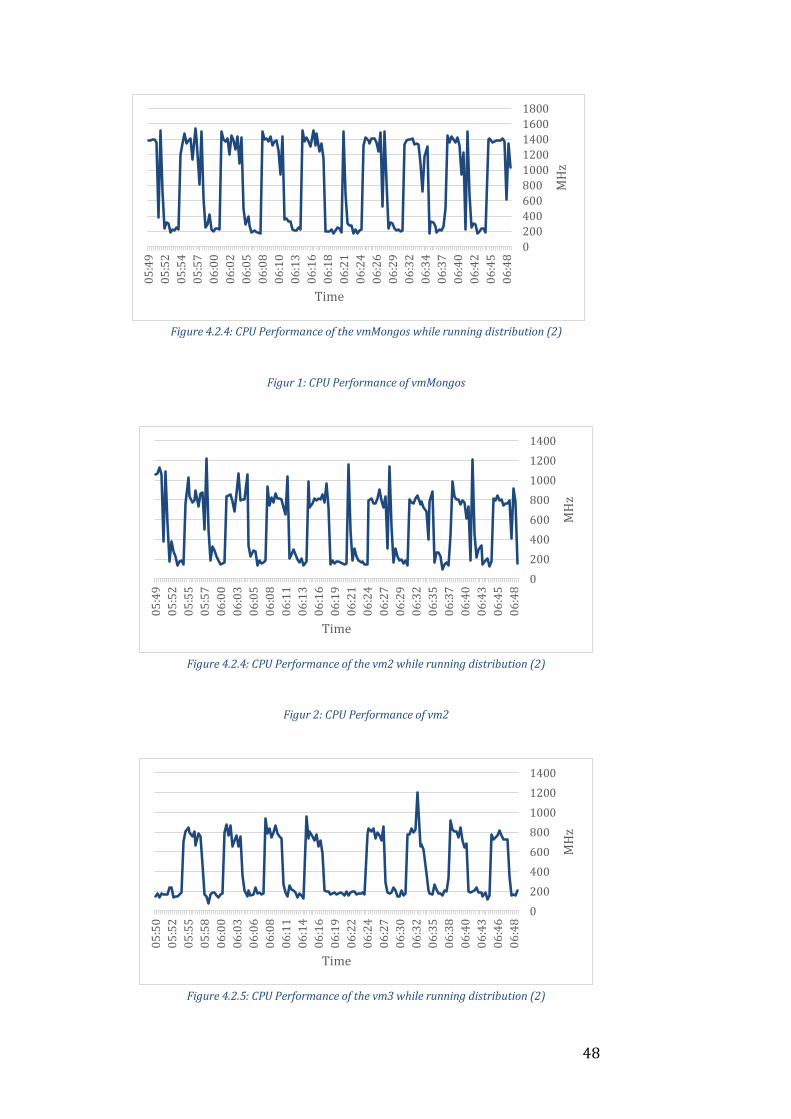
48
Figure 4.2.4: CPU Performance of the vmMongos while running distribution (2)
Figur 1: CPU Performance of vmMongos
Figure 4.2.4: CPU Performance of the vm2 while running distribution (2)
Figur 2: CPU Performance of vm2
Figure 4.2.5: CPU Performance of the vm3 while running distribution (2)
05
:49
05
:52
05
:54
05
:57
06
:00
06
:02
06
:05
06
:08
06
:10
06
:13
06
:16
06
:18
06
:21
06
:24
06
:26
06
:29
06
:32
06
:34
06
:37
06
:40
06
:42
06
:45
06
:48
0
200
400
600
800
1000
1200
1400
1600
1800
Time
MH
z
05
:49
05
:52
05
:55
05
:57
06
:00
06
:03
06
:05
06
:08
06
:11
06
:13
06
:16
06
:19
06
:21
06
:24
06
:27
06
:29
06
:32
06
:35
06
:37
06
:40
06
:43
06
:45
06
:48
0
200
400
600
800
1000
1200
1400
Time
MH
z
05
:50
05
:52
05
:55
05
:58
06
:00
06
:03
06
:06
06
:08
06
:11
06
:14
06
:16
06
:19
06
:22
06
:24
06
:27
06
:30
06
:32
06
:35
06
:38
06
:40
06
:43
06
:46
06
:48
0
200
400
600
800
1000
1200
1400
Time
MH
z
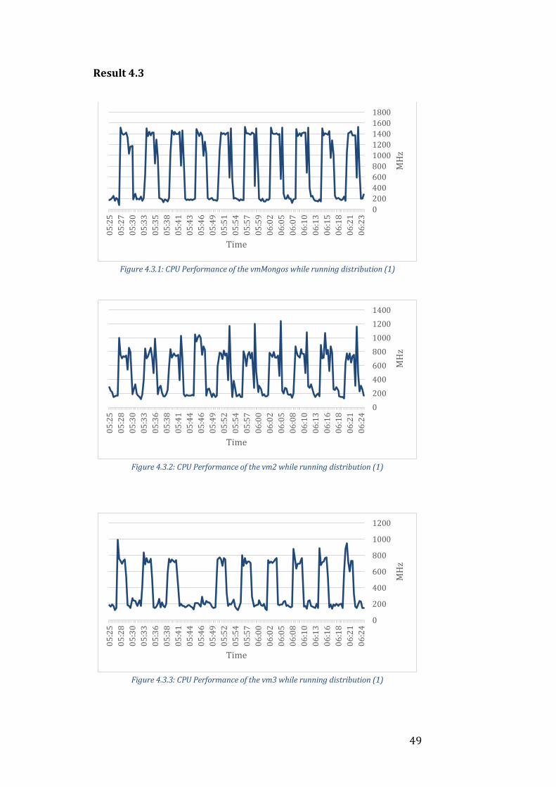
49
Result 4.3
Figure 4.3.1: CPU Performance of the vmMongos while running distribution (1)
Figure 4.3.2: CPU Performance of the vm2 while running distribution (1)
Figure 4.3.3: CPU Performance of the vm3 while running distribution (1)
05
:25
05
:27
05
:30
05
:33
05
:35
05
:38
05
:41
05
:43
05
:46
05
:49
05
:51
05
:54
05
:57
05
:59
06
:02
06
:05
06
:07
06
:10
06
:13
06
:15
06
:18
06
:21
06
:23
0
200
400
600
800
1000
1200
1400
1600
1800
Time
MH
z
05
:25
05
:28
05
:30
05
:33
05
:36
05
:38
05
:41
05
:44
05
:46
05
:49
05
:52
05
:54
05
:57
06
:00
06
:02
06
:05
06
:08
06
:10
06
:13
06
:16
06
:18
06
:21
06
:24
0
200
400
600
800
1000
1200
1400
Time
MH
z
05
:25
05
:28
05
:30
05
:33
05
:36
05
:38
05
:41
05
:44
05
:46
05
:49
05
:52
05
:54
05
:57
06
:00
06
:02
06
:05
06
:08
06
:10
06
:13
06
:16
06
:18
06
:21
06
:24
0
200
400
600
800
1000
1200
Time
MH
z
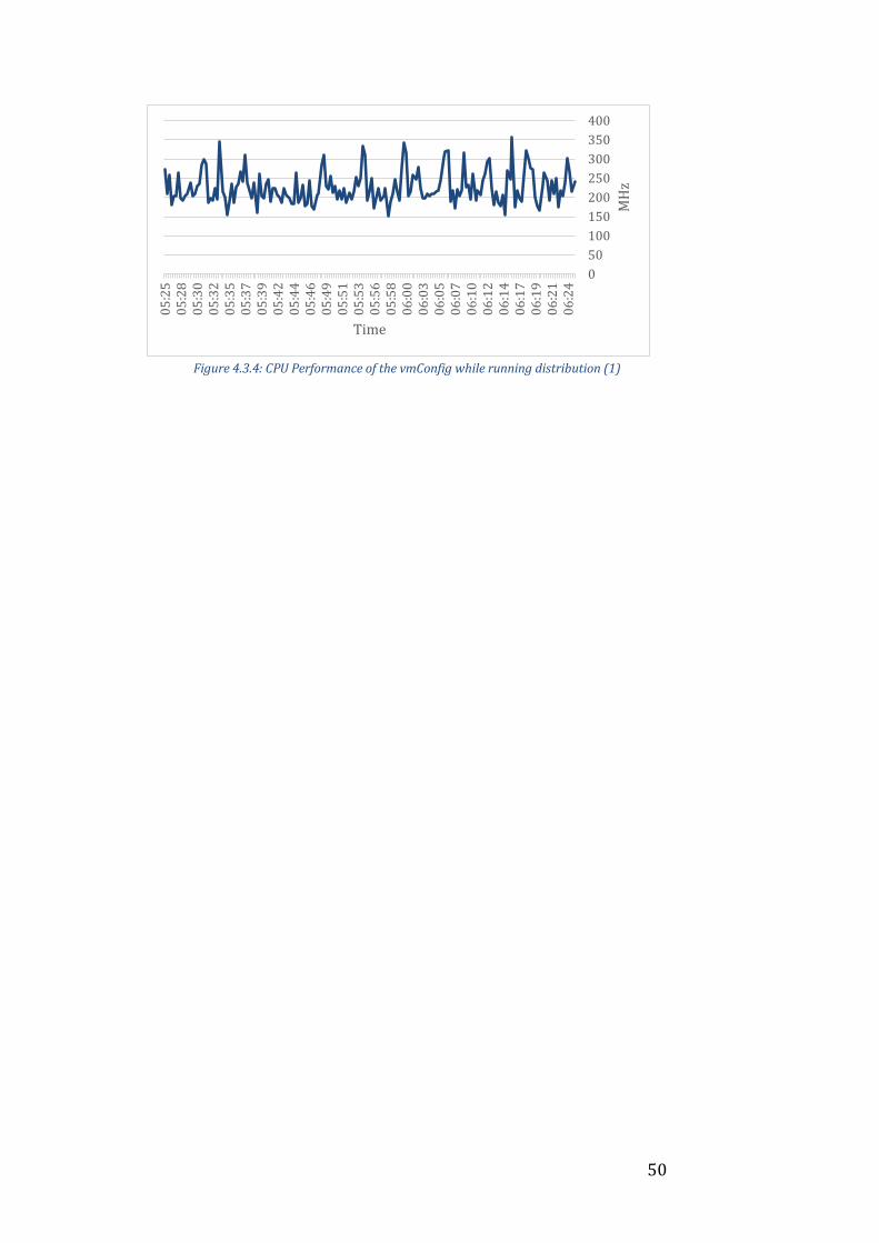
50
Figure 4.3.4: CPU Performance of the vmConfig while running distribution (1)
05
:25
05
:28
05
:30
05
:32
05
:35
05
:37
05
:39
05
:42
05
:44
05
:46
05
:49
05
:51
05
:53
05
:56
05
:58
06
:00
06
:03
06
:05
06
:07
06
:10
06
:12
06
:14
06
:17
06
:19
06
:21
06
:24
0
50
100
150
200
250
300
350
400
Time
MH
z
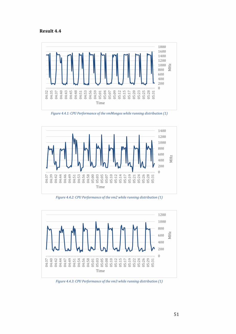
51
Result 4.4
Figure 4.4.1: CPU Performance of the vmMongos while running distribution (1)
Figure 4.4.2: CPU Performance of the vm2 while running distribution (1)
Figure 4.4.3: CPU Performance of the vm3 while running distribution (1)
04
:32
04
:35
04
:37
04
:40
04
:43
04
:45
04
:48
04
:51
04
:53
04
:56
04
:59
05
:01
05
:04
05
:07
05
:09
05
:12
05
:15
05
:17
05
:20
05
:23
05
:25
05
:28
05
:31
0
200
400
600
800
1000
1200
1400
1600
1800
Time
MH
z
04
:37
04
:39
04
:42
04
:44
04
:46
04
:49
04
:51
04
:53
04
:56
04
:58
05
:00
05
:03
05
:05
05
:07
05
:10
05
:12
05
:14
05
:17
05
:19
05
:21
05
:24
05
:26
05
:28
05
:31
0
200
400
600
800
1000
1200
1400
Time
MH
z
04
:37
04
:40
04
:42
04
:44
04
:47
04
:49
04
:51
04
:54
04
:56
04
:58
05
:01
05
:03
05
:05
05
:08
05
:10
05
:12
05
:15
05
:17
05
:19
05
:22
05
:24
05
:26
05
:29
05
:31
0
200
400
600
800
1000
1200
Time
MH
z
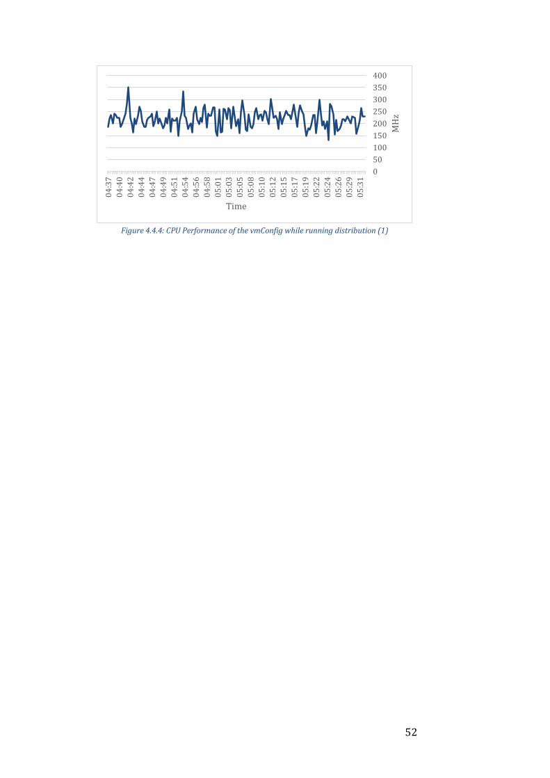
52
Figure 4.4.4: CPU Performance of the vmConfig while running distribution (1)
04
:37
04
:40
04
:42
04
:44
04
:47
04
:49
04
:51
04
:54
04
:56
04
:58
05
:01
05
:03
05
:05
05
:08
05
:10
05
:12
05
:15
05
:17
05
:19
05
:22
05
:24
05
:26
05
:29
05
:31
0
50
100
150
200
250
300
350
400
Time
MH
z
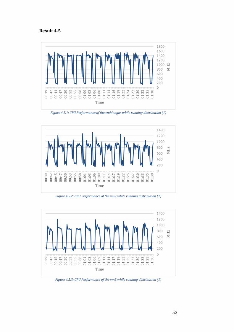
53
Result 4.5
Figure 4.5.1: CPU Performance of the vmMongos while running distribution (1)
Figure 4.5.2: CPU Performance of the vm2 while running distribution (1)
Figure 4.5.3: CPU Performance of the vm3 while running distribution (1)
00
:39
00
:42
00
:44
00
:47
00
:50
00
:52
00
:55
00
:58
01
:00
01
:03
01
:06
01
:08
01
:11
01
:14
01
:16
01
:19
01
:22
01
:24
01
:27
01
:30
01
:32
01
:35
01
:38
0
200
400
600
800
1000
1200
1400
1600
1800
Time
MH
z
00
:39
00
:42
00
:45
00
:47
00
:50
00
:53
00
:55
00
:58
01
:01
01
:03
01
:06
01
:09
01
:11
01
:14
01
:17
01
:19
01
:22
01
:25
01
:27
01
:30
01
:33
01
:35
01
:38
0
200
400
600
800
1000
1200
1400
Time
MH
z
00
:39
00
:42
00
:45
00
:47
00
:50
00
:53
00
:55
00
:58
01
:01
01
:03
01
:06
01
:09
01
:11
01
:14
01
:17
01
:19
01
:22
01
:25
01
:27
01
:30
01
:33
01
:35
01
:38
0
200
400
600
800
1000
1200
1400
Time
MH
z
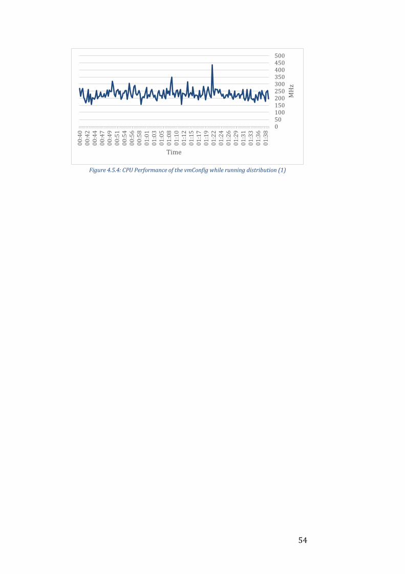
54
Figure 4.5.4: CPU Performance of the vmConfig while running distribution (1)
00
:40
00
:42
00
:44
00
:47
00
:49
00
:51
00
:54
00
:56
00
:58
01
:01
01
:03
01
:05
01
:08
01
:10
01
:12
01
:15
01
:17
01
:19
01
:22
01
:24
01
:26
01
:29
01
:31
01
:33
01
:36
01
:38
050100150200250300350400450500
Time
MH
z

55
Result 4.6
Figure 4.6.1: CPU Performance of the vm1 while running distribution (1)
Figure 4.6.2: CPU Performance of the vm2 while running distribution (1)
Figure 4.6.3: CPU Performance of the vmConfig while running distribution (1)
05
:30
05
:32
05
:35
05
:38
05
:40
05
:43
05
:46
05
:48
05
:51
05
:54
05
:56
05
:59
06
:02
06
:04
06
:07
06
:10
06
:12
06
:15
06
:18
06
:20
06
:23
06
:26
06
:28
0
200
400
600
800
1000
1200
1400
1600
1800
Time
MH
z
05
:30
05
:32
05
:35
05
:38
05
:40
05
:43
05
:46
05
:48
05
:51
05
:54
05
:56
05
:59
06
:02
06
:04
06
:07
06
:10
06
:12
06
:15
06
:18
06
:20
06
:23
06
:26
06
:28
0
200
400
600
800
1000
1200
1400
1600
1800
Time
MH
z
05
:30
05
:32
05
:35
05
:37
05
:39
05
:42
05
:44
05
:46
05
:49
05
:51
05
:53
05
:56
05
:58
06
:00
06
:03
06
:05
06
:07
06
:10
06
:12
06
:14
06
:17
06
:19
06
:21
06
:24
06
:26
06
:28
0
50
100
150
200
250
300
350
400
Time
MH
z
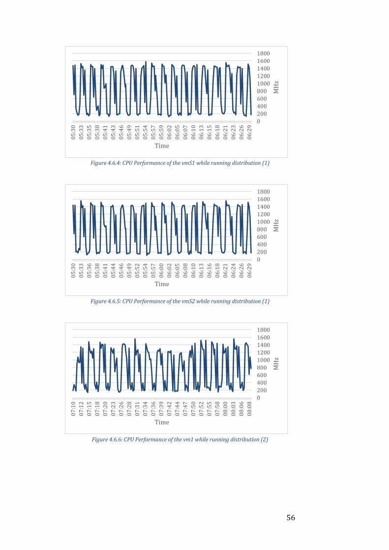
56
Figure 4.6.4: CPU Performance of the vmS1 while running distribution (1)
Figure 4.6.5: CPU Performance of the vmS2 while running distribution (1)
Figure 4.6.6: CPU Performance of the vm1 while running distribution (2)
05
:30
05
:33
05
:35
05
:38
05
:41
05
:43
05
:46
05
:49
05
:51
05
:54
05
:57
05
:59
06
:02
06
:05
06
:07
06
:10
06
:13
06
:15
06
:18
06
:21
06
:23
06
:26
06
:29
0
200
400
600
800
1000
1200
1400
1600
1800
Time
MH
z
05
:30
05
:33
05
:36
05
:38
05
:41
05
:44
05
:46
05
:49
05
:52
05
:54
05
:57
06
:00
06
:02
06
:05
06
:08
06
:10
06
:13
06
:16
06
:18
06
:21
06
:24
06
:26
06
:29
0
200
400
600
800
1000
1200
1400
1600
1800
Time
MH
z
07
:10
07
:12
07
:15
07
:18
07
:20
07
:23
07
:26
07
:28
07
:31
07
:34
07
:36
07
:39
07
:42
07
:44
07
:47
07
:50
07
:52
07
:55
07
:58
08
:00
08
:03
08
:06
08
:08
0
200
400
600
800
1000
1200
1400
1600
1800
Time
MH
z
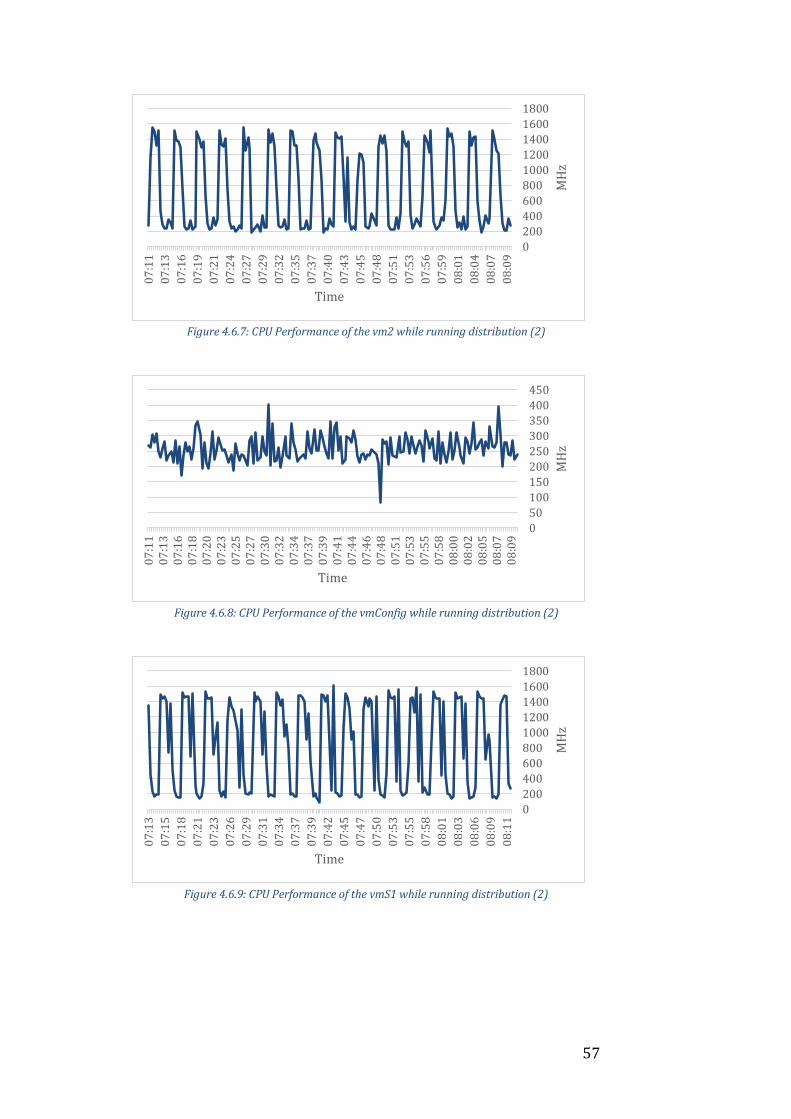
57
Figure 4.6.7: CPU Performance of the vm2 while running distribution (2)
Figure 4.6.8: CPU Performance of the vmConfig while running distribution (2)
Figure 4.6.9: CPU Performance of the vmS1 while running distribution (2)
07
:11
07
:13
07
:16
07
:19
07
:21
07
:24
07
:27
07
:29
07
:32
07
:35
07
:37
07
:40
07
:43
07
:45
07
:48
07
:51
07
:53
07
:56
07
:59
08
:01
08
:04
08
:07
08
:09
0
200
400
600
800
1000
1200
1400
1600
1800
Time
MH
z
07
:11
07
:13
07
:16
07
:18
07
:20
07
:23
07
:25
07
:27
07
:30
07
:32
07
:34
07
:37
07
:39
07
:41
07
:44
07
:46
07
:48
07
:51
07
:53
07
:55
07
:58
08
:00
08
:02
08
:05
08
:07
08
:09
0
50
100
150
200
250
300
350
400
450
Time
MH
z
07
:13
07
:15
07
:18
07
:21
07
:23
07
:26
07
:29
07
:31
07
:34
07
:37
07
:39
07
:42
07
:45
07
:47
07
:50
07
:53
07
:55
07
:58
08
:01
08
:03
08
:06
08
:09
08
:11
0
200
400
600
800
1000
1200
1400
1600
1800
Time
MH
z
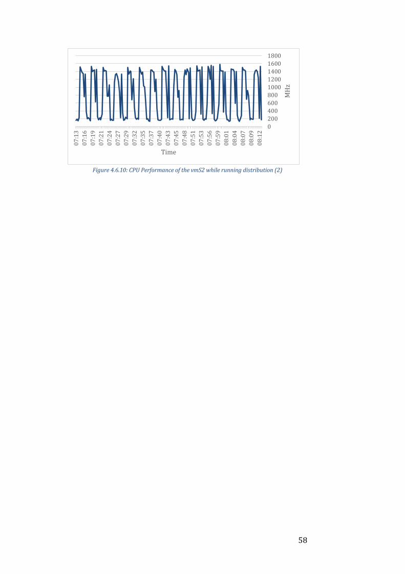
58
Figure 4.6.10: CPU Performance of the vmS2 while running distribution (2)
07
:13
07
:16
07
:19
07
:21
07
:24
07
:27
07
:29
07
:32
07
:35
07
:37
07
:40
07
:43
07
:45
07
:48
07
:51
07
:53
07
:56
07
:59
08
:01
08
:04
08
:07
08
:09
08
:12
0
200
400
600
800
1000
1200
1400
1600
1800
Time
MH
z
Top Related