


Languages
Pages
Legal


1
Developing a Long Term Strategy for a Warehouse Network by
Patrick Johnson
B.S. Industrial and Systems Engineering, Auburn University, 2008
Submitted to the Sloan School of Management and the Institute for Data, Systems, and Society in
partial fulfillment of the requirements for the degrees of
Master of Science in Engineering Systems
And Master of Business Administration
In conjunction with the Leaders for Global Operations Program at the Massachusetts Institute of Technology
June 2017
© 2017 Patrick Johnson. All rights reserved.
The author hereby grants to MIT permission to reproduce and to distribute publicly paper and electronic copies of this thesis document in whole or in part in any medium now known or hereafter created
Signature of Author ____________________________________________________________________
MIT Sloan School of Management, Institute for Data, Systems, and Society May 12, 2017
Certified by __________________________________________________________________________
David Simchi-Levi, Thesis Supervisor Professor of Engineering Systems, Institute for Data, Systems, and Society
Certified by __________________________________________________________________________ Donald Rosenfield, Thesis Supervisor
Senior Lecturer, MIT Sloan School of Management
Accepted by __________________________________________________________________________ John N. Tsitsiklis, Clarence J. Lebel Professor of Electrical Engineering
IDSS Graduate Officer Accepted by __________________________________________________________________________
Maura Herson, Director, MBA Program MIT Sloan School of Management

2
This page intentionally left blank.

3
Abstract
This thesis addresses the question of how to create a pro-active, long term, network centric warehouse strategy. This thesis will present an inventory model built to understand the capacity needs of Amgen’s warehouses over the time period of 2017-2023 to support this mission, along with recommendations based on scenario analysis from this model to analyze and quantify the impacts of multiple scenarios in support of an efficient, effective, nimble supply chain.
With worldwide operations supporting a global customer base, Amgen’s operational philosophy is to ensure serving “every patient, every time”. Amgen’s warehouses play a vital role with this mission, storing raw materials to ensure production with safety stock and various levels of Work in Progress (WIP) based not only on operational safety stock, but also strategic safety stock to ensure demand is always met, even with unforeseen risks.
In order to understand the impacts of growth on warehouse utilization, a relational database inventory model was created and linked to the long range forecast of supply and demand. This inventory model linked the Bill of Materials (BOMs) to the product forecast in order to to understand the quantity of raw materials required to meet the supply. The database also calculates the WIP and finished product levels of Amgen’s products. This model considers inefficiencies in the warehouses, as warehouse pallet spaces do not always store the maximum capacity of the material.
This inventory model calculated the capacity required for each warehouse over the forecasted ranges of FY 2016 to FY 2023. The findings of this model were used to create Amgen’s long term warehouse strategy. The model demonstrated a +- 10% accuracy to 2017 planning.
We developed a strategy that mimics Amgen’s operational strategy. Amgen’s operational strategy is to reduce fixed costs, and focus on flexibility with variable based costs. Based on this, we found the best strategy was to work with 3rd party logistics providers (3PLs) to mitigate the capacity gaps in a variable based manner. This option is preferred over investing in expanding capacity at warehouses already in use for all three scenarios of optimistic, baseline, and pessimistic demand profiles.
The biggest lever to gain warehouse capacity is to improve inventory policies and the flow of communication. Inventory policies whose aim is to reduce inventory can be viewed as a sensitive topic at a company like Amgen. But, if done in a scientific manner, and moving from a Months on Hand (MOH) approach to a scientifically calculated inventory, then moving to a multi-echelon inventory optimization, inventory and risk can be reduced. The following are ways that can be used to reduce inventory and risks.
Track forecast error to understand variation of demand
Lead time reduction of raw materials and work in progress
Risk Pool Drug Product (DP) “nude” vials and decrease lead time from DP to customer
Re-order point frequency increases
Reduction of demand variability through: o Better communication of demand forecasts between marketing, global supply chain
and site supply chain teams. o Reducing variability of manufacturing planning
Seek commonality of raw materials to lower safety stock levels
Multi-Echelon Inventory Optimization

4
By accomplishing these activities, Amgen has a scope to reduce 3PL storage requirements by 20k pallet-year spaces over the same time period. This will lower the expense of 3PL costs, and overall risks, over the same time period by $11 M. Considerable work will have to be accomplished, but the benefits will outweigh the costs.
Thesis Supervisor: Donald Rosenfield Title: Senior Lecturer, MIT Sloan School of Management Thesis Supervisor: David Simchi-Levi Title: Professor of Engineering Systems, Institute for Data, Systems, and Society
5
Acknowledgements No man is an Island - John Donne
I’d like to thank the Leaders for Global Operations Program for its support of this work. Amgen
has been a gracious company throughout this project with support, encouragement, and proper
feedback. More specifically, I’d like to thank Delia Sander for her never-ending support with all of the
knowledge and experience she brought to this project. Tarun Bhatia was instrumental in keeping the
high level impact of this project at the forefront, ensuring we focus on the big picture. As the saying
goes, “I apologize for the long letter, as I didn’t have the time to write a shorter one.” Tarun has ensured
we communicated the main message of this project to the network effectively. Venkat Subramanian
was a tremendous help in ensuring focus and support on this project, navigating a tricky software
procurement process with ease. Cathryn Shaw-Reid was gracious with her time sharing the bigger
impact of how this project fits in with Amgen, and how I can help support that mission.
David-Simchi Levi, Sean Willems, and Donald Rosenfield, three brilliant professors, were always
just an email or phone call away to offer light when I seemed lost in the dark. Two LGO alumni, Steve
Fuller and Seth White, were so important in helping to determine which data to use to support the
model displayed in this paper and where to find it. They also ensured I understood the limitations of
this data.
Lastly, I’d like to thank Megan Johnson for her constant encouragement and support, being
patient as I ruined another hike with her by thinking out loud about the intricacies of the model
developed in this paper. She has always been ready for another adventure, and this certainly was one
as we moved across the country to pursue this challenging opportunity.

6
Table of Contents Abstract ......................................................................................................................................................... 3
Acknowledgements ....................................................................................................................................... 5
Table of Contents .......................................................................................................................................... 6
List of Tables ................................................................................................................................................. 8
List of Figures ................................................................................................................................................ 9
List of Equations .......................................................................................................................................... 10
1 Introduction ........................................................................................................................................ 11
1.1 Project Situation ...................................................................................................................... 11
1.2 Project Motivation .................................................................................................................. 12
1.3 Problem Statement ................................................................................................................. 12
1.4 Thesis Goals ............................................................................................................................. 12
1.5 Thesis Scope ............................................................................................................................ 13
1.6 Thesis Overview ...................................................................................................................... 13
2 Operations at Amgen .......................................................................................................................... 14
2.1 Company History ..................................................................................................................... 14
2.2 Company Therapeutics ........................................................................................................... 15
2.3 Operations Overview .............................................................................................................. 18
2.4 Manufacturing Overview ........................................................................................................ 21
2.5 Warehouse Operations Overview ........................................................................................... 24
2.6 Supply Chain Operations Overview ........................................................................................ 27
2.7 Long Range Plan Overview ...................................................................................................... 31
3 Literature Review ................................................................................................................................ 33
3.1 Amgen’s Operations in Literature ........................................................................................... 33
3.2 Broader Themes in Literature relevant to this case................................................................ 34
4 Methodology ....................................................................................................................................... 42
4.1 Current State Analysis ............................................................................................................. 42
4.2 Baseline Warehouse Capacity Model Creation ....................................................................... 43
4.3 Warehouse Capacity Scenario Creation .................................................................................. 48
5 Results and Recommendations ........................................................................................................... 52
5.1 Model Results.......................................................................................................................... 52
5.2 Warehouse Strategy Creation ................................................................................................. 54

7
5.3 Supply Chain Communication ................................................................................................. 56
5.4 Risk Mitigation Plan ................................................................................................................ 57
6 Future Work ........................................................................................................................................ 57
7 Conclusion ........................................................................................................................................... 59
8 References .......................................................................................................................................... 62
Appendix 1: Warehouse Capacity Model Details........................................................................................ 64
Baseline Model............................................................................................................................................ 65
Inputs: ..................................................................................................................................................... 65
Queries: ................................................................................................................................................... 65
Outputs: .................................................................................................................................................. 67
Risk Assessment .......................................................................................................................................... 67
Inputs: ..................................................................................................................................................... 68
Queries: ................................................................................................................................................... 68
Outputs: .................................................................................................................................................. 68
Optimistic and Pessimistic Scenarios .......................................................................................................... 68
Inputs: ..................................................................................................................................................... 68
Queries & Outputs: ................................................................................................................................. 68

8
List of Tables Table 1: Comparison of Amgen’s Financial Metrics vs. Other Bio-tech Companies ................................... 21
Table 2: Comparison of Safety Stock levels through lead time reduction .................................................. 40
Table 3: Column Name and Column Descriptions of model output ........................................................... 52
Table 4: Capacity Utilization of baseline model for each warehouse by temperature type ...................... 53
Table 5: Model Predictions of over-utilization associated expense based on demand scenarios ............. 53
Table 6: Model predictions of over-utilization associated expense of warehouse network ...................... 54
Table 7: Site NPV 3PL expense based on demand scenarios ...................................................................... 58

9
List of Figures Figure 1: Breakdown of Amgen’s Therapeutics by Revenue for FY 2015 (Amgen, 2016) .......................... 16
Figure 2: Conditional Probability of Success for Drug Trials 2000-2013 ..................................................... 17
Figure 3: A Simplified Example of Amgen’s Supply Chain Operations ........................................................ 20
Figure 4: Manufacturing Process Flow of Bio-Technology and the Corresponding Inventory ................... 22
Figure 5: Hypothetical Material Consumption Forecast ............................................................................. 23
Figure 6: cGMP Raw Material Checklist ...................................................................................................... 25
Figure 7: Global View of Amgen’s Commercial Manufacturing, Warehousing, and Distribution Centers . 26
Figure 8: Distribution of Last Stock Placement (in Days) for Amgen’s Warehouses .................................. 27
Figure 9: Amgen’s Work in Progress Inventory Levels ................................................................................ 28
Figure 10: Distribution of frequency of lead time (in days) of raw materials ............................................. 31
Figure 12: The Three Frontiers of Inventory Optimization (Willems, 2015) ............................................... 36
Figure 13: Example of a bull whip effect from point of sale to manufacturer ........................................... 37
Figure 11: Biopharma demand and forecast variation analysis (Rosenfield, 2014) ................................... 39
Figure 14: Demand Profiles for Optimistic and Pessimistic Pipeline and Commercial Therapeutics ......... 49

10
List of Equations Equation 1: Average Cycle Stock Calculation .............................................................................................. 28
Equation 2: Order Size Calculation ............................................................................................................. 28
Equation 3: Calculation of Safety Stock ...................................................................................................... 29
Equation 4: Calculation of Projected Balance ............................................................................................. 32
Equation 5: Inventory equations from demand forecast and lead time .................................................... 39
Equation 6: Safety Stock Reduction through Lead Time Reduction ........................................................... 40
Equation 7: Months on Hand Calculation ................................................................................................... 45
Equation 8: Calculations of Pallet spaces required for Pipeline Therapeutics with no known BOM’s ....... 45
Equation 9: Pallets of Projected Balance .................................................................................................... 45
Equation 10: Calculation of Raw Material .................................................................................................. 46
Equation 11: Calculation of WIP Inventory ................................................................................................. 46
Equation 12: Pallet Efficiency ...................................................................................................................... 47
Equation 13: Warehouse Capacity Utilization ............................................................................................ 47
Equation 14: Pallets over Capacity summation .......................................................................................... 47
Equation 15: 3PL Cost for adding additional capacity ................................................................................ 47
Equation 16: Net Present Value Calculation ............................................................................................... 48
Equation 17: Equation for Commercial and Therapeutics Multiplier ......................................................... 49
Equation 18: Warehouse Capacity Adjustment for Optimistic and Pessimistic Scenarios ......................... 50
Equation 19: Warehouse Capacity Utilization at Standard Utilization ....................................................... 51
Equation 20: Revised Pallets of inventory for Inventory Policy changes .................................................... 52

11
1 Introduction
1.1 Project Situation
The sea gets deeper as you go further into it – Phoenician Proverb
This thesis is a result of a research project with Amgen in Thousand Oaks, California as a fellow
in the Massachusetts Institute of Technology Leaders for Global Operations program. The research
project is a research-based component of the two year duel-degree program for a Masters of Business
Administration and a Masters of Systems Engineering.
Amgen is a biopharmaceutical company whose mission is to “Serve Patients”. Their operating
philosophy is to serve “every patient, every time”. They take this philosophy seriously, being only one of
two bio-tech companies who have never stocked out of their life saving therapeutics for patients. This
philosophy is shown in the balance sheet, with over $2.4B in inventory on $20.9B of revenue for Fiscal
Year (FY) 2015 (Amgen, 2016). Amgen has a network of global warehouses that store inventory in
support of this mission. These warehouses not only store raw materials with the corresponding
operational safety stock and work in progress (WIP), but also strategic safety stock. This strategic safety
stock is WIP at different stages of manufacturing stored to ensure patients will be served if any
manufacturing capacity is lost to unplanned risks.
Amgen has a highly variable ten year forecast of their existing therapeutics, called the Long
Range Plan (LRP) due to the following:
A strong pipeline of developing drugs that may or may not be approved by the FDA.
A propensity for acquisitions of other late stage drug therapeutics from other
companies.
Offering its therapeutics to more global markets, serving more countries.
Amgen currently has an excel-based model for individual warehouses that will show capacity
utilization monthly over a rolling two years, but no pro-active, network-centric model or warehouse

12
strategy exists in support of the Long Range Plan. Due to this, warehouse managers and global supply
chain managers make sub-optimal decisions when it comes to the storing of therapeutics, where some
warehouses buy extra capacity in their respective local markets due to being over utilized, while at the
same time other warehouses are underutilized.
1.2 Project Motivation
The motivation for this project is to ensure Amgen will be able to serve “every patient, every
time” with a superior warehouse strategy. By creating a robust model that runs scenarios to simulate
variations in demand profiles and changes in operating variables, an analysis can be created to identify
over-utilization of capacity in the warehouse network and identify the best solutions to mitigate costly
reactive decisions.
1.3 Problem Statement
Currently, there is no pro-active, long term, network centric strategy for Amgen’s warehouses.
Warehouse managers manage their respective warehouses and supply chain managers flow their
respective therapeutics through warehouses without regard to the entire network. This leads to some
warehouses being over-utilized; which in turn leads to storage at 3rd Party Logistics providers (3PL’s);
while other warehouses suffer from underutilization. Amgen forecast for future demand is highly
variable, leading to reactive decisions in order to ensure warehouse capacity is available to store both
raw materials and therapeutics.
1.4 Thesis Goals
The goal of this thesis is to create a warehouse strategy that will allow Amgen to nimbly,
efficiently, and efficiently serve patients. To support this strategy, a model of the warehouse inventory
requirements linked to Amgen’s Long Range Plan will need to be created. This model will identify the
capacity gaps based on a variety of scenarios and the effects of capacity gap mitigations on the network.
13
Recommendations will be analyzed and given to ensure an efficient, effective, and nimble strategy is
thoroughly communicated.
1.5 Thesis Scope
The scope of this analysis will be Amgen’s internal commercial production and warehouse
system. More specifically, the capacity of Controlled Room Temperature (CRT)/ Ambient and 2-8°C
warehouse storage. Due to 3rd party manufacturing and distributors storing raw materials, WIP, and
finished therapeutics at their own sites, they are out of scope. Due to the nature of clinical productions
unknown demand and frequent schedule changes, clinical production and storage are out of scope. Also
out of scope are the warehouse freezers and warehouse hazmat storage, as this storage is relatively
small, and additional capacity can be added relatively quickly. The impacts of financial costs of moving
inventory frictionless from one global location to another are also out of scope. Due to this significant
factor, no new shipping lanes (nodes) were created or analyzed, as the impacts of the tax situation could
possibly outweigh the benefits of lowering over-utilization.
1.6 Thesis Overview
This thesis is categorized by chapters in a way to understand the project first from a high level
view of the industry and company, then dive deeper into the finer details of the warehouse strategy
creation through model developed. The contents of each chapter can be briefly described as follows:
Chapter 2 will begin with an overview of the Amgen’s history, line of therapeutics, and future
therapeutics. This chapter will also provide an overview of Amgen’s operations, and more specifically,
warehouse and supply chain operations and the Long Range Plan.
Chapter 3 will provide a review of literature to showcase best practices for strategy creation and
warehouse operations, along with a review of research on warehouse networks. It will also include a
review of standard inventory policies.

14
Chapter 4 will detail the approach to solving the problem statement. This chapter contains the
detailed steps of building the warehouse capacity model to support the strategy development, along
with the equations. This chapter will also detail the scenarios built to understand the implications of
changes in key assumptions in the model, along with scenarios to mitigate overutilization of the
capacity.
Chapter 5 will detail the results and implications of the baseline model, along with the different
scenarios. It will also detail recommendations for best practices and how to alleviate overutilization of
the warehouse capacity. This analysis will be used to craft the strategy, which will be detailed.
Chapter 6 will detail future projects that could be taken on to ensure warehouse capacity is
available in the foreseeable future, along with a path forward for inventory optimization to ensure an
efficient, effective, and nimble supply chain.
2 Operations at Amgen
2.1 Company History
Amgen Inc. (Applied Molecular Genetics) is an American multinational biopharmaceutical
company headquartered in Thousand Oaks, California. William Bowes, a frustrated manager at Cetus
Corporation (Author Unknown, 2016), left Cetus and recruited Winston Salser, a UCLA scientist, to begin
Amgen in 1980. Bowes was able to recruit a powerful scientific advisory board and gain initial seed
capital of $200K from venture capitalists. Bowes’ next step was to recruit George Rathmann from
Abbott Laboratories to be the CEO of Amgen. Rathman was able to gain secured private equity funding
from Abbot and Tosco Corporation, which gave confidence to venture capitalist, who in turn invested
$19.4M in the new company. In 1983, Amgen tendered an IPO raising $42.3M.

15
With the financing now in hand, Amgen went to work on genetic engineering. Amgen was able
to isolate and clone the erythropoietin gene, which stimulated red blood cell production. Since they had
enough financing, they were able to forgo licensing the resulting drug (Epogen), and after a lengthy FDA
approval process, gained the right to begin selling Epogen. In 1985, Amgen created a joint venture with
Kirin Brewery to gain access to manufacturing technology in exchange for international marketing rights.
With this manufacturing technology in hand, Epogen became the first biopharmaceutical to gross over
$1B in annual revenue. Amgen has since grown to 20,000 employees with revenues of $21B for FY 2015
(Amgen, 2016), and a market cap of $128B.
2.2 Company Therapeutics
Amgen currently offers 15 innovative therapeutics with a wide variety of applications and
modalities. Figure 1 describes the largest Amgen therapeutics by revenue and the corresponding
revenue growth of those therapeutics. These therapeutics encompass every stage of the therapeutics
life-cycle; from Epogen, which was approved for marketing in 1989 to Kyprolis, which was approved for
treating patients with refractory multiple myeloma in 2016. These therapeutics are encountering
growing competition as some therapeutics are coming off patent which brings on the creation of bio-
similars. A bio-similar is a biological therapeutic that is highly similar to an FDA-approved biological
therapeutics and has no clinically meaningful differences in terms of safety and effectiveness from the
reference therapeutics (Amgen Pipeline, 2016).

16
Figure 1: Breakdown of Amgen’s Therapeutics by Revenue for FY 2015 (Amgen, 2016)
Amgen’s main therapeutics, corresponding markets, and uses are the following:
Enbrel – Marketed primarily in the United States, it is used primarily for the treatment of adult
patients with the following conditions
o Moderately to severely active rheumatoid arthritis,
o Chronic moderate – to – severe plaque psoriasis patients
o Active psoriatic arthritis
Neulasta – Marketed primarily in the United States and Europe, it is used primarily to help
reduce the probability of infection due to low white blood cell count in people with non-myeloid
cancer who receive chemotherapy.
Aranesp – Marketed primarily in the United States and Europe, it is used primarily for the
treatment of anemia.
Epogen – Marketed primarily in the United States, it is used primarily to treat a lower-than-
normal number of red blood cells in patients on dialysis.
17
Sensipar/Mimpara – Sensipar is primarily marketed in the United States and Mimpara is
primarily marketed in Europe. It is used primarily for the treatment of Secondary
hyperparathyroidism in adult patients with Chronic Kidney Disease on dialysis.
Xgeva - Marketed primarily in the United States and Europe, Xgeva is used for prevention of
bone failure in patients with bone metastases from solid tumors and
Prolia- Marketed primarily in the United States and Europe, Prolia is used for treatment of
postmenopausal women with osteoporosis.
Neupogen – Marketed primarily in the United States, Canada, and Europe, it is used primarily to
help reduce infection due to a low white blood cell count in people with non-myeloid cancer
who receive chemotherapy.
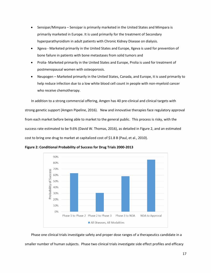
In addition to a strong commercial offering, Amgen has 40 pre-clinical and clinical targets with
strong genetic support (Amgen Pipeline, 2016). New and innovative therapies face regulatory approval
from each market before being able to market to the general public. This process is risky, with the
success rate estimated to be 9.6% (David W. Thomas, 2016), as detailed in Figure 2, and an estimated
cost to bring one drug to market at capitalized cost of $1.8 B (Paul, et al., 2010).
Figure 2: Conditional Probability of Success for Drug Trials 2000-2013
Phase one clinical trials investigate safety and proper dose ranges of a therapeutics candidate in a
smaller number of human subjects. Phase two clinical trials investigate side effect profiles and efficacy

18
of a therapeutics candidate in a large number of patients who have the disease or condition under
study. Phase three clinical trials investigate the safety and efficacy of a therapeutics candidate in a large
number of patients who have the disease or condition under study. As of November 2016, Amgen
presently has fifteen therapeutics candidates in phase one trials, seven therapeutics candidates in Phase
two trails, twelve therapeutics candidates in Phase three trails, and six therapeutics candidates being
developed as Bio-similars. Based on the conditional probabilities for success from Figure 2 Amgen has
an expected value of 8.4 novel therapeutics candidates emerging from trials to approval.
A bio-similar, or follow-on biologic, is a biologic medicine designed to have active properties similar
to one that has been previously been licensed by another company. Bio-similars follow a different
regulatory review pathway than innovative therapeutics and indications. These products do not
command the gross margins that patented products command, but do not face the high development
costs, and risks that that entails, either.
2.3 Operations Overview
Amgen’s operational philosophy is to serve “every patient, every time”. They take great pride in
focusing on the patient, with posters of patients around the office, and most staff meetings starting with
patients talking about how Amgen’s therapeutics have positively impacted their lives. These words are
not taken lightly, and this is shown in their balance sheet and operational strategy. Amgen uses
inventory for the following reasons:
Reduce risk of variation in demand
Reduce risk of variation in supply
Reduce risk of supplier shutdown’s for single-sourced suppliers
Reduce risk of long, variable lead times
Reduce risk of natural/geo-political manufacturing shutdowns
19
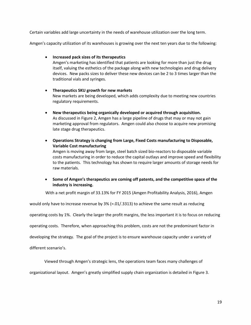
Certain variables add large uncertainty in the needs of warehouse utilization over the long term.
Amgen’s capacity utilization of its warehouses is growing over the next ten years due to the following:
Increased pack sizes of its therapeutics Amgen’s marketing has identified that patients are looking for more than just the drug itself, valuing the esthetics of the package along with new technologies and drug delivery devices. New packs sizes to deliver these new devices can be 2 to 3 times larger than the traditional vials and syringes.
Therapeutics SKU growth for new markets New markets are being developed, which adds complexity due to meeting new countries regulatory requirements.
New therapeutics being organically developed or acquired through acquisition. As discussed in Figure 2, Amgen has a large pipeline of drugs that may or may not gain marketing approval from regulators. Amgen could also choose to acquire new promising late stage drug therapeutics.
Operations Strategy is changing from Large, Fixed Costs manufacturing to Disposable, Variable Cost manufacturing Amgen is moving away from large, steel batch sized bio-reactors to disposable variable costs manufacturing in order to reduce the capital outlays and improve speed and flexibility to the patients. This technology has shown to require larger amounts of storage needs for raw materials.
Some of Amgen’s therapeutics are coming off patents, and the competitive space of the industry is increasing.
With a net profit margin of 33.13% for FY 2015 (Amgen Profitability Analysis, 2016), Amgen
would only have to increase revenue by 3% (=.01/.3313) to achieve the same result as reducing
operating costs by 1%. Clearly the larger the profit margins, the less important it is to focus on reducing
operating costs. Therefore, when approaching this problem, costs are not the predominant factor in
developing the strategy. The goal of the project is to ensure warehouse capacity under a variety of
different scenario’s.
Viewed through Amgen’s strategic lens, the operations team faces many challenges of
organizational layout. Amgen’s greatly simplified supply chain organization is detailed in Figure 3.
20
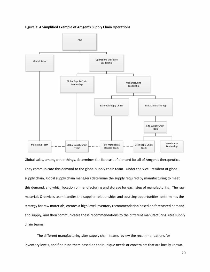
Figure 3: A Simplified Example of Amgen’s Supply Chain Operations
External Supply Chain
Site Supply ChainTeam
Sites Manufacturing
Site Supply Chain Team
Global Sales
Warehouse Leadership
Manufacturing Leadership
Global Supply ChainLeadership
Raw Materials & Devices Team
Global Supply Chain Team
Operations Executive Leadership
Marketing Team
CEO
Global sales, among other things, determines the forecast of demand for all of Amgen’s therapeutics.
They communicate this demand to the global supply chain team. Under the Vice President of global
supply chain, global supply chain managers determine the supply required by manufacturing to meet
this demand, and which location of manufacturing and storage for each step of manufacturing. The raw
materials & devices team handles the supplier relationships and sourcing opportunities, determines the
strategy for raw materials, creates a high level inventory recommendation based on forecasted demand
and supply, and then communicates these recommendations to the different manufacturing sites supply
chain teams.
The different manufacturing sites supply chain teams review the recommendations for
inventory levels, and fine-tune them based on their unique needs or constraints that are locally known.

21
They then place the orders into the ordering system to trigger the orders to the suppliers. The
warehouse leader works with the site’s supply chain teams to understand the short term forecast in
order to understand the warehouse capacity required to accept raw materials, work in progress, and
finished therapeutics when it is shipped to them.
Amgen’s inventory turnover ratio is 1.74, leading to an average days of inventory at 210 days
(Amgen, 2016). Based on a study performed in 2013 (REL , 2013), The U.S. Biotech industry has the 2nd
highest Days of Working Capital (85 days) of all industries, right behind aerospace. Comparing inventory
ratio’s to other bio-tech companies, Amgen has a lower inventory turnover, lower working capital
turnover, higher days of inventory, and a longer cash conversion cycle, as shown in Table 1. While this
table shows that Amgen has room for improvement among its peers, it should be noted that Amgen is
only 1 of 2 bio-tech companies to have never stocked out of thereputics to patients.
Table 1: Comparison of Amgen’s Financial Metrics vs. Other Bio-tech Companies
2.4 Manufacturing Overview
Amgen’s manufacturing operations are a tremendous competitive advantage. The high level
manufacturing flow for bio-tech begins with selecting a cell from a cell bank with the given medicinal
properties. The cell is transferred to a beaker and fed various ingredients as the cell enters geometric
growth. This growth is the bottleneck of the process, where cells double every 24 hours. The cells are
systematically transferred to larger and larger vessels ensuring proper oxygen levels, pH, and
temperatures for optimal growth. When the cell produces the protein, and the cells are at the
necessary volume, the cell is broken up and the protein is harvested. Stabilizing ingredients are
AMGEN Merck Gilead
Inventory Turnover 1.74 3.18 2.05
Working Capital Turnover 0.7 3.74 2.16
Days of Inventory 210 115 178
Cash Conversion Cycle (days) 179 113 137

22
introduced with the proteins to mitigate protein “clumping” and ensure the protein does not degrade
over time. This solution is called drug substance (DS), and DS has a shelf life on average of 18 months.
Drug substance is sub-divided into patient sized syringes or vials and shipped to the next stage
of manufacturing as drug product (DP). The DP can also be called “nude” vials, as they do not have
market specific labels placed on these vials. The DP is packaged, labeled, and boxed to the final
customer configuration with the proper instructions for that market and is prepared to be shipped as
finished drug product (FDP) for the specific market(s) that Amgen serves. DP and FDP have a combined
24 months of shelf life. These steps detailed in Figure 4 have raw materials that flow in to support each
process step, and each step has certain levels of WIP inventory, along with a strategic safety stock (SSS)
to ensure that the philosophy of “every patient, every time” is met.
Figure 4: Manufacturing Process Flow of Bio-Technology and the Corresponding Inventory
Amgen’s operational strategy is transitioning from large fixed costs manufacturing as
demonstrated in Amgen Rhode Island, which produces up to 10,000 kgs of DS in large steel vats to a
variable costs manufacturing, as demonstrated in Amgen Singapore, which produces 2,000 kgs of DS in
small, disposable bags for small batches. This variable cost production is a competitive advantage for
Amgen for two reasons: speed and flexibility. The ability for Amgen to manufacture any therapeutic
23
rapidly is due to smaller, quicker manufacturing batches which can be used to meet demand for highly
variable markets, and the disposable plastic bags can be set up quickly at greenfield sites in the event of
manufacturing plants being incapacitated due to unforeseen risks. This new approach also has great
environmental advantages such as a reduced footprint and reduced waste due to the reduced water and
chemicals needed for cleaning large vessels.
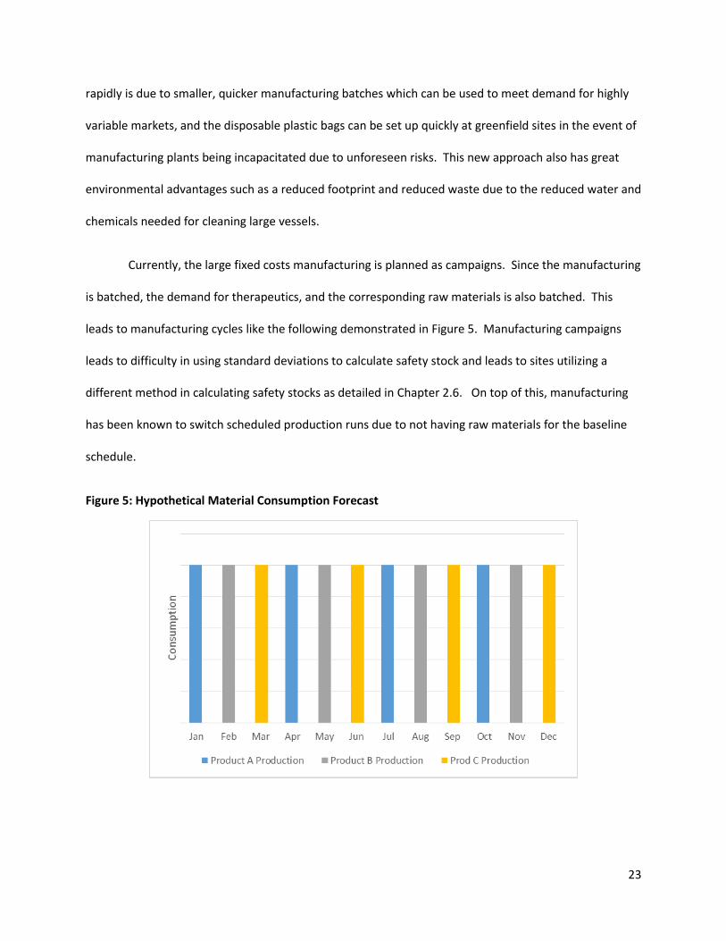
Currently, the large fixed costs manufacturing is planned as campaigns. Since the manufacturing
is batched, the demand for therapeutics, and the corresponding raw materials is also batched. This
leads to manufacturing cycles like the following demonstrated in Figure 5. Manufacturing campaigns
leads to difficulty in using standard deviations to calculate safety stock and leads to sites utilizing a
different method in calculating safety stocks as detailed in Chapter 2.6. On top of this, manufacturing
has been known to switch scheduled production runs due to not having raw materials for the baseline
schedule.
Figure 5: Hypothetical Material Consumption Forecast

24
Variable cost production relies on one therapeutic being produced with a steady, non-variable
production cycle. This deterministic manufacturing will ease the burden on the supply chain and allow
for lower levels of operational safety stock.
2.5 Warehouse Operations Overview
Amgen is a global company with global operations, and as such has a global footprint. Amgen’s
therapeutics are manufactured in 3 main manufacturing facilities and flows through 6 different
warehouses. For FY 2015 (Amgen, 2016), Amgen stored $2.4B in inventory broken out in the following:
$201M in raw material, $1.5B in work in progress, and $705M in finished therapeutics. Amgen has used
this inventory very effectively, if not efficiently, being one of two biotech companies to have never
stocked out of therapeutics to their customer.
These warehouses hold raw material, and different stages of work-in-progress and finished
therapeutics; all which have different storage temperature requirements. All warehouses have the
same basic layout and storage temperature types. The aggregated storage temperature requirements
are the following:
CRT/Ambient – This is Controlled Room Temperature/ Ambient warehouse space. This space is
used to store mostly raw materials.
2-8°C – This is cold storage warehouse space. This space is used to store mostly WIP from DP to
FDP and finished therapeutics. There are some raw materials that need to be stored in this
temperature range.
Freezers – This space is either walk in freezers, or stand – up freezers that range from -10°C to -
80°C. This is used to store mainly DS and certain DP and FDP
Haz-Mat – This is a special case of the above temperature settings where acids, bases, and
flammables must be stored in segregated areas for safety reasons
25
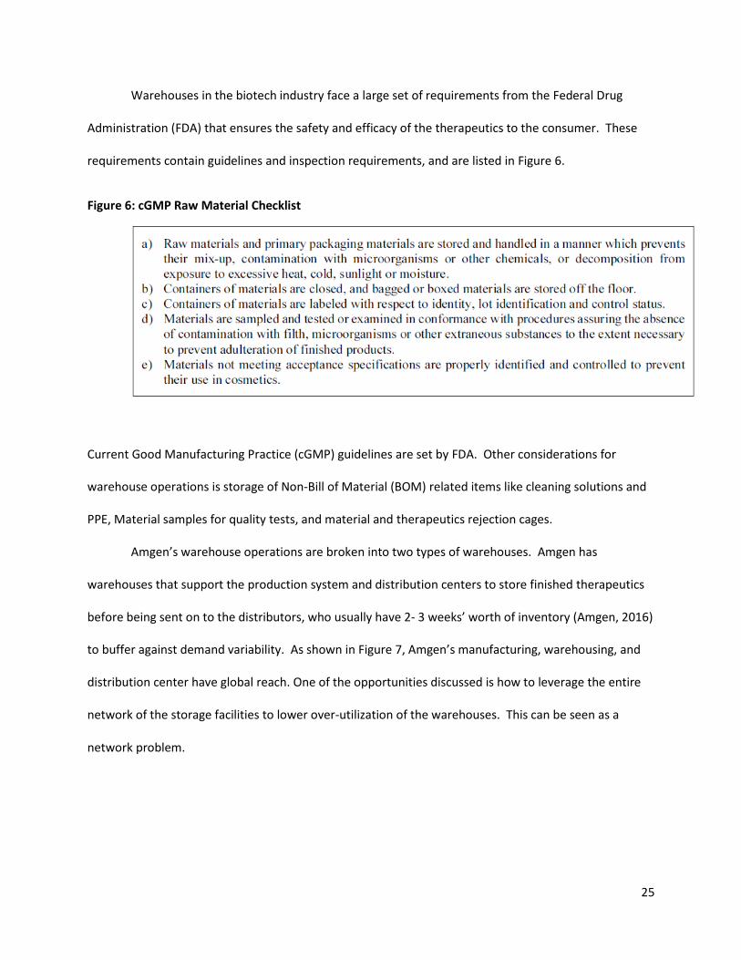
Warehouses in the biotech industry face a large set of requirements from the Federal Drug
Administration (FDA) that ensures the safety and efficacy of the therapeutics to the consumer. These
requirements contain guidelines and inspection requirements, and are listed in Figure 6.
Figure 6: cGMP Raw Material Checklist
Current Good Manufacturing Practice (cGMP) guidelines are set by FDA. Other considerations for
warehouse operations is storage of Non-Bill of Material (BOM) related items like cleaning solutions and
PPE, Material samples for quality tests, and material and therapeutics rejection cages.
Amgen’s warehouse operations are broken into two types of warehouses. Amgen has
warehouses that support the production system and distribution centers to store finished therapeutics
before being sent on to the distributors, who usually have 2- 3 weeks’ worth of inventory (Amgen, 2016)
to buffer against demand variability. As shown in Figure 7, Amgen’s manufacturing, warehousing, and
distribution center have global reach. One of the opportunities discussed is how to leverage the entire
network of the storage facilities to lower over-utilization of the warehouses. This can be seen as a
network problem.
26
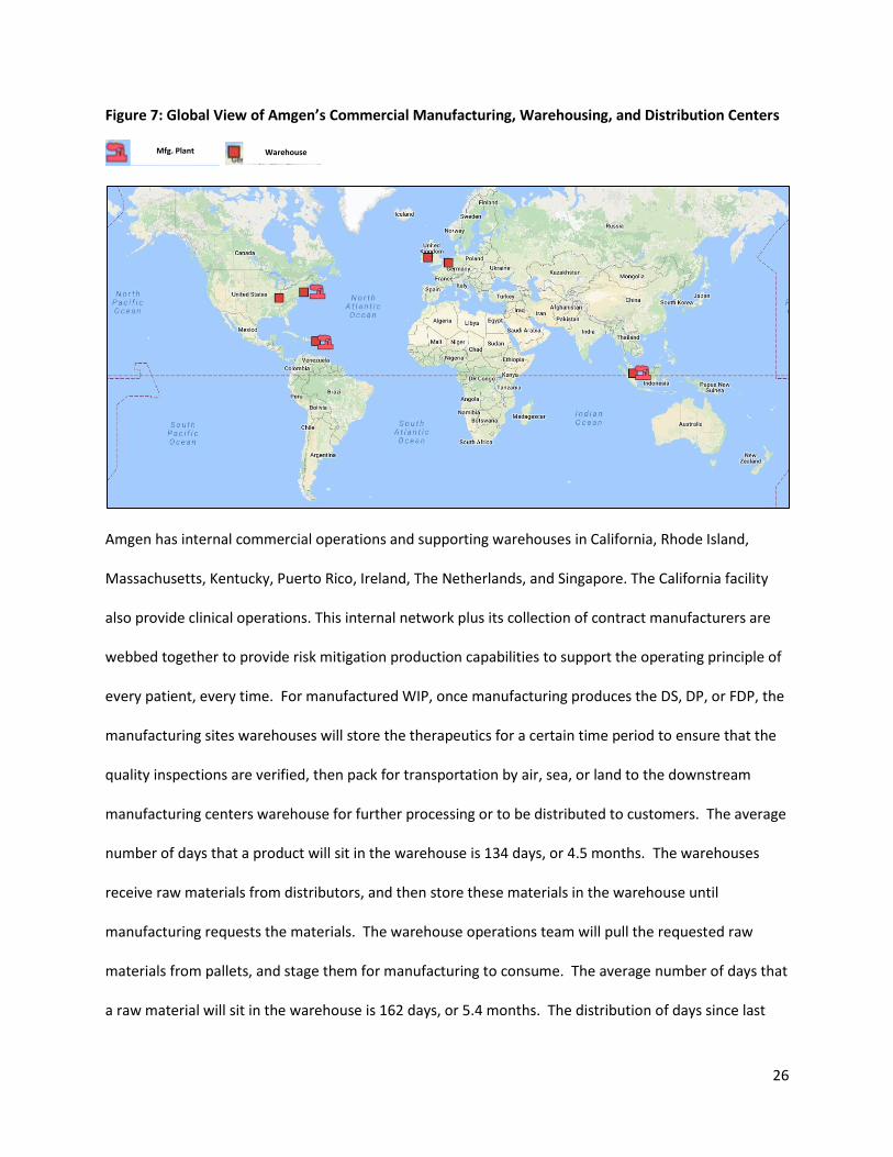
Figure 7: Global View of Amgen’s Commercial Manufacturing, Warehousing, and Distribution Centers
Amgen has internal commercial operations and supporting warehouses in California, Rhode Island,
Massachusetts, Kentucky, Puerto Rico, Ireland, The Netherlands, and Singapore. The California facility
also provide clinical operations. This internal network plus its collection of contract manufacturers are
webbed together to provide risk mitigation production capabilities to support the operating principle of
every patient, every time. For manufactured WIP, once manufacturing produces the DS, DP, or FDP, the
manufacturing sites warehouses will store the therapeutics for a certain time period to ensure that the
quality inspections are verified, then pack for transportation by air, sea, or land to the downstream
manufacturing centers warehouse for further processing or to be distributed to customers. The average
number of days that a product will sit in the warehouse is 134 days, or 4.5 months. The warehouses
receive raw materials from distributors, and then store these materials in the warehouse until
manufacturing requests the materials. The warehouse operations team will pull the requested raw
materials from pallets, and stage them for manufacturing to consume. The average number of days that
a raw material will sit in the warehouse is 162 days, or 5.4 months. The distribution of days since last
Mfg. Plant Warehouse

27
movement is shown in Figure 8. Based on this analysis, there does seem to be a decent amount of
outliers, as this distribution has very long tails. A project should be initiated to investigate if any of these
outliers really need to be in the warehouses, or could they be scrapped to open up additional capacity.
Figure 8: Distribution of Last Stock Placement (in Days) for Amgen’s Warehouses
2.6 Supply Chain Operations Overview
Amgen utilizes the following three main types of inventory: cycle stock, operational safety
stock, and strategic safety stock. Cycle stock is the average amount of inventory to meet demand
between the production cycles. Operational safety stock is inventory stored to ensure the variation of
supply and demand is met between the production cycles. Strategic safety stock is a special type of
inventory for Amgen. It is used for risk mitigation purposes, to ensure that if a manufacturing site is
unable to manufacture therapeutics due to geo-political concerns or natural disasters, the inventory will
be able to supply demand until manufacturing is restored at the affected site or delegated to an

28
alternative site to meet demand. Figure 9 demonstrates the inventory stock levels that Amgen uses for
production.
Figure 9: Amgen’s Work in Progress Inventory Levels
Cycle Stock:
This inventory is the inventory used to fulfill the anticipated demand until more can be
produced. The average cycle stock can be detailed in Equation 1.
Equation 1: Average Cycle Stock Calculation
𝐴𝑣𝑒𝑟𝑎𝑔𝑒 𝐶𝑦𝑐𝑙𝑒 𝑆𝑡𝑜𝑐𝑘 =𝑂𝑟𝑑𝑒𝑟 𝑆𝑖𝑧𝑒
2
The order size can be calculated from a given order frequency and desired production level detailed in
Equation 2.
Equation 2: Order Size Calculation
𝑶𝒓𝒅𝒆𝒓 𝑺𝒊𝒛𝒆 =𝑷𝒓𝒐𝒅𝒖𝒄𝒕𝒊𝒐𝒏 𝑹𝒂𝒕𝒆
𝑶𝒓𝒅𝒆𝒓 𝑭𝒓𝒆𝒒𝒖𝒆𝒏𝒄𝒚
29
The order frequency is the number of orders per year, and the production rate is set as the supply
required to meet the demand plus the strategic and operational safety stock.
Operational Safety Stock:
This inventory is kept on hand to manage the variability of supply and demand, along with
allocations for scrap and quality issues that could occur. The centralized raw materials team utilizes
Equation 3 to set safety stock levels. The Z value is the inverse of the cumulative standardized normal
one-tailed distribution. Currently, Amgen utilizes a 95% probability, which translates into the value of
1.64. The question is whether a 95% value is appropriate. To address this, we can draw upon the
concepts of the newsvendor problem. Given the critical fractile approach, which balances overage and
underage costs, to inventory, Amgen’s optimal safety stock inventory levels can be found. The
newsvendor model determines the service level that a company should utilize by finding the minimum
cost between underserving the market leading to lost sales, and overserving the market leading to
excess inventory and scrap. In the bio-tech industry, underserving the market could lead to much graver
situations, including market backlash, loss of reputation for other products, accelerated regulatory
approval of competitor products, and up to patient’s death, hence the philosophy of ensuring “every
patient, every time”. Analysis of Amgen’s optimal service level based on the newsvendor problem was
found to be 99% (Yang, 2015). Based on this analysis, Amgen is using the incorrect service level of 95%,
but due to the site supply chain managers ordering more safety stock then prescribed, it is unclear
whether the correct safety stock is being held. Manufacturing has been known to switch scheduled
production runs due to not having raw materials for the baseline schedule.
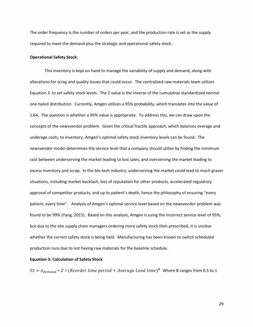
Equation 3: Calculation of Safety Stock
𝑆𝑆 = 𝜎𝑑𝑒𝑚𝑎𝑛𝑑 ∗ 𝑍 ∗ (𝑅𝑒𝑜𝑟𝑑𝑒𝑟 𝑡𝑖𝑚𝑒 𝑝𝑒𝑟𝑖𝑜𝑑 + 𝐴𝑣𝑒𝑟𝑎𝑔𝑒 𝐿𝑒𝑎𝑑 𝑡𝑖𝑚𝑒)𝐵 Where B ranges from 0.5 to 1

30
The B in this equation is based on risk-pooling theory and is described in more detail in Chapter
3. Reflecting on the operations philosophy of serving “every patient, every time”, and the newsvendor
model results, manufacturing sites supply chain managers utilize safety stock to cover the most that
could be needed, and usually does not consider the typical probabilistic approach dictated in Equation 3.
Factors that influence the site supply chain managers’ decisions are sourcing diversification,
ease of sourcing, supplier financial health, and a history of supply disruptions. At Amgen, safety stock is
combined with cycle stock and treated as a variable that could be known as Months on Hand (MOH) of
inventory. This is basically a blanket setting to ensure that there is enough raw material inventory on
hand for X months of production.
Strategic Safety Stock:
To calculate strategic safety stock inventory, a risk team calculates the probability of an event
that would incapacitate the manufacturing plant; whether it be fire, flood, storm, geo-political, or other
disaster. The time period until production can be restored at that site, or another site, is calculated
from the time the event occurs to the time manufacturing capacity can be restored. The amount of
inventory to ensure that the demand is met during that time period is calculated as months of forward
coverage, or MFC. This inventory is stored for every stage of therapeutics work in progress from DS to
FDP detailed in the above section, and is not to be utilized except for risk mitigation purposes. A project
should be explored for understanding the Time to Survive (TTS) for each manufacturing plant and
compared to the Time to Failure (TTF) to ensure TTS>TTF. This idea is explored in Chapter 3.
Amgen’s lead times for raw materials is widely variable, and with a median lead time of 61 days
and an average lead time of 63 days. The distribution of lead times for raw materials is shown in Figure
10.

31
Figure 10: Distribution of frequency of lead time (in days) of raw materials
Based on this, significant opportunities do abound to reduce lead times, and correspondingly, safety
stock levels at warehouses. This analysis is explained in Chapter 3.
2.7 Long Range Plan Overview
Amgen’s LRP is created by the sales and marketing organization in conjunction with the supply
chain organization. This plan is updated multiple times throughout the year when new information is
made available, such as new market opportunities or current commercial therapeutics are allowed to be
marketed to new indications. It is important to note that no forecast error is created for successive
iterations of the LRP. With a proper forecast error, scientific formulas for inventory could be created
and utilized to better ensure “every patient, every time”.
The following bullets detail how each portion of the LRP is calculated:
Demand - Marketing and supply chain managers build a ten year annual forecast of all customer
demand from the different markets of each therapeutic over the next ten years. This is

32
aggregated for each manufacturing site and therapeutics and its respective demand for a given
year.
Supply - Operations calculates the downstream supply (i.e. in order to make 1,000 FDP, it
requires X DP units and Y DS lots ) required to make the final therapeutics to ensure demand is
met plus a projected balance for risk mitigation, lead times, and anticipated scrap. This is
aggregated from the separate markets for each manufacturing site based on its respective
supply for a given year.
Projected Balance - The projected balance is the amount of therapeutics that will be stored to
ensure the variation of demand is met and provide risk mitigation of unforeseen events. This is
detailed in Equation 4.
Equation 4: Calculation of Projected Balance
𝑃𝑟𝑜𝑗𝑒𝑐𝑡𝑒𝑑 𝐵𝑎𝑙𝑎𝑛𝑐𝑒𝑌𝑒𝑎𝑟 = 𝑃𝑟𝑜𝑗𝑒𝑐𝑡𝑒𝑑 𝐵𝑎𝑙𝑎𝑛𝑐𝑒𝑌𝑒𝑎𝑟−1 + 𝑆𝑢𝑝𝑝𝑙𝑦𝑌𝑒𝑎𝑟 − 𝐷𝑒𝑚𝑎𝑛𝑑𝑌𝑒𝑎𝑟

33
3 Literature Review
Research is to see what everybody else has seen, and to think what nobody else has thought.
-Albert Szent-Gyorgyi
Prior to and during the development of the warehouse strategy, and corresponding model to
support the strategy, much effort was expended to research the existing approaches. We will start with
research close to Amgen’s operations, then discuss the broader literature available to support a robust
solution to the problem statement.
3.1 Amgen’s Operations in Literature
Two warehouse models have already been detailed from previous MIT Leaders for Global
Operations program thesis. Jason Choi in “Raw Material Inventory Planning in a Serial System with
Warehouse Capacity” (Choi, 2014) discusses the inventory management policies and corresponding
warehouse capacity required for one warehouse at Amgen. To reduce inventory at that warehouse and
gain additional capacity, Choi recommends the following:
Batch size optimization based on available warehouse space
Safety stock reduction due to removal of demand variability by fixing the production system
Reduce Stock Keeping Units (SKU) complexity through commonality of raw materials, which will
lead to lower levels of safety stock
Utilize Vendor Managed Inventory (VMI) to reduce inventory
Utilize 3rd party logistics (3PL) in series to minimize warehouse transfers
Maxine Yang realizes in “Optimization of Warehouse Operations and Transport Risk Mitigation
for Disposable Bioreactor Bags to Support Launch of Amgen Singapore Manufacturing” (Yang, 2015) the
significant amount of safety stock being held at a specific warehouse, forecast changes that increased
the demand, and how Bill of Material (BOM) changes affected storage capacity. She then proposes an
excel-based model that will calculate the storage requirements based on lot production rates,
34
capacities, efficiencies, and forward coverage (safety stock levels). Her model calculated warehouse
over-utilization in the near future, and recommended the following steps to reduce overutilization.
Store raw material inventory at supplier’s warehouses
Reduce lead time of raw materials
Increase raw material delivery frequency
Random assignments of pallet spaces
Utilization of 3PL to store materials
Reduce testing and release times for raw materials
According to the World Bank (Unknown, The World Bank, 2016), the average time to build a
warehouse is 160 days. This is widely variable across countries. An internal study (Unknown, 2007) at
Amgen revealed the average fixed cost to build a warehouse is around $29M, with an average fixed cost
per pallet location space is around $5,000 with a standard deviation of $2,700. Warehouses are capital
intensive cost centers, and therefore are not readily invested in unless truly needed.
3.2 Broader Themes in Literature relevant to this case
When building a prediction model, a good starting point should be Daniel Kahneman’s and Amos
Tversky’s, “On the Psychology of Prediction” (Tversky, 1973). They summarize that the best way to
create a prediction is to perform the following steps:
1) Understand the prior information, or base rate.
2) Understand the specific evidence about the base case.
3) Determine the expected accuracy, or range, of the prediction.
Given this understanding, it’s important to understand the current state, the equations driving
the current state, and for the predictor to give a knowledgeable range of the prediction to ensure a
proper model. Tversky and Kahneman describe how graduate students were given information about a
person who scored on the 99th percentile on an IQ test, but the test had a known error. The students
were asked to estimate a range of the true IQ score. The students gave an interval that was equal

35
around the 99th percentile, not realizing that the average score was at the 50th percentile. Therefore,
the range should have been a heavily tilted toward the base rate. This type of bias leads to faulty
models.
Sean Willems states in his paper, “Demystifying Inventory” (Willems, 2015) that using metrics
such as MOH are wrong.
“That is, the [MOH] is calculated by determining how many [Months] into the future existing inventory on hand can satisfy. This corporate metric, which has some value, reinforces the incorrect intuition to focus on forward-looking parameters when setting inventory targets. So while we have definitively shown that forward [Months] of coverage is a bad metric to use for inventory planning purposes, its value as a corporate metric reinforces its incorrect usages for safety stock target setting.”
He further states the hardest step in optimizing inventory across the end-to-end supply chain is moving
from ad hoc unscientific MOH to a scientifically derived inventory targets. He recommends moving
from the 1st frontier to a 3rd frontier of inventory optimization:
1) Ad Hoc “Heuristics” Inventory Policies
2) Single Stage Scientifically Calculated Inventory Policies
3) Multi-Echelon Inventory Policies
The implication of these stages are detailed in Figure 11.

36
Figure 11: The Three Frontiers of Inventory Optimization (Willems, 2015)
Proper inventory levels have been detailed heavily in operations, and one of the more
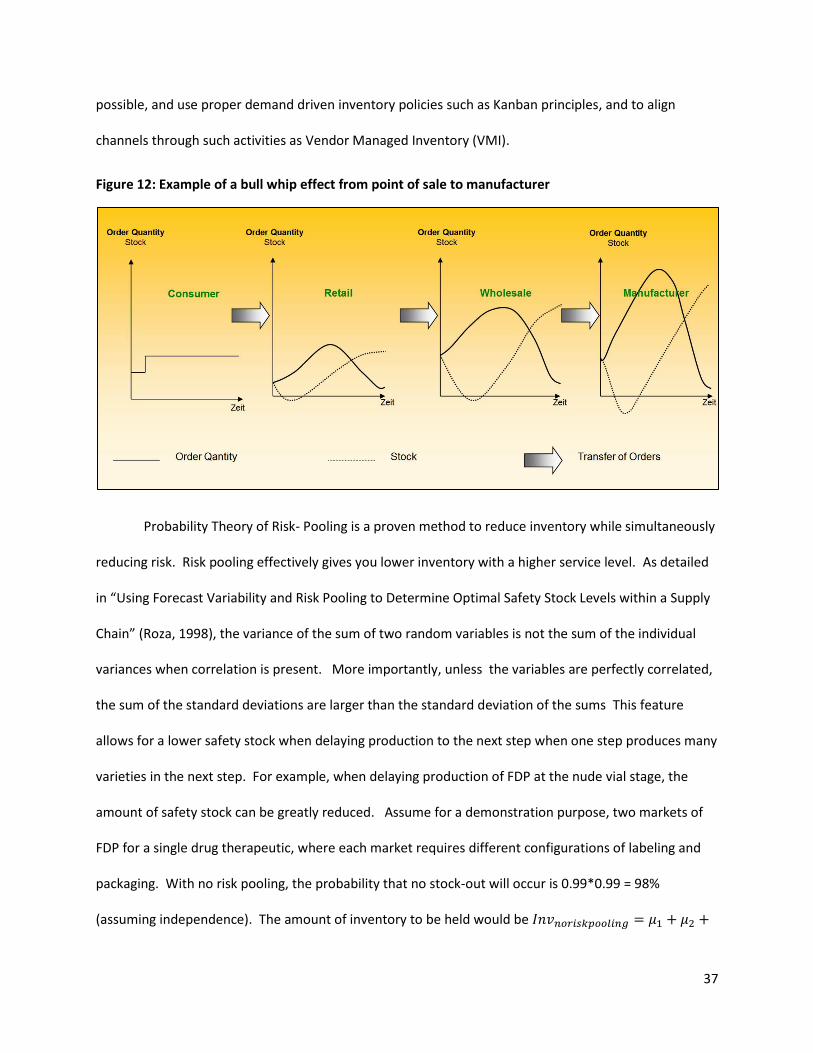
frequently studied issues is the bull whip effect. The bull whip effect is due to variations in demand
travelling upstream in the distribution system. This leads to increases in variation at each step in the
supply chain, leading to large swings at the source. Research indicates a fluctuation in demand of +/- 5%
at the point of sale can lead to a +/- 40% change in demand at the source (Hau L. Lee, 1997). This can be
pictured in Figure 12 to showcase how small changes in demand propagate through the supply chain.
The consequence of this typically leads to either stock-outs or excessive inventory. To counteract this
problem, it’s necessary to extend the visibility of customer demand as far back in the supply chain as
37
possible, and use proper demand driven inventory policies such as Kanban principles, and to align
channels through such activities as Vendor Managed Inventory (VMI).
Figure 12: Example of a bull whip effect from point of sale to manufacturer
Probability Theory of Risk- Pooling is a proven method to reduce inventory while simultaneously
reducing risk. Risk pooling effectively gives you lower inventory with a higher service level. As detailed
in “Using Forecast Variability and Risk Pooling to Determine Optimal Safety Stock Levels within a Supply
Chain” (Roza, 1998), the variance of the sum of two random variables is not the sum of the individual
variances when correlation is present. More importantly, unless the variables are perfectly correlated,
the sum of the standard deviations are larger than the standard deviation of the sums This feature
allows for a lower safety stock when delaying production to the next step when one step produces many
varieties in the next step. For example, when delaying production of FDP at the nude vial stage, the
amount of safety stock can be greatly reduced. Assume for a demonstration purpose, two markets of
FDP for a single drug therapeutic, where each market requires different configurations of labeling and
packaging. With no risk pooling, the probability that no stock-out will occur is 0.99*0.99 = 98%
(assuming independence). The amount of inventory to be held would be 𝐼𝑛𝑣𝑛𝑜𝑟𝑖𝑠𝑘𝑝𝑜𝑜𝑙𝑖𝑛𝑔 = 𝜇1 + 𝜇2 +

38
𝑍(𝜎1 + 𝜎2) ∗ √𝑟 + 𝑙 . With risk pooling, the probability of meeting demand with the each therapeutics
inventory is 99%, and the amount of inventory to be held would be 𝐼𝑛𝑣𝑅𝑖𝑠𝑘𝑝𝑜𝑜𝑙𝑖𝑛𝑔 = 𝜇1 + 𝜇2 + 𝑍(𝜎𝑇) ∗
√𝑟 + 𝑙 where 𝜎𝑇 = √𝜎12 + 𝜎2
2 + 2𝜌12𝜎1𝜎2, and 𝜌12 is the correlation value between the demand of 1
and 2. Given the ranges of 1 to -1 for 𝜌12, the safety stock can range from a worst case of 𝜎𝑇 = 𝜎1 + 𝜎2
when 𝜌12 = 1 to the best case of 𝜎𝑇 = 𝜎1 − 𝜎2 when 𝜌12= -1.
To understand the base case of inventory, an inventory model should understand how product
demand is built up. Rosenfield states, (Rosenfield, 2014)
“The driver of inventory is forecast error. If forecast error is high, then more inventories is required to address the uncertainties. To establish how inventory varies, [an] analysis of three types of relationships should be studied:
The relationship between inventory and forecast error
The relationship between forecast error and the lead time over which it is calculated
The relationship between forecast error and product volume First, inventory increases as forecast error increases, because reserve
stocks or safety stocks are generally proportional to the magnitude of
forecast error. Because reserve stocks or safety stocks are typically the
predominant part of inventory, we assume that inventories will behave
as reserve stocks behave and thus be proportional to the magnitude of
the forecast error. We can thus use standard inventory models for
safety or reserve stocks”
Rosenfield further states that the “variance of the demand forecast is proportional to the average total
demand. Hence the square root of the variance, the standard deviation, is proportional to the square
root of the average total demand.” (Rosenfield, 2014) This leads to the same result of the equation
detailed in the above paragraph. Not only does this mean that demand forecast should be
proportional, but also that lead times should be proportional. Although these two relationships do not
always follow a square root relationship, there is a concave relationship between demand variation and
forecast error and lead times, which is due to correlations of these two variables. These concave
39
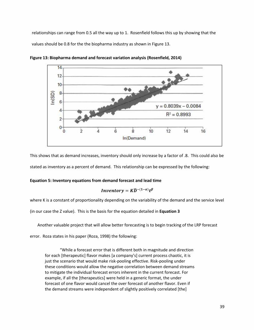
relationships can range from 0.5 all the way up to 1. Rosenfield follows this up by showing that the
values should be 0.8 for the the biopharma industry as shown in Figure 13.
Figure 13: Biopharma demand and forecast variation analysis (Rosenfield, 2014)
This shows that as demand increases, inventory should only increase by a factor of .8. This could also be
stated as inventory as a percent of demand. This relationship can be expressed by the following:
Equation 5: Inventory equations from demand forecast and lead time
𝑰𝒏𝒗𝒆𝒏𝒕𝒐𝒓𝒚 = 𝑲�̅�−(𝟏−𝜶)𝒕𝜷
where K is a constant of proportionality depending on the variability of the demand and the service level
(in our case the Z value). This is the basis for the equation detailed in Equation 3
Another valuable project that will allow better forecasting is to begin tracking of the LRP forecast
error. Roza states in his paper (Roza, 1998) the following:
“While a forecast error that is different both in magnitude and direction for each [therapeutic] flavor makes [a company’s] current process chaotic, it is just the scenario that would make risk-pooling effective. Risk-pooling under these conditions would allow the negative correlation between demand streams to mitigate the individual forecast errors inherent in the current forecast. For example, if all the [therapeutics] were held in a generic format, the under forecast of one flavor would cancel the over forecast of another flavor. Even if the demand streams were independent of slightly positively correlated [the]
40
sheer aggregation tends to decrease total variability and thus the required safety stock.”
Lead time reductions also offer lower inventory levels and increased flexibility without any
additional risk. This can be accomplished with better inventory management policies like implementing
Kanban systems. With shorter lead times, production can choose to delay shipment of items they do
not need until later if the production schedule needs to be shifted, providing flexibility. Shorter lead
times also decreases the time an item is not exposed to risks in shipments. Given the calculation for
safety stock levels in Equation 3, the equation for determining the safety stock reduction through lead
time reduction is listed in Equation 6.
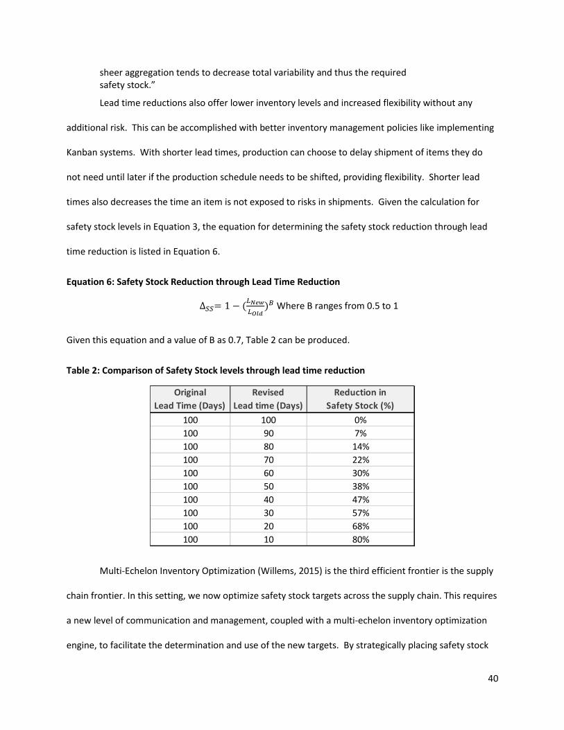
Equation 6: Safety Stock Reduction through Lead Time Reduction
∆𝑆𝑆= 1 − (𝐿𝑁𝑒𝑤
𝐿𝑂𝑙𝑑)𝐵 Where B ranges from 0.5 to 1
Given this equation and a value of B as 0.7, Table 2 can be produced.
Table 2: Comparison of Safety Stock levels through lead time reduction
Multi-Echelon Inventory Optimization (Willems, 2015) is the third efficient frontier is the supply
chain frontier. In this setting, we now optimize safety stock targets across the supply chain. This requires
a new level of communication and management, coupled with a multi-echelon inventory optimization
engine, to facilitate the determination and use of the new targets. By strategically placing safety stock
Original
Lead Time (Days)
Revised
Lead time (Days)
Reduction in
Safety Stock (%)
100 100 0%
100 90 7%
100 80 14%
100 70 22%
100 60 30%
100 50 38%
100 40 47%
100 30 57%
100 20 68%
100 10 80%

41
inventory in the supply chain nodes, safety stock could be reduced at other nodes due to the lead time
of the safety stock being able to bridge the needs of the following nodes. This is best accomplished by
decoupling safety stock before a major value add step of manufacturing where the product is relatively
cheap, and removing safety stock at the following levels until safety stock is held for the customer. The
mathematical basis of reducing inventory through multi-echelon inventory optimization is the same as
risk pooling in the previous paragraphs on risk pooling, but instead of optimizing two stages of the
supply chain, MEIO minimizes costs across the entire supply chain while still ensuring “every patient,
every time”.
For the optimization of inventory in a multi-echelon system, the following optimization program
should be used (Sean Willems, 2011):
𝑷 min ∑ 𝑐𝑗(𝑆𝐼𝑗,𝑆𝑗)
|𝑁|
𝑗=1
𝒔. 𝒕. 𝑆𝑗 − 𝑆𝐼𝑗 ≤ 𝑇𝑗 ∀𝑗∈ 𝑁
𝑆𝐼𝑗 − 𝑆𝑗 ≥ 0 ∀(𝑖, 𝑗) ∈ 𝐴
𝑆𝑗 ≤ 𝑠𝑗 ∀𝑗: ∄𝑘 ∈ 𝑁| (𝑗, 𝑘) ∈ 𝐴
𝑆𝑗, 𝑆𝐼𝑗 ≥ 0, 𝑖𝑛𝑡𝑒𝑔𝑟𝑎𝑙 ∀𝑗∈ 𝑁
Where 𝑇𝑗 is the time required to complete the processing requirements of stage 𝑗, 𝑆𝐼𝑗 is the longest
outgoing service time from upstream adjacent stages quoted to stage 𝑗, 𝑆𝑗 is the delivery time stage 𝑗
quotes its adjacent downstream stages, and 𝑠𝑗 𝑖𝑠 𝑡ℎ𝑒 𝑚𝑎𝑥𝑖𝑚𝑢𝑚 𝑜𝑢𝑡𝑔𝑜𝑖𝑛𝑔 𝑠𝑒𝑟𝑣𝑖𝑐𝑒 𝑡𝑖𝑚𝑒 𝑎𝑡 𝑠𝑡𝑎𝑔𝑒 𝑗.
Each stage has a cost function𝑐𝑗(𝑆𝐼𝑗,𝑆𝑗) which is a function of its incoming and outgoing service times,
and is the costs of holding inventory at the stage.
The objection function minimizes the total stage cost. The first constraint ensures the outgoing
service level for each node is below the quoted service time plus its own lead time. The second
constraint ensures the incoming service level for each node to be at least as large as the longest
outgoing service time quoted to the node. The third constraint enforces an upper bound on a demand
nodes outgoing service time. The final constraints require service times to be nonnegative and integer.
42
Time to Survive (TTS) analysis could be used to right-size the strategic safety stock levels at
Amgen (Simchi-Levi, 2010). Amgen has already analyzed and found the Time to Recovery analysis,
which is the time it takes to recover manufacturing capacity after an unforeseen disaster to its supply
chain. TTS represents the time a supply chain system can continue to operate while its sources of supply
are disrupted. Instead of focusing and holding a strategic safety stock, Amgen could perform a study on
the TTS of its supply chain, and as long as TTS> TTR, the strategic inventory above that mark could be
reduced. This exercise could also be used to identify risks to the supply chain.
4 Methodology
4.1 Current State Analysis
Amgen’s current warehouse strategy is reactive, with each warehouse site director managing
their individual warehouse capacity, with therapeutic supply chain managers flowing their respective
therapeutics through specific warehouses. This is all done with limited communication among
warehouses, reactive decisions to add capacity, no common tools among the warehouses to study
improvements to capacity, and with little consideration of the network. This leads to network
inefficiencies, with some warehouses being over utilized, resulting in costly 3rd party storage, while other
warehouses are run at low capacities, meaning low economies of scale, especially for cold storage.
An existing warehouse capacity utilization model has been constructed for each individual
warehouse on a rolling month to month 24 month forward looking basis. Amgen’s Operations Strategy
Planning & Risk (OSPR) group created these models, and updates these models monthly based on new
planning updates. OSPR has reached out to train each warehouse site to run the model, but the model
complexity is a labor intensive, technically complex spreadsheet that most warehouse site personnel do
not have the time to understand the complexity driving the model. The models are used by the sites to
43
help understand the capacity utilization of individual sites. Each site has a representative that works
with the site director to ensure the model reflects reality, and is used to plan capacity upgrades.
4.2 Baseline Warehouse Capacity Model Creation
A model is a lie that helps you see the truth – Howard Skipper
In order to create a strategy for Amgen’s warehouse network, the networks capacity needs must
be understood over the time period in question. In order to fulfill this need, a model was constructed to
understand the capacity requirements over an 8 year period, understand what is driving the capacity,
and understand the different scenarios to alleviate capacity overutilization. Chapter 4.2 will detail the
baseline model creation through its inputs, queries, and outputs, along with the simulation of different
scenarios for business case evaluation. The model was chosen to be created in Microsoft Access®, a
relational database tool that allows large streams of data to be linked together for custom reports.
Access was utilized due to the ease of use, ease of access (as this project was over a six month period,
speed was essential), and its ability to integrate with other Microsoft Office tools such as Excel® which
the OSPR group is more readily experienced in.
4.2.1 Model Inputs
The Baseline Warehouse Capacity model utilizes tables that were either variables that the model
builder can update, or constants that come from planning. The following are tables with either a (V) to
label it as a table that contains variables, or a (C) to label it as a table full of constants. The variable
tables can be updated by the user to provide scenario based model runs. I.e. what would happen if each
site warehouses would increase their pallet utilization to 85%?
Site Planning Tables (C) – These tables (1 table for each site) are from the LRP detailed in
Chapter 2.7. They contain the total demand for each site therapeutics by therapeutics by year, the
44
supply by therapeutics being manufactured at that site for each year, and the projected balance being
held on site each year1.
BOMs (C) – This table is the Bill of Materials (BOMs) for each therapeutics. This provides the
raw materials required with the quantity in order to make each therapeutics by site. This table also
contains a normalized quantity of the required amount of raw materials required to make therapeutics.
(i.e. In order to make 1,000 FDP units of Therapeutics A, utilize 2,000 of raw material A.)
Material Master (C) – This table provides the temperature requirements for every raw material
and therapeutics, and the quantity of material or therapeutics that makes up a pallet.
Warehouse Capacity and Pallet Utilization – This table provides the pallet utilization (V) and
capacity (C) of each warehouse by temperature storage type. The pallet utilization table details how
efficient the warehouses are at storing pallets at an aggregate level. i.e. If a pallet space can hold 10
filters, but only 5 filters are stored there, the pallet utilization is 50%. Each warehouse provided its own
pallet utilization that it calculated over the past six months by temperature storage type.
Months on hand (V) – This table is the months on hand (MOH) of raw material and therapeutics
aggregated by material sub-group (i.e chemicals, excipients, filters…) or therapeutics by months on hand
for each site. As detailed in Chapter 2.6, this is a combination of cycle stock and safety stock. As even
sites supply chain managers do not use the standard equations to determine inventory levels, a formula
was calculated to approximate the MOH. These values were calculated by comparing the average
inventory on hand over time (minimum 6 months) to the supply required for that year by site. This
calculation is detailed in Equation 7. The 𝐴𝑣𝑒𝑟𝑎𝑔𝑒(𝐴𝑐𝑡𝑢𝑎𝑙 𝑝𝑎𝑙𝑙𝑒𝑡𝑠 𝑜𝑛 ℎ𝑎𝑛𝑑𝑀𝑎𝑡𝑙_𝑆𝑢𝑏_𝐺𝑟𝑜𝑢𝑝) was found
from the short term model for the 24 month period for each Matl_Sub_Group.
1 Note: Due to 2016 being 75% of the way done in October 2016, the 2016 year’s balance is only 25% of the
annual. This leads to some interesting results for year 2016. The models output should only be considered for years 2017 onwards.

45
Equation 7: Months on Hand Calculation
𝑀𝑜𝑛𝑡ℎ𝑠 𝑜𝑛 𝐻𝑎𝑛𝑑𝑀𝑎𝑡𝑙_𝑆𝑢𝑏_𝐺𝑟𝑜𝑢𝑝 =𝐴𝑣𝑒𝑟𝑎𝑔𝑒(𝐴𝑐𝑡𝑢𝑎𝑙 𝑝𝑎𝑙𝑙𝑒𝑡𝑠 𝑜𝑛 ℎ𝑎𝑛𝑑𝑀𝑎𝑡𝑙_𝑆𝑢𝑏_𝐺𝑟𝑜𝑢𝑝)
(𝑃𝑎𝑙𝑙𝑒𝑡𝑠 𝑟𝑒𝑞𝑢𝑖𝑟𝑒𝑑 𝑡𝑜 𝑚𝑒𝑒𝑡 𝑎𝑛𝑛𝑢𝑎𝑙 𝑆𝑢𝑝𝑝𝑙𝑦/12)
Manual Updates (V) – This table is a catch all table used to allocate any non-BOM materials by
year i.e. PPE, Shipping Containers, Quality Samples, and any other pallet space quantities that are word
of mouth. To calculate the manual updates, the team worked with sites and future forecasts to find the
average amount of pallets needed to allocate to warehouses over the next 8 years. This also included
pipeline therapeutics that did not have BOM’s for the raw materials needs. To calculate this, the
demand for the pipeline therapeutics was compared to a similar therapeutics with a known BOM, and
the ratio of demands and raw materials MOH’s was used to find the unknown pallet spaces as detailed
in Equation 8.
Equation 8: Calculations of Pallet spaces required for Pipeline Therapeutics with no known BOM’s
𝐷𝑒𝑚𝑎𝑛𝑑𝑃𝑖𝑝𝑒𝑙𝑖𝑛𝑒
𝐷𝑒𝑚𝑎𝑛𝑑𝑆𝑖𝑚𝑖𝑙𝑎𝑟𝑃𝑟𝑜𝑑𝑢𝑐𝑡=
𝑃𝑎𝑙𝑙𝑒𝑡 𝑆𝑝𝑎𝑐𝑒𝑠 𝑅𝑒𝑞𝑢𝑖𝑟𝑒𝑑𝑃𝑖𝑝𝑒𝑙𝑖𝑛𝑒
𝑃𝑎𝑙𝑙𝑒𝑡 𝑆𝑝𝑎𝑐𝑒𝑠 𝑅𝑒𝑞𝑢𝑖𝑟𝑒𝑑𝑆𝑖𝑚𝑖𝑙𝑎𝑟𝑃𝑟𝑜𝑑𝑢𝑐𝑡
4.2.2 Model Queries
There were over 30 queries created for this model due to the complexity of the BOM’s, detailing
the inventory types, and creating custom reports based on customer requests. The following will be
high level queries to determine the different types of inventory. Many sub-queries were created to
filter out certain items for further processing or the author lacked the knowledge of how to simplify the
queries.
Projected Balance – The projected balance of therapeutics to be stored at each site annually
was converted to pallet quantities and matched with the storage temperature requirements as detailed
in Equation 9.
Equation 9: Pallets of Projected Balance

46
𝑃𝑎𝑙𝑙𝑒𝑡𝑠 𝑜𝑓 𝑃𝑟𝑜𝑗𝑒𝑐𝑡𝑒𝑑 𝐵𝑎𝑙𝑎𝑛𝑐𝑒𝑝𝑟𝑜𝑑𝑢𝑐𝑡 𝑠𝑖𝑡𝑒 𝑦𝑒𝑎𝑟 =𝑃𝑟𝑜𝑗𝑒𝑐𝑡𝑒𝑑 𝐵𝑎𝑙𝑎𝑐𝑛𝑒𝑝𝑟𝑜𝑑𝑢𝑐𝑡 𝑠𝑖𝑡𝑒 𝑦𝑒𝑎𝑟
(𝑄𝑢𝑎𝑛𝑖𝑡𝑦 𝑝𝑒𝑟 𝑃𝑎𝑙𝑙𝑒𝑡)
Raw Materials – This section of the model utilized 18 queries to pull together all the raw
materials required to be on hand to support the supply dictated from the LRP. The queries filter the LRP
for the quantity to be manufactured (supplied) by product by site for a given year and determines the
raw materials required to make that supply. This value is then multiplied by the MOH for each material
sub group, and then divided by the quantity per pallet for each raw material. This is captured in
Equation 102.
Equation 10: Calculation of Raw Material
𝑃𝑎𝑙𝑙𝑒𝑡𝑠 𝑜𝑓 𝑋 𝑅𝑎𝑤 𝑀𝑎𝑡𝑒𝑟𝑖𝑎𝑙𝑖𝑡𝑒𝑚 𝑠𝑖𝑡𝑒 𝑦𝑒𝑎𝑟 = 𝑖𝑛𝑡𝑒𝑔𝑒𝑟(𝑆𝑢𝑝𝑝𝑙𝑦 𝑅𝑒𝑞𝑢𝑖𝑟𝑒𝑑𝑖𝑡𝑒𝑚 𝑠𝑖𝑡𝑒 𝑦𝑒𝑎𝑟 ∗
𝑀𝑜𝑛𝑡ℎ𝑠 𝑜𝑛 𝐻𝑎𝑛𝑑12
𝑄𝑢𝑎𝑛𝑡𝑖𝑡𝑦 𝑝𝑒𝑟 𝑃𝑎𝑙𝑙𝑒𝑡)
Work in Progress – This section of the model determines the Work in Progress for each site.
The time it takes from when a therapeutics is manufactured, stored at that manufacturing sites
warehouse then shipped to the downstream manufacturing site’s warehouse before it is processed into
its next steps.
Equation 11: Calculation of WIP Inventory
𝑃𝑎𝑙𝑙𝑒𝑡𝑠 𝑜𝑓 𝑋 𝑊𝐼𝑃𝑝𝑟𝑜𝑑𝑢𝑐𝑡 𝑠𝑖𝑡𝑒 𝒚𝒆𝒂𝒓 = 𝑖𝑛𝑡𝑒𝑔𝑒𝑟 ((𝑆𝑢𝑝𝑝𝑙𝑦 𝑅𝑒𝑞𝑢𝑖𝑟𝑒𝑑𝑖𝑡𝑒𝑚 𝑠𝑖𝑡𝑒 𝒚𝒆𝒂𝒓 )∗
𝑀𝑜𝑛𝑡ℎ𝑠 𝑜𝑛 𝐻𝑎𝑛𝑑
12
𝑄𝑢𝑎𝑛𝑡𝑖𝑡𝑦 𝑝𝑒𝑟 𝑃𝑎𝑙𝑙𝑒𝑡)
4.2.3 Model Outputs
Total Storage Requirements – This combines the above queries plus the manual updates into
one table. It also adjusts every pallet by the efficiency as detailed in Equation 12. This is each sites’
pallet storage needs by temperature requirement over the next 8 years.
2 Note: Some queries had to filter out and convert kgs and liters of raw material ingredients into the material
storage units of grams and milliliters by multiplying the amount by 1000

47
Equation 12: Pallet Efficiency3
𝐴𝑑𝑗𝑢𝑠𝑡𝑒𝑑 𝑃𝑎𝑙𝑙𝑒𝑡 𝑄𝑢𝑎𝑛𝑡𝑖𝑡𝑦 = 𝑃𝑎𝑙𝑙𝑒𝑡 𝑄𝑢𝑎𝑛𝑡𝑖𝑡𝑦/𝐸𝑓𝑓𝑖𝑐𝑖𝑒𝑛𝑐𝑦
Warehouse Capacity Utilization – This is the aggregated capacity utilization for each site and
temperature requirement over 8 years by year. This is the summation of the adjusted pallet quantity
divided by the capacity of that site as detailed in Equation 13.
Equation 13: Warehouse Capacity Utilization
𝑊𝑎𝑟𝑒ℎ𝑜𝑢𝑠𝑒 𝐶𝑎𝑝𝑎𝑐𝑖𝑡𝑦 𝑈𝑡𝑖𝑙𝑖𝑧𝑎𝑡𝑖𝑜𝑛𝑠𝑖𝑡𝑒 𝑡𝑒𝑚𝑝 𝑦𝑒𝑎𝑟 =𝑆𝑢𝑚(𝐴𝑑𝑗𝑢𝑠𝑡𝑒𝑑 𝑃𝑎𝑙𝑙𝑒𝑡 𝑄𝑢𝑎𝑛𝑡𝑖𝑡𝑦𝑠𝑖𝑡𝑒 𝑡𝑒𝑚𝑝 𝑦𝑒𝑎𝑟)
𝐶𝑎𝑝𝑎𝑐𝑖𝑡𝑦𝑠𝑖𝑡𝑒 𝑡𝑒𝑚𝑝
After compiling the results of the models, the summation of the pallets over capacity will be
calculated for all warehouses. This will be used to showcase the over utilization changes in the network
capacity. This equation is detailed in Equation 14: Pallets over Capacity summation
Equation 14: Pallets over Capacity summation
𝑃𝑎𝑙𝑙𝑒𝑡𝑠 𝑂𝑣𝑒𝑟 𝐶𝑎𝑝𝑎𝑐𝑖𝑡𝑦_𝑦𝑒𝑎𝑟 = ∑ 𝑃𝑎𝑙𝑙𝑒𝑡𝑠 𝑜𝑣𝑒𝑟 𝑐𝑎𝑝𝑎𝑐𝑖𝑡𝑦𝑖
𝑤𝑎𝑟𝑒ℎ𝑜𝑢𝑠𝑒 𝑖=𝑛
𝑤𝑎𝑟𝑒ℎ𝑜𝑢𝑠𝑒 𝑖=0
To compare the overutilization effects to the costs of building extra capacity at a site to support
the capacity needs, each warehouse secured bids for the costs to move a pallet from its warehouse to
store it at 3PL. The costs were multiplied by the number of pallets needing to be stored at the 3PLs to
give a financial picture of the decision of how to add capacity. This equation is detailed in Equation 15.
Equation 15: 3PL Cost for adding additional capacity
𝐶𝑜𝑠𝑡 𝑜𝑓 3𝑃𝐿_𝑦𝑒𝑎𝑟 = ∏ 𝑃𝑎𝑙𝑙𝑒𝑡𝑠 𝑜𝑣𝑒𝑟 𝐶𝑎𝑝𝑎𝑐𝑖𝑡𝑦𝑖 ∗ 𝐶𝑜𝑠𝑡 𝑜𝑓 𝑠𝑡𝑜𝑟𝑎𝑔𝑒 𝑖
𝑛
𝑤𝑎𝑟𝑒ℎ𝑜𝑢𝑠𝑒 𝑖=1
3 This is up to the model creator, one can either scale up every pallet by the efficiency factor, or scale down the
overall capacity based on the efficiency factor. (i.e. 1 pallet/ efficiency factor or capacity*efficiency factor )

48
The Net Present Value for each warehouses 3PL costs was discounted using a rate of 8% from
2016 to 2023, as shown in Equation 16.
Equation 16: Net Present Value Calculation
𝑁𝑃𝑉(𝑛) = ∑𝐶𝑜𝑠𝑡 𝑜𝑓 3𝑃𝐿𝑦𝑒𝑎𝑟
(1 + .08)𝑡
𝑛
𝑡=0
4.3 Warehouse Capacity Scenario Creation
Now that the baseline warehouse capacity model has been created, different scenarios were
created to understand the sensitivity of the model, and different scenarios. The following questions
were asked, and the corresponding scenarios created to answer the questions.
1) What are the implications on the warehouse capacity if the LRP underestimates or
overestimates the demand?
2) What are the implications on the warehouse capacity if the manufacturing risk mitigation
strategies are implemented?
3) What are the implications on the warehouse capacity if work in progress inventory is stored at
the upstream or downstream manufacturing sites?
4) What are the implications on the warehouse capacity if lean efforts at warehouses are able to
achieve better efficiencies?
5) What are the implications on the warehouse capacity if inventory policies are adjusted to lower
safety stocks of raw materials, WIP, and finished therapeutics?
4.3.1 Demand Fluctuations Scenario
In order to determine the impacts on warehouse capacity from demand fluctuations, a scenario
was developed to determine the scope of warehouse capacity needs under optimistic and pessimistic
49
demand scenarios. The drug therapeutics was broken up into two different groups depending on their
stage in the therapeutics lifecycle.
Commercial therapeutics: Therapeutics in the mature stage of the lifecycle stage, which face a
less variable demand profile in the future. These therapeutics have been on the market for at
least five years, and have shown stable demand profiles over that time period
Pipeline therapeutics: Therapeutics in the introduction and growth stages of the lifecycle stage,
which face a more variable demand profile in the future. These therapeutics have been on the
market for less than five years, or still seeking regulatory approval for marketing these
therapeutics.
The different therapeutics, and corresponding raw materials, demand requirements were
multiplied by a multiplier which increasingly grew or shrank the further out in time the forecast was
made. The multipliers are detailed in Figure 14 for the next eight years. Eight years was chosen as after
eight years, the forecast error is too high to create meaningful strategic decisions. The multipliers are
calculated by the following formula in Equation 17.
Equation 17: Equation for Commercial and Therapeutics Multiplier
𝑀𝑢𝑙𝑡𝑖𝑝𝑙𝑖𝑒𝑟(𝑦+1) = {𝑀𝑢𝑙𝑡𝑖𝑝𝑙𝑖𝑒𝑟𝑦 ∗ (1 ± .1)𝑓𝑜𝑟 𝐶𝑜𝑚𝑚𝑒𝑟𝑖𝑐𝑎𝑙 𝑃𝑟𝑜𝑑𝑢𝑐𝑡𝑠
𝑀𝑢𝑙𝑡𝑖𝑝𝑙𝑖𝑒𝑟𝑦 ∗ (1 ± .2)𝑓𝑜𝑟 𝑃𝑖𝑝𝑒𝑙𝑖𝑛𝑒 𝑃𝑟𝑜𝑑𝑢𝑐𝑡𝑠
Figure 14: Demand Profiles for Optimistic and Pessimistic Pipeline and Commercial Therapeutics

50
Once this multiplier is determined for the given year and therapeutics type, the new capacity
requirements were determined by multiplying the multiplier to the year’s demand of that therapeutics.
This is detailed in Equation 18.
Equation 18: Warehouse Capacity Adjustment for Optimistic and Pessimistic Scenarios
𝐴𝑑𝑗𝑢𝑠𝑡𝑒𝑑 𝑃𝑎𝑙𝑙𝑒𝑡 𝑄𝑢𝑎𝑛𝑡𝑖𝑡𝑦𝑦𝑒𝑎𝑟 𝑝𝑟𝑜𝑑𝑢𝑐𝑡 = 𝐴𝑑𝑗𝑢𝑠𝑡𝑒𝑑 𝑃𝑎𝑙𝑙𝑒𝑡 𝑄𝑢𝑎𝑛𝑡𝑖𝑡𝑦𝑦𝑒𝑎𝑟 𝑝𝑟𝑜𝑑𝑢𝑐𝑡 ∗ 𝑀𝑢𝑙𝑡𝑖𝑝𝑙𝑖𝑒𝑟_𝑦
4.3.2 Risk Mitigation Scenario
For every manufacturing site and corresponding therapeutics, a risk plan has been created to
ensure demand is met through a combination of strategic inventory, production lines at other sites, or
contract manufacturing. These plans are documented in playbooks created by the risk team. To test the
implications of the risk plans on warehouse capacities across the network, simulations were ran that
changed the inventory of the warehouse from the site being under duress to its risk mitigation site
warehouse. This was accomplished with a query with the following logic:
For each Site x Therapeutics i:
If Site x goes down for Therapeutics i,
Then Therapeutics i capacity moves to site x Therapeutics y’s risk mitigation site

51
4.3.3 WIP Storage at Upstream or Downstream Sites Scenario
This scenario explores delaying shipment of WIP inventory to the downstream warehouses if the
downstream warehouse is at capacity, or expediting shipments of WIP inventory to the downstream
warehouses if the upstream warehouse is at capacity. As shipping routes have already been established,
proper communication between upstream and downstream planning teams could manage the level
loading of the warehouses to ensure risk are mitigated. To analyze this, a heuristic was developed that
followed the following logic:
1) Identify the warehouse that is most over-utilized for WIP
2) Identify the warehouse that is either upstream or downstream that is the most under-utilized
for WIP
3) Identify the therapeutics that can be either delayed at the upstream warehouse, or expedited to
the downstream warehouse.
4) Update the utilization of the warehouses and repeat until all warehouses are under capacity.
4.3.4 Pallet Utilization Gains at each warehouse Scenario
This scenario explores running each warehouse pallet utilization gains at an Amgen standard of
85%. This would entail a constant analysis of each warehouse with a software that will ensure that each
pallet space will on average be utilized at 85% of its capacity. To simulate this, Equation 13 was
updated to Equation 19.
Equation 19: Warehouse Capacity Utilization at Standard Utilization
𝑊𝑎𝑟𝑒ℎ𝑜𝑢𝑠𝑒 𝐶𝑎𝑝𝑎𝑐𝑖𝑡𝑦 𝑈𝑡𝑖𝑙𝑖𝑧𝑎𝑡𝑖𝑜𝑛𝑠𝑖𝑡𝑒 𝑡𝑒𝑚𝑝 𝑦𝑒𝑎𝑟 =𝑆𝑢𝑚(𝐴𝑑𝑗𝑢𝑠𝑡𝑒𝑑 𝑃𝑎𝑙𝑙𝑒𝑡 𝑄𝑢𝑎𝑛𝑡𝑖𝑡𝑦𝑠𝑖𝑡𝑒 𝑡𝑒𝑚𝑝 𝑦𝑒𝑎𝑟)
. 85
4.3.5 Inventory Policies Scenarios
This scenario simulates warehouse capacity utilization required if Amgen utilizes the equations
recommended in the literature review to set safety stock levels. To simulate this, Equation 10 and
Equation 11 were modified to the following equation:
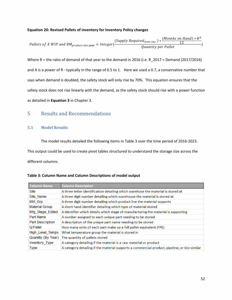
52
Equation 20: Revised Pallets of inventory for Inventory Policy changes
𝑃𝑎𝑙𝑙𝑒𝑡𝑠 𝑜𝑓 𝑋 𝑊𝐼𝑃 𝑎𝑛𝑑 𝑅𝑀𝑝𝑟𝑜𝑑𝑢𝑐𝑡 𝑠𝑖𝑡𝑒 𝒚𝒆𝒂𝒓 = 𝐼𝑛𝑡𝑒𝑔𝑒𝑟((𝑆𝑢𝑝𝑝𝑙𝑦 𝑅𝑒𝑞𝑢𝑖𝑟𝑒𝑑𝑖𝑡𝑒𝑚 𝑠𝑖𝑡𝑒 ) ∗
(𝑀𝑜𝑛𝑡ℎ𝑠 𝑜𝑛 𝐻𝑎𝑛𝑑) ∗ 𝑅𝐴
12𝑄𝑢𝑎𝑛𝑡𝑖𝑡𝑦 𝑝𝑒𝑟 𝑃𝑎𝑙𝑙𝑒𝑡
)
Where R = the ratio of demand of that year to the demand in 2016 (i.e. R_2017 = Demand (2017/2016)
and A is a power of R - typically in the range of 0.5 to 1. Here we used a 0.7, a conservative number that
says when demand is doubled, the safety stock will only rise by 70%. This equation ensures that the
safety stock does not rise linearly with the demand, as the safety stock should rise with a power function
as detailed in Equation 3 in Chapter 3.
5 Results and Recommendations
5.1 Model Results
The model results detailed the following items in Table 3 over the time period of 2016-2023.
This output could be used to create pivot tables structured to understand the storage size across the
different columns.
Table 3: Column Name and Column Descriptions of model output

53
The model accuracy was compared to the short term models results, and was found to be +-10%
for each of the matl_sub_groups from the years 2017 and 2018, which when aggregated, the overall
model was +-10% for each site. Moving forward, the model should be re-ran every time the LRP is
updated to determine the differences between the LRP.
The data was used to create multiple reports, most importantly the capacity utilization of each
warehouse by temperature requirements. This information for the baseline model is shown in Table 4.
This table shows a steady increase of warehouse utilization at most warehouses, and ABR and ASM
running out of capacity in the near time.
Table 4: Capacity Utilization of baseline model for each warehouse by temperature type
Once the overall warehouse capacity utilization was found for the next eight years, and each
scenario tested, a cost-benefit analysis was created. The utilization numbers were found for the
optimistic, baseline, and pessimistic cases of warehouse utilization, the pallet-years over capacity, and
the subsequent NPV to expense the 3PL storage to mitigate the over-utilization, were found to
determine the decisions to make additional capacity by adding warehouse space, or buy capacity from a
3PL. The results of this analysis are shown in Table 5 .
Table 5: Model Predictions of over-utilization associated expense based on demand scenarios
2-8C Utilization CRT Utilization
Site A B C D E F Site A B C D E F
2016 79% 115% 62% 9% 47% 19% 2016 37% 38% 48% 41% 13% 125%
2017 60% 166% 76% 80% 14% 46% 2017 66% 89% 42% 51% 46% 113%
2018 58% 198% 88% 46% 81% 279% 2018 59% 97% 13% 40% 60% 477%
2019 67% 191% 95% 27% 67% 164% 2019 58% 105% 14% 35% 70% 522%
2020 68% 196% 95% 18% 61% 196% 2020 62% 112% 9% 35% 67% 503%
2021 68% 200% 96% 19% 63% 193% 2021 64% 119% 7% 37% 67% 529%
2022 73% 202% 99% 19% 63% 200% 2022 67% 123% 8% 38% 68% 542%
2023 73% 201% 101% 18% 65% 179% 2023 68% 124% 7% 37% 68% 526%

54
Other scenarios identified in Chapter 4 assist to determine the best methods to mitigate over
utilization were calculated for the quantity of pallet-years over capacity over the eight year period, and a
NPV of the pallets to store at the 3PL’s for each warehouse. The results are displayed in Table 6. This
shows that, out of the scenarios identified, inventory policies discussed in Chapter 3 are the biggest
lever to reduce over-utilization and to reduce risks, followed by leveraging the existing network, and
continuous improvement opportunities at the warehouse sites.4 By using a scientifically calculated
inventory possibility, the over-utilization of the warehouses of the baseline demand could be reduced by
over 50%, while better utilization of the network could reduce over-utilization by 12%. Note that this is
not an either or option. All three policies could be simultaneously run to reduce overutilization.
Table 6: Model predictions of over-utilization associated expense of warehouse network
5.2 Warehouse Strategy Creation
Amgen’s Executive Vice President is quoted saying, “the supply chain strategy should be aligned
with the overall operations strategy”. Based on this, Amgen’s operations are transitioning to a modular,
variable based production strategy, away from asset heavy, large, fixed - production systems. So must
the warehouse strategy.
Given the results of Chapter 5.1, the analysis shows that the NPV of 3PL’s is lower than the expense of building additional capacity of warehouses for all scenarios as shown in
Table 5. The analysis also shows the best way to mitigate overutilization of warehouse capacity
would be to update the inventory policies. Amgen’s current practice is to use a flat MOH level for raw
materials = {Cycle Stock} + {Operations Safety Stock}. That is, raw materials operational safety stock
4 This is calculated on by the benefit of the scenario. Costs were not considered, which could be a significant
factor. As shown in Chapter 3, inventory policies could reduce risks, but must be considered thoughtfully.
55
inventory increases linearly with therapeutics demand. Using this logic in the model demonstrates that
our current practice inventory increases proportionally with volume, but according to Equation 20,
inventory should actually increase at a 0.8 power function of reorder frequency (which is a proxy for
volume). The Raw Materials & Devices team recognizes this mathematical function and recommends it
to the site supply chain teams, but the sites set their own (often proportional) levels. The opportunity of
implementing the Operational Safety Stock based on the aforementioned power function is a theoretical
$219M NPV (8%, FY 2017-2023 in lower working capital and a 3PL storage reduction of 6,000 pallet-year
space across the network.
The opportunity from changing fixed MFC policy for therapeutics WIP and finished product
Operational Safety Stock to one that varies at a 0.8 power function of volume opens up a large possible
opportunity in less working capital and a 3PL storage reduction of 14,000 pallet-year fewer space across
the network. This approach is made that much more powerful and reduces risk if Amgen increases nude
DP by reducing FDP and focus on improving lead times from DP to customers. The mathematical driver is
that risk pooling IDP across a larger market base will pool the variation utilizing the lessons in Chapter 3,
further increasing the opportunity to decrease Operational Safety Stock, (and possibly Strategic Safety
Stock). To affect this change, Amgen will have to become more nimble; quantitatively this means
reducing L (lead time) and decreasing R by increasing reorder frequency. There will, undoubtedly, be
many operational complexities, but the opportunity is large and worth exploring.
Amgen currently is using significant external warehouse space at Site B and Site E. This
overutilization will increase significantly next year. Site E is forecasted to start drawing more heavily on
external space next year (albeit, the space requirement based on the 5th pass 2016 LRP is less than
forecast from the 1st pass). The current therapeutics flow is Site B (or supplier) >> Site D >> 3PL >> Site
D. A better approach would be Site B (supplier) >> 3PL >> Site D. This would lower warehouse labor,
transportation costs, and risk through 25% less movements. In order to accomplish this, a project would
56
have to be started at each warehouse, and SAP would have to be updated to reflect the inventory at
3PL’s.
One of the tenants of lean manufacturing is a production system must be set. Due to Amgen’s
flexibility, the site supply chain managers have to be ready to produce any therapeutics when signaled
to. This necessitates the need to carry a larger inventory of raw materials, and due to not knowing the
next time therapeutics will be manufactured, a correspondingly high cycle and operational safety stock.
By setting the production cycle, and having an agreed start date for manufacturing, the site supply chain
teams will not have to store the inventory levels as high due to a lower variation of demand.
5.3 Supply Chain Communication
One of the best ways to prevent the dreaded bull whip effect as shown in Chapter 3 is proper
communication between roles. Some pathways could be improved to foster better communication and
results, such as the marketing team does not have an established communication pathway to each site’s
raw materials team. This leads to therapeutics being offered at discounts or different configurations
that quickly trigger unanticipated demand for raw materials, which drains safety stock due to the bull
whip effect. This problem is explored and solved in in Chapter 3. In addition to financial repercussions,
production could be more streamlined as production sometimes switches to product where the raw
materials are on hand. In addition, workforce stress could be reduced, as scrambles by supply chain and
manufacturing occurs to ensure production is not interrupted. The global supply chain managers also
could work with warehouse managers, and warehouse managers with each other, to work at pooling
raw materials and utilizing delay and push strategies for upstream and down- stream material moves.
By utilizing this strategy, the warehouses could free up ~ 5,000 pallet-years spaces and reduce 3PL costs
by $2.5M over 8 years.
57
5.4 Risk Mitigation Plan
The risk mitigation plans that detail which sites manufacturing capacity would take over if
another sites manufacturing capacity were brought down due to unforeseen risks were brilliantly
analyzed, but did not consider the warehouse capacity to store the raw materials needed to produce the
manufacturing. The analysis shows that most warehouses would not be able to support the risk
mitigation plans due to being overcapacity. To counteract this over-utilization and ensure the
warehouses will be able to support the added capacity, warehouse sites should create a risk mitigation
plan and develop options with a local 3PLs to be able to store necessary raw materials.
6 Future Work
This strategy only goes so far in recommending high level decision making, while there are many
projects that could be put into place that would further increase productivity and lower risk in the
warehouse network. They include the following areas:
Presently, the warehouses operate independently in identifying capacity overutilization,
continuous improvement activities to lower the overutilization, and the selection and handling
of inventory to a 3PL. Many activities must be standardized, including the following:
o Overflow storage for all non-critical inventories
o Overflow storage for all critical inventories
o True overflow with a shuttle between site and overflow
o SAP updates to factor inventory at 3PL sites
o Standards on make vs. buy and the different trigger in risk, cost, quality, etc.
Another scenario that should be studied would be an expansion of a warehouse that is known to
be over-utilized. Bids would need to be placed to add a specific amount of capacity, and then compared
with the model’s NPV analysis of the cost of 3PLs for each site. The costs for each warehouse
overutilization from the baseline models are shown in Table 7.

58
Table 7: Site NPV 3PL expense based on demand scenarios5
A wise man once said the following statement is always true, “You have roughly the right
amount of inventory, you just have too much of some stuff and not enough of the other stuff” (Sean
Willems, 2011). Much work could be started to look into the risk free methods of inventory
optimization. Moving from the Ad Hoc Frontiers to the Supply Chain Frontiers can lower safety stock
levels by 10-30%, while still ensuring “every patient, every time”. Simple projects such as risk pooling
and lead time reductions can make a drastic improvement, and free up warehouse capacity while saving
large amounts of working capital, and the subsequent holding cost. In order accomplish this, better
communication between the marketing units and site supply chain teams must be made, and lean
efforts to set the manufacturing schedule should be brought to minimize variation, and lead time
reductions accomplished. To get started on a scientifically calculated inventory policy, tracking the
errors of the LRP for each Stock Keeping Unit (SKU) should be accomplished to determine the demand
variation. This could be a moving monthly or quarterly deviation from the forecast. After finding this
value, it could be averaged out over time periods to determine the demand variation, which would be
an input for the safety stock calculations in Equation 3.
Once this is accomplished establish the base case by calculating the existing average inventory
level for each SKU. Next, scientifically calculate the expected inventory level using demand, lead-time,
and service information. Next, compare the two numbers and deep dive the differences. Present the
5 Site C’s has no known 3PL costs right now, and the over-utilization even for the optimistic demand scenario of
site C was minimal, so no calculation was performed.
:
CRT 2-8°C Total Costs CRT 2-8°C Total Costs CRT 2-8°C Total Costs
Site A $0 $0 $0 $0 $0 $0 $239,200 $2,106,053 $2,345,253
Site B $0 $683,009 $683,009 $992,106 $5,164,348 $6,156,454 $1,141,084 $8,711,773 $9,852,856
Site C N/A N/A N/A N/A N/A N/A N/A N/A N/A
Site D $0 $0 $0 $0 $0 $0 $0 $15,692,602 $15,692,602
Site E $0 $0 $0 $0 $0 $0 $101,162 $0 $101,162
Site F $6,296,814 $34,105 $6,330,919 $13,959,327 $363,222 $14,322,549 $18,358,796 $355,323 $18,714,119
Pessimistic Scenario Baseline Scenario Optimistic Scenario

59
detail but also offer general insights. As Sean Willems states, “convert data to information to knowledge
to wisdom”.
Strategic safety stock is an appropriate risk mitigation strategy for the risk of loss of
manufacturing capacity, but can be fine-tuned with Time to Survive (TTS) analysis. Amgen has
accomplished a good job at calculating Time-to-Recovery (TTR), the time it would take for a particular
node to be restored to full functionality after a disruption. An analysis of TTS, the maximum duration
that the supply chain can match supply with demand after a disruption, will provide the proper amount
of inventory to hold. Right now, Amgen utilizes strategic safety stock as the TTS, but do not utilize the
operational cycle and operational safety stock in this analysis. Amgen should consider the operational
cycle and safety stock as a TTS, and for the items that the TTS >> TTR, an inventory reduction project
could be started to mitigate the excess inventory.
7 Conclusion
In order to understand the impacts of growth on warehouse utilization, a relational database
inventory model was created and linked to the long range forecast of supply and demand. This
inventory model linked the Bill of Materials (BOMs) to the product forecast in order to understand the
quantity of raw materials required to meet the supply. The database also calculates the WIP and
finished product levels of Amgen’s products. This model considers inefficiencies in the warehouses, as
warehouse pallet spaces do not always store the maximum capacity of the material. This inventory
model calculated the capacity required for each warehouse over the forecasted ranges of FY 2016 to FY
2023. The findings of this model were used to create Amgen’s long term warehouse strategy. The
models forecast demonstrated a +- 10% accuracy to 2017 planning,
We developed a strategy that mimics Amgen’s operational strategy. Amgen’s Operational
strategy is to reduce fixed costs, and focus on flexibility with variable based costs. Based on this, we

60
found the best action was to work with 3rd party logistics providers (3PLs) to mitigate the capacity gaps
in a variable based manner. This option is preferred over investing in expanding capacity at warehouses
already in use for all three scenarios of optimistic, baseline, and pessimistic demand profiles.
The biggest lever to gain warehouse capacity is to improve inventory policies and the flow of
communication. Inventory policies whose aim is to reduce inventory can be viewed as a sensitive topic
at a company like Amgen. But, if done in a scientific manner, and moving from a Months on Hand
(MOH) approach to a scientifically calculated inventory, then moving to a multi-echelon inventory
optimization, inventory can be reduced while also reducing risk. The following are ways that can be
used to reduce inventory with little to no risk.
Track forecast error to understand variation of demand
Lead time reduction of raw materials and work in progress
Risk Pool Drug Product (DP) “nude” vials and decrease lead time from DP to customer
Re-order point frequency increases
Reduction of demand variability through:
o Better communication of demand forecasts between marketing, global supply chain,
and site supply chain teams.
o Reducing variability of manufacturing planning
Seek commonality of raw materials to lower safety stock levels
Multi-Echelon Inventory Optimization
Note that these are not either or choices, but can be combined projects to reduce risk and
becoming operationally more efficient. By accomplishing these activities, Amgen has a scope to reduce
working capital, reduce risk, and free up 20k pallet-year spaces over the same time period. This will also

61
lower the expense of 3PL costs and overall risks over the same time period. Considerable work will have
to be accomplished, but the benefits will outweigh the costs.
62
8 References Amgen Pipeline. (2016, October 17). Retrieved from Amgen: http://www.amgenpipeline.com/pipeline
Amgen Profitability Analysis. (2016, November 14). Retrieved from NASDAQ: Https://www.stock-
analysis-on.net/NASDAQ/Company/Angen-Inc/Ratios/Profitability
Amgen, I. (2016, February). 2015 Annual Report and 10-K. Thousand Oaks, California.
Choi, J. (2014). Raw Material Inventory Planning in a Serial System with Warehouse Capacity. Retrieved
from http://dspace.mit.edu/handle/1721.1/90775
David W. Thomas, J. B.-H. (2016, November 12). Clinical Development Success Rates 2006-2015.
Retrieved from Bio.org:
https://www.bio.org/sites/default/files/Clinical%20Development%20Success%20Rates%202006
-2015%20-%20BIO,%20Biomedtracker,%20Amplion%202016.pdf
Hau L. Lee, V. P. (1997, April 15). The Bullwhip Effect in Supply Chains. Retrieved from Sloan Review:
http://sloanreview.mit.edu/article/the-bullwhip-effect-in-supply-chains/
Information on Biosimilars. (2016). Retrieved from US Food and Drug Administration:
http://www.fda.gov/Drugs/DevelopmentApprovalProcess/HowDrugsareDevelopedandApprove
d/ApprovalApplications/TherapeuticBiologicApplications/Biosimilars/
Paul, S. M., Mytelka, D. S., Dunwiddie, C. T., Persinger, C. C., Munos, B. H., Lindborg, S. R., & Schacht, A.
L. (2010). How to improve R&D productivity: the pharmaceutical industry's grand challenge.
Nature.
REL . (2013). 2013 US Working Capital Survey. Retrieved from Relconsultancy.com:
http://www.relconsultancy.com/working-capital/2013-US-Working-Capital-Survey.pdf
Rosenfield, D. (2014). Innovation Economy. (R. Locke, & R. Wellhausen, Eds.) Cambridge: MIT Press.
Roza, S. (1998, May). Using Forecast Variability and Risk Pooling to Determine Optimal Safety Stock
Levels within a Supply Chain. Retrieved from LGO SDM Thesis Directory:
https://lgosdm.mit.edu/VCSS/servlet/LoadFile?VIEW=4&file=/Thesis/4069/roza98.pdf
Sean Willems, G. W. (2011). Inventory Optimization at Procter & Gamble: Achieving Real Benefits
through User Adoption of Inventory Tools. Interfaces, 66-78.
Simchi-Levi, D. (2010). Operations Rules. Cambridge: MIT Press.
Tversky, D. K. (1973, Jusly). On the Psychology of Prediction. Psychological Review.
Unknown. (2007). Benchmarking Study Project No. 63KV7601. Thousand Oaks: Amgen.
Unknown, A. (2016). Retrieved from The World Bank:
http://data.worldbank.org/indicator/IC.WRH.DURS?view=map&year=2016
63
Unknown, A. (2016, September 17). Amgen—A biotechnology success story: From drug development to
the mass market. Retrieved from MARSDD: https://www.marsdd.com/mars-library/amgen-a-
biotechnology-success-story-from-drug-development-to-the-mass-market/
Willems, S. (2015). Demystifying Inventory. Supply Chain Management Review, 24-30.
Yang, M. (2015). Optimization of Warehouse Operations and Transport Risk Mitigation for Disposable
Bio-reactor Bas to support launch of Amgen Singapore Manufacturing.

64
Appendix 1: Warehouse Capacity Model Details This is the user guide to update and maintain the Warehouse_Capacity_Model.accdb. This
database is used to approximate the warehouse capacity over the long term by linking the Long Range
Plan (LRP) and determining the inventory requirements based on BOMS and Safety Stocks. The
database also has other tools, such as the following:
Risk analysis, which determines the effects of a production sites mitigation efforts
Optimistic and Pessimistic scenarios for pipeline and commercial therapeutics demand
The following user guide will show you how to understand the model, how to update the model, and
how to get the most out of the model.
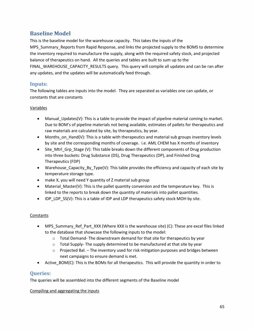
65
Baseline Model This is the baseline model for the warehouse capacity. This takes the inputs of the
MPS_Summary_Reports from Rapid Response, and links the projected supply to the BOMS to determine
the inventory required to manufacture the supply, along with the required safety stock, and projected
balance of therapeutics on hand. All the queries and tables are built to sum up to the
FINAL_WAREHOUSE_CAPACITY_RESULTS query. This query will compile all updates and can be ran after
any updates, and the updates will be automatically feed through.
Inputs: The following tables are inputs into the model. They are separated as variables one can update, or
constants that are constants
Variables
Manual_Updates(V): This is a table to provide the impact of pipeline material coming to market.
Due to BOM’s of pipeline materials not being available, estimates of pallets for therapeutics and
raw materials are calculated by site, by therapeutics, by year.
Months_on_Hand(V): This is a table with therapeutics and material sub groups inventory levels
by site and the corresponding months of coverage. i.e. AML CHEM has X months of inventory
Site_Mtrl_Grp_Stage (V): This table breaks down the different components of Drug production
into three buckets: Drug Substance (DS), Drug Therapeutics (DP), and Finished Drug
Therapeutics (FDP)
Warehouse_Capacity_By_Type(V): This table provides the efficiency and capacity of each site by
temperature storage type.
make X, you will need Y quantity of Z material sub group
Material_Master(V): This is the pallet quantity conversion and the temperature key. This is
linked to the reports to break down the quantity of materials into pallet quantities.
IDP_LDP_SS(V): This is a table of IDP and LDP therapeutics safety stock MOH by site.
Constants
MPS_Summary_Ref_Part_XXX (Where XXX is the warehouse site) (C): These are excel files linked
to the database that showcase the following inputs to the model:
o Total Demand- The downstream demand for that site for therapeutics by year
o Total Supply- The supply determined to be manufactured at that site by year
o Projected Bal. – The inventory used for risk mitigation purposes and bridges between
next campaigns to ensure demand is met.
Active_BOM(C): This is the BOMs for all therapeutics. This will provide the quantity in order to
Queries: The queries will be assembled into the different segments of the Baseline model
Compiling and aggregating the inputs
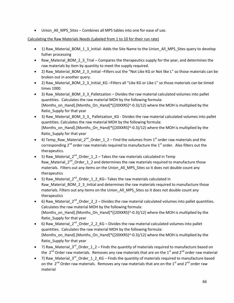
66
Union_All_MPS_Sites – Combines all MPS tables into one for ease of use.
Calculating the Raw Materials Needs (Labeled from 1 to 10 for their run rate)
1) Raw_Material_BOM_1_3_Initial- Adds the Site Name to the Union_All_MPS_Sites query to develop
futher processing
Raw_Material_BOM_2_3_Trial – Compares the therapeutics supply for the year, and determines the
raw materials by item by quantity to meet the supply required.
2) Raw_Material_BOM_2_3_Initial –Filters out the “Not Like KG or Not like L” so those materials can be
broken out in another query.
2) Raw_Material_BOM_2_3_Initial_KG –Filters all “Like KG or Like L” so those materials can be timed
times 1000.
3) Raw_Material_BOM_3_3_Palletzation – Divides the raw material calculated volumes into pallet
quantities. Calculates the raw material MOH by the following formula:
[Months_on_Hand].[Months_On_Hand]*([20XXRS]^-0.3)/12) where the MOH is multiplied by the
Ratio_Supply for that year
3) Raw_Material_BOM_3_3_ Palletzation_KG - Divides the raw material calculated volumes into pallet
quantities. Calculates the raw material MOH by the following formula:
[Months_on_Hand].[Months_On_Hand]*([20XXRS]^-0.3)/12) where the MOH is multiplied by the
Ratio_Supply for that year
4) Temp_Raw_Material_2nd_Order_1_2 – Find the volumes from 1st order raw materials and the
corresponding 2nd order raw materials required to manufacture the 1st order. Also filters out the
therapeutics.
5) Raw_Material_2nd_Order_1_2 – Takes the raw materials calculated in Temp
Raw_Material_2nd_Order_1_2 and determines the raw materials required to manufacture those
materials. Filters out any items on the Union_All_MPS_Sites so it does not double count any
therapeutics
5) Raw_Material_2nd_Order_1_2_KG– Takes the raw materials calculated in
Raw_Material_BOM_2_3_Initial and determines the raw materials required to manufacture those
materials. Filters out any items on the Union_All_MPS_Sites so it does not double count any
therapeutics
6) Raw_Material_2nd_Order_2_2 – Divides the raw material calculated volumes into pallet quantities.
Calculates the raw material MOH by the following formula:
[Months_on_Hand].[Months_On_Hand]*([20XXRS]^-0.3)/12) where the MOH is multiplied by the
Ratio_Supply for that year
6) Raw_Material_2nd_Order_2_2_KG – Divides the raw material calculated volumes into pallet
quantities. Calculates the raw material MOH by the following formula:
[Months_on_Hand].[Months_On_Hand]*([20XXRS]^-0.3)/12) where the MOH is multiplied by the
Ratio_Supply for that year
7) Raw_Material_3rd_Order_1_2 – Finds the quantity of materials required to manufacture based on
the 2nd Order raw materials. Removes any raw materials that are on the 1st and 2nd order raw material
7) Raw_Material_3rd_Order_1_2_KG – Finds the quantity of materials required to manufacture based
on the 2nd Order raw materials. Removes any raw materials that are on the 1st and 2nd order raw
material

67
8) Raw_Material_3rd_Order_2_3 – Filters out any raw materials that are on the 1st and 2nd order raw
materials queries
8) Raw_Material_3rd_Order_2_3_KG- Filters out any raw materials that are on the 1st and 2nd order raw
material queries.
9) Raw_Material_3rd_Order_3_3_Palletzation - Divides the raw material calculated volumes into pallet
quantities. Calculates the raw material MOH by the following formula:
[Months_on_Hand].[Months_On_Hand]*([20XXRS]^-0.3)/12) where the MOH is multiplied by the
Ratio_Supply for that year
9) Raw_Material_3rd_Order_3_3_Palletzation_KG - Divides the raw material calculated volumes into
pallet quantities. Calculates the raw material MOH by the following formula:
[Months_on_Hand].[Months_On_Hand]*([20XXRS]^-0.3)/12) where the MOH is multiplied by the
Ratio_Supply for that year
10) Total_Projected_Balance_RM – This is the summation of all the Raw Material queries into one
query.
Strategic Safety Stock
Total_Projected_Balance –Filters the Union_All_MPS_Sites query for Projected Balance, and divides the
projected balance quantity by the pallet quantity. This query provides the amount of finished
therapeutics and Work In Progress (WIP) that will be stored to ensure demand is met. Rapid Response
calculates this as the previous year’s projected balance –This year’s demand + This year’s supply
Safety_Stock_IDP_LDP_SS – Multiplies the Raw Material IDP and LDP by the IDP_LDP_SS for the MOH
safety stock for each site
Work in Progress
Total_Supply_WIP – Filters the Union_All_MPS_Sites query for Total Supply, and multiplies the total
supply quantity by Months_On_Hand to have MOH worth of Work in Progress at each site, divides by
the pallet quantity. This query provides the amount of finished therapeutics and Work In Progress
(WIP) that will be stored to ensure demand is met.
Outputs: FINAL_WAREHOUSE_CAPACITY_RESULTS - This is the final table for the baseline model. It adjusts the
total warehouse capacity needs found in Total_Projected_Balance_ALL by dividing each sites
warehouse needs by warehouse efficiencies.
Total_Projected_Balance_ALL – This is the overall sum of all pallets required to be stored. This
combines the Total_Projected_Balance and the Total_Supply_WIP and Total_Projected_Balance_RM
and the Safety_Stock_LDP into one
Risk Assessment This module of the database takes the baseline model results, and performs the playbook risk scenarios
for each site’s impacts on the other sites. This will showcase what the impacts of a site’s going down on
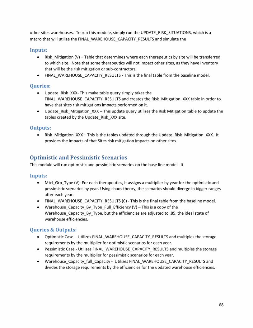
68
other sites warehouses. To run this module, simply run the UPDATE_RISK_SITUATIONS, which is a
macro that will utilize the FINAL_WAREHOUSE_CAPACITY_RESULTS and simulate the
Inputs: Risk_Mitigation (V) – Table that determines where each therapeutics by site will be transferred
to which site. Note that some therapeutics will not impact other sites, as they have inventory
that will be the risk mitigation or sub-contractors.
FINAL_WAREHOUSE_CAPACITY_RESULTS - This is the final table from the baseline model.
Queries:
Update_Risk_XXX- This make table query simply takes the
FINAL_WAREHOUSE_CAPACITY_RESULTS and creates the Risk_Mitigation_XXX table in order to
have that sites risk mitigations impacts performed on it.
Update_Risk_Mitigation_XXX – This update query utilizes the Risk Mitigation table to update the
tables created by the Update_Risk_XXX site.
Outputs: Risk_Mitigation_XXX – This is the tables updated through the Update_Risk_Mitigation_XXX. It
provides the impacts of that Sites risk mitigation impacts on other sites.
Optimistic and Pessimistic Scenarios This module will run optimistic and pessimistic scenarios on the base line model. It
Inputs: Mtrl_Grp_Type (V)- For each therapeutics, it assigns a multiplier by year for the optimistic and
pessimistic scenarios by year. Using chaos theory, the scenarios should diverge in bigger ranges
after each year.
FINAL_WAREHOUSE_CAPACITY_RESULTS (C) - This is the final table from the baseline model.
Warehouse_Capacity_By_Type_Full_Efficiency (V) – This is a copy of the
Warehouse_Capacity_By_Type, but the efficiencies are adjusted to .85, the ideal state of
warehouse efficiencies.
Queries & Outputs: Optimistic Case – Utilizes FINAL_WAREHOUSE_CAPACITY_RESULTS and multiples the storage
requirements by the multiplier for optimistic scenarios for each year.
Pessimistic Case - Utilizes FINAL_WAREHOUSE_CAPACITY_RESULTS and multiples the storage
requirements by the multiplier for pessimistic scenarios for each year.
Warehouse_Capacity_full_Capacity - Utilizes FINAL_WAREHOUSE_CAPACITY_RESULTS and
divides the storage requirements by the efficiencies for the updated warehouse efficiencies.
Top Related