


Languages
Pages
Legal


DETERMINATION OF POTENTIAL FAVORABLE ZONES
FOR PELAGIC FISH AGGREGATION (ANCHOVY) IN THE BLACK SEA
USING RS AND GIS
A THESIS SUBMITTED TO
THE GRADUATE SCHOOL OF NATURAL AND APPLIED SCIENCES
OF
MIDDLE EAST TECHNICAL UNIVERSITY
BY
NiLHAN ÇiFTÇi
IN PARTIAL FULFILLMENT OF THE REQUIREMENTS
FOR
THE DEGREE OF MASTER OF SCIENCE
IN
GEODETIC AND GEOGRAPHIC INFORMATION TECHNOLOGIES
MAY 2005

Approval of the Graduate School of Natural and Applied Sciences
__________________________ Prof. Dr. Canan Özgen
Director
I certify that this thesis satisfies all the requirements as a thesis for the degree
of Master of Science.
__________________________ Assist. Prof. Dr. Zuhal Akyürek
Head of Department
This is to certify that we have read this thesis and that in our opinion it is fully
adequate, in scope and quality, as a thesis for the degree of Master of Science.
__________________________ Assoc. Prof. Dr. Şükrü Beşiktepe Co - Supervisor
__________________________ Assist. Prof. Dr. Zuhal Akyürek Supervisor
Examining Committee Members
Prof. Dr. Vedat Topak (METU, GEOE ) ____________________
Assist. Prof. Dr. Zuhal Akyürek (METU, GGIT) ____________________
Assoc. Prof. Dr. Şükrü Beşiktepe (GAZİ, IMS) ____________________
Assist. Prof. Dr. Lütfi Süzen (METU, GEOE) ____________________
Assist. Prof. Dr. Hakan Mete Doğan (GOP, AGR) ____________________

iii
I hereby declare that all information in this document has been obtained and
presented in accordance with academic rules and ethical conduct. I also declare that,
as required by these rules and conduct, I have fully cited and referenced all material
and results that are not original to this work.
Name, Last name : Nilhan Çiftçi
Signature :

iv
ABSTRACT
DETERMINATION OF POTENTIAL FAVORABLE ZONES
FOR PELAGIC FISH AGGREGATION (ANCHOVY) IN THE BLACK SEA
USING RS AND GIS
Çiftçi, Nilhan
M. Sc., Department of Geodetic and Geographic Information Technologies
Supervisor: Assist. Prof. Dr. Zuhal Akyürek
Co-supervisor: Assoc. Prof. Dr. Şükrü Beşiktepe
May 2005, 107 Pages
Fishing is a significant source of food, and constitutes an important source of income
in Turkey. Due to the large extent required to analyse the distribution of fish stocks,
information derived from satellites play an important role in fisheries applications.
Chlorophyll concentration and sea surface temperature (SST) are the most significant
parameters which define the fish habitat. The accuracy of these parameters in the
Black Sea taken from two different satellites, namely Sea-viewing Wide Field-of-
views Sensor (SeaWIFS) and Moderate Resolution Imaging Spectroradiometer
(MODIS) are evaluated. Results indicate that both satellites give good estimates of
SST but the algorithms overestimate the chlorophyll concentration values. MODIS
products are used in the subsequent analyses due to their high correlation with in-situ
measurements relative to SeaWIFS products. The cause of the overestimation of
chlorophyll concentration is further examined and a general description of
environmental variability in Black Sea is done using MODIS products.
Anchovy, the most important commercial fish in Turkey, has been selected as the
target specie of the study. Level 3 weekly average MODIS chlorophyll and SST
products are processed using remote sensing (RS) and geographic information
systems (GIS) integration to estimate potential favorable zones for pelagic fish
aggregations.

v
Two different decision rules are employed to generate fish stock maps, simple
additive weigthing (SAW) and fuzzy additive weigthing (FSAW). The resultant
maps are used to visualize the general distribution of Anchovy in Turkish Seas from
May 2000 to May 2001. The resultant thematic fish stock maps generated by FSAW
analysis represents the uncertainity in the environment better than the ones generated
by SAW analysis.
Keywords: MODIS, SeaWIFS, Black Sea, Anchovy, Fuzzy Logic

vi
ÖZ
KARADENİZ’DE BULUNAN PELAJİK BALIK KÜMELERİNİN (HAMSİ)
TERCiH ETMESi MUHTEMEL POTANSiYEL ALANLARIN
UA VE CBS KULLANILARAK BELiRLENMESi
Çiftçi, Nilhan
Yüksek Lisans, Jeodezi ve Coğrafi Bilgi Teknolojileri Bölümü
Tez Yöneticisi: Y. Doç. Dr. Zuhal Akyürek
Ortak Tez Yöneticisi: Doç. Dr. Şükrü Beşiktepe
Mayıs 2005, 107 Sayfa
Balıkçılık vazgeçilmez bir besin kaynağı olmasının yanısıra aynı zamanda Türkiye
için önemli bir geçim kaynağıdır. Balık stoklarının dağılımının analizi için gerekli
olan geniş ölçek göz önüne alındığında; balıkçılık uygulamalarında uydu yolu ile
elde edilecek olan verilerin önemi daha iyi anlaşılmaktadır.
Balıkların yaşam alanlarının belirlenmesinde; klorofil yoğunluğu ve deniz suyu
yüzey sıcaklığı kullanılabilecek en belirgin değişkenlerdir. SeaWIFS ve MODIS
uydularından elde edilen görüntüler ile bu değişkenlerin Karadeniz’deki doğruluğu
değerlendirilmiştir. Her iki uydudan elde edilen veriler, deniz suyu yüzey sıcaklığı
açısından değerlendirildiğinde gerçek değerler ile oldukça yakın sonuçlar çıktığı
görülmüş fakat; uydulardan elde edilen verilerin değerlendirilmesinde kullanılan
algoritmalar klorofil yoğunluğunu, gerçek değerden daha yüksek saptamıştır.
Yerinde yapılan ölçümler ile uydulardan elde edilen veriler değerlendirildiğinde;
MODIS uydusundan elde edilen verilerin, SeaWIFS uydusundan elde edilen verilere
kıyasla yerinde yapılan ölçümler ile daha yüksek ilişki düzeyine sahip olduğu
saptandığından takip eden analizlerde MODIS uydusundan elde edilen veriler
kullanılmıştır.

vii
Klorofil yoğunluğunun gerçek değerinden daha yüksek saptanmasının nedenleri
anlatılmış ve Karadeniz’in çevresel değişiminin genel bir tanımı MODIS ürünleri
kullanılarak yapılmıştır.
Türkiye için en önemli ticari balık ürününün Hamsi olması sebebiyle; bu çalışmada
Hamsi hedef tür olarak seçilmiştir. MODIS uydusundan elde edilen Level 3 haftalık
ortalama klorofil yoğunluğu ve deniz suyu yüzey sıcaklığı ürünleri, Pelajik balık
kümelerinin tercih edeceği potansiyel alanların belirlenmesinde Uzaktan Algılama ve
Coğrafi Bilgi Sistemleri entegrasyonu ile değerlendirilmiştir. Balık stoğu
haritalarının üretilmesinde Basit Toplam Ağırlık (SAW) ve Bulanık Toplam Ağırlık
(FSAW) olmak üzere iki farklı karar verme yöntemi kullanılmıştır. Sonuçta ortaya
çıkarılan haritalarda, Mayıs 2000 ve Mayıs 2001 tarihleri arasında Karadeniz’de
Hamsi’nin genel dağılımı görülmektedir.
Anahtar Kelimeler: MODIS, SeaWIFS, Karadeniz, Hamsi, Bulanık Mantık

viii
to the memory of my grandfather
Ahmet Çiftçi

ix
ACKNOWLEDGEMENTS
I would like to express my sincerel thanks to my supervisor Assist. Prof. Dr. .Zuhal
Akyürek and my co-supervisor Assoc. Prof. Dr. Şükrü Beşiktepe for their continuous
support, their guidance, motivation and most of all their belief in me. I should admit
that it’s not a wise idea to study marine applications in Ankara.
I would like to thank my professors in Geological Engineering whom I have learned
a lot. Prof. Dr. Teoman Norman, knowing that he has publications in this area before
I was born, I admire his knowledge about marine studies. Prof. Dr. Vedat Toprak,
Prof. Dr. Vedat Doyuran, Assist. Prof. Dr. Lütfi Süzen, Dr. Arda Arcasoy and Dr.
Ertan Yeşilnacar. Your guidance means a lot to me. It was my pleasure to know you
all.
I would like to thank Assoc. Prof. Dr. Ahmet Cevdet Yalçıner from Coastal and
Harbour Engineering, for his assistance throughout my studies and his supportive
and positive approach.
I would like to thank Assoc. Prof. Dr. Doğan Yaşar from 9 Eylül Institute of Marine
Sciences and Technology, for his interest and support when I did not know anything
about marine studies in my first summer practice. The days I spent on R/V Piri Reis
was a great experience for me.
I would like to thank Assist. Prof. Dr. Hakan Mete Doğan for his concern and
appreciaiton.
I would like to thank to my friends in GGIT. Especially Ayhan Sağlam, Ali Özgün
Ok, Ebru Akpınar, Dilek Koç, Taner San and Kıvanç Ertugay for their support and
frienship.

x
I would like to thank to my friends in Set-üstü from METU Institute of Marine
Sciences, especially my close friend Adil Sözer, for his valuable advices.
I am thankful to my dear friends Ayşegül Domaç, Çağıl Kolat and Mine Ulusoy for
their valuable friendship throuhout my study in METU. I’m really glad to have
friends like you.
I thank Özgün Balkanay with all my heart, for being by my side in every decision I
make even if I’m right or wrong. His unlimited patience, encouragement and
motivation keeps me up, when things go wrong. Your smile lightens up my day
thank you for everything.
Growing by the sea side, I have learned to dive underwater before I learned to swim.
I would like to sincerely thank to my dear parents Nilüfer and Necati Çiftçi and my
lovely sister Ceylan, for making me who I am.
I would like to dedicate this work to the memory of my grandfather Ahmet Çiftçi. I
still remember how excited and happy I fell every time he told me stories about the
Turkish girl who became first in the swimming competition. Your memory will
remain in my heart forever, thank you...
It was my first year in university when I read a little article and decided to study
marine applications. Since then 8 years past, I can not say it’s an immediate success!
But now I believe the one can achieve anything, you only need to want it by heart
and go for it. I would like to express my thanks to all of you who were with me
during those years.
xi
TABLE OF CONTENTS
PLAGIARISM..................................................................................................................... iii
ABSTRACT........................................................................................................................ iv
ÖZ........................................................................................................................................ vi
DEDICATION.................................................................................................................... viii
ACKNOWLEDGEMENTS................................................................................................ ix
TABLE OF CONTENTS.................................................................................................... xi
LIST OF TABLES.............................................................................................................. xiii
LIST OF FIGURES............................................................................................................. xiv
LIST OF ABBREVIATIONS............................................................................................. xvii
CHAPTERS
1 INTRODUCTION.......................................................................................................... 1
1.1. Purpose and Objectives................................................................................................ 1
2 LITERATURE REVIEW.............................................................................................. 5
2.1. Description of Satellite Oceanography......................................................................... 5
2.1.1. Description of Marine Satellites................................................................... 5
2.1.2. Optical Properties of Black Sea.................................................................... 6
2.1.3. Overview of Validity of Algorithms ……………………………………... 8
2.2. RS and GIS Applicaitons in Fisheries.......................................................................... 10
2.2.1. Direct and Indirect Prediction Methods in Fisheries.................................... 10
2.2.2. Usage of Satellite Data in Fisheries Management........................................ 11
2.2.3. Integration of Multicriteria Decision Analysis and GIS............................... 13
2.2.4. Fisheries in Black Sea……………………………………………………... 14
3 METHODOLOGY AND MATERIALS...................................................................... 16
3.1. Methodology…………………………………………………………………………. 16
3.1.1. Definition of the Problem…………………………………………............. 17
3.1.2. Literature Survey………………………………………………….............. 17
3.2. Data Used……………………………………………………………………………. 17
3.2.1. In-situ Data…………………………………………………………........... 17
3.2.2. Satellite Data………………………………………………………............. 18
3.2.2.1. Ordering and Processing Satellite Data.……………………………18

xii
3.3. Evaluating Satellite Data…………………………………………………….............. 27
3.3.1. Evaluation of MODIS Products According to In-situ Measurements…….. 27
3.3.1.1. Chlorophyll Concentration Products……………………………............. 27
3.3.1.2. Sea Surface Temperature Products……………………………………… 30
3.3.2. Evaluation of SeaWIFS Products according to In-situ Measurements......... 32
3.3.2.1. Chlorophyll Concentration Products……………………………............. 32
3.3.2.2. Sea Surface Temperature Products……………………………………… 34
4 ANALYSES..................................................................................................................... 38
4.1. Description of Interannual Environmental Variability in Black Sea………………… 38
4.2. Determination of Potential Favorable Zones for Pelagic Fish Stocks in the
Black Sea…………………………………………………………………………………. 49
4.2.1. Determination of Potential Favorable Zones using SAW…………............ 49
4.2.1.1. Sea Surface Temperature Images.............................................................. 50
4.2.1.2. Chlorophyll Concentration Images............................................................ 56
4.2.1.3. Resultant Thematic Fish Stock Maps Generated by SAW........................ 61
4.2.2. Determination of Potential Favorable Zones using FSAW.......................... 66
4.2.2.1. Sea Surface Temperature Images.............................................................. 67
4.2.2.2. Chlorophyll Concentration Images............................................................ 72
4.2.2.3. Resultant Thematic Fish Stock Maps Generated by FSAW...................... 77
5 DISCUSSION.................................................................................................................. 82
5.1. Data............................................................................................................................... 82
5.2. Evaluation of the Satellite Imagery.............................................................................. 83
5.3. Description of Interannual Environmental Variablity in the Black Sea....................... 84
5.4. Determination of Potential Favorable Zones for Pelagic Fish Stocks......................... 84
6 CONCLUSION AND RECOMMENDATIONS……………………………………. 86
REFERENCES.................................................................................................................. 88
APPENDIX........................................................................................................................ 95

xiii
LIST OF TABLES
Table 2.1. Spectral and Spatial Differences Between Modis & Seawifs............................ 7
Table 3.1. Cruise Dates and the Coverage of In situ Measurements…………………….. 18
Table 3.2. Comparison in Evaluation Results……………………………………………. 36
Table 3.3. Dates of Satellite Imagery Used for the Evaluation………………………….. 37

xiv
LIST OF FIGURES
Figure 2.1. a) Main rivers flowing into Black Sea (After Barale et.al, 2002)
b) Multi-annual composites of water constituents concentration of the Black
Sea generated from Coastal Zone Color Scanner (CZCS)................................................. 9
Figure 3.1. Flowchart of the Methodology………………………………………………. 16
Figure 3.2. SEAWIFS Chlorophyll Concentration Parameter Imagery overlaid by
yellow triangles indicating the in-situ sample locations………………………………….. 19
Figure 3.3. Histogram Equalization of MODIS L2 Products............................................. 21
Figure 3.4. Reprojection of MODIS L2 Products.............................................................. 22
Figure 3.5. Rescaling MODIS L2 Products....................................................................... 23
Figure 3.6. Coding of MODIS L2 Products....................................................................... 24
Figure 3.7. Rescaling and Adding Pseudocolor to MODIS-Level 3 Products………….. 24
Figure 3.8. Histogram Equalization of MODIS L3 Products............................................. 25
Figure 3.9. Masking Extreme Values of MODIS L3 Products.......................................... 25
Figure 3.10. Masking Land Areas of MODIS L3 Products................................................ 26
Figure 3.11. Satellite Derived MODIS Chlorophyll_a Concentration Values Versus
In_situ Measurements.......................................................................................................... 28
Figure 3.12. Satellite Derived MODIS Chlorophyll_a Concentration Values Versus
In_situ Measurements in the First Cruise............................................................................ 28
Figure 3.13. Satellite Derived MODIS Chlorophyll_a Concentration Values Versus
In_situ Measurements in the Third Cruise.......................................................................... 29
Figure 3.14. Satellite Derived MODIS Chlorophyll_a Concentration Values Versus
In_situ Measurements in the Fifth Cruise........................................................................... 29
Figure 3.15. Satellite Derived MODIS SST Values Versus In-situ Measurements........... 31
Figure 3.16. Satellite Derived MODIS SST Values Versus In-situ Measurements
in the Black Sea................................................................................................................... 31
Figure 3.17. Satellite Derived MODIS SST Values Versus In-situ Measurements
in the Mediterranean............................................................................................................ 32
Figure 3.18. Satellite Derived SEAWIFS Chlorophyll_a Concentration Values Versus
In_situ Measurements.......................................................................................................... 33
Figure 3.19. Satellite Derived SEAWIFS Chlorophyll_a Concentration Values Versus
In_situ Measurements in the First Cruise............................................................................ 33

xv
Figure 3.20. Satellite Derived SEAWIFS Chlorophyll_a Concentration Values Versus
In_situ Measurements in the Third Cruise……………………………………………….. 34
Figure 3.21. Satellite Derived SEAWIFS SST Values Versus In_situ Measurements …. 35
Figure 3.22. Satellite Derived SEAWIFS SST Values Versus In_situ Measurements
in the Black Sea…………………………………………………………………………... 35
Figure 3.23. Satellite Derived SEAWIFS SST Values Versus In_situ Measurements
in the Mediterranean……………………………………………………………………… 36
Figure 4.1. a)Representation of the upper layer general circulation pattern of the Black
Sea. After Oğuz et al.( 1993). b) MODIS L3 chlorophyll concentration imagery
(24May-31May) c) MODIS L3 chlorophyll conc. imagery overlaid by
circulation pattern ………………………………………………………………………... 40
Figure 4.2. Thematic Map indicating the sub-regions in Blacksea
a- North Western Black Sea, b- Azov Sea, c- Pre-Bosphorous, d- Central Black Sea,
e- Battumi Gyre, f- South Eastern Black Sea…………………………………………….. 41
Figure 4.3. a) Annual Mean Chlorophyll-a Distribution of North Western Shelf
b)Annual Mean SST Distribution of North Western Shelf………………………………. 43
Figure 4.4. a) Annual Mean Chlorophyll-a Distribution of Azov Sea
b) Annual Mean SST Distribution of Azov Sea………………………………………….. 44
Figure 4.5. a) Annual Mean Chlorophyll-a Distribution of Pre_Bosphorous
b) Annual Mean SST Distribution of Pre_Bosphorous………………………………….. 45
Figure 4.6. a) Annual Mean Chlorophyll-a Distribution of Central Black Sea
b) Annual Mean SST Distribution of Central Black Sea………………………………… 46
Figure 4.7. a) Annual Mean Chlorophyll-a Distribution of Battumi Gyre
b) Annual Mean SST Distribution of Battumi Gyre…………………………………….. 47
Figure 4.8. a) Annual Mean Chlorophyll_a Distribution of South Eastern Blacksea
b) Annual Mean SST Distribution of South Eastern Blacksea…………………………… 48
Figure 4.9. Mean SST Distribution Throughout the Black Sea and the Temperature
Intervals............................................................................................................................... 50
Figure 4.10. Reclassified SST Distribution in Black Sea……………………………….. 52
Figure 4.11. Reclassified Chlorophyll Concentration Distribution in Black Sea………... 57
Figure 4.12. Resultant Thematic Fish Stock Maps Generated by SAW in Black Sea…... 62
Figure 4.13. Bell Shaped Membership Function Defining the SST Distribution
in Black Sea......................................................................................................................... 67
Figure 4.14. Reclassified SST Distribution in Black Sea with Bell Shaped Membership
Function…………………………………………………………………………………... 68
Figure 4.15. Trapezoidal Membership Function Defining the Chlorophyll Concentration

xvi
Distribution in Black Sea..................................................................................................... 72
Figure 4.16. Chlorophyll Concentration Distribution in Black Sea……………………... 73
Figure 4.17. Liner Membership Function for Generation of Thematic Fish Stock Maps.. 77
Figure 4.18. Distribution of Potential Favorable Zones for Pelagic Fish Stocks
in Black Sea Through FSAW…………………………………………………………….. 78
Figure A.1. Chlorophyll Concentration Distribution Gathered from MODIS
Chlorophyll-a Parameter in Black Sea…………………………………………………… 96
Figure A.2. SST Distribution Gathered from MODIS Sst4 Parameter in Black Sea……. 102

xvii
LIST OF ABBREVIATIONS
CDOM - Colored dissolved organic matter
CZCS - Coastal Zone Color Scanner
FSAW - Fuzzy additive weigthing SST- Sea surface temperature
GAC - Global Area Coverage
GIS - Geographic Information System
IMS - Institute of Marine Sciences
LAC - Local Area Coverage
LIDAR - Light Detection And Ranging
MCDA - Multi Criteria Decision Analyses
MHI - Marine Hydrophysical Institute
MODIS - Moderate Resolution Imaging Spectroradiometer
MSPHINX - MODIS Satellite Process Handling Images under Xwindow
OCS - Orbital Sciences Corporation
RS - Remote Sensing
RSDAS - Remote Sensing Data Analysis Service
SAW - Simple additive weigthing
SeaWIFS - Sea-viewing Wide Field-of-views Sensor
SEADAS - Seawifs Data Analysis System

1
CHAPTER 1
INTRODUCTION
1.1. Purpose and Objectives
Fishing is an important source of income in Turkey. The economic importance of
fishing brings the necessity of reaching marine resources with lower costs.
According to the State Institute of Statistics for year 2000, the total expenditure for
fishing activities is over 45 trillion Turkish Liras (DIE, 2002).
There are different types of expenditures, including liquid fuel and motor oil, special
wearing for fishing, toll, net and their repairing expenditures, food, water, electricity,
telephone and license expenditures, transportation and rent expenditures and some
other expenditures which are not quality of fixed capital. Liquid fuel and motor oil
expenditure is over 27 trillion Turkish Liras which holds the 60 % of all the
expenditures. To reduce the expenditure of fishing activity, it would be wiser to
reduce the fuel and motor oil expenditure. This is only possible by predicting the
potential locations of fish stocks to reduce the time spent for searching.
Satellite derived information plays an important role in fisheries applications.
Remote sensing techniques can be used directly for detection of fish stocks like
visual fish spotting from air crafts or these techniques can be used indirectly to
predict the potential favorable zones for fish aggregations by measuring the
parameters which affect the distribuiton of fishes (Butler et al., 1988).
2
The most frequently used parameter in studies that deal with relations between
environment, fish behaviour and abundance is sea temperature. Temperature has an
important influence over fish species at different stages of their life cycles and also
sea surface temperature (SST) is the most succesfully measured parameter among the
other satellite data measurements (Santos, 2000).
Phytoplankton biomass, which is the primary source of food within the sea is another
important parameter (Santos, 2000). Pyhtoplankton are microscopic marine
organisms which are responsible for most of the photosynthetic activity in the oceans
(Url 1). Phytoplankton, contain the pigment chlorophyll for photosynthesis. This
pigment reflects green and absorbs red and blue wavelengths of light. Different
algorithms to detect chlorophyll concentration are developed based on the optical
properties of phytoplankton. Although the algorithms may give erroneous results
due to the different absorption coefficients of species and available light (Morel and
Bricaud, 1981; Kirk, 1983), chlorophyll concentrations can be detected by satellites
and they are used as an indicator of available nutrient for marine organisms.
The aim of the study is to define the potential favorable locations for pelagic fish
stocks to decrease the fishing expenditures and consequently reach marine resources
with lower costs by the help of remote sensing and GIS integration.
Due to their direct effect on fishes, chlorophyll concentration and SST parameters are
utilized in the study. The accuracy of these parameters taken from two different
satellites, Sea-viewing Wide Field-of-views Sensor (SeaWIFS) and Moderate
Resolution Imaging Spectroradiometer (MODIS), are evaluated with respect to the
in-situ data. Both satellites give good estimates of SST but the algorithms
overestimate the chlorophyll concentration values in the Black Sea.
Ocean waters are divided into two classes according to their optical properties. In
case 1 waters, the concentration of phytoplankton and its associated chlorophyll and
covarying pigments define the optical properties. In this type of waters the
concentration of phytoplankton is usually low.

3
On the contrary, case 2 waters, are affected by many other substances, which do not
covary with chlorophyll. This type of waters may contain suspendend sediments,
colored dissolved organic matter (CDOM), gelbstoff, detritus and bacteria (Url 1;
Morel and Prieur, 1977 cited in Kendall et al., 1999).
Since the basin consist of case 2 type water, failure of the chlorophyll algorithms was
an expected result (Sancak et al., (2005), Yunev et al, 2002, Darecki and Stramski,
2004, Patissier et al., 2004).
MODIS algorithms give relatively better results than SeaWIFS algorithms in the
Black Sea. Thus MODIS products were processed to interpret the spatial and
temporal variations of SST and chlorophyll concentration in different sub-regions of
the area. General description of environmental variability in Black Sea and validity
of satellite driven information in marine applications have been stated in various
articles using Coastal Zone Color Scanner (Nezlin et al, 1999, Barale et al, 2002,
Kopelevich et al, 2002,) and SeaWIFS (Cokacar et al, 2001, Yunev et al., 2002,
Oguz et al., 2002,). However until now interpretation of Black Sea using MODIS
imagery has not been stated in the literature.
This general description also leads the determination of the areas that are favorable
for pelagic fish aggregations. The statistics show that the 77% of the total sea fish
catch by the year 2000 is catched in Black Sea and 82 % of this is Anchovy. In other
words, Anchovy holds the 63% of the total catch of sea fish in Turkey (DIE, 2002).
Being the most important commercial fish, Anchovy has been selected as the target
species in the study.
MODIS Level 3 (8 day composite) products are employed in the analyses. Two
different methods are used in generation of the potential favorable zones for pelagic
fish aggregations to visualize the general distribution of Anchovy in Turkish Seas
from May 2000 to May 2001.
The limitations of the avaliable in-situ data and the absence of information about fish
stocks and habitat preferences may yield some inconsistencies within the results.

4
However the overall accuracy of the SeaWIFS and MODIS algorithms and the
methodology of estimating potential favorable zones for pelagic fish aggregations are
explained in further chapters.
In Chapter 2 the literature review about the description of satellite oceanography and
RS-GIS applications in fisheries are stated, the metholodogy of the thesis and the
data used are explained in Chapter 3. The analyses are given in Chapter 4 which
defines the interannual environmental variability and the potential favorable zones
for pelagic fish stocks. Discussion, conclusion and recommendations are given in
Chapter 5 and Chapter 6 respectively.

5
CHAPTER 2
LITERATURE REVIEW
2.1. Description of Satellite Oceanography
2.1.1. Description of Marine Satellites
The color of water surface is determined by the color of pure ocean water and the
concentrations of different types of particles suspended in the upper water layer.
There are three major water color sensors to be used in oceanographic applications
(Url 2, 2005).
Coastal Zone Color Scanner (CZCS) on the Nimbus-7 satellite was developed by
NASA. It was designed to measure ocean color in terms of chlorophyll
concentrations and the distributions of particulate matter and dissolved substances. It
was operational from October 1978 until June 1986 and collected data on 6 identical
channels with 800 meter spatial resolution at nadir.
SeaWiFS on OrbView-2 satellite was launched on board an extended Pegasus launch
vehicle on August 1, 1997. OrbView-2 spacecraft and SeaWiFS radiometer were
developed by Orbimage Corporation in cooperation with NASA. It has 8 bands on
different wavelengths with spatial resolution of 1.1 km resolution and still
operational since 1997.
MODIS is an optical scanner aboard the Terra and Aqua satellites. Terra Satellite
launched on December 18th, 1999 and Aqua satellite on May 4, 2002. It has 36

6
channels with spatial resolution ranging from 250 meters to 1 kilometer. MODIS has
the ability to collect information on land, oceans, and atmosphere (Url 3). The
spectral and spatial resolutions of MODIS and SeaWIFS are given in Table 2.1.
SeaWiFS data can be downloaded free of charge for research work, but since the
SeaWiFS project is a partnership between NASA and a private company, Orbital
Sciences Corporation (OCS), researchers should register the SeaWiFs project and
obey specified restrictions. Once registered, they can obtain data older than 5 years
with no restrictions. MODIS Ocean data (Url 4) and CZCS data are free and have no
restrictions. Also further documentation on ocean color satellites and the softwares
are available on the NASA - Goddard Earth Sciences Distributed Active Archive
Center web page (Url 5, Url 6, Url 7).
2.1.2. Optical Properties of Black Sea
It’s hard to analyze case 2 waters relative to case1 waters due to their eutrophic
nature. However case 2 type waters are important in terms of their location, biologic
activity and their effect on algorithms. According to Acker (Url 1), case2 waters are
considerably more productive than case1 waters, which make these regions valuable
in terms of their contribution to global carbon cycle. Being more productive, case 2
waters are more reflective, and the atmospheric correction algorithms that is
dependent on the fact that “most ocean water is optically dark at certain wavelengths
becomes less reliable” (Url 1). Furtermore the location of case2 waters, which
covers usually the coastal areas, has a negative effect on the atmospheric correction
algorithms, due to the terrestrial contribution, haze of pollution and dust.
Morel and Bricaud (1981) and Kirk (1983) suggested that, the absorption coefficient
of phytoplankton, which the chlorophyll algorithms rely on, changes with species
type, size and nutrient and available light in the environment. As a result the effect
of case 2 waters on the algorithms is often misleading.

7
Table 2.1. Spectral and Spatial Differences Between Modis & Seawifs
MODIS SEAWIFS
Band Wavelength Region (µm)
Resolution
(m) Band Wavelength Region (nm)
Resolution
(km)
1 0.620-0.670 (red) 250 1 402-422 (blue) 1.13
2 0.841-0.876 (NIR) 250 2 433-453 (blue) 1.13
3 0.459-0.479 (blue) 500 3 480-500 (cyan) 1.13
4 0.545-0.565 (green) 500 4 500-520 (green) 1.13
5 1.230-1.250 (NIR) 500 5 545-565 (green) 1.13
6 1.628-1.652 (SWIR) 500 6 660-680 (red) 1.13
7 2.105-2.155 (SWIR) 500 7 745-785 (near-IR) 1.13
8 0.405-0.420 (blue) 1000 8 845-885 (near-IR) 1.13
9 0.438-0.448 (blue) 1000
10 0.483-0.493 (blue) 1000
11 0.526-0.536 (green) 1000
12 0.546-0.556 (green) 1000
13 0.662-0.672 (red) 1000
14 0.673-0.683 (red) 1000
15 0.743-0.753 (NIR) 1000
16 0.862-0.877 (NIR) 1000
17 0.890-0.920 (NIR) 1000
18 0.931-0.941 (NIR) 1000
19 0.915-0.965 (NIR) 1000
20 3.660-3.840 (TIR) 1000
21 3.929-3.989 (TIR) 1000
22 3.929-3.989 (TIR) 1000
23 4.020-4.080 (TIR) 1000
24 4.433-4.498 (TIR) 1000
25 4.482-4.549 (TIR) 1000
26 1.360-1.390 (NIR) 1000
27 6.535-6.895 (TIR) 1000
28 7.175-7.475 (TIR) 1000
29 8.400-8.700 (TIR) 1000
30 9.580-9.880 (TIR) 1000
31 10.780-11.280 (TIR) 1000
32 11.770-12.270 (TIR) 1000
33 13.185-13.485 (TIR) 1000
34 13.485-13.785 (TIR) 1000
35 13.785-14.085 (TIR) 1000
36 14.085-14.385 (TIR) 1000

8
The seasonal variability of the nutrient and light in the marine environment cause
changes in dominant species. Kendall et al. (Url 20) described that the remote
sensing reflectance model, which is used to develop the chlorophyll algorithm is site
and season specific. Since the properties of bio-optical constituents of water are not
stationary, they cannot be fixed and implemented for the entire case1 and case2
waters.
2.1.3. Overview of Validity of Algorithms
Barale et al. (2002), state that the CZCS, have been used to explore the historical
surface water optical conditions. Due to the limitations of the sensor it is not
possible to distinguish the suspended materials present in the water. Plumes
interacting with the marine environment, due to the major rivers the Danube, Dnestr
and Dnepr, and the Don flowing into the Sea of Azov, and the other minor inflows
can be seen in Figure 2.1.
Sancak et al., (2005), reflected that Mediterrenean and Black Sea can be described as
two extreme cases in terms of their bio-optical properties. Black Sea is dominated by
case 2 type waters and the failure of algorithms is expected. However the algorithms
also fail in detecting case 1 waters of Mediterranean, which can be due to their
specific optical properties.
Yunev et al., (2002) found that there is no statistically significant relationship
between Level 2 SeaWiFS imagery and in-situ chlorophyll-a within the open Black
Sea during 1997 to 2002. Utilizing daily Level 2 GAC SeaWiFS imagery opticians
from Marine Hydrophysical Institute (MHI), in Sevastopol, Ukraine have generated a
proper algorithm (MHI algorithm) to define chlorophyll-a concentration in Black
Sea. The generated algorithm has relatively better correlation with in-situ data than
SeaWIFS algorithm.

9
a)
b)
Figure 2.1. a) Main rivers flowing into Black Sea (After Barale et al., 2002)
b) Multi-annual composites of water constituents concentration of the Black Sea
generated from Coastal Zone Color Scanner (CZCS)
According to MODIS documentation there are three chlorophyll concentration
parameters, each derived using a different technique. These are; Chlorophyll
MODIS, Chlorophyll a SeaWIFS and Chlorophyll a semi-analytic. Each algorithm
provides the concentration of both case1 and case 2 waters. Chlorophyll MODIS is
derived using a 4 band algorithm. Chlorophyll a SeaWIFS (Chlor-a-2), is derived
from MODIS leaving radiances using the SeaWIFS algorithm. And Chlorophyll a

10
semi-analytic is derived from MODIS leaving radiances using multiple bands in an
analytical model (Url 6).
According to the evaluation of MODIS and SeaWIFS algorithms in Baltic Seas, both
of the algorithms overestimate the chlorophyll concentration. MODIS Chlor-a-2
parameter, which utilizes the SeaWIFS OC4 algorithm (Url 6) is found to give the
best results among other MODIS parameters. It is also stated that SeaWIFS
chlorophyll products have relatively higher accuracy than MODIS products. Yet
they still exhibit a significant overestimation of chlorophyll concentration in the
Baltic Sea. In order to create local algorithms, keeping the equations of the
algorithms the same, they have determined new coefficients from field
measurements. Darecki and Stramski (2004) reached the conclusion that, the
standard pigment algorithms will have inadequate accuracy even if region-specific
coefficients are utilized.
Patissier et. al., (2004) also state that SeaWiFS OC4v4 algorithm atmospherically
corrected for turbid waters with the Remote Sensing Data Analysis Service (RSDAS)
shows better results than MODIS algorithms in Northern European Seas. They
suggested that instead of using more complicated chlorophyll algorithms, improving
the atmospheric correction over optically complex waters results in more accurate
chlorophyll concentrations.
2.2. RS and GIS Applicaitons in Fisheries
2.2.1. Direct and Indirect Prediction Methods in Fisheries
Butler et al. (1998) stated that remote sensing techniques can be used directly or
indirectly in the prediction of fisheries resources. The direct methods comprise the
visual fish spotting from aircrafts, interpretation of aerial photographs, echo-
sounders, SONAR and Light Detection And Ranging (LIDAR) carried on aircraft.
Besides the indirect methods lie on the correlation of environmental parameters with
spatial and temporal distribution of fish aggregations.

11
Direct methods are limited by the range of aircraft and they are only reasonable when
the economic return of the catch compensates the expenditures of the aerial survey
(Butler et al., 1998). Thus the indirect methods are preferred. However indirect
methods also have some problems which are mainly caused by the accuracy of the
algorithms at different types of waters.
Valavanis et al., (2004) state that marine productivity hotspots are usually associated
with low sea surface temperature distribution due to the surfacing of deep nutrient
rich water masses and high chlorophyll concentration. They have created a GIS-
based model utilizing time series of SST distribution and chlorophyll concentration
gathered from satellite imagery. Combination of marine productivity hotspots and
seasonal catch of sardine, anchovy and pelagic squids revealing areas in the Eastern
Mediterranean are believed to indicate either as known overexploited fishing grounds
or new alternative unexploited fishing activity areas. Success of indirect
determination of fishes is dependent on previous knowledge of the habitat
preferences and behavior of the fish at different temperatures, information about the
oceanography of the area and catch rates occurring under specific conditions.
2.2.2. Usage of Satellite Data in Fisheries Management
Currents, circulation patterns, winds, sediment concentrations, water temperature,
and nutrients are the main parameters that define the fish habitat (Url 8). Among
these chlorophyll concentration and SST are the most significant indicators in the
fish habitat characterization (Santos, 2000).
The satellite measurements can only penetrate few meters into sea surface. Thus the
techniques used in defining the potential locations of fish stocks using satellite data
are valid for pelagic species only, which live near surface waters. Each pelagic
species has a certain tolerance of temperature and different annual migration pattern.
The characteristic habitats and behaviors of species allow the indirect determination
of potential favorable locations of these species using environmental parameters.
12
Furthermore to overcome the location and season specific effects of the environment,
forming a time series of the data would definitely increase the accuracy of the remote
sensing applications in fisheries management (Url 8).
Application of remote sensing to fisheries is widely utilized in various countries, for
albacore tuna fishery in North Pacific, shrimp fishery in Gulf of Mexico, sword
fishery in Portugal, and for monitoring the fishing zones in Japan, China, Taiwan,
India and Peru (Url 9).
NOAA's CoastWatch Program makes images and data available at the NOAA
CoastWatch web site in near real-time from various sensors and satellites. Each
type of image has many uses and temperature images indicating sea surface
temperature are used to locate fishing spots (Url 10).
Furthermore there are commercial companies providing information for fisheries
applications such as ORBIMAGE’s SeaStar Fisheries Information Service. SeaStar
Service claims that since 1997 it has significantly improve the efficiency of the fish
finding process based on plankton information obtained from SeaWIFS imagery of
OrbView-2 satellite, combined with other environmental data. SeaStar Service is
used by tuna and sardine purse seiners, pelagic longline and trolling vessels, and
midwater trawling vessels throughout the world. Enabling to find favorable fishing
locations, the service proposes to reduce the fuel costs in the fishing process (Url 11).
According to Food and Agriculture Organization of the United Nations (Url 12),
integration of satellite remote sensing and GIS, is increasingly used in marine and
inland fisheries projects. Especially among poor communities in coastal areas fish is
an important source of food. Nevertheless, due to the open access conditions in
fisheries, overexploitation threatens marine and inland stocks. “Effective
conservation and sustainable management of both marine and inland fisheries are
needed at national and international levels so that living aquatic resources can
continue to meet global nutritional needs” (Url 12).

13
2.2.3. Integration of Multicriteria Decision Analysis and GIS
GIS, is a computer-based system that enables acquisition, storage, retrieval,
modeling, manipulation and analysis of geographically related data (Aronoff, 1993).
According to Malczewski (1999), geographical data, information and decision
making are three concepts that are interrelated. Geographical data constitutes the
raw material and processed to gather information by decision making. Multi criteria
decision making (MCDM) or in other words, multi criteria decision analyses
(MCDA) evaluate a set of alternatives according to conflicting or unequal criteria.
MCDA problems mainly have 3 types of decision variables, deterministic,
probabilistic and fuzzy. Deterministic decisions assume that the required data and
information are known with certainity and between every decision and the
corresponding consequence there is a certain deterministing relation. The
probabilistic decisions deal with the situations which include uncertainty about the
state of the environment and about the relationship between the decision and its
consequences. Probabilistic analysis treats uncertainty as randomness and
likelihood, whereas fuzzy decision analysis deals with the uncertainty due to
imprecise information (Malczewski, 1999).
According to Zadeh (1998), "Fuzzy logic is the logic underlying approximate, rather
than exact, modes of reasoning. In fuzzy logic everything, including truth, is a
matter of degree." In other words, fuzzy logic is related with the formal principles of
approximate reasoning when the precise reasoning restricts the study.
Integration of RS and GIS is employed in the definition of potential favorable zones
for pelagic fish stocks. Since the conventional GIS applications utilize classical set
theory, they are inadequate to state the natural variability in the environment (Wang,
1996).
Fuzzy classification defines the classes as linguistic terms. The linguistic term is
used to express concepts and knowledge in human communication, whereas the

14
corresponding numerical data (membership function) is used for processing (Yen and
Langari, 1999).
Use of fuzzy set theory within GIS applications provides an approximate description
of the real world which is full of uncertainities. Membership functions and their
associated linguistic terms incorporate expert experiences in the form of vague
definitions to cell-based GIS analysis and make fuzzy set theory superior to the
classical set theory (Yanar and Akyürek, 2005).
2.2.4. Fisheries in Black Sea
According to State Institute of Statistics, Anchovy holds the 63% of the total catch of
sea fish in Turkey (DIE, 2002). Being the most important commercial pelagic fish in
Turkish Seas, Anchovy has been selected as the target specie of the study.
In Black Sea two subspecies of Anchovy are present, Engraulis encrasiholus
ponticus (the Black Sea Anchovy) and Engraulis encrasiholus maeoticus (the
Azovian Anchovy) (Salestenenko, 1955/56 cited in Bingel et al., 1995). The
Azovian Anchovy lives in the sea of Azov but overwinters in the warm waters of
Caucasus and Crimea (Sorokin, 2002), it is therefore fished only by Russia (Ivanov
and Beverton, 1985).
The Black Sea Anchovy exist in the Black Sea through out their annual life cycle,
but overwinter in the warmest parts of the Black Sea, off the Anatolian and Crimean
coasts. Anchovy start seasonal migrations to their wintering places, in the late
autumn, and return to their feeding and spawning grounds in spring (Ivanov and
Beverton, 1985).
Anchovy leave the wintering places on the Turkish coast and migrate to the north for
feeding and spawning in April. They remain dispersed over the whole Black Sea
especially in the northern part, from the middle of April until October. Southward
migration for wintering starts in November but it’s also affected from climatological

15
regime. The migration speed is 10-20 nautical miles per day. Through out the
migration anchovy may trace the topography of the coast or directly cross the sea
(Ivanov and Beverton, 1985). Anchovy start to move to wintering places when water
temperature is 15-17 °C following the slope egdes at 50-200 m depth (Chashin and
Alexeev, 1990 cited in Sorokin, 2002). They arrive to their wintering regions where
they form large schools over steep shelf area along Caucasian and Anatolian coasts,
when water temperature is 11-14 °C (Sorokin, 2002).
Life span of Anchovy changes between 2 to 3 years. They become mature after the
first winter and spawning continues from the end of May until September at water
temperatures 17-18 °C (Owen, 1979 cited in Ivanov and Beverton, 1985). To be able
to interpret the effecs of changing of environment on Anchovy, egg and larvae stages
should be observed carefully. Eggs develop into larvae within 24 hours, but highly
affected from the temperature. High mortality rates may be observed in May due to
the contact with cold water. The best period for spawning is from the end of june to
the beginning of July (Slastenenko, 1955/56 cited in Bingel, et al., 1995). Athough
the main spawning area of the Black Sea Anchovy is said to be the northern shelf
region (Ivanov and Beverton, 1985) studies showed that a significant amount of
Anchovy eggs are found within the Turkish Exclusive Economic Zone (Bingel, et al.,
1995; Kideys et al, 1999).

16
CHAPTER 3
METHODOLOGY AND MATERIALS
3.1. Methodology
The methodology of the thesis is described in this chapter and the main steps of the
study are given in the flowchart diagram in Figure 3.1.
Figure 3.1. Flowchart of the Methodology
Literature Survey
Data Preperation
Satellite Data In-situ measurements
MODIS Image
Processing
SEAWIFS Image
Processing
Evaluation of Satellite Data
Defining Fish Species
Definition of the Problem
Selection of Favorable Satellite Data and Algorithms
DATA
Description of Interannual
Environmental Variability
Potential Favorable Zones for Pelagic Fish Stocks Resultant Maps
GIS Analyses
EVALUATION
ANALYSES

17
3.1.1. Definition of the Problem
The aim of the study is to reach marine resources with lower costs. RS and GIS are
used in the study to define the potential favorable locations of pelagic fish species.
The problem is defined as the high cost of liquid fuel and motor oil consumption
while seeking for fish aggregations and consequently high expenditures for fishing
activity.
3.1.2. Literature Survey
The literature is examined and defining potential favorable zones for fish stocks
using satellite imagery is found to be the proper solution for the specified problem.
The studied literature is already explained in Chapter 2.
3.2. Data Used
The data used in the study are satellite images and in-situ water samples of SST and
chlorophyll concentration. Integration of Satellite information and fisheries require
previous knowledge of habitat preferences of the fish, behavior of a given species at
different temperatures, and catch rates occurring under those conditions (Earth
Science Enterprise). The habitat preferences of the Anchovy were gathered from the
literature but fish catch data for this specie was not available.
3.2.1. In-situ Data
The in-situ chlorophyll concentration and SST data were taken from METU Institute
of Marine Sciences (IMS) archive, which were previously collected onboard R/V
Bilim. Chlorophyll-a concentration was measured by the fluorometric method.
Water samples were collected from the euphotic zone. 1 to 2 litres of seawater was
filtered through filters and processed in METU-IMS. In-situ data was employed for
the evaluation of satellite imagery algorithms for our seas. Thus a combination of in-
situ datasets and imagery captured on the same date (or within 1 day interval when
there is insufficient data) were collected. Due to the absence of satellite imagery and
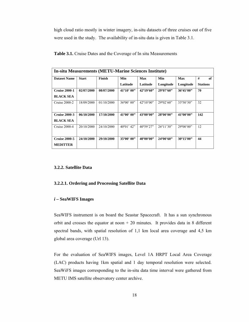
18
high cloud ratio mostly in winter imagery, in-situ datasets of three cruises out of five
were used in the study. The availability of in-situ data is given in Table 3.1.
Table 3.1. Cruise Dates and the Coverage of In situ Measurements
3.2.2. Satellite Data
3.2.2.1. Ordering and Processing Satellite Data
i – SeaWIFS Images
SeaWIFS instrument is on board the Seastar Spacecraft. It has a sun synchronous
orbit and crosses the equator at noon + 20 minutes. It provides data in 8 different
spectral bands, with spatial resolution of 1,1 km local area coverage and 4,5 km
global area coverage (Url 13).
For the evaluation of SeaWIFS images, Level 1A HRPT Local Area Coverage
(LAC) products having 1km spatial and 1 day temporal resolution were selected.
SeaWiFS images corresponding to the in-situ data time interval were gathered from
METU IMS satellite observatory center archive.
In-situ Measurements (METU-Marine Sciences Institute) Dataset Name Start Finish Min
Latitude
Max
Latitude
Min
Longitude
Max
Longitude
# of
Stations
Cruise 2000-1
BLACK SEA
02/07/2000 08/07/2000 41º10’ 00” 42º19’60” 29º07’60” 36º45’00” 70
Cruise 2000-2
18/09/2000 01/10/2000 36º00’ 00” 42º10’00” 29º02’60” 33º50’50” 32
Cruise 2000-3
BLACK SEA
06/10/2000 17/10/2000 41º00’ 00” 43º00’00” 28º00’00” 41º00’00” 142
Cruise 2000-4
20/10/2000 24/10/2000 40º01’ 42” 40º59’27” 26º11’30” 29º00’00” 12
Cruise 2000-5
MEDITTER
24/10/2000 29/10/2000 35º00’ 00” 40º00’00” 24º00’60” 30º15’00” 44

19
HRPT file consist of the scans received by the ground station while the satellite is
above the station's receiving horizon. Processing Level l A HRPT LAC to Level 2
requires additional steps. SeaWiFS Data Analysis System (SeaDAS), working in the
UNIX environment, is used for processing Level 1A data to Level 2. Ancillary
meteorological data and ozone data is used for atmospheric correction. Using the
default settings of the SeaDAS software the geophysical products are produced. In
Figure 3.2. SeaWIFS processed chlorophyll concentration parameter is given (Url
14).
Generated SST and chlorophyll concentration images were analyzed using SeaDAS
software. The pixel value in the SeaWiFS image that corresponds to the in situ
value was taken as the nearest pixel to the exact location. Assuming that the mean
value would give better results than the centre pixel value, a 3x3 pixel area centred
on that nearest pixel was selected to read the value of SeaWiFS derived parameters.
Then the mean value of 9 pixels was calculated and assigned as the final value to be
used in the accuracy evaluation analyses.
Figure 3.2. SEAWIFS Chlorophyll Concentration Parameter Imagery Overlaid by
Yellow Triangles Indicating the In-situ Sample Locations.

20
ii- MODIS Images
MODIS is an Earth-observing instrument on board the Terra (EOS AM) and Aqua
(EOS PM) satellites. Terra passes from north to south across the equator in the
morning, while Aqua passes south to north over the equator in the afternoon.
MODIS Terra and Aqua view the entire Earth's surface every 1 to 2 days and provide
data in 36 spectral bands with spatial resolutions of 250m (bands 1-2), 500m (bands
3-7) and 1000m (bands 8-36) (Url 15).
MODIS Images can be downloaded from NASA - Goddard Earth Sciences
Distributed Active Archive Center (DAAC) free of charge (Url 16).
MODIS Terra product archive contains imagery from February 2000 to present,
while MODIS Aqua product archive starts from November 2002. Therefore MODIS
Terra products are used in the analyses.
Over 100 categories of MODIS Ocean data types can be obtained from the Goddard
DAAC. MODIS ocean data types consist of ocean color, sea surface temperature,
and ocean primary production. Ocean color and sea surface temperature products are
available at processing Level 2 and Level 3 and ocean primary production data are
available as Level 4 data (Url 17).
Two different levels of MODIS-Terra Ocean Products were utilized throughout the
study. For evaluation purposes Level 2 products with 1km spatial, 1 day temporal
resolution and for the fisheries applications Level 3 products with 4.89 km spatial
and 8 day temporal resolution were utilized. Having higher spatial resolution than
Level 3 products, Level 2 products are preferred for evaluation analyses to increase
the level of detail that can be extracted from the imagery. Since in the analyses the
correlation of the pixel values and the in-situ data is evaluated, it would be more
relevant to match the in-situ data with higher resolution imagery. Furthermore Level
2 products have 1 km spatial resolution, identical to SeaWIFS imagery, which is
preferred for the comparison of the accuracy results. One disadvantage of Level 2
imagery is that, having higher resolution, they are bigger in size. In the description
21
of inter annual environmental variability and fish stock analyses, a time series of
satellite imagery is occupied. MODIS imagery comprising three chlorophyll
concentration parameters and two SST parameters for the whole year were
downloaded via ftp. To avoid the heavy data load in downloading, making analyses
and also in data storage, Level 3 products, which also have enough resolution for the
description of inter annual environmental variability and fish stock analyses were
utilized in further analyses. Level 3 images have a global coverage so before the
analyses; each Level 3 image is cropped according to the study area. On the contrary
Level 2 images are available as subsets.
All the products were processed using MSPHINX (MODIS Satellite Process
Handling Images uNder Xwindow) software. This is free UNIX software, designed
by Laboratoire d'Optique Atmospherique, a French planetary research institution. It
is available via web (Url 18).
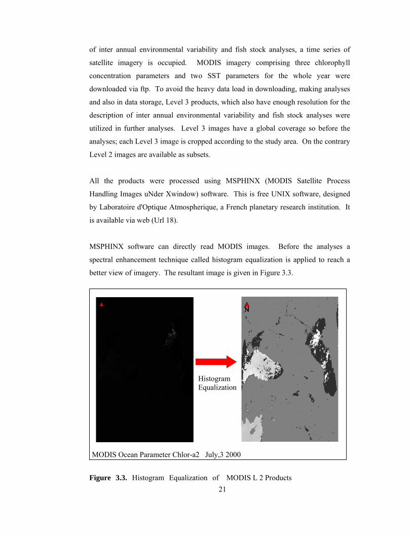
MSPHINX software can directly read MODIS images. Before the analyses a
spectral enhancement technique called histogram equalization is applied to reach a
better view of imagery. The resultant image is given in Figure 3.3.
Figure 3.3. Histogram Equalization of MODIS L 2 Products
Histogram Equalization
MODIS Ocean Parameter Chlor-a2 July,3 2000

22
Level 2 images need more processing due to the distortion in this level of MODIS
imagery, called the panoramic bowtie effect. As it is seen in Figure 3.3 the image is
distorted near the edges. The reason of the distortion is that MODIS scans 10 lines at
a single pass, whereas SeaWIFS scans 1 line at a time. As the distance between the
sensor and the pixel location increases, the pixel size increases accordingly. Thus the
pixels near the edge of an image are bigger than the ones in the middle. On the scan
line the pixel sizes are identical to each other, whereas as the scan angle decreases
the pixels might be 6 times wider and 4 timer longer at the edges (Url 19).
MSPHINX reprojects Level 2 products to a standard projection and remove the bow
tie artifacts using geolocation products of MODIS imagery. The reprojected MODIS
imagery can be seen in Figure 3.4.
Figure 3.4. Reprojection of MODIS L2 Products
MODIS products provide many paramaters for oceanographic studies. In Figure 3.4
the parameter indicating chlorophyll-a pigment concentration is given. This product
gives the chlorophyll-a pigment concentration in terms of mg/m3. In the legend, it is
seen that the pixel values start from 2000 and rises up to 65535. This indicates that
MODIS Ocean Parameter Chlor-a2 July,3 2000

23
the Level 2 images also need to be rescaled. Rescaling process is also done in
MSPHINX and the chlorophyll concentration distribuiton is gathered in terms of
mg/m3. Figure 3.5 represents the rescaled imagery.
Figure 3.5. Rescaling MODIS L2 Products
The processed image is displayed in color as in Figure 3.6 for better visual
interpretation and used in the evaluation analyses.
Assuming that the mean value would give better results than the centre pixel value,
again a 3x3 pixel area centred on that nearest pixel was selected to read the value of
MODIS derived parameters. The mean value of 9 pixels was calculated and assigned
as the final value to be used in the analyses. The correlation of those values and the
in-situ data is examined to asses the accuracy of the satellite algorithms.
Processing of Level 3 images are identical to Level 2 image processing. But Level 3
images are easier to process since they are not distorted. Adding pseudocolor and
rescaling of imagery is done by MSPHINX and the resultant imagery is given in
Figure 3.7.
MODIS Ocean Parameter Chlor-a2

24
Figure 3.6. Coding of MODIS L 2 Products
Figure 3.7. Rescaling and Adding Pseudocolor to MODIS L3 Products
Spectral enhancement techniques are applied to improve the interpretability of the
chlorophyll concentration images as seen in Figure 3.8.
MODIS Ocean Parameter Chlor-a2 Apr,14 2000
MODIS Ocean Parameter Chlor-a2 July,3 2000

25
Figure 3.8. Histogram Equalization of MODIS L 3 Products
Figure 3.9. Masking Extreme Values of MODIS L 3 Products
MODIS Ocean Parameter Chlor-a2 Apr.14, 2000
MODIS Ocean Parameter Chlor-a2 Apr,14 2000

26
Even if the results are overestimated according to the literature (Yunev, 2002) the
concentration values over 60mg/m3 is assumed to be erroneous and neglected during
the processes, given in Figure 3.9.
Finally the land areas are masked to overcome the confusion in the further analyses
and for a better visual appearance. The resultant imagery is given in Figure 3.10.
Figure 3.10. Masking Land Areas of MODIS L3 Products
Level 3 images are used in two different kinds of analyses. First one is to interprete
the interannual environmental variability and the second is the determination of
potential favorable locations for pelagic fish stocks. The analyses steps are explained
in the fourth chapter.
MODIS Ocean Parameter Chlor-a2 Apr,14 2000
27
3.3. Evaluating Satellite Data
Although the characteristics of marine environment differ from region to region, like
the Black Sea and the Mediterranean, the algorithms used in the satellites are global.
Accuracy of the satellite driven data is directly related with the satellite algorithms,
but unfortunately regional algorithms for the Turkish Seas have not been developed
yet. Since we lack the information that confirms the validity of the satellite data in
our seas, before the analyses, SeaWIFS and MODIS chlorophyll and SST products
are evaluated according to in-situ measurements taken from the seas around Turkey.
The evaluation results are examined in this chapter.
3.3.1. Evaluation of MODIS Products According to In-situ Measurements
3.3.1.1. Chlorophyll Concentration Products
MODIS chlorophyll concentration parameters are evaluated. Chlorophyll-a
(SeaWIFS), in other words Parameter 26, which has the highest correlation with in-
situ data is used in the analyses. This parameter utilize the SeaWIFS "OC4"
algorithm using MODIS water-leaving radiances and valid for both case 1 and case 2
waters (Url 15). The algorithm needs input of the water-leaving radiance bands
centered at 412, 443, 488, and 551 µm. (Url 20).
Figure 3.11. represents the correlation of all the in-situ data taken in different cruises
and the satellite derived values. Each cruise has taken place either in different seas
or in different times as it can be in seen in Table 3.1. There are three subgroups
within the graphic. So the data is divided into three groups, representing different
cruises.
Cruise 1 indicates the measurements taken from Black Sea in summer. As it is seen
in Figure 3.12 although the correlation of in-situ chlorophyll-a data with the satellite
derived ones are high, the equation shows that satellite derived concentration values
are seven times higher than in-situ results.

28
Cruise 1/3/5
y = 2.7311xR2 = -0.4612
00.5
11.5
22.5
3
0 0.5 1 1.5 2 2.5 3
In-situ chlor(tot)
MO
DIS
chl
-a-2
Figure 3.11. Satellite Derived MODIS Chlorophyll_a Concentration Values Versus
In_situ Measurements
Cruise 1
y = 7.068xR2 = 0.7365
00.5
11.5
22.5
3
0 0.5 1 1.5 2 2.5 3
In-situ chlor(tot)
MO
DIS
chl
-a-2
Figure 3.12. Satellite Derived MODIS Chlorophyll_a Concentration Values Versus
In_situ Measurements in the First Cruise
MODIS algorithm highly overestimates the chlorophyll concentration values. Black
Sea is Case 2 type of water, which is mostly problematic for the algorithms and this
might also indicate that certain species can cause failure of the algorithms.
According to the MODIS Algorithm Theoretical Basis Document, the remote sensing

29
reflectance model used to develop the chlorophyll algorithms has a few parameters
that cannot be fixed and applied to the entire globe; as a result, they are site and
season specific. This is due to the variability of many bio-optical constituents. For
example, absorption at 440 nm per unit chlorophyll a by phytoplankton can change
with species and with nutrient and lighting conditions by as much as a factor of 5
(Morel and Bricaud, 1981; Kirk, 1983; Carder et al., 1991; Morel et al., 1993).
Cruise 3
y = 1.9017xR2 = 0.5226
0
0.5
1
1.5
0 0.5 1 1.5
In-situ chlor(tot)
MO
DIS
chl
-a-2
Figure 3.13. Satellite Derived MODIS Chlorophyll_a Concentration Values Versus
In_situ Measurements in the Third Cruise
Cruise 5
y = 2.6545xR2 = 0.9369
0
0.5
1
1.5
0 0.5 1 1.5
In-situ chlor(tot)
MO
DIS
chl
-a-2
Figure 3.14. Satellite Derived MODIS Chlorophyll_a Concentration Values Versus
In_situ Measurements in the Fifth Cruise

30
The results of Cruise 3, which was taken place in Black Sea like Cruise 1 but in
different season, give only two times higher results as indicated in Figure 3.13. This
might lead to the conclusion that the increase of certain type of species that cause the
failure of the algorithms due to season changes. Moreover, cruise 3 represents
autumn, cruise 1 represents summer period. Since algorithms are affected by solar
contamination, the difference between the satellite measurements and the in-situ
values might occur due to the different illumination conditions instead of different
species.
Cruise 5 represents Mediterranean Sea. Due to the fact that the Mediterranean Sea is
case 1 water, the correlation within the data is higher. But as it is represented in
Figure 3.14 the number of in-situ data is insufficient. Thus, although high
correlation value is expected, the result is not reliable.
3.3.1.2. Sea Surface Temperature Products
There are two MODIS SST algorithms namely sst and sst4. According to the MODIS
documentation sst4 is composed of three bands near 4µm which are mid-infrared
bands. SST algorithm have two far-infrared bands which are between 10 and 12µm.
It is also stated that the atmospheric window covering mid-infrared bands is more
transparent than the one covering far-infrared bands, which provides the chance to
derive more accurate SST values. However algorithms using mid-infrared bands are
susceptable to high solar contamination risk, so the usage is limited to night-time use,
or to daytime where the risk can be ignored (Url 21). In this study sst4 algorithm
(daytime) is used due to the higher correlation of values with in-situ data and to be
able to compare the satellite data with in-situ data taken in day time.
For evaluation of sst4 parameter satellite imagery and in-situ data taken at the same
date are used. Even though the risk of solar contamination is high as indicated in
MODIS documentation, sst 4 daytime parameter shows high correlation with the in-
situ data as indicated in Figure 3.15. The in-situ data is divided into groups
belonging Black Sea and Mediterranean to experience the sst4 validity in each sea.

31
Cruise 1/3/5 y = 1.0023xR2 = 0.8906
19
21
23
25
19 20 21 22 23 24
In-situ SSTM
OD
IS S
ST
Figure 3.15. Satellite Derived MODIS SST Values Versus In-situ Measurements
In-situ values for Black Sea are taken in two different seasons, summer and autumn.
As indicated in Figure 3.16 and 3.17. The MODIS sst4 parameter has overestimated
the in-situ values for summer but underestimated them for winter. When the Black
Sea cruises further divided into groups, it is seen that the correlation coefficient fails
for summer but still gives good results for winter. This might be the effect of solar
contamination.
Cruise 1/3 y = 1.0013xR2 = 0.8707
19
21
23
25
19 20 21 22 23 24
In-situ SST
MO
DIS
SST
Figure 3.16. Satellite Derived MODIS SST Values Versus In-situ Measurements in
the Black Sea.

32
Satellite measurements have a good correlation with the in-situ values in the
Mediterranean. But the numbers of the in-situ measurements are not enough to give
accurate results as seen in Figure 3.17.
Cruise 5 y = 1.0054xR2 = 0.8853
15
20
25
15 17 19 21 23 25
In-situ SST
MO
DIS
SST
Figure 3.17. Satellite Derived MODIS SST Values Versus In-situ Measurements in
the Mediterranean Sea.
3.3.2. Evaluation of SeaWIFS Products According to In-situ Measurements
3.3.2.1. Chlorophyll Concentration Products
LAC Level-1A products were analyzed in SeaDAS software to generate the
chlorophyll concentration parameter. Due to the availability of imagery and the
cloud ratio, the number of the SeaWIFS images used for the analyses are not the
same. This fact decreases the reliability of the comparison between the evaluation
result and in some cases the number of satellite imagery was not enough to match
with the in-situ data. MODIS Chlorophyll-a2 (Chlorophyll SeaWIFS) parameters
utilizes SeaWIFS algorithms so the satellite driven result were similar. Satellite
derived SEAWIFS chlorophyll_a concentration values versus in_situ measurements
are given in Figure 3.18.

33
Cruise 1/3/5
y = 3.3799xR2 = 0.1351
0
1
2
3
0 1 2 3
In-situ Chlor(tot)SE
AW
IFS
Chl
or
Figure 3.18. Satellite Derived SEAWIFS Chlorophyll_a Concentration Values
Versus In_situ Measurements
SeaWIFS chlorophyll algorithm is widely used in marine studies but according to the
results the correlation of in-situ chlorophyll-a data with the satellite derived ones are
negative as seen in Figure 3.19. This failure might again be a result of a temporary
increase of certain specie or by solar contamination. The equation shows that
satellite derived concentration values are seven times higher as the MODIS derived
results. So we might also state that, both algorithms fail within similar situations, but
the MODIS algorithms still have higher correlation coefficient.
Cruise 1
y = 7.4889xR2 = -0.637
0
0.5
1
1.5
0 0.5 1 1.5
In-situ Chlor(tot)
SEA
WIF
S C
hlor
Figure 3.19. Satellite Derived SEAWIFS Chlorophyll_a Concentration Values
Versus In_situ Measurements in the First Cruise
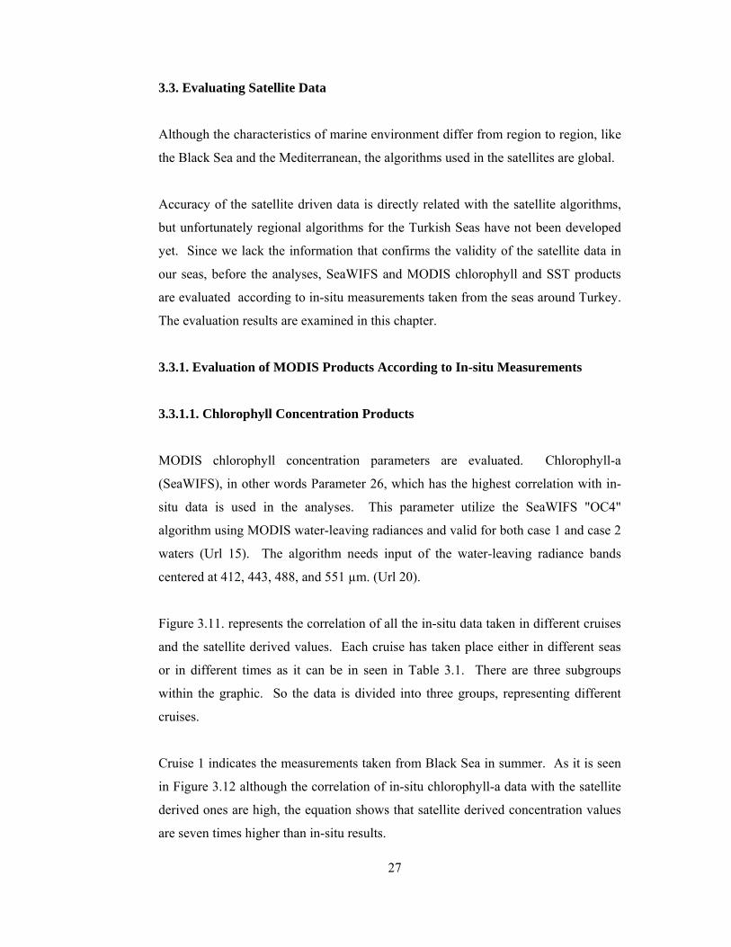
34
Satellite derived SEAWIFS chlorophyll_a concentration values versus in_situ
measurements in the third cruise in the Black Sea is given in Figure 3.20.
Cruise 3
y = 2.9362xR2 = 0.5383
0
1
2
3
0 1 2 3
In-situ Chlor(tot)
SEA
WIF
S C
hlor
Figure 3.20. Satellite Derived SEAWIFS Chlorophyll_a Concentration Values
Versus In_situ Measurements in the Third Cruise
The graphical representation of Cruise 5 is not given in the thesis due the insufficient
number of satellite derived SEAWIFS chlorophyll_a concentration values versus
in_situ measurements.
3.3.2.2. Sea Surface Temperature Products
LAC Level-1A products were analyzed in SeaDAS software to generate the SST
parameters. SeaWIFS parameter shows high correlation with the in-situ data as
indicated in Figure 3.21. This dataset includes both Black Sea and Mediterranean so
the data is divided into two to check the algorithm in each sea.
Figure 3.21 represents the correlation between satellite derived SEAWIFS SST
values and the in-situ measurements. Although MODIS algorithm yields better
results, the correlation coefficient is high.

35
Cruise 1/3/5 y = 1.0068xR2 = 0.6614
171819202122232425
17 18 19 20 21 22 23 24 25
In-situ SST
SEA
WIF
S SS
T
Figure 3.21. Satellite Derived SEAWIFS SST Values Versus In_situ Measurements
In-situ values for Black Sea are taken in two different seasons, summer and autumn.
SeaWIFS SST parameter has overestimated the in-situ values in summer like
MODIS sst 4 parameter and underestimate them in winter. The representation of the
Black Sea and Mediterranean cruises are given in Figure 3.22 and Figure 3.23
respectively.
Cruise 1/3
y = 1.0129xR2 = 0.7366
171819202122232425
17 18 19 20 21 22 23 24 25
In-situ SST
SEA
WIF
S SS
T
Figure 3.22. Satellite Derived SEAWIFS SST Values Versus In_situ Measurements
in the Black Sea.
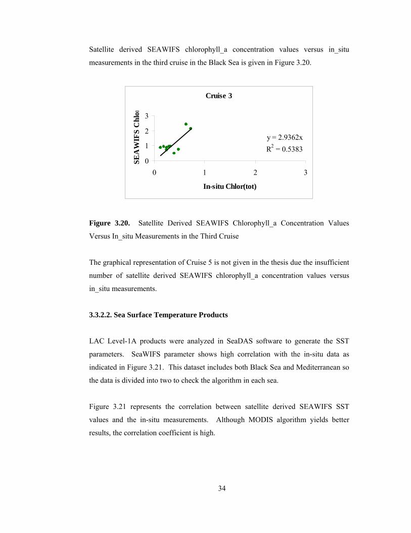
SST measurements seem to have a good correlation with the in-situ values in the
Mediterranean, but the numbers of the in-situ measurements are not enough as given
in Figure 3.23.
36
Cruise 5
y = 1.0622xR2 = 0.6805
17
19
21
23
25
27
17 18 19 20 21 22 23 24
In-situ SSTSE
AW
IFS
SST
Figure 3.23. Satellite Derived SEAWIFS SST Values Versus In_situ Measurements
in the Mediterranean.
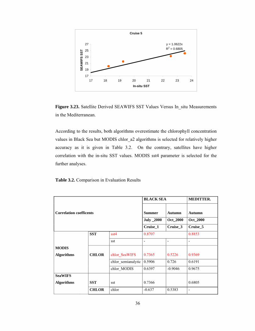
According to the results, both algorithms overestimate the chlorophyll concentration
values in Black Sea but MODIS chlor_a2 algorithms is selected for relatively higher
accuracy as it is given in Table 3.2. On the contrary, satellites have higher
correlation with the in-situ SST values. MODIS sst4 parameter is selected for the
further analyses.
Table 3.2. Comparison in Evaluation Results
BLACK SEA MEDITTER.
Correlation coefficents Summer Autumn Autumn
July _2000 Oct_2000 Oct_2000
Cruise_1 Cruise_3 Cruise_5
SST sst4 0.8707 0.8853
sst - - -
MODIS
Algorithms CHLOR chlor_SeaWIFS 0.7365 0.5226 0.9369
chlor_semianalytic 0.5906 0.726 0.6191
chlor_MODIS 0.6397 -0.9046 0.9675
SeaWIFS
Algorithms SST sst 0.7366 0.6805
CHLOR chlor -0.637 0.5383 -

37
In Table 3.3 first two columns in the charts indicate Julian dates of the images
utilized in the analyses. Real Julian dates indicate the day imagery is collected. If
the image is absent or the necessary part is covered with cloud, instead of that, the
imagery collected on the next day, which is represented in used column is utilized.
As it is seen from the table due to the absence of SeaWIFS imagery and high cloud
ratio, most of the calculations are done within ± 1 day interval. This is also a
disadvantage for the accurate comparison of the algorithms.
Table 3.3. Dates of Satellite Imagery Used for the Evaluation.
a) SEAWIFS imagery b)MODIS imagery
a)
b)

38
CHAPTER 4
ANALYSES
4.1. Description of Interannual Environmental Variability in Black Sea
Black Sea is the largest landlocked basin in the world. It is connected to the Azov
Sea through the Kerch Straits and to the Marmara Sea with a restricted exchange
through the Bosphorous and Dardanellas Straits (Beşiktepe et al., 2001; Özsoy and
Ünlüata, 1997).
Due to the increased nutrient input via major rivers during the last few decades,
Black Sea ecosystem has been subject to changes in recent years. Intrusion of new
species (a lobate ctenophore, Mnemiopsis sp.) into the Black Sea, which competes
with Anchovy for the zooplankton and morever consuming anchovy eggs and
larvae in the Black Sea has resulted a decline in the Anchovy and other pelagic fish
stocks (Kıdeys, 1994).
The major rivers discharging into the Black Sea are Danube, Dpener and Dnester.
Danube alone holds the 50 % of the river run-off, which is 3 times higher than the
total discharge of the Dneper and Dnester (Özsoy and Ünlüata, 1997).
Due to the sediment and nutrient load, river discharges has distinct effects on the
Black Sea, which are sediment load directly affecting the water properties, whereas
the nutrients have an indirect effect by inducing the planktonic flora. Both processes
can be evaluated via the satellite imagery (Barale et al., 2002).
Besides the freshwater inputs from the rivers, Black Sea is also influenced by
atmospheric effects, fluxes through straits and changes in topography. The

39
circulation of the Black Sea need to be observed for understanding of primary
production, growth and migration of the pelagic marine organisms (Özsoy and
Ünlüata, 1997).
According to Besiktepe et al., (2001), the upper layer circulation is characterized by
a cyclonic circulation in the center of the basin, which is stronger over the
continental slope. Center region circulation is composed of weak cyclonic eddies
and smaller and weaker anticyclones. In the outer boundary of the central cyclonic
region and over the continental slope, there is a strong current called the Rim
Current. On the coastal side of the Rim Current there are a series of anticyclonic
eddies and the largest anticyclonic gyre is the Batumi gyre. It is often possible to
identify eddies with their temperature pattern, since center of the anticyclones are
usually cooler than their surroundings. Rim current can be divided into segments
according to the different structural characteristics. Figure 4.1 represents the general
circulation pattern of the Black Sea.
Northwest Shelfbreak Current, starts from Crimea Peninsula and reaches Bosphorous
Strait in the North. It consists of two semi-permanent anticyclonic eddies, Sevastopol
Eddy in the North and Kaliakra Eddy in the South.The driving mechanism is
influenced by fresh water entrance and wind effect respectively.
Anatolian current, lies along the anatolian coast. Three to five anticyclonic cells with
different strenghts are present on the shoreward side of the current. One of which is
the Sakarya Eddy. Caucasian-Kerch Current, covers the rest of the Black Sea from
the Battumi Gyre to the Crimea Peninsula and leads the formation of the caucasian
eddy.
MODIS 8 day composite Level 3 Chlorophyll concentration and SST images starting
from the end of February 2000 and continues to the middle of March 2001 are given
in Appendix I. The given imagery might be used for visual interpretation of upper
layer circulation pattern and the interannual variability in terms of change in
chlorophyll concentration and SST.

40
a
b
c
Figure 4.1. a) Representation of the upper layer general circulation pattern of the
Black Sea. After Oğuz et al. (1993). b) MODIS L3 chlorophyll concentration
imagery (24May-31May) c) MODIS L3 chlorophyll conc. imagery overlaid by
circulation pattern
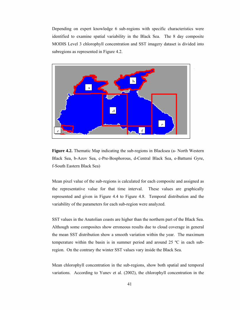
41
Depending on expert knowledge 6 sub-regions with specific characteristics were
identified to examine spatial variability in the Black Sea. The 8 day composite
MODIS Level 3 chlorophyll concentration and SST imagery dataset is divided into
subregions as represented in Figure 4.2.
1
Figure 4.2. Thematic Map indicating the sub-regions in Blacksea (a- North Western
Black Sea, b-Azov Sea, c-Pre-Bosphorous, d-Central Black Sea, e-Battumi Gyre,
f-South Eastern Black Sea)
Mean pixel value of the sub-regions is calculated for each composite and assigned as
the representative value for that time interval. These values are graphically
represented and given in Figure 4.4 to Figure 4.8. Temporal distribution and the
variability of the parameters for each sub-region were analyzed.
SST values in the Anatolian coasts are higher than the northern part of the Black Sea.
Although some composites show erroneous results due to cloud coverage in general
the mean SST distribution show a smooth variation within the year. The maximum
temperature within the basin is in summer period and around 25 ºC in each sub-
region. On the contrary the winter SST values vary inside the Black Sea.
Mean chlorophyll concentration in the sub-regions, show both spatial and temporal
variations. According to Yunev et al. (2002), the chlorophyll concentration in the
ab
d
efc

42
Black Sea reaches peak values in winter and spring, the maximum occurs in January
and March and a less marked peak is seen in November. However the values
gathered from MODIS imagery reveals that the peak concentrations are in spring, or
summer and autumn mainly in March, June and November.
Daskalov (1998), states that due to the impact of low temperatures and strong winds
in winter time, the shelf zone is subject to intensive vertical mixing. Thus the
phytoplankton bloom begins in the open sea in February-March accompanied by a
zooplankton bloom in spring. The plankton bloom in the shallow North Western
Shelf is generally delayed to the warmer season because of the more intensive winter
cooling. It is also strengthened by the high river discharge in May and June.

43
i- North-western shelf
Although the outcome of the MODIS imagery interpretation gives similar results as
Daskalov, unfortunately the chlorophyll concentration values in the North Western
Shelf (Figure 4.3) and Azov Sea (Figure 4.4) are highly overestimated. The results
might be influenced by the high freshwater inflow carrying both sediment and
nutrients into these regions. In the shelf area SST ranges between 5 to 11 ºC (Figure
4.4).
a)
0123456789
10
5Mar
-13M
ar
21M
ar-2
9Mar
6Apr
-14A
pr
22Ap
r-30
Apr
8May
-16M
ay
24M
ay-1
Jun
9Jun
-17J
un
25Ju
n-3J
un
11Ju
n-19
jun
27Ju
n-20
Aug
28Au
g-5S
ep
13Se
p-21
Sep
29Se
p-7O
ct
15O
ct-2
3Oct
31O
ct-8
Nov
16N
ov-2
4Nov
2Dec
-10D
ec
18D
ec-2
6Dec
3Jan
-11J
an
19Ja
n-27
Jan
4Feb
-12F
eb
20Fe
b-28
Feb
8Mar
-16M
ar
Date
MO
DIS
Chl
orop
hyll_
a C
once
ntra
tion
(mg/
m3)
b)
4
9
14
19
24
26Fe
b-5M
ar
13M
ar-2
1Mar
29M
ar-6
Apr
14A
pr-2
2Apr
30A
pr-8
May
16M
ay-2
4May
1Jun
-9Ju
n
17Ju
n-25
Jun
3Jun
-11J
un
19ju
n-27
Jun
20A
ug-2
8Aug
5Sep
-13S
ep
21S
ep-2
9Sep
7Oct
-15O
ct
23O
ct-3
1Oct
8Nov
-16N
ov
24N
ov-2
Dec
10D
ec-1
8Dec
26D
ec-3
Jan
11Ja
n-19
Jan
27Ja
n-4F
eb
12Fe
b-20
Feb
28Fe
b-8M
ar
Date
MO
DIS
SST
(ºC
)
Figure 4.3. a) Annual Mean Chlorophyll-a Distribution of North Western Shelf
b)Annual Mean SST Distribution of North Western Shelf
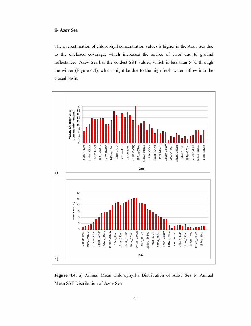
44
ii- Azov Sea
The overestimation of chlorophyll concentration values is higher in the Azov Sea due
to the enclosed coverage, which increases the source of error due to ground
reflectance. Azov Sea has the coldest SST values, which is less than 5 ºC through
the winter (Figure 4.4), which might be due to the high fresh water inflow into the
closed basin.
a)
02468
101214161820
5Mar
-13M
ar
21M
ar-2
9Mar
6Apr
-14A
pr
22A
pr-3
0Apr
8May
-16M
ay
24M
ay-1
Jun
9Jun
-17J
un
25Ju
n-3J
un
11Ju
n-19
jun
27Ju
n-20
Aug
28A
ug-5
Sep
13S
ep-2
1Sep
29S
ep-7
Oct
15O
ct-2
3Oct
31O
ct-8
Nov
16N
ov-2
4Nov
2Dec
-10D
ec
18D
ec-2
6Dec
3Jan
-11J
an
19Ja
n-27
Jan
4Feb
-12F
eb
20Fe
b-28
Feb
8Mar
-16M
ar
Date
MO
DIS
Chl
orop
hyll_
a Co
ncen
tratio
n (m
g/m
3)
b)
0
5
10
15
20
25
30
26Fe
b-5M
ar
13M
ar-2
1Mar
29M
ar_6
Apr
14A
pr_2
2Apr
30A
pr_8
May
16M
ay_2
4May
1Jun
_9Ju
n
17Ju
n_25
Jun
3Jun
_11J
un
19ju
n_27
Jun
20Au
g_28
Aug
5Sep
_13S
ep
21S
ep_2
9Sep
7Oct
_15O
ct
23O
ct_3
1Oct
8Nov
_16N
ov
24N
ov_2
Dec
10D
ec_1
8Dec
26D
ec_3
Jan
11Ja
n_19
Jan
27Ja
n_4F
eb
12Fe
b_20
Feb
28Fe
b_8M
ar
Date
MO
DIS
SST
(ºC
)
Figure 4.4. a) Annual Mean Chlorophyll-a Distribution of Azov Sea b) Annual
Mean SST Distribution of Azov Sea

45
iii- Pre-Bosphorous
The rest of the sub-regions are mostly free from strong outer effects. Pre-bosphorous
(Figure 4.5) show peak concentrations in late-spring/summer (May-June) and
autumn (November). The area is warmer relative to the Northern Part, and the
temperature varies between 7 to 11ºC.
a)
0
0.5
1
1.5
2
2.5
3
5Mar
-13M
ar
21M
ar-2
9Mar
6Apr
-14A
pr
22A
pr-3
0Apr
8May
-16M
ay
24M
ay-1
Jun
9Jun
-17J
un
25Ju
n-3J
un
11Ju
n-19
jun
27Ju
n-20
Aug
28A
ug-5
Sep
13S
ep-2
1Sep
29S
ep-7
Oct
15O
ct-2
3Oct
31O
ct-8
Nov
16N
ov-2
4Nov
2Dec
-10D
ec
18D
ec-2
6Dec
3Jan
-11J
an
19Ja
n-27
Jan
4Feb
-12F
eb
20Fe
b-28
Feb
8Mar
-16M
ar
Date
MO
DIS
Chl
orop
hyll_
a Co
ncen
tratio
n (m
g/m
3)
b)
0
5
10
15
20
25
30
26Fe
b-5M
ar
13M
ar-2
1Mar
29M
ar-6
Apr
14A
pr-2
2Apr
30A
pr-8
May
16M
ay-2
4May
1Jun
-9Ju
n
17Ju
n-25
Jun
3Jun
-11J
un
19ju
n-27
Jun
20Au
g-28
Aug
5Sep
-13S
ep
21S
ep-2
9Sep
7Oct
-15O
ct
23O
ct-3
1Oct
8Nov
-16N
ov
24N
ov-2
Dec
10D
ec-1
8Dec
26D
ec-3
Jan
11Ja
n-19
Jan
27Ja
n-4F
eb
12Fe
b-20
Feb
28Fe
b-8M
ar
Date
MO
DIS
SST
(ºC
)
Figure 4.5. a) Annual Mean Chlorophyll-a Distribution of Pre_Bosphorous
b) Annual Mean SST Distribution of Pre_Bosphorous

46
iv- Central Black Sea
Central Black Sea shows similarity with the Pre-bosphorous. As represented in
Figure 4.6, peak concentrations are in late-spring/summer (May-June) and autumn
(November) and the temperature varies between 7 to 11ºC .
a)
0.2
0.4
0.6
0.8
1
1.2
1.4
5Mar
-13M
ar
21M
ar-2
9Mar
6Apr
-14A
pr
22A
pr-3
0Apr
8May
-16M
ay
24M
ay-1
Jun
9Jun
-17J
un
25Ju
n-3J
un
11Ju
n-19
jun
27Ju
n-20
Aug
28A
ug-5
Sep
13S
ep-2
1Sep
29S
ep-7
Oct
15O
ct-2
3Oct
31O
ct-8
Nov
16N
ov-2
4Nov
2Dec
-10D
ec
18D
ec-2
6Dec
3Jan
-11J
an
19Ja
n-27
Jan
4Feb
-12F
eb
20Fe
b-28
Feb
8Mar
-16M
ar
Date
MO
DIS
Chlo
roph
yll_
a Co
ncen
tratio
n (m
g/m
3)
b)
4
9
14
19
24
26Fe
b-5M
ar
13M
ar-2
1Mar
29M
ar-6
Apr
14A
pr-2
2Apr
30A
pr-8
May
16M
ay-2
4May
1Jun
-9Ju
n
17Ju
n-25
Jun
3Jun
-11J
un
19ju
n-27
Jun
20A
ug-2
8Aug
5Sep
-13S
ep
21S
ep-2
9Sep
7Oct
-15O
ct
23O
ct-3
1Oct
8Nov
-16N
ov
24N
ov-2
Dec
10D
ec-1
8Dec
26D
ec-3
Jan
11Ja
n-19
Jan
27Ja
n-4F
eb
12Fe
b-20
Feb
28Fe
b-8M
ar
Date
MO
DIS
SST
(ºC
)
Figure 4.6. a) Annual Mean Chlorophyll-a Distribution of Central Black Sea
b) Annual Mean SST Distribution of Central Black Sea

47
v- Battumi Gyre
The Eastern part of the Black Sea, Battumi gyre (Figure 4.7) has the highest
concentration values in spring (March) and autumn (November). Also the Eastern
part is the warmest during the winter period is where the SST is around 8 to 12 º C
SST.
a)
0.5
1
1.5
2
2.5
5Mar
-13M
ar
21M
ar-2
9Mar
6Apr
-14A
pr
22A
pr-3
0Apr
8May
-16M
ay
24M
ay-1
Jun
9Jun
-17J
un
25Ju
n-3J
un
11Ju
n-19
jun
27Ju
n-20
Aug
28A
ug-5
Sep
13S
ep-2
1Sep
29S
ep-7
Oct
15O
ct-2
3Oct
31O
ct-8
Nov
16N
ov-2
4Nov
2Dec
-10D
ec
18D
ec-2
6Dec
3Jan
-11J
an
19Ja
n-27
Jan
4Feb
-12F
eb
20Fe
b-28
Feb
8Mar
-16M
ar
Date
MO
DIS
Chl
orop
hyll_
a C
once
ntra
tion
(mg/
m3)
b)
468
1012141618202224
26Fe
b-5M
ar
13M
ar-2
1Mar
29M
ar-6
Apr
14A
pr-2
2Apr
30A
pr-8
May
16M
ay-2
4May
1Jun
-9Ju
n
17Ju
n-25
Jun
3Jun
-11J
un
19ju
n-27
Jun
20A
ug-2
8Aug
5Sep
-13S
ep
21S
ep-2
9Sep
7Oct
-15O
ct
23O
ct-3
1Oct
8Nov
-16N
ov
24N
ov-2
Dec
10D
ec-1
8Dec
26D
ec-3
Jan
11Ja
n-19
Jan
27Ja
n-4F
eb
12Fe
b-20
Feb
28Fe
b-8M
ar
Date
MO
DIS
SST
(ºC
)
Figure 4.7. a) Annual Mean Chlorophyll-a Distribution of Battumi Gyre b) Annual
Mean SST Distribution of Battumi Gyre

48
vi- South-Eastern Blacksea
South-Eastern Blacksea is similar to the Battumi gyre, the area shows the highest
concentration values in spring (March) and autumn (November) as given in Figure
4.8. During the winter period the SST is around 8 to 12 º C SST in South Eastern
Black Sea (4.8) similar to the the Battumi gyre (Figure 4.7).
a)
0.5
1
1.5
2
5Mar
-13M
ar
21M
ar-2
9Mar
6Apr
-14A
pr
22A
pr-3
0Apr
8May
-16M
ay
24M
ay-1
Jun
9Jun
-17J
un
25Ju
n-3J
un
11Ju
n-19
jun
27Ju
n-20
Aug
28A
ug-5
Sep
13S
ep-2
1Sep
29S
ep-7
Oct
15O
ct-2
3Oct
31O
ct-8
Nov
16N
ov-2
4Nov
2Dec
-10D
ec
18D
ec-2
6Dec
3Jan
-11J
an
19Ja
n-27
Jan
4Feb
-12F
eb
20Fe
b-28
Feb
8Mar
-16M
ar
Date
MO
DIS
Chl
orop
hyll_
a C
once
ntra
tion
(mg/
m3)
b)
468
1012141618202224
26Fe
b-5M
ar
13M
ar-2
1Mar
29M
ar-6
Apr
14A
pr-2
2Apr
30A
pr-8
May
16M
ay-2
4May
1Jun
-9Ju
n
17Ju
n-25
Jun
3Jun
-11J
un
19ju
n-27
Jun
20A
ug-2
8Aug
5Sep
-13S
ep
21S
ep-2
9Sep
7Oct
-15O
ct
23O
ct-3
1Oct
8Nov
-16N
ov
24N
ov-2
Dec
10D
ec-1
8Dec
26D
ec-3
Jan
11Ja
n-19
Jan
27Ja
n-4F
eb
12Fe
b-20
Feb
28Fe
b-8M
ar
Date
MO
DIS
SST
(ºC
)
Figure 4.8. a) Annual Mean Chlorophyll_a Distribution of South Eastern Blacksea
b) Annual Mean SST Distribution of South Eastern Blacksea

49
4.2. Determination of Potential Favorable Zones for Pelagic Fish Stocks in the
Black Sea
The capabilities of GIS, like managing large amounts of spatial data and also the
ability to integrate multiple layers and ancillary data, have made GIS an effective
tool in defining potential favorable zones for fish stocks. However for the
integration of decision maker’s preferences and the geographical data, a combination
of GIS and MCDA is needed.
Two different decision rules are employed to generate fish stock maps, simple
additive weigthing (SAW) and fuzzy additive weigthing (FSAW). These methods
are similar, such that they both use the weighted average as the aggregation operator.
However FSAW methods utilizes fuzzy data (Malczewski, 1999).
4.2.1. Determination of Potential Favorable Zones using SAW
A weight value that indicates the criterion importance relative to the other criteria is
assigned to each criterion. Each criterion is ranked according to the decision maker’s
preferences. This criterion weighting method is called the ranking method and
preferred due to its simplicity to apply (Malczewski, 1999).
Two criteria of equal importance (SST and chlorophyll concentration) are defined for
this application. Each layer representing the criteria is divided into classes and given
rank values according to their importance. Images are then reclassified upon the
assigned rank values. The preferred temperature interval and the chlorophyll
concentration for the anchovy are obtained from the literature.
In the literature there are only a few sea surface temperature measurements for the
Black Sea Anchovy. Using the definitions in the literature, different temperature
intervals are defined for different seasonal periods. During the spawning period for
Anchovy starting from the end of April till the beginning of September fishing is
prohibited in Black Sea. Thus this period is neglected in the analyses. Each
temperature interval that is defined covers 3 ºC and has a 1ºC overlap with the

50
neighbouring intervals. These intervals are assumed to be the best potential
temperatures for the assigned seasonal periods and they are used as basis in the
further analyses.
Weight assigned for each layer is multiplied by the rank value given to each class
and all the overall scores are calculated. The zone with the highest score is chosen to
be the best potential area. This method is named as SAW in the literature (Thill,
1999).
4.2.1.1. Sea Surface Temperature Images
Five different temperature intervals are defined according to the temperature
preferences of Anchovy in the literature and expert knowledge as it is shown in the
Figure 4.9. Each temperature interval is given the highest rank values in the assigned
seasonal periods. For example SST imagery captured on 3rd of January 2001
belongs to 11-14 ºC temperature interval group. Pixel values within this range take 5
points out of 5. The neighbouring temperature intervals 14-16 ºC and 9-11 ºC are
given 4 as rank value. Successive intervals take the lower values as they diverge
from the prefered temperature values.
Figure 4.9. Mean SST Distribution Throughout the Black Sea and the Temperature
Intervals

51
It should also be considered that although the Level 3 products are 8 day composite,
the imagery captured especially on winter may contain inaccurate results or null
values due to cloud coverage.
The reclassification results are given in the Figure 4.10. Prefered temperature
interval having highest rank value is indicated in red color and the areas having
lowest rank value are indicated in dark blue color.

52
26 February - 4 March
5 March - 12 March
13 March - 20 March
21 March - 28 March
29 March - 5 April
6 April - 13 April
14 April - 21 April
22 April - 29 April
Lowest Highest
Figure 4.10. Reclassified SST Distribution in Black Sea

53
5 September - 12 September
13 September - 20 September
21 September - 28 September
29 September - 6 October
7 October - 14 October
15 October - 22 October
23 October - 30 October
31 October - 7 November
Lowest Highest
Figure 4.10. (continued). Reclassified SST Distribution in Black Sea

54
8 November – 15 November
16 November – 23 November
24 November – 1 December
2 December – 9 December
10 December – 17 December
18 December – 25 December
26 December – 2 January
3 January – 10 January
Lowest Highest
Figure 4.10. (continued). Reclassified SST Distribution in Black Sea

55
11 January – 18 January
19 January - 26 January
27 January – 3 February
4 February – 11 February
12 February – 19 February
20 February – 27 February
28 February – 7 March
8 March – 15 March
Lowest Highest
Figure 4.10. (continued). Reclassified SST Distribution in Black Sea

56
4.2.1.2. Chlorophyll Concentration Images
MODIS Level 3 Chlorophyll concentration images are reclassified according to the
availability of nutrient. As it it clearly seen from the reclassified chlorophyll
concentration imagery in Figure 4.11, rivers flowing into the Black Sea are important
source of nutrient. Especially the large rivers in the North West keep the
concentration values high in the coast throughout the year. Also Azov Sea has high
concentration during the year without exception, due to inflow of the river Don and
its enclosed coverage.
Assuming that the anchovy would prefer to be in the zones having nutrient, the
imagery is reclassified according to the chlorophyll concentration values. The
concentration between 20-5 mg/m3 is given the highest rank value and as the
concentration decreases, the rank values decreases sucessively. Whereas
Chlorophyll concentrations more than 20 mg/m3 is assumed to be too much and/or
erroneous values (Yunev, 2002) so concentrations more than this value is given the
lowest rank value. As an example, a pixel having a concentration value of 6 mg/m3
takes the highest rank value 5 out of 5, and if the value is between 3 to 5 mg/m3 the
corresponding rank value is 4.
In reclassified chlorophyll concentration images red areas indicates highest rank
value and the lowest rank value areas are represented by dark blue color.

57
26 February – 4 March
5 March – 12 March
13 March – 20 March
21 March – 28 March
29 March – 5 April
6 April – 13 April
14 April – 21 April
22 April – 29 April
Lowest Highest
Figure 4.11. Reclassified Chlorophyll Concentration Distribution in Black Sea

58
5 September – 12 September
13 September – 20 September
21 September – 28 September
29 September – 6 October
7 October – 14 October
15 October – 22 October
23 October - 30 October
31 October – 7 November
Lowest Highest
Figure 4.11. (continued). Reclassified Chlorophyll Concentration Distribution in
Black Sea

59
8 November – 15 November
16 November – 23 November
24 November – 1 December
2 December – 9 December
10 December – 17 December
18 December – 25 December
26 December – 2 January
3 January – 10 January
Lowest Highest
Figure 4.11. (continued). Reclassified Chlorophyll Concentration Distribution in
Black Sea
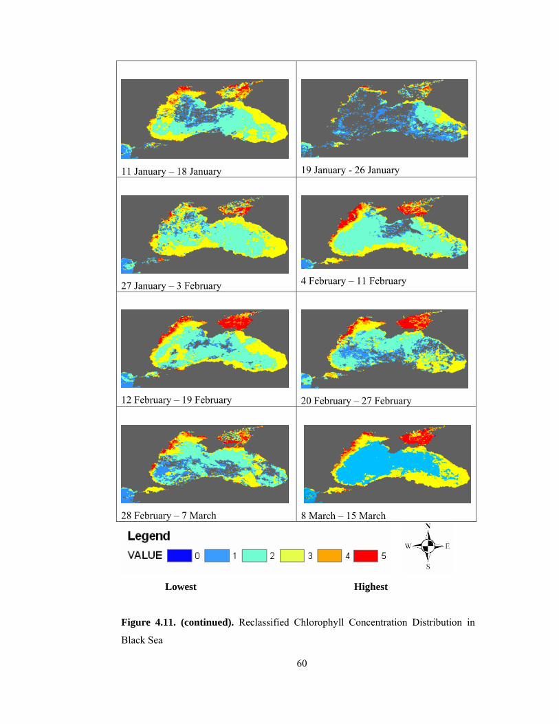
60
11 January – 18 January
19 January - 26 January
27 January – 3 February
4 February – 11 February
12 February – 19 February
20 February – 27 February
28 February – 7 March
8 March – 15 March
Lowest Highest
Figure 4.11. (continued). Reclassified Chlorophyll Concentration Distribution in
Black Sea

61
4.2.1.3. Resultant Thematic Fish Stock Maps Generated by SAW
Reclassified images of SST and chlorophyll concentration are assigned equal weight
values due to assumption that each layer has equal contribution to define fish stock
maps. SST is known be the most significant parameter which defines the fish
habitat, and the accuracy of satellite derived SST values are higher with respect to
the cholorophyll concentration values. Yet still it is assumed that both the
temperature and nutrient availabilty affect the habitat of fish and equal weight values
are used to overcome the domination of SST values over cholorophyll concentration
values.
The reclassified layers are summed and the zone with the highest score is chosen to
be the potential favorable zones.
The resultant maps are given in the 4.12. Parallel to the literature, potential favorable
zones for anchovy are located on the Northern part of the Black Sea in the end of
summer and the beginning of autumn. As the winter approaches the potential sites
start to approach south to warmer waters and reach Turkish coasts.

62
26 February – 4 March
5 March – 12 March
13 March – 20 March
21 March – 28 March
29 March – 5 April
6 April – 13 April
14 April – 21 April
22 April – 29 April
Lowest Highest
Figure 4.12. Resultant Thematic Fish Stock Maps Generated by SAW in Black Sea

63
5 September – 12 September
13 September – 20 September
21 September – 28 September
29 September – 6 October
7 October – 14 October
15 October – 22 October
23 October – 30 October
31 October – 7 November
Lowest Highest
Figure 4.12. (continued). Resultant Thematic Fish Stock Maps Generated by SAW

64
8 November – 15 November
16 November – 23 November
24 November – 1 December
2 December – 9 December
10 December – 17 December
18 December – 25 December
26 December – 2 January
3 January – 10 January
Lowest Highest
Figure 4.12. (continued). Resultant Thematic Fish Stock Maps Generated by SAW

65
11 January – 18 January
19 January – 26 January
27 January – 3 February
4 February – 11 February
12 February – 19 February
20 February – 27 February
28 February – 7 March
8 March – 15 March
Lowest Highest
Figure 4.12. (continued). Resultant Thematic Fish Stock Maps Generated by SAW

66
4.2.2. Determination of Potential Favorable Zones using FSAW
The capability of SAW and GIS application combination which utilize classical set
theory are inadequate to interpret the natural variability in the environment. The
other method applied to generate fish stock maps is the integration of FSAW and
GIS.
Fuzzy sets provides powerful representation of critical components of spatial
decision making and furthermore a meaningful representation of vague or imprecise
concepts (Malczewski,1999).
Through the use of linguistic variables, experts experiences involving imprecision,
are converted to fuzzy rules. In this thesis, the fuzzy analyses are implemented on
FuzzyCell software, which is developed on a commercial GIS software called
ArcMap. This is free software and developed at METU Geodetic and Geographic
Information Technologies Department. FuzzyCell allows users to handle imprecision
in the decision making process (Yanar and Akyürek, 2005).

67
4.2.2.1. Sea Surface Temperature Images
MODIS Level 3 images and the previously defined temperature intervals are used in
the analyses. As each temperature interval is given the highest rank values in the
reclassification process, again in the membership function of fuzzy logic analyses
prefered temperature interval is given the peak values for the assigned seasonal
period. Bell shaped membership function, which is believed to define the smooth
transition between the class values as given in the Figure 4.13, is selected to define
the SST.
The areas, which suits the habitat preferences of anchovy are indicated in red and the
least prefered areas are shown in dark blue color as given in Figure 4.14.
Figure 4.13. Bell Shaped Membership Function Defining the SST Distribution in
Black Sea.

68
26 February – 4 March
5 March – 12 March
13 March – 20 March
21 March – 28 March
29 March – 5 April
6 April – 13 April
14 April – 21 April
22 April – 29 April
Figure 4.14. Reclassified SST Distribution in Black Sea with Bell Shaped
Membership Function

69
5 September – 12 September
13 September – 20 September
21 September – 28 September
29 September – 6 October
7 October – 14 October
15 October – 22 October
23 October – 30 October
31 October – 7 November
Figure 4.14. (continued). Reclassified SST Distribution in Black Sea with Bell
Shaped Membership Function

70
8 November – 15 November
16 November – 23 November
24 November – 1 December
2 December – 9 December
10 December – 17 December
18 December – 25 December
26 December – 2 January
3 January – 10 January
Figure 4.14. (continued). Reclassified SST Distribution in Black Sea with Bell
Shaped Membership Function
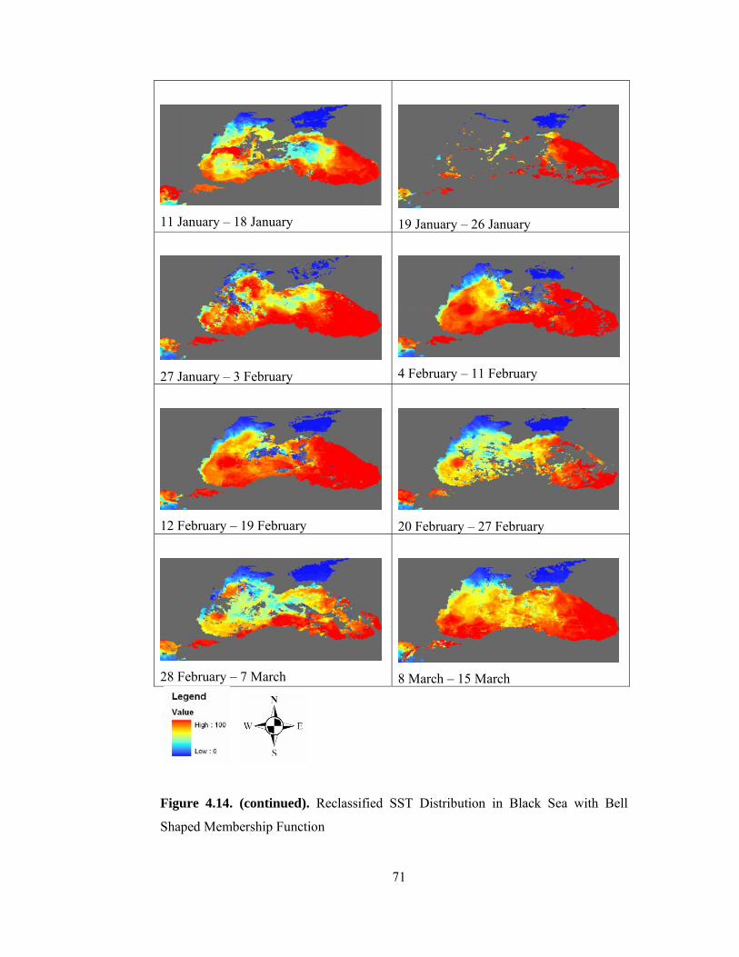
71
11 January – 18 January
19 January – 26 January
27 January – 3 February
4 February – 11 February
12 February – 19 February
20 February – 27 February
28 February – 7 March
8 March – 15 March
Figure 4.14. (continued). Reclassified SST Distribution in Black Sea with Bell
Shaped Membership Function

72
4.2.2.2. Chlorophyll Concentration Images
Several trials are performed and finally trapezoidal membership function is believed
to define the nutrient availability from MODIS Level 3 Chlorophyll concentration
images. The concentration values between 5-20 mg/m3 is given the highest value in
the function and the values decrease linearly as the concentration decreases.
Chlorophyll concentrations more than 20 mg/m3 is assumed to be too much and/or
erroneous values so concentrations more than this value are given lower values as the
concentration increases.
The chlorophyll concentration having highest values are indicated in red color color
and the lowest value areas are indicated in dark blue color. The reclassified
chlorophyll concentration distribution in Black Sea in Figure 4.11 is mainly similar
to the reclassified maps in Figure 4.16. The chlorophyll concentration in the North
Eastern Black Sea and the Azov Sea are high throughout the year.
Figure 4.15. Trapezoidal Membership Function Defining the Chlorophyll
Concentration Distribution in Black Sea.

73
26 February – 4 March
5 March – 12 March
13 March – 20 March
21 March – 28 March
29 March – 5 April
6 April – 13 April
14 April – 21 April
22 April – 29 April
Figure 4.16. Chlorophyll Concentration Distribution in Black Sea

74
5 September – 12 September
13 September – 20 September
21 September – 28 September
29 September – 6 October
7 October – 14 October
15 October – 22 October
23 October – 30 October
31 October – 7 November
Figure 4.16. (continued). Reclassified Chlorophyll Concentration Distribution in
Black Sea with Trapezoidal Membership Function.

75
8 November – 15 November
16 November – 23 November
24 November – 1 December
2 December – 9 December
10 December – 17 December
18 December – 25 December
26 December – 2 January
3 January – 10 January
Figure 4.16. (continued). Reclassified Chlorophyll Concentration Distribution in
Black Sea with Trapezoidal Membership Function.
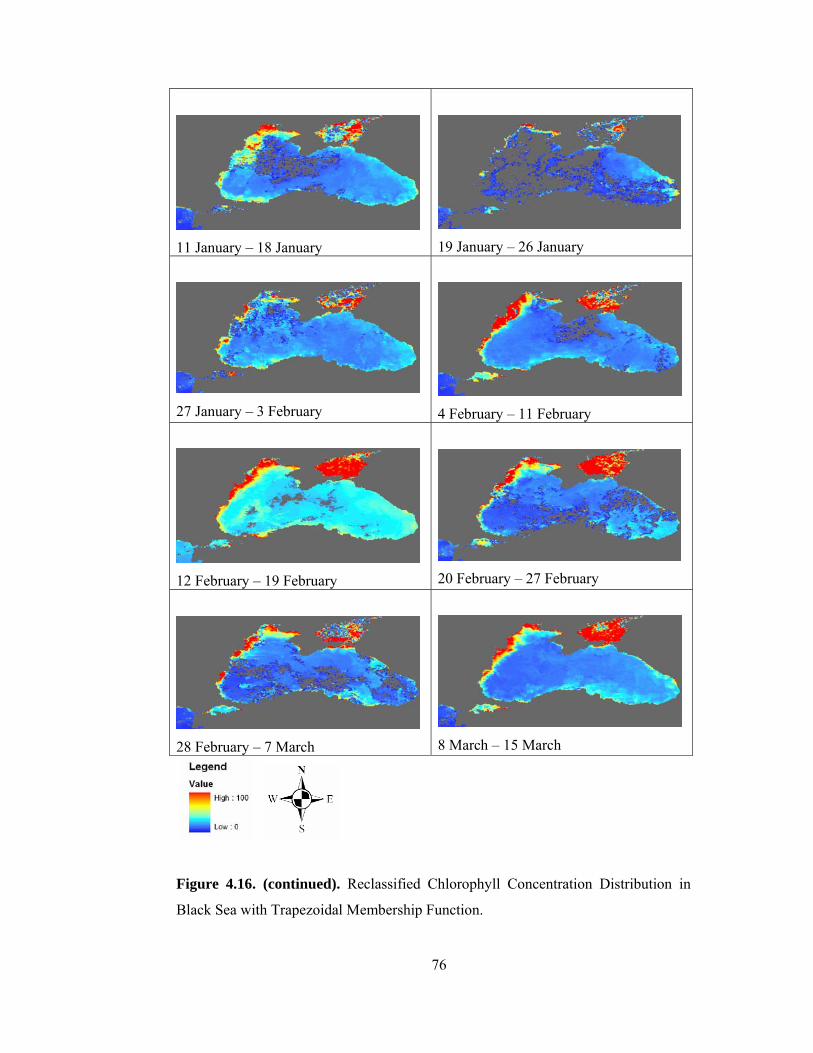
76
11 January – 18 January
19 January – 26 January
27 January – 3 February
4 February – 11 February
12 February – 19 February
20 February – 27 February
28 February – 7 March
8 March – 15 March
Figure 4.16. (continued). Reclassified Chlorophyll Concentration Distribution in
Black Sea with Trapezoidal Membership Function.
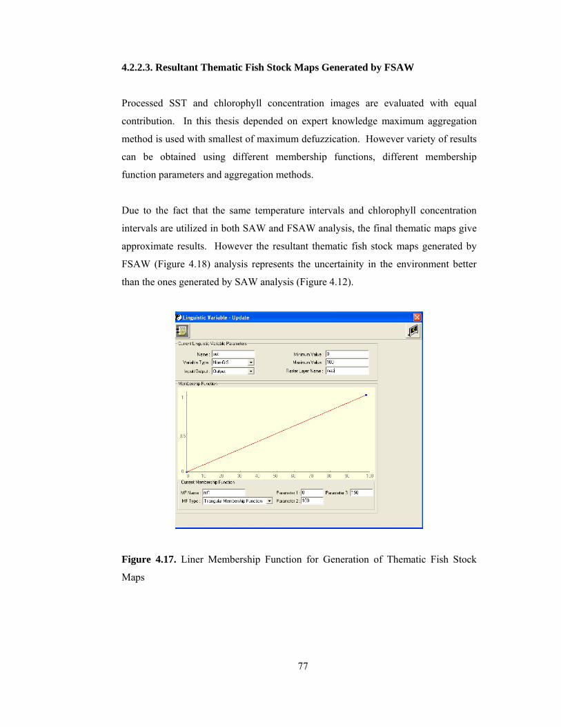
77
4.2.2.3. Resultant Thematic Fish Stock Maps Generated by FSAW
Processed SST and chlorophyll concentration images are evaluated with equal
contribution. In this thesis depended on expert knowledge maximum aggregation
method is used with smallest of maximum defuzzication. However variety of results
can be obtained using different membership functions, different membership
function parameters and aggregation methods.
Due to the fact that the same temperature intervals and chlorophyll concentration
intervals are utilized in both SAW and FSAW analysis, the final thematic maps give
approximate results. However the resultant thematic fish stock maps generated by
FSAW (Figure 4.18) analysis represents the uncertainity in the environment better
than the ones generated by SAW analysis (Figure 4.12).
Figure 4.17. Liner Membership Function for Generation of Thematic Fish Stock
Maps

78
26 February – 4 March
5 March – 12 March
13 March – 20 March
21 March – 28 March
29 March – 5 April
6 April – 13 April
14 April – 21 April
22 April – 29 April
Figure 4.18. Distribution of Potential Favorable Zones for Pelagic Fish Stocks in
Black Sea Through FSAW

79
5 September – 12 September
13 September – 20 September
21 September – 28 September
29 September – 6 October
7 October – 14 October
15 October – 22 October
23 October – 30 October
31 October – 7 November
Figure 4.18. (continued). Distribution of Potential Favorable Zones for Pelagic Fish
Stocks in Black Sea Through FSAW

80
8 November – 15 November
16 November – 23 November
24 November – 1 December
2 December – 9 December
10 December – 17 December
18 December – 25 December
26 December – 2 January
3 January – 10 January
Figure 4.18. (continued). Distribution of Potential Favorable Zones for Pelagic Fish
Stocks in Black Sea Through FSAW

81
11 January – 18 January
19 January – 26 January
27 January – 3 February
4 February – 11 February
12 February – 19 February
20 February – 27 February
28 February – 7 March
8 March – 15 March
Figure 4.18. (continued). Distribution of Potential Favorable Zones for Pelagic Fish
Stocks in Black Sea Through FSAW
82
CHAPTER 5
DISCUSSION
5.1. Data
The recent technological improvements lead the availability of better geospatial
information. Starting from 1970s sensors providing information about the ocean
color are operational. First launched CZCS had only 6 channels but now MODIS has
36 identical channels specialized for marine applications. Today the sensors are
capable of interpreting the variability of various parameters. It is also important that
most of the data is available through the internet free from charge and with no
restrictions. Even in this thesis local coverage, daily and global coverage, weekly
composites of many parameters are downloaded from NASA DAAC. It would be
impossible to realize this study if the satellite imagery was not available.
Furthermore marine applications have a disadvantage that gathering in-situ data from
the field is not inexpensive. Research vessel expenses are so high that it is not
possible to go on cruise frequently. As a result not too many in-situ datasets are
available. In-situ data is provided by METU IMS for a certain time period which
limits the accuracy analyses within a year. Time series of information plays an
important role in defining the variations in marine environment. The analyses would
yield more reliable results if time series of in-situ data was available.

83
5.2. Evaluation of the Satellite Imagery
The satellite algorithms are global. Although the Mediterranean and the Black Sea
has extremely different optical properties, the algorithms used to evaluate both Seas
are the same. Local algorithms need to be generated for our seas in order to
confidently utilize the ocean color sensors. Because the accuracy of the algorithms
directly affect the accuracy of the satellite driven data and the validity of our study.
Seas, besides pure water contains various constitutes. Even the same sea might show
distinct optical properties within different seasons due the biological activity and
environmental effects. It is evident in Figure 3.11 that there are three sub-groups
within the graphic indicating different seas and/or different seasons.
When the data is divided into sub-groups it can be observed that both satellites
overestimate the chlorophyll concentration values in Black Sea; 7 times in summer
period and 2 times in autumn. It is stated in the literature that the absorption
coefficient of phytoplankton, which the chlorophyll algorithms rely on, changes with
species type, size and nutrient and available light in the environment (Morel and
Bricaud 1981; Kirk,1983). The cause of the different overestimation rates is
believed to depend on increase of different species in summer and autumn
respectively. However, since algorithms are affected by solar contamination, the
difference also may occur due to the different illumination conditions in different
seasons.
MODIS products give relatively better accuracy than SeaWIFS products. Yet it
should be considered that the number of the satellite imagery used in the accuracy
analyses for each sensor was not identical due to the availability and cloud coverage
in the satellite imagery and the number of in-situ data was not enough in some cases
for evaluation purposes. In spite of the stated reasons, an overall accuracy analyses
was done to evaluate the validity of MODIS products in the Black Sea.
SST parameter derived from MODIS has overestimated the in-situ values in Black
Sea during summer but underestimate in winter. When the Black Sea cruises further

84
divided into groups, it is seen that the correlation coefficient fails in summer but still
gives good results in winter. This might be the effect of solar contamination as
indicated in MODIS documentation. Yet still the correlation of MODIS SST values
are high enough to be used in the analyses.
5.3. Description of Interannual Environmental Variablity in the Black Sea
Spatial and temporal variations in the SST and the chloropyhll concentration in the
Black Sea for 6 sub-regions are examined. SST values in the Anatolian coasts are
found to be higher than the northern part of the Black Sea. The high fresh water
inflow into the Northern Black Sea is thought to be the reason of this temperature
difference.
The time period when there is an important increase in chlorophyll concentration
gives similar results both in the literature and the results observed from the MODIS
imagery. However the chlorophyll concentration values in the North Western Shelf
(Figure 4.3) and Azov Sea (Figure 4.4) are highly overestimated. The results might
be influenced by the high freshwater inflow carrying both sediment and nutrients into
these regions. Furthermore the enclosed coverage of Azov Sea might increase the
source of error due to ground reflectance.
In general the physical effects of the upper layer circulation patterns like cyclonic
circulation, cyclonic and anticyclonic gyres can be observed from the satellite
imagery. Marine satellites have large coverage, favorable to observe the large scale
changes in the marine environment. Also the availability of data in time series is
another advantage that supports the interpretation of variation.
5.4. Determination of Potential Favorable Zones for Pelagic Fish Stocks
The satellite measurements can only penetrate few meters into sea surface. Thus the
techniques used in defining the potential locations of fish stocks using satellite data
are valid for pelagic species only, which live near surface waters.

85
Due to the large scale required to determine the potential locations and migration
routes of the stock, integration of RS and GIS is an effective tool in fisheries
applications. Furthermore a combination of GIS and MCDA is needed for the
integration of decision maker’s preferences and the geographical data.
Two different decision rules are employed to generate fish stock maps, SAW and
FSAW. Utilizing fuzzy data, FSAW analysis represents the uncertainity in the
environment better than SAW analysis.
The limitations of the avaliable in-situ data may yield some inconsistencies within
the results. There are not many information about the habitat preferences of the
anchovy, so the interpreted parameters are taken as a basis in the analyses. The
results would have been more realistic if more information on the fish was available.
The resultant fish stock maps reveal potential favorable zones rather than the exact
locations of the stock.
The effect of bathymetry on the migration paths of the fisheries is stated in the
literature. It is believed that the bottom topography has a certain influence on the
environmental conditions and also the steep canyon areas are safe from predators.
The effect of bathymetry is not used as an indicator in this study due to the
deficiency of information. Knowledge about relations between the bathymetry and
the anchovy stocks will increase the accuracy of the results.
It is also possible to improve the study with the support of fish catch data. The
environmental parameters at the time of fishing and related location information
might be a valuable dataset to examine the fish behavior. In this extent collaboration
with the local fishermen might be an effective solution. Yet it should be considered
that the reliability of the information is dependent on the declaration of the
fishermen.
Estimation of the fish stock locations might be used to make fisheries operations
more efficient, however they should not be used in the perspective of improving
fishing effort if there is a danger of overfishing.

86
CHAPTER 6
CONCLUSION AND RECOMMENDATIONS
Due to the high cost of marine studies, usage of satellite data in defining
environmental variability in the sea has a significant economic importance. The
validity of the results is directly affected by the accuracy of the satellite information.
According to the results obtained by evaluation of satellite derived chlorophyll and
SST products with respect to in-situ measurements, the algorithms yield some
inconsistencies within Turkish Seas. In order to acquire more reliable information,
algorithms for our seas must be revised or new algorithms should be developed.
However the cost of cruise is extremely high for a single organization due to the
expenditures of research vessel. A collaboration of governmental agencies, research
institutes and universities will be wiser in terms of sharing both the expenditures and
the knowledge.
Chlorophyll concentration and SST of the sea are believed to be the most effective
parameters which define the fish habitat. These parameters for the Turkish Seas are
examined from May 2000 to May 2001 and the interannual variability is observed.
SST values in the Anatolian coasts are found to be higher than the northern part of
the Black Sea. Chlorophyll concentration within the basin varies according to the
different environmental conditions for each season. Central Black Sea and Pre-
Bosporus show peak concentrations in late-spring/summer (May-June) and autumn
(November). Whereas eastern part of the Black Sea Battumi gyre and South Eastern
Black Sea has the highest concentration values in spring (March) and autumn
(November).

87
As it is the responsibility of governmental organizations to support the sustainable
development of marine resources. Before assigning a quota for the fish catch, the
amount of the stock should be well defined. The determination of the stocks will
lead the information of the species which are at risk and so that the Ministry of
Agriculture and relevant organizations can take precautions before it is too late.
The results obtained from this thesis corresponding to the location of the potential
favorable zones for pelagic fish stocks throughout the year can be used both to
understand the relation of the fish stocks with the chlorophyll concentration and SST
and also to predict the potential locations to reduce the time spend for searching
stocks. Due to the fact that the liquid fuel and motor oil expenditure is over 27
trillion and holds the 60 % of the total expenditure, the forecast of the potential
locations of fish stocks is highly important. Moreover this would lead the fleet to
spend less days at sea, which would decrease the expenses with the crew and with
ship maintenance.
Yet it should be considered that the results give only the potential favorable locations
and it’s possible to have misleading estimates. In order to minimize the error, this
study might be improved with the support of in-situ fish catch data. Although it’s
beyond the scope of this thesis it’s possible to collaborate with the local fishermen to
obtain catch data, which is scarce in Turkey. Furthermore researches investigating
the relation of the fish species with the environment and clarify their habitat would
also increase the validity of this kind of studies.

88
REFERENCES
Aronoff, S., 1993, Geographic Information Systems: A Management Perspective,
Ottowa, Canada, WDL Publications
Barale, V., Cipollini, P., Davidov, A., Melin, 2002. Water constituents in the North-
western Black Sea from Optical Remote Sensing and In situ Data.Eustarine, Coastal
and Shelf Science, 54,309-320.
Bingel, F., Gücü, A. C., Stepnowski, A., Niermann, U., Doğan, M., Kayıkçı, Y.,
Mutlu, E., Avşar, D., Kideys, A. E., Uysal, Z., İşmen, A., Bekiroğlu. Y., Genç, Y.,
Okur, H., Zengin, M., 1995. Stock assesment studies for the Turkish Black Sea coast:
fisheries investigations. Final report sponsored by NATO. Institute of Marine
Sciences, Middle East Technical University, Erdemli, ICEL, Turkey. 136pp.
Beşiktepe, Ş.T., Lozano, C.J., Robinson, A.R., 2001.On the summer mesoscale
variability of the Black Sea. Journal of Marine Research, 59,475-515.
Butler, M.J.A., Mouchat, M.C., Barale, V., LeBlanc, C., 1988. The application of
remote sensing technology to marine fisheries:an introductory manual. FAO
Fisheries Technical Paper No. 295, 165pp.
Carder, K.L., S.K. Hawes, K.A. Baker, R.C. Smith, R.G. Steward, and B.G. Mitchell,
Reflectance model for quantifying chlorophyll a in the presence of productivity
degradation products, J. Geophys. Res., 96, 20,599–20,611, 1991.
Cokacar, T., Kubilay, N.,Oguz, T., 2001. Structure of Emiliania huxleyi blooms in
the Black Sea surface waters as detected by SeaWIFS imagery. Geophysical
Research Letters, Vol.28, No.24, Pages 4607-4610.

89
Daskalov, G., 1999. Relating fish recruitment to stock biomass and physical
environment in the Black Sea using generalized additive models. Fisheries
Research, 41, 1-23.
Darecki, M., Stramski, D., 2004. An evaluation of MODIS and SeaWIFS bio-optical
algorithms in the Baltic Sea. Remote Sensing of Environment, 89, 326-350.
DİE., 2002: Fisheries Statistics. 2000. Publ., No. 2538 : 45 pp.
Gitelson, A., A., Yacobi, Y. Z., Rundquist, D. C., Stark, R., Han, L., and Etzion, D.,
2000. Remote estimaiton of chlorophyll concentration in productive waters:
Principals, algorithm development and validation. National Water Quality
Monitoring Council Conference Proceedings. Last visited Nov 23, 2003.
Ivanov, L., and Beverton, R.J.H., 1985. The fisheries resources of the
Mediterrenean. Part two: Black Sea. GFCM studies and reviews No. 60, 135p.
Kideys, A. E., Gordina, A. D., Bingel, F., and Niermann, U., 1999. The effect of
environmental conditions on the sistribuiton of eggs and larvae of anchovy
(Engraulis encrasicolus L.) in the Black Sea. ICES Journal of Marine Science, 56
Supplement:58-64.
Kirk, J.T.O., Light and Photosynthesis in Aquatic Ecosystems, 1983. Cambridge
Univ. Press, New York, 401 pp.
Kopelevich O.V., Sheberstov S.V., Yunev O., Basturk O., Finenko Z.Z., Nikonov S.,
Vedernikov V.I., 2002. Surface chlorophyll in the Black Sea over 1978–1986
derived from satellite and in situ data. Journal of Marine Systems, 36,145-160.
Malczewski, J.,1999, GIS and Multicriteria Decision Analysis, John Willey and
Sons Inc., 392 p.

90
Morel, A., and Bricaud, A., 1981. Theoretical results concerning light absorption in
a discrete medium and application to the specific absorption of phytoplankton, Deep
Sea Res., Part A, 28, 1357–1393.
Morel, A., Y. Ahn, F. Partensky, D. Vaulot, and H. Claustre, 1993. Prochlorococcus
and Synechococcus: A comparative study of their optical properties in relation to
their size and pigmentation. J. Mar. Res., 51, 617-649.
Niermann, U., Bingel, F., Gorban, A., Gordina, A. D., Gücü, Kideys, A. E.,
Konsulov, A., Radu, G., Subbotin, A. A., and Zaika, V.E., 1994. Distribution of
anchovy eggs and larvae (Engraulis encrasicolus Cuv.) in the Black Sea in 1991-
1992. ICES Journal of Marine Science, 51:395-406.
Nezlin, N. P., Kostianoy, A. G., Gregoire M., 1999. patterns of seasonal and
interannual changes of surface chlorophyll concentration in the Black Sea revealed
from the remote sensed data.Remote Sensing of Environment, 69, 43-55.
Oguz, T., Deshpande, A.G., Rizzoli P.M., 2002. The role of mesoscale processes
controlling biological variability in the Black Sea coastal waters: inferences from
SeaWIFS-derived surface chlorophyll field. Continental Shelf Research, 22, 1477–
1492
Özsoy, E., Ünlüata, Ü., 1997. Oceanography of the Black Sea: a review of some
recent results.Earth-Science Reviews, 42, 231-272.
Santos, P. M. A., 2000. Fisheries oceanography using satellite and airborne remote
sensing methods: a review. Fisheries Research 49, 1-20.
Sancak, S., Besiktepe, S. T., Yılmaz, A., Lee, M., Mitchell, B. G., and Frouin, R,
2005, Evaluation of SeaWIFS chlorophyll-a in the Black and Mediterrenean Seas.,
International Journal of Remote Sensing, In press.

91
Slastenenko, 1955/56. Karadeniz havzası balıkları (The fishes of the Black Sea
Basin). Çev. Altan, H., E.B.K. Umum Müd. Yay., İstanbul, 711pp.
Sorokin, Y., I., 2002. The Black Sea Ecology and Oceanography. Backhuys
Publishers, Leiden, The Netherlands.
Thill, J.C., 1999, Spatial Multicriteria Decision Making and Analysis – A
Geographical Information Sciences Approach, Ashgate Publishing Company, 377p.
Patissier D.B., Tilstone G.H., Vicente V.M., Moore, G.F., 2004. Comparison of bio-
physical marine products from SeaWiFS, MODIS and a bio-optical model with in
situ measurements from Northern European waters. Journal of Optics A: Pure and
Applied Optics, 6, 875-889.
Valavanis, V.D., Kapantagakis, A., Katara, I., Pallialexis, A., 2004. Critical regions:
A GIS-based model of marine productivity hotspots. Aquatic Science, 66, 139-148.
Wang, F., Hall, G.B.,1996. Fuzzy representation of geographical boundaries in GIS.
International Journal of GIS, 10, 573–590.
Yanar, T. A., Akyürek, Z.,2005. The enhancement of the cell-based GIS analyses
with fuzzy processing capabilities. Information Sciences, In press.
Yen, J., Langari, R., 1999. Fuzzy Logic: Intelligent Control and Information,
Prentice Hall.
Yunev, O. A., Vedernikov, V. I., Basturk, O., Yilmaz, A., Kideys, A. E., Moncheva,
S., Konovalov, S., K., 2002. Long-term variations of surface chlorophyll a and
primary production in the open Black Sea. Marine Ecology Progress Series,
Vol.230: 11-28.
Zadeh, L. (1988). Fuzzy logic. Computer, 21 (4), 83±93.
92
Web References
Url 1 Acker, J., 2003. GES DAAC ocean color, turbidity - through a water column,
darkly. Last visited Nov 23, 2003.
http://daac.gsfc.nasa.gov/oceancolor/turbid_1.shtml
Url 2 Nezlin, Lecture Notes. Last visited March 15, 2005
http://www.eeb.ucla.edu/test/faculty/nezlin/OceanColor.htm )
Url 3 NASA, Earth Observatory glossary. Last visited Nov 23, 2003.
http://earthobservatory.nasa.gov:81/Library/glossary.php3?mode=all
Url 4 MODIS data. Last visited Feb 25, 2005.
http://daac.gsfc.nasa.gov/data/dataset/
Url 5 NASA, DAAC data information. Last visited Feb 25, 2005.
http://daac.gsfc.nasa.gov/www/data_information.shtml
Url 6 MODIS Documentation. Last visited Feb 25, 2005.
http://daac.gsfc.nasa.gov/CAMPAIGN_DOCS/OCDST/OB_Documentation.html
Url 7 MODIS Software. Last visited Feb 25, 2005.
http://daac.gsfc.nasa.gov/CAMPAIGN_DOCS/OCDST/OB_Software.html
Url 8 NASA, Earth Science Enterprise. Last visited Oct 16, 2004.
http://ecsinfo.gsfc.nasa.gov/ECSInfo/library/lib_doc/fish.pdf
Url 9 Mansor, S., Tan, C.K., Ibrahim, H. M., and Shariff, A. R. M., 2001. Satellite
fish forecasting in south China Sea. Paper presented at the 22nd Asian Conference on
Remote Sensing. Last visited Nov 23, 2003.
http://www.crisp.nus.edu.sg/~acrs2001/pdf/303MANSO.pdf

93
Url 10 NOAA, CoastWatch Program. Last visited Oct 16, 2004
http://coastwatch.noaa.gov/index.html
Url 11 Orbimage website. Last visited Oct 16, 2004
http://www.orbimage.com/seastar/seastar.html
Url 12 Food and Agriculture Organization of the United Nations. Last visited Oct 16,
2004
http://www.fao.org/WAICENT/FAOINFO/SUSTDEV/EIdirect/EIre0025.htm
Url 13 SeaWIFS website. Last visited Jan 21, 2005
http://seawifs.gsfc.nasa.gov
Url 14 SeaWIFS Product Guide. Last visited Feb 11, 2005
http://daac.gsfc.nasa.gov/guides/GSFC/guide/SeaWiFS_L1A2_Guide.gd.html
Url 15 MODIS website. Last visited Oct 15, 2005
http://modis.gsfc.nasa.gov
Url 16 Distributed Active Archive Center. Last visited Oct 15, 2005
http://daac.gsfc.nasa.gov/data
Url 17 Modis Ocean Guide. Last visited Oct 15, 2005
http://daac.gsfc.nasa.gov/MODIS/ocean/MODIS_OCEAN_GUIDE.shtml
Url 18 MSPHINX. Last visited Oct 15, 2005
http://www-loa.univ-lille1.fr/Msphinx/
Url 19 MODIS Frequently Asked Questions) Last visited June 7, 2004
http://www.sat.dundee.ac.uk/modis-faq.html
94
Url 20 Kendall L.C., Chen, F. R., Lee Z., and Hawes S. K., 1999. Modis ocean
science team algorithm theoretical basis document, case 2 chlorophyll a. Last visited
Nov 23, 2003.
http://eospso.gsfc.nasa.gov/ftp_ATBD/REVIEW/MODIS/ATBD-MOD-19/
Url 21 Brown, O., Minnett, P., 1999. Modis ocean science team algorithm theoretical
basis document, MODIS Infrared Sea Surface Temperature Algorithm. Last visited
Nov 23, 2003.
http://eospso.gsfc.nasa.gov/ftp_ATBD/REVIEW/MODIS/ATBD-MOD-25/

95
APPENDIX
MODIS LEVEL 3
CHLOROPHYLL CONCENTRATION AND SST PRODUCTS
In this chapter MODIS Level 3 raw chlorophyll concentration (Figure A.1.) and SST
(Figure A.2) images are given to represent the variability within the Black Sea.

96
26 February – 4 March
5 March – 12 March
13 March – 20 March
21 March – 28 March
29 March – 5 April
6 April – 13 April
14 April – 21 April
22 April – 29 April
Figure A.1. Chlorophyll Concentration Distribution Gathered from MODIS
Chlorophyll-a Parameter in Black Sea

97
30 April – 7 May
8 May – 15 May
16 May – 23 May
24 May – 31 May
1 June – 9 June
9 June – 16 June
17 June – 24 June
25 June – 2 July
Figure A.1. (continued). Chlorophyll Concentration Distribution Gathered from
MODIS Chlorophyll-a Parameter in Black Sea

98
3 July – 10 July
11 July – 18 July
19 July – 26 July
27 July – 3 August
20 August – 27 August
28 August – 4 September
5 September – 12 September
13 September – 20 September
Figure A.1. (continued). Chlorophyll Concentration Distribution Gathered from
MODIS Chlorophyll-a Parameter in Black Sea

99
21 September – 28 September
29 September – 6 October
7 October – 14 October
15 October – 22 October
23 October – 30 October
31 October – 7 November
8 November – 15 November
16 November – 23 Novembe
Figure A.1. (continued). Chlorophyll Concentration Distribution Gathered from
MODIS Chlorophyll-a Parameter in Black Sea

100
24 November – 1 December
2 December – 9 December
10 December – 17 December
18 December – 25 December
26 December – 2 January
3 January – 10 January
11 January – 18 January
19 January – 26 January
Figure A.1. (continued). Chlorophyll Concentration Distribution Gathered from
MODIS Chlorophyll-a Parameter in Black Sea

101
27 January – 3 February
4 February – 11 February
12 February – 19 February
20 February – 27 February
28 February – 7 March
8 March – 15 March
Figure A.1. (continued). Chlorophyll Concentration Distribution Gathered from
MODIS Chlorophyll-a Parameter in Black Sea

102
26 February – 4 March
5 March – 12 March
13 March – 20 March
21 March – 28 March
29 March – 5 April
6 April – 13 April
14 April – 21 April
22 April – 29 April
Figure A.2. SST Distribution Gathered from MODIS Sst4 Parameter in Black Sea

103
30 April – 7 May
8 May – 15 May
16 May – 23 May
24 May – 31 May
1 June – 9 June
9 June – 16 June
17 June – 24 June
25 June – 2 July
Figure A.2. (continued). SST Distribution Gathered from MODIS Sst4 Parameter in
Black Sea

104
3 July – 10 July
11 July – 18 July
19 July – 26 July
27 July – 3 August
20 August – 27 August
28 August – 4 September
5 September – 12 September
13 September – 20 September
Figure A.2. (continued). SST Distribution Gathered from MODIS Sst4 Parameter

105
21 September – 28 September
29 September – 6 October
7 October – 14 October
15 October – 22 October
23 October – 30 October
31 October – 7 November
8 November – 15 November
16 November – 23 November
Figure A.2. (continued). SST Distribution Gathered from MODIS Sst4 Parameter in
Black Sea
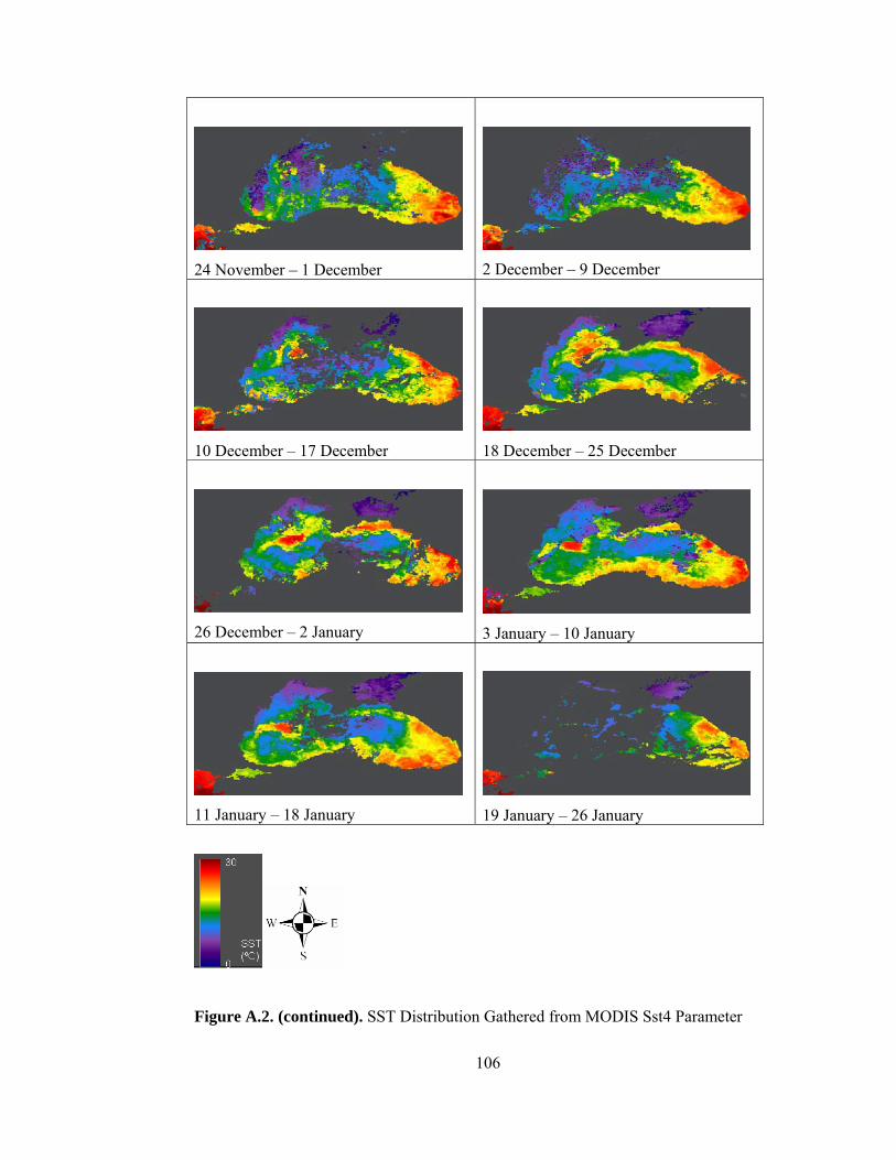
106
24 November – 1 December
2 December – 9 December
10 December – 17 December
18 December – 25 December
26 December – 2 January
3 January – 10 January
11 January – 18 January
19 January – 26 January
Figure A.2. (continued). SST Distribution Gathered from MODIS Sst4 Parameter

107
27 January – 3 February
4 February – 11 February
12 February – 19 February
20 February – 27 February
28 February – 7 March
8 March – 15 March
Figure A.2. (continued). SST Distribution Gathered from MODIS Sst4 Parameter in
Black Sea
Top Related