


Languages
Pages
Legal


Sensors 2008, 8, 4725-4741; DOI: 10.3390/s8084725
sensors ISSN 1424-8220
www.mdpi.org/sensors
Article
Detecting Land Subsidence in Shanghai by PS-Networking SAR Interferometry
Guoxiang Liu 1,*, Xiaojun Luo 1, Qiang Chen 1, Dingfa Huang 1 and Xiaoli Ding 2
1 Dept. of Surveying Engineering, Southwest Jiaotong University, Chengdu, China;
E-mails: [email protected] (Guoxiang Liu); [email protected] (Xiaojun Luo);
[email protected] (Qiang Chen); [email protected] (Dingfa Huang)
2 Dept. of Land Surveying and Geo-Informatics, The Hong Kong Polytechnic University, Hong Kong,
China; E-mail: [email protected] (Xiaoli Ding)
* Author to whom correspondence should be addressed.
Received: 14 July 2008; in revised form: 5 August 2008 / Accepted: 13 August 2008 / Published: 19 August 2008
Abstract: Existing studies have shown that satellite synthetic aperture radar (SAR)
interferometry has two apparent drawbacks, i.e., temporal decorrelation and atmospheric
contamination, in the application of deformation mapping. It is however possible to
improve deformation analysis by tracking some natural or man-made objects with steady
radar reflectivity, i.e., permanent scatterers (PS), in the frame of time series of SAR images
acquired over the same area. For detecting land subsidence in Shanghai, China, this paper
presents an attempt to explore an approach of PS-neighborhood networking SAR
interferometry. With use of 26 ERS-1/2 SAR images acquired 1992 through 2002 over
Shanghai, the analysis of subsiding process in time and space is performed on the basis of a
strong network which is formed by connecting neighboring PSs according to a distance
threshold. The linear and nonlinear subsidence, atmospheric effects as well as topographic
errors can be separated effectively in this way. The subsidence velocity field in 10 years
over Shanghai is also derived. It was found that the annual subsidence rates in the study
area range from -2.1 to -0.6 cm/yr, and the averaged subsidence rate reaches -1.1 cm/yr.
Keywords: permanent scatter, PS networking, radar interferometry, subsidence detection.
OPEN ACCESS

Sensors 2008, 8
4726
1. Introduction
As the largest metropolitan in China, Shanghai is directly close to the sea and Huangpu River. Built
on coastal sand and clay that lie 70 meters below the ground surface, this city has been suffering from
land subsidence for many years due to overuse of groundwater and rapid construction of
skyscrapers [1]. The historical record shows that the most severe subsidence occurred in the 1960s at a
rate of over 10 cm/yr - a rate that would have put the city below sea level by 1999 if it had not been
slowed down [1-2]. Since then the municipal government has taken some management actions such as
pumping water back into ground to mitigate the situation. However, the uneven subsidence at a rate of
1 cm/yr in recent years has still affected or deteriorated facilities such as subway tunnels, buildings,
roads, and water and sewage systems, thus resulting in huge economic loss [2].
Monitoring of land subsidence in Shanghai is apparently crucial for predicting potential geological
hazards and designing compensation strategies. Over the past decades, the subsidence data has been
collected on a regular basis by the conventional methods such as precise leveling and GPS [1-2] which
are time consuming, point-based and lack fine details. In recent years, we have focused on exploring a
new technique called differential interferometric synthetic aperture radar (DInSAR) to provide another
choice for efficiently detecting subsidence in Shanghai [3-4]. It is well known that DInSAR is viable
for regional deformation mapping with some prominent advantages such as high sensitivity to motion
and fine spatial resolution. Deformation extraction relies on comparison of phase values between SAR
images acquired at different time over the same area [5]. However, the full operational capability of
DInSAR in deformation monitoring has not been achieved yet. The major sources of uncertainty in
interferometric deformation measurements are temporal decorrelation and atmospheric influence [5-7].
To mitigate the aforementioned negative effects, Ferretti et al. developed a very generic technique
referred to as permanent-scatter (PS) technique to extract deformation information from the multiple
interferograms generated with a time series of SAR images [8]. Instead of full-resolution analysis, the
PS technique performs modeling and analyzing on PS targets, i.e., hard objects such as buildings, rocks,
bridges and dykes, which can maintain steady radar reflectivity even over months to years. On the basis
of the basic strategy of PS technique proposed by Ferretti et al. [8-9], this paper aims to improve both
accuracy and reliability for subsidence detection in Shanghai by considering spatial autocorrelation and
parameter adjustment. With the use of multiple interferograms, the analysis of subsiding process in
Shanghai is performed on a strong network which is formed by connecting neighboring PS points.
Such an approach is thereafter referred to as PS-networking SAR interferometry. Its algorithm
validation is conducted using 26 C-band SAR images acquired by the satellites ERS-1 and ERS-2 of
the European Space Agency (ESA) from 1992 to 2002 over Shanghai.
This paper is organized as follows. This part is followed by a brief description of data preprocessing
and PS-network formation. After this, we present the methodologies of data modeling and parameter
estimating. The testing results are then shown and discussed. Conclusions are given in the final section.

Sensors 2008, 8
4727
2. PS detection and PS-network formation
Unlike the conventional DInSAR only dealing with a single interferogram, the PS-networking SAR
interferometry utilizes the multiple interferograms to isolate deformation information from
atmospheric and topographic effects. Figure 1 shows the main procedures of PS-networking SAR
interferometry being used for estimating subsidence in Shanghai.
Figure 1. Flowchart of PS-networking SAR interferometry.
Given N+1 SAR images acquired at different time over the same area, they are first ranked by
imaging date order. One of them is then selected as the unique master image, while the remaining N
SAR images are used as the slave images, and thus resulting in N interferometric pairs
and N interferograms.
Calibrating and co-registering N+1 SAR images
Generating N differential
interferograms
Detecting PSs and forming PS-
network
Extracting time series of differential phases at PSs
PS-network modeling and linear subsidence estimation
Computing the residual phase increments
Estimating the residual phases at PSs
Deriving atmospheric effect by filtering
Deriving nonlinear subsidence by filtering

Sensors 2008, 8
4728
To guarantee the quality of all the interferograms, we select the optimal master image by
maximizing the joint correlation (JC) of all the images with [10]
∑=
⊥=N
kc
k,mDCc
mkc
mkm ffcTTcBBcN 1
,, ),(),(),(1γ (1)
where the function c is defined as
≥
<−=ax
axa
xaxc
0
||
1),( (2)
In equation (1), mγ denotes JC value when image m is used as the master; mkB ,⊥ , mkT , and k,m
DCf are the
spatial baseline (SB), the temporal baseline (TB) and the Doppler centroid difference (DCD) between
image k and m, respectively; index c means the coherence. In equation (2), a denotes the critical value
of SB, TB or DCD. We set the maximum SB, TB and DCD of all the interferograms as their respective
critical values. Let every image be the master and N+1 JC values can be obtained with a trial
computation by equation (1). The image corresponding to the maximum JC value is chosen as the
optimal master image.
Since the accurate co-registration of SAR imagery is a key prerequisite for any change detection, all
the SAR images have to be co-registered into the same space with sub-pixel accuracy [5]. N slave SAR
images are co-registered on sampling grids of the selected master image by maximizing correlation of
amplitude data between SAR acquisitions. As the subsequent PS detection is based on the statistical
calculation of SAR data, we calibrate all the SAR amplitude images in a similar way as Lyons &
Sandwell [11]. The unique radiometric calibration factor of each image is defined and calculated as a
ratio of the amplitude of each image (mean of all pixels) to the mean amplitude of the entire dataset.
Each SAR amplitude image is divided by this ratio to make the brightness between images consistent
and comparable.
In terms of PS detection, existing study shows that the statistical properties of phase data at any
time-coherent pixel can be analyzed by the time series of SAR amplitude data [9]. Although our PS
detection basically follows the strategy proposed by Ferretti et al. [9], we identify the PS candidates on
a pixel-by-pixel basis with use of all the co-registered and calibrated SAR amplitude images. First
derived are the overall mean A and the standard deviation (SD) Aσ of the entire amplitude dataset. At
each pixel the time series of the amplitude values is extracted to calculate the mean a and the SD aσ .
We label a pixel as a PS candidate if the following two criteria are satisfied simultaneously,
+≥
≤=
A
aa
Aa
.a
D
σ
σ
2
250 (3)
where aD is called amplitude dispersion index (ADI) [9]. By the second criteria, the false PSs are more
easily removed as the lower amplitude means less temporally coherent. We will eventually judge if the
PS candidates are true or false by PS networking based on phase data as discussed in the
next section.
After selection of all the PSs, we connect the neighboring PSs to form a network which is similar to
a conventional geodetic network like leveling or GPS network. It will be seen that such network can

Sensors 2008, 8
4729
provide a framework for modeling and improving parameter estimation and adjustment. Unlike a
triangular irregular network (TIN) as applied by Kampes & Adam [10] and Mora et al. [12], we freely
link the neighborhood PSs using a given threshold of Euclidian distance. Any two PSs l and p will be
connected only if the following criterion is met,
02222 )()(), ;,( SyyfxxfyxyxS lpalprppll ≤−⋅+−⋅= (4)
where (x , y ) are the pixel coordinates within the image space; rf and af are the scaling factors
(converting pixel dimension into geometric distances) in range and azimuth direction, respectively; 0S
is the distance threshold (e.g. 1 km) used to form a PS-PS connection which is thereafter called an arc.
It should be pointed out that 0S is generally chosen by mainly considering the atmospheric gradients
on the space domain. The faster the spatial variation of atmospheric delay, the shorter the distance
threshold. As an example, Figure 2 shows a network, herein termed freely-connected network (FCN),
constructed using inequality (4) with several PSs. It should be pointed out that such FCN is much
stronger than the TIN in terms of parameter estimation as presented in the next section.
Figure 2. An example of PS network.

Sensors 2008, 8
4730
3. Spatio-temporal modeling and estimating
3.1. Derivation and modeling of differential interferometric phase
Prior to modeling and estimating on the FCN, several procedures must be followed for data
reduction. These include computation of the initial interferograms and the differential interferograms.
Each initial interferogram can be derived by a pixel-wise conjugate multiplication (equivalent to phase
differencing) between the master SAR image and the co-registered slave SAR image. N initial
interferograms can be obtained in this way. In theory, a direct phase difference at each pixel is due to
several contributions, i.e., flat-earth trend, topography, ground motion, atmospheric delay and
decorrelation noise [5]. To highlight land subsidence, both the precise orbital data and the external
digital elevation model (DEM) can be utilized to remove the flat-earth trend and the topographic
effects from each initial interferogram, thus resulting in N differential interferograms. It should be
emphasized here that no spectral or phase filtering is performed during differential processing in order
to avoid deteriorating phase data at PS pixels.
Let us assume that the available DEM has errors and the land subsidence is of linear and nonlinear
accumulation in time. The differential interferometric phase at an arbitrary pixel with coordinates (x, y)
from the ith interferogram can be modeled as,
);,(cos),(4
),(sin
4);,( i
resiiiii TyxyxvTyxB
RTyx φθ
λπε
θλπ +⋅+⋅⋅
=Φ ⊥ (5)
where ⊥iB and iT are spatial and temporal baseline of the interferometric pair, respectively; λ , R and
θ are radar wavelength (5.66 cm for ERS), sensor-target distance, and radar incident angle,
respectively; ),( yxε , ),( yxv and );,( iresi Tyxφ are elevation error, subsidence velocity, and residual
phase, respectively. It should be noted that );,( ii TyxΦ is a wrapped phase value within the principal
interval of ) ,[ ππ− . Moreover, the residual phase );,( iresi Tyxφ can be viewed as the sum of several
components, including nonlinear subsidence nlsubiφ , atmospheric delay atm
iφ , and
decorrelation noise noiiφ .
3.2. PS-network modeling and linear subsidence estimation
In reality, any regionalized variable follows a fundamental geographic principal; that is the samples
that are spatially closer together tend to be more alike than those that are farther apart. The idea of
neighborhood differencing is therefore often employed to compensate some spatially correlated errors
or offsets. For example, the differential global positioning system (DGPS) may reduce some systematic
errors caused by atmospheric delay and orbital uncertainty so that the baseline components (coordinate
increments) between two adjacent stations can be determined more accurately. Likewise, the
differencing operation along each arc in PS network as shown in Figure 2 is helpful for improving
deformation analysis. For the ith interferogram, the differential interferometric phase increment along
an arc can be derived on the basis of equation (5), such that

Sensors 2008, 8
4731
) ; , ; ,(cos) , ; ,(4
) , ; ,(sin
4) ; , ; ,(
ippllresipplli
pplliipplli
TyxyxyxyxvT
yxyxBR
Tyxyx
φθλπ
εθλ
π
∆+⋅∆⋅⋅+
∆⋅⋅⋅⋅
≈∆Φ⊥
(6)
where ⊥iB , R and θ with the obvious symbol meaning are the averaged quantities of two PSs l and p,
i.e., 2/)( lipii BBB ⊥⊥⊥+= , 2/)( lp RRR += , lp θθθ += . ε∆ and v∆ are the increment of elevation
errors and the increment of linear displacement velocities, respectively. resiφ∆ is the increment of
residual phases, which can be extended as
) ; , ; ,() ; , ; ,(
) ; , ; ,() ; , ; ,(
ippllnoiiippll
atmi
ippllnlsubiippll
resi
TyxyxTyxyx
TyxyxTyxyx
φφ
φφ
∆+∆+
∆=∆ (7)
where nlsubiφ∆ , atm
iφ∆ and noiiφ∆ are the increment of nonlinear-subsidence phases, atmospheric phases,
and decorrelation noises, respectively.
It should be pointed out that the atmospheric effect and the nonlinear subsidence can most likely be
cancelled out by neighborhood differencing embodied in equation (6). It is now readily understandable
that we use a short distance thresholding when linking two PSs for networking. The modeling along arcs
facilitates the estimation of the two linear increments, i.e., ε∆ and v∆ , which are constant over time. The theoretical investigation by Ferretti et al. indicated that if res
iφ∆ is small enough, say
πφ <∆ resi , both ε∆ and v∆ can be indeed derived directly from the N wrapped interferograms [8]. In
fact, the solution of ε∆ and v∆ can be obtained by maximizing the following objective function [8-9]:
maximum)sin(cos1
1
=∆⋅+∆= ∑=
N
i
resi
resi j
Nφφγ (8)
where γ is called the arc’s model coherence (MC); 1−=j ; and resiφ∆ denotes the difference
between the measurement and the fitted value, such that
θλπε
θλπφ cos
4
sin
4 ⋅∆⋅⋅−∆⋅⋅⋅⋅
−∆Φ=∆⊥
vTBR
iiiresi (9)
Although the objective function is highly nonlinear and the phase datasets are measured in a
wrapped version, the two unknownsε∆ and v∆ of each arc can be determined by searching a pre-defined solution space (constraint) to maximize the MC value. In the case of perfect phase datasets γ
reaches the best value of 1, while in the case of total decorrelation γ reaches the worst value of 0. It
should be noted that the phase unwrapping can be avoided through the process of function optimization,
which is really a challenging task in data processing of the conventional DInSAR.
With equation (8) and (9) we can compute the increments of elevation errors and linear subsidence
velocities along all the arcs in the network. By trials with simulated data, we have found that the arcs have an accurate solution for ε∆ and v∆ if γ is not smaller than 0.45. The network is
therefore “cleaned up” by deleting some bad arcs and some isolated (false) PS candidates with such
MC thresholding. The reduced network can then be treated in a similar way as a leveling or GPS
network [13]. The least squares (LS) adjustment procedure is applied to eliminate the geometric

Sensors 2008, 8
4732
inconsistency in the network due primarily to uncertainty in phase data, and thus obtaining the most
probable values of the linear subsidence rates and elevation errors at PSs.
Taking the adjustment of a linear-subsidence network as an example, we present some mathematical
expressions as follows. A prototype observation equation for an arc is expressed as
Klplprvvv plpllp , ,2 ,1, , ,ˆˆ K=∀≠+∆=− (10)
where lv̂ and pv̂ denote the linear subsidence rate at PS p and l, respectively; plr is the correction
(residual) of plv∆ . K is the total number of all the true PSs. Suppose we have Q arcs in the network.
The matrix form of observation equations can hence be written as
111 ××××
+=⋅QQKKQRLXB (11)
where the coefficient matrix B is highly sparse and has the nonzero elements of either 1 or -1; L and R
are the vectors for the observations (increments) and the residuals, respectively, of all the arcs; X is the
vector for the unknown linear subsidence velocities to be estimated at all the true PSs, i.e.,
]ˆ ,, ˆ ,ˆ[ 21 KvvvX L= (12)
Furthermore, let the weighting matrix be
=
2
22
21
000
000
000
Q
P
γ
γγ
MMMM (3)
whose diagonal element is the square of MC value previously estimated for each arc. Therefore, the LS
solution of the unknowns X can be expressed as
PLBPBBX TT 1)( −= (14)
The above procedures can also be applied in a similar way onto the elevation-inconsistency network
to estimate the elevation errors at all the true PSs. The Kriging interpolator can be used to generate grid
data with the results available at sparse PSs [14]. As a remark, we underline that a reference point
without motion or elevation error should be selected according to a priori information to obtain a
unique solution with LS adjustment, and thus making all the estimates be related to the benchmark.
Moreover, it should be emphasized that the FCN used here is much stronger in terms of reliability than
the TIN. Our simulation study shows that the LS solution derived with the FCN is more accurate than
that derived with the TIN even though a small portion of measurements (ε∆ , v∆ ) are set as outliers
intentionally. This is because the redundancy number in the FCN is significantly larger than that
in the TIN.
3.3. Extraction of atmospheric effect and nonlinear subsidence
The further analysis focuses on isolating the nonlinear subsidence from the atmospheric delay. For
each interferometric pair, the residual phase increment (gradient) at each arc can be first calculated by
equation (9). The integration of gradients (i.e., phase unwrapping) of all the arcs in the network is then
performed by a weighted least squares method [15], and thus obtaining the residual phases at all the PS

Sensors 2008, 8
4733
pixels for each pair. As seen in equation (5), the residual phase is due to nonlinear subsidence,
atmospheric delay and decorrelation noise.
It is possible to separate the nonlinear subsidence from the undesired atmospheric delay because the
two terms have different spectral structure in space and time domain [8][12]. In terms of atmospheric
perturbation, a high correlation exists in space, but a significantly low correlation presents in time. In
terms of nonlinear subsidence, a strong correlation exists in space and a high correlation occurs in time.
It is however not easy to discriminate the spectral bands between the nonlinear subsidence and the
atmospheric effect if no a priori information is available. This implies that an exact separation of the
two terms is a challenging task. We basically follow a method by Ferretti et al. to isolate nonlinear
subsidence from atmospheric delay [8]. The atmospheric phase atm
MIφ of the master image (common to all the interferometric pairs) can be
estimated by
SpaceLP
N
i
resi
atmMI N _1
1
= ∑
=
φφ (15)
which means a low-pass (LP) filtering applied onto the mean of the sequence of residual phases. The atmospheric phase atm
iSI _φ of the ith slave image can then be derived by
{ }{ }SpaceLPTimeHP
resatmiSI ___ φφ = (16)
which means that a high-pass (HP) filtering is first applied onto the time series of residual phases and a LP filtering in space is then applied. The atmospheric phase atm
iφ of the ith differential interferogram is
thus obtained as the sum of atmMIφ and atm
iSI _φ . The nonlinear subsidence nlsubiS contained in the ith
interferometric pair is finally calculated by
( )atmi
resi
nlsubiS φφ
θπλ −=cos4
(17)
It should be noted that the decorrelation noise can be reduced by the operation of low-pass filtering in
space as shown in equation (15) and (16).
4. Dataset and subsidence result in Shanghai
To detect subsidence evolution in Shanghai metropolitan (China) by the procedures presented above,
we utilize 26 single look complex (SLC) SAR images which are available at hand. They were acquired
from 1992 to 2002 by two C-band (wavelength 6.5=λ cm) radar sensors onboard the satellites ERS-1
and ERS-2, respectively (both operated by European Space Agency). All the images were collected by
a nominal radar look angle of about 23º along the descending orbits. With a pixel size of 7.9 m in slant
range by 4.0 m in azimuth, each image covers the same area of about 100×100 km2 whose central
location is 121º28′E, 31º10′N. To optimize the interferometric combination, we determined the unique
master image by maximizing radar coherence of the entire dataset by equation (1). Eventually the SAR
image taken by ERS-2 on May 5, 1998 is chosen as the optimal master image. The remaining 25
images are used as the slave images, thus forming 25 interferometric pairs. Table 1 lists the parameters
of all the images, including spatial and temporal baseline with respect to the master image. For
detection of PSs, all the 26 amplitude images were calibrated by the procedures as briefed in section 2.

Sensors 2008, 8
4734
To generate interferograms, all the slave images were co-registered onto the sampling grids of the
master image.
Table 1. The parameters of 26 ERS-1/2 SAR images used in this study.
Note: the ⊥B and T are the normal baseline and the temporal baseline, respectively.
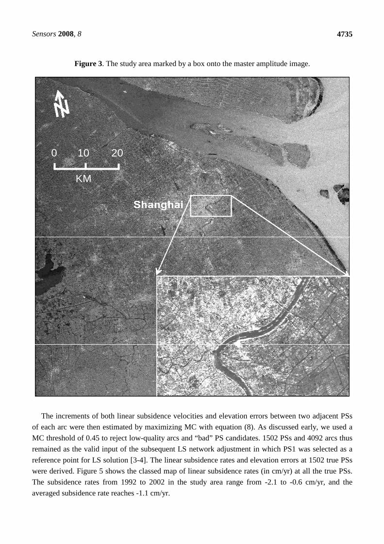
Existing studies indicate that the most serious subsidence in Shanghai has been taking place around
the downtown area, and reached a remarkable value of 2.63 m accumulated from 1921 to 1965 [1-2].
The further data reduction is therefore focused on the main downtown area of 7 km by 12 km. Figure 3
displays the study area of interest (AOI) marked by a box onto the master amplitude image, where the
inset shows the enlarged multi-image reflectivity map derived by averaging all the image patches of the
AOI. Its radiometric quality has been dramatically improved due to the reduction of speckle noises by
averaging. It is clearly visible that Huangpu River wriggles over the study area. The 25 differential
interferograms were generated by the “two-pass” method [4-5]. To remove both flat-earth and
topographic phases, we use the precise orbit state vectors (about 4-cm accuracy in the radial direction)
provided by Delft Institute for Earth-Oriented Space Research in Netherlands [8-10] and a DEM (about
5-m accuracy) which were generated using 1:50000 digital maps provided by State Bureau of
Surveying and Mapping, the national mapping agency of China.
The PS candidates were detected on a pixel-by-pixel basis by the statistical computation of time
series of amplitude values at each pixel. The pixel is determined as a PS candidate based on the criteria
of inequality (3). Figure 4 shows the distribution of all the 1520 PSs obtained in this way, which are
superimposed onto an optical orthoimage created with data from IKONOS sensor. In Figure 4, five PSs
marked by pentagram and PS1, PS2, …, PS5, respectively, will be used for later analysis of time series
of subsidence (see Figure 7). It can be noted that the high density of PSs (about 35/km2) appears in the
area with dense buildings, while the PSs are rare in some farmlands due to serious temporal
decorrelation. We formed a very strong network by freely connecting each PS and all the others if their
distance is less than 1 km, as defined in inequality (4), resulting in 4202 arcs.
No. Platform
-orbit Imaging
Date
⊥B (m)
T (day)
No. Platform
-orbit Imaging
Date ⊥B (m)
T (day)
1 2 3 4 5 6 7 8 9 10 11 12 13
E1-04657 E1-06160 E1-09166 E1-10669 E1-12172 E1-19530 E1-22035 E1-24039 E1-24540 E2-04867 E1-25542 E2-05869 E2-13384
1992.06.06 1992.09.19 1993.04.17 1993.07.31 1993.11.13 1995.04.10 1995.10.02 1996.02.19 1996.03.25 1996.03.26 1996.06.03 1996.06.04 1997.11.11
504 146 -36 274 -639 -207 178 505
-1144 -1000 -1253 -1104 -762
-2159 -2054 -1844 -1739 -1634 -1121 -946 -806 -771 -770 -701 -700 -175
14 15 16 17 18 19 20 21 22 23 24 25 26
E2-14887 E2-15388 E2-15889 E2-20899 E2-23905 E2-24406 E2-26410 E2-26911 E2-28414 E2-34426 E2-37432 E2-37933 E2-38434
1998.02.24 1998.03.31 1998.05.05 1999.04.20 1999.11.16 1999.12.21 2000.05.09 2000.06.13 2000.09.26 2001.11.20 2002.06.18 2002.07.23 2002.08.27
-1239 -487
0 247 -348 -141 303 -158 290 -198 1048 144
-1021
-70 -35 0
350 560 595 735 770 875 1295 1505 1540 1575
Sensors 2008, 8
4735
Figure 3. The study area marked by a box onto the master amplitude image.
10 20 0
KM
The increments of both linear subsidence velocities and elevation errors between two adjacent PSs
of each arc were then estimated by maximizing MC with equation (8). As discussed early, we used a
MC threshold of 0.45 to reject low-quality arcs and “bad” PS candidates. 1502 PSs and 4092 arcs thus
remained as the valid input of the subsequent LS network adjustment in which PS1 was selected as a
reference point for LS solution [3-4]. The linear subsidence rates and elevation errors at 1502 true PSs
were derived. Figure 5 shows the classed map of linear subsidence rates (in cm/yr) at all the true PSs.
The subsidence rates from 1992 to 2002 in the study area range from -2.1 to -0.6 cm/yr, and the
averaged subsidence rate reaches -1.1 cm/yr.

Sensors 2008, 8
4736
Figure 4. All the detected PSs superimposed onto an optical orthoimage.
PS1
PS2
PS3
PS4
PS5
121.46 121.48 121.5 121.52 121.54 121.56 121.58
Longitude (Deg.)
31.22
31.24
31.26
31.28
Lat
itude
(D
eg.)
Figure 5. The classed map of linear subsidence rates at all the PSs.
-0.6~-0.9
-0.9~-1.2
-1.2~-1.5
-1.5~-1.8
-1.8~-2.1
Unit: cm/yr
121.46 121.48 121.5 121.52 121.54 121.56 121.58
Longitude (Deg.)
31.22
31.24
31.26
31.28
Lat
itud
e (D
eg.)
It should be pointed out that the FCN used in our approach is more advantageous than TIN used
elsewhere in terms of accuracy and reliability for estimating subsidence rates and elevation errors at
PSs, although the former incurs much heavier computation burden than the latter. The reliability with
FCN is significantly enhanced because it has much more connections (arcs) between adjacent PSs than
TIN. In other words, the total number of redundant observations in FCN is much larger than that in
TIN. Hence the LS estimator for FCN is less disturbed by outliers. Our testing results derived with
simulated data indicated that the FCN-based LS estimation can efficiently resist against a small portion

Sensors 2008, 8
4737
of outliers in measurements (ε∆ , v∆ ). In addition, the FCN tends to remain more PS points than TIN
when deleting some “bad” arcs by MC thresholding. The weaker links in TIN may cause more isolated
PSs which can not be connected with other PSs, and some true PSs are erroneously rejected. The
stronger links in FCN are therefore useful for recovering the finer details of deformation field.
Figure 6. The atmospheric phases in the partial AOI for the master image.
Longitude (Deg.)
Lat
itud
e (D
eg.)
121.46 121.48 121.5 121.52 121.54 121.56 121.58
31.22
31.23
31.24
31.25
31.26
31.27
31.28
-1 -0.8 -0.6 -0.4 -0.2 0 0.2rad
The atmospheric delay and nonlinear subsidence in the study area were finally separated by a time-
space filtering method as discussed in section 3.3. Prior to such separation, the residual phases in each
differential interferogram were extracted by detrending both linear subsidence and topographic effect.
The atmospheric phases of the master image (by ERS-2 on May 5, 1998) were derived by a LP space
filtering applied onto the mean of 25 residual-phase images (see equation (15)), while the atmospheric
phases of any slave image were estimated by time-space filtering according to equation (16). As an
example, Figure 6 shows the atmospheric phases in the partial AOI for the master image, which vary
from -1.2 to 0.4 radians, i.e., range change of -5 to 2 mm in radar line of sight. As a remark, we stress
that exactly separating nonlinear subsidence from atmospheric artifacts is indeed a challenging task.
The further improvement on this point is still required, particularly by integrating a priori information
on atmosphere and subsidence available from some other monitoring approaches such as GPS
permanent tracking network.

Sensors 2008, 8
4738
Figure 7. Time series of subsidence at 5 PSs as marked in Figure 4.
1992 1993 1994 1995 1996 1997 1998 1999 2000 2001 2002 2003-15
-10
-5
0
Time (year)
Su
bsi
den
ce (
cm)
PS1PS2PS3PS4PS5
Figure 8. Perspective view of the subsidence field accumulated between June 1992 and
August 2002.
After deriving atmospheric phases, equation (17) was used to calculate nonlinear subsidence. The
time series of subsidence was eventually obtained as a sum of linear and nonlinear parts. As examples,
Figure 7 shows the so-obtained temporal evolution of subsidence at 5 PSs (see Figure 4) in the central

Sensors 2008, 8
4739
part of the study area, where about 15-cm land sinking was accumulated from 1992 to 2002. It is
obvious that the linear subsidence trend dominates the nonlinear component with a peak-to-trough
variation of about 4 cm in this study area. For visualization, a perspective view of the entire subsidence
field is shown in Figure 8, where the remarkable sinking parts can be better appreciated. Maximum and
minimum subsidence values are -18 and -9 cm, respectively.
In recent years, both precise leveling and GPS survey have been carried out to monitor subsidence
in Shanghai by some authorities [1-2]. Both the first- and second-order leveling are carried out once
per year for benchmarks in the downtown area. The annual subsidence rates (see Figure 5) and the
accumulated quantity (see Figure 8) estimated with PS-networking SAR interferometry are in good
agreement with the leveling subsidence results reported in some open literature [1-2]. This indicates
that our approach presented in this study is effective for detecting land subsidence in Shanghai. The
current land sinking is highly related to the large-scale urban construction and the overuse of
groundwater. Especially from 1992 to 1995, the skyscrapers’ constructions are most remarkable [1]. It
should be noted that the estimated vertical displacement may also contain the settlement of skyscrapers,
and not purely the natural subsidence of the land surface. The annual subsidence rate is however much
smaller than that occurring in the 1980’s. This is primarily attributed to some mitigation strategies
proposed by city managers and planners, which include reducing groundwater withdrawal, increasing
river water use, pumping water back into depleted aquifers, and utilizing light materials for
construction.
5. Conclusions
To mitigate the negative impacts of both temporal decorrelation and atmospheric delay on mapping
deformation with conventional DInSAR, this paper has presented an approach called PS-networking
SAR interferometry for detection of land subsidence in Shanghai, China. With use of 26 ERS-1/2 SAR
images acquired 1992 through 2002 over Shanghai, the time series of land subsidence is analyzed with
a very strong network which is formed by freely connecting neighboring PSs according to a given
distance threshold. The mathematical models and computing methods are addressed systematically by
considering spatial autocorrelation and LS parameter estimation. The linear and nonlinear subsidence,
atmospheric effect as well as topographic error were separated effectively in this way. The subsidence
velocity field in 10 years over Shanghai was also derived. It was found that the annual subsidence rates
in the study area range from -2.1 to -0.6 cm/yr, and the averaged subsidence rate reaches -1.1 cm/yr.
The maximum subsidence accumulated in 10 years is up to -18 cm. These are generally in good
agreement with the leveling subsidence results reported elsewhere. In addition, the testing results
indicated that the FCN proposed in this study is more advantageous than the TIN used elsewhere in
terms of reliability for estimating subsidence rates and elevation errors at PSs, although the former
incurs much heavier computation burden than the latter.
With further improvement, it is anticipated that PS-networking SAR interferometry would become
an operational tool to monitor the slowly-accumulated urban subsidence, and thus complementing the
conventional geodetic tools such as GPS and leveling. In China, there are a number of cities which are
suffering from land subsidence. Besides Shanghai, the other typical sinking cities include Tianjin and

Sensors 2008, 8
4740
Taiyuan. The reliable and prompt measurements reflecting land subsidence evolution are valuable for
assessing and mitigating some geological hazards related to land sinking.
Acknowledgements
The work presented here was partially supported by three grants from the National Natural Science
Foundation of China (Project No. 40774004, 40374003, 40474008) and ESA Category-1 Data Use
Program. The authors would like to thank State Bureau of Surveying and Mapping in China and the
Delft University of Technology for providing topographic maps and precise orbital data, respectively.
In addition, the authors are also very thankful to two anonymous reviewers for their
valuable comments.
References and Notes
1. Liu, Y.; Zhang, X.L.; Wan, G.F.; Han, Q.D. The situation of land subsidence within Shanghai in
recent years and its countermeasure. Chin. J. Geol. Hazard Control 1998, 9 (2), 13-17.
2. Liu, Y. Preventive measures for land subsidence in Shanghai and their effects. Volcanology &
Mineral Resources 2000, 21 (2), 107-111.
3. Chen, Q.; Liu, G.X., Li, Y.Q.; Ding, X.L. Automated detection of permanent scatterers in radar
interferometry: algorithm and testing results. Acta Geodaetica et Cartographica Sinica 2006, 35
(2), 112-117.
4. Liu, G.X.; Chen, Q. Detecting ground deformation with permanent-scatterer network in radar
interferometry: algorithm and testing result. Acta Geodaetica et Cartographica Sinica 2007, 36
(1), 13-18.
5. Liu, G.X. In Monitoring of Ground Deformations with Radar Interferometry; Publishing House of
Surveying and Mapping: Beijing, 2006; pp 1-148.
6. Zebker, H.A.; Villaseno, J. Decorrelation in interferometric radar echoes. IEEE Transactions on
Geoscience and Remote Sensing 1992, 30 (5), 950-959.
7. Zebker, H.A.; Rosen, P.A.; Hensley, S. Atmospheric effects in interferometric synthetic aperture
radar surface deformation and topographic maps. J. Geophysical Res. 1997, 102 (B4), 7547-7563.
8. Ferretti, A.; Prati, C.; Rocca, F. Nonlinear subsidence rate estimation using permanent scatterers
in differential SAR interferometry. IEEE Transactions on Geoscience and Remote Sensing 2000,
38 (5), 2202-2212.
9. Ferretti, A.; Prati, C.; Rocca, F. Permanent scatterers in SAR interferometry. IEEE Transactions
on Geoscience and Remote Sensing 2001, 39 (1), 8-20.
10. Kampes, B.M.; Adam, N. Velocity field retrieval from long term coherent points in radar
interferometric stacks. In Proceedings of IGARSS, Toulouse, 2003; pp941-943.
11. Lyons, S.; Sandwell, D. Fault creep along the southern San Andreas from InSAR, permanent
scatterers, and stacking. J. Geophysical Res. 2003, 108 (B1), 2047-2070.
12. Mora, O.; Mallorqui, J.J.; Broquetas, A. Linear and nonlinear terrain deformation maps from a
reduced set of interferometric SAR images. IEEE Transactions on Geoscience and Remote
Sensing 2003, 41 (10), 2243-2253.

Sensors 2008, 8
4741
13. Wolf, P.R.; Ghilani, C.D. In Adjustment Computations: Statistics and Least Squares in Surveying
and GIS. John Wiley & Sons, Inc: New York, 1997; pp 10-150.
14. Olea, R.A. In Geostatistics for Engineers and Earth Scientists; Kluwer Academic Publishers:
Dordrecht, The Netherlands, 1999; pp 20-105.
15. Ghiglia, D.C.; Pritt, M.D. In Two-Dimensional Phase Unwrapping: Theory, Algorithms, and
Software; John Wiley & Sons, Inc: New York, 1998; pp 200-325.
© 2008 by the authors; licensee Molecular Diversity Preservation International, Basel, Switzerland.
This article is an open-access article distributed under the terms and conditions of the Creative
Commons Attribution license (http://creativecommons.org/licenses/by/3.0/).
Top Related