


Languages
Pages
Legal


Design of a Non-Contact Vibration Measurement and AnalysisSystem for Electronic Board Testing
ByKrissa Elizabeth Arn
B.S. Engineering MechanicsUnited States Air Force Academy, 2002
SUBMITTED TO THE DEPARTMENT OF MECHANICAL ENGINEERING INPARTIAL FULFILLMENT OF THE REQUIREMENTS FOR THE DEGREE OF
MASTER OF SCIENCE IN MECHANICAL ENGINEERINGAT THE
MASSACHUSETTS INSTITUTE OF TECHNOLOGY
JUNE 2004
� 2004 Krissa Elizabeth Arn. All rights reserved
The author hereby grants to MIT permission to reproduce and to distribute publicly paperand electronic copies of this thesis document in whole or in part.
Signature ofAuthor:________________________________________________________
Department of Mechanical EngineeringMay 2004
Certified by:_______________________________________________________________George Costa
Charles Stark Draper LaboratoryThesis Supervisor
Certified by:_______________________________________________________________Warren P. Seering
Weber-Shaughness Professor of Mechanical EngineeringThesis Advisor
Accepted by:______________________________________________________________Ain A. Sonin
Chairman, Committee on Graduate StudiesDepartment of Mechanical Engineering

Report Documentation Page Form ApprovedOMB No. 0704-0188
Public reporting burden for the collection of information is estimated to average 1 hour per response, including the time for reviewing instructions, searching existing data sources, gathering andmaintaining the data needed, and completing and reviewing the collection of information. Send comments regarding this burden estimate or any other aspect of this collection of information,including suggestions for reducing this burden, to Washington Headquarters Services, Directorate for Information Operations and Reports, 1215 Jefferson Davis Highway, Suite 1204, ArlingtonVA 22202-4302. Respondents should be aware that notwithstanding any other provision of law, no person shall be subject to a penalty for failing to comply with a collection of information if itdoes not display a currently valid OMB control number.
1. REPORT DATE 16 JUL 2004
2. REPORT TYPE N/A
3. DATES COVERED -
4. TITLE AND SUBTITLE Design of a Non-Contact Vibration Measurement and Analysis Systemfor Electronic Board Testing
5a. CONTRACT NUMBER
5b. GRANT NUMBER
5c. PROGRAM ELEMENT NUMBER
6. AUTHOR(S) 5d. PROJECT NUMBER
5e. TASK NUMBER
5f. WORK UNIT NUMBER
7. PERFORMING ORGANIZATION NAME(S) AND ADDRESS(ES) Massachusetts Institute of Technology
8. PERFORMING ORGANIZATIONREPORT NUMBER
9. SPONSORING/MONITORING AGENCY NAME(S) AND ADDRESS(ES) 10. SPONSOR/MONITOR’S ACRONYM(S)
11. SPONSOR/MONITOR’S REPORT NUMBER(S)
12. DISTRIBUTION/AVAILABILITY STATEMENT Approved for public release, distribution unlimited
13. SUPPLEMENTARY NOTES See also ADM001678, MIT-CI04-428, The original document contains color images.
14. ABSTRACT
15. SUBJECT TERMS
16. SECURITY CLASSIFICATION OF: 17. LIMITATION OF ABSTRACT
UU
18. NUMBEROF PAGES
136
19a. NAME OFRESPONSIBLE PERSON
a. REPORT unclassified
b. ABSTRACT unclassified
c. THIS PAGE unclassified
Standard Form 298 (Rev. 8-98) Prescribed by ANSI Std Z39-18

2
[THIS PAGE INTENTIONALLY LEFT BLANK]

3
Design of a Non Contact Vibration Measurement and AnalysisSystem for Electronic Board Testing
byKrissa Elizabeth Arn
Submitted to the Department of Mechanical Engineering onMay 7, 2004, in partial fulfillment of the requirements for the
Degree of Master of Science in Mechanical Engineering.
Abstract
Traditional vibration measurement methods involve placing accelerometers atdiscrete locations on a test object. In cases where the test specimen is small in mass, theaddition of these measurement transducers can alter its dynamic behavior and lead toerroneous test data. In this thesis a Non-Contact Vibration Measurement and AnalysisSystem has been designed, built, and tested for electronic board testing. Through a productdesign process, all feasible methods were considered and three optically based conceptswere explored: holographic interferometry, area scaling, and displacement sensor grid.Through concept testing and analysis, the displacement sensor grid method was chosen forthe design.
The final system incorporates four laser displacement sensors with a verticalscrolling mechanism that attaches to the vibration table’s side rails. This manual scanningsystem provides a quick, low cost method for capturing multiple points on the test objectduring vibration testing. The MATLAB based software package acquires the raw sensoroutput and processes it with a five step analysis program. With this software, an 8x4 gridof electronic board displacements were easily transformed into a movie showing the boarddisplacing through its first mode. The system requires the sensors be positioned 1cm awayfrom the test object with the sensors reading up to ±1mm of movement. The sensors havea maximum sample rate of 7.8 kHz and can be used to measure the displacements of anysurface type or material. The measurement grid resolution is 0.7 inches horizontally and0.4 inches vertically. Testing showed that the system captured the natural frequency andpeak displacement of the board’s first mode within 1.5% accuracy and 0.7% accuracyrespectively when compared with previous accelerometer grid testing.
Exceeding its design goals, this non-contact measurement and analysis deviceprovides a highly versatile, accurate, and low cost optical alternative to accelerometers.Also it shows numerous benefits over more complex and costly optical measurementmethods. The use of this system eliminates any question of whether mass loading effectsare tainting vibration test data. A hardware and software manual are included for referenceat the end of this thesis along with a software CD.
Technical Supervisor: George CostaTitle: Technical Staff, Charles Stark Draper Laboratory
Thesis Advisor: Warren P. SeeringTitle: Weber-Shaughness Professor of Mechanical Engineering

4
[THIS PAGE INTENTIONALLY LEFT BLANK]

5
Acknowledgements
I would like to convey my sincere gratitude to all of the people who have helpedme with my master’s work.
First, I would like to thank the Air Force and Draper Laboratory for the opportunityto complete my master’s degree at MIT. As a graduate student, Draper providesexceptional resources, material assistance, expert personnel, and support. I would like tothank all of GBB2 and more specifically, thanks to Sonia Gulbankian and Dave Black foralways knowing the answers to my questions or finding them out. Thanks to EdMcCormack in the machine shop for helping make my drawings a reality. Thanks to LarryFallon and all the guys in the Environmental Test Facility for operating the vibration tablefor my testing. And I cannot forget Linda Holland - thanks for moving me into a windowoffice.
I would like to thank Professor Warren Seering, my MIT advisor, for taking timeout of his busy schedule to provide valuable feedback and suggestions.
George Costa, my Draper Supervisor, deserves my greatest thanks. He not onlyguided my thesis work, he ensured there was always funding for my project, wasconstantly available to help me diagnose problems at a minutes notice, and provided theessential insight and expertise to make my thesis a success. Thanks!
A special shout out to my roommates, Bethany and Susan. You have made mytime in Apt 7C a constant blast. Thanks for your friendship and company. I am trulyappreciative to Ron and Carol Stott for opening their house to me, doing my laundry, andmaking Bethany and I dinner after our numerous late night rock climbing adventures. Tomy Draper Officemate, Carissa, and my MIT friend, Michelle, it was a pleasure to get toknow the two of you. I hope you know that you are always welcome wherever the AirForce takes me.
I would like to thank my family for helping me fulfill my life long dream ofattending MIT. Thanks for your love and support.
Finally, I want to thank my husband, Kevin Watry, for listening, support, sacrifice,and words of encouragement. It has been a long two years apart - I look for to our futuretogether.
This thesis was prepared at The Charles Stark Draper Laboratory, Inc., under ContractN00030-04-C-0010, sponsored by the Department of the Navy Strategic SystemsPrograms.
Publication of this thesis does not constitute approval by Draper or the sponsoring agencyof the findings or conclusions contained herein. It is published for the exchange andstimulation of ideas.
The views expressed in this thesis are those of the author and do not reflect the officialpolicy or position of the United States Air Force, Department of Defense, or the U.S.Government.
___________________________________________

6
Krissa E. Arn, 2 LT, USAF 7 May 2004
Assignment
Draper Laboratory Report Number T-1487
In consideration for the research opportunity and permission to prepare my thesis by and atThe Charles Stark Draper Laboratory, Inc., I hereby assign my copyright of the thesis toThe Charles Stark Draper Laboratory, Inc., Cambridge, Massachusetts.
___________________________________________Krissa E. Arn, 2 LT, USAF 7 May 2003
7
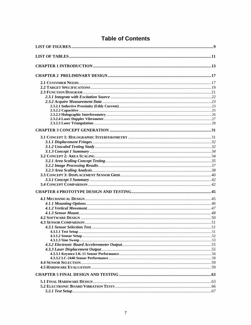
Table of ContentsLIST OF FIGURES .........................................................................................................................................9
LIST OF TABLES .........................................................................................................................................11
CHAPTER 1 INTRODUCTION ..................................................................................................................13
CHAPTER 2 PRELIMINARY DESIGN....................................................................................................17
2.1 CUSTOMER NEEDS................................................................................................................................172.2 TARGET SPECIFICATIONS ....................................................................................................................192.3 FUNCTION DIAGRAM ............................................................................................................................21
2.3.1 Integrate with Excitation Source .................................................................................................222.3.2 Acquire Measurement Data .........................................................................................................23
2.3.2.1 Inductive Proximity (Eddy Current)...................................................................................................232.3.2.2 Capacitive ..............................................................................................................................................252.3.2.3 Holographic Interferometry.................................................................................................................262.3.2.4 Laser Doppler Vibrometer ...................................................................................................................272.3.2.5 Laser Triangulation ..............................................................................................................................28
CHAPTER 3 CONCEPT GENERATION ..................................................................................................31
3.1 CONCEPT 1: HOLOGRAPHIC INTERFEROMETRY ................................................................................313.1.1 Displacement Fringes...................................................................................................................323.1.2 Unscaled Testing Study ................................................................................................................323.1.3 Concept 1 Summary .....................................................................................................................34
3.2 CONCEPT 2: AREA SCALING ................................................................................................................343.2.1 Area Scaling Concept Testing ......................................................................................................353.2.2 Image Processing Results.............................................................................................................373.2.3 Area Scaling Analysis...................................................................................................................38
3.3 CONCEPT 3: DISPLACEMENT SENSOR GRID........................................................................................403.3.1 Concept 3 Summary .....................................................................................................................42
3.4 CONCEPT COMPARISON .......................................................................................................................42
CHAPTER 4 PROTOTYPE DESIGN AND TESTING.............................................................................45
4.1 MECHANICAL DESIGN..........................................................................................................................454.1.1 Mounting Options.........................................................................................................................464.1.2 Vertical Movement........................................................................................................................474.1.3 Sensor Mount................................................................................................................................48
4.2 SOFTWARE DESIGN ..............................................................................................................................504.3 SENSOR COMPARISON ..........................................................................................................................51
4.3.1 Sensor Selection Test....................................................................................................................514.3.1.1 Test Setup ..............................................................................................................................................514.3.1.2 Sensor Setup ..........................................................................................................................................524.3.1.3 Sine Sweep .............................................................................................................................................53
4.3.2 Electronic Board Accelerometer Output......................................................................................554.3.3 Laser Displacement Output..........................................................................................................55
4.3.3.1 Keyence LK-11 Sensor Performance...................................................................................................564.3.3.2 LC-2440 Sensor Performance ..............................................................................................................58
4.4 SENSOR SELECTION..............................................................................................................................594.5 HARDWARE EVALUATION ....................................................................................................................59
CHAPTER 5 FINAL DESIGN AND TESTING .........................................................................................63
5.1 FINAL HARDWARE DESIGN ..................................................................................................................635.2 ELECTRONIC BOARD VIBRATION TESTS .............................................................................................66
5.2.1 Test Setup......................................................................................................................................67

8
5.2.2 Test Procedures ............................................................................................................................695.2.2.1 Vibration Table Configuration ............................................................................................................715.2.2.2 Expected Software Output ...................................................................................................................71
5.2.3 Test Results and Analysis Methods ..............................................................................................725.2.3.1 Analysis Step One: Capture First Mode .............................................................................................735.2.3.2 Analysis Step Two: De-noise Data .......................................................................................................75
5.2.3.2.1 Band Pass Filter..............................................................................................................................775.2.3.2.2 Wavelet De-Noising .......................................................................................................................795.2.3.2.3 Method Comparison: Filtering vs. Wavelet De-Noising.................................................................82
5.2.3.3 Analysis Step Three: Find Frequencies...............................................................................................835.2.3.3.1 Zero Crossing Algorithm................................................................................................................835.2.3.3.2 Interpolation and Averaging ...........................................................................................................845.2.3.3.3 Find Frequencies ............................................................................................................................845.2.3.3.4 Find Frequency Results: Original vs. De-noised ............................................................................86
5.2.3.4 Analysis Step Four: Clean Modal Data...............................................................................................865.2.3.5 Analysis Step Five: Create Movie ........................................................................................................88
CHAPTER 6 SYSTEM PERFORMANCE .................................................................................................93
6.1 ACCELEROMETER GRID COMPARISON ...............................................................................................936.2 CENTER ACCELEROMETER COMPARISON ..........................................................................................976.3 LASER VERSUS ACCELEROMETER DISCUSSION..................................................................................986.4 HARDWARE VIBRATION .......................................................................................................................986.5 SYSTEM SPECIFICATIONS...................................................................................................................100
CHAPTER 7 CONCLUSIONS AND RECOMMENDATIONS..............................................................103
7.1 CONCLUSIONS.....................................................................................................................................1047.2 RECOMMENDATIONS ..........................................................................................................................105
REFERENCES.............................................................................................................................................107
HARDWARE MANUAL ............................................................................................................................109
SOFTWARE MANUAL..............................................................................................................................121

9
List of Figures
Figure 1-1 Basic Piezoelectric Accelerometer [1] ...............................................................14Figure 2-1 Function Diagram...............................................................................................21Figure 2-2 Vibration Shaker Table Shown in Horizontal Motion Position .........................22Figure 2-3 Board Excitation Source: TA 165 Electro Dynamic Slip Table ........................22Figure 2-4 Keyence Inductive Proximity Sensors [5]..........................................................24Figure 2-5 Capacitive Sensor [6] .........................................................................................25Figure 2-6 Holographic Interfermetric Setup.......................................................................26Figure 2-7 Laser Triangulation Sensor [5]...........................................................................28Figure 2-8 Area Scaling Technique Variables .....................................................................29Figure 3-1 Interference Fringe Example [8] ........................................................................32Figure 3-2 Fringe Contours on Pixel Grid ...........................................................................33Figure 3-3 Electronic Board with Discrete Area Label .......................................................35Figure 3-4 Top View of Testing Diagram............................................................................36Figure 3-5 Testing Field of View.........................................................................................36Figure 3-6 Area Scaling Concept Tests Completed.............................................................37Figure 3-7 Test Parameters ..................................................................................................38Figure 3-8 Minimum Detectable Dot Growth......................................................................39Figure 3-9 Displacement Sensor Grid Example...................................................................41Figure 4-1 Shaker Table Sketch...........................................................................................46Figure 4-2 Shaker Table Mounting Scheme: Drill Press Vise.............................................47Figure 4-3 Discrete Vertical Movement: Holes ...................................................................47Figure 4-4 Vertical Movement: Slot ....................................................................................48Figure 4-5 Sensor Mount in Both Sensor Configurations....................................................49Figure 4-6 Sensor Selection Hardware Design ....................................................................50Figure 4-7 Sensor Selection Hardware Design with Vises ..................................................50Figure 4-8 Data Acquisition MATLAB Program: Laser Vibe Test 1.0 ..............................50Figure 4-9 Electronic Board Test Setup...............................................................................51Figure 4-10 Hardware Test Setup ........................................................................................52Figure 4-11 Displacement Sensor Setup Diagram...............................................................53Figure 4-12 Vibe Table Sine Sweep Representation ...........................................................54Figure 4-13 Vibration Table Sine Sweep Displacement vs. Frequency ..............................54Figure 4-14 Typical Accelerometer Output for Electronic Board .......................................55Figure 4-15 Center of the Board LK-11 Sensor Output.......................................................56Figure 4-16 Low Frequency LK-11 Test Data Comparison with Vibration Table
Displacement................................................................................................................56Figure 4-17 Comparison of Vibration Table and Board Displacement in the First Mode
Region ..........................................................................................................................57Figure 4-18 LK-11 Sensor Test Noise .................................................................................58Figure 4-19 Center of the Board LC-2440 Sensor Output...................................................58Figure 4-20 LC-2440 Sensor Output: First Mode Region ...................................................59Figure 4-21 Hardware Accelerometer Location ..................................................................60Figure 4-22 Comparison of Sensor Head Displacement with Center of the Board
Displacement................................................................................................................61

10
Figure 5-1 Final Hardware Setup.........................................................................................64Figure 5-2 Discrete Vertical Movement Mechanism...........................................................65Figure 5-3 One Centimeter Vertical Movement Resolution Diagram.................................65Figure 5-4 Sensor Mount .....................................................................................................66Figure 5-5 Electronic Board Displacement Grid Diagram ..................................................67Figure 5-6 Test Setup ...........................................................................................................67Figure 5-7 Sensor Wiring Diagram......................................................................................68Figure 5-8 Accelerometer Locations on Test Setup.............................................................68Figure 5-9 Assembly of Laser Vibration System on Vibration Table .................................69Figure 5-10 Laser Vibration Test 2.0: AcquireData.m ........................................................71Figure 5-11 Typical Vibration Sensor Output .....................................................................72Figure 5-12 Typical Unbiased Displacement vs Time Sensor Output.................................73Figure 5-13 Typical Sensor Output Zoomed In ...................................................................74Figure 5-14 First Mode Region............................................................................................74Figure 5-15 Step One Analysis GUI: Capture First Mode...................................................75Figure 5-16 First Mode Region Power Spectral Density Plot: FFT.....................................77Figure 5-17 Bandpass Filter Design.....................................................................................78Figure 5-18 PSD of Filtered Sensor Data ............................................................................78Figure 5-19 Original vs Filtered Sensor Data ......................................................................79Figure 5-20 DMEY Wavelet Decomposition of Modal Region ..........................................80Figure 5-21 Original vs De-Noised Sensor Data .................................................................81Figure 5-22 PSD of De-Noised Data ...................................................................................81Figure 5-23 Original, Filtered, and Denoised Comparison..................................................82Figure 5-24 Step Two Analysis GUI: De-noise...................................................................82Figure 5-25 Zero Crossing Algorithm Results.....................................................................83Figure 5-26 Zero Crossings with Linear Interpolation of Data............................................84Figure 5-27 Find Frequency Algorithm Results ..................................................................85Figure 5-28 Step Three Analysis GUI: Find Frequencies of Mode .....................................85Figure 5-29 Find Frequency Algorithm Results: Original vs. De-noised Data ...................86Figure 5-30 Original vs. Cleaned Modal Displacement.......................................................87Figure 5-31 Polynomial Fit of Cleaned Modal Displacement .............................................87Figure 5-32 Step Four Analysis GUI: Clean Modal Data....................................................88Figure 5-33 Step Five Analysis GUI: Create First Mode Movie .........................................89Figure 5-34 Test One First Mode Results ............................................................................90Figure 5-35 Test Two First Mode Results ...........................................................................90Figure 5-36 Laser Grid Results: Maximum Displacement ..................................................91Figure 6-1 Overall Accelerometer Grid Locations on Electronic Board .............................94Figure 6-2 Individual Accel Grid Location and 1st Natural Frequencies.............................94Figure 6-3 Accel Grid 3-D Output: Acceleration and Displacement at First Natural
Frequency.....................................................................................................................95Figure 6-4 Accel Grid: Maximum Displacement of Electronic Board During Sine Sweep96Figure 6-5 First Mode Max Displacement Comparison: Laser versus Accelerometer Output
......................................................................................................................................97Figure 6-6 Hardware Accelerometer Location ....................................................................99Figure 6-7 Magnitude of Hardware Vibration .....................................................................99

11
List of Tables
Table 2-1 Customer Needs and Their Relative Importance.................................................18Table 2-2 Needs-Metric Table .............................................................................................19Table 2-3 Target Specifications ...........................................................................................19Table 3-1 Displacement Grid Sensor Comparison...............................................................42Table 3-2 Concept Comparison Matrix................................................................................43Table 6-1 First Natural Frequency Comparison: Accelerometer versus Laser....................96Table 6-2 Center Accelerometer vs. Laser Results..............................................................97Table 6-3 System Specifications: Preliminary versus Final ..............................................100

12
[THIS PAGE INTENTIONALLY LEFT BLANK]

13
Chapter 1 Introduction
Observing the behavior of objects under vibration testing typically involves placing
accelerometers at discrete points on the test specimen. When the test object is small in
mass, however, the addition of measurement transducers can alter the object’s real
properties leading to erroneous test data that can go unnoticed. Current methods for
capturing the dynamic behavior of light objects under vibration testing without mass
loading effects are expensive, have time consuming setups, and may require scaled testing
ranges. This thesis will take a product design approach to developing a low cost and
versatile vibration analysis system for light object testing. While the system designed will
have direct application to electronic board testing, the hardware and software can be
applied to most vibration test cases with little or no modification.
The traditional method of measuring vibration response is to attach an accelerometer
to the points of interest on the face of the test specimen. Accelerometers come in a variety
of different types that operate with a primary sensor composed of a mass spring system

14
with damper and a secondary sensor converting the acceleration into a signal a computer
can read. The most common type incorporates a piezoelectric material that produces an
electric charge when the crystal is deformed. Upward and downward motion causes a
change in the compression of the crystal resulting in an output signal proportional to the
acceleration [1]. See Figure 1-1 below for a drawing of a typical accelerometer.
Figure 1-1 Basic Piezoelectric Accelerometer [1]
Accelerometers have a number of benefits; they do not require power to operate,
have a high dynamic range and sensitivity, provide a strict directional response, and are
relatively small [1]. The weight of accelerometers can range from multiple grams down to
less than a gram.1 Also, they can easily be attached to the surface of the test object with
beeswax. Some of the drawbacks are that they are expensive, the lead wires can get in the
way, and they can cause mass loading effects that change the object’s dynamic response.
The undesirable effect of accelerometers mass loading the test object was discovered
during testing at Draper Laboratory when only three accelerometers were available for a
set of tests on an electronic board aluminum frame. Because of the limited number of
accelerometers, multiple tests had to be run in order to recreate the acceleration map of the
entire circuit board. In each test, two accelerometers were moved to various locations on
the face of the board; one accelerometer was kept in the center of the board as a control. It
was found that moving these two 0.5 gram piezo accelerometers to different locations
caused a 10 Hz shift in the natural frequency and a 20-G shift in response amplitude.
1 Endevco® claims to have the smallest accelerometer, the Model 22 PICOMIN weighs about 0.14grams. (documented 24 July 2003)
Mass
Nut
PiezoelectricElement
Post
Housing

15
Accelerometers can make it hard to interpret results especially when the goal of
testing is to understand the effects of various components and component mounting
interfaces. Also, accelerometers can have a mass equal to or greater than some electronic
components.
Mass loading effects can be countered in two ways, the measurement device can be
non-contact so it does not touch the test object or modification can be made to the testing
conditions so the mass loading effects are removed. Much work has been done to develop
techniques to compensate for the accelerometer effects on the dynamics of the test object
and the error they have introduced into the measured vibrations. The Society of
Automotive Engineers (SAE) recognized mass loading effects when building a test
apparatus to measure the vibrations transferred to occupants at the body-to-seat interface.
Because the accelerometers changed the motion of soft seats, they had to design a special
pad called the SIT-BAR, to incorporate accelerometers and reproduce the same seat
conditions [2]. As they found, trying to use accelerometers for vibration measurement
made instrumentation more difficult and impractical. For this reason, many vibration tests
can benefit from a non-contact vibration system to provide an easier setup, straight forward
analysis techniques, and unaltered test conditions.
Currently non-contact methods that exist require very expensive and specialized
equipment. Through Real-time holography, displacement fringes of an object under
vibration can be viewed on a video screen to locate resonant modes. Then a time-average
technique of holographic interferometry can be used to dwell at the identified natural
frequencies and record a contour map output of the object’s deflections where each contour
corresponds to a displacement of one-half the wavelength of the laser used. This technique
requires scaled testing so modal displacements are reduced to a level where the
displacement fringes can be read. Holographic techniques have the advantage of
examining the entire surface of the test specimen where Laser Doppler Vibrometery (LDV)
uses a focused laser beam to measure the velocity at a discrete point. The velocity is
calculated by using the Doppler shift between the incident light and scattered light
returning to the measuring device. The laser beam can be continuously scanned over the
vibrating object so mode shapes can be determined. Both of these methods have been

16
proven successful but require lengthy setup, expensive optics equipment, and much signal
processing unless a prepackaged system is acquired.2
Simpler non-contact measurement transducers exist. They include: capacitive,
inductive, and laser displacement sensors. These sensors are often sold as single sensor
probes that have to be integrated into a hardware/software system. For this reason, they are
cheaper, more versatile sensors, but they also have limited measurement ranges and target
object materials. All of these products will be investigated further during the concept
design in the next chapter.
1.1 Thesis Objectives
The goal of this thesis is to develop a non-contact vibration measurement and
analysis system for Draper Laboratory that will acquire and analyze the dynamic behavior
of an aluminum electronic board frame under vibration testing. This particular board was
chosen since much information on the actual dynamic behavior is known and this is the
test object that experienced the mass loading problem that prompted investigating non-
contact vibration measurement methods. Although this thesis is designing a system
specifically for the vibration testing of this electronic board, the system needs to be
versatile so it can be used for other light objects being tested. The system must also be low
cost, easy to use, simple to configure, and integrated with computer software to quickly
process the acquired data. Most importantly, the vibration system must use a non-contact
method of acquiring the electronic board’s vibration response so mass loading effects do
not occur. After understanding the necessary specifications of this test measurement and
analysis system, both hardware and software will be designed, built, and tested.
2 Polytec PI offers a single point laser vibrometer system for around $25k and a scanning system for $160k

17
Chapter 2 Preliminary Des ignIn order to successfully design a non-contact vibration analysis system, it is
important to follow a development process to achieve the best product. For this project the
design process is focused on using the methods outlined in Product Design and
Development by Karl Ulrich and Steven Eppinger. Within this chapter, concept
development steps will be taken to identify the customer needs, set the target
specifications, and explore options for the required functions of the vibration measurement
and analysis system.
2.1 Customer Needs
The customer needs below are independent of the device that will ultimately be
designed [3]. They capture the uses for the vibration measurement and analysis system,

18
the like and dislikes of existing products, and any improvements lab employees identify.
Table 2-1 below shows the customer needs and their relative importance for the design.
Customer Needs Importance
Meet required vibration military test specifications 5
Non-contact to eliminate inertial effects 5
Must allow for maximum electronic board deflection 5
Compatible for multiple electronics boards 4
User friendly with an easy setup 3
Adjustable setup for easy calibration 3
Displays full field mode shapes of entire specimen 3
Cost must be kept to a minimum 4
Adequate resolution to determine deflection and modes 5
Test time must be short to enable multiple tests in a day 3
Real-time and continuous output of structure’s response 3
Easy Maintenance 3
Table 2-1 Customer Needs and Their Relative Importance
Each need is assigned an importance value that will be imperative later in the design
process. These importance values are based on how crucial the need is to the function of
the product. Now that the needs are identified, each need is quantified into a target
specification. These specifications will be used as the goals for each concept and will later
be refined based on the limitations of the final product concept selected. In order to
develop the specifications, metrics were generated to characterize each of the needs into a
measurable attribute of the vibration system. See Needs-Metric table on the following
page.
19
Metric Imp. Units
Frequency Range 5 Hz
Deflection of Electronic Board 5 mil
Resolution 5 mil
Cost 4 $US
Field of View 4 in2
Time to Assemble and Disassemble 3 min.
Measurement Area 3 in2
Test Time 3 min.
Continuous Real-Time Output 3 Hz
Special Tools for Maintenance 3 List
User Friendly Manual 3 Subjective
Table 2-2 Needs-Metric Table
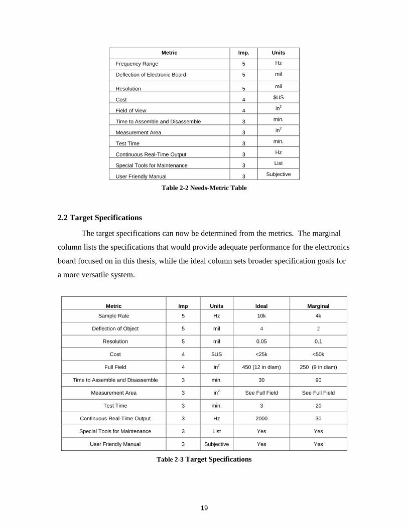
2.2 Target Specifications
The target specifications can now be determined from the metrics. The marginal
column lists the specifications that would provide adequate performance for the electronics
board focused on in this thesis, while the ideal column sets broader specification goals for
a more versatile system.
Metric Imp Units Ideal Marginal
Sample Rate 5 Hz 10k 4k
Deflection of Object 5 mil 4 2
Resolution 5 mil 0.05 0.1
Cost 4 $US <25k <50k
Full Field 4 in2 450 (12 in diam) 250 (9 in diam)
Time to Assemble and Disassemble 3 min. 30 90
Measurement Area 3 in2 See Full Field See Full Field
Test Time 3 min. 3 20
Continuous Real-Time Output 3 Hz 2000 30
Special Tools for Maintenance 3 List Yes Yes
User Friendly Manual 3 Subjective Yes Yes
Table 2-3 Target Specifications

20
Sample Rate: Military testing specifications require that a 1G sine sweep from 20-
2000 Hz be conducted to qualify electronic equipment. According to the Nyquist
Frequency Rules, it is imperative to sample at a minimum of twice that rate to ensure
aliasing does not occur. For this reason, the marginal value for Sample Rate is set at
4kHz.
Deflection of Object: This specification was set by the maximum displacement the
electronics board would have during testing. However, it would be better for the
device to be able to be compatible with multiple test structures and they might have a
greater deflection.
Resolution: The resolution is defined by the smallest measurable distance change
that can be detected by the sensor. Since the first mode of the electronic board has a
maximum deflection of about 2 mils and the second mode has a deflection of 0.5 mil,
the resolution needs to be less than these values so the modes can be captured. It was
determined that a 0.1 mil resolution would allow for the second mode to be easily
captured.
Full Field: Full Field is much like the Measurement Area specification except that it
is exclusively relating to dimensions of a full quantitative visual output of the
structure during one test. The minimums are based on the largest electronics board.
Time to Assemble/Disassemble: This specification was subjectively chosen.
Ultimately the system needs to be able to be quickly setup and torn down. It should
not take more time than it takes to mount and calibrate the existing vibration table
control accelerometers since these setups will be done in parallel.
Cost: The cost really is not the concern of this project for comparison. It has to be
low cost to gain the support of Draper Labs and be a competitive alternative to
traditional methods.
Measurement Area: This specification differs from Full Field in that it relates to
the amount of test object area that can be measured with the system through multiple
tests.
Test Time: It takes about 3 minutes to run one vibration pass of 20-2000Hz on the
shaker tables since it runs at 2 oct/min. Therefore, the optimal test time is limited by
the shaker table. The marginal spec (longest time), is 30 minutes because different

21
measurement methods are going to require data processing before subsequent test
runs can be completed.
Continuous Real-time Output: This specification quantifies the rate at which
output can be viewed during a test. The marginal value was set to 30Hz since all
high speed cameras send their images to video screen to play at this speed. If video
output is not part of the concept, this specification will be equivalent to Sample Rate.
Special Tools for Maintenance: This allows for the design to be easily fixed even if
it is intricate and has non standard parts. It also acts as a reminder to keep the
number of tools required to a minimum.
User Friendly Manual: Ensures that the hardware and software can be used by
everyone at Draper Labs and it will have an easy learning curve.
2.3 Function Diagram
The diagram below outlines the main functions for the non-contact system so
different methods can be considered for each function. This allows the design to be
formulated with consideration of all viable methods and allows it to be free from bias. For
the concept generation, the main functions that are focused on are: how the design will
integrate to the excitation source and how it will acquire the measurement data. This
decision should not be free from the other functions listed, but it is obvious that a computer
will be processing and outputting the data.
Figure 2-1 Function Diagram
Now that the main functions for the non-contact vibration system are identified,
different methods can be explored to accomplish each function.
AcquireMeasurement
DataProcess Data
Output/DisplayData
Integrate withExcitation
Source

22
2.3.1 Integrate with Excitation Source
A shaker table will provide the outside excitation to the test object to recreate the
operational environment of the test specimen. For the testing completed in this thesis, a 2-
rail hydrostatic Team Corporation slip table with an auto leveling IMIS base, and four
channel control and response will be used. See Figure 2-2 and Figure 2-3 below. This slip
table has a large plate where the test object is mounted that slides on a film of oil. These
shakers are capable of pure translational motion with very little rotational modes in the
horizontal and vertical directions [4]. For testing completed in this thesis, movement will
be in the horizontal direction.
Figure 2-2 Vibration Shaker Table Shown in Horizontal Motion Position
The actual slip table that will be used for the electronic board testing is shown
below in Figure 2-3. However, the shaker will be turned down like the illustration above.
Figure 2-3 Board Excitation Source: TA 165 Electro Dynamic Slip Table
Circuit Boardand Fixture
Oil Film
Rigid Base
ShakerSliderPlate
ShakerHead

23
The non-contact sensor could attach to the circuit board fixture or slider plate if the
sensor can withstand the 1G sine sweep from 20 to 2000Hz. The benefit of mounting
directly to the circuit board fixture is that the resonance displacements are all that will be
observed. Other options include mounting to the side rails of the vibe table or hanging the
hardware from the ceiling. The side rails are on isolation pads and should be free from
outside vibration. If the system is measuring test object displacement and is mounted on
these side rails, the movement of the vibe table will have to be subtracted off the acquired
test data. This is a less desirable option because the vibe table’s output is controlled
internally and could add an extra source for error.
2.3.2 Acquire Measurement Data
Since the entire system is hinging on the sensor that is selected, the viable sensors
need to be identified before the excitation integration is designed. This section will discuss
the benefits and limitations of non-contact sensors. These sensors utilize many different
measurement principles that allow them to capture the target objects dynamic behavior
without physically touching it. Most non-contact sensors will only work with a few types
of target surfaces and materials. For the application of measuring electronics equipment, it
would be desirable to have a sensor that worked with the multitude of surfaces and
materials that make up a populated printed circuit board (PCB).
The viable sensor options that do not run on optical principles are inductive
proximity (eddy current), and capacitive. Optical sensors allow for a lot more versatility in
test measurement but this comes at an increased cost. Although optical methods are
becoming more common, a quick survey of sensors listed for vibration testing mention
little to nothing about these sensors and their unique capabilities. The optical sensors that
could be used in this product are holographic interferometry, laser Doppler velocimetry,
laser triangulation, or area scaling. All of these measurement methods are discussed
below. This background will then be matched with options from the other functions to
form three concepts for the Non-Contact Vibration System.
2.3.2.1 Inductive Proximity (Eddy Current)Non-contact displacement sensors using eddy current technology are known as
inductive proximity sensors. These sensors make precise static and dynamic

24
measurements of metal targets and thickness measurements on conductive material backed
by metal. These sensors utilize a high- frequency magnetic field which is generated by
passing a current through a coil in the sensor head [5]. When a metal target is introduced
to this field, electromagnetic induction causes an eddy current to travel on the surface of
the target, changing the impedance of the sensor head coil [5]. When a target comes closer
to the sensor’s head, the oscillation amplitude decreases and the phase difference from the
reference waveform increases. The sensor detects the change in amplitude and phase to
obtain a value proportional to the distance between the target and the sensor head [5].
Figure 2-4 Keyence Inductive Proximity Sensors [5]
The target size is an important consideration when selecting this type of a sensor.
If the target is smaller than the sensor head, measurements can be effected by other
conductive targets near by. Shielded sensors try to reduce these ill-effects. Proximity
sensor’s main use is to measure the space between the probes head and a conductive
material since non-conductive materials in the gap does not effect measurement.
Proximity sensors have a very limited measurement range and have to be placed extremely
close (less than a tenth of an inch) to the test specimen requiring mounting methods to be
very precise. A benefit over the capacitive sensors that are discussed next is that they are
highly insensitive to oil, dirt, dust, moisture, and interference fields [6, 7].
For the application of electronic board’s displacement measurement, the conductive
material must be present on the surface and not hidden within the layers of the PCB unless
calibrated measurement is going to be performed. This could cause problems in

25
determining places on the board where displacement measurements can be made.
Calibration of sensors could make testing tedious and time consuming if each point on a
populated board has a different metal consistency. Also, during bare frame electronic
board tests, the frames are thinner than the penetration depths of the sensors so a build up
of eddy currents on the back of the board could lead to false readings.
2.3.2.2 CapacitiveNon-contact capacitive displacement sensors measure distances, lengths, dimensions,
and positions of any electrically-conducting targets (e.g. metals) [6, 7]. This sensor’s
principle of operations is that a capacitor is formed when two parallel plates are brought
near each other and a charge is placed on one of the plates. Current then flows across the
gap between the plates and the amount of current is determined by the voltage, area of the
plates, and the material the separates the plates [6].
Figure 2-5 Capacitive Sensor [6]
Unlike proximity sensors, the target thickness is not important for capacitive
sensors since the charge resides on the surface of the conductor. Also, changes in target
material do not affect the sensor’s performance as long as it is conductive. With proper
calibration, a technique called fringing can be used to measure the displacements of non-
conductive materials. Fringing involves inserting the non-conductive target between the
sensor and a conductive reference surface [6]. The presence of the non-conductive
material’s dielectric constant will alter the air medium around the sensor allowing for the
d
Capacitance
Target
Sensor

26
non-conductive target’s properties to be measured [6]. A capacitive displacement sensor
requires a clean environment. Dirt, dust, or water in the measuring gap can influence the
measurement signal [7].
2.3.2.3 Holographic InterferometryHolography uses the coherent light produced by lasers to reconstruct 3D objects.
The unique characteristic of holography is that it will record both the phase and the
amplitude of the light waves that are reflected off of the object to a photographic surface
[8]. The photographic surface responds to the intensity of the light in the form of phase
information that can be interpreted when it is compared with the reference beam and
converted into variations in intensity [8]. The reference wave and the scattered light waves
from the object produce an interference pattern on the photographic film called fringes.
Figure 2-6 Holographic Interfermetric Setup
When sequential holograms are compared, small changes in the shape of the test
object can be seen and measured through interfermetric techniques. Through Real-time
holography, displacement fringes of an object under vibration can be viewed on a video
screen to locate resonant modes. Then a time-average technique of holographic
interferometry can be used to dwell at the identified natural frequencies and record a
ObjectmirrorBeam splitter
Electronic board
Referencemirror
Lenses
Lenses Camera
ImageProcessing
Monitor
Photographic plate

27
quantitative output of the deflections of the object with a resolution of one-half the
wavelength of the laser used.
Because this method looks at how the object has changed from the null position
captured by a video camera, the imperfections of lenses and mirrors do not effect
measurements [8]. The greatest benefit of this technique is that the entire test object can be
measured, not just discrete locations like almost every other vibration sensor considered.
The resolution of this method is half the wavelength of the laser light used; this is about 10
micro-inches with an argon ion laser [9]. Since the fringes are set by the wavelength of the
laser used, scaling the testing conditions is the easiest way to keep fringes readable without
doing more complex techniques to acquire data. It is hard to read displacement maps with
more than about 20 or 30 fringes (~0.25 mils). With such low displacement levels needed,
the excitation source for this method is usually just an acoustic speaker. This test is viable
for non-contact testing but if the system does not perform linearly, the excitation scaling
will lead to erroneous characterization of dynamic performance.
2.3.2.4 Laser Doppler Vibromet erLaser Doppler Vibrometry (LDV) uses a focused laser beam to measure the
velocity at a discrete point. The velocity is calculated by using the Doppler shift between
the incident light and scattered light returning to the measuring device [10]. The laser
beam is continuously scanned over the vibrating object and after demodulation of the data,
mode shapes can be determined.
The LDV has some clear advantages over other non-contact measurement methods
because there is considerably less data storage and processing required as compared with a
full field measuring instruments like real-time and time-average holography [11]. The
LDV is completely non-contact and is unaffected by environmental conditions or surface
properties. Also, thousands of points can be successively measured, and multi-channel
instrumentation is not required [11]. The disadvantages include “speckle drop out” (the
speckle noise can distort LDV signal), line of site required from laser head to the target, the
time it takes to run the test and then demodulate the data, and the cost of an LDV system
[11].

28
2.3.2.5 Laser Triangulation
A laser triangulation sensor is a highly accurate measurement technique using a light
emitting element, and a position sensitive detector (PSD). A charge-coupled device, CCD,
is also used in the newer displacement sensors instead of the PSD. The triangulation
sensor incorporates a semiconductor laser that has its beam focused by a lens as it leaves
the sensor head [5]. The beam is then reflected off of the surface of the target and back
through a receiving lens. The light beam is focused on the PSD or CCD forming a beam
spot and the movement of the beam spot is used to calculate the displacement [5].
Figure 2-7 Laser Triangulation Sensor [5]
A draw back of most laser triangulation sensors is that they require a highly reflective
surface or a highly diffuse surface. This requires painting or sticking something white at
the point of measurement which is undesirable. Keyence has a newly released laser
triangulation sensor, LK-11, that can measure multiple surface types and colors. This
sensor would allow for a more versatile system without mass loading the electronic board
with white dots.

29
2.3.2.5 Area Scaling
This measurement option has not been used in vibration testing but the idea seems
like a revolutionary method for measuring displacements in a non-contact manner. The
area scaling method uses a simple technique of relating the in-plane displacement of an
object to its area growth or reduction in the recorded camera images. For example, if one
holds an object in front of them and then moves it towards or away from their face, its size
grows and shrinks. This technique is much like how we can tell the distance of objects by
their relative sizes. The area scaling method looks at the scaling effects of a discrete area
on the electronic board due to the planar displacements seen in vibration testing. The
discrete area can be an object feature or simply a labeling dot that is just stuck onto the
object’s surface at the area of interest. The final output of the electronic board’s
quantitative displacements and mode shapes during vibration testing can be related to how
much the discrete area changes. The picture below shows the variables for this technique.
Figure 2-8 Area Scaling Technique Variables
The camera sensor has a height and width that is determined by the size and
number of pixels present on the CCD sensor. Pixels average about 15 µm for a standard
digital camera CCD chip. The denser the pixel counts, the larger the sensor area if the
pixel dimensions stay constant. The focal length, f, is the distance from the lens to the
sensor. The focal length can be changed by swapping out the lens on the camera. The
working distance, D, is the distance from the lens to the object. Also, the object (scene)
CameraSensor
h
w
D
f
W
H
Scene
Lens

30
has a given height and width, H and W. The scene is scaled to the size of the CCD chip
which has its own height and width, h and w respectively. The entire electronics board
could describe the scene dimensions or just a part of the object could be focused in on for a
better displacement resolution. As the scene displaces towards or away from the lens, the
working distance shortens or lengthens which equates to a change in the discrete area of
the scene.
Since the displacements that are seen in a vibration test of the electronics boards are
on the order of a thousandth of an inch, a change in area will not be able to be viewed by
the naked eye during testing. Digital processing is required to look at each frame’s image
pixel by pixel. Edge detection methods could then be used to find the discrete area and
subsequent frame by frame comparisons of these images will show the growth and
reduction of the known areas of interests. This optically viewed change in area can be then
related to the deflection of the object.

31
Chapter 3 Concept Genera tion
3.1 Concept 1: Holographic Interferometry
The first concept involves building a holographic interfermetric system to record
the displacement fringes of the electronic boards under vibration testing. This method was
chosen because it allows for a full field output of the object under testing even though it
would involve a complex optics setup. Since military testing specifications require a
certain test, it is questionable to scale testing parameters to achieve a lower displacement
level. A simple study was completed and reported in Section 3.1.2 to see if image
processing could pick out the fringe contours without scaling the excitation levels in the
test. The benefits and limitations of this concept are also discussed.

32
3.1.1 Displacement Fringes
During the 20-2000 Hz sine sweep, the fringes of the electronics board’s
displacements are recorded and sent to a monitor. Because of the amount of data being
taken in, displacement maps cannot be recorded for the entire 20-2000 Hz test. Instead, a
method called Real-time holography is used to sweep through all the frequencies and the
natural frequencies are identified visually on a monitor. Once the natural frequencies are
identified, then time average techniques can be used to dwell at the natural frequency of
interest and output a displacement map corresponding to the structure’s mode. This results
in a full field output of displacements but a very long test time. See Figure 3-1 below
shows how the test object’s deflections are seen as displacement contours.
Figure 3-1 Interference Fringe Example [8]
3.1.2 Unscaled Testing Study
The goal of this study is to determine if unscaled testing can be used with
holographic interfermetric techniques. The contour map will have a fringe for every 0.26
microns or 0.001mils3 of displacement perpendicular to the lens of the camera. See Figure
3-2 for an idealized representation of how the fringes could be discerned pixel by pixel. In
actuality, it will take more than one pixel to read a fringe but this will do a decent job of
estimating the maximum number of fringes that can be interpreted.
3 Argon Lasers are most commonly used and they have a 514nm wavelength.
DisplacedBoard
Fringe
DestructiveInterference
HologramConstructiveInterference

33
Figure 3-2 Fringe Contours on Pixel Grid
Since the electronics board first mode occurs in the center of the board with a
maximum displacement of two thousands of an inch, the contours will look similar to the
image on the right in Figure 3-2. If the 1-G sine sweep is not scaled during vibration
testing, there would be approximately 200 displacement fringes. Now assuming the
densest fringe scenario where each fringe only takes up one pixel and only one pixel is
between fringes, the question is: What is the densest area of fringes that can be discerned
with a 0mil to 2mil difference in displacement? The answer is dependent on the resolution
of the camera recording the fringe maps. With an 800x600 resolution, the 200 fringes will
require 399x399 pixels. If the board area under observation is 3.5x 2.625 inches, then the
displacement must occur over a target area greater than 2.33 x 1.75 inches in order for it to
be adequately read. Increasing the resolution of the camera sensor to 4k x 4k would allow
the 2 mil displacement difference to occur over a minimum area of 0.35 x 0.35 inches.
This quick approximation does not take into account that fringes will occur more
than one pixel apart and that fringes may have a width greater than one pixel. Therefore,
this estimation could be off by as much as an order of magnitude. However, this study
does show that this method would require a reduced G level for the vibration test for
cameras with poor resolution. If a camera with greater than 4k x 4k resolution were used,
2D=λ/2
D
D
pixel

34
there is a high possibility that unscaled testing could occur but more in depth testing would
need to be performed to see if other variables influence required resolution.
3.1.3 Concept 1 SummaryBenefits
• Full Field• High Resolution
o 0.26 microns or 0.001 mils• Real Time Output
Limitations• Intensive Signal Processing• Hard to decipher large deflections
o Scaled testing?• Have to dwell at natural frequency to get quantitative output• Complex Optics Setup
3.2 Concept 2: Area Scaling
The area scaling idea was chosen for the second concept because it is a
revolutionary non-contact sensor method. If a test object’s small deflections can be
decoded by slight changes in discrete areas present on the object, it could provide a
technique for full field measurement with merely a high speed camera and some image
processing tools. As discussed in Chapter 2, the area scaling method looks at the size
growth and reduction of a discrete area on the electronics board due to the planar
displacements seen in vibration testing. The final output of the electronics board’s
quantitative displacements and mode shapes during vibration testing can be related to
how much the discrete area changes. Since the displacements are on the order of a
thousandth of an inch, it is questionable whether CCD technology is adequate to capture
the slight area change. A test using current lab resources was completed to check the
feasibility of this concept and look at the image processing techniques available to
capture the area changes in the recorded images. Results of the testing and further
analysis are reported in this section.

35
3.2.1 Area Scaling Concept Testing
A high speed digital camera was available for testing so a feasibility test was run
to see if the displacements could be captured by the growth and reduction of a
predetermined discrete area on the board with the equipment available. Other testing
goals included evaluating setup issues and image processing techniques using MATLAB.
The camera being used is a Red Lake CR2000 high speed CCD camera. It can
record up to 2000 frames/second at a resolution of 512x192. A better resolution of
512x384 can be acquired if the test is run at 1000 frames/second. Ultimately, a camera
that could sample up to 4000Hz would be needed to capture the entire 20-2000Hz sine
sweep vibration test but for the purpose of this study, it was not an issue.
For the test, a ¾ inch diameter labeling dot is placed in the center of the electronic
board since max displacement occurs there. See Figure 3-3 for the dot location.
Figure 3-3 Electronic Board with Discrete Area Label
Labeling Dot

36
The electronic board is secured in the aluminum test fixture and mounted to the
vibe table. Figure 3-4 below shows the test setup.
Figure 3-4 Top View of Testing Diagram
When the labeling dot displaces toward the camera, the area of the dot will grow
in the field of view (FOV). In order to capture the most area growth, the camera was
zoomed in until almost the entire scene was the labeling dot. Enough room was left at
the top and bottom of the labeling dot that a change in area could be seen.
Figure 3-5 Testing Field of View
TOP VIEW
Shaker
Electronicboard
Camera
fixture
1.19”
0.885”0.75”
37
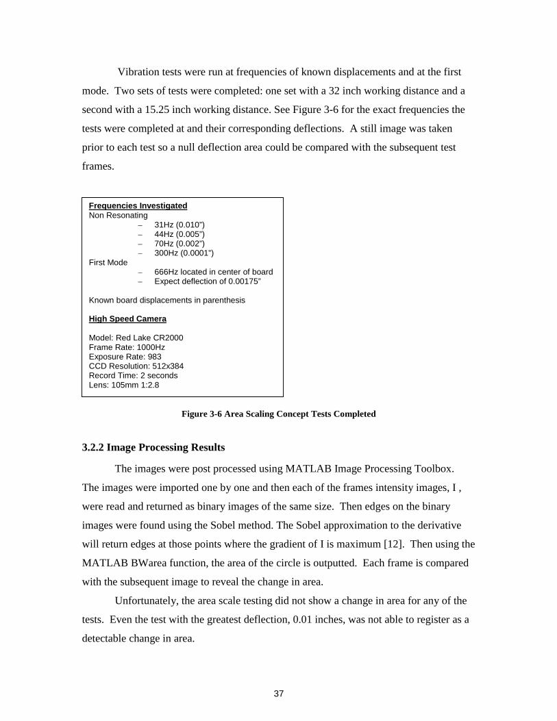
Vibration tests were run at frequencies of known displacements and at the first
mode. Two sets of tests were completed: one set with a 32 inch working distance and a
second with a 15.25 inch working distance. See Figure 3-6 for the exact frequencies the
tests were completed at and their corresponding deflections. A still image was taken
prior to each test so a null deflection area could be compared with the subsequent test
frames.
Figure 3-6 Area Scaling Concept Tests Completed
3.2.2 Image Processing Results
The images were post processed using MATLAB Image Processing Toolbox.
The images were imported one by one and then each of the frames intensity images, I ,
were read and returned as binary images of the same size. Then edges on the binary
images were found using the Sobel method. The Sobel approximation to the derivative
will return edges at those points where the gradient of I is maximum [12]. Then using the
MATLAB BWarea function, the area of the circle is outputted. Each frame is compared
with the subsequent image to reveal the change in area.
Unfortunately, the area scale testing did not show a change in area for any of the
tests. Even the test with the greatest deflection, 0.01 inches, was not able to register as a
detectable change in area.
Frequencies InvestigatedNon Resonating
– 31Hz (0.010”)– 44Hz (0.005”)– 70Hz (0.002”)– 300Hz (0.0001”)
First Mode– 666Hz located in center of board– Expect deflection of 0.00175”
Known board displacements in parenthesis
High Speed Camera
Model: Red Lake CR2000Frame Rate: 1000HzExposure Rate: 983CCD Resolution: 512x384Record Time: 2 secondsLens: 105mm 1:2.8

38
3.2.3 Area Scaling Analysis
Since the results of the testing proved current equipment could not capture the
minute deflections of the electronics board, a second look was taken to determine what
sensor resolution is required for this method to work. The concept parameters are seen in
Figure 3-7 below.
Figure 3-7 Test Parameters
where f is the focal length, D is the working distance with the board in the null position,
D’ is the working distance in the fully deflected state, and d is the deflection of the board.
The Camera sensor has a width, w and the electronics board has a width, W. Since the
camera sensor has a larger resolution horizontally, the width of scene and sensor is all
that will be used in determining the minimum detectable deflection. The amount the
electronics board scene is scaled by in order to be represented on the camera sensor is just
a relation between their widths as seen in Equation 3-1.
Equation 3-1 273.018.1
32256.0 ===WwScale
ElectronicBoard
f D
CameraSensor
D’ d
Ww

39
The scaled amount can now be used to relate the pixel resolution to the object
resolution (smallest viewable feature).
Equation 3-2 resobj
widthpixScale_
_=
inchesresobj 000172.000063.0*273.0_ ==
To get accurate resolution, two pixels are needed to represent the area edge [13].
See figure below to view assumptions that will be used in calculating the minimum
detectable deflection.
Figure 3-8 Minimum Detectable Dot Growth
Since two pixels correspond to an object resolution of 0.0044 inches, the 0.75
diameter dot will have to grow by 1.2% or to a diameter of 0.7588 inches to be seen.
Now the question is how much does the board have to deflect to achieve this amount of
growth? To solve for the growth a simple geometric relationship is used to solve for D’
in Equation 3-3 below.
Equation 3-3 '
)0044.*2(219.1
13386.42
32256.0
'
)_*2(22DD
resobjW
f
w −=→
−=
D’ = 15.02 inches
d = D - D’ = 0.23 inches
Null Dot Size
Dot at MinDetectableDeflection
2 pixels

40
The minimum deflection that will be able to be seen is 0.23 inches with the
current equipment and setup. In order to achieve a displacement resolution equal to the
marginal specification of 0.1mil using the same setup, a 34kx34k resolution camera
sensor is required.
High speed cameras have just recently been released with over a 1.5kx1k
resolution.4 While, optical techniques could possibility compensate for lower resolution
sensors, there is hope with the ever-increasing CCD and CMOS technology that this
could be a viable method in the future.
3.3 Concept 3: Displacement Sensor GridThe final concept involves using a grid of displacement sensors that can be
scrolled down the face of the electronics board. This option does not require a very
complex setup but it will capture discrete locations on the surface of the board. The
displacement sensor that has been chosen for the concept is a laser displacement sensor.
Two laser sensors exist that could be used in this design. If this concept is chosen, sensor
selection testing would have to be completed.
Proximity sensors were also considered but because they require a metal target, it
was determined they would be too restrictive on the target objects that could be tested
and could make interpretation of test results hard since copper layers exist within the
printed circuit boards. Also since the bare frame aluminum electronic(s) board is thinner
than the penetration depth of all proximity sensors considered, eddy currents build up on
the back of the metal could give false readings.
4 Red Lake HG-100K camera has a 1504x1108 resolution and can sample up to 1000 frames/second.

41
The figure below shows the idea of the sensor probes capturing the board
displacements through voltage output during vibration testing.
Figure 3-9 Displacement Sensor Grid Example
Since the laser displacement sensors cannot undergo more than 55Hz, they would
have to be mounted from the shaker table rails that are on isolation pads. The hardware
would not only have to suspend the sensors in front of the board, but it would have to
incorporate some sort of a vertical rail so that multiple locations on the board could be
captured.
Table 3-1 shows the specifications on the two laser displacement sensors under
consideration.
LK-11 Sensor Head LC-2440 Sensor Head
Reference Distance 10mm (0.39”) 30mm (1.18”)
Measuring Range ±1mm (0.04”) ± 3mm (0.12”)
Resolution 0.2µm (0.008 mil) 0.2µm (0.008mil)
Sample Rate 7812.5 Hz 50,000 Hz
Target Surface Any White: Diffuse Reflective
ElectronicBoard
LaserDisplacementSensors

42
Table 3-1 Displacement Grid Sensor Comparison
3.3.1Concept 3 SummaryBenefits
• Easy Setup• Simple Equipment• Resolution <1µm• Large Frequency Range
Limitations
• Measures Discrete Points• Limited Measuring Range• Must Mount to Shaker Table Rails
o Could introduce error
3.4 Concept Comparison
The three concepts have each been assigned ratings based upon how well they
meet target specifications. These ratings are then multiplied by the specification’s
importance to reveal a weighted score. The scores for each product are summed giving a
general way to compare the effectiveness of each concept at accomplishing the design
goals. The concept comparison matrix is below in Table 3-2.
HolographicGrid of
DisplacementInterferometry
Area ScalingSensors
Selection Criteria Imp. Rating Score Rating Score Rating ScoreSample Rate 5 4 20 2 10 5 25
Deflection of Board 5 3 15 1 5 5 25 Resolution 5 4 20 1 5 5 25
Cost 4 3 12 4 16 3 12 Full-field 4 5 20 3 12 2 8
Time to Assemble/Disassemble 3 2 6 5 15 4 12Measurement Area 3 5 15 3 9 4 12
Test Time 3 3 9 4 12 5 15 Continuous Real-Time Output 3 5 15 3 9 3 9Special Tools for Maintenance 3 3 9 5 15 4 12
User Friendly Manual 3 5 15 5 15 5 15TotalScore 156 123 170
Rank 2 3 1

43
Table 3-2 Concept Comparison Matrix
The matrix shows that the Displacement Grid Concept will achieve the best result
of reaching the target specifications. Second is the Holographic Interfermetric method
and third is the Area Scaling method. Based on these results and the support of Draper
Laboratory, the Grid of Displacement Sensors will be the concept developed. Chapter 4
will cover the prototype hardware and software design, as well as, sensor selection
testing.

44
[THIS PAGE INTENTIONALLY LEFT BLANK]

45
Chapter 4 Prototype Design and TestingThis chapter will delve into the hardware and software design for the
displacement sensor grid system. The goal of this round of design work is to create a
prototype system that will test the capabilities of the Keyence LC-2440 and LK-11
displacement sensors. While the hardware will primarily be designed for the sensor
selection testing, it must be easily modified for the final multi-sensor system. Sensor
selection testing and results will be discussed and by the end of this chapter, a sensor will
be chosen for the final design. An evaluation of the prototype hardware will also be
presented.
4.1 Mechanical DesignThe hardware needs to accomplish the following functions: mount to the slip table
side rails, span from rail to rail, provide an interchangeable mount so both the LC-2440
and LK-11 sensors can be secured at their reference distance, and have at least one

46
unconstrained degree of freedom so sensors can be scanned over the surface of the
electronic board. See picture below for shaker table diagram in Figure 4-1.
Figure 4-1 Shaker Table Sketch
4.1.1 Mounting Options
The vibration table has two 4-inch wide rails on each side. Since the sensors are
going to need to be positioned horizontally (towards or away from the electronic board),
the system needs to be easily adjustable in the z-direction. The entire system and sensors
will be suspended from these mounting devices so whatever is chosen needs to be sturdy
and provide an easy attachment scheme for the sensor cross bar.
Five inch wide drill press vises will be used for the rail mounting function
because they fulfill the required functions, they are low cost, and will require little
modification.
EA Fixture withElectronic Board
4” Wide SideRails
motion
Shaker
x
y
z
VerticalRailAttacheshere
Can Clamp ShakerTable Rails Here

47
Figure 4-2 Shaker Table Mounting Scheme: Drill Press Vise
Two, quarter inch aluminum sheets will hang perpendicular to the vise’s
mounting surface by way of an L-Bracket. These aluminum verticals will hang inside the
vibe table rail walls to provide the mounting surface for the cross bar. The cross bar
attachment scheme will have to allow the cross bar to be moved in the vertical, y,
direction.
4.1.2 Vertical Movement
The vertical movement of the cross bar can be accomplished in a variety of ways.
Holes can be drilled at discrete distances from each other allowing for a precise
placement of the cross bar and sensors. This option would ensure that the point on the
electronics board being captured by the sensor is known but it would limit the number of
locations that could be investigated by the system.
Figure 4-3 Discrete Vertical Movement: Holes
Another option is to incorporate a slot along each rail so infinite points in the
vertical direction can be investigated on the board. This would allow for an infinite
number of measurement positions.
Rail
vise
Cross barElectronicboard
Discretemovement
y
x

48
Figure 4-4 Vertical Movement: Slot
Since the vertical slot will not limit the vertical position of the cross bar, it will
provide the greatest test versatility and was chosen for the system. A nut and bolt will be
used to fasten the cross bar in a particular location of the slot and a digital read out
(DRO) will be attached to one of the verticals so the exact location of the sensor will be
known.
4.1.3 Sensor Mount
A mount needs to be designed to attach the LK-11 and LC-2440 to the cross bar.
Since their output is going to be compared, they should capture the displacements of the
same spot on the board. However, they do not have to be mounted at the same time.
Since the LC-2440 has to be mounted 30mm from the surface of the board compared to
the LK-11’s 10mm, a simple bracket mounting the sensors horizontally was designed.
See illustrations on the next page.
Rail
Vise
Cross barElectronicboard
Slot
y
x

49
Figure 4-5 Sensor Mount in Both Sensor Configurations
The prototype hardware system that was built for sensor selection testing is below
in Figure 4-6.
6” DRO Scalewill allow forprecise verticalmovement
LaserDisplacementSensor
Adjustment slots allowfor exact fit in theinside walls of the sliptable
L-Bracketsattach to end of5” Drill PressVises
Sensor bracket can beused for both LK-11and LC-2440 byswitching mountingholes
Slots allow forinfinite mountingheights
y
z x
Cross bar
Keyence LC-2440Displacement Sensor
Sensor mount
Keyence LK-11Displacement Sensor

50
Figure 4-6 Sensor Selection Hardware Design
Figure 4-7 Sensor Selection Hardware Design with Vises
4.2 Software DesignThe final system needs to not only obtain the laser output, but it needs to analyze
it as well. For this reason, the most efficient choice is to have both the data acquisition
software and analysis software written in the same code. It was decided that MATLAB
would be used because a data acquisition and analysis package was available.
A simple program was written to acquire the laser output at a specified sample
rate from a National Instruments NI DAQ-1200 card and save it as a “.daq” file for post
processing. A picture of the program can be seen in Figure 4-8 below.
Figure 4-8 Data Acquisition MATLAB Program: Laser Vibe Test 1.0

51
4.3 Sensor ComparisonThe Keyence LK-11 sensor head and LK-3101 controller sell for around $5900
while the LC-2440 Sensor and LC-2400 Controller sell for approximately $9300. The
main advantages of the LK-11 sensor is that it can read the displacement of any surface
type while the LC-2440 can only read a specular diffuse (white) target. Since multiple
sensors would be incorporated into the final system for shorter test times, the LK-11
sensor would be best suited because it is one-third the size of the LC-2440 allowing four
sensors to easily fit the width of the electronic board. The LC-2440 sensor system would
be better, however, for a more versatile vibration measurement system because it can
sample up to 50kHz while the LK-11 system has a maximum sample rate of 7812.5 Hz.
Sensor performance during vibration testing will help determine the best sensor for the
final system.
4.3.1 Sensor Selection TestThe purpose of this test was to assess the capabilities of the laser triangulation
sensors for electronics board vibration testing, evaluate the hardware and software
design, and ultimately compare the results of the LK-11 sensor with the LC-2440 sensor
to determine which would be used in the final vibration measurement and analysis
system.
4.3.1.1 Test SetupThe electronic board bare frame was mounted in an aluminum fixture that bolts
down to the vibration table. See Figure 4-9 below.
Figure 4-9 Electronic Board Test Setup
ControlAccelerometerLocations
Connector
Vibration Fixture
Pico EndevcoPiezoAccelerometer

52
The control accelerometers are averaged and used by the table to ensure the board
is held under a c-onstant 1-G acceleration during the sine sweep. The center mounted
accelerometer verifies that each test produces the same electronic board response and
since the accelerometer is capturing the same point as the laser sensor, it can be used later
to validate the laser displacement output. See Figure 4-10 below for complete hardware
setup.
Figure 4-10 Hardware Test Setup
4.3.1.2 Sensor SetupThe Keyence LK-11 displacement sensor with the LK-3101 controller requires
24V DC input and will output a voltage of ± 10V. The National Instruments DAQ 1200
board has an input voltage limit of ± 5V so a voltage divider circuit was built to cut the
laser output voltage in half. A wiring diagram for the LK-11 test can be seen in Figure
4-11.
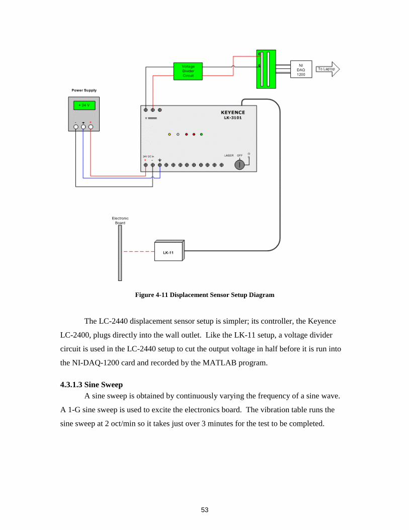
53
Figure 4-11 Displacement Sensor Setup Diagram
The LC-2440 displacement sensor setup is simpler; its controller, the Keyence
LC-2400, plugs directly into the wall outlet. Like the LK-11 setup, a voltage divider
circuit is used in the LC-2440 setup to cut the output voltage in half before it is run into
the NI-DAQ-1200 card and recorded by the MATLAB program.
4.3.1.3 Sine SweepA sine sweep is obtained by continuously varying the frequency of a sine wave.
A 1-G sine sweep is used to excite the electronics board. The vibration table runs the
sine sweep at 2 oct/min so it takes just over 3 minutes for the test to be completed.

54
Figure 4-12 Vibe Table Sine Sweep Representation
The displacement of the vibration table during the sine sweep will be seen as a
downward sloping line on a loglog plot following Equation 4-1 below.
Equation 4-1 2
*8.9f
aYo ≅
where Yo is the single amplitude displacement in inches, a is the acceleration in G’s and f
is the forcing frequency in hertz.
The slip table displacement will have to be subtracted off of the laser
displacement output to get the electronic board’s modal displacement. See Figure 4-13
below for the vibe table displacement during the 1G sine sweep from 20-2000Hz. Please
note that Figure 4-13 depicts the single amplitude displacement or the maximum positive
amplitude of the sinusoidal motion. See figure below.
Figure 4-13 Vibration Table Sine Sweep Displacement vs. Frequency
1
Time (s)
Acc
eler
atio
n (G
)
-1
LogLog Plot Linear Plot

55
4.3.2 Electronic Board Accelerometer OutputThe maximum displacement of the first natural frequency of the electronic board
occurs at the center of the board so the center mounted accelerometer will pick up the
board’s max dynamic response around 660 Hz and 80 G’s (1.8 mil). The typical
accelerometer output for the 1G sine sweep of the electronic board under investigation
can be seen below.
Figure 4-14 Typical Accelerometer Output for Electronic Board
4.3.3 Laser Displacement OutputThe laser output is voltage vs. test time. This data can be easily converted to
displacement versus time with a conversion factor. However, only a rough estimate of
displacement versus frequency can be shown at this point using the test time and the
2oct/min vibe table sweep speed. A more accurate way of determining frequency of the
data, will be shown later in Chapter 5, where an algorithm will actually step through the
laser output and read the frequency content directly from the sine wave zero crossing
times.
Typical Electronic Board Sine Sweep Response
1st Mode78G’s, 657.6Hz
2nd Mode3.3 G’s, 1448 HzCenter Accel
ControlAccel 1
ControlAccel 2
Frequency (Hz)
Acc
eler
atio
n (G
’s)
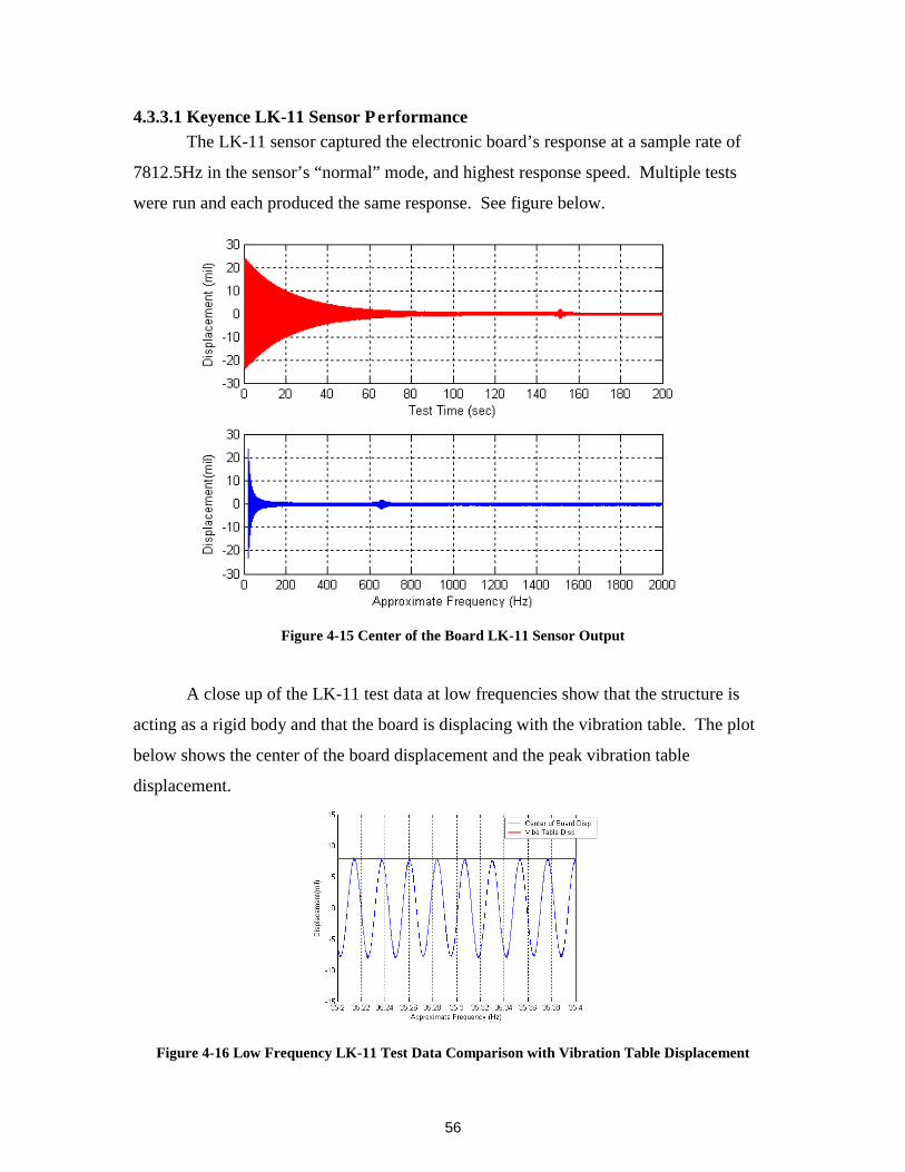
56
4.3.3.1 Keyence LK-11 Sensor PerformanceThe LK-11 sensor captured the electronic board’s response at a sample rate of
7812.5Hz in the sensor’s “normal” mode, and highest response speed. Multiple tests
were run and each produced the same response. See figure below.
Figure 4-15 Center of the Board LK-11 Sensor Output
A close up of the LK-11 test data at low frequencies show that the structure is
acting as a rigid body and that the board is displacing with the vibration table. The plot
below shows the center of the board displacement and the peak vibration table
displacement.
Figure 4-16 Low Frequency LK-11 Test Data Comparison with Vibration Table Displacement

57
The board should hit its first resonant mode around 660 Hz with a displacement
just below two mils. The bump in Figure 4-15 in this frequency region is evidence that
the LK-11 sensor picked up the board’s first mode. A close up of this region of the test
data with a comparison to the vibration table displacement is below in Figure 4-17.5
Figure 4-17 Comparison of Vibration Table and Board Displacement in the First Mode Region
The LK-11 sensor captured the first mode displacements of the electronic board
quite well. The only area that is of concern is the noise in the LK-11 output that masks
the second mode and could limit the resolution of the final vibration system if this sensor
is chosen. See Figure 4-18 for a plot of the sensor noise.
5 The center of the board displacement as captured by the lasers refers to the displacement of the board andthe vibration table. The actual board displacement can be found by subtracting the peak vibration tabledisplacement from the peak board displacement.

58
Figure 4-18 LK-11 Sensor Test Noise
4.3.3.2 LC-2440 Sensor PerformanceThe LC-2440 is a larger and much more sensitive sensor but it has to have a
diffuse reflective target (white). During testing it was set to a sample rate of 20kHz and
the laser beam was focused on a white labeling dot in the center of the electronic board
(the same point on the board that was captured by the LK-11 above). Figure 4-19 shows
the LC-2440 test data. It can easily be noticed that more noise exists in the LC-2440
sensor data compared to the LK-11 data presented in Figure 4-15.
Figure 4-19 Center of the Board LC-2440 Sensor Output

59
Unlike the LK-11 sensor, it is not apparent at this viewing resolution that any of
electronic board’s resonant modes were captured by the sensor. An up close look at the
first mode region does in fact reveal that the sensor’s mode was captured.
Figure 4-20 LC-2440 Sensor Output: First Mode Region
4.4 Sensor SelectionThe LK-11 sensor was chosen for the final system. Based on test data, the sensor
provides less output noise and has the distinct advantage over all other displacement
sensors in that it can read all target materials. It is a huge drawback that the LC-2440
system requires a white dot to be stuck on the test specimen, especially since the purpose
of this thesis is to develop a measurement system that does not mass load the structure
during testing. The LK-11 is more compact and will allow up to four sensors to be
stacked side by side to measure the electronic board’s displacements. In comparison, the
LC-2440 would only fit two sensors, requiring twice as many tests at around the same
cost as the four LK-11 sensors. Both sensors provide promising results of the first
resonant mode of the electronic board but because of noise, the second mode is not
distinguishable. Work will be done in the next chapter to try and reduce the noise level
of the LK-11.
4.5 Hardware EvaluationThe hardware worked quite well for the sensor selection test. The small slot
adjustments on the crossbar and the vertical movement slots on the vertical rails allowed
for exact placement of the laser beam in both the horizontal and vertical directions.
During testing, since only one sensor was used, the levelness of the crossbar was

60
neglected. However, when more sensor heads exist, there will be a need to ensure the
cross bar is level.
The hardware setup had a natural frequency of 16 Hz with the LK-11 (80 gram)
sensor attached and 15.5Hz with the heavier LC-2440 (250g) sensor. In order to test how
much vibration the sensors saw during the sine sweep and to ensure the vibration table
rails were isolated from vibration during the test, an accelerometer was placed near the
laser sensors to capture the vibration in the horizontal direction.
Figure 4-21 Hardware Accelerometer Location
If these sensors were not properly isolated and the sine sweep provoked the
system’s natural frequency, false displacement readings might have been recorded when
in actuality, it is the sensor head itself displacing. Figure 4-22 shows the accelerometer
output for the hardware with the LK-11, the hardware with the LC-2440, and the center
of the electronic board response during the sine sweep.
HardwareAccelerometerMounted Here

61
Figure 4-22 Comparison of Sensor Head Displacement with Center of the Board Displacement
The sensor’s displacement stays about an order of magnitude below the
electronics board displacement. The additive/subtractive sensor displacements are
negligible in comparison to the board displacements the sensors will measure in the
board’s first mode region. However, it is evident that the heavier LC-2440 hardware
configuration pushed the sensor head horizontal vibration amplitudes down. Since the
LK-11 sensors will be used in the final system, actions should be taken to ensure the
system is weighted enough so false displacement readings do not occur and a better
system resolution can be obtained.

62
[THIS PAGE INTENTIONALLY LEFT BLANK]

63
Chapter 5 Final Design and TestingThe four sensor hardware design was built and a MATLAB software package was
written to acquire and fully analyze the electronics board displacement data during
vibration testing. In order to evaluate the Non-Contact Laser Vibration Measurement and
Analysis System’s performance, two rounds of vibration tests were completed. Each test
captured an 8x4 grid of electronics board displacements during a 20-2000Hz sine sweep
at 1-G on the shaker table. The final hardware design, test procedures, and test results are
presented in this chapter. The analysis software package was written to quickly process
the raw voltage output from the displacement sensors and create a movie file displaying
the electronics board’s modal displacements. The five step analysis program will be
explained as the data analysis methods are discussed.
5.1 Final Hardware Design
The final hardware design was based on the prototype evaluations and the
required modifications to incorporate the four LK-11 sensors. Since the original

64
electronics board vibration fixture was going to be used, the four sensor mounting
scheme had to be carefully designed. The final design can be seen below.
Figure 5-1 Final Hardware Setup
THK Linear Bearings were added for smoother vertical movement and discrete
positioning. The system uses a unique setup to horizontally position the cross bar in 1cm
increments. The THK Rails came with ¼ inch diameter bores every 2 centimeters of the
rail that were used in connection with a two-hole Bracket attached the linear bearing
trucks. The holes on the bracket are spaced one centimeter apart giving the system 1cm
vertical movement resolution. See Figure 5-2.
4, LK-11DisplacementSensors
Weights
THK LinearBearing -Discrete PositionMechanism
ViseRailClamp
Cross Bar
Sensor Mounts
DRO

65
Figure 5-2 Discrete Vertical Movement Mechanism
To move the sensors/cross bar in the vertical direction loosen the bolt in the
vertical slot on both sides and the pin on one side. Hold the cross bar stable, remove the
pin on the other side and switch the hole it is in on the bracket. Then move the
sensors/crossbar down until pin slips into the next bore on THK rail.
Figure 5-3 One Centimeter Vertical Movement Resolution Diagram
The digital read out, DRO, is located on the right vertical and acts as a height
gage for the sensors. The DRO will provide a method to null the position of the sensors
with respect to the electronics board before testing; the sensors can be positioned at any
location and the DRO can be used as a height gage by sliding it down until it stops on top
Slot Bolt
Pin Bracket
THK LinearBearing Truck
THK Rail
Pin in top Bracket holePin in bottom Bracket hole andlower bore on the Rail. Sensors arenow positioned 1cm lower

66
of the Bracket attached to the THK Linear Bearing Truck. The DRO is zeroed at this
known location. The first discrete point from that location can then be measured with the
DRO so that the point being measured by the laser sensors are always known. Please see
the Hardware Users Manual for more information.
The sensor mount bracket aligns the sensors and provides slot mounting for exact
horizontal positioning. Careful planning went into the mount’s design so that sensor
cords did not interfere with the crossbar and could easily be routed to the controllers.
Also, the sensors had to be turned with the lasers on the bottom so that the lowest part of
the board could be captured without fixture modification. See Figure 5-4 for mount
design.
Figure 5-4 Sensor Mount
5.2 Electronic Board Vibration Tests
Two tests were performed to evaluate the performance of the vibration analysis
and measurement system by capturing an 8x4 grid of bare frame electronics board
displacements during a 20Hz to 2000Hz sine sweep at 1-G. The grid points captured will
be used in generating mode maps that can be compared with accelerometer test data to
prove the system’s performance. The points captured on the board can be seen in Figure
5-5. The four laser displacement sensors in a side by side mounting scheme provide
0.7in horizontal resolution and the laser vibe system provides 0.4in or 1cm vertical
resolution. The color coding will be used through out this thesis to refer to the specific
sensors. Red is the sensor capturing the left or first column of displacement, green is the
sensor capturing the second column, blue is the next, and magenta/yellow is the far right
column.

67
Figure 5-5 Electronic Board Displacement Grid Diagram
5.2.1 Test Setup
The test setup uses the new hardware design and integrates the four displacement
sensors into a simple and compact setup.
Figure 5-6 Test Setup
The wiring diagram can be seen on the next page. A bread board (not pictured in
the diagram) is located under the sensor controller’s mounting table to route the 24VDC
to each LK-3101 controller box and route the output from the sensors through a voltage
0.7 in
0.4 in
3.375 in
3.5 in
KeyenceLK-3101Controllers
NI-DAQ 1200
LaptopRunning DataAcquisitionsProgram
ElectronicBoard inFixture
LaserVibrationSystem with4- LK-11

68
divider circuit and into the National Instruments card (NI-DAQ 1200) for recording by
the MATLAB GUI, Acquiredata, on the laptop.
Figure 5-7 Sensor Wiring Diagram
Figure 5-8 Accelerometer Locations on Test Setup
The two accelerometers on the fixture towers are averaged and used by the
vibration table to ensure the electronic board is held under a constant 1G acceleration
during the sine sweep. The hardware mounted accelerometer will provide a basis to
FixtureControl 1
FixtureControl 2
Hardware
ElectronicsBoard: Center

69
judge if the sensors are adequately isolated from vibration because any movement in the
laser displacement sensors could lead to erroneous electronic board displacement
readings. The accelerometer mounted in the center of the board is used to ensure the
same dynamic response is being captured from test to test.
5.2.2 Test ProceduresEach vise clamp is preassembled with the vertical movement mechanism and
bronze bar ends prior to clamping to the vibe table rails. After the preassembled vises are
mounted on the table, the sensors can be mounted to the cross bar and inserted onto the
bronze bar ends. See Figure 5-9 for assembly illustration. Mounting of the electronics
board in the vibration fixture can occur before or after the Laser Vibration System is
mounted.
Figure 5-9 Assembly of Laser Vibration System on Vibration Table
With the electronic board and fixture mounted and the laser vibration system in
place, the sensors can be horizontally positioned with respect to the electronic board by
adjusting the cross bar on the bronze bar ends. Be sure that the mounts will not hit the
fixture when the table starts moving. There is a very small clearance on each side.
Tighten the ¼ inch slot bolts securing the bronze bar ends to the cross bar. Refer to the
Hardware Manual in the appendix for further step by step details.
Preassembledand Hangingon VibrationTable Rails
Cross BarAssembly isSlid onto theBronze BarEnds

70
After the hardware is setup, the sensors can be configured. Connect all of the
wires as shown in Figure 5-7. Ensure the keys in the LK-3101 controller are turned to the
OFF position and that the sensor extension cables connect the LK-3101 boxes to the
corresponding sensor head before the power supply is turned on; failure to do so can ruin
the sensor heads. After the power is on, the lasers can be configured for the vibration
test by setting the sample rate to 7812.5 Hz for a 128µs sampling cycle. Ensure the mode
is set to NORMAL and the DIP switches are set to the following: Alarm is on HOLD,
Key Protect is on FREE, Response is on HIGH. Now the laser sensors can be activated
by turning the key to the ON position. Hold down the Zero/Reset button for about 5
seconds to ensure the sensor output is not being zeroed.6 Step by step directions for
testing can be found in the Hardware manual.
With the lasers on, the laser measuring point locations can be found using the
DRO. Position the sensors so the lasers are pointing to the top of the electronic board and
then move the DRO down flush with the bracket. If the DRO is zeroed at a known point,
when the discrete positioning is set to the first test position, the DRO will measure how
far the sensors are vertically from the top of the electronics board.
Position the sensor 1cm from the face of the electronic board by adjusting the vise
clamping locations. The lights on the back of the sensors should be a solid green or
orange in color. If they are flashing orange, they are either out of range or stuck between
the green and orange range which causes the sensors measurements to provide false
readings. On the laptop, open MATLAB and type AcquireData in the prompt to open
Laser Vibration Test 2.0. The Sample Rate should be set to 7692.3077 Hz and the
Duration should be set to inf. See Figure 5-10 for software snapshot.
6 Zeroing the sensors, drastically reduces sensor’s measurement resolution.

71
Figure 5-10 Laser Vibration Test 2.0: AcquireData.m
When the Start button is pressed the sensor output will be displayed as Volts in
the plot windows at the top of the program screen. Ensure the sensors are centered about
0 Volts as best as possible. Exact centering of output is unnecessary because the signal
bias will be removed during data processing steps taken later in the analysis section.
Each test acquisition run must be saved before subsequent tests are recorded.
5.2.2.1 Vibration Table Configuration
For both tests that were run, the vibration table performed a 20-2000Hz sine
sweep profile at a constant 1-G at a speed of 2 oct/min. The abort G limit on the table
was set to 100-G’s allowing the board to pass through its first natural frequency without
tripping the abort. The accelerometer data was saved after each run for comparison with
the Laser Vibration System output.
5.2.2.2 Expected Software Output
When the test starts, the program plot windows will show evidence of the
vibration table’s sinusoidal movement, starting with large amplitude and then gradually

72
decreasing. At low frequencies the board is acting as a rigid body and displacing with the
vibration table. The displacement of the table will then become too small to be readable
in the plot windows until the board approaches its first natural frequency, about 160
seconds into the test. When the electronic board starts humming, the indistinguishable
displacement in the software plot windows will turn back into a noticeable sine wave for
a few seconds.
5.2.3 Test Results and Analysis MethodsThe testing showed very exciting results. The four sensor system worked
flawlessly to record an 8x4 grid of electronic board displacement data during the
vibration test. The laser displacement output can now be run through a five step analysis
process to convert the raw discrete point displacement data into a 3D animated movie file
of the electronic board displacing through its first natural frequency. The typical raw
sensor output showing the displacement as voltage can be seen below. The output for
each sensor is reflected about different y-axis values showing that the laser system was
not exactly planar with the electronic board. This is not an issue since the bias can be
easily subtracted out.
Figure 5-11 Typical Vibration Sensor Output
1st NaturalFrequencyRegion

73
As explained in Chapter 4, the sensor output will look like a sine wave with
decreasing amplitude and increasing frequency. The first mode of the electronic board is
the peak in the data about 160 seconds into the test shown in Figure 5-11. This modal
region will be further investigated in the five step analysis process.
5.2.3.1 Analysis Step One: Capture First ModeThe first step in processing the sensor output is to convert the raw voltage output
to displacement in mils and eliminate the signal bias by subtracting off the mean of each
sensor’s output. The resulting output can be seen in Figure 5-12.
Figure 5-12 Typical Unbiased Displacement vs Time Sensor Output
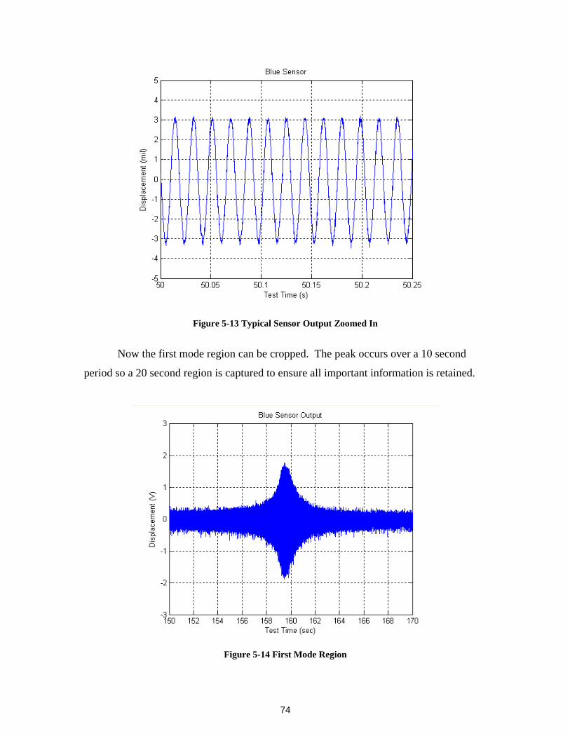
74
Figure 5-13 Typical Sensor Output Zoomed In
Now the first mode region can be cropped. The peak occurs over a 10 second
period so a 20 second region is captured to ensure all important information is retained.
Figure 5-14 First Mode Region
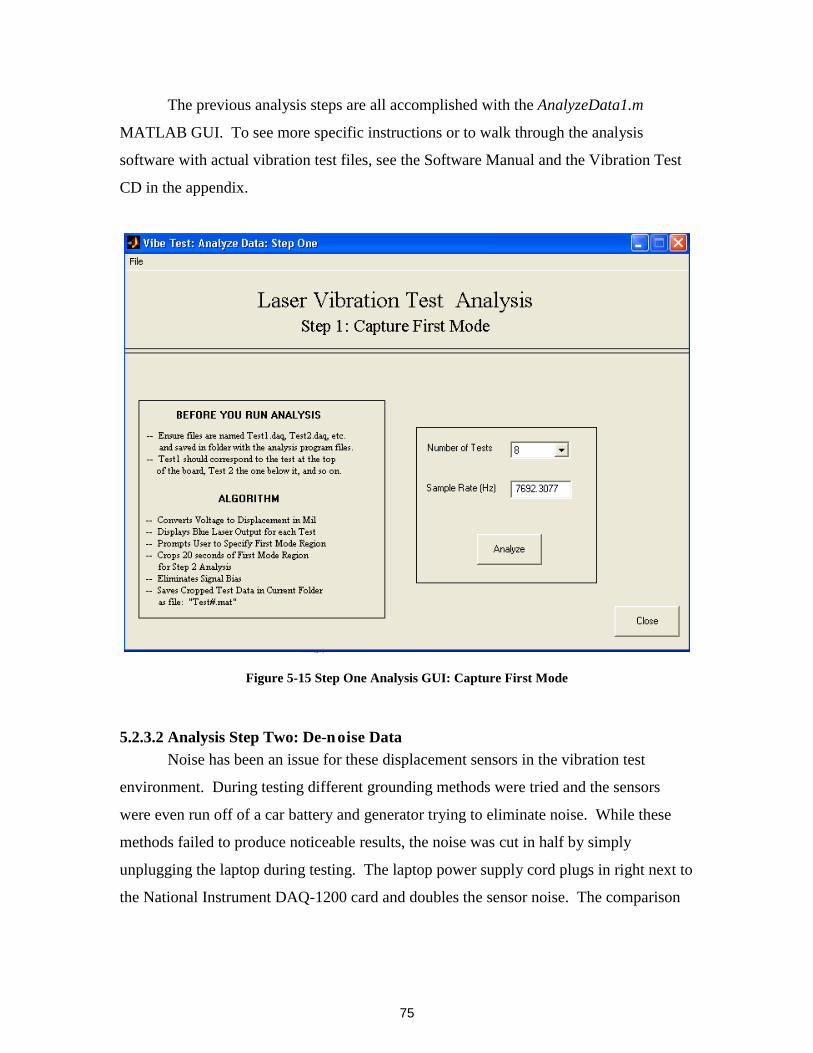
75
The previous analysis steps are all accomplished with the AnalyzeData1.m
MATLAB GUI. To see more specific instructions or to walk through the analysis
software with actual vibration test files, see the Software Manual and the Vibration Test
CD in the appendix.
Figure 5-15 Step One Analysis GUI: Capture First Mode
5.2.3.2 Analysis Step Two: De-noise DataNoise has been an issue for these displacement sensors in the vibration test
environment. During testing different grounding methods were tried and the sensors
were even run off of a car battery and generator trying to eliminate noise. While these
methods failed to produce noticeable results, the noise was cut in half by simply
unplugging the laptop during testing. The laptop power supply cord plugs in right next to
the National Instrument DAQ-1200 card and doubles the sensor noise. The comparison

76
of noise bands for the laptop plugged in versus running it off its battery can be seen
below. The noise band is cut from ±0.4 mil to ±0.2 mil.
According to the National Instruments online support page, when the DC voltage
is compared on both ends of the laptop power supply with respect to a solid reference,
there is a 60 Hz voltage pattern with a high peak-to-peak voltage that causes an unstable
analog input ground (AIGND), and therefore produces a noisy signal.
The LK-11 sensor specifications report that the sensor should have an output
resolution of 0.007 mil. It can be seen that even the noise band with the laptop running
off of its battery is greatly reducing the measuring resolution lower boundary.
Displacements below 0.2 mils are lost in the noise band and cannot be seen.
The noise is masking the first mode region so before the frequency content of the
data can be found; a de-noising technique had to be devised. An FFT was run on the 20
second first mode region to quickly identify the frequency components within the data so
filtering methods could be developed.

77
Figure 5-16 First Mode Region Power Spectral Density Plot: FFT
The largest peak occurs at 60 Hz indicating electrical noise is a large component
of the overall signal noise. The second highest peak is a wider band showing the
electronics board passing through its first natural frequency – this is what needs to be
isolated. The other substantial peaks occur in the higher frequency ranges. Two
techniques were used to isolate the first natural frequency peak: a simple band pass filter
and a more complex wavelet de-noising method.
5.2.3.2.1 Band Pass FilterA band pass filter was designed to capture the first mode frequency components
and discard the noise components. A band pass filter keeping everything between 525Hz
and 850 Hz was built. See figure on next page for filter algorithm and parameters. The
red shows the FFT of the 20 seconds of first mode data captured by a sensor and the blue
is the band pass filter that was designed. It can be seen that the filter would keep only the
first mode peak and hopefully discard the noise.
60HzElectrical Noise
Electronics Board1st Natural Frequency
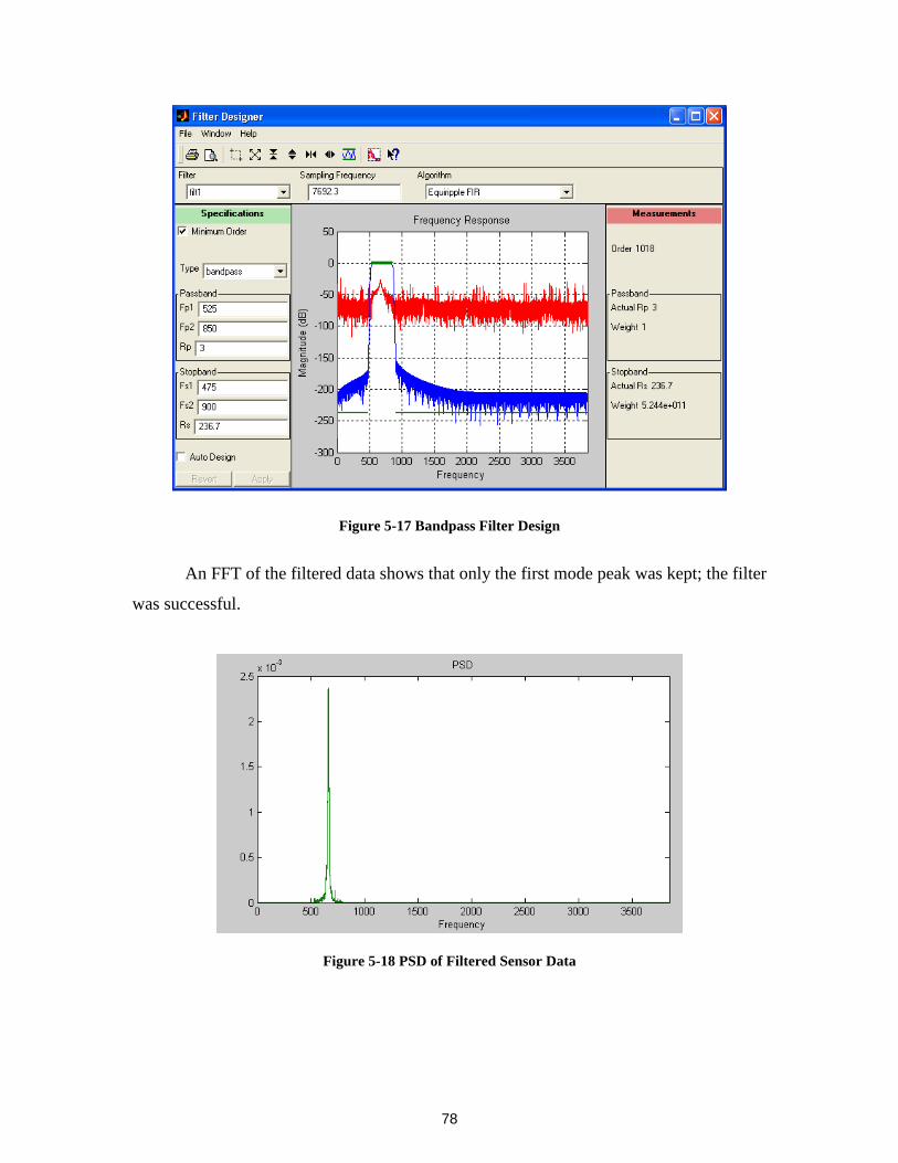
78
Figure 5-17 Bandpass Filter Design
An FFT of the filtered data shows that only the first mode peak was kept; the filter
was successful.
Figure 5-18 PSD of Filtered Sensor Data

79
The original data compared with the filtered time data shows that the filter caused
a slight delay and ripple effects in the data.
Figure 5-19 Original vs Filtered Sensor Data
5.2.3.2.2 Wavelet De-NoisingThe second method for de-noising involves splitting the displacement signal into
levels using a wavelet and removing those levels that contain noise components in them.
The Wavelet 1-D GUI in MATLAB was used to graphically explore how the different
wavelets broke up the displacement data into levels. The dmey was the only wavelet that
captured the first mode sinusoidal displacement in one level and the noise components in
the other levels. The dmey wavelet is a discrete approximation of a Meyer wavelet.
Because this wavelet separated the noise components from the sinusoidal displacements
of the resonating board, the dmey wavelet was chosen. To view a typical dmey wavelet
decomposition of the first mode region, see Figure 5-20.

80
Figure 5-20 DMEY Wavelet Decomposition of Modal Region
All of the details coefficients for the 12 levels were discarded except for d3 since
this level captured the true modal displacements. The signal was then reconstructed with
level 3 detail coefficients to output the de-noised data.

81
Figure 5-21 Original vs De-Noised Sensor Data
The dmey wavelet de-noising techniques look like they have de-noised the first
mode region quite well. There is no delay or rippling effects like the filtered data. To
ensure that all of the noise components of the PSD were eliminated and that the modal
region was kept, a FFT was run on the de-noised data. See figure below.
Figure 5-22 PSD of De-Noised Data
The FFT shows that the wavelet de-noising method was also successful in
eliminating the noise components and retaining the first mode.

82
5.2.3.2.3 Method Comparison: Filtering vs. Wavelet De-Noising
The plot below shows the original sensor output, filtered results, and de-noised
results.
Figure 5-23 Original, Filtered, and Denoised Comparison
The wavelet de-noising results used a more complex method to eliminate noise
and proved to produce better results. Since the method was chosen by visually inspecting
different wavelets and choosing the one that captured the mode the best without real
knowledge of wavelet techniques, it is interesting to see that the de-noising method
provided a smoother and more accurate representation of the original modal
displacements peak. The DMEY wavelet de-noising method was chosen for the process
used in step two of the analysis software.
Figure 5-24 Step Two Analysis GUI: De-noise
Filtered
Original andDe-Noised

83
5.2.3.3 Analysis Step Three: Find FrequenciesTo accurately represent the displacement of the electronics board during its first
mode, it is necessary to pick the amplitude and frequency content out of the time data
instead of relying on the vibration table sweep rate of 2 oct/min. To accomplish this, an
algorithm was written that determined the zero crossings of the sinusoidal displacement
data, and averaged the frequency output over a specified number of periods to smooth the
data and found the max positive displacement within each set of averaged cycles.
5.2.3.3.1 Zero Crossing Algorithm
The zero crossing algorithm uses a simple relationship to quickly process the data
and identify the zero crossings (ZC’s).
MATLAB Code:
y=denoised_data;
ZC_indice=find(([0 y] < 0) & ([y 0] > 0) | ([0 y] > 0) & ([y 0] < 0));
The above code finds where there is a sign change between the current
displacement value and the subsequent displacement value. The results of this algorithm
on the sensor output can be viewed in Figure 5-25.
Figure 5-25 Zero Crossing Algorithm Results

84
5.2.3.3.2 Interpolation and AveragingThe zero crossing algorithm can detect points closer to the zero axis if the data is
interpolated. Since the time between zero crossings will be used to indicate half-cycle
time for the frequency calculation, it is important that they are as accurate as possible.
For example, interpolating the data with a scale of two would double the data’s sample
rate and thus double the number of data points describing the output. The more times, the
data is interpolated, the better the results from the zero crossing algorithm. The
algorithm results after linearly interpolating the data with a sampling rate 15 times
smaller than the original data’s sample rate, can be viewed in Figure 5-26.
Figure 5-26 Zero Crossings with Linear Interpolation of Data
It can be seen that the zero crossings are now identifying points closer to zero
which will result in a more accurate frequency calculation.
5.2.3.3.3 Find Frequencies
After the data has been interpolated, the time between zero crossings is used to
calculate frequency. The more cycle times that are averaged, the smoother the frequency
output but the less data points there will be describing the first mode. The maximum
positive displacement is saved along with the averaged frequency value for each set of
cycles. The find frequency algorithm results are shown in Figure 5-27 on the next page.

85
Figure 5-27 Find Frequency Algorithm Results
The zero crossing and find frequency algorithms are used in the Step Three: Find
Frequencies of Mode GUI. The program allows the user to change the interpolation scale
and the number of cycles that will be averaged. The output is a file containing the
frequency and displacement values for each sensor.
Figure 5-28 Step Three Analysis GUI: Find Frequencies of Mode

86
5.2.3.3.4 Find Frequency Results: Original vs. De-noisedNow that a find frequency function exists to determine the frequencies of the
sensor’s output, a step back is going to be taken to look at how well the algorithm worked
on the de-noised data (output from Step Two) versus the original data (output from Step
One). This will help evaluate the importance of de-noising the data. See the plot below.
Figure 5-29 Find Frequency Algorithm Results: Original vs. De-noised Data
It can be seen that the de-noising worked extremely well in eliminating the 60 Hz
noise so the mode could be accurately captured. The original data yields barely readable
results.
5.2.3.4 Analysis Step Four: Clea n Modal DataThe frequency data from step three of the analysis has to be cleaned so that a
single displacement value exists for each frequency. To do this, the data is run through a
clean mode algorithm that deletes redundant frequency values so the remaining
displacement data is a valid function. Then the data is fit with a polynomial function

87
where discrete frequency and displacement data can then be found. See below to view
the results of cleaning and polyfitting the data.
Figure 5-30 Original vs. Cleaned Modal Displacement
Figure 5-31 Polynomial Fit of Cleaned Modal Displacement
The step four MATLAB GUI was written to step the user through the cleaning
and polyfitting steps. It is a tedious task to play with the polynomial degree and range to
find the best fit for the data but it is important to the accuracy of determining the first
mode of the board. The user visually determines the best range and degree for the fit.
The GUI can be seen on the next page.
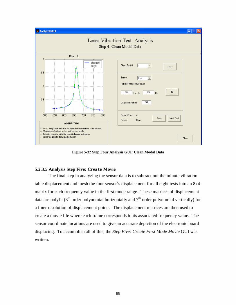
88
Figure 5-32 Step Four Analysis GUI: Clean Modal Data
5.2.3.5 Analysis Step Five: Crea te MovieThe final step in analyzing the sensor data is to subtract out the minute vibration
table displacement and mesh the four sensor’s displacement for all eight tests into an 8x4
matrix for each frequency value in the first mode range. These matrices of displacement
data are polyfit (3rd order polynomial horizontally and 7th order polynomial vertically) for
a finer resolution of displacement points. The displacement matrices are then used to
create a movie file where each frame corresponds to its associated frequency value. The
sensor coordinate locations are used to give an accurate depiction of the electronic board
displacing. To accomplish all of this, the Step Five: Create First Mode Movie GUI was
written.

89
Figure 5-33 Step Five Analysis GUI: Create First Mode Movie
In this GUI, the user can define the frequency range for the movie, the frames per
second, quality, compression used, and the movie name. The output is a movie file in
.avi format. The frequency recording with the greatest board displacement is the first
natural frequency.
The next page displays the final first mode results from the two tests that were
performed. The first test showed the first natural frequency at 659Hz with a 1.827mil
maximum displacement in the center of the board. The second test showed the first
natural frequency at 662 Hz with 1.827mil displacement in the center of the board. This
output proves that the system will provide repeatable results.

90
Figure 5-34 Test One First Mode Results
Figure 5-35 Test Two First Mode Results
The maximum displacement for each frequency over the first mode range can be
seen in Figure 5-36.
TEST 1: 1.827mils @ 662 Hz
TEST 1: 1.827mils @ 659 Hz

91
Figure 5-36 Laser Grid Results: Maximum Displacement
The only difference between the tests that should be noted is the labeling dot as
seen in Figure 3-3 was left on from the area scaling tests during Laser Test 1 but it was
removed for Laser Test 2. A discussion of these results and how they compare with
accelerometer testing will be explored in the next chapter.

92
[THIS PAGE INTENTIONALLY LEFT BLANK]

93
Chapter 6 System Performa nceThe laser vibration measurement and analysis system showed repeatable results
for the bare frame electronic board testing. The next step is to see how these
displacement and frequency results compare with accelerometer grid tests, as well as, the
center mounted accelerometer output. These comparisons will be discussed within this
chapter and will be used in setting the system specifications.
6.1 Accelerometer Grid ComparisonThe output from a 3x3 grid of accelerometers for the same electronic board used
in the laser tests and tested under the same vibration profile will be used to judge the
accuracy of the laser system. In order to reduce the mass loading effects, pico-sized
accelerometers made by Endevco were used; each is 0.14 grams in mass. Four tests were
performed using 3 accelerometers for each test. One accelerometer was kept in the center
of the board as a control. The other two were moved around the board creating a 3x3
grid. See the figures on the next page for the accelerometer locations and results.
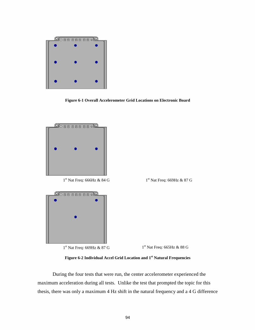
94
Figure 6-1 Overall Accelerometer Grid Locations on Electronic Board
Figure 6-2 Individual Accel Grid Location and 1st Natural Frequencies
During the four tests that were run, the center accelerometer experienced the
maximum acceleration during all tests. Unlike the test that prompted the topic for this
thesis, there was only a maximum 4 Hz shift in the natural frequency and a 4 G difference
1st Nat Freq: 669Hz & 87 G
1st Nat Freq: 669Hz & 87 G
1st Nat Freq: 666Hz & 84 G
1st Nat Freq: 665Hz & 88 G

95
in response amplitude. This illustrates that even using the 0.14g accelerometers on the
board, will result in a slight output difference from test to test and needs to be kept in
mind when comparing the laser results. While the accelerometer output is being used as
the real electronic board output, in actuality, the lasers could be capturing the real output
and the accelerometers could be giving output with slight mass loading effects [14].
The accelerometer data used the 3x3 accelerometer output to create a meshed
board response. The center control accelerometer was averaged for all four tests worth of
data. Then the meshed output was fit with a second order polynomial in both the vertical
and horizontal directions to display the 3-D acceleration and displacement of the board.
The first natural frequency occurred at 668Hz with a response amplitude or 83.9 G’s.
This correlates to a maximum first mode displacement of 1.84 mil at 668 Hz.
Figure 6-3 Accel Grid 3-D Output: Acceleration and Displacement at First Natural Frequency
Unlike the Laser Vibration System, the accelerometer data can display the
displacement for the entire 20-2000Hz test, not just areas where the displacement is over
the noise band. The maximum displacement of the board during the entire test is shown
in Figure 6-4.
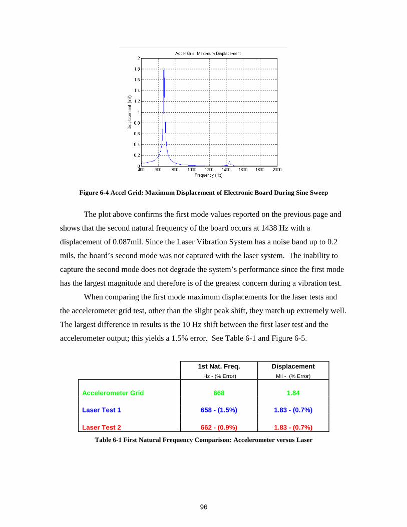
96
Figure 6-4 Accel Grid: Maximum Displacement of Electronic Board During Sine Sweep
The plot above confirms the first mode values reported on the previous page and
shows that the second natural frequency of the board occurs at 1438 Hz with a
displacement of 0.087mil. Since the Laser Vibration System has a noise band up to 0.2
mils, the board’s second mode was not captured with the laser system. The inability to
capture the second mode does not degrade the system’s performance since the first mode
has the largest magnitude and therefore is of the greatest concern during a vibration test.
When comparing the first mode maximum displacements for the laser tests and
the accelerometer grid test, other than the slight peak shift, they match up extremely well.
The largest difference in results is the 10 Hz shift between the first laser test and the
accelerometer output; this yields a 1.5% error. See Table 6-1 and Figure 6-5.
1st Nat. Freq. Displacement Hz - (% Error) Mil - (% Error)
Accelerometer Grid 668 1.84 Laser Test 1 658 - (1.5%) 1.83 - (0.7%) Laser Test 2 662 - (0.9%) 1.83 - (0.7%)
Table 6-1 First Natural Frequency Comparison: Accelerometer versus Laser

97
Figure 6-5 First Mode Max Displacement Comparison: Laser versus Accelerometer Output
6.2 Center Accelerometer ComparisonThe first mode of the electronic board, as seen in Figure 6-3, is where the center
of the board has the greatest displacement. During each laser vibration test, a test control
accelerometer captured the board’s response close to this center location. The average
center accelerometer output for all eight laser test position runs versus the 8x4 laser grid
results can be seen below.7
Laser Test 1 Laser Test 2Nat. Freq Disp Nat. Freq Disp
Hz mil Hz milCenter Accel 659 1.77 664 1.82Laser 658 1.83 662 1.83
Table 6-2 Center Accelerometer vs. Laser Results
7 The laser test results approximate the board’s center displacement through fitting the 8x4 grid withpolynomial functions. The laser did not actually record the center of the board except in sensor selectiontesting seen in Chapter 4.

98
6.3 Laser Versus Accelerometer DiscussionThe center accelerometer output is closer to the natural frequency and dynamic
response than the comparison between the accelerometer grid and laser grid results. This
shows that the lasers are doing a better job at identifying the natural frequency of the
board than the accelerometer grid results are illustrating. There is a possibility the
accelerometer grid testing is changing the dynamics of the board through the addition of
the two accelerometer’s mass. Earlier in Figure 6-2, it was shown that three pico-sized
accelerometers moved around on the face of the board caused the natural frequency at the
center accelerometer to range between 665 Hz and 669Hz.
Intuitively, the addition of the accelerometers should lower the natural frequency
since mass is being added to the board. This assumption is based on the equation below.
Equation 6-1 mk=ω
where ω is the natural frequency, k is the spring constant, and m is the mass of the object.
Another more interesting relation between mass-loading and its effect on the
natural frequency of a board was seen during an experimental study describing the effects
of masses and their location on the natural frequencies of plates. It was found that the
fundamental frequency increases as the mass moves away from the center of the plate
[14]. This could explain why the natural frequency for the accelerometer grid testing is
greater than the laser test results. Also, the 3 Hz difference among the laser testing can
be explained by the removal of the labeling dot from the center of the board for the
second laser test – reduction in mass would cause an increase in natural frequency. It is
also possible this slight first mode variation is unrelated and is just the slight error in
accelerometer output between tests.
6.4 Hardware Vibration
The hardware mounted accelerometer is located on the sensor cross bar next to
the sensor heads. It is measuring the amount of vibration seen by the laser displacement
sensors in the horizontal direction to ensure false displacements are not being recorded.

99
The prototype system with the one LK-11 attached saw displacements of concern at
200Hz while with the heavier LC-2440 sensor attached, the displacements were minimal.
Along with the four sensors, weights were added to the top of the cross bar to help reduce
the amplitude of the 200Hz peak. See figure below for accelerometer location on the
final system.
Figure 6-6 Hardware Accelerometer Location
The hardware accelerometer output can be viewed below. The center
accelerometer is also plotted to show the magnitude of board displacement seen by the
lasers.
Figure 6-7 Magnitude of Hardware Vibration
HardwareAccelerometer

100
At 200 Hz the hardware experiences a sizable resonance. Hardware Test 1
accelerometer output (positioned so sensors are capturing the top of the electronic board)
has a peak at 200 Hz and 0.12 mil, while the hardware accelerometer output for Test 8
(sensors capturing the base of the board) has a displacement of 0.3 mil around 200 Hz.
This difference exists because as the cross bar and sensors are moving down the vertical
rails, there is a longer moment arm on the sensor fixturing system.
While the 200Hz peak is of concern for the system performance, since the
hardware introduced negligible displacement levels in the first mode region, it is not a
concern for the specific test completed in this thesis. However, for laser tests examining
object responses in the 200Hz region, there should be hardware modification or a close
watch of the hardware’s displacement during testing.
6.5 System SpecificationsDrawing on the results presented, system specifications can now be determined.
The original ideal specification were defined in Table 2-3 to determine how well the
system is performing compared with the desired performance set in the preliminary
design stage.
Metric Imp Units Ideal Final Sample Rate 5 Hz 10k 7.8k Deflection of Object 5 mil ±4 ± 39 Resolution 5 mil 0.05 0.008 mil Cost 4 $US <25k <25k
Full Field 4 in2 450 (12 in diam) 4 points
Time to Assemble andDisassemble 3 min. 30 30
Measurement Area 3 in2 See Full Field
4 discrete pointshorizontally with
1cm verticalresolution
Test Time 3 min. 3 30
Table 6-3 System Specifications: Preliminary versus Final

101
Overall, the system outperforms the ideal specifications. The system’s final
specifications prove it to be a versatile system that can be used for a wide range of
vibration tests. The ±39 mil measurement range at a sample rate of 7.8 kHz with
0.008mil resolution is outstanding. Also, the displacements for any test object surface
type can be read with this system. The only drawback is the noise band that masks all the
displacements below 0.2mil. The amazing part of this system is that it is integrating four
off the shelf displacement sensors into a non-contact measurement and analysis system
that has cost less than $25k. The closest non-contact measurement system is a bulky
single point laser vibrometer sensor from Polytec PI that retails for $25k, while a
scanning system starts at 160k.
The entire system has a hassle free setup with a time to assemble and disassemble
at less than 30 minutes. Most of that time spent zeroing the sensor position and waiting
for the lasers to warm up for the most stable measurements. The 30 minute test time is
based on the amount of time it takes to capture the 8x4 grid of displacement during the
sine sweep along with the time it takes to raise or lower the cross bar.
Two of the three most important preliminary specifications, were almost 10x
better than expected. Overall this system has proven a viable alternative to
accelerometers and because it does not physically touch the test object, it will provide
more accurate vibration test results.

102
[THIS PAGE INTENTIONALLY LEFT BLANK]

103
Chapter 7 Conclusions and RecommendationsPrompted by accelerometers mass loading an electronic board during vibration
testing, the goal of this thesis was to design a non-contact vibration measurement and
analysis system to capture the un-altered dynamic performance of an electronic board
during vibration testing.
A product development process was used to guide the design process. First,
customer needs were identified to help set preliminary specifications. After non-contact
measurement methods were explored, three concepts were proposed: holographic
interferometry, area scaling, and displacement sensor grid. Concept testing, preliminary
analysis and comparison ratings determined that the displacement sensor grid concept
would be the best method for this system.
A prototype hardware and software package was built to test the two laser
displacement sensors under consideration. The Keyence LK-11 laser displacement sensor
was determined to be the better sensor over the Keyence LC-2440 since it was more

104
compact, cheaper per unit, less sensitive to noise, and could read the displacement of any
surface type. Also, the prototype hardware and software system were evaluated during
the sensor selection vibration testing improvements. This feedback was used to design
the final non-contact system.
Four Keyence LK-11 laser displacement sensors were incorporated into the final
system. The setup arranges the four sensors side by side setting the minimum distance
between the laser points at 0.7 inches. The vertical movement mechanism allows the row
of sensors to be vertically positioned in 1cm increments up or down the face of the
electronics board. For the testing conducted in this thesis, the system allowed for an 8x4
displacement grid of the electronic board to be captured.
The final software was written in MATLAB to acquire and analyze the board’s
displacement during the 20-2000Hz sine sweep. A five step analysis program starts by
cropping the first natural frequency region from the sensor’s displacement data. This first
mode displacement data is de-noised using wavelet de-noising techniques. Then, the
frequencies and maximum positive displacements are determined using the data’s
sinusoidal zero crossing times. Finally, all of the first mode displacements are meshed
into an 8x4 grid where they are fit with a 3rd order polynomial in the horizontal direction
and a 7th order polynomial in the vertical direction to output a movie depicting the
electronic board displacing through its first mode region.
7.1 Conclusions
This thesis has shown laser displacement sensors are a low cost and highly
accurate way to perform non-contact vibration measurements. Overall, the final system
outperformed the specifications set earlier in the preliminary design stage. While it does
not produce full field modal displacement output like holographic interferometry
techniques, it can record 4 points horizontally with 0.7 inch resolution and numerous
points vertically at 1cm resolution with the current hardware setup.
Combined with the data acquisitions and analysis software, the laser displacement
system found the natural frequency and maximum displacement amplitudes within 1.5%
and 0.7% accuracy, respectively, when compared with previous acceleration grid results.
The system has a maximum sample rate of 7.8kHz. It can record displacements up to

105
±1mm, and it can read the displacement of objects with any surface type or material. The
sensors have a 0.2µm or 0.8 micro-inch resolution.
The only drawback to these sensors is that displacements below 2 mils were
indistinguishable because of a sensor noise band. Work was done to reduce this noise,
but the only successful action to note is that running the laptop off of its battery instead of
the power supply cord during testing reduced the noise band from 4 mils to 2 mils.
The four sensors are integrated into a clean, easy to setup hardware/software
package. It takes less than 15 minutes to fully configure to test setup, however, the
sensors need 30 minutes warm up time to provide a stable output. The software package
provides easy to use MATLAB GUI’s to acquire and analyze the output. While it was
specifically written for outputting a movie file using the 8x4 displacement grid of the
electronic board’s first mode, it can be easily adapted for other vibration test cases.
7.2 Recommendations
While this system proves using laser displacement sensors a viable method for
non-contact vibration measurement, further work can be done to develop a more accurate
and versatile non-contact test measurement and analysis system.
Currently, the sensor mount setup is relying on the test object being a flat surface.
A sensor mount providing individual sensor adjustment towards or away from the test
specimen would ensure that sensors did not impact a test object with an uneven surface.
Individual adjustment would allow for electronic board component analysis to be easily
performed and it would introduce a more accurate way to null the sensor’s position.
The idea of clamping to the side rails of the vibration table to isolate the sensors
was a fast, low cost method that proved successful. However, it was a tedious task to
ensure the sensors were in the correct position since the tops of the rails are not perfectly
smooth. If a mount were drilled to the inside or top of the vibration table side rails, it
would provide a more accurate way of dangling the sensors 1 cm in front of the test
object.
Since the test system is capturing displacements on the order of a thousandth of an
inch, a more rigid system might reduce laser point position error and transferred vibration
levels seen in the hardware mounting the sensors. The hardware was adequate for the

106
level of accuracy needed in capturing an 8x4 grid of board displacements, however, the
weight of the sensor themselves probably caused slight off center twist that changed the
laser point position and might be the reason why the four sensors could not be positioned
perfectly planar with the board.
Although, the software was written for the specific electronic board test, it does
reveal the analysis methodology that can be applied to any test case. The software should
be expanded, however, to allow for multiple test configurations.
Finally, the system performance and accuracy were established through
comparison with electronic board accelerometer output. Different test profiles should be
run to validate the performance of this system in more than the one test profile presented
in this thesis. The 2-mil noise band should be further investigated to increase the lower
displacement limit capabilities of the system.
With the numerous benefits of non-contact instrumentation, test facilities should
incorporate this low cost and versatile method of non-contact measurement into their
testing practices.
107
References
[1] Figliola, Richard S. and Beasley, Donald E., “Measurement of Acceleration and Vibration,”Theory and Design for Mechanical Measurement, 3rd ed., John Wiley & Sons, New York,2000, pp. 482-488.
[2] Whitham, Eleri M. and Griffin, Michael J., “Measuring Vibration on Soft Seats” Society ofAutomotive Engineers, Inc. SAE paper 770253, 1977.
[3] Ulrich, Karl T. and Eppinger, Steven D., Product Design and Development, 2nd ed., IrwinMcGraw-Hill, Boston, 2000.
[4] Steinberg, Dave S., “Electronic Equipment for Airplanes and Missiles,” Vibration Analysisfor Electronic Equipment, 3rd ed., John Wiley & Sons, New York, 2000.
[5] Sensors: Vision and Measurement 2002-2003. Keyence, 2003.
[6] Welsby, Scott D., “Capacitive and Inductive Noncontact Measurement” SensorsMag.com,March 2003, URL: http://www.sensorsmag.com [cited 29 April 2004].
[7] URL: http://www.micro-epsilon.com/ [cited 29 April 2004].
[8] Hariharan, Parameswaran, Basics of Holography, Cambridge University Press, 2002.
[9] Fein, Howard, “Holographic Interferometry: Nondestructive Tool,” The IndustrialPhysicist, Vol. 3, No. 3, Sep. 1997, pp. 37-39.
[10] Inman, Daniel J., “Vibration Testing and Experimental Modal Analysis,” EngineeringVibration, 2nd ed., Prentice Hall, 2001.
[11] Stanbridge, A.B. and Ewins, D.J., “Modal Testing Using a Scanning Laser DopplerVibrometer,” Mechanical Systems and Signal Processing, Vol. 13, No. 2, March 1999, pp.255-270.
[12] “Image Processing Toolbox: Image Analysis: Analyzing and Enhancing Images: SobelMethod,” MATLAB 6.5.1, Release 13, software Help file.
[13] “How Do I Calculate my Camera Sensor Resolution and Lens Focal Length?” NationalInstruments Knowledge Base [online database], URL: http://www.ni.com [cited 19 April2004].
[14] Low, K.H., “An Equivalent-Center-Weight Factor Method for Predicting FundamentalFrequencies of Plates Carrying Multiple Masses from Experimental Test Data,” Journal ofSound and Vibration, 1993, pp. 123-139.

108
[THIS PAGE INTENTIONALLY LEFT BLANK]

NON-CONTACT VIBRATION SYSTEMNon-Contact Vibration Measurement Hardware Manual
Hardware Manual

N O N - C O N T A C T V I B R A T I O N M E A S U R E M E N T H A R D W A R E S E T U P
110
Hardware SetupThis Hardware Manual will help you properly setup and configure the non-contact vibration
measurement system for vibration testing. For more information on the test setup and results, please seeChapter 5and 6 of this thesis.
4, LK-11DisplacementSensors
Weights
THK Linear Bearing- Discrete PositionMechanism
Vise RailClamp
Cross Bar
Sensor Mounts
DRO

N O N - C O N T A C T V I B R A T I O N M E A S U R E M E N T H A R D W A R E S E T U P
111
Subassembly OneLeft Vise and Vertical
Key Parts1. Vise Clamp2. L-Bracket3. Vertical4. THK Linear Bearing Rail5. 2-Hole Bracket6. ¼ - inch Pin7. THK Linear Bearing Truck8. Bronze Cross Bar End9. 1/8-inch Nut/Bolt Bearing Stopper (2)10. 3/8-inch Slot Bolt/Washer/Nut
6
1
2
7
5
43
8
9 10
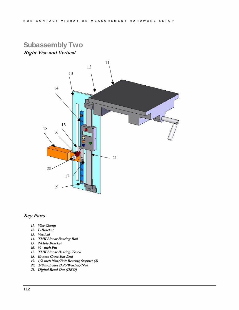
N O N - C O N T A C T V I B R A T I O N M E A S U R E M E N T H A R D W A R E S E T U P
112
Subassembly TwoRight Vise and Vertical
Key Parts11. Vise Clamp12. L-Bracket13. Vertical14. THK Linear Bearing Rail15. 2-Hole Bracket16. ¼ - inch Pin17. THK Linear Bearing Truck18. Bronze Cross Bar End19. 1/8 inch Nut/Bolt Bearing Stopper (2)20. 3/8-inch Slot Bolt/Washer/Nut21. Digital Read Out (DRO)
1112
13
14
15
21
16
17
18
19
20

N O N - C O N T A C T V I B R A T I O N M E A S U R E M E N T H A R D W A R E S E T U P
113
Subassembly ThreeCrossbar and Sensors
Key Parts22. Cross Bar23. Weights24. Keyence LK-11 Laser Displacement Sensor (4)25. Mount Plate Right26. Mount Plate Left27. Mount Slot Bracket (2)
22
24
23
2527
26

N O N - C O N T A C T V I B R A T I O N M E A S U R E M E N T H A R D W A R E S E T U P
114
Assembly StepsStep One: Assemble Hardware
• Clamp Subassembly One and Two vises to vibration table side rails
• Slide Sensors/Crossbar Assembly onto Bronze Bar Ends
`
• Insert ¼ inch diameter bolts, washers, and nuts to secure the cross bar to the two bronze barends. Leave bolts loose so sensors can be positioned with respect to electronic board.
• Mount electronic board to vibration table.
• Center Lasers with respect to the electronic board by using the slots on the cross bar. Ensurethe fixture will not hit the sensors. There is a very small clearance.
• Tighten ¼” bolts to secure cross bar to bronze bar ends.
Preassembled andHanging on VibrationTable Rails

N O N - C O N T A C T V I B R A T I O N M E A S U R E M E N T H A R D W A R E S E T U P
115
Assembly StepsStep Two: Power Laser Sensors
• Connect sensors to controllers with extension cables. Ensure the sensor number matches thecontroller number.
• Tune both DC Power Supply Channels to + 24 V.
• Ensure Lasers are Connected to controllers
• Ensure Laser keys are in the OFF position
• Hook up Ground
• Hook up PS 1 and PS 2 wires to power laser controllers with 24V DC each.

A C Q U I S I T I O N A N D A N A L Y S I S S O F T W A R E
116
Assembly StepsStep Three: Hook up Data Acquisitions Card and Laptop
• Connect colored output wires from the controller unit to the NI DAQ Card. Followthe wiring schematic on previous page.
� Yellow � 2
� Blue � 3
� Green � 4
� Red � 5
� Ground � 9
• Turn ON laptop
• Ensure NI DAQ 6.9.3 is installed
• Open MATLAB
• Open the directory where the software has been installed
• Type “AcquireData” in the Command window
Refer to Software Manual for further information

A C Q U I S I T I O N A N D A N A L Y S I S S O F T W A R E
` 117
Assembly StepsStep Four: Laser Settings
• Open Front Covers on each laser controller
• Set the sensors to 128µs sample cycle (Fs=7812.5Hz)
• Set the Mode to Normal
• DIP Switches
� Alarm � Hold
� Key Protect � Free
� Response � High
• Turn Laser Keys to ON
• Hold down Zero/Reset button for 5 seconds to ensure the sensors are NOT zeroed
• Turn Lasers to ON Position
• Please see Keyence LK-3100 Series Instruction Manual for more detailed informationabout operating the lasers and specific modes.
IMPORTANT
1. Laser Keys must be in the OFF position BEFORE the Power is turned OFF
2. Lasers CANNOT be Disconnected from Controllers until the Lasers are OFF and thePower is OFF

A C Q U I S I T I O N A N D A N A L Y S I S S O F T W A R E
` 118
Assembly StepsStep Five: Adjust Laser Position for Test
• Center the laser output around 0 Volts by positioning the sensors 1 cm from theelectronic board.
� With vises loose, and lasers ON, move the lasers about 1 cm away from theelectronic board until the lights on the back of the sensors are all green or afew are green and a few are solid orange indicating the sensors are in a validmeasurement distance.
� NOTE: If the sensor lights are flashing orange, they are either out of range orstuck between the green and orange range which can cause false readings.
• Preview the sensor output by viewing the voltage output plots with the MATLABprogram AcquireData.
• Zero the Sensor’s Vertical Position
� Move the sensors so the laser points are on the top of the electronic board.
� Move the Digital Read Out (DRO) down until it is resting on the bracket.
� Hit Zero on the DRO box.
Indicator LightsShown All Green
Zero

A C Q U I S I T I O N A N D A N A L Y S I S S O F T W A R E
` 119
• Now Move the sensors into the first data collection position. See below for how touse the vertical movement mechanism to lower the cross bar exactly 1 cm at a time.
• Tighten the Slot Bolts on each vertical
• Push the DRO down until it stops on the bracket.
• Record the DRO measurement value for the location of the first row of laserpoints. The DRO will indicate the distance from the top of the board so every laserposition will now be known.
• Tighten all of the bolts to secure the cross bar in place.
• Please see Software Manual for software setup and functions.
You are now ready to test!
Pin in top Bracket holePin in bottom Bracket hole and lowerbore on the Rail. Sensors are nowpositioned 1cm lower

A C Q U I S I T I O N A N D A N A L Y S I S S O F T W A R E
` 120
IMPORTANT TESTING NOTES:
• Sensors may need to be readjusted (moved towards/away from the board) when the vibrationtable is turned on.
• Software: Remember to Save each test run before you start taking data for another test.
• TURN Lasers to the OFF position BEFORE you remove Power!
• Sensors MUST be in the OFF position with Power Removed BEFORE they are disconnectedfrom the controllers.
NON-CONTACT VIBRATION SYSTEMData Acquisitions and Analysis Software Manual
Software Manual

A C Q U I S I T I O N A N D A N A L Y S I S S O F T W A R E
122
Data AcquisitionThis program uses the MATLAB Data Acquisition Toolbox to acquire the voltage output from the
Keyence LK-11 displacement sensors through a National Instruments NI-DAQ 1200 card. Two files exist foruse: the AcquireData.m is for testing with the Non-Contact Laser Vibration System and a demo file,AcquireData_SoundCard.m, was written to allow users who do not have the NI-DAQ card to see how thesoftware works by simply capturing the data off their computer’s sound card.
The AcquireData.m (Laser Vibration Test 2.0) is used to capture the output of the four displacementsensors during a test. A sensor coloring scheme has been used in this program so that the sensors are neverconfused. The Red sensor captures the displacement data on the left of the board, then the Green is to itsright, the Blue is next, and then the Magenta. The Red Sensor displacement is the first column of data withinthe .daq file even though it is routed to the Channel 5 slot on the NI-DAQ 1200 board. Red=data(:,1),Green=data(:,2), Blue=data(:,3), Mag=data(:,4). This is just how the NI-DAQ 1200 reads the channels.Remember to save the data acquired after each test run.
Data Acquisitions Demo
• Insert Laser Vibration CD
• Save files from CD to a directory on your computer.
• Open MATLAB
• Change the current directory to the directory where you saved the files.
• To run the sound card demo, type in the MATLAB prompt window:Acquiredata_soundcard
o Alternatively, type Acquirdata to run the vibration test program that acquires datafrom the NI-DAQ Card.
The Laser Vibration Test 2.0 window should open.
• Press the Start button and you will see the sound card data in the plot windows.

A C Q U I S I T I O N A N D A N A L Y S I S S O F T W A R E
123
Plot windows with sound card output.
Program Options
Vertical Location: User can view where the lasers are capturing the data. This value is promptedwhen you go to save the data so location information can be retained.
Sample Rate: User can change this value to anything. In AcquireData.m, the program will ensure it isa NI-DAQ-1200 sample rate and if not, it will change it to the closest one.
Duration: The User can specify the Duration for Vibe Test to capture the data. During a vibrationtest this value should be set on inf so the user can just stop the acquisition when the test is complete.
Start/Stop: Starts or Stops data acquisition from sound card or NI-DAQ 1200 card.
Setup Help: Provides a diagram of how the Laser Vibration System should be setup.
Close: Closes Laser Vibration Test 2.0.
File → Save: Saves the acquired data as a .daq file
File → Send To → Workspace: Sends the acquired data and Fs (sample rate) information to theMATLAB Workspace.
File → Send To → SPTool: Sends acquired data to the Signal Processing Tool
File → Send To → Figure: Plots the acquired data as a time plot and an FFT plot

A C Q U I S I T I O N A N D A N A L Y S I S S O F T W A R E
124
Data AnalysisThe analysis programs use MATLAB in a five step series of m-files to analyze the test data and
output an .avi file showing the electronics board first mode displacement. The Laser Vibration System cancapture the displacement of the board with eight tests, one every 1cm down the board with Test1.daqcorresponding to the top test, Test2.daq to the second from the test, and so on until Test8.daq is at thebottom of the board.
NOTE: The Test files from the second 20-2000Hz sine sweep test reported in this thesis are located onthe CD and will allow the Analysis software to be used. This will provide a better understanding of theanalysis steps taken to convert the raw displacement sensor voltage into a 3D movie file of the electronicboard displacing through its first mode.
Step One: Capture First ModeAnalyzedata1.m
• Type AnalyzeData1 to open the first step of the analysis
The following window should open:
• Set the Number of Tests to 8
• Set the Sample Rate to 7692.3077 Hz
• Press Analyze

A C Q U I S I T I O N A N D A N A L Y S I S S O F T W A R E
125
A figure will appear with the specified Test data plotted with the axis zoomed into the first moderegion.
Then a CropModal dialog box will appear asking what 20 second time range the first mode shouldbe cropped around. Try to capture the displacement peak in the center of the 20 second rangeand do not to crop an area where noise has caused a hiccup in the data. The mode will differfrom the noise in that the mode should have x-axis symmetry and the noise will not.
• Press OK
The program will run through all of the tests, and save the cropped modal regions as Test#.mat inthe current directory, where # will refer to the test number for the data.
Program Options
Number of Tests: User can pick how many tests will be loaded to have their first modecaptured.
Sample Rate: User must specify the sample rate at which the data was acquired.
Close: This will close the program.

A C Q U I S I T I O N A N D A N A L Y S I S S O F T W A R E
126
Step Two: DenoiseAnalyzedata2.m
This analysis step de-noises the data by splitting the displacement signal into 12 levels using theDMEY wavelet. Then the displacement signal is recreated with the only details component, d3, thatcaptures the sinusoidal resonant displacement and very little noise.
• Type AnalyzeData2 to open the first step of the analysis
The following window should open:
• Set the Number of Tests to 8
• Press DeNoise
A figure window will appear showing each of the 8 tests with their original displacement dataand the denoised output (yellow).
The De-noised data is automatically saved as Denoised#.mat in the current directory.

A C Q U I S I T I O N A N D A N A L Y S I S S O F T W A R E
127
Step Three: Find Frequencies of ModeAnalyzedata3.m
This analysis step reads in Denoise#.mat displacement and time data for the specified number oftests and outputs displacement and frequency data as FreqData#.mat. The frequency content isdetermined by the zero crossing time within the sinusoidal data. The more the data is interpolated thebetter the frequency output but the longer this program will take. The frequencies can be averaged over aspecified number of cycles to get smoother output.
• Type AnalyzeData3 to open the first step of the analysis
The following window should open:
• Set the Number of Tests to 8
• Set Sample Rate to 7692.3077 Hz
• Set Interpolate Data to 15 x
• Set Average to 15 cycles
• Press FindFreq

A C Q U I S I T I O N A N D A N A L Y S I S S O F T W A R E
128
Program Options
Number of Tests: User can pick how many tests will be loaded.
Sample Rate: User must specify the sample rate at which the data was acquired.
Interpolate Data: User can specify the number of times the data is interpolated. The greater thenumber the more data points are added between the existing data points.
Average: The Frequency found for each sinusoidal period can be averaged over a User selectednumber of periods to provide smoother output.
Close: This will close the program.

A C Q U I S I T I O N A N D A N A L Y S I S S O F T W A R E
129
Step Four: Clean Modal DataAnalyzedata4.m
This analysis step reads in FreqData#.mat for the specified test file, cleans it of its redundant x-values, and fits a polynomial function to the data so that there is one displacement value for eachfrequency. If the data cleaning does not work correctly, more data cropping will have to be performed.The polyfit data is saved as PolyData#color.mat.
• Type AnalyzeData4 to open the first step of the analysis
The following window should open:
• Set Clean Test # to 1
• Press Clean

A C Q U I S I T I O N A N D A N A L Y S I S S O F T W A R E
130
The following figure opens displaying the original data with the cleaned data (yellow). The red,green, and blue sensor data was cleaned nicely but the magenta data had too much noise that theclean_mode algorithm failed. The data for the magenta data will have to be recropped.
The CropModal2 dialog box opens asking if the data needs to be recropped for better cleaningresults.
• Press Yes
Now another dialog box asks which sensors need to be recropped.
• Check the Magenta box
• Click OK

A C Q U I S I T I O N A N D A N A L Y S I S S O F T W A R E
131
Now the CropModalData GUI opens displaying the Magenta Sensor Data. This GUI willdelete the data below the specified amount.
• Enter 0.09 mil
• Press Preview Crop
The cropped data should just capture the hill of displacements and not the noise beneath it. Inthis case, deleting the data below 0.09 mils left a little noise, so let’s crop at a little greaterdisplacement.
• Enter 0.095 mil
• Press Preview Crop
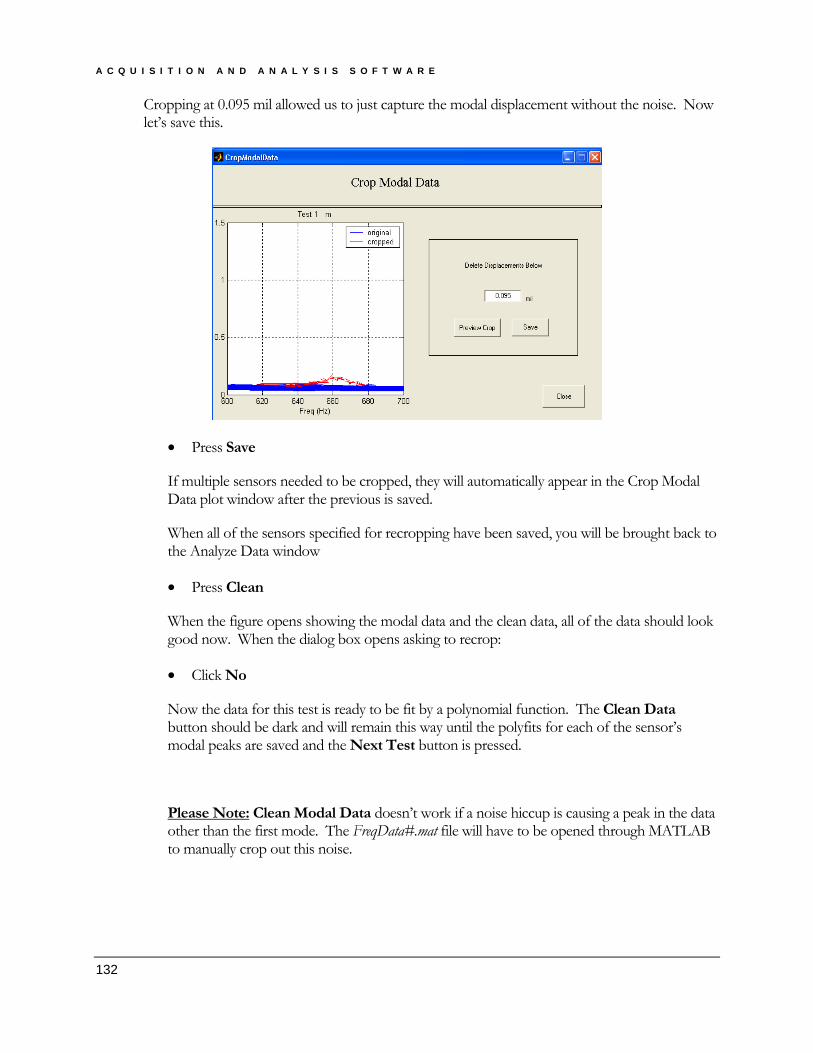
A C Q U I S I T I O N A N D A N A L Y S I S S O F T W A R E
132
Cropping at 0.095 mil allowed us to just capture the modal displacement without the noise. Nowlet’s save this.
• Press Save
If multiple sensors needed to be cropped, they will automatically appear in the Crop ModalData plot window after the previous is saved.
When all of the sensors specified for recropping have been saved, you will be brought back tothe Analyze Data window
• Press Clean
When the figure opens showing the modal data and the clean data, all of the data should lookgood now. When the dialog box opens asking to recrop:
• Click No
Now the data for this test is ready to be fit by a polynomial function. The Clean Databutton should be dark and will remain this way until the polyfits for each of the sensor’smodal peaks are saved and the Next Test button is pressed.
Please Note: Clean Modal Data doesn’t work if a noise hiccup is causing a peak in the dataother than the first mode. The FreqData#.mat file will have to be opened through MATLABto manually crop out this noise.

A C Q U I S I T I O N A N D A N A L Y S I S S O F T W A R E
133
• Select the Red Sensor
• Change the Frequency Range to 620 Hz to 700 Hz
• Change the Degree of PolyFit to 10
This polynomial fit does a good job of fitting the data but the degree could be increased to helpcapture the peak better. Play with the range and degree until you like the way it looks. A smallfrequency range now will result in a small frequency range for the movie file of the electronicsboard displacing through the first mode region.

A C Q U I S I T I O N A N D A N A L Y S I S S O F T W A R E
134
If the degree is too high for the frequency range, the polynomial will look like the plot below.Decrease the degree or just reduce the range so this can be avoided.
A better poly fit:
Once you like the polyfit,
• Press Save
• Repeat poly fit for each sensor
• Press Next Test to start the cleaning and data fitting steps over for subsequent tests.

A C Q U I S I T I O N A N D A N A L Y S I S S O F T W A R E
135
Step Five: Create MovieAnalyzedata5.m
This analysis step reads in the sensor displacements output from Analyzedata4 and creates amovie file of the electronics board.
• Type AnalyzeData5
The following window should appear:
• Set Number of Test to 8
• Set Compression to Indeo5
• Set Quality to 100
• Set Frames per Second to 25
• Set Frequency Range to 650 to 680 Hz
• Press Make Movie

A C Q U I S I T I O N A N D A N A L Y S I S S O F T W A R E
136
A figure window will open to display each frame of the movie file as the displacement data fromeach sensor and test are meshed at each frequency in the range specified.
The movie will be automatically saved in the local directory with the Movie Name specified.
To View Movie
Open Windows Media Player or Quicktime and select the movie file from the directory it wassaved in.
PROBLEMS VIEWING MOVIE
Install the Indeo 5 Codecs from CD by following the directions in the ReadMe.txt file located inthe IndeoVideo5 folder.
Top Related