


Languages
Pages
Legal

Design and Analysis ofExperiments
David YanezDepartment of BiostatisticsUniversity of Washington

Outline Basic Ideas Definitions Structures of an Experimental Design
Design StructureTreatment Structure
The Three R’s of Experimental Design Examples
Basic Ideas
Questions:
What is the scientific question? What are the sources of variation? How many treatments are to be studied? What are the experimental units? How does the experimenter apply the treatments to
the available experimental units and then observe theresponses?
Can the resulting design be analyzed or can thedesired comparisons be made?
Homilies
“To call in the statistician after the experiment isdone may be no more than asking him toperform a postmortem examination…
… he may be able to say what the experimentdied of.''
R.A. Fisher, Indian Statistical Congress,Sankhya, ca 1938
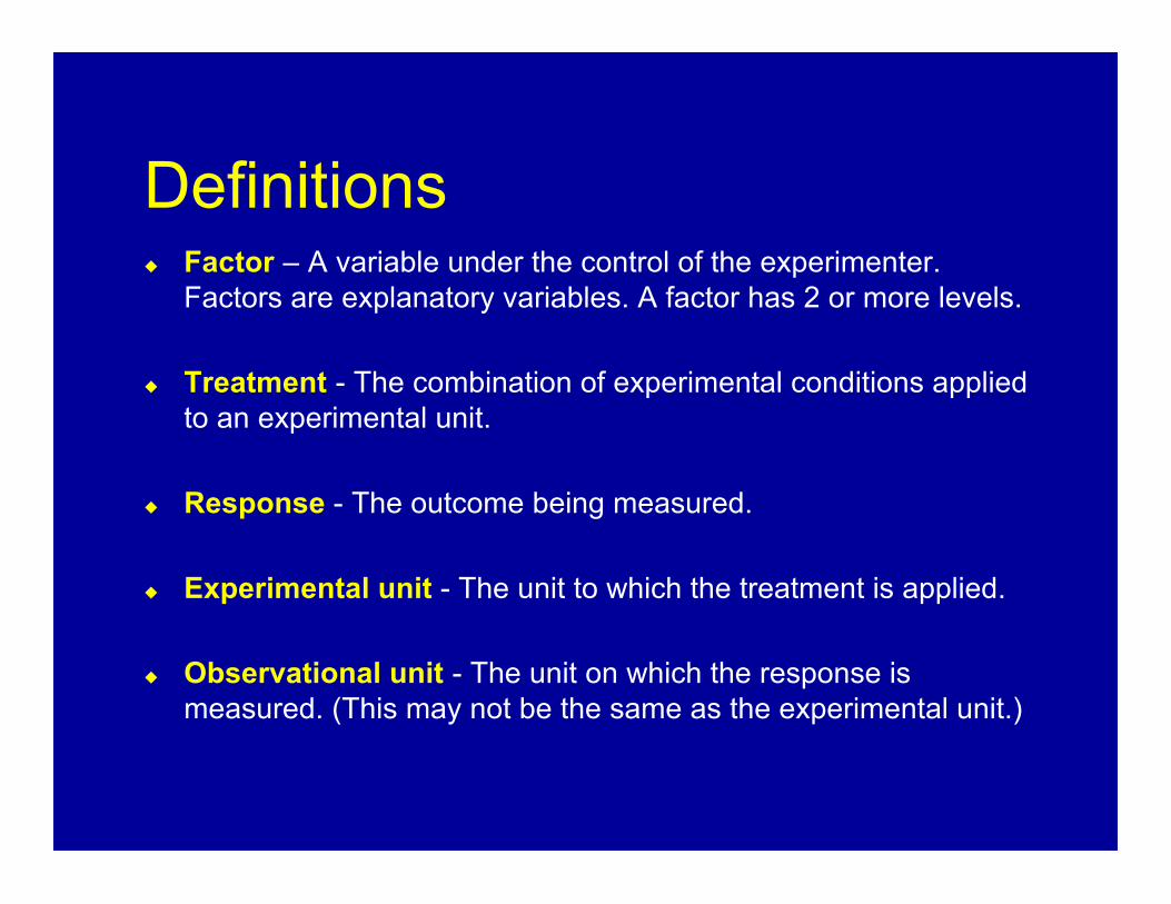
Definitions Factor – A variable under the control of the experimenter.
Factors are explanatory variables. A factor has 2 or more levels.
Treatment - The combination of experimental conditions appliedto an experimental unit.
Response - The outcome being measured.
Experimental unit - The unit to which the treatment is applied.
Observational unit - The unit on which the response ismeasured. (This may not be the same as the experimental unit.)

Experimental DesignStructures Design Structure
The grouping of the experimental units intohomogeneous blocksE.g., twins, gender…
Why might this be important?To ensure a fair comparison when the number
of experimental units is “small”
Experimental DesignStructures
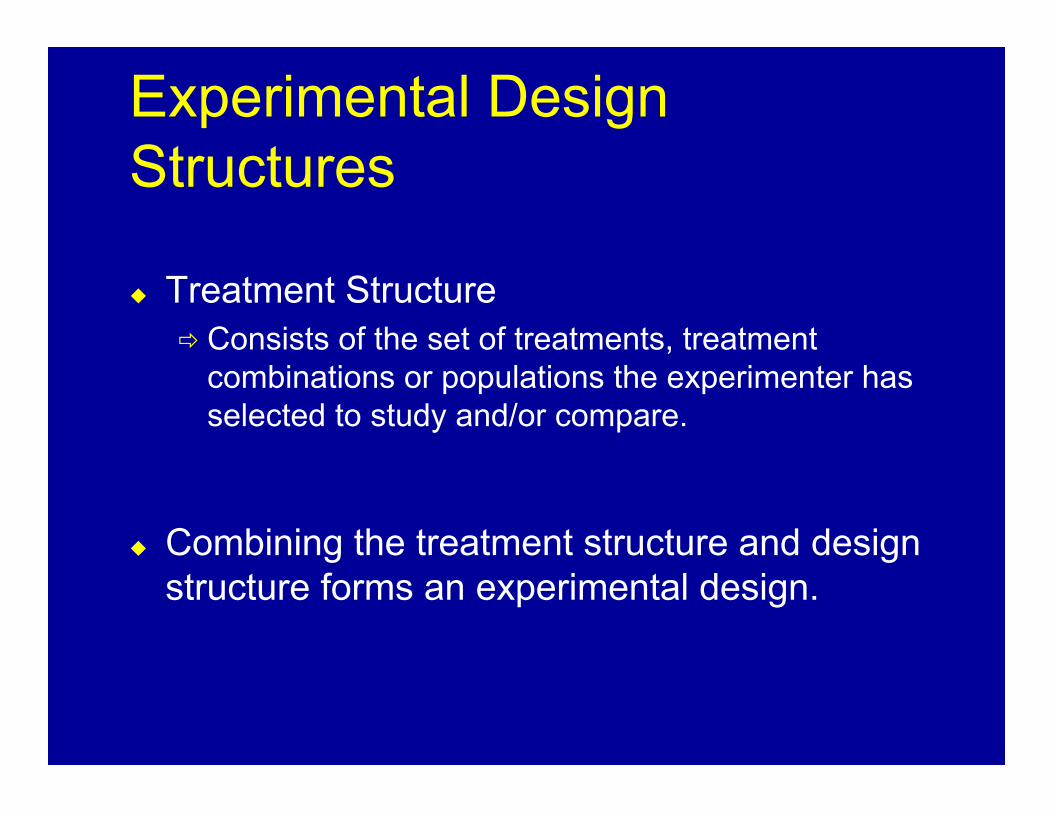
Treatment Structure Consists of the set of treatments, treatment
combinations or populations the experimenter hasselected to study and/or compare.
Combining the treatment structure and designstructure forms an experimental design.
The Three R’s of ExperimentalDesign
Randomization Replication Stratify (block)

The Three R’s (cont.)
Randomization – It is important to randomizebecause it averages out the effect of all other lurkingvariables - it doesn't remove their effects, but makes,on average, their effects equal in all groups.
Proper randomization is crucial Iron deficiency in rats experiment

The Three R’s (cont.) Replication – A replication is an independent
observation of a treatment. Two replications of atreatment must involve two experimental units.
Important to have replication to insure you have power todetect differences
Randomization helps to make fair or unbiased comparisons,but only in the sense of being fair or unbiased whenaveraged over a whole sequence of experiments.
Beware of pseudo-replication (sub-sampling) Pig myocardium experiment

The Three R’s (cont.)
Blocking – Experimental units are divided intosubsets (blocks) so that units within thesame block are more similar than units fromdifferent subsets or blocks.
If two units in the same block get differenttreatments, the treatments can be comparedmore precisely than if all the units in oneblock received one treatment, all in anotherreceived the second.
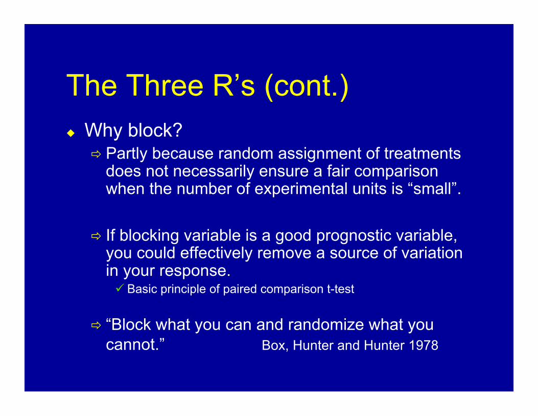
The Three R’s (cont.) Why block?
Partly because random assignment of treatmentsdoes not necessarily ensure a fair comparisonwhen the number of experimental units is “small”.
If blocking variable is a good prognostic variable,you could effectively remove a source of variationin your response. Basic principle of paired comparison t-test
“Block what you can and randomize what youcannot.” Box, Hunter and Hunter 1978

Examples Example 1 – An agricultural experimental station is going to test
two varieties of wheat. Each variety will be tested with two typesof fertilizers. Each combination will be applied to two plots ofland. The yield will be measured for each plot.
Treatment: Varieties of wheat and fertilizer types
Response: yield
Experimental unit: plots
Observational unit: plots
Examples (cont.)
Example 2 – Scientists want to study the effect of an anti-bacterialdrug in fish lungs. The drug is administered at 3 dose-levels (0, 20,and 40 mg/L). Each dose is administered to a large controlled tankthrough the filtration system. Each tank has 100 fish. At the end ofthe experiment, the fish are sacraficed, and the amount of bacteria ineach fish is measured.
Treatment: Dose levels of antibacterial drug
Response: Amount of bacteria
Experimental unit: Tanks
Observational unit: Fish
Examples (cont.) Example 3 – A study was conducted to examine the crop yield
for 3 varieties of corn, V, under 5 different fertilizers, F. A 15row field was available for the experiment. The experimenterfirst randomly assigned each of the 5 fertilizers to exactly 3rows.
Treatment: Fertilizer
Response: Yield
Experimental unit: Row
Observational unit: Row

Examples (cont.)
F3F5
F3F1
F2
F1
F5
F4
F5
F2
F5
F2
F4
F3
F1
Rows The treatment structure for F can bewritten as
Yik = µ + Fi + εik, i =1,…,5; k =1,2,3;where µ is the overall mean, Fi is the effect of fertilizer type i εik is a mean zero random error
term.
Examples (cont.) The experimenter also wants to study the 3 varieties of corn.
Suppose the experimenter randomly assigns the 3 varieties toexactly 5 rows.
Treatments: Corn varieties and fertilizers
Response: Yield
Experimental unit: Row
Observational unit: Row

Examples (cont.)
The model for F and V is Yijk = µ + Fi + Vj + (FV)ij+ εijk
where µ is the overall mean, Fi is the effect of fertilizer type i, Vj is the effect of variety j, (FV)ij is the fertilizer by variety
interaction, εijk is a mean zero random error term.
F3 F5F1 F2 F4
V3
V1
V2
Fertilizer Type
Variety
Examples (cont.) The experimenter does wish to investigate a fertilizer by
variety interaction. S/he decides to divide each of the 15 rows,r, into 3 subplots, then randomly assigns one of the 3 cornvarieties, V, to each of the subplots.
Treatment: Corn varieties
Response: Yield
Experimental unit: Subplot
Observational unit: Subplot
Examples (cont.)
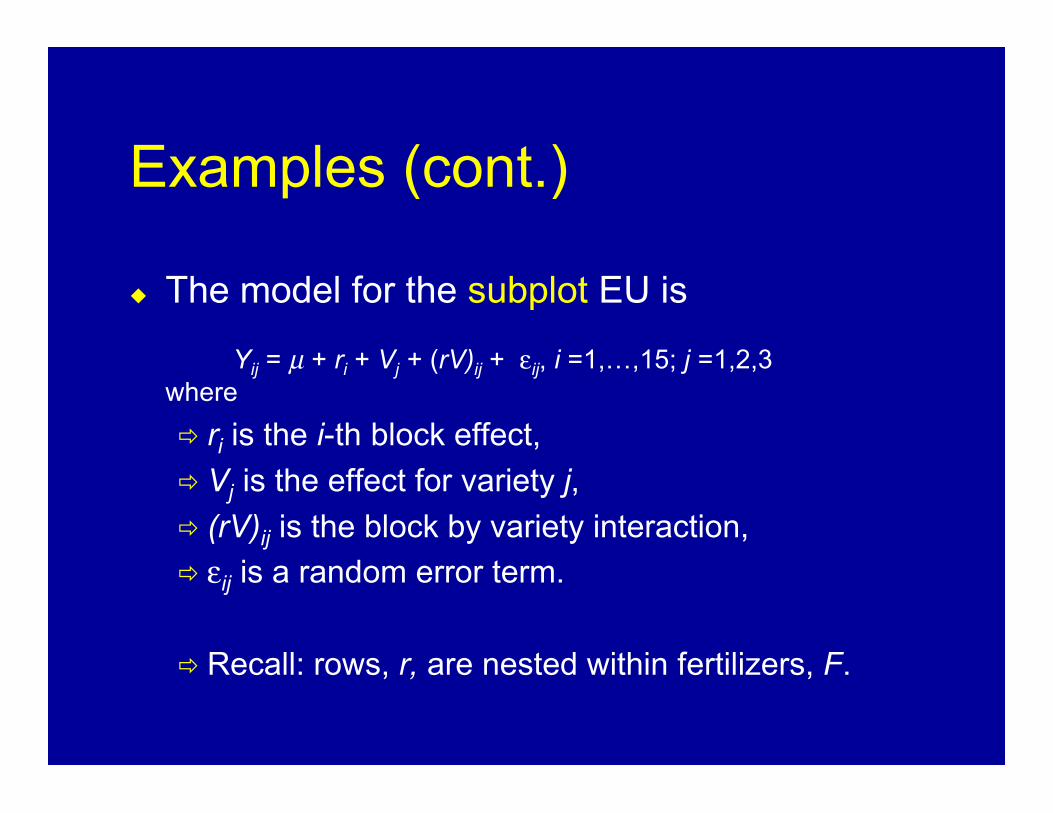
The model for the subplot EU is
Yij = µ + ri + Vj + (rV)ij + εij, i =1,…,15; j =1,2,3where
ri is the i-th block effect, Vj is the effect for variety j, (rV)ij is the block by variety interaction, εij is a random error term.
Recall: rows, r, are nested within fertilizers, F.

Examples – Split Plot Model
In the first design, rows were theEUs; the factors F and V werecompletely crossed.
In the split plot design, subplotsform one level of the EU. Therow is a (blocking) factor. Rowsare nested within fertilizers andcrossed with varieties.
F3 F5F1 F2 F4
V3
V1
V2
Fertilizer Type
Variety
1 2
F4
F1
F3
Rows
FF2
F5
3 4 5 6 7 158 9 …V1
V3
V2

Examples – Split Plot Model
Experimental Units – 2 levels 1. The EUs (rows) are (randomly) assigned one level of the
whole plot factor (e.g., fertilizer type F4). 2. EUs are then split into smaller EUs (subplots) and receive
all levels of the subplot factor (e.g., varieties V1, V2, V3).
Model: Yijk = µ + Fi + rk(i) } whole plot part + Vj + (FV)ij + εijk } sub plot part

Examples – Split Plot Model ANOVA Table
Source df E[MS]Between plot 14
Fertilizer, F 4 σε2 + 3σr
2 + 3*3 Σi Fi2/(5-1)
Row(F) 10 σε2 + 3σr
2
Within plot 30Variety, V 2 σε
2 + 3σvr2 + 3*5 Σj Vj
2/(3-1)V x F 8 σε
2 + 3σvr2 + 3 Σij (FV)ij
2/{(5-1)(3-1)}V x Row(F) 20 σε
2 + 3σvr2

Yijk = µ + Fi + rk (i ) +Vj + (FV )ij + !ijk
i = 1,..., p = 5 fertilizers each assigned to 3 rows
j = 1,...,q = 3 varieties assigned to the 3 subplots in each row
k = 1,...,r = 3 rows within each fertilizer
In fact, we need an extra random effects component for the random row x variety interaction:
Yijk = µ + Fi + rk (i ) +Vj + (FV )ij + (vr) jk (i ) + !ijk
where rk (i ) ! N(0," r
2), (rv) jk (i ) ! N(0," vr
2), !ijk ! N(0,"
!
2)
Source Df MS E(MS) Between plot pr-1 = 14 Fertilizer, F (p-1) = 4
1
p !1Yiii !Y( )
2
i, j ,k
" !"
2+ q! r
2+
qr
p #1Fi2
i$
Row(F) p(r-1) = 10
1
p(r !1)Yiik !Yiii( )
2
i, j ,k
" !"
2+ q!
r
2
Within plot pr(q-1) = 30 Variety, V q-1 = 2
1
q !1Y
i j i !Y( )2
i, j ,k
" !"
2+! vr
2+
pr
q #1Fi2
i=1
p
$
V x F (p-1)(q-1) = 8
1
(p !1)(q !1)Yij i !Yiii !Yi j i +Yiii( )
2
i, j ,k
" !"
2+! vr
2+
r
(p #1)(q #1)(FV )ij
2
i, j
p,q
$
V x Row(F) p(r-1)(q-1) =20
1
p(r !1)(q !1)Yijk !Yij i !Yiik +Yiii( )
2
i, j ,k
" !"
2+!
vr
2

Split Plot Model
What’s so special about the split plot model? Allows one to model correlated data in a univariate model. Relatively easy to fit. Model assumes
Balance design, exchangeable correlation for the whole plot EU.

Repeated Measures Model Example 4 – An experimenter is interested in vigilance performance.
S/he desires to evaluate the relative effectiveness of two modes ofsignal presentation: an auditory signal and a visual signal . Thesecond treatment corresponding to four successive two-hourmonitoring periods. Eight graduate students were randomly assignedto one of the two modes of presentation. Response latency scoreswere recorded on each participant at each successive 2-hour period.
Whole plot factor: Signal presentation
Subplot factor: Time (in 2-hour increments)
Problems?
Repeated Measures Model
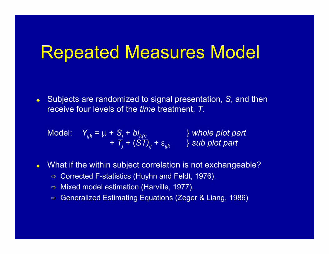
Subjects are randomized to signal presentation, S, and thenreceive four levels of the time treatment, T.
Model: Yijk = µ + Si + blk(i) } whole plot part + Tj + (ST)ij + εijk } sub plot part
What if the within subject correlation is not exchangeable? Corrected F-statistics (Huyhn and Feldt, 1976). Mixed model estimation (Harville, 1977). Generalized Estimating Equations (Zeger & Liang, 1986)
Top Related