


Languages
Pages
Legal

Constructing an Evaluation Function for Playing Backgammon
A N D E R S S J Ö Q V I S T a n d A N D R É S T E N L U N D
Bachelor of Science Thesis Stockholm, Sweden 2011

Constructing an Evaluation Function for Playing Backgammon
A N D E R S S J Ö Q V I S T a n d A N D R É S T E N L U N D
Bachelor’s Thesis in Computer Science (15 ECTS credits) at the School of Computer Science and Engineering Royal Institute of Technology year 2011 Supervisor at CSC was Johan Boye Examiner was Mads Dam URL: www.csc.kth.se/utbildning/kandidatexjobb/datateknik/2011/ sjoqvist_anders_OCH_stenlund_andre_K11069.pdf Kungliga tekniska högskolan Skolan för datavetenskap och kommunikation KTH CSC 100 44 Stockholm URL: www.kth.se/csc

Abstract
In this project we describe a few variations of the game backgammon. We explain different algorithms,
used to play backgammon and other similar games, and develop our own rule engine and a set of players.
By developing an evaluation function for playing board games, we aim to find out if it’s possible to
construct a simple computerized player that outperforms other players, and which properties such a
player should have. The player programs that we have developed are very primitive, but there are
distinct tendencies revealing which players dominate the others. The winning player’s only strategy is
to hit the opponent’s lone checkers, while protecting its own.
Sammanfattning
I denna uppsats beskriver vi några varianter av spelet backgammon. Vi går igenom olika algoritmer
som anvands for att spela backgammon och andra liknande spel, och utvecklar vår egen regelmotor och
en uppsattning spelare. Vi vill skapa en evalueringsfunktion for att spela bradspel så att vi ska kunna
ta reda på om det går att konstruera en enkel datorspelare som vinner over andra spelare, och vilka
egenskaper en sådan spelare ska ha. Spelarprogrammen som vi utvecklat ar mycket primitiva, men det
ar andå tydligt vilka spelare som tenderar att dominiera andra. Den vinnande spelaren har som sin
enda strategi att slå ut motståndarens ensamma pjaser, medan den skyddar sina egna.

Contents Contents
Contents
1 Introduction . . . . . . . . . . . . . . . . . . . . . . . . . . . . . . . . . . . . . . . . . . . . . . . 3
1.1 Statement of collaboration . . . . . . . . . . . . . . . . . . . . . . . . . . . . . . . . . . . . . 3
2 Problem statement . . . . . . . . . . . . . . . . . . . . . . . . . . . . . . . . . . . . . . . . . . . . 4
3 Playing backgammon . . . . . . . . . . . . . . . . . . . . . . . . . . . . . . . . . . . . . . . . . . 4
3.1 Terminology and basic rules . . . . . . . . . . . . . . . . . . . . . . . . . . . . . . . . . . . . 4
3.2 Rules of classic backgammon . . . . . . . . . . . . . . . . . . . . . . . . . . . . . . . . . . . 4
3.3 Rules of Greek backgammon . . . . . . . . . . . . . . . . . . . . . . . . . . . . . . . . . . . 5
3.3.1 Portes . . . . . . . . . . . . . . . . . . . . . . . . . . . . . . . . . . . . . . . . . . . . 5
3.3.2 Fevga . . . . . . . . . . . . . . . . . . . . . . . . . . . . . . . . . . . . . . . . . . . . . 5
3.3.3 Plakoto . . . . . . . . . . . . . . . . . . . . . . . . . . . . . . . . . . . . . . . . . . . . 6
4 Computer algorithms . . . . . . . . . . . . . . . . . . . . . . . . . . . . . . . . . . . . . . . . . . 6
4.1 Minimax . . . . . . . . . . . . . . . . . . . . . . . . . . . . . . . . . . . . . . . . . . . . . . . 7
4.2 Expectimax . . . . . . . . . . . . . . . . . . . . . . . . . . . . . . . . . . . . . . . . . . . . . . 7
4.3 Alpha-beta pruning . . . . . . . . . . . . . . . . . . . . . . . . . . . . . . . . . . . . . . . . . 8
4.4 *-Minimax . . . . . . . . . . . . . . . . . . . . . . . . . . . . . . . . . . . . . . . . . . . . . . 8
4.5 Knowledge-based evaluation . . . . . . . . . . . . . . . . . . . . . . . . . . . . . . . . . . . 8
4.6 Neural networks . . . . . . . . . . . . . . . . . . . . . . . . . . . . . . . . . . . . . . . . . . 8
5 Constructing our own evaluation function . . . . . . . . . . . . . . . . . . . . . . . . . . . . . . 9
5.1 Research process . . . . . . . . . . . . . . . . . . . . . . . . . . . . . . . . . . . . . . . . . . 9
5.2 Choice of game rules . . . . . . . . . . . . . . . . . . . . . . . . . . . . . . . . . . . . . . . . 9
5.3 Choice of algorithm . . . . . . . . . . . . . . . . . . . . . . . . . . . . . . . . . . . . . . . . . 10
5.4 Rule engine . . . . . . . . . . . . . . . . . . . . . . . . . . . . . . . . . . . . . . . . . . . . . 10
5.5 AI players . . . . . . . . . . . . . . . . . . . . . . . . . . . . . . . . . . . . . . . . . . . . . . 11
5.6 Automated test framework . . . . . . . . . . . . . . . . . . . . . . . . . . . . . . . . . . . . 13
6 Results . . . . . . . . . . . . . . . . . . . . . . . . . . . . . . . . . . . . . . . . . . . . . . . . . . . 13
7 Conclusions . . . . . . . . . . . . . . . . . . . . . . . . . . . . . . . . . . . . . . . . . . . . . . . . 14
8 Further research . . . . . . . . . . . . . . . . . . . . . . . . . . . . . . . . . . . . . . . . . . . . . 14
9 Acknowledgements . . . . . . . . . . . . . . . . . . . . . . . . . . . . . . . . . . . . . . . . . . . 15
References . . . . . . . . . . . . . . . . . . . . . . . . . . . . . . . . . . . . . . . . . . . . . . . . . . . 15
2


1 Introduction 1.1 Statement of collaboration
1 Introduction
Artificial intelligence for computerized gameplay
has been studied for a long time, but not until re-
cently has the topic gained publicity. [6, p. xix]
While some of the algorithms have few appli-
cations outside the domain of human-imitating
gameplaying opponents, they still have quite a
few things to teach us. Firstly, in their algorith-
mic forms they can improve our understanding
of probability, tactics and consequences of pre-
vious decision-making. Secondly, they serve as
measurements of the development in the com-
puter industry, as they are one the easiest compre-
hensible ways of comparing human intelligence
with computational thoroughness (especially in
the well-known matches between computers and
human world champions). Thirdly, the bene-
fits of the development of efficient gaming oppo-
nents shouldn’t be underestimated, as they pro-
vide recreation as well as sharpening of our logical
and tactical abilities, which is often benefitial in
other situations in our lives.
The game of backgammon is particularly interest-
ing, and is one of the most studied problems. [7]
It’s a two-player zero-sum game with a chance ele-
ment. Since we might experience “bad luck” with
the dice throws, the chance element makes it im-
possible to develop a strategy that is guaranteed
to perform well in at least 50 % of the games in the
short run, as even a novice player can beat a skilled
one thanks to luck (but note that this won’t happen
in the long run, when “the luck runs out”). Devel-
opment of new software for playing backgammon
can improve the availability of games for different
platforms, as well as promote further research of
the topic. Backgammon is also theoretically inter-
esting; if we decide that the problem we want to
solve is to find the true probability of winning from
a given game state when both players are rational,
it turns out that we don’t know whether the prob-
lem is in P. [3] That makes it unlikely that we will
find a simple algorithm for solving it anytime soon,
and requires us to create methods for optimizing
our guesses.
In this project, we intend to present a few dif-
ferent games played on the the same backgam-
mon board and explain our reasons for choosing
a certain set of rules. Furthermore, we will in-
troduce algorithms, frequently used when imple-
menting backgammon artificial intelligence (AI)
players. Lastly, we’ll describe our own experi-
ments for constructing an evaluation function, the
conclusions we drew and discuss possibilities for
future research.
1.1 Statement of collaboration
This thesis has been written entirely by Anders
Sjoqvist and Andre Stenlund. It’s our firm belief
that every task must be assigned to exactly one in-
dividual, or else it might be overlooked. Accord-
ing to this principle, Andre was assigned the main
responsibility of coding the rule engine and game-
playing software, as well as running the tests. An-
ders, on the other hand, was responsible for finding
appropriate literature, deciding about algorithms
and writing the report. The division of responsibil-
ities also roughly represents how the work was di-
vided, although we made sure that we both agreed
on everything. In addition, some tasks were done
jointly, as exemplified by the separate rule engine
written by Anders and parts of the literature search
which was made by Andre.
3
3.2 Rules of classic backgammon 3 Playing backgammon
2 Problem statement
We want to use Alpha-beta pruning and Expecti-
max to find an efficient backgammon AI evaluation
function, in order to increase our own understand-
ing, summarize some important algorithms and
draw conclusions about the behavior of a few sim-
ple tactics. Preferably, these conclusions should be
able to help game developers or enable future re-
search. Specifically, this is the question we want to
answer:
“Is it possible to construct an evaluation
function that, using simple and humanly
comprehensible rules, with statistical sig-
nificance can outperform other evalua-
tion functions in backgammon?”
3 Playing backgammon
The information in this section is available
from various sources, but we recommend using
Backgammon Galore for reference. [1] They also
have some information about how backgammon
programs work.
We will hereby explain the rules of a few games.
The rules are provided for completeness, to ensure
that a reader who has already played backgammon
understands the rules in the same way that we do.
It’s out of the scope of this thesis to try to teach a
beginner how to play, and although the rules that
we have implemented are also described here, they
might be explained more intuitively elsewhere.
3.1 Terminology and basic rules
Backgammon is a two-player game, and the game
pieces (often divided into black and white) are
called checkers. A player initiates his turn by throw-
ing the two dice, which must be thrown together
and display an unambiguous result (i.e. if at least
one die lands on the floor or stops in a tilted posi-
tion, both dice must be thrown again). The check-
ers are then, if possible, moved around the board
and placed on some of the 24 points. The points are
located on both sides of the board, with 12 on each
side, and divided into groups of six by the verti-
cal bar. If a point is occupied by a single checker,
it’s called a blot. Depending on the variant of the
game, the blot might be hit by the opponent and
placed on the bar. The six final points along the
path of movement for one of the players is called
that player’s home board. If a player has a checker
on the bar, he must enter it into the opposing home
board before he can make any other move. If there
are no possibilities to enter the checker, given the
numbers on the dice, the player must wait a turn.
Once all the checkers are gathered in the own home
board, the player may start bearing off the checkers.
3.2 Rules of classic backgammon
Figure 1 depicts the initial board setup in classic
backgammon. The game is played with two dice,
indicating the movement of the checkers. A dice
throw of {3, 5} means that two checkers may be
moved 3 and 5 points, respectively, or that one
checker may be moved twice, a total of 8 points
(but only in case a temporary stop on the 3rd or
5th point is legal, which is the case when at most
one of the opponent’s checkers is placed there). If
both dice show the same number, the player should
instead make four moves, if possible. As long as
there’s at least one possible move, the player is
forced to move. If there are different possibilities,
any is permitted.
In the setup in Figure 1, Black moves counter-
clockwise along increasing numbers from the
4

3 Playing backgammon 3.3 Rules of Greek backgammon
��������z�������-------------ZZZZZ
UVrst
klmno
pqrst
klmno
pqrst
PQRST
ZZZZZ
zzzzz
ZZZZZ
pqrst
PQRno
pqrst
klmno
pqrst
KLMNO
ZZZZZ
ZzzzzzzZzZzzzzzzZZZZZZ
edc10
jihgf
edcba
jihgf
edcba
JIHGF
ZZZZZ
zzzzz
ZZZZZ
edcba
jiHGF
edcba
jihgf
edcba
98765
ZZZZZ-------------
��������z�������Figure 1: Setup of classic backgammon
lower left corner to the upper left. The movement
of White is mirrored – from the upper left to the
lower left. The objective of the game is to move
all the checkers to the home board, so that they
can be borne off. The first player to bear off all the
checkers wins the game.
The strategy of the game is to build so-called
doors, a point with at least two checkers. Blots are
to be avoided if possible, as they can be hit by the
opponent and placed on the bar. In other words,
the doors both protect the checkers and prevent
the opponent from landing on that point. A player
may continue to move after a hit if there are any
moves left, in accordance with the numbers on the
dice. If there are checkers on the bar, they must
be entered into the game before any other moves
are allowed for that player. They are entered by
landing on a free point (or a point with a blot)
in the opponent’s home board, according to the
numbers on the dice.
Classic backgammon involes a doubling die, al-
lowing a player, about to roll, to propose that they
double the stakes. This forces the opponent to
choose between continuing with raised stakes or
ending the game and thereby losing the number of
points that the doubling die is currently display-
ing.
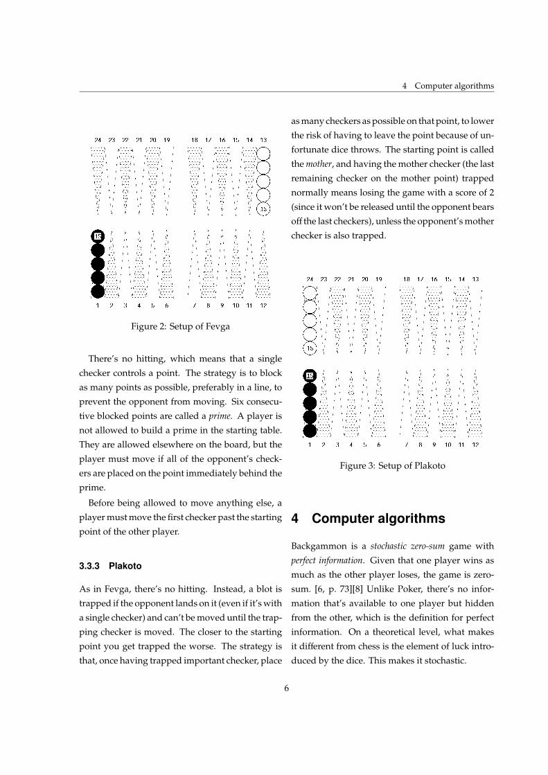
3.3 Rules of Greek backgammon
There are, of course, other variants of backgammon
than the classic one. We were also considering
the three Greek games of Portes (Πόρτες), Plakoto
(Πλακωτό) and Fevga (Φεύγα).
One difference from Western backgammon that
made us consider the Greek games, was that they
lack the doubling die, present in classic backgam-
mon. Instead, if a player manages to bear off all the
checkers before the opponent has borne off a single
one, the winning score will be 2 instead of 1. The
choice of game will be discussed and explained in
subsection 5.2 and suggestions concerning inclu-
sion of other games are mentioned in section 8.
The other difference in Greek backgammon is that
the winner of the opening roll rerolls for his first
turn.
3.3.1 Portes
Apart from the above-mentioned differences, the
game is the same as Western backgammon. The
initial setup is the same as the classic, shown in
Figure 1, and the name itself, Portes, refers to the
strategy of building doors.
3.3.2 Fevga
Fevga means escape, and has to do with the fact
that the players chase each other in the same
counter-clockwise direction on the board. This
setup, shown in Figure 2, is symmetrical along the
diagonal rather than the horizontal.
5
4 Computer algorithms
��������z�������-------------ZZZZZ
pqrst
klmno
pqrst
klmno
pqrst
klmno
ZZZZZ
zzzzz
ZZZZZ
pqrst
klmno
pqrst
klmno
pqrst
KLMNµ
ZZZZZ
ZzzzzzzZzZzzzzzzZZZZZZ
ç3210
jihgf
edcba
jihgf
edcba
jihgf
ZZZZZ
zzzzz
ZZZZZ
edcba
jihgf
edcba
jihgf
edcba
jihgf
ZZZZZ-------------
��������z�������Figure 2: Setup of Fevga
There’s no hitting, which means that a single
checker controls a point. The strategy is to block
as many points as possible, preferably in a line, to
prevent the opponent from moving. Six consecu-
tive blocked points are called a prime. A player is
not allowed to build a prime in the starting table.
They are allowed elsewhere on the board, but the
player must move if all of the opponent’s check-
ers are placed on the point immediately behind the
prime.
Before being allowed to move anything else, a
player must move the first checker past the starting
point of the other player.
3.3.3 Plakoto
As in Fevga, there’s no hitting. Instead, a blot is
trapped if the opponent lands on it (even if it’s with
a single checker) and can’t be moved until the trap-
ping checker is moved. The closer to the starting
point you get trapped the worse. The strategy is
that, once having trapped important checker, place
as many checkers as possible on that point, to lower
the risk of having to leave the point because of un-
fortunate dice throws. The starting point is called
the mother, and having the mother checker (the last
remaining checker on the mother point) trapped
normally means losing the game with a score of 2
(since it won’t be released until the opponent bears
off the last checkers), unless the opponent’s mother
checker is also trapped.
��������z�������-------------ZZZZZ
UVWXÉ
klmno
pqrst
klmno
pqrst
klmno
ZZZZZ
zzzzz
ZZZZZ
pqrst
klmno
pqrst
klmno
pqrst
klmno
ZZZZZ
ZzzzzzzZzZzzzzzzZZZZZZ
ç3210
jihgf
edcba
jihgf
edcba
jihgf
ZZZZZ
zzzzz
ZZZZZ
edcba
jihgf
edcba
jihgf
edcba
jihgf
ZZZZZ-------------
��������z�������Figure 3: Setup of Plakoto
4 Computer algorithms
Backgammon is a stochastic zero-sum game with
perfect information. Given that one player wins as
much as the other player loses, the game is zero-
sum. [6, p. 73][8] Unlike Poker, there’s no infor-
mation that’s available to one player but hidden
from the other, which is the definition for perfect
information. On a theoretical level, what makes
it different from chess is the element of luck intro-
duced by the dice. This makes it stochastic.
6

4 Computer algorithms 4.2 Expectimax
For many games, it’s impossible to evaluate ev-
ery possible outcome in order to find the best
move. Instead, we use an n-move look-ahead strat-
egy (where a move is often called a ply). [6,
pp. 73&78] For this reason, there are basically two
classes of algorithms that we need. The first gener-
ates sets of game states that we are likely to see in
the future, and the second makes educated guesses
about a given board when we don’t have time to
wait for a definite answer.
We’ll now give an overview of six algorithms:
Minimax Using a tree structure to find the optimal
strategy for games with perfect information.
Expectimax Adding support for stochastic games
to the game tree.
Alpha-beta pruning Removing branches that
seem unfruitful.
*-Minimax Improving alpha-beta by also pruning
chance nodes.
Knowledge-based Evaluation based on rules dic-
tated by an expert.
Neural networks Evaluation based on a neural
network that has been exposed to thousands
of games.
4.1 Minimax
For evaluating non-stochastic games, we can as-
sume that both players play rationally. We define
rational as in every game state choosing a move
that guarantees victory, if there is one, which is
equivalent to limiting the opponent’s possibilities
to make a good move as much as possible. In a two-
player game, a given player who’s ready to make a
move (calledmax from here on) should pick a path
that prevents the opponent (called min) from get-
ting a chance to win. In that sense, max is always
trying to choose the path that promises the maxi-
mum possible return, knowing that min is always
trying to minimize it. [2][6, p. 74]
Given these simple rules, we can construct a
game tree, with the leaves denoting a win (+1),
a loss (−1) or a draw (0). As max plays ratio-
nally, he treats a game state as winning if there’s
at least one path that’ll make him win. Therefore,
the value minimax(v) of an internal max node v
is maxu∈children(v), and, similarily, the value of an
internal min node v is minu∈children(v).
4.2 Expectimax
Expectimax is a variant of Minimax, used for
stochastic games, where weights are used to eval-
uate the likelihood of different scenarios. In a non-
stochastic game, max and min would just have
made alternating moves, which means that the
Minimax tree consists of alternating max and min
move nodes. The Expectimax tree, on the other
hand, is constructed by placing chance nodes be-
tween every move node in the hierarchy. This is
because after max has made his move, min rolls
the dice before making his move and so on. When
calculating the expected value of a move node, the
probability of the chance children are taken into
consideration. [6, p. 86]
In our case, the probability of a dice roll {x, y} is
given by
P({x, y}) =
1/36, x = y
1/18, x , y
if we don’t care about the order of x and y.
7
4.4 *-Minimax 4 Computer algorithms
4.3 Alpha-beta pruning
The Expectimax tree quickly grows enormous. If
we assume that every node has b children (the
branching factor) and the depth of the tree is d, the
complexity of the problem will be O(bd). [6, p. 78]
The gameplay in backgammon, even in a situation
where both players make random moves, tends
to move towards an end state, as movement for-
ward along the path is more common than being
hit, placed on the bar and having to start over. It
is, however, entirely possible to find sequences of
movements that would result in an endless game
(consider one checker from each player that always
gets hit by the other when it has reached it’s home
board). Such a game is very unlikely, but it proves
that the game tree can grow infinitely large. Thus,
we need to find a way to limit the branches that we
decide to explore.
One way to optimize the search, is to use Alpha-
beta pruning. Assume that max is about to make
his move, and that he has several options to choose
from. He knows that min will choose the minimal
score he can find among his options. This means
that if we notice that one of the children of the min
node offers a value equal to or worse than a min
node we have already seen, we can immediately
stop evaluating those children, as max knows that
choosing that option would givemin a better game
state than necessary, and it can never help us to
continue with that node. In the same way, we can
stop evaluating children to a max node that are
equal to or better than a max node that we have
already seen. [6, p. 82]
The algorithm makes use of this fact by assigning
an α-value to the max node, a value that can never
decrease. Once max has seen a particular α, he
knows that it is the lowest possible value he can
expect and will not consider anything worse. In
the same way, a min node is associated with a β-
value, which can never increase. As soon as these
conditions are broken, we prune beneath the node
and continue on to the next.
4.4 *-Minimax
Improvements to Alpha-beta pruning were sug-
gested already in 1983, but they didn’t receive
much attention until recently, and they aren’t used
much. The Star1 algorithm makes use of the fact
that we can prune the children of a chance node as
well, since we know the probability and the upper
and lower limits of the value function. The further
improved Star2 requires that a chance node is fol-
lowed by a max/min-node, and does a preliminary
probing that might improve the efficiency of the
search. If it fails, the program can still continue as
Star1. [2][8]
4.5 Knowledge-based evaluation
Knowledge-based algorithms were common in the
early backgammon programs, mostly because of
the limited computational power. In 1979, a
knowledge-based program called BKG defeated
the world champion Luigi Villa 7–1. However, the
author later admitted that the program had been
lucky with the rolls, and probably wouldn’t have
won otherwise. [2]
4.6 Neural networks
The most successful backgammon programs today
use artificial neural networks to evaluate specific
game states. Neurogammon, constructed by Ger-
ald Tesauro, was an early example using an artifi-
cial neural network, trained through supervised
learning. In other words, a human was feed-
ing it game states and told it which the correct
8
5 Constructing our own evaluation function 5.2 Choice of game rules
outcome should be. Tesauro went on to creating
TD-Gammon, which learned backgammon through
self-play. Since backgammon is a stochastic game,
it could avoid ending up in, and thus only learning
about, a specific local area because of suboptimal
training. TD-Gammon belongs to the top-3 players
in the world. [2][4, pp. 210–212][7]
Another excellent backgammon program using
artifical neural networks is the freely distributed
GNU Backgammon, which outperforms commercial
competitors. Apart from forward pruning as a
means of reducing the number of game states, it
also uses different neural networks depending on
the situation, it contains an endgame database and
so on. [2]
5 Constructing our own evalu-
ation function
5.1 Research process
We started off by studying books, reports and lec-
ture notes about Expectimax and Alpha-beta prun-
ing in general, and backgammon AI in particular,
to get an overall view of the current research. Then,
we decided on a few basic strategies to evaluate,
and constructed a rule engine creating a tree of
possible moves and implemented the algorithms
necessary to pick a path through the tree. This was
done in C]. Finally, using tweaks to the algorithm,
a small range of AI players with different tactics
were then used to play a large number of games
against each other. We were especially interested
in finding out whether there was potentially one
dominant player, or whether certain tactics are bet-
ter suited when playing against opponents with
certain other tactics.
5.2 Choice of game rules
Backgammon seemed to be an interesting game,
because of the relatively simple set of rules (as op-
posed to chess, for example) and the natural flow of
the game towards an end even when picking ran-
domized legal moves (also as opposed to chess, as
it happens). In other words, a rather naıve player
would still without question be able to play the
game to the end, although maybe not at a very
proficient level.
One thing that troubled us with the classic back-
gammon rules was the doubling die, as it would
require a secondary evaluation function to decide
whether a game state seemed hopeless or, on the
contrary, promising enough to raise the stakes.
This secondary evaluation function would carry
the risk of taking over the game, never allowing
the primary evaluation function to play all the way
to the end.
Knowing about the Greek versions of the game,
we instead decided to focus on the game of Portes.
While it has the element of a double win in case
all of the winner’s checkers are borne off before
any of the opponent’s are, that has little effect on
the gameplay. For human players, this rule makes
the game interesting even after it’s become obvious
who’ll win, but a computer is not affected by those
feelings. Still, there might be a tendency to take
higher risks when there’s nothing more to lose, but
we believe that the effect on the gameplay would
be minor and difficult to take into account.
Having decided on Portes, we wanted to men-
tion Fevga and Plakoto as well, since they are usu-
ally played one after each other. We discussed
implementing rule engines for them too, but that
would’ve made it more difficult to reach a conclu-
sion. Our suggestions regarding the other games
are mentioned in section 8.
9

5.4 Rule engine 5 Constructing our own evaluation function
5.3 Choice of algorithm
Most modern backgammon programs use Expec-
timax in some form. [2][5] The theory behind it is
also perfectly sound, which made it more or less
mandatory for us to implement our software using
these algorithms. Our aim, however, was to have
a look at evaluation functions that differ from the
most common ones.
Given that artificial neural networks are compli-
cated, take a lot of time and resources to train, and
the result of the algorithmic fine-tuning of the lay-
ers is almost impossible to understand, let alone
motivate in an academic paper, we decided to set-
tle for knowledge-based algorithms. Implement-
ing an artificial neural network may very well be a
nice exercise in artificial intelligence, but it might
not deliver many new insights to a project. Most
of all, it’s extremely difficult to explain why the
neural network behaves in a certain way. By in-
stead focusing on creating knowledge-based play-
ers, we could draw conclusions about which prim-
itive evaluation functions seem to work well in a
lookahead environment.
Last but not least, we also discussed what a
human player is really looking for. There are al-
ready backgammon programs out there that could
beat the world champions. Maybe what the world
needs is not another one that is exactly the same,
but rather an opponent that a human player can
learn to master?
5.4 Rule engine
The rule engine in our system is fed a game state, a
dice roll and which of the players is about to move.
It is supposed to return a list of new games states
that are possible given this information. What we
have to keep in mind, is that a set of dice {x, y},
where x , y, can yield different results depending
on the order we choose to make the moves. Con-
sider the state depicted in Figure 4, where Black
is about to move. If he gets the dice roll {1, 2}, he
can choose to move 1–2–4 or 1–3–4, since he de-
cides which move to play first. The final position
of the Black checker will be the same, but landing
on point 2 will hit White’s blot on the way.
��������z�������-------------ZZZZZ
pqrst
klmno
pqrst
klmno
pqrst
klmno
ZZZZZ
zzzzz
ZZZZZ
pqrst
klmno
pqrst
klmno
pqrst
klmno
ZZZZZ
ZzzzzzzZzZzzzzzzZZZZZZ
edcb0
jihgF
edcba
jihgf
edcba
jihgf
ZZZZZ
zzzzz
ZZZZZ
edcba
jihgf
edcba
jihgf
edcba
jihgf
ZZZZZ-------------
��������z�������Figure 4: Black is ready to hit White
While this might sound tricky, the implementa-
tion is rather straight-forward. The first step is to
create a function that returns all game states that
are possible after moving a single checker. This
function tries to move a checker from the bar, if
there is one there. Otherwise, it tries to move a
checker from every occupied point on the board.
There are five possibilities:
1. The checker can be moved to either an empty
point, or to a point occupied by checkers of
the same color.
2. The checker hits a blot of the opposite color,
and remains at that point. The blot is moved
10

5 Constructing our own evaluation function 5.5 AI players
to the bar.
3. The checker can be borne off, if it can be done
with the exact number of steps to leave the
board, but only if all checkers are in the home
board.
4. The checker can be borne off, if it can be moved
at least the necessary number of steps and it’s
standing on the rearmost occupied point along
the path.
5. The checker cannot be moved.
Having coded this function, the rest is just a
matter of using the function sequentially to try
all possibilities of the dice roll in any order, and
for the special case that the dice show the same
numbers, instead running the function sequen-
tially four times. If it turns out that an empty
list is returned at any stage (indicating no possible
moves), we settle for the last non-empty list. Any
duplicated state is of course important to remove
to increase efficiency.
Since the rule engine is such an important part of
the solution, we decided to independently design
our own rule engines. We then tested them on
the same input data, to make sure that the output
was exactly the same. Once we were certain that
the programs produced the same sets of possible
moves, one of them was discarded. The reason for
spending extra time with the rule engine was that
an AI player can be more or less clever in the way it
makes its decisions, but as long as the rule engine is
guaranteed to be correct, the AI players are forced
to obey the rules of the game. In other words,
with a buggy rule engine, none of the results of
the test runs could be used to draw conclusions,
whereas a buggy player could only affect its own
results. What’s more, the distinction between bugs
and poor performance is a bit more fuzzy for an AI
player.
5.5 AI players
We constructed several evaluation functions, and
discussed which properties should be tested. We
agreed that most of the strategic game states that
we could come up with should be possible to detect
without explicitly trying to make forecasts to find
them. For example, struggling to place the check-
ers so that they are in reach of hitting the oppo-
nent’s blots might be meaningless, since the game
tree should be able to find these opportunities au-
tomatically through the lookahead. Contrarily, the
more sophisticated the algorithm tries to be, the
more prone it is to exhibit unintended side effects.
Besides, if we actually managed to construct an
AI player that predicts the future successfully for
a given board, it also gets an unfair advantage to
other algorithms as it would be similar to evalu-
ating the game tree to different levels for different
algorithms. Thus, we decided that only the most
basic properties should be tested.
We are in no way experts on backgammon, and
hence based the strategy on what is well-known
about the game. Since the overall strategy of Portes
is to build doors, we decided to base one strategy
on building many doors (in the ideal case as many
doors with two checkers as possible) and another
on avoiding being hit (which means that we don’t
care about the number of doors). We wanted to
limit the scores for all evaluation functions to the
interval [−1, 1], partly to make them easier to un-
derstand for a human, and partly to make certain
that we won’t accidentally overflow a variable or
lose precision. The output from the evaluation
functions doesn’t have to be comparable between
the different functions, though, as they are only
11

5.5 AI players 5 Constructing our own evaluation function
measured against themselves for different game
states. After having experimented we settled on
these players:
Hit1 Prefers hitting the opponent’s blots. This is
done by calculating the evaluation scores
e(s,max) = .055 × hmin and
e(s′,min) = −.055 × h′max
for the game states s and s′ where hmin and
h′max are the number of the opponent’s check-
ers currently placed on the bar (i.e. waiting to
be entered into the board) in their respective
game states. Since there are only 15 checkers,
we get e(s,max) ∈ [0, .825]. As we can see, the
score is proportional to the number of check-
ers on the bar, which means that a game state
where we would hit one checker with 100 %
probability is considered equivalent to a game
state where we would hit two checkers with
50 % probability and none with 50 %.
Hit2 Tries to hit the opponent’s blots, while pro-
tecting its own. It using proportional scores
like Hit1, but focuses on the difference in
checkers on the bar between the opponent and
itself,
e(s,max) = .055 × (hmin − hmax) and
e(s′,min) = −.055 × (h′max − h′min).
In this case, e ∈ [−.825, .825].
Door Prefers building many doors and limiting
the same for the opponent, by assigning a
score proportional to the difference in num-
ber of doors,
e(s,max) = .05 × (dmax − dmin) and
e(s′,min) = −.05 × (d′min − d′max),
where dmax and dmin represent the number
of points with at least two of the respective
player’s own checkers. With 15 checkers,
there can be a maximum of 7 doors, and we
get e ∈ [−.35, .35]. Note that this strategy is
not the same as avoiding blots. Such a strat-
egy would not care whether the doors have
many checkers on them or only a few, as long
as we’re not leaving any checkers alone.
DoorHit1 With this player, we started experiment-
ing for real. This one wants to hit the oppo-
nent’s blots while protecting its own. At the
same time, it prefers doors. Using the same
notation as above, this is the player we settled
for:
e(s,max) = .025 × (dmax − dmin)
+ .02525 × (hmin − hmax) and
e(s′,min) = −.025 × (d′min − d′max)
− .02525 × (h′max − h′min)
The result is e ∈ [−.55375, .55375].
DoorHit2 Similar to DoorHit1 but with more com-
plicated calculations. Hits the opponent’s
blots, protects its own, prefers doors (small
ones) with increasing value if the doors are
placed in the home board. From the perspec-
tive of player max, a door i is assigned a cu-
mulative grade
ni =
2, for a door of max checkers
+ 1, iff in max’s home board
− 1, iff more than 4 checkers
For the opponent’s doors, another cumulative
grade is calculated for each door j:
m j =
−2, for a door of min checkers
+ 1, iff more than 4 checkers
12
6 Results 5.6 Automated test framework
These grades are then combined with the
number of checkers on the bar:
e(s,max) = .01 ×
∑i
ni +∑
j
m j
+ .029 × (hmin − hmax)
e(s′,min) is calculated similarily. For this eval-
uation function, e ∈ [−.635, .635].
Random Completely random moves, for compar-
ison. The score is calculated uniformly so that
e ∈ [−1, 1].
The idea with these players was that they’d return
a constant reward or penalty based on a count of
hits or doors. They are really primitive, but they
are mostly meant to be simple enough so that their
behavior can be compared and understood.
We also tried to implement a player that val-
ued states that gave him a lot of options, since a
very limited set of options generally means that the
opponent has an advantage in some way. Unfor-
tunately, it turned out that the calculation of how
many possible moves there are was too expensive
to try out, even when reducing the depth of the
tree.
5.6 Automated test framework
We constructed an automated test harness in order
to let the different players compete against each
other. It didn’t try to modify or develop the players
itself, but rather simplified the execution of the
programs, while keeping track of the scores.
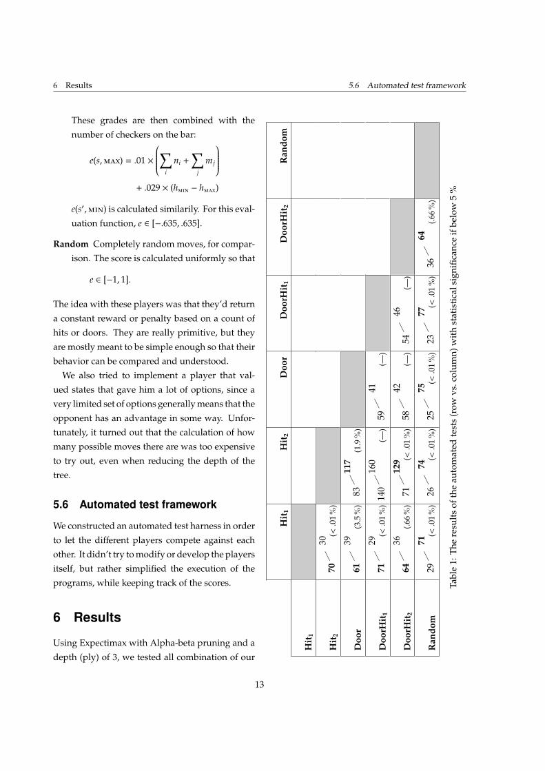
6 Results
Using Expectimax with Alpha-beta pruning and a
depth (ply) of 3, we tested all combination of our
Hit
1H
it2
Doo
rD
oorH
it1
Doo
rHit
2R
ando
m
Hit
1
Hit
270
30�
(<.0
1%
)
Doo
r61
39�
(3.5
%)
8311
7�
(1.9
%)
Doo
rHit
171
29�
(<.0
1%
)14
016
0�
(—)
5941
�(—
)
Doo
rHit
264
36�
(.66
%)
7112
9�
(<.0
1%
)58
42�
(—)
5446
�(—
)
Ran
dom
2971
�(<.0
1%
)26
74�
(<.0
1%
)25
75�
(<.0
1%
)23
77�
(<.0
1%
)36
64�
(.66
%)
Tabl
e1:
The
resu
lts
ofth
eau
tom
ated
test
s(r
owvs
.col
umn)
wit
hst
atis
tica
lsig
nific
ance
ifbe
low
5%
13

8 Further research
six players against each other. These tests were
generally performed in series of 100 games, but we
ran more games with a few of them, to get more
reliable results. The outcome of these tests can be
viewed in Table 1. For each result, we ran a two-
tailed sign test. We decided on a cut-off for our
presentation of p-values at 5 %. Anything above
that should be run a substantial number of times
more if we want to reach any conclusions.
First, we noted that the player Random loses to
all other players. This means that our AI play-
ers are working, as they are at least doing a better
job than pure randomness does. While we have
to admit that it was a bit discouraging that they
didn’t perform even better, we have to keep in
mind that they all use extremely basic strategies.
Even though there might be theoretical discussions
about the usage for a randomizing player, we had
no longer any need for it for the purpose of devel-
oping an evaluation function, and could therefore
discard it.
Having removed Random, we could clearly see
that Hit1 was losing to all the remaining play-
ers. Among the rest, however, the patterns are not
completely obvious. Of course, Hit2 performed
well against Door as well as against DoorHit2, but
DoorHit1 put up a good fight. Actually, when just
looking at the numbers, it seems like a cycle is al-
most formed as Hit2 is better than DoorHit2, which
is slightly better than DoorHit1, which is virtually
as good as Hit2. This reminds us of games like
rock-paper-scissors, where there is no absolute win-
ner but rather different ways of beating different
opponents. In our case, though, we concluded
that Hit2 outperformed all other players except for
one, which it still performed well against. Thus,
we declared Hit2 the winner.
7 Conclusions
The tests took a long time to run, and if we had
had the computational power to run more of them
we could’ve received results that were statistically
better. However, we believe that it wouldn’t have
changed anything.
Hit2 was the player that tried to hit the oppo-
nent’s blots while protecting its own. We find it
facinating that such a simple set of rules can prove
to be the dominant one, but are at the same time
surprised that the very similar Hit1 performed so
poorly. It seems that halfway right can be com-
pletely wrong. But the explanation for the success
of Hit2 might be that it turned out to be a good
strategy for building doors as well (since it dislikes
lonely checkers), while the purely door-building
player might not have been able to pose a threat to
the opponent, or even maintain an offensive posi-
tion on its own in the long run if it at the same time
wanted to maximize the number of doors.
We have managed to construct a player that out-
performs several other players, and especially a
random player. We do realize, however, that a hu-
man player would likely easily defeat it. The pro-
gram might perhaps be able to play against novice
human players, but it’s not difficult to understand
why modern backgammon programs are based on
artificial neural networks.
8 Further research
A possible continuation of this work, might be to
develop the test framework into one that auto-
matically runs tests for a long time while genet-
ically mutating different variables, and maybe also
using different evaluation functions with variable
weights. At the same time, tests against a human
14

References References
player would be interesting, to see to which level
this program could evolve.
Another interesting topic is whether similar stra-
tegies would work for the other games, explained
in section 3, if the players are used together with
different rule engines. What are the common de-
nominators for these games?
9 Acknowledgements
We’d like to thank Andreas Giallourakis for spend-
ing time teaching us the game.
References
[1] Backgammon Galore, http://www.bkgm.com/
[viewed 2011-04-14]
[2] Hauk, T., Buro, M. & Schaeffer, J. 2004, ’*-
Minimax Performance in Backgammon’, Pro-
ceedings of Computers and Games, pp. 51–
66, available online: http://skatgame.net/
mburo/ps/STAR-B.pdf [viewed 2011-04-14]
[3] Kalai, G. 2011, Is Backgammon in P?, blog en-
try, http://gilkalai.wordpress.com/2011/
01/14/is-backgammon-in-p/
[4] Nilsson, N. 1998, Artificial Intelligence: A New
Synthesis, Morgan Kaufmann, San Francisco,
USA
[5] Scott, J. 2001 The Neural Net Backgammon Pro-
grams, available online: http://satirist.
org/learn-game/systems/gammon/ [viewed
2011-04-14]
[6] Smed, J. & Hakonen, H. 2006, Algorithms and
Networks for Computer Games, John Wiley &
Sons, Ltd, West Sussex, England
[7] Tesauro, G. 1995, ’Temporal Difference Learn-
ing and TD-Gammon’, Communications of the
ACM, vol. 38, no. 3, March 1995, avail-
able online: http://www.research.ibm.com/
massive/tdl.html [viewed 2011-04-14]
[8] Veness, J. 2006, Expectimax Enhancements for
Stochastic Game Players, Bachelor thesis, The
University of New South Wales School of Com-
puter Science and Engineering, available on-
line: http://jveness.info/publications/
thesis.pdf [viewed 2011-04-14]
15

www.kth.se
Top Related